case-cohort design and secondary analysis - … design and secondary analysis ... cohort studies for...

Case-Cohort Design and Secondary Analysis

Yujie Zhong and Richard J. Cook

Department of Statistics and Actuarial Science, University of Waterloo

Yujie Zhong and Richard J. Cook Case-Cohort Design and Secondary Analysis

1 Introduction

2 Evolution of Research on The Case-Cohort Design

3 Secondary Analysis

4 Concluding Remarks


Introduction


Why?

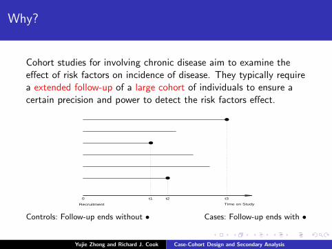
Cohort studies for involving chronic disease aim to examine theeffect of risk factors on incidence of disease. They typically requirea extended follow-up of a large cohort of individuals to ensure acertain precision and power to detect the risk factors effect.

●

●

●

Time on Study

t1 t2 t30

Recruitment

Controls: Follow-up ends without • Cases: Follow-up ends with •


Why?

The standard cohort design is

Expensive: Requires assembly of all covariate (exposure)histories

Inefficient: Measuring exposure in many controls is wasteful

Time-consuming: Requires extended follow-up to observe thedevelopment of the condition of interest


Why?

Example

Multiple risk factor intervention trial [1]

This trial is to determine whether a special intervention programwould result in a significant reduction in mortality from coronaryheart disease.

randomized 12,866 subjects, and followed up for seven years

cost more than $100 million

only 2% of MRFIT men experienced the primary endpoint ofcoronary heart disease mortality.

Alternative more cost-effective designs are needed:

Nested case-control design (Thomas, 1976)

Case-cohort design (Prentice, 1986)

∗ MRFIT Research Group (1982)


Nested Case-Control Design

In a nested case-control design, a number of “controls” from thoseat risk at the failure time of each case is selected.

∗Cases: • Controls: ◦∗ Samuelsen(2005)


Case Cohort Design

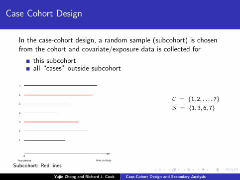
In the case-cohort design, a random sample (subcohort) is chosenfrom the cohort and covariate/exposure data is collected for

this subcohortall “cases” outside subcohort

Time on Study

0

1

2

3

4

5

6

7

Recruitment

Subcohort: Red lines

C = {1, 2, . . . , 7}S = {1, 3, 6, 7}


Case Cohort Design

In the case-cohort design, a random sample (subcohort) is chosenfrom the cohort and covariate/exposure data is collected for

this subcohortall “cases” outside subcohort

●

●

●

t1 t2 t3

Time on Study

0

1

2

3

4

5

6

7

Recruitment

Subcohort: Red lines Cases: •

C = {1, 2, . . . , 7}S = {1, 3, 6, 7}S∪D = {1, 3, 4, 6, 7}


Advantages of Case Cohort Design

Much lower total cost for measurement of exposure

More efficient than analysis based on subcohort only

Data from the subcohort selected in advance of follow-up canbe useful to study time varying markers

Enables analysis for a range of disease endpoints. . .


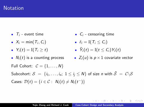
Notation

• Ti - event time • Ci - censoring time

• Xi = min(Ti ,Ci ) • δi = I(Ti ≤ Ci )

• Yi (t) = I(Ti ≥ t) • Yi (t) = I(t ≤ Ci )Yi (t)

• Ni (t) is a counting process • Zi (u) is p× 1 covariate vector

Full Cohort: C = {1, . . . ,N}

Subcohort: S = {i1, . . . , in; 1 ≤ ij ≤ N} of size n with S = C\S

Cases: D(t) = {i ∈ C : Ni (t) 6= Ni (t−)}


Recall: Estimation via Partial likelihood (Cox, 1972)

Under the Cox model

λ(t;Z (u), 0 ≤ u ≤ t) = λ0(t) exp(Z′(t)β)

The partial likelihood and score equation are

L(β) ∝N∏i=1

Yi (ti ) exp(Z′

i (ti )β)∑j∈C

Yj(ti ) exp(Z′j (ti )β)

δi

U(β) =N∑i=1

∞∫0

Yi (s)

Zi (s)−

∑j∈C

Yj(s) exp(Z′

j (s)β)Zj(s)∑j∈C

Yj(s) exp(Z′j (s)β)

dNi (s)


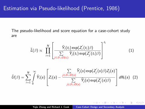
Estimation via Pseudo-likelihood (Prentice, 1986)

The pseudo-likelihood and score equation for a case-cohort studyare

L(β) ∝N∏i=1

Yi (ti ) exp(Z′

i (ti )β)∑j∈S∪D(ti )


δi

(1)

U(β) =N∑i=1

∞∫0

Yi (s)

Zi (s)−

∑j∈S∪D(s)

Yj(s) exp(Z′

j (s)β)Zj(s)∑j∈S∪D(s)

Yj(s) exp(Z′j (s)β)

dNi (s) (2)


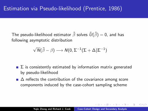
Estimation via Pseudo-likelihood (Prentice, 1986)

The pseudo-likelihood estimator β solves U(β) = 0, and hasfollowing asymptotic distribution

√N(β − β) −→ N(0,Σ−1(Σ + ∆)Σ−1)

Σ is consistently estimated by information matrix generatedby pseudo-likelihood

∆ reflects the contribution of the covariance among scorecomponents induced by the case-cohort sampling scheme


Evolution of Research on The Case-Cohort Design


Recent Methodologic Advances

Various estimating functions have been proposed to givedifferent estimators

Approaches to variance estimation have been explored

Alternative sampling schemes


A Comparison of Different Estimation Methods



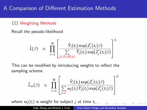
[I] Weighting Methods

Recall the pseudo-likelihood

L(β) ∝N∏i=1

Yi (ti ) exp(Z′i (ti )β)∑

j∈S∪D(ti )


δi

This can be modified by introducing weights to reflect thesampling scheme

Lw (β) ∝N∏i=1

Yi (ti ) exp(Z′i (ti )β)∑

j∈Cwj(ti )Yj(ti ) exp(Z

′j (ti )β)

δi

where wj(ti ) is weight for subject j at time ti .



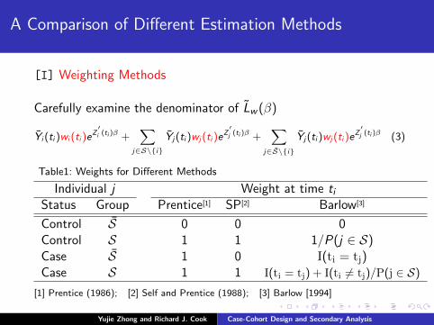
[I] Weighting Methods

Carefully examine the denominator of Lw (β)

Yi (ti )wi (ti )eZ′i (ti )β +

∑j∈S\{i}

Yj(ti )wj(ti )eZ′j (ti )β +

∑j∈S\{i}

Yj(ti )wj(ti )eZ′j (ti )β (3)

Table1: Weights for Different Methods

Individual j Weight at time tiStatus Group Prentice[1] SP[2] Barlow[3]

Control S 0 0 0Control S 1 1 1/P(j ∈ S)Case S 1 0 I(ti = tj)Case S 1 1 I(ti = tj) + I(ti 6= tj)/P(j ∈ S)

[1] Prentice (1986); [2] Self and Prentice (1988); [3] Barlow [1994]


Unbiasness of Weighted Score Equations

• Rj(t) = I(subject j contributes at t)

• πj(t) = Yj(t)dNj(t) + Yj(t)(1− dNj(t))P(j ∈ S|Yj(t) = 1,Zj(t))

• wj(t) = Rj(t)/πj(t)

Then score equations for case-cohort design are

U1(dΛ0(t), β) =N∑j=1

[Rj(t)

πj(t)

]{Yj(t) [dNj(t)− dΛj(t|Zj(t))]

}(4)

U2(dΛ0(t), β) =N∑j=1

∞∫0

[Rj(s)

πj(s)

]{Yj(s)Zj(s)

[dNj(s)− dΛ0(s)eZ

′j (s)β

]}(5)



Conditional expectation of Rj(s) given {Yj(s) = 1, dNj(s),Zj(s)},

E [Rj(s)|Yj(s) = 1, dNj(s),Zj(s)]

= Yj(s)(1− dNj(s))P(Rj(s) = 1|Yj(s) = 1, dNj(s) = 0,Zj(s))

+Yj(s)dNj(s)P(Rj(s) = 1|Yj(s) = 1, dNj(s) = 1,Zj(s))

= Yj(s)(1− dNj(s))P(j ∈ S|Yj(s) = 1, dNj(s) = 0,Zj(s))

+Yj(s)dNj(s)

= πj(s)



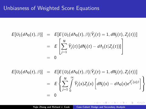
E [U1(dΛ0(t), β)] = E [E{U1(dΛ0(t), β)|Yj(t) = 1, dNj(t),Zj(t)}]

= E

N∑j=1

Yj(t) [dNj(t)− dΛj(t|Zj(t))]

= 0

E [U2(dΛ0(t), β)] = E [E{U2(dΛ0(t), β)|Yj(t) = 1, dNj(t),Zj(t)}]

= E

N∑j=1

∞∫0

Yj(s)Zj(s)

[dNj(s)− dΛ0(s)eZ

′j (s)β

]= 0


Estimation Methods

[II] Weighted Estimating Equations: Chen and Lo (1999)suggested a class of estimating functions that in many casesimproved efficiency.

[III] Cohort study for missing data: Lin and Ying (1993)proposed an approximate partial likelihood method for missingcovariate problem under Cox model, and applied that in acase-cohort study.


Variance Estimation


Variance Estimation

Self and Prentice (1988)

Derive the asymptotic variance

Wacholder et al (1989)

Bootstrap variance estimation

Barlow (1994)

Robust variance estimation


Sampling Schemes


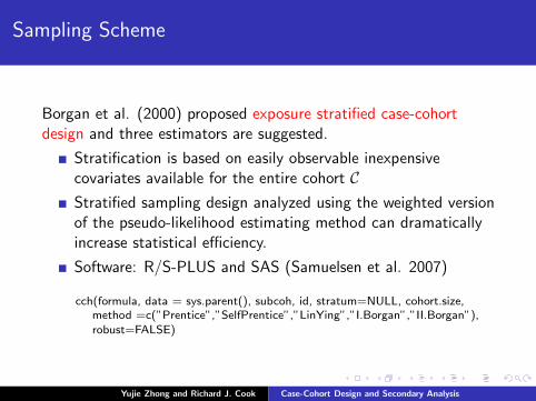
Sampling Scheme

Borgan et al. (2000) proposed exposure stratified case-cohortdesign and three estimators are suggested.

Stratification is based on easily observable inexpensivecovariates available for the entire cohort CStratified sampling design analyzed using the weighted versionof the pseudo-likelihood estimating method can dramaticallyincrease statistical efficiency.

Software: R/S-PLUS and SAS (Samuelsen et al. 2007)

cch(formula, data = sys.parent(), subcoh, id, stratum=NULL, cohort.size,method =c(”Prentice”,”SelfPrentice”,”LinYing”,”I.Borgan”,”II.Borgan”),robust=FALSE)


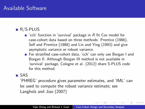
Available Software

R/S-PLUS

’cch’ function in ’survival’ package in R fit Cox model forcase-cohort data based on three methods: Prentice (1986),Self and Prentice (1988) and Lin and Ying (1993) and giveasymptotic variance or robust variance.For stratified case-cohort data, ’cch’ can only use Borgan I andBorgan II. Although Borgan III method is not available in’survival’ package, Cologne et al. (2012) share S-PLUS codefor this method.

SAS’PHREG’ procedure gives parameter estimates, and ’IML’ canbe used to compute the robust variance estimate; seeLangholz and Jiao (2007)


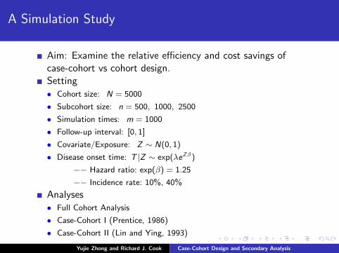
A Simulation Study

Aim: Examine the relative efficiency and cost savings ofcase-cohort vs cohort design.Setting• Cohort size: N = 5000

• Subcohort size: n = 500, 1000, 2500

• Simulation times: m = 1000

• Follow-up interval: [0, 1]

• Covariate/Exposure: Z ∼ N(0, 1)

• Disease onset time: T |Z ∼ exp(λeZβ)

−− Hazard ratio: exp(β) = 1.25

−− Incidence rate: 10%, 40%

Analyses• Full Cohort Analysis

• Case-Cohort I (Prentice, 1986)

• Case-Cohort II (Lin and Ying, 1993)


A Simulation Study

Table 2: Estimation results (10% Disease Incidence, N = 5000)

n=500 n=1000 n=2500Method BIAS ASE ESE BIAS ASE ESE BIAS ASE ESECohort 1e-05 .044 .045 .002 .044 .046 .003 .044 .044CCP .002 .069 .062 .003 .057 .056 .003 .047 .047CCLY .002 .063 .062 .003 .053 .055 .003 .047 .046

Table 3: Estimation results (40% Disease Incidence, N = 5000)

n=500 n=1000 n=2500Method BIAS ASE ESE BIAS ASE ESE BIAS ASE ESECohort -15e-04 .023 .024 -4e-05 .023 .023 4e-05 .022 .023CCP -6e-04 .021 .054 3e-04 .043 .040 -1e-04 .029 .028CCLY -9e-04 .048 .050 -3e-04 .036 .037 -4e-05 .027 .027


A Simulation Study: Consider Cost Saving

1000 2000 3000 4000 5000

050

100

150

TOTOAL COST

FR

EQ

UE

NC

Y

n = 500

1000 2000 3000 4000 5000

050

100

150

200

250

TOTOAL COST

FR

EQ

UE

NC

Y

n = 2500

1000 2000 3000 4000 5000

050

100

150

200

TOTOAL COST

FR

EQ

UE

NC

Y

n = 500

1000 2000 3000 4000 5000

050

100

150

200

250

300

TOTOAL COST

FR

EQ

UE

NC

Y

n = 2500

Fig1: Histogram for cost for case-cohort design (upper: 10%, bottom: 40%)


Multiple Disease Outcomes

Able to study multiple outcomes individually without having toobtain separate sets of comparison subjects.However, this aspect is seldom illustrated or examined in literature.

Sφrensen and Andersen (2000)

investigate competing risk of multiple outcomes forcase-cohort designwhen all case groups are compared with the same sub-cohort,a correlation is induced between estimated exposures effects ondifferent outcomes.Correlations increase with smaller subcohort sampling fractions.

Kang and Cai (2009)

Simultaneously model the times to different events to comparethe effect of a risk factor on different types of diseasesMarginal proportional hazards regression models are proposedfor case-cohort studies with multiple disease outcomes.


Secondary Analysis


Secondary Analysis

Uses existing data to investigate research questions other thanthe main ones for which the data were originally gathered(Hulley et al., 2007)

Can supplement the primary analysis and guide scientificinquiry, or it might be the primary interest for subsequentresearch

There has been little discussion of statistical issues arising insecondary analysis of case-cohort data


Secondary Analysis for Case-Control Design

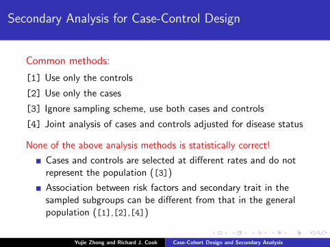
Common methods:

[1] Use only the controls

[2] Use only the cases

[3] Ignore sampling scheme, use both cases and controls

[4] Joint analysis of cases and controls adjusted for disease status

None of the above analysis methods is statistically correct!

Cases and controls are selected at different rates and do notrepresent the population ([3])

Association between risk factors and secondary trait in thesampled subgroups can be different from that in the generalpopulation ([1],[2],[4])


Secondary Analysis for Case-Control Design

Lin and Zeng (2009)

Proposed a new likelihood based method that reflects thecase-control sampling (retrospective form and based ondisease status)

After specifying P(Yi |Xi ) (linear or logistic regression) andP(Di = 1|Xi ,Yi ) (logistic regression), the likelihood is

L =n∏

i=1

P(Yi ,Xi |Di )

where Yi is secondary trait, Di is case-control status, and Xi

are covariate.

∗ Lee, McMurchy and Scott (1997); Jiang, Scott and Wild (2006)


Secondary Analysis For Case-Cohort Design


Copula Function

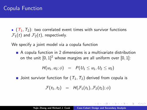
• (T1,T2): two correlated event times with survivor functionsF1(t) and F2(t), respectively.

We specify a joint model via a copula function

A copula function in 2 dimensions is a multivariate distributionon the unit [0, 1]2 whose margins are all uniform over [0, 1]:

H(u1, u2;φ) = P(U1 ≤ u1,U2 ≤ u2)

Joint survivor function for (T1,T2) derived from copula is

F(t1, t2) = H(F1(t1),F2(t2);φ)


Secondary Analysis for Case-cohort Design

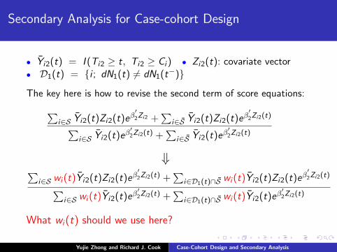
• Yi2(t) = I (Ti2 ≥ t, Ti2 ≥ Ci ) • Zi2(t): covariate vector• D1(t) = {i ; dN1(t) 6= dN1(t−)}

The key here is how to revise the second term of score equations:∑i∈S Yi2(t)Zi2(t)eβ

′2Zi2 +

∑i∈S Yi2(t)Zi2(t)eβ

′2Zi2(t)∑

i∈S Yi2(t)eβ′2Zi2(t) +

∑i∈S Yi2(t)eβ

′2Zi2(t)

⇓∑i∈S wi (t)Yi2(t)Zi2(t)eβ

′2Zi2(t) +

∑i∈D1(t)∩S wi (t)Yi2(t)Zi2(t)eβ

′2Zi2(t)∑

i∈S wi (t)Yi2(t)eβ′2Zi2(t) +

∑i∈D1(t)∩S wi (t)Yi2(t)eβ

′2Zi2(t)

What wi(t) should we use here?


Secondary Analysis for Case-Cohort Design

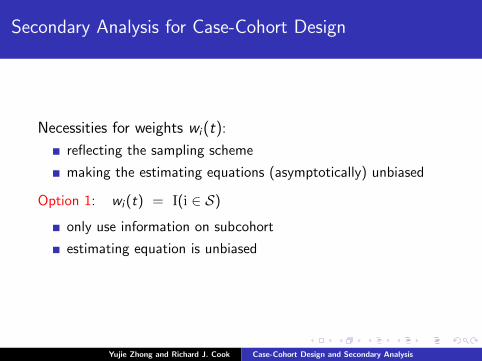
Necessities for weights wi(t):

reflecting the sampling scheme

making the estimating equations (asymptotically) unbiased

Option 1: wi (t) = I(i ∈ S)

only use information on subcohort

estimating equation is unbiased



Our aim: make use of available information outside the subcohort.

For i ∈ S, wi (t) can be the same as before, i.e. 1 or inverseprobability weights

The key question is how to choose wi (t) for i ∈ D1(t) ∩ S∗Option 2:

wi (t) = I(Ti1 ≤ Ci )/P(Ti1 ≤ Ci |Ti2 ≥ t), for i ∈ D1(t) ∩ S

This can be estimated parametrically or nonparametrically.



Next Step:

Prove the (asymptotic) unbiasness of the implied estimatingequation

Find the asymptotic distribution of estimator

Find the estimates of parameters and asymptotic variance

Simulation and application


Summary & Comments

Case-cohort designs offer a cost-effective method ofestimating the effects of risk factors in setting with lowdisease incidence and covariates which are costly to measure

Since all cases are used there is little loss in precision or power

Potential use in genomic and other biomarker studies isconsiderable

A variety of weighting schemes can be explored to extract asmuch information from data as possible

Methods for conducting valid secondary analyses are on going


case-cohort design and secondary analysis - … design and secondary analysis ... cohort studies for...

Documents