case study: applying generalized - mit opencourseware · 2020-01-03 · mccullagh and nelder (1989)...
TRANSCRIPT
Case Study Applying Generalized Linear Models
Dr Kempthorne
May 12 2016
Contents
1 Generalized Linear Models of Semi-Quantal Biological Assay Data 2 11 Coal miners Pneumoconiosis Data 2 12 Multinomial Model for Incidence Counts 4 13 Proportional Odds Model Parallel Linear Logit Model 11 14 GeneralIndependent Linear Logit Models 14 15 Likelihood-Ratio Test of Proportional Odds 16 16 References 17
1
1 Generalized Linear Models of Semi-Quantal Biological Assay Data
11 Coal miners Pneumoconiosis Data
McCullagh and Nelder (1989) discuss the application of generalized linear modshyels to modeling the incidence and severity of lung disease in coal miners as it relates to the degree of exposure to coal dust They introduce the data as follows
The data taken from Ashford (1959) concern the degree of pneumoshyconiosis in coalface workers as a function of exposure t measured in years Severity of disease is measured radiologically and is of necesshysity qualitative A four-category version of the ILO rating scale was used initially but the two most severe categories were subsequently combined
McCullagh and Nelder (1989) p 179
Using R and Yeersquos (2010) R-package VGAM (Vector Generalized Linear and Additive Models) we load in the data set pneumo compute summary statistics and plots
gt 01 Load R packages ==== gt require(stats) gt require(graphics) gt library(VGAM) gt 11 Display and summarize dataset pneumo ==== gt print(pneumo)
exposuretime normal mild severe 1 58 98 0 0 2 150 51 2 1 3 215 34 6 3 4 275 35 5 8 5 335 32 10 9 6 395 23 7 8 7 460 12 6 10 8 515 4 2 5
gt summary(pneumo)
exposuretime normal mild severe Min 580 Min 400 Min 000 Min 000 1st Qu1988 1st Qu2025 1st Qu 200 1st Qu 250 Median 3050 Median 3300 Median 550 Median 650 Mean 3004 Mean 3612 Mean 475 Mean 550 3rd Qu4112 3rd Qu3900 3rd Qu 625 3rd Qu 825 Max 5150 Max 9800 Max 1000 Max 1000
2
gt
gt 12 Plot data gt gt Attaching the dataset allows access to column variables using their names gt gt names(pneumo)
[1] exposuretime normal mild severe
gt attach(pneumo) gt matrixcountslt-t(asmatrix(pneumo[24])) gt dimnames(matrixcounts)[[2]]lt-paste( ascharacter(pneumo$exposuretime) Yrssep=) gt barplot(matrixcounts beside=TRUE col=(c(123)) + legendtext=(c(normalmildsevere)) + cexnames=5 + ylab=Countsmain=Pneumoconiosis Data Category Counts by Exposure Time + xlab=Exposure Time) gt
58 Yrs 15 Yrs 215 Yrs 275 Yrs 335 Yrs 395 Yrs 46 Yrs 515 Yrs
normalmildsevere
Pneumoconiosis Data Category Counts by Exposure Time
Exposure Time
Cou
nts
020
4060
80
3
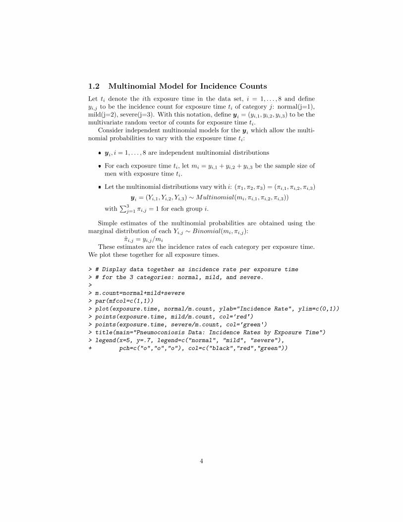
12 Multinomial Model for Incidence Counts
Let ti denote the ith exposure time in the data set i = 1 8 and define yij to be the incidence count for exposure time ti of category j normal(j=1) mild(j=2) severe(j=3) With this notation define yi = (yi1 yi2 yi3) to be the multivariate random vector of counts for exposure time ti
Consider independent multinomial models for the yi which allow the multishynomial probabilities to vary with the exposure time ti
bull yi i = 1 8 are independent multinomial distributions
bull For each exposure time ti let mi = yi1 + yi2 + yi3 be the sample size of men with exposure time ti
bull Let the multinomial distributions vary with i (π1 π2 π3) = (πi1 πi2 πi3)
yi = (Yi1 Yi2 Yi3) sim Multinomial(mi πi1 πi2 πi3)) 3with πij = 1 for each group ij=1
Simple estimates of the multinomial probabilities are obtained using the marginal distribution of each Yij sim Binomial(mi πij )
πij = yij mi
These estimates are the incidence rates of each category per exposure time We plot these together for all exposure times
gt Display data together as incidence rate per exposure time gt for the 3 categories normal mild and severe gt gt mcount=normal+mild+severe gt par(mfcol=c(11)) gt plot(exposuretime normalmcount ylab=Incidence Rate ylim=c(01)) gt points(exposuretime mildmcount col=red) gt points(exposuretime severemcount col=green) gt title(main=Pneumoconiosis Data Incidence Rates by Exposure Time) gt legend(x=5 y=7 legend=c(normal mild severe) + pch=c(ooo) col=c(blackredgreen))
4
10 20 30 40 50
00
02
04
06
08
10
exposuretime
Inci
denc
e R
ate
Pneumoconiosis Data Incidence Rates by Exposure Time
ooo
normalmildsevere
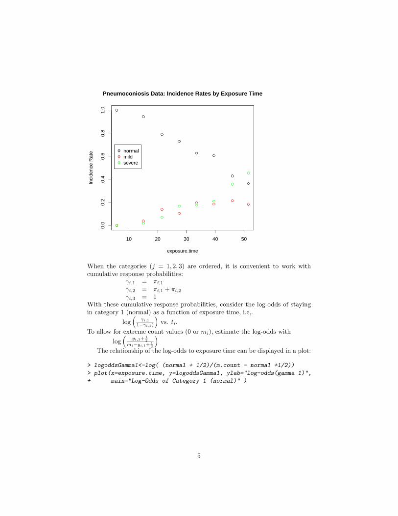
When the categories (j = 1 2 3) are ordered it is convenient to work with cumulative response probabilities
γi1 = πi1
γi2 = πi1 + πi2
γi3 = 1 With these cumulative response probabilities consider the log-odds of staying in category 1 (normal) as a function of exposure time ie o u
γi1log vs ti1minusγi1)
To allow for extreme count values (0 or mi) estimate the log-odds with o 1 u
yi1+ 2log 1 miminusyi1+ 2
The relationship of the log-odds to exposure time can be displayed in a plot
gt logoddsGamma1lt-log( (normal + 12)(mcount - normal +12)) gt plot(x=exposuretime y=logoddsGamma1 ylab=log-odds(gamma 1) + main=Log-Odds of Category 1 (normal) )
5
10 20 30 40 50
01
23
45
LogminusOdds of Category 1 (normal)
exposuretime
logminus
odds
(gam
ma
1)
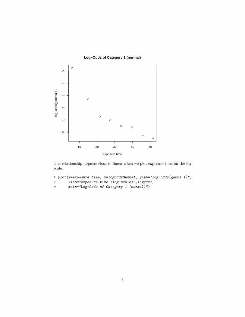
The relationship appears close to linear when we plot exposure time on the log scale
gt plot(x=exposuretime y=logoddsGamma1 ylab=log-odds(gamma 1) + xlab=exposuretime (log-scale)log=x + main=Log-Odds of Category 1 (normal))
6
10 20 50
01
23
45
LogminusOdds of Category 1 (normal)
exposuretime (logminusscale)
logminus
odds
(gam
ma
1)
Analogous computations and plots are made for the log-odds of the pooled rdquonon-severerdquo category (normal plus mild) Using the following estimate for the log-odds we plot the relationship o u
1 yi1+yi2+ 2with log 1 miminusyi1 minusyi2+ 2
gt logoddsGamma2lt-log( (normal + mild +12)(mcount - normal -mild +12)) gt plot(x=exposuretime y=logoddsGamma2 ylab=log-odds(gamma 2)col=2 + main=Log-Odds of Pooled Categoryn(non-severe = normal + mild))
7
10 20 30 40 50
01
23
45
LogminusOdds of Pooled Category(nonminussevere = normal + mild)
exposuretime
logminus
odds
(gam
ma
2)
Again the relationship appears close to linear when we plot exposure time on the log scale
gt plot(x=exposuretime y=logoddsGamma2 ylab=log-odds(gamma 2) + xlab=exposuretime (log-scale) log=xcol=2 + main=Log-Odds of Pooled Categoryn(non-severe = normal + mild))
8
10 20 50
01
23
45
LogminusOdds of Pooled Category(nonminussevere = normal + mild)
exposuretime (logminusscale)
logminus
odds
(gam
ma
2)
To compare these log-odds relationships with exposure time we plot them together
gt plot(x=exposuretime y=logoddsGamma1 ylab=log-odds + xlab=exposuretime (log-scale)log=x + main=Log-Odds type=b) gt lines(x=exposuretime y=logoddsGamma2 + type=bcol=red) gt legend(x=6y=2 + legend=c(normal Category non-severe Category (normal+mild)) + col=c(blackred) lty=c(11)cex=6)
9
10 20 50
01
23
45
LogminusOdds
exposuretime (logminusscale)
logminus
odds
normal Categorynonminussevere Category (normal+mild)
10
---
13 Proportional Odds Model Parallel Linear Logit Model
McCullagh and Nelder comment that these plots of the transformed variables suggest considering the model
log[γij (1 minus γij )] = θj minus β log ti j = 1 2 i = 1 8 Yeersquos (2010) R-package VGAM (Vector Generalized Linear and Additive Modshyels) provides the function vglm() to fit this model
gt pneumo lt- transform(pneumo logexpostime = log(exposuretime)) gt fit1lt-vglm(cbind(normal mild severe) ~ logexpostime + cumulative(reverse=FALSE parallel=TRUE)data = pneumo)
The R object fit1 (a class vglm object) provides details of the fitted genershyalized linear model First print a summary of the fit
gt summary(fit1)
Call vglm(formula = cbind(normal mild severe) ~ logexpostime
family = cumulative(reverse = FALSE parallel = TRUE) data = pneumo)
Pearson residuals Min 1Q Median 3Q Max
logit(P[Ylt=1]) -1248 -007164 01441 03086 07714 logit(P[Ylt=2]) -1044 -018415 03093 03353 05048
Coefficients Estimate Std Error z value Pr(gt|z|)
(Intercept)1 96761 13241 7308 272e-13 (Intercept)2 105817 13454 7865 369e-15 logexpostime -25968 03811 -6814 950e-12
Signif codes 0 0001 001 005 01 1
Number of linear predictors 2
Names of linear predictors logit(P[Ylt=1]) logit(P[Ylt=2])
Dispersion Parameter for cumulative family 1
Residual deviance 50268 on 13 degrees of freedom
Log-likelihood -250903 on 13 degrees of freedom
Number of iterations 4
Exponentiated coefficients
11
logexpostime 007451115
Important components of the summary are
bull Coefficients maximum-likelihood estimates of the model parameters In addition to the Estimates estimates of their standard deviation (Std Error) their ratio (z value) and the P-value for the (asymptotic) test of whether the underlying coefficient is zero
Note the coefficients specify the parallel lines defining the log-odds as a function of the log(exposure time)
bull Log-Likelihood minus250903 on 13 degrees of freedom
Note the degrees of freedom are the total degrees of freedom (8 times (3 minus 1)) minus the number of estimated parameters 3
bull Residual deviance (see Deviance definition in lecture notes)
To the plot of observed log-odds vs exposure-time we add the ML-Fitted log-odds according to the (parallel) cumulative log-odds model
gt plot(x=exposuretime y=logoddsGamma1 ylab=log-odds + xlab=exposuretime (log-scale)log=x + main=Log-Odds Observed and Parallel Fits type=bylim=c(min(logoddsGamma1) 6)) gt lines(x=exposuretime y=logoddsGamma2 + type=bcol=red) gt lines(exposuretime y=fit1predictors[1]type=blty=2 col=black) gt lines(exposuretime y=fit1predictors[2]type=blty=2 col=red) gt legend(x=6y=2 + legend=c(normal Category non-severe Category (normal+mild) + Fitted normal Category Fitted non-severe Category (normal+mild)) + col=c(blackredblackred) lty=c(1122)cex=6)
12
10 20 50
01
23
45
6
LogminusOdds Observed and Parallel Fits
exposuretime (logminusscale)
logminus
odds
normal Categorynonminussevere Category (normal+mild)Fitted normal CategoryFitted nonminussevere Category (normal+mild)
The vglm object fit1 includes fitted values for the multinomial probabilities These are printed out together with the observed frequencies
gt pneumorateslt-dataframe(exposuretime normal= normalmcount + mild=mildmcount severe=severemcount) gt pneumofittedrateslt-dataframe(cbind(exposuretimefit1fittedvalues)) gt print(cbind(pneumorates pneumofittedrates)digits=3)
exposuretime normal mild severe exposuretime normal mild severe 1 58 1000 0000 00000 58 0994 000356 000243 2 150 0944 0037 00185 150 0934 003843 002794 3 215 0791 0140 00698 215 0847 008509 006821 4 275 0729 0104 01667 275 0745 013364 012181 5 335 0627 0196 01765 335 0636 017615 018802 6 395 0605 0184 02105 395 0532 020558 026210 7 460 0429 0214 03571 460 0434 022078 034536 8 515 0364 0182 04545 515 0364 022202 041430
13
---
14 GeneralIndependent Linear Logit Models
The model of the previous section assumes parallel linear log-odds relationships on log exposure time A more general model allows these lines to have different slopes
The R-code below fits this model
gt pneumo lt- transform(pneumo logexpostime = log(exposuretime)) gt fit2lt-vglm(cbind(normal mild severe) ~ logexpostime + cumulative(reverse=FALSE parallel=FALSE)data = pneumo)
The R object fit2 (a class vglm object) provides details of the fitted genshyeralized linear model We print out the summary of this fit and focus on the coefficients corresponding to the slope parameters
gt summary(fit2)
Call vglm(formula = cbind(normal mild severe) ~ logexpostime
family = cumulative(reverse = FALSE parallel = FALSE) data = pneumo)
Pearson residuals Min 1Q Median 3Q Max
logit(P[Ylt=1]) -115 -01457 01249 03824 07288 logit(P[Ylt=2]) -115 -00506 01886 02864 05659
Coefficients Estimate Std Error z value Pr(gt|z|)
(Intercept)1 95933 13308 7208 566e-13 (Intercept)2 111048 18930 5866 445e-09 logexpostime1 -25713 03839 -6698 211e-11 logexpostime2 -27435 05323 -5155 254e-07
Signif codes 0 0001 001 005 01 1
Number of linear predictors 2
Names of linear predictors logit(P[Ylt=1]) logit(P[Ylt=2])
Dispersion Parameter for cumulative family 1
Residual deviance 48844 on 12 degrees of freedom
Log-likelihood -250191 on 12 degrees of freedom
Number of iterations 6
14
Exponentiated coefficients logexpostime1 logexpostime2
007643613 006434155
Important components of the summary are
bull Coefficients maximum-likelihood estimates of the model parameters In addition to the Estimates estimates of their standard deviation (Std Error) their ratio (z value) and the P-value for the (asymptotic) test of whether the underlying coefficient is zero
Note the coefficients specify two lines
logit(P [Y le 1]) = [(Intercept) 1]+[logexpostime 1]timeslog(ExposureT ime)
logit(P [Y le 2]) = [(Intercept) 2]+[logexpostime 2]timeslog(ExposureT ime)
The estimated slopes are very close minus25713 versus minus27435 and very similar to the slope of minus25968 in the first model
bull Log-Likelihood minus250191 on 12 degrees of freedom
Note the degrees of freedom are the total degrees of freedom (8 times (3 minus 1)) minus the number of estimated parameters 4 (two intercepts and two slopes)
The ML-Fitted log-odds according to this (non-parallel) cumulative log-odds model can be added to the plot given before
gt plot(x=exposuretime y=logoddsGamma1 ylab=log-odds + xlab=exposuretime (log-scale)log=x + main=Log-Odds Observed Parallel and Non-Parallel Fits + type=bylim=c(min(logoddsGamma1) 7)) gt lines(x=exposuretime y=logoddsGamma2 + type=bcol=red) gt lines(exposuretime y=fit1predictors[1]type=blty=2 col=black) gt lines(exposuretime y=fit1predictors[2]type=blty=2 col=red) gt lines(exposuretime y=fit2predictors[1]type=blty=2 col=bluelwd=2) gt lines(exposuretime y=fit2predictors[2]type=blty=2 col=greenlwd=2) gt legend(x=12y=7 + legend=c(normal Category non-severe Category (normal+mild) + Fit1 normal Category Fit1 non-severe Category (normal+mild) + Fit2 normal Category Fit2 non-severe Category (normal+mild)) + col=c(blackredblackredgreenblue) lty=c(112222) + lwd=c(111122)cex=8)
15
10 20 50
02
46
LogminusOdds Observed Parallel and NonminusParallel Fits
exposuretime (logminusscale)
logminus
odds
normal Categorynonminussevere Category (normal+mild)Fit1 normal CategoryFit1 nonminussevere Category (normal+mild)Fit2 normal CategoryFit2 nonminussevere Category (normal+mild)
This plot demonstrates that model fit2 with independent linear logit funcshytions is very close to model fit1 with parallel linear logit functions
15 Likelihood-Ratio Test of Proportional Odds
We use the V GAM -package function lrtest vglm to conduct a likelihood ratio test comparing the two models
gt lrtest_vglm(fit2fit1)
Likelihood ratio test
Model 1 cbind(normal mild severe) ~ logexpostime Model 2 cbind(normal mild severe) ~ logexpostime Df LogLik Df Chisq Pr(gtChisq)
1 12 -25019 2 13 -25090 1 01424 07059
gt
Note that the likelihood ratio test statistic is LR minus Statistic = minus2 times (Log minus likelihood[fit1] minus Log minus Likelihood[fit2])
= minus2 times (minus250903 minus [minus250191]) = minus2 times (+0712) = +1424
16
Under the null hypothesis of no improvement allowing the slopes of the log-odds functions to be different the statistic is asymptotically distributed as a Chi-Square random variable with degrees of freedom equal to the difference in degrees of freedom of the two models (1 in this case) The large P-Value (07059 gtgt 005) indicates that improvement of model fit2 over model fit1 is not statistically significant
16 References
Ashford (1959) An Approach to the analysis of data for semi-quantal responses in biological assay Biometrics 15 573-81
McCullagh and Nelder (1989) Generalized Linear Models 2nd Ed Chapman and Hall New York
Yee T W (2010) The VGAM package for categorical data analysis Journal of Statistical Software 32 1-34 httpwwwjstatsoftorgv32i10
17
MIT OpenCourseWarehttpocwmitedu
18655 Mathematical StatisticsSpring 2016
For information about citing these materials or our Terms of Use visit httpocwmiteduterms

1 Generalized Linear Models of Semi-Quantal Biological Assay Data
11 Coal miners Pneumoconiosis Data
McCullagh and Nelder (1989) discuss the application of generalized linear modshyels to modeling the incidence and severity of lung disease in coal miners as it relates to the degree of exposure to coal dust They introduce the data as follows
The data taken from Ashford (1959) concern the degree of pneumoshyconiosis in coalface workers as a function of exposure t measured in years Severity of disease is measured radiologically and is of necesshysity qualitative A four-category version of the ILO rating scale was used initially but the two most severe categories were subsequently combined
McCullagh and Nelder (1989) p 179
Using R and Yeersquos (2010) R-package VGAM (Vector Generalized Linear and Additive Models) we load in the data set pneumo compute summary statistics and plots
gt 01 Load R packages ==== gt require(stats) gt require(graphics) gt library(VGAM) gt 11 Display and summarize dataset pneumo ==== gt print(pneumo)
exposuretime normal mild severe 1 58 98 0 0 2 150 51 2 1 3 215 34 6 3 4 275 35 5 8 5 335 32 10 9 6 395 23 7 8 7 460 12 6 10 8 515 4 2 5
gt summary(pneumo)
exposuretime normal mild severe Min 580 Min 400 Min 000 Min 000 1st Qu1988 1st Qu2025 1st Qu 200 1st Qu 250 Median 3050 Median 3300 Median 550 Median 650 Mean 3004 Mean 3612 Mean 475 Mean 550 3rd Qu4112 3rd Qu3900 3rd Qu 625 3rd Qu 825 Max 5150 Max 9800 Max 1000 Max 1000
2
gt
gt 12 Plot data gt gt Attaching the dataset allows access to column variables using their names gt gt names(pneumo)
[1] exposuretime normal mild severe
gt attach(pneumo) gt matrixcountslt-t(asmatrix(pneumo[24])) gt dimnames(matrixcounts)[[2]]lt-paste( ascharacter(pneumo$exposuretime) Yrssep=) gt barplot(matrixcounts beside=TRUE col=(c(123)) + legendtext=(c(normalmildsevere)) + cexnames=5 + ylab=Countsmain=Pneumoconiosis Data Category Counts by Exposure Time + xlab=Exposure Time) gt
58 Yrs 15 Yrs 215 Yrs 275 Yrs 335 Yrs 395 Yrs 46 Yrs 515 Yrs
normalmildsevere
Pneumoconiosis Data Category Counts by Exposure Time
Exposure Time
Cou
nts
020
4060
80
3
12 Multinomial Model for Incidence Counts
Let ti denote the ith exposure time in the data set i = 1 8 and define yij to be the incidence count for exposure time ti of category j normal(j=1) mild(j=2) severe(j=3) With this notation define yi = (yi1 yi2 yi3) to be the multivariate random vector of counts for exposure time ti
Consider independent multinomial models for the yi which allow the multishynomial probabilities to vary with the exposure time ti
bull yi i = 1 8 are independent multinomial distributions
bull For each exposure time ti let mi = yi1 + yi2 + yi3 be the sample size of men with exposure time ti
bull Let the multinomial distributions vary with i (π1 π2 π3) = (πi1 πi2 πi3)
yi = (Yi1 Yi2 Yi3) sim Multinomial(mi πi1 πi2 πi3)) 3with πij = 1 for each group ij=1
Simple estimates of the multinomial probabilities are obtained using the marginal distribution of each Yij sim Binomial(mi πij )
πij = yij mi
These estimates are the incidence rates of each category per exposure time We plot these together for all exposure times
gt Display data together as incidence rate per exposure time gt for the 3 categories normal mild and severe gt gt mcount=normal+mild+severe gt par(mfcol=c(11)) gt plot(exposuretime normalmcount ylab=Incidence Rate ylim=c(01)) gt points(exposuretime mildmcount col=red) gt points(exposuretime severemcount col=green) gt title(main=Pneumoconiosis Data Incidence Rates by Exposure Time) gt legend(x=5 y=7 legend=c(normal mild severe) + pch=c(ooo) col=c(blackredgreen))
4
10 20 30 40 50
00
02
04
06
08
10
exposuretime
Inci
denc
e R
ate
Pneumoconiosis Data Incidence Rates by Exposure Time
ooo
normalmildsevere
When the categories (j = 1 2 3) are ordered it is convenient to work with cumulative response probabilities
γi1 = πi1
γi2 = πi1 + πi2
γi3 = 1 With these cumulative response probabilities consider the log-odds of staying in category 1 (normal) as a function of exposure time ie o u
γi1log vs ti1minusγi1)
To allow for extreme count values (0 or mi) estimate the log-odds with o 1 u
yi1+ 2log 1 miminusyi1+ 2
The relationship of the log-odds to exposure time can be displayed in a plot
gt logoddsGamma1lt-log( (normal + 12)(mcount - normal +12)) gt plot(x=exposuretime y=logoddsGamma1 ylab=log-odds(gamma 1) + main=Log-Odds of Category 1 (normal) )
5
10 20 30 40 50
01
23
45
LogminusOdds of Category 1 (normal)
exposuretime
logminus
odds
(gam
ma
1)
The relationship appears close to linear when we plot exposure time on the log scale
gt plot(x=exposuretime y=logoddsGamma1 ylab=log-odds(gamma 1) + xlab=exposuretime (log-scale)log=x + main=Log-Odds of Category 1 (normal))
6
10 20 50
01
23
45
LogminusOdds of Category 1 (normal)
exposuretime (logminusscale)
logminus
odds
(gam
ma
1)
Analogous computations and plots are made for the log-odds of the pooled rdquonon-severerdquo category (normal plus mild) Using the following estimate for the log-odds we plot the relationship o u
1 yi1+yi2+ 2with log 1 miminusyi1 minusyi2+ 2
gt logoddsGamma2lt-log( (normal + mild +12)(mcount - normal -mild +12)) gt plot(x=exposuretime y=logoddsGamma2 ylab=log-odds(gamma 2)col=2 + main=Log-Odds of Pooled Categoryn(non-severe = normal + mild))
7
10 20 30 40 50
01
23
45
LogminusOdds of Pooled Category(nonminussevere = normal + mild)
exposuretime
logminus
odds
(gam
ma
2)
Again the relationship appears close to linear when we plot exposure time on the log scale
gt plot(x=exposuretime y=logoddsGamma2 ylab=log-odds(gamma 2) + xlab=exposuretime (log-scale) log=xcol=2 + main=Log-Odds of Pooled Categoryn(non-severe = normal + mild))
8
10 20 50
01
23
45
LogminusOdds of Pooled Category(nonminussevere = normal + mild)
exposuretime (logminusscale)
logminus
odds
(gam
ma
2)
To compare these log-odds relationships with exposure time we plot them together
gt plot(x=exposuretime y=logoddsGamma1 ylab=log-odds + xlab=exposuretime (log-scale)log=x + main=Log-Odds type=b) gt lines(x=exposuretime y=logoddsGamma2 + type=bcol=red) gt legend(x=6y=2 + legend=c(normal Category non-severe Category (normal+mild)) + col=c(blackred) lty=c(11)cex=6)
9
10 20 50
01
23
45
LogminusOdds
exposuretime (logminusscale)
logminus
odds
normal Categorynonminussevere Category (normal+mild)
10
---
13 Proportional Odds Model Parallel Linear Logit Model
McCullagh and Nelder comment that these plots of the transformed variables suggest considering the model
log[γij (1 minus γij )] = θj minus β log ti j = 1 2 i = 1 8 Yeersquos (2010) R-package VGAM (Vector Generalized Linear and Additive Modshyels) provides the function vglm() to fit this model
gt pneumo lt- transform(pneumo logexpostime = log(exposuretime)) gt fit1lt-vglm(cbind(normal mild severe) ~ logexpostime + cumulative(reverse=FALSE parallel=TRUE)data = pneumo)
The R object fit1 (a class vglm object) provides details of the fitted genershyalized linear model First print a summary of the fit
gt summary(fit1)
Call vglm(formula = cbind(normal mild severe) ~ logexpostime
family = cumulative(reverse = FALSE parallel = TRUE) data = pneumo)
Pearson residuals Min 1Q Median 3Q Max
logit(P[Ylt=1]) -1248 -007164 01441 03086 07714 logit(P[Ylt=2]) -1044 -018415 03093 03353 05048
Coefficients Estimate Std Error z value Pr(gt|z|)
(Intercept)1 96761 13241 7308 272e-13 (Intercept)2 105817 13454 7865 369e-15 logexpostime -25968 03811 -6814 950e-12
Signif codes 0 0001 001 005 01 1
Number of linear predictors 2
Names of linear predictors logit(P[Ylt=1]) logit(P[Ylt=2])
Dispersion Parameter for cumulative family 1
Residual deviance 50268 on 13 degrees of freedom
Log-likelihood -250903 on 13 degrees of freedom
Number of iterations 4
Exponentiated coefficients
11
logexpostime 007451115
Important components of the summary are
bull Coefficients maximum-likelihood estimates of the model parameters In addition to the Estimates estimates of their standard deviation (Std Error) their ratio (z value) and the P-value for the (asymptotic) test of whether the underlying coefficient is zero
Note the coefficients specify the parallel lines defining the log-odds as a function of the log(exposure time)
bull Log-Likelihood minus250903 on 13 degrees of freedom
Note the degrees of freedom are the total degrees of freedom (8 times (3 minus 1)) minus the number of estimated parameters 3
bull Residual deviance (see Deviance definition in lecture notes)
To the plot of observed log-odds vs exposure-time we add the ML-Fitted log-odds according to the (parallel) cumulative log-odds model
gt plot(x=exposuretime y=logoddsGamma1 ylab=log-odds + xlab=exposuretime (log-scale)log=x + main=Log-Odds Observed and Parallel Fits type=bylim=c(min(logoddsGamma1) 6)) gt lines(x=exposuretime y=logoddsGamma2 + type=bcol=red) gt lines(exposuretime y=fit1predictors[1]type=blty=2 col=black) gt lines(exposuretime y=fit1predictors[2]type=blty=2 col=red) gt legend(x=6y=2 + legend=c(normal Category non-severe Category (normal+mild) + Fitted normal Category Fitted non-severe Category (normal+mild)) + col=c(blackredblackred) lty=c(1122)cex=6)
12
10 20 50
01
23
45
6
LogminusOdds Observed and Parallel Fits
exposuretime (logminusscale)
logminus
odds
normal Categorynonminussevere Category (normal+mild)Fitted normal CategoryFitted nonminussevere Category (normal+mild)
The vglm object fit1 includes fitted values for the multinomial probabilities These are printed out together with the observed frequencies
gt pneumorateslt-dataframe(exposuretime normal= normalmcount + mild=mildmcount severe=severemcount) gt pneumofittedrateslt-dataframe(cbind(exposuretimefit1fittedvalues)) gt print(cbind(pneumorates pneumofittedrates)digits=3)
exposuretime normal mild severe exposuretime normal mild severe 1 58 1000 0000 00000 58 0994 000356 000243 2 150 0944 0037 00185 150 0934 003843 002794 3 215 0791 0140 00698 215 0847 008509 006821 4 275 0729 0104 01667 275 0745 013364 012181 5 335 0627 0196 01765 335 0636 017615 018802 6 395 0605 0184 02105 395 0532 020558 026210 7 460 0429 0214 03571 460 0434 022078 034536 8 515 0364 0182 04545 515 0364 022202 041430
13
---
14 GeneralIndependent Linear Logit Models
The model of the previous section assumes parallel linear log-odds relationships on log exposure time A more general model allows these lines to have different slopes
The R-code below fits this model
gt pneumo lt- transform(pneumo logexpostime = log(exposuretime)) gt fit2lt-vglm(cbind(normal mild severe) ~ logexpostime + cumulative(reverse=FALSE parallel=FALSE)data = pneumo)
The R object fit2 (a class vglm object) provides details of the fitted genshyeralized linear model We print out the summary of this fit and focus on the coefficients corresponding to the slope parameters
gt summary(fit2)
Call vglm(formula = cbind(normal mild severe) ~ logexpostime
family = cumulative(reverse = FALSE parallel = FALSE) data = pneumo)
Pearson residuals Min 1Q Median 3Q Max
logit(P[Ylt=1]) -115 -01457 01249 03824 07288 logit(P[Ylt=2]) -115 -00506 01886 02864 05659
Coefficients Estimate Std Error z value Pr(gt|z|)
(Intercept)1 95933 13308 7208 566e-13 (Intercept)2 111048 18930 5866 445e-09 logexpostime1 -25713 03839 -6698 211e-11 logexpostime2 -27435 05323 -5155 254e-07
Signif codes 0 0001 001 005 01 1
Number of linear predictors 2
Names of linear predictors logit(P[Ylt=1]) logit(P[Ylt=2])
Dispersion Parameter for cumulative family 1
Residual deviance 48844 on 12 degrees of freedom
Log-likelihood -250191 on 12 degrees of freedom
Number of iterations 6
14
Exponentiated coefficients logexpostime1 logexpostime2
007643613 006434155
Important components of the summary are
bull Coefficients maximum-likelihood estimates of the model parameters In addition to the Estimates estimates of their standard deviation (Std Error) their ratio (z value) and the P-value for the (asymptotic) test of whether the underlying coefficient is zero
Note the coefficients specify two lines
logit(P [Y le 1]) = [(Intercept) 1]+[logexpostime 1]timeslog(ExposureT ime)
logit(P [Y le 2]) = [(Intercept) 2]+[logexpostime 2]timeslog(ExposureT ime)
The estimated slopes are very close minus25713 versus minus27435 and very similar to the slope of minus25968 in the first model
bull Log-Likelihood minus250191 on 12 degrees of freedom
Note the degrees of freedom are the total degrees of freedom (8 times (3 minus 1)) minus the number of estimated parameters 4 (two intercepts and two slopes)
The ML-Fitted log-odds according to this (non-parallel) cumulative log-odds model can be added to the plot given before
gt plot(x=exposuretime y=logoddsGamma1 ylab=log-odds + xlab=exposuretime (log-scale)log=x + main=Log-Odds Observed Parallel and Non-Parallel Fits + type=bylim=c(min(logoddsGamma1) 7)) gt lines(x=exposuretime y=logoddsGamma2 + type=bcol=red) gt lines(exposuretime y=fit1predictors[1]type=blty=2 col=black) gt lines(exposuretime y=fit1predictors[2]type=blty=2 col=red) gt lines(exposuretime y=fit2predictors[1]type=blty=2 col=bluelwd=2) gt lines(exposuretime y=fit2predictors[2]type=blty=2 col=greenlwd=2) gt legend(x=12y=7 + legend=c(normal Category non-severe Category (normal+mild) + Fit1 normal Category Fit1 non-severe Category (normal+mild) + Fit2 normal Category Fit2 non-severe Category (normal+mild)) + col=c(blackredblackredgreenblue) lty=c(112222) + lwd=c(111122)cex=8)
15
10 20 50
02
46
LogminusOdds Observed Parallel and NonminusParallel Fits
exposuretime (logminusscale)
logminus
odds
normal Categorynonminussevere Category (normal+mild)Fit1 normal CategoryFit1 nonminussevere Category (normal+mild)Fit2 normal CategoryFit2 nonminussevere Category (normal+mild)
This plot demonstrates that model fit2 with independent linear logit funcshytions is very close to model fit1 with parallel linear logit functions
15 Likelihood-Ratio Test of Proportional Odds
We use the V GAM -package function lrtest vglm to conduct a likelihood ratio test comparing the two models
gt lrtest_vglm(fit2fit1)
Likelihood ratio test
Model 1 cbind(normal mild severe) ~ logexpostime Model 2 cbind(normal mild severe) ~ logexpostime Df LogLik Df Chisq Pr(gtChisq)
1 12 -25019 2 13 -25090 1 01424 07059
gt
Note that the likelihood ratio test statistic is LR minus Statistic = minus2 times (Log minus likelihood[fit1] minus Log minus Likelihood[fit2])
= minus2 times (minus250903 minus [minus250191]) = minus2 times (+0712) = +1424
16
Under the null hypothesis of no improvement allowing the slopes of the log-odds functions to be different the statistic is asymptotically distributed as a Chi-Square random variable with degrees of freedom equal to the difference in degrees of freedom of the two models (1 in this case) The large P-Value (07059 gtgt 005) indicates that improvement of model fit2 over model fit1 is not statistically significant
16 References
Ashford (1959) An Approach to the analysis of data for semi-quantal responses in biological assay Biometrics 15 573-81
McCullagh and Nelder (1989) Generalized Linear Models 2nd Ed Chapman and Hall New York
Yee T W (2010) The VGAM package for categorical data analysis Journal of Statistical Software 32 1-34 httpwwwjstatsoftorgv32i10
17
MIT OpenCourseWarehttpocwmitedu
18655 Mathematical StatisticsSpring 2016
For information about citing these materials or our Terms of Use visit httpocwmiteduterms

gt
gt 12 Plot data gt gt Attaching the dataset allows access to column variables using their names gt gt names(pneumo)
[1] exposuretime normal mild severe
gt attach(pneumo) gt matrixcountslt-t(asmatrix(pneumo[24])) gt dimnames(matrixcounts)[[2]]lt-paste( ascharacter(pneumo$exposuretime) Yrssep=) gt barplot(matrixcounts beside=TRUE col=(c(123)) + legendtext=(c(normalmildsevere)) + cexnames=5 + ylab=Countsmain=Pneumoconiosis Data Category Counts by Exposure Time + xlab=Exposure Time) gt
58 Yrs 15 Yrs 215 Yrs 275 Yrs 335 Yrs 395 Yrs 46 Yrs 515 Yrs
normalmildsevere
Pneumoconiosis Data Category Counts by Exposure Time
Exposure Time
Cou
nts
020
4060
80
3
12 Multinomial Model for Incidence Counts
Let ti denote the ith exposure time in the data set i = 1 8 and define yij to be the incidence count for exposure time ti of category j normal(j=1) mild(j=2) severe(j=3) With this notation define yi = (yi1 yi2 yi3) to be the multivariate random vector of counts for exposure time ti
Consider independent multinomial models for the yi which allow the multishynomial probabilities to vary with the exposure time ti
bull yi i = 1 8 are independent multinomial distributions
bull For each exposure time ti let mi = yi1 + yi2 + yi3 be the sample size of men with exposure time ti
bull Let the multinomial distributions vary with i (π1 π2 π3) = (πi1 πi2 πi3)
yi = (Yi1 Yi2 Yi3) sim Multinomial(mi πi1 πi2 πi3)) 3with πij = 1 for each group ij=1
Simple estimates of the multinomial probabilities are obtained using the marginal distribution of each Yij sim Binomial(mi πij )
πij = yij mi
These estimates are the incidence rates of each category per exposure time We plot these together for all exposure times
gt Display data together as incidence rate per exposure time gt for the 3 categories normal mild and severe gt gt mcount=normal+mild+severe gt par(mfcol=c(11)) gt plot(exposuretime normalmcount ylab=Incidence Rate ylim=c(01)) gt points(exposuretime mildmcount col=red) gt points(exposuretime severemcount col=green) gt title(main=Pneumoconiosis Data Incidence Rates by Exposure Time) gt legend(x=5 y=7 legend=c(normal mild severe) + pch=c(ooo) col=c(blackredgreen))
4
10 20 30 40 50
00
02
04
06
08
10
exposuretime
Inci
denc
e R
ate
Pneumoconiosis Data Incidence Rates by Exposure Time
ooo
normalmildsevere
When the categories (j = 1 2 3) are ordered it is convenient to work with cumulative response probabilities
γi1 = πi1
γi2 = πi1 + πi2
γi3 = 1 With these cumulative response probabilities consider the log-odds of staying in category 1 (normal) as a function of exposure time ie o u
γi1log vs ti1minusγi1)
To allow for extreme count values (0 or mi) estimate the log-odds with o 1 u
yi1+ 2log 1 miminusyi1+ 2
The relationship of the log-odds to exposure time can be displayed in a plot
gt logoddsGamma1lt-log( (normal + 12)(mcount - normal +12)) gt plot(x=exposuretime y=logoddsGamma1 ylab=log-odds(gamma 1) + main=Log-Odds of Category 1 (normal) )
5
10 20 30 40 50
01
23
45
LogminusOdds of Category 1 (normal)
exposuretime
logminus
odds
(gam
ma
1)
The relationship appears close to linear when we plot exposure time on the log scale
gt plot(x=exposuretime y=logoddsGamma1 ylab=log-odds(gamma 1) + xlab=exposuretime (log-scale)log=x + main=Log-Odds of Category 1 (normal))
6
10 20 50
01
23
45
LogminusOdds of Category 1 (normal)
exposuretime (logminusscale)
logminus
odds
(gam
ma
1)
Analogous computations and plots are made for the log-odds of the pooled rdquonon-severerdquo category (normal plus mild) Using the following estimate for the log-odds we plot the relationship o u
1 yi1+yi2+ 2with log 1 miminusyi1 minusyi2+ 2
gt logoddsGamma2lt-log( (normal + mild +12)(mcount - normal -mild +12)) gt plot(x=exposuretime y=logoddsGamma2 ylab=log-odds(gamma 2)col=2 + main=Log-Odds of Pooled Categoryn(non-severe = normal + mild))
7
10 20 30 40 50
01
23
45
LogminusOdds of Pooled Category(nonminussevere = normal + mild)
exposuretime
logminus
odds
(gam
ma
2)
Again the relationship appears close to linear when we plot exposure time on the log scale
gt plot(x=exposuretime y=logoddsGamma2 ylab=log-odds(gamma 2) + xlab=exposuretime (log-scale) log=xcol=2 + main=Log-Odds of Pooled Categoryn(non-severe = normal + mild))
8
10 20 50
01
23
45
LogminusOdds of Pooled Category(nonminussevere = normal + mild)
exposuretime (logminusscale)
logminus
odds
(gam
ma
2)
To compare these log-odds relationships with exposure time we plot them together
gt plot(x=exposuretime y=logoddsGamma1 ylab=log-odds + xlab=exposuretime (log-scale)log=x + main=Log-Odds type=b) gt lines(x=exposuretime y=logoddsGamma2 + type=bcol=red) gt legend(x=6y=2 + legend=c(normal Category non-severe Category (normal+mild)) + col=c(blackred) lty=c(11)cex=6)
9
10 20 50
01
23
45
LogminusOdds
exposuretime (logminusscale)
logminus
odds
normal Categorynonminussevere Category (normal+mild)
10
---
13 Proportional Odds Model Parallel Linear Logit Model
McCullagh and Nelder comment that these plots of the transformed variables suggest considering the model
log[γij (1 minus γij )] = θj minus β log ti j = 1 2 i = 1 8 Yeersquos (2010) R-package VGAM (Vector Generalized Linear and Additive Modshyels) provides the function vglm() to fit this model
gt pneumo lt- transform(pneumo logexpostime = log(exposuretime)) gt fit1lt-vglm(cbind(normal mild severe) ~ logexpostime + cumulative(reverse=FALSE parallel=TRUE)data = pneumo)
The R object fit1 (a class vglm object) provides details of the fitted genershyalized linear model First print a summary of the fit
gt summary(fit1)
Call vglm(formula = cbind(normal mild severe) ~ logexpostime
family = cumulative(reverse = FALSE parallel = TRUE) data = pneumo)
Pearson residuals Min 1Q Median 3Q Max
logit(P[Ylt=1]) -1248 -007164 01441 03086 07714 logit(P[Ylt=2]) -1044 -018415 03093 03353 05048
Coefficients Estimate Std Error z value Pr(gt|z|)
(Intercept)1 96761 13241 7308 272e-13 (Intercept)2 105817 13454 7865 369e-15 logexpostime -25968 03811 -6814 950e-12
Signif codes 0 0001 001 005 01 1
Number of linear predictors 2
Names of linear predictors logit(P[Ylt=1]) logit(P[Ylt=2])
Dispersion Parameter for cumulative family 1
Residual deviance 50268 on 13 degrees of freedom
Log-likelihood -250903 on 13 degrees of freedom
Number of iterations 4
Exponentiated coefficients
11
logexpostime 007451115
Important components of the summary are
bull Coefficients maximum-likelihood estimates of the model parameters In addition to the Estimates estimates of their standard deviation (Std Error) their ratio (z value) and the P-value for the (asymptotic) test of whether the underlying coefficient is zero
Note the coefficients specify the parallel lines defining the log-odds as a function of the log(exposure time)
bull Log-Likelihood minus250903 on 13 degrees of freedom
Note the degrees of freedom are the total degrees of freedom (8 times (3 minus 1)) minus the number of estimated parameters 3
bull Residual deviance (see Deviance definition in lecture notes)
To the plot of observed log-odds vs exposure-time we add the ML-Fitted log-odds according to the (parallel) cumulative log-odds model
gt plot(x=exposuretime y=logoddsGamma1 ylab=log-odds + xlab=exposuretime (log-scale)log=x + main=Log-Odds Observed and Parallel Fits type=bylim=c(min(logoddsGamma1) 6)) gt lines(x=exposuretime y=logoddsGamma2 + type=bcol=red) gt lines(exposuretime y=fit1predictors[1]type=blty=2 col=black) gt lines(exposuretime y=fit1predictors[2]type=blty=2 col=red) gt legend(x=6y=2 + legend=c(normal Category non-severe Category (normal+mild) + Fitted normal Category Fitted non-severe Category (normal+mild)) + col=c(blackredblackred) lty=c(1122)cex=6)
12
10 20 50
01
23
45
6
LogminusOdds Observed and Parallel Fits
exposuretime (logminusscale)
logminus
odds
normal Categorynonminussevere Category (normal+mild)Fitted normal CategoryFitted nonminussevere Category (normal+mild)
The vglm object fit1 includes fitted values for the multinomial probabilities These are printed out together with the observed frequencies
gt pneumorateslt-dataframe(exposuretime normal= normalmcount + mild=mildmcount severe=severemcount) gt pneumofittedrateslt-dataframe(cbind(exposuretimefit1fittedvalues)) gt print(cbind(pneumorates pneumofittedrates)digits=3)
exposuretime normal mild severe exposuretime normal mild severe 1 58 1000 0000 00000 58 0994 000356 000243 2 150 0944 0037 00185 150 0934 003843 002794 3 215 0791 0140 00698 215 0847 008509 006821 4 275 0729 0104 01667 275 0745 013364 012181 5 335 0627 0196 01765 335 0636 017615 018802 6 395 0605 0184 02105 395 0532 020558 026210 7 460 0429 0214 03571 460 0434 022078 034536 8 515 0364 0182 04545 515 0364 022202 041430
13
---
14 GeneralIndependent Linear Logit Models
The model of the previous section assumes parallel linear log-odds relationships on log exposure time A more general model allows these lines to have different slopes
The R-code below fits this model
gt pneumo lt- transform(pneumo logexpostime = log(exposuretime)) gt fit2lt-vglm(cbind(normal mild severe) ~ logexpostime + cumulative(reverse=FALSE parallel=FALSE)data = pneumo)
The R object fit2 (a class vglm object) provides details of the fitted genshyeralized linear model We print out the summary of this fit and focus on the coefficients corresponding to the slope parameters
gt summary(fit2)
Call vglm(formula = cbind(normal mild severe) ~ logexpostime
family = cumulative(reverse = FALSE parallel = FALSE) data = pneumo)
Pearson residuals Min 1Q Median 3Q Max
logit(P[Ylt=1]) -115 -01457 01249 03824 07288 logit(P[Ylt=2]) -115 -00506 01886 02864 05659
Coefficients Estimate Std Error z value Pr(gt|z|)
(Intercept)1 95933 13308 7208 566e-13 (Intercept)2 111048 18930 5866 445e-09 logexpostime1 -25713 03839 -6698 211e-11 logexpostime2 -27435 05323 -5155 254e-07
Signif codes 0 0001 001 005 01 1
Number of linear predictors 2
Names of linear predictors logit(P[Ylt=1]) logit(P[Ylt=2])
Dispersion Parameter for cumulative family 1
Residual deviance 48844 on 12 degrees of freedom
Log-likelihood -250191 on 12 degrees of freedom
Number of iterations 6
14
Exponentiated coefficients logexpostime1 logexpostime2
007643613 006434155
Important components of the summary are
bull Coefficients maximum-likelihood estimates of the model parameters In addition to the Estimates estimates of their standard deviation (Std Error) their ratio (z value) and the P-value for the (asymptotic) test of whether the underlying coefficient is zero
Note the coefficients specify two lines
logit(P [Y le 1]) = [(Intercept) 1]+[logexpostime 1]timeslog(ExposureT ime)
logit(P [Y le 2]) = [(Intercept) 2]+[logexpostime 2]timeslog(ExposureT ime)
The estimated slopes are very close minus25713 versus minus27435 and very similar to the slope of minus25968 in the first model
bull Log-Likelihood minus250191 on 12 degrees of freedom
Note the degrees of freedom are the total degrees of freedom (8 times (3 minus 1)) minus the number of estimated parameters 4 (two intercepts and two slopes)
The ML-Fitted log-odds according to this (non-parallel) cumulative log-odds model can be added to the plot given before
gt plot(x=exposuretime y=logoddsGamma1 ylab=log-odds + xlab=exposuretime (log-scale)log=x + main=Log-Odds Observed Parallel and Non-Parallel Fits + type=bylim=c(min(logoddsGamma1) 7)) gt lines(x=exposuretime y=logoddsGamma2 + type=bcol=red) gt lines(exposuretime y=fit1predictors[1]type=blty=2 col=black) gt lines(exposuretime y=fit1predictors[2]type=blty=2 col=red) gt lines(exposuretime y=fit2predictors[1]type=blty=2 col=bluelwd=2) gt lines(exposuretime y=fit2predictors[2]type=blty=2 col=greenlwd=2) gt legend(x=12y=7 + legend=c(normal Category non-severe Category (normal+mild) + Fit1 normal Category Fit1 non-severe Category (normal+mild) + Fit2 normal Category Fit2 non-severe Category (normal+mild)) + col=c(blackredblackredgreenblue) lty=c(112222) + lwd=c(111122)cex=8)
15
10 20 50
02
46
LogminusOdds Observed Parallel and NonminusParallel Fits
exposuretime (logminusscale)
logminus
odds
normal Categorynonminussevere Category (normal+mild)Fit1 normal CategoryFit1 nonminussevere Category (normal+mild)Fit2 normal CategoryFit2 nonminussevere Category (normal+mild)
This plot demonstrates that model fit2 with independent linear logit funcshytions is very close to model fit1 with parallel linear logit functions
15 Likelihood-Ratio Test of Proportional Odds
We use the V GAM -package function lrtest vglm to conduct a likelihood ratio test comparing the two models
gt lrtest_vglm(fit2fit1)
Likelihood ratio test
Model 1 cbind(normal mild severe) ~ logexpostime Model 2 cbind(normal mild severe) ~ logexpostime Df LogLik Df Chisq Pr(gtChisq)
1 12 -25019 2 13 -25090 1 01424 07059
gt
Note that the likelihood ratio test statistic is LR minus Statistic = minus2 times (Log minus likelihood[fit1] minus Log minus Likelihood[fit2])
= minus2 times (minus250903 minus [minus250191]) = minus2 times (+0712) = +1424
16
Under the null hypothesis of no improvement allowing the slopes of the log-odds functions to be different the statistic is asymptotically distributed as a Chi-Square random variable with degrees of freedom equal to the difference in degrees of freedom of the two models (1 in this case) The large P-Value (07059 gtgt 005) indicates that improvement of model fit2 over model fit1 is not statistically significant
16 References
Ashford (1959) An Approach to the analysis of data for semi-quantal responses in biological assay Biometrics 15 573-81
McCullagh and Nelder (1989) Generalized Linear Models 2nd Ed Chapman and Hall New York
Yee T W (2010) The VGAM package for categorical data analysis Journal of Statistical Software 32 1-34 httpwwwjstatsoftorgv32i10
17
MIT OpenCourseWarehttpocwmitedu
18655 Mathematical StatisticsSpring 2016
For information about citing these materials or our Terms of Use visit httpocwmiteduterms
10 20 30 40 50
01
23
45
LogminusOdds of Category 1 (normal)
exposuretime
logminus
odds
(gam
ma
1)
The relationship appears close to linear when we plot exposure time on the log scale
gt plot(x=exposuretime y=logoddsGamma1 ylab=log-odds(gamma 1) + xlab=exposuretime (log-scale)log=x + main=Log-Odds of Category 1 (normal))
6
10 20 50
01
23
45
LogminusOdds of Category 1 (normal)
exposuretime (logminusscale)
logminus
odds
(gam
ma
1)
Analogous computations and plots are made for the log-odds of the pooled rdquonon-severerdquo category (normal plus mild) Using the following estimate for the log-odds we plot the relationship o u
1 yi1+yi2+ 2with log 1 miminusyi1 minusyi2+ 2
gt logoddsGamma2lt-log( (normal + mild +12)(mcount - normal -mild +12)) gt plot(x=exposuretime y=logoddsGamma2 ylab=log-odds(gamma 2)col=2 + main=Log-Odds of Pooled Categoryn(non-severe = normal + mild))
7
10 20 30 40 50
01
23
45
LogminusOdds of Pooled Category(nonminussevere = normal + mild)
exposuretime
logminus
odds
(gam
ma
2)
Again the relationship appears close to linear when we plot exposure time on the log scale
gt plot(x=exposuretime y=logoddsGamma2 ylab=log-odds(gamma 2) + xlab=exposuretime (log-scale) log=xcol=2 + main=Log-Odds of Pooled Categoryn(non-severe = normal + mild))
8
10 20 50
01
23
45
LogminusOdds of Pooled Category(nonminussevere = normal + mild)
exposuretime (logminusscale)
logminus
odds
(gam
ma
2)
To compare these log-odds relationships with exposure time we plot them together
gt plot(x=exposuretime y=logoddsGamma1 ylab=log-odds + xlab=exposuretime (log-scale)log=x + main=Log-Odds type=b) gt lines(x=exposuretime y=logoddsGamma2 + type=bcol=red) gt legend(x=6y=2 + legend=c(normal Category non-severe Category (normal+mild)) + col=c(blackred) lty=c(11)cex=6)
9
10 20 50
01
23
45
LogminusOdds
exposuretime (logminusscale)
logminus
odds
normal Categorynonminussevere Category (normal+mild)
10
---
13 Proportional Odds Model Parallel Linear Logit Model
McCullagh and Nelder comment that these plots of the transformed variables suggest considering the model
log[γij (1 minus γij )] = θj minus β log ti j = 1 2 i = 1 8 Yeersquos (2010) R-package VGAM (Vector Generalized Linear and Additive Modshyels) provides the function vglm() to fit this model
gt pneumo lt- transform(pneumo logexpostime = log(exposuretime)) gt fit1lt-vglm(cbind(normal mild severe) ~ logexpostime + cumulative(reverse=FALSE parallel=TRUE)data = pneumo)
The R object fit1 (a class vglm object) provides details of the fitted genershyalized linear model First print a summary of the fit
gt summary(fit1)
Call vglm(formula = cbind(normal mild severe) ~ logexpostime
family = cumulative(reverse = FALSE parallel = TRUE) data = pneumo)
Pearson residuals Min 1Q Median 3Q Max
logit(P[Ylt=1]) -1248 -007164 01441 03086 07714 logit(P[Ylt=2]) -1044 -018415 03093 03353 05048
Coefficients Estimate Std Error z value Pr(gt|z|)
(Intercept)1 96761 13241 7308 272e-13 (Intercept)2 105817 13454 7865 369e-15 logexpostime -25968 03811 -6814 950e-12
Signif codes 0 0001 001 005 01 1
Number of linear predictors 2
Names of linear predictors logit(P[Ylt=1]) logit(P[Ylt=2])
Dispersion Parameter for cumulative family 1
Residual deviance 50268 on 13 degrees of freedom
Log-likelihood -250903 on 13 degrees of freedom
Number of iterations 4
Exponentiated coefficients
11
logexpostime 007451115
Important components of the summary are
bull Coefficients maximum-likelihood estimates of the model parameters In addition to the Estimates estimates of their standard deviation (Std Error) their ratio (z value) and the P-value for the (asymptotic) test of whether the underlying coefficient is zero
Note the coefficients specify the parallel lines defining the log-odds as a function of the log(exposure time)
bull Log-Likelihood minus250903 on 13 degrees of freedom
Note the degrees of freedom are the total degrees of freedom (8 times (3 minus 1)) minus the number of estimated parameters 3
bull Residual deviance (see Deviance definition in lecture notes)
To the plot of observed log-odds vs exposure-time we add the ML-Fitted log-odds according to the (parallel) cumulative log-odds model
gt plot(x=exposuretime y=logoddsGamma1 ylab=log-odds + xlab=exposuretime (log-scale)log=x + main=Log-Odds Observed and Parallel Fits type=bylim=c(min(logoddsGamma1) 6)) gt lines(x=exposuretime y=logoddsGamma2 + type=bcol=red) gt lines(exposuretime y=fit1predictors[1]type=blty=2 col=black) gt lines(exposuretime y=fit1predictors[2]type=blty=2 col=red) gt legend(x=6y=2 + legend=c(normal Category non-severe Category (normal+mild) + Fitted normal Category Fitted non-severe Category (normal+mild)) + col=c(blackredblackred) lty=c(1122)cex=6)
12
10 20 50
01
23
45
6
LogminusOdds Observed and Parallel Fits
exposuretime (logminusscale)
logminus
odds
normal Categorynonminussevere Category (normal+mild)Fitted normal CategoryFitted nonminussevere Category (normal+mild)
The vglm object fit1 includes fitted values for the multinomial probabilities These are printed out together with the observed frequencies
gt pneumorateslt-dataframe(exposuretime normal= normalmcount + mild=mildmcount severe=severemcount) gt pneumofittedrateslt-dataframe(cbind(exposuretimefit1fittedvalues)) gt print(cbind(pneumorates pneumofittedrates)digits=3)
exposuretime normal mild severe exposuretime normal mild severe 1 58 1000 0000 00000 58 0994 000356 000243 2 150 0944 0037 00185 150 0934 003843 002794 3 215 0791 0140 00698 215 0847 008509 006821 4 275 0729 0104 01667 275 0745 013364 012181 5 335 0627 0196 01765 335 0636 017615 018802 6 395 0605 0184 02105 395 0532 020558 026210 7 460 0429 0214 03571 460 0434 022078 034536 8 515 0364 0182 04545 515 0364 022202 041430
13
---
14 GeneralIndependent Linear Logit Models
The model of the previous section assumes parallel linear log-odds relationships on log exposure time A more general model allows these lines to have different slopes
The R-code below fits this model
gt pneumo lt- transform(pneumo logexpostime = log(exposuretime)) gt fit2lt-vglm(cbind(normal mild severe) ~ logexpostime + cumulative(reverse=FALSE parallel=FALSE)data = pneumo)
The R object fit2 (a class vglm object) provides details of the fitted genshyeralized linear model We print out the summary of this fit and focus on the coefficients corresponding to the slope parameters
gt summary(fit2)
Call vglm(formula = cbind(normal mild severe) ~ logexpostime
family = cumulative(reverse = FALSE parallel = FALSE) data = pneumo)
Pearson residuals Min 1Q Median 3Q Max
logit(P[Ylt=1]) -115 -01457 01249 03824 07288 logit(P[Ylt=2]) -115 -00506 01886 02864 05659
Coefficients Estimate Std Error z value Pr(gt|z|)
(Intercept)1 95933 13308 7208 566e-13 (Intercept)2 111048 18930 5866 445e-09 logexpostime1 -25713 03839 -6698 211e-11 logexpostime2 -27435 05323 -5155 254e-07
Signif codes 0 0001 001 005 01 1
Number of linear predictors 2
Names of linear predictors logit(P[Ylt=1]) logit(P[Ylt=2])
Dispersion Parameter for cumulative family 1
Residual deviance 48844 on 12 degrees of freedom
Log-likelihood -250191 on 12 degrees of freedom
Number of iterations 6
14
Exponentiated coefficients logexpostime1 logexpostime2
007643613 006434155
Important components of the summary are
bull Coefficients maximum-likelihood estimates of the model parameters In addition to the Estimates estimates of their standard deviation (Std Error) their ratio (z value) and the P-value for the (asymptotic) test of whether the underlying coefficient is zero
Note the coefficients specify two lines
logit(P [Y le 1]) = [(Intercept) 1]+[logexpostime 1]timeslog(ExposureT ime)
logit(P [Y le 2]) = [(Intercept) 2]+[logexpostime 2]timeslog(ExposureT ime)
The estimated slopes are very close minus25713 versus minus27435 and very similar to the slope of minus25968 in the first model
bull Log-Likelihood minus250191 on 12 degrees of freedom
Note the degrees of freedom are the total degrees of freedom (8 times (3 minus 1)) minus the number of estimated parameters 4 (two intercepts and two slopes)
The ML-Fitted log-odds according to this (non-parallel) cumulative log-odds model can be added to the plot given before
gt plot(x=exposuretime y=logoddsGamma1 ylab=log-odds + xlab=exposuretime (log-scale)log=x + main=Log-Odds Observed Parallel and Non-Parallel Fits + type=bylim=c(min(logoddsGamma1) 7)) gt lines(x=exposuretime y=logoddsGamma2 + type=bcol=red) gt lines(exposuretime y=fit1predictors[1]type=blty=2 col=black) gt lines(exposuretime y=fit1predictors[2]type=blty=2 col=red) gt lines(exposuretime y=fit2predictors[1]type=blty=2 col=bluelwd=2) gt lines(exposuretime y=fit2predictors[2]type=blty=2 col=greenlwd=2) gt legend(x=12y=7 + legend=c(normal Category non-severe Category (normal+mild) + Fit1 normal Category Fit1 non-severe Category (normal+mild) + Fit2 normal Category Fit2 non-severe Category (normal+mild)) + col=c(blackredblackredgreenblue) lty=c(112222) + lwd=c(111122)cex=8)
15
10 20 50
02
46
LogminusOdds Observed Parallel and NonminusParallel Fits
exposuretime (logminusscale)
logminus
odds
normal Categorynonminussevere Category (normal+mild)Fit1 normal CategoryFit1 nonminussevere Category (normal+mild)Fit2 normal CategoryFit2 nonminussevere Category (normal+mild)
This plot demonstrates that model fit2 with independent linear logit funcshytions is very close to model fit1 with parallel linear logit functions
15 Likelihood-Ratio Test of Proportional Odds
We use the V GAM -package function lrtest vglm to conduct a likelihood ratio test comparing the two models
gt lrtest_vglm(fit2fit1)
Likelihood ratio test
Model 1 cbind(normal mild severe) ~ logexpostime Model 2 cbind(normal mild severe) ~ logexpostime Df LogLik Df Chisq Pr(gtChisq)
1 12 -25019 2 13 -25090 1 01424 07059
gt
Note that the likelihood ratio test statistic is LR minus Statistic = minus2 times (Log minus likelihood[fit1] minus Log minus Likelihood[fit2])
= minus2 times (minus250903 minus [minus250191]) = minus2 times (+0712) = +1424
16
Under the null hypothesis of no improvement allowing the slopes of the log-odds functions to be different the statistic is asymptotically distributed as a Chi-Square random variable with degrees of freedom equal to the difference in degrees of freedom of the two models (1 in this case) The large P-Value (07059 gtgt 005) indicates that improvement of model fit2 over model fit1 is not statistically significant
16 References
Ashford (1959) An Approach to the analysis of data for semi-quantal responses in biological assay Biometrics 15 573-81
McCullagh and Nelder (1989) Generalized Linear Models 2nd Ed Chapman and Hall New York
Yee T W (2010) The VGAM package for categorical data analysis Journal of Statistical Software 32 1-34 httpwwwjstatsoftorgv32i10
17
MIT OpenCourseWarehttpocwmitedu
18655 Mathematical StatisticsSpring 2016
For information about citing these materials or our Terms of Use visit httpocwmiteduterms

10 20 50
01
23
45
LogminusOdds of Category 1 (normal)
exposuretime (logminusscale)
logminus
odds
(gam
ma
1)
Analogous computations and plots are made for the log-odds of the pooled rdquonon-severerdquo category (normal plus mild) Using the following estimate for the log-odds we plot the relationship o u
1 yi1+yi2+ 2with log 1 miminusyi1 minusyi2+ 2
gt logoddsGamma2lt-log( (normal + mild +12)(mcount - normal -mild +12)) gt plot(x=exposuretime y=logoddsGamma2 ylab=log-odds(gamma 2)col=2 + main=Log-Odds of Pooled Categoryn(non-severe = normal + mild))
7
10 20 30 40 50
01
23
45
LogminusOdds of Pooled Category(nonminussevere = normal + mild)
exposuretime
logminus
odds
(gam
ma
2)
Again the relationship appears close to linear when we plot exposure time on the log scale
gt plot(x=exposuretime y=logoddsGamma2 ylab=log-odds(gamma 2) + xlab=exposuretime (log-scale) log=xcol=2 + main=Log-Odds of Pooled Categoryn(non-severe = normal + mild))
8
10 20 50
01
23
45
LogminusOdds of Pooled Category(nonminussevere = normal + mild)
exposuretime (logminusscale)
logminus
odds
(gam
ma
2)
To compare these log-odds relationships with exposure time we plot them together
gt plot(x=exposuretime y=logoddsGamma1 ylab=log-odds + xlab=exposuretime (log-scale)log=x + main=Log-Odds type=b) gt lines(x=exposuretime y=logoddsGamma2 + type=bcol=red) gt legend(x=6y=2 + legend=c(normal Category non-severe Category (normal+mild)) + col=c(blackred) lty=c(11)cex=6)
9
10 20 50
01
23
45
LogminusOdds
exposuretime (logminusscale)
logminus
odds
normal Categorynonminussevere Category (normal+mild)
10
---
13 Proportional Odds Model Parallel Linear Logit Model
McCullagh and Nelder comment that these plots of the transformed variables suggest considering the model
log[γij (1 minus γij )] = θj minus β log ti j = 1 2 i = 1 8 Yeersquos (2010) R-package VGAM (Vector Generalized Linear and Additive Modshyels) provides the function vglm() to fit this model
gt pneumo lt- transform(pneumo logexpostime = log(exposuretime)) gt fit1lt-vglm(cbind(normal mild severe) ~ logexpostime + cumulative(reverse=FALSE parallel=TRUE)data = pneumo)
The R object fit1 (a class vglm object) provides details of the fitted genershyalized linear model First print a summary of the fit
gt summary(fit1)
Call vglm(formula = cbind(normal mild severe) ~ logexpostime
family = cumulative(reverse = FALSE parallel = TRUE) data = pneumo)
Pearson residuals Min 1Q Median 3Q Max
logit(P[Ylt=1]) -1248 -007164 01441 03086 07714 logit(P[Ylt=2]) -1044 -018415 03093 03353 05048
Coefficients Estimate Std Error z value Pr(gt|z|)
(Intercept)1 96761 13241 7308 272e-13 (Intercept)2 105817 13454 7865 369e-15 logexpostime -25968 03811 -6814 950e-12
Signif codes 0 0001 001 005 01 1
Number of linear predictors 2
Names of linear predictors logit(P[Ylt=1]) logit(P[Ylt=2])
Dispersion Parameter for cumulative family 1
Residual deviance 50268 on 13 degrees of freedom
Log-likelihood -250903 on 13 degrees of freedom
Number of iterations 4
Exponentiated coefficients
11
logexpostime 007451115
Important components of the summary are
bull Coefficients maximum-likelihood estimates of the model parameters In addition to the Estimates estimates of their standard deviation (Std Error) their ratio (z value) and the P-value for the (asymptotic) test of whether the underlying coefficient is zero
Note the coefficients specify the parallel lines defining the log-odds as a function of the log(exposure time)
bull Log-Likelihood minus250903 on 13 degrees of freedom
Note the degrees of freedom are the total degrees of freedom (8 times (3 minus 1)) minus the number of estimated parameters 3
bull Residual deviance (see Deviance definition in lecture notes)
To the plot of observed log-odds vs exposure-time we add the ML-Fitted log-odds according to the (parallel) cumulative log-odds model
gt plot(x=exposuretime y=logoddsGamma1 ylab=log-odds + xlab=exposuretime (log-scale)log=x + main=Log-Odds Observed and Parallel Fits type=bylim=c(min(logoddsGamma1) 6)) gt lines(x=exposuretime y=logoddsGamma2 + type=bcol=red) gt lines(exposuretime y=fit1predictors[1]type=blty=2 col=black) gt lines(exposuretime y=fit1predictors[2]type=blty=2 col=red) gt legend(x=6y=2 + legend=c(normal Category non-severe Category (normal+mild) + Fitted normal Category Fitted non-severe Category (normal+mild)) + col=c(blackredblackred) lty=c(1122)cex=6)
12
10 20 50
01
23
45
6
LogminusOdds Observed and Parallel Fits
exposuretime (logminusscale)
logminus
odds
normal Categorynonminussevere Category (normal+mild)Fitted normal CategoryFitted nonminussevere Category (normal+mild)
The vglm object fit1 includes fitted values for the multinomial probabilities These are printed out together with the observed frequencies
gt pneumorateslt-dataframe(exposuretime normal= normalmcount + mild=mildmcount severe=severemcount) gt pneumofittedrateslt-dataframe(cbind(exposuretimefit1fittedvalues)) gt print(cbind(pneumorates pneumofittedrates)digits=3)
exposuretime normal mild severe exposuretime normal mild severe 1 58 1000 0000 00000 58 0994 000356 000243 2 150 0944 0037 00185 150 0934 003843 002794 3 215 0791 0140 00698 215 0847 008509 006821 4 275 0729 0104 01667 275 0745 013364 012181 5 335 0627 0196 01765 335 0636 017615 018802 6 395 0605 0184 02105 395 0532 020558 026210 7 460 0429 0214 03571 460 0434 022078 034536 8 515 0364 0182 04545 515 0364 022202 041430
13
---
14 GeneralIndependent Linear Logit Models
The model of the previous section assumes parallel linear log-odds relationships on log exposure time A more general model allows these lines to have different slopes
The R-code below fits this model
gt pneumo lt- transform(pneumo logexpostime = log(exposuretime)) gt fit2lt-vglm(cbind(normal mild severe) ~ logexpostime + cumulative(reverse=FALSE parallel=FALSE)data = pneumo)
The R object fit2 (a class vglm object) provides details of the fitted genshyeralized linear model We print out the summary of this fit and focus on the coefficients corresponding to the slope parameters
gt summary(fit2)
Call vglm(formula = cbind(normal mild severe) ~ logexpostime
family = cumulative(reverse = FALSE parallel = FALSE) data = pneumo)
Pearson residuals Min 1Q Median 3Q Max
logit(P[Ylt=1]) -115 -01457 01249 03824 07288 logit(P[Ylt=2]) -115 -00506 01886 02864 05659
Coefficients Estimate Std Error z value Pr(gt|z|)
(Intercept)1 95933 13308 7208 566e-13 (Intercept)2 111048 18930 5866 445e-09 logexpostime1 -25713 03839 -6698 211e-11 logexpostime2 -27435 05323 -5155 254e-07
Signif codes 0 0001 001 005 01 1
Number of linear predictors 2
Names of linear predictors logit(P[Ylt=1]) logit(P[Ylt=2])
Dispersion Parameter for cumulative family 1
Residual deviance 48844 on 12 degrees of freedom
Log-likelihood -250191 on 12 degrees of freedom
Number of iterations 6
14
Exponentiated coefficients logexpostime1 logexpostime2
007643613 006434155
Important components of the summary are
bull Coefficients maximum-likelihood estimates of the model parameters In addition to the Estimates estimates of their standard deviation (Std Error) their ratio (z value) and the P-value for the (asymptotic) test of whether the underlying coefficient is zero
Note the coefficients specify two lines
logit(P [Y le 1]) = [(Intercept) 1]+[logexpostime 1]timeslog(ExposureT ime)
logit(P [Y le 2]) = [(Intercept) 2]+[logexpostime 2]timeslog(ExposureT ime)
The estimated slopes are very close minus25713 versus minus27435 and very similar to the slope of minus25968 in the first model
bull Log-Likelihood minus250191 on 12 degrees of freedom
Note the degrees of freedom are the total degrees of freedom (8 times (3 minus 1)) minus the number of estimated parameters 4 (two intercepts and two slopes)
The ML-Fitted log-odds according to this (non-parallel) cumulative log-odds model can be added to the plot given before
gt plot(x=exposuretime y=logoddsGamma1 ylab=log-odds + xlab=exposuretime (log-scale)log=x + main=Log-Odds Observed Parallel and Non-Parallel Fits + type=bylim=c(min(logoddsGamma1) 7)) gt lines(x=exposuretime y=logoddsGamma2 + type=bcol=red) gt lines(exposuretime y=fit1predictors[1]type=blty=2 col=black) gt lines(exposuretime y=fit1predictors[2]type=blty=2 col=red) gt lines(exposuretime y=fit2predictors[1]type=blty=2 col=bluelwd=2) gt lines(exposuretime y=fit2predictors[2]type=blty=2 col=greenlwd=2) gt legend(x=12y=7 + legend=c(normal Category non-severe Category (normal+mild) + Fit1 normal Category Fit1 non-severe Category (normal+mild) + Fit2 normal Category Fit2 non-severe Category (normal+mild)) + col=c(blackredblackredgreenblue) lty=c(112222) + lwd=c(111122)cex=8)
15
10 20 50
02
46
LogminusOdds Observed Parallel and NonminusParallel Fits
exposuretime (logminusscale)
logminus
odds
normal Categorynonminussevere Category (normal+mild)Fit1 normal CategoryFit1 nonminussevere Category (normal+mild)Fit2 normal CategoryFit2 nonminussevere Category (normal+mild)
This plot demonstrates that model fit2 with independent linear logit funcshytions is very close to model fit1 with parallel linear logit functions
15 Likelihood-Ratio Test of Proportional Odds
We use the V GAM -package function lrtest vglm to conduct a likelihood ratio test comparing the two models
gt lrtest_vglm(fit2fit1)
Likelihood ratio test
Model 1 cbind(normal mild severe) ~ logexpostime Model 2 cbind(normal mild severe) ~ logexpostime Df LogLik Df Chisq Pr(gtChisq)
1 12 -25019 2 13 -25090 1 01424 07059
gt
Note that the likelihood ratio test statistic is LR minus Statistic = minus2 times (Log minus likelihood[fit1] minus Log minus Likelihood[fit2])
= minus2 times (minus250903 minus [minus250191]) = minus2 times (+0712) = +1424
16
Under the null hypothesis of no improvement allowing the slopes of the log-odds functions to be different the statistic is asymptotically distributed as a Chi-Square random variable with degrees of freedom equal to the difference in degrees of freedom of the two models (1 in this case) The large P-Value (07059 gtgt 005) indicates that improvement of model fit2 over model fit1 is not statistically significant
16 References
Ashford (1959) An Approach to the analysis of data for semi-quantal responses in biological assay Biometrics 15 573-81
McCullagh and Nelder (1989) Generalized Linear Models 2nd Ed Chapman and Hall New York
Yee T W (2010) The VGAM package for categorical data analysis Journal of Statistical Software 32 1-34 httpwwwjstatsoftorgv32i10
17
MIT OpenCourseWarehttpocwmitedu
18655 Mathematical StatisticsSpring 2016
For information about citing these materials or our Terms of Use visit httpocwmiteduterms
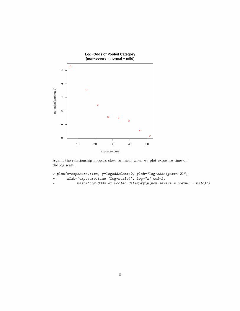
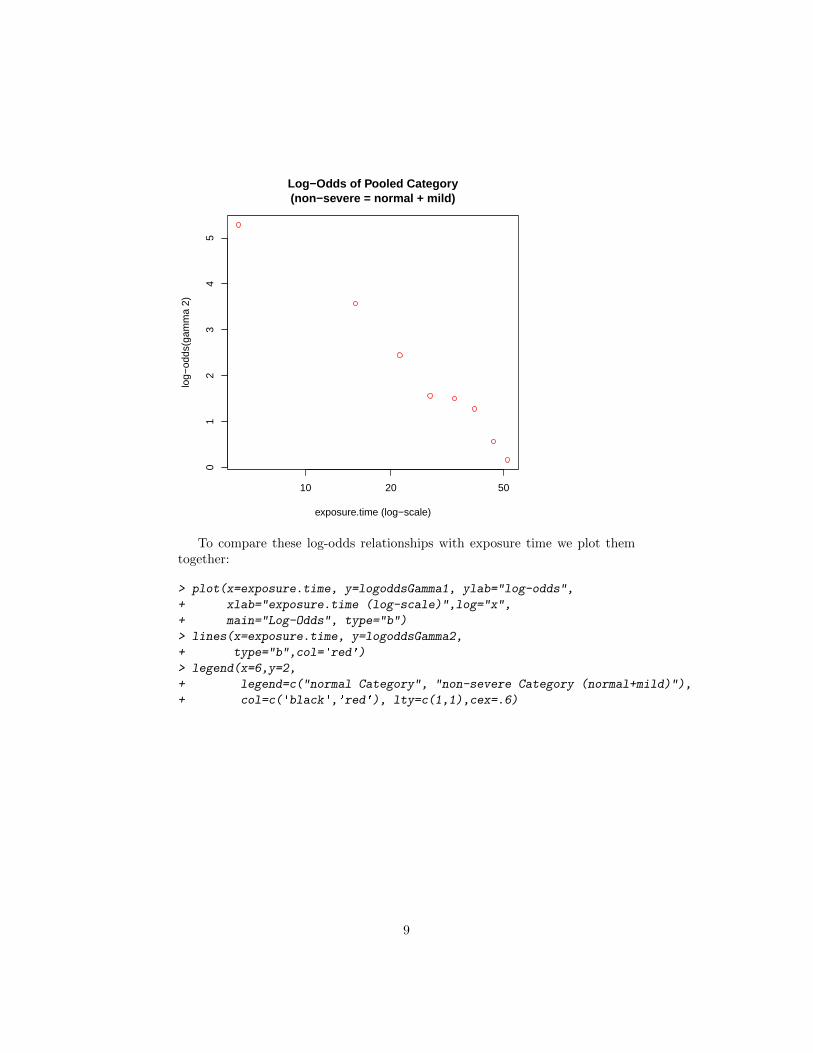
10 20 50
01
23
45
LogminusOdds
exposuretime (logminusscale)
logminus
odds
normal Categorynonminussevere Category (normal+mild)
10
---
13 Proportional Odds Model Parallel Linear Logit Model
McCullagh and Nelder comment that these plots of the transformed variables suggest considering the model
log[γij (1 minus γij )] = θj minus β log ti j = 1 2 i = 1 8 Yeersquos (2010) R-package VGAM (Vector Generalized Linear and Additive Modshyels) provides the function vglm() to fit this model
gt pneumo lt- transform(pneumo logexpostime = log(exposuretime)) gt fit1lt-vglm(cbind(normal mild severe) ~ logexpostime + cumulative(reverse=FALSE parallel=TRUE)data = pneumo)
The R object fit1 (a class vglm object) provides details of the fitted genershyalized linear model First print a summary of the fit
gt summary(fit1)
Call vglm(formula = cbind(normal mild severe) ~ logexpostime
family = cumulative(reverse = FALSE parallel = TRUE) data = pneumo)
Pearson residuals Min 1Q Median 3Q Max
logit(P[Ylt=1]) -1248 -007164 01441 03086 07714 logit(P[Ylt=2]) -1044 -018415 03093 03353 05048
Coefficients Estimate Std Error z value Pr(gt|z|)
(Intercept)1 96761 13241 7308 272e-13 (Intercept)2 105817 13454 7865 369e-15 logexpostime -25968 03811 -6814 950e-12
Signif codes 0 0001 001 005 01 1
Number of linear predictors 2
Names of linear predictors logit(P[Ylt=1]) logit(P[Ylt=2])
Dispersion Parameter for cumulative family 1
Residual deviance 50268 on 13 degrees of freedom
Log-likelihood -250903 on 13 degrees of freedom
Number of iterations 4
Exponentiated coefficients
11
logexpostime 007451115
Important components of the summary are
bull Coefficients maximum-likelihood estimates of the model parameters In addition to the Estimates estimates of their standard deviation (Std Error) their ratio (z value) and the P-value for the (asymptotic) test of whether the underlying coefficient is zero
Note the coefficients specify the parallel lines defining the log-odds as a function of the log(exposure time)
bull Log-Likelihood minus250903 on 13 degrees of freedom
Note the degrees of freedom are the total degrees of freedom (8 times (3 minus 1)) minus the number of estimated parameters 3
bull Residual deviance (see Deviance definition in lecture notes)
To the plot of observed log-odds vs exposure-time we add the ML-Fitted log-odds according to the (parallel) cumulative log-odds model
gt plot(x=exposuretime y=logoddsGamma1 ylab=log-odds + xlab=exposuretime (log-scale)log=x + main=Log-Odds Observed and Parallel Fits type=bylim=c(min(logoddsGamma1) 6)) gt lines(x=exposuretime y=logoddsGamma2 + type=bcol=red) gt lines(exposuretime y=fit1predictors[1]type=blty=2 col=black) gt lines(exposuretime y=fit1predictors[2]type=blty=2 col=red) gt legend(x=6y=2 + legend=c(normal Category non-severe Category (normal+mild) + Fitted normal Category Fitted non-severe Category (normal+mild)) + col=c(blackredblackred) lty=c(1122)cex=6)
12
10 20 50
01
23
45
6
LogminusOdds Observed and Parallel Fits
exposuretime (logminusscale)
logminus
odds
normal Categorynonminussevere Category (normal+mild)Fitted normal CategoryFitted nonminussevere Category (normal+mild)
The vglm object fit1 includes fitted values for the multinomial probabilities These are printed out together with the observed frequencies
gt pneumorateslt-dataframe(exposuretime normal= normalmcount + mild=mildmcount severe=severemcount) gt pneumofittedrateslt-dataframe(cbind(exposuretimefit1fittedvalues)) gt print(cbind(pneumorates pneumofittedrates)digits=3)
exposuretime normal mild severe exposuretime normal mild severe 1 58 1000 0000 00000 58 0994 000356 000243 2 150 0944 0037 00185 150 0934 003843 002794 3 215 0791 0140 00698 215 0847 008509 006821 4 275 0729 0104 01667 275 0745 013364 012181 5 335 0627 0196 01765 335 0636 017615 018802 6 395 0605 0184 02105 395 0532 020558 026210 7 460 0429 0214 03571 460 0434 022078 034536 8 515 0364 0182 04545 515 0364 022202 041430
13
---
14 GeneralIndependent Linear Logit Models
The model of the previous section assumes parallel linear log-odds relationships on log exposure time A more general model allows these lines to have different slopes
The R-code below fits this model
gt pneumo lt- transform(pneumo logexpostime = log(exposuretime)) gt fit2lt-vglm(cbind(normal mild severe) ~ logexpostime + cumulative(reverse=FALSE parallel=FALSE)data = pneumo)
The R object fit2 (a class vglm object) provides details of the fitted genshyeralized linear model We print out the summary of this fit and focus on the coefficients corresponding to the slope parameters
gt summary(fit2)
Call vglm(formula = cbind(normal mild severe) ~ logexpostime
family = cumulative(reverse = FALSE parallel = FALSE) data = pneumo)
Pearson residuals Min 1Q Median 3Q Max
logit(P[Ylt=1]) -115 -01457 01249 03824 07288 logit(P[Ylt=2]) -115 -00506 01886 02864 05659
Coefficients Estimate Std Error z value Pr(gt|z|)
(Intercept)1 95933 13308 7208 566e-13 (Intercept)2 111048 18930 5866 445e-09 logexpostime1 -25713 03839 -6698 211e-11 logexpostime2 -27435 05323 -5155 254e-07
Signif codes 0 0001 001 005 01 1
Number of linear predictors 2
Names of linear predictors logit(P[Ylt=1]) logit(P[Ylt=2])
Dispersion Parameter for cumulative family 1
Residual deviance 48844 on 12 degrees of freedom
Log-likelihood -250191 on 12 degrees of freedom
Number of iterations 6
14
Exponentiated coefficients logexpostime1 logexpostime2
007643613 006434155
Important components of the summary are
bull Coefficients maximum-likelihood estimates of the model parameters In addition to the Estimates estimates of their standard deviation (Std Error) their ratio (z value) and the P-value for the (asymptotic) test of whether the underlying coefficient is zero
Note the coefficients specify two lines
logit(P [Y le 1]) = [(Intercept) 1]+[logexpostime 1]timeslog(ExposureT ime)
logit(P [Y le 2]) = [(Intercept) 2]+[logexpostime 2]timeslog(ExposureT ime)
The estimated slopes are very close minus25713 versus minus27435 and very similar to the slope of minus25968 in the first model
bull Log-Likelihood minus250191 on 12 degrees of freedom
Note the degrees of freedom are the total degrees of freedom (8 times (3 minus 1)) minus the number of estimated parameters 4 (two intercepts and two slopes)
The ML-Fitted log-odds according to this (non-parallel) cumulative log-odds model can be added to the plot given before
gt plot(x=exposuretime y=logoddsGamma1 ylab=log-odds + xlab=exposuretime (log-scale)log=x + main=Log-Odds Observed Parallel and Non-Parallel Fits + type=bylim=c(min(logoddsGamma1) 7)) gt lines(x=exposuretime y=logoddsGamma2 + type=bcol=red) gt lines(exposuretime y=fit1predictors[1]type=blty=2 col=black) gt lines(exposuretime y=fit1predictors[2]type=blty=2 col=red) gt lines(exposuretime y=fit2predictors[1]type=blty=2 col=bluelwd=2) gt lines(exposuretime y=fit2predictors[2]type=blty=2 col=greenlwd=2) gt legend(x=12y=7 + legend=c(normal Category non-severe Category (normal+mild) + Fit1 normal Category Fit1 non-severe Category (normal+mild) + Fit2 normal Category Fit2 non-severe Category (normal+mild)) + col=c(blackredblackredgreenblue) lty=c(112222) + lwd=c(111122)cex=8)
15
10 20 50
02
46
LogminusOdds Observed Parallel and NonminusParallel Fits
exposuretime (logminusscale)
logminus
odds
normal Categorynonminussevere Category (normal+mild)Fit1 normal CategoryFit1 nonminussevere Category (normal+mild)Fit2 normal CategoryFit2 nonminussevere Category (normal+mild)
This plot demonstrates that model fit2 with independent linear logit funcshytions is very close to model fit1 with parallel linear logit functions
15 Likelihood-Ratio Test of Proportional Odds
We use the V GAM -package function lrtest vglm to conduct a likelihood ratio test comparing the two models
gt lrtest_vglm(fit2fit1)
Likelihood ratio test
Model 1 cbind(normal mild severe) ~ logexpostime Model 2 cbind(normal mild severe) ~ logexpostime Df LogLik Df Chisq Pr(gtChisq)
1 12 -25019 2 13 -25090 1 01424 07059
gt
Note that the likelihood ratio test statistic is LR minus Statistic = minus2 times (Log minus likelihood[fit1] minus Log minus Likelihood[fit2])
= minus2 times (minus250903 minus [minus250191]) = minus2 times (+0712) = +1424
16
Under the null hypothesis of no improvement allowing the slopes of the log-odds functions to be different the statistic is asymptotically distributed as a Chi-Square random variable with degrees of freedom equal to the difference in degrees of freedom of the two models (1 in this case) The large P-Value (07059 gtgt 005) indicates that improvement of model fit2 over model fit1 is not statistically significant
16 References
Ashford (1959) An Approach to the analysis of data for semi-quantal responses in biological assay Biometrics 15 573-81
McCullagh and Nelder (1989) Generalized Linear Models 2nd Ed Chapman and Hall New York
Yee T W (2010) The VGAM package for categorical data analysis Journal of Statistical Software 32 1-34 httpwwwjstatsoftorgv32i10
17
MIT OpenCourseWarehttpocwmitedu
18655 Mathematical StatisticsSpring 2016
For information about citing these materials or our Terms of Use visit httpocwmiteduterms

---
13 Proportional Odds Model Parallel Linear Logit Model
McCullagh and Nelder comment that these plots of the transformed variables suggest considering the model
log[γij (1 minus γij )] = θj minus β log ti j = 1 2 i = 1 8 Yeersquos (2010) R-package VGAM (Vector Generalized Linear and Additive Modshyels) provides the function vglm() to fit this model
gt pneumo lt- transform(pneumo logexpostime = log(exposuretime)) gt fit1lt-vglm(cbind(normal mild severe) ~ logexpostime + cumulative(reverse=FALSE parallel=TRUE)data = pneumo)
The R object fit1 (a class vglm object) provides details of the fitted genershyalized linear model First print a summary of the fit
gt summary(fit1)
Call vglm(formula = cbind(normal mild severe) ~ logexpostime
family = cumulative(reverse = FALSE parallel = TRUE) data = pneumo)
Pearson residuals Min 1Q Median 3Q Max
logit(P[Ylt=1]) -1248 -007164 01441 03086 07714 logit(P[Ylt=2]) -1044 -018415 03093 03353 05048
Coefficients Estimate Std Error z value Pr(gt|z|)
(Intercept)1 96761 13241 7308 272e-13 (Intercept)2 105817 13454 7865 369e-15 logexpostime -25968 03811 -6814 950e-12
Signif codes 0 0001 001 005 01 1
Number of linear predictors 2
Names of linear predictors logit(P[Ylt=1]) logit(P[Ylt=2])
Dispersion Parameter for cumulative family 1
Residual deviance 50268 on 13 degrees of freedom
Log-likelihood -250903 on 13 degrees of freedom
Number of iterations 4
Exponentiated coefficients
11
logexpostime 007451115
Important components of the summary are
bull Coefficients maximum-likelihood estimates of the model parameters In addition to the Estimates estimates of their standard deviation (Std Error) their ratio (z value) and the P-value for the (asymptotic) test of whether the underlying coefficient is zero
Note the coefficients specify the parallel lines defining the log-odds as a function of the log(exposure time)
bull Log-Likelihood minus250903 on 13 degrees of freedom
Note the degrees of freedom are the total degrees of freedom (8 times (3 minus 1)) minus the number of estimated parameters 3
bull Residual deviance (see Deviance definition in lecture notes)
To the plot of observed log-odds vs exposure-time we add the ML-Fitted log-odds according to the (parallel) cumulative log-odds model
gt plot(x=exposuretime y=logoddsGamma1 ylab=log-odds + xlab=exposuretime (log-scale)log=x + main=Log-Odds Observed and Parallel Fits type=bylim=c(min(logoddsGamma1) 6)) gt lines(x=exposuretime y=logoddsGamma2 + type=bcol=red) gt lines(exposuretime y=fit1predictors[1]type=blty=2 col=black) gt lines(exposuretime y=fit1predictors[2]type=blty=2 col=red) gt legend(x=6y=2 + legend=c(normal Category non-severe Category (normal+mild) + Fitted normal Category Fitted non-severe Category (normal+mild)) + col=c(blackredblackred) lty=c(1122)cex=6)
12
10 20 50
01
23
45
6
LogminusOdds Observed and Parallel Fits
exposuretime (logminusscale)
logminus
odds
normal Categorynonminussevere Category (normal+mild)Fitted normal CategoryFitted nonminussevere Category (normal+mild)
The vglm object fit1 includes fitted values for the multinomial probabilities These are printed out together with the observed frequencies
gt pneumorateslt-dataframe(exposuretime normal= normalmcount + mild=mildmcount severe=severemcount) gt pneumofittedrateslt-dataframe(cbind(exposuretimefit1fittedvalues)) gt print(cbind(pneumorates pneumofittedrates)digits=3)
exposuretime normal mild severe exposuretime normal mild severe 1 58 1000 0000 00000 58 0994 000356 000243 2 150 0944 0037 00185 150 0934 003843 002794 3 215 0791 0140 00698 215 0847 008509 006821 4 275 0729 0104 01667 275 0745 013364 012181 5 335 0627 0196 01765 335 0636 017615 018802 6 395 0605 0184 02105 395 0532 020558 026210 7 460 0429 0214 03571 460 0434 022078 034536 8 515 0364 0182 04545 515 0364 022202 041430
13
---
14 GeneralIndependent Linear Logit Models
The model of the previous section assumes parallel linear log-odds relationships on log exposure time A more general model allows these lines to have different slopes
The R-code below fits this model
gt pneumo lt- transform(pneumo logexpostime = log(exposuretime)) gt fit2lt-vglm(cbind(normal mild severe) ~ logexpostime + cumulative(reverse=FALSE parallel=FALSE)data = pneumo)
The R object fit2 (a class vglm object) provides details of the fitted genshyeralized linear model We print out the summary of this fit and focus on the coefficients corresponding to the slope parameters
gt summary(fit2)
Call vglm(formula = cbind(normal mild severe) ~ logexpostime
family = cumulative(reverse = FALSE parallel = FALSE) data = pneumo)
Pearson residuals Min 1Q Median 3Q Max
logit(P[Ylt=1]) -115 -01457 01249 03824 07288 logit(P[Ylt=2]) -115 -00506 01886 02864 05659
Coefficients Estimate Std Error z value Pr(gt|z|)
(Intercept)1 95933 13308 7208 566e-13 (Intercept)2 111048 18930 5866 445e-09 logexpostime1 -25713 03839 -6698 211e-11 logexpostime2 -27435 05323 -5155 254e-07
Signif codes 0 0001 001 005 01 1
Number of linear predictors 2
Names of linear predictors logit(P[Ylt=1]) logit(P[Ylt=2])
Dispersion Parameter for cumulative family 1
Residual deviance 48844 on 12 degrees of freedom
Log-likelihood -250191 on 12 degrees of freedom
Number of iterations 6
14
Exponentiated coefficients logexpostime1 logexpostime2
007643613 006434155
Important components of the summary are
bull Coefficients maximum-likelihood estimates of the model parameters In addition to the Estimates estimates of their standard deviation (Std Error) their ratio (z value) and the P-value for the (asymptotic) test of whether the underlying coefficient is zero
Note the coefficients specify two lines
logit(P [Y le 1]) = [(Intercept) 1]+[logexpostime 1]timeslog(ExposureT ime)
logit(P [Y le 2]) = [(Intercept) 2]+[logexpostime 2]timeslog(ExposureT ime)
The estimated slopes are very close minus25713 versus minus27435 and very similar to the slope of minus25968 in the first model
bull Log-Likelihood minus250191 on 12 degrees of freedom
Note the degrees of freedom are the total degrees of freedom (8 times (3 minus 1)) minus the number of estimated parameters 4 (two intercepts and two slopes)
The ML-Fitted log-odds according to this (non-parallel) cumulative log-odds model can be added to the plot given before
gt plot(x=exposuretime y=logoddsGamma1 ylab=log-odds + xlab=exposuretime (log-scale)log=x + main=Log-Odds Observed Parallel and Non-Parallel Fits + type=bylim=c(min(logoddsGamma1) 7)) gt lines(x=exposuretime y=logoddsGamma2 + type=bcol=red) gt lines(exposuretime y=fit1predictors[1]type=blty=2 col=black) gt lines(exposuretime y=fit1predictors[2]type=blty=2 col=red) gt lines(exposuretime y=fit2predictors[1]type=blty=2 col=bluelwd=2) gt lines(exposuretime y=fit2predictors[2]type=blty=2 col=greenlwd=2) gt legend(x=12y=7 + legend=c(normal Category non-severe Category (normal+mild) + Fit1 normal Category Fit1 non-severe Category (normal+mild) + Fit2 normal Category Fit2 non-severe Category (normal+mild)) + col=c(blackredblackredgreenblue) lty=c(112222) + lwd=c(111122)cex=8)
15
10 20 50
02
46
LogminusOdds Observed Parallel and NonminusParallel Fits
exposuretime (logminusscale)
logminus
odds
normal Categorynonminussevere Category (normal+mild)Fit1 normal CategoryFit1 nonminussevere Category (normal+mild)Fit2 normal CategoryFit2 nonminussevere Category (normal+mild)
This plot demonstrates that model fit2 with independent linear logit funcshytions is very close to model fit1 with parallel linear logit functions
15 Likelihood-Ratio Test of Proportional Odds
We use the V GAM -package function lrtest vglm to conduct a likelihood ratio test comparing the two models
gt lrtest_vglm(fit2fit1)
Likelihood ratio test
Model 1 cbind(normal mild severe) ~ logexpostime Model 2 cbind(normal mild severe) ~ logexpostime Df LogLik Df Chisq Pr(gtChisq)
1 12 -25019 2 13 -25090 1 01424 07059
gt
Note that the likelihood ratio test statistic is LR minus Statistic = minus2 times (Log minus likelihood[fit1] minus Log minus Likelihood[fit2])
= minus2 times (minus250903 minus [minus250191]) = minus2 times (+0712) = +1424
16
Under the null hypothesis of no improvement allowing the slopes of the log-odds functions to be different the statistic is asymptotically distributed as a Chi-Square random variable with degrees of freedom equal to the difference in degrees of freedom of the two models (1 in this case) The large P-Value (07059 gtgt 005) indicates that improvement of model fit2 over model fit1 is not statistically significant
16 References
Ashford (1959) An Approach to the analysis of data for semi-quantal responses in biological assay Biometrics 15 573-81
McCullagh and Nelder (1989) Generalized Linear Models 2nd Ed Chapman and Hall New York
Yee T W (2010) The VGAM package for categorical data analysis Journal of Statistical Software 32 1-34 httpwwwjstatsoftorgv32i10
17
MIT OpenCourseWarehttpocwmitedu
18655 Mathematical StatisticsSpring 2016
For information about citing these materials or our Terms of Use visit httpocwmiteduterms

10 20 50
01
23
45
6
LogminusOdds Observed and Parallel Fits
exposuretime (logminusscale)
logminus
odds
normal Categorynonminussevere Category (normal+mild)Fitted normal CategoryFitted nonminussevere Category (normal+mild)
The vglm object fit1 includes fitted values for the multinomial probabilities These are printed out together with the observed frequencies
gt pneumorateslt-dataframe(exposuretime normal= normalmcount + mild=mildmcount severe=severemcount) gt pneumofittedrateslt-dataframe(cbind(exposuretimefit1fittedvalues)) gt print(cbind(pneumorates pneumofittedrates)digits=3)
exposuretime normal mild severe exposuretime normal mild severe 1 58 1000 0000 00000 58 0994 000356 000243 2 150 0944 0037 00185 150 0934 003843 002794 3 215 0791 0140 00698 215 0847 008509 006821 4 275 0729 0104 01667 275 0745 013364 012181 5 335 0627 0196 01765 335 0636 017615 018802 6 395 0605 0184 02105 395 0532 020558 026210 7 460 0429 0214 03571 460 0434 022078 034536 8 515 0364 0182 04545 515 0364 022202 041430
13
---
14 GeneralIndependent Linear Logit Models
The model of the previous section assumes parallel linear log-odds relationships on log exposure time A more general model allows these lines to have different slopes
The R-code below fits this model
gt pneumo lt- transform(pneumo logexpostime = log(exposuretime)) gt fit2lt-vglm(cbind(normal mild severe) ~ logexpostime + cumulative(reverse=FALSE parallel=FALSE)data = pneumo)
The R object fit2 (a class vglm object) provides details of the fitted genshyeralized linear model We print out the summary of this fit and focus on the coefficients corresponding to the slope parameters
gt summary(fit2)
Call vglm(formula = cbind(normal mild severe) ~ logexpostime
family = cumulative(reverse = FALSE parallel = FALSE) data = pneumo)
Pearson residuals Min 1Q Median 3Q Max
logit(P[Ylt=1]) -115 -01457 01249 03824 07288 logit(P[Ylt=2]) -115 -00506 01886 02864 05659
Coefficients Estimate Std Error z value Pr(gt|z|)
(Intercept)1 95933 13308 7208 566e-13 (Intercept)2 111048 18930 5866 445e-09 logexpostime1 -25713 03839 -6698 211e-11 logexpostime2 -27435 05323 -5155 254e-07
Signif codes 0 0001 001 005 01 1
Number of linear predictors 2
Names of linear predictors logit(P[Ylt=1]) logit(P[Ylt=2])
Dispersion Parameter for cumulative family 1
Residual deviance 48844 on 12 degrees of freedom
Log-likelihood -250191 on 12 degrees of freedom
Number of iterations 6
14
Exponentiated coefficients logexpostime1 logexpostime2
007643613 006434155
Important components of the summary are
bull Coefficients maximum-likelihood estimates of the model parameters In addition to the Estimates estimates of their standard deviation (Std Error) their ratio (z value) and the P-value for the (asymptotic) test of whether the underlying coefficient is zero
Note the coefficients specify two lines
logit(P [Y le 1]) = [(Intercept) 1]+[logexpostime 1]timeslog(ExposureT ime)
logit(P [Y le 2]) = [(Intercept) 2]+[logexpostime 2]timeslog(ExposureT ime)
The estimated slopes are very close minus25713 versus minus27435 and very similar to the slope of minus25968 in the first model
bull Log-Likelihood minus250191 on 12 degrees of freedom
Note the degrees of freedom are the total degrees of freedom (8 times (3 minus 1)) minus the number of estimated parameters 4 (two intercepts and two slopes)
The ML-Fitted log-odds according to this (non-parallel) cumulative log-odds model can be added to the plot given before
gt plot(x=exposuretime y=logoddsGamma1 ylab=log-odds + xlab=exposuretime (log-scale)log=x + main=Log-Odds Observed Parallel and Non-Parallel Fits + type=bylim=c(min(logoddsGamma1) 7)) gt lines(x=exposuretime y=logoddsGamma2 + type=bcol=red) gt lines(exposuretime y=fit1predictors[1]type=blty=2 col=black) gt lines(exposuretime y=fit1predictors[2]type=blty=2 col=red) gt lines(exposuretime y=fit2predictors[1]type=blty=2 col=bluelwd=2) gt lines(exposuretime y=fit2predictors[2]type=blty=2 col=greenlwd=2) gt legend(x=12y=7 + legend=c(normal Category non-severe Category (normal+mild) + Fit1 normal Category Fit1 non-severe Category (normal+mild) + Fit2 normal Category Fit2 non-severe Category (normal+mild)) + col=c(blackredblackredgreenblue) lty=c(112222) + lwd=c(111122)cex=8)
15
10 20 50
02
46
LogminusOdds Observed Parallel and NonminusParallel Fits
exposuretime (logminusscale)
logminus
odds
normal Categorynonminussevere Category (normal+mild)Fit1 normal CategoryFit1 nonminussevere Category (normal+mild)Fit2 normal CategoryFit2 nonminussevere Category (normal+mild)
This plot demonstrates that model fit2 with independent linear logit funcshytions is very close to model fit1 with parallel linear logit functions
15 Likelihood-Ratio Test of Proportional Odds
We use the V GAM -package function lrtest vglm to conduct a likelihood ratio test comparing the two models
gt lrtest_vglm(fit2fit1)
Likelihood ratio test
Model 1 cbind(normal mild severe) ~ logexpostime Model 2 cbind(normal mild severe) ~ logexpostime Df LogLik Df Chisq Pr(gtChisq)
1 12 -25019 2 13 -25090 1 01424 07059
gt
Note that the likelihood ratio test statistic is LR minus Statistic = minus2 times (Log minus likelihood[fit1] minus Log minus Likelihood[fit2])
= minus2 times (minus250903 minus [minus250191]) = minus2 times (+0712) = +1424
16
Under the null hypothesis of no improvement allowing the slopes of the log-odds functions to be different the statistic is asymptotically distributed as a Chi-Square random variable with degrees of freedom equal to the difference in degrees of freedom of the two models (1 in this case) The large P-Value (07059 gtgt 005) indicates that improvement of model fit2 over model fit1 is not statistically significant
16 References
Ashford (1959) An Approach to the analysis of data for semi-quantal responses in biological assay Biometrics 15 573-81
McCullagh and Nelder (1989) Generalized Linear Models 2nd Ed Chapman and Hall New York
Yee T W (2010) The VGAM package for categorical data analysis Journal of Statistical Software 32 1-34 httpwwwjstatsoftorgv32i10
17
MIT OpenCourseWarehttpocwmitedu
18655 Mathematical StatisticsSpring 2016
For information about citing these materials or our Terms of Use visit httpocwmiteduterms

MIT OpenCourseWarehttpocwmitedu
18655 Mathematical StatisticsSpring 2016
For information about citing these materials or our Terms of Use visit httpocwmiteduterms