case study: building a hybridized collaborative filtering
TRANSCRIPT

Case Study: Building a Hybridized Collaborative Filtering Recommendation Engine
A technical paper of how Rue La La built a personalized shopping experience with Databricks
Guest contributors: Ben Wilson, Data Science Architect at Rue La La and Stephen Harrison, Architect at Rue La La

In the middle of 2017, an initiative began throughout the company to bring a personalized shopping experience to Rue La La. Based on preliminary research into bringing recommendations to the site and app, the prevailing opinion was that we could realize a lift in sales and engagement in the high single digits. The company was aware that bringing this to customers would require some form of Data Science, but it was a realm that none had dealt with before. We, a newly hired group of Data Scientists, Software Engineers, and Data Engineers, had all come from myriad backgrounds in Engineering, consulting, finance, and manufacturing, and as such had no experience with building a recommendation engine, let alone knowing what one is other than our own experience with them as customers of other sites. We quickly began our research into white papers, engineering blog posts, and digging into available models that could help us solve the problem.
What we found was two primary issues: firstly, the number of users and products that we needed to provide recommendations for was quite substantial and would require a large memory footprint to run; secondly, because we are a flash sale site, upwards of 40% of our products on our site and app have a cold-start problem. We knew that we needed a service to run this model on that could handle extremely large data sets, was easy to develop in, as well as having the capability to handle complex operations in-memory for creating denormalized data sets that could be fed to an on-demand API. Due to the nature of the business, we also needed a service that could flexibly
scale to increases in both customers and products without having to invest in architecture modifications to support the transient seasonality of retail.
To commence the project, we assembled a large cross-functional team consisting of front-end developers, back-end developers, an architect, and a data scientist. We knew from the start that we would have to provide the data in a manner that would allow data access that could serve a sub-40 ms response time, and that the entire payload of recommendations would need to be able to be served in a single REST request. This meant that a complex JSON payload structure would need to be engineered in the post-processing phase from the model output before being exported to a data service capable of storing the payload.
We did not choose to develop the input to the recommendation service on the Databricks Unified Analytics Platform solely because it has a robust Collaborative Filtering model in Apache Spark™. Nor did we choose it for its ability to run transformations on incredibly large and complex data sets, allowing us to pre-format the data in such a way that we would not have to incur extensive and expensive data manipulation tasks in another service or platform. We chose Databricks because it can do all of these things in a fully managed, auto-scaling service that allows us to execute the job quickly in a single code base on a resilient service. The service that Databricks offers is precisely the type of service that one is always looking for: one that you don’t even realize is there because it just works consistently.
About
Rue La La is a leading heavily discounted flash sale fashion website and mobile app platform that provides access to exclusive deals from top brands in the fashion industry. With more than 20 million customers and a distinctive experience with curated boutique shopping, private member-only deals, and new personalization technologies, it delivers a unique and engaging experience unlike any other e-retailer platform.
Background
2

The Project - MyRue
To begin to realize the design for MyRue, we knew we had to leverage machine learning techniques to provide a 100% customized daily feed of unique items for our active members. We wanted to focus on grouping recommendations not only based on their highest predicted affinities to groups of products, but within specific product categories (e.g. “Work Dresses for you”, “Suits you might like”). There was also a desire to provide customized recommendations within the brands that each user has the highest predicted affinity (e.g. “Nike clothes and shoes you might like”). The initial phase of work involved understanding how to leverage the ALS (alternating least squares) powered collaborative filtering (CF) implementation available within the Apache Spark MLlib package. A core component to leveraging this is to understand how to appropriately score implicit feedback within our ecosystem, as well as how to leverage the knowledge-based systems that we have created regarding what distinct behavior certain customers have that differentiate them from one another en-masse.
Rue La La is not a static-inventory site, unlike many competing e-retailers in the fashion space. Rather, it is a highly volatile inventory flash sale company, meaning that products are only available for a short time period with limited inventory quantities available to customers. Each day we experience anywhere from a 20% to 40% overhaul in available products (at 11am EST, roughly 1/3
of the site is taken ‘off sale’ and a comparative number of products are brought live). Many of the products shown are brand new (zero exposure to customers up until that point). This means that calculating affinities for total historic inventory is not only inefficient, but runs the risk of having a single customer’s recommendations for the day of active to-sell inventory be completely unavailable for sale. Because of this, we must only run predictions of affinity to the products that are scheduled to sell on a given day. We must therefore not only restrict the elements that are output for predictions, but we must also run both the model and the predictions each day to cover not only what is available to sell currently on site, but what is projected to ‘go live’ in the next 24 hours (we have product releases at 11am, 3pm, and 8pm daily).
The brand new products hitting the site at a rate of 10 to 40% of total items creates a complicated issue, whereby utilizing a SKU-based recommendation system would render these new products with no implicit feedback scores, thereby preventing predictions for them. This cold-start problem is a particularly complicated one to solve for many recommendation engines, but the sheer volume of new products that arrive on site each day means that we had to come up with an alternative to SKU-based recommendations. We had to look at product groupings and predicted probability of popularity for new items in order to rank the items within categories.
3

Categorizing Products
The general design of the site and app focuses on featuring human-curated collections of products (Boutiques) that follow a distinct theme designed to appeal to our customer base. However, the sheer volume of products that are available within the 60+ Boutiques each day makes it difficult for non-browser-type shoppers to find items that they may be looking for. There is a concept of shopping by category on the site (Category Navigation), but due to the massive skew in our inventory, certain collections of products can prove daunting to navigate.
Scrolling through 14,588 Dresses and Skirts might take awhile...
... hours, one might say...
4

Categorizing Products
In order to put collections of products that are actually relevant to individual members in front of them, a means of determining what is most relevant to them was needed. Utilizing a priori methodologies were a possibility, but this approach proved to be an incredible challenge, due to the sheer volume of some product categories of data; furthermore, only showing customers the very things that they’ve bought before provides no opportunity of discovery and fundamentally restricts the potential of a recommendation engine. We wanted an implementation to increase customer engagement (showing them products that we ‘know’ they like), increase sales (showing them products that we ‘think’ they will buy from a subjective and monetary value point), and increase retention. Implementation was to focus on having a highly dynamic recommendation engine that adapts to our flash business model: showing new deals in the product groups that they have affinities for in a highly dynamic way. All of these requirements led us to use collaborative filtering at the core of this implementation, with hybridizing of the outputs of the model to methods that enhance our business model.
For a pure CF-powered product-level recommendation engine to work, we would need to have a relatively static inventory that has a consistent amount of products that could be guaranteed to be available over periods of time longer than two or three days. For our historic input data, the fact that of the many millions of products that could potentially be in the model, no more than 60,000 products are available to sell at any given time. Likewise, entire collections of products are not available (e.g., a flash sale in women’s jeans might only be available from Tuesday to Thursday, with Friday having no jeans available onsite at all). With new inventory coming to the site each day and a steady stream of new brand and product type combinations coming in, we needed to discover a product grouping strategy that worked for our business. We decided that in order to make this recommendation engine work, we had to develop a custom hierarchy of our products that serves the function of grouping products in a logical fashion for the purposes of clustering products by use and application. Hierarchies exist within the business for several different use cases (as well as a site-displayed hierarchy that is optimized for navigation), but all of these hierarchies had either circular references, fragmented tree structures, or isolated products that are fundamentally similar to one another based on subjective reasons. After creating this hierarchy that each individual product could be assigned to, we concatenated each product’s hierarchy with the brand that made the product, thereby giving us an item primary key (which we ended up calling the subclass_brand_pk). Armed with this hierarchy, we were able to logically group types of items together for processing later on when building the product-level data set that is surfaced through the API to the app.
5

Categorizing Products
There are implementations of recommendation systems that, in theory, could more accurately pinpoint a user’s affinities to attributes of products. Many of these engines ( Pandora’s Music Genome Project, most notably) rely on a content-based recommendation system that has the possibility of being far more accurate for detecting and predicting individual tastes at a user level, and with the trove of feature data associated with a product, would allow for highly customized recommendations of high relevancy. The primary downside of these systems is that they require extensively standardized data that has been vetted and is tightly quality controlled. Deviations from standards, errors in classification, human labeling creativity, as well as the sheer amount of time and resources required to implement a product labeling initiative of this nature would be prohibitively expensive for our company to implement. The sheer number of features that we would have to generate would be staggering for the scale of products that we sell. Similarly, relying on vendor-supplied data from an industry that has few agreed-upon standards regarding definitions, terminology, and constancy would result in an endless process of perpetual QA and re-labeling.
For instance, take this dress:
The attributes that might describe the style of it could include the dress length, sleeve length, neckline, pattern, overall shape, back type, waist type, and a subjective style classification. Ensuring that the labels applied to this example are consistent with all other dresses that are available to sell currently, as well as historically, would require a level of subjective and objective standardization that is simply untenable.
It is for this reason primarily that we chose to go with a content-agnostic modeling approach that requires no additional data to explain the products other than user activity to items that are grouped together in the hierarchy family. In this example, that would be:
Division: Women’s Department: Clothes Class: Dresses Subclass: Day Dress
Why Collaborative Filtering?
6

Categorizing Products
Had we the time and resources available to get accurate and consistent feature labels on this dress (and all other 1,000,000 + items in our historic catalog), we might have something that looks like this:
Dress Length: Mid Thigh Sleeve Length: Half Neckline: Collared Pattern: Paisley Color: Teal / Burgundy Shape: Shift Back Type: Closed Shoulders: Full Waist Type: Fitted Style: Traditional Occasion: Work Casual
Giving another style expert the image of that dress, we would undoubtedly get different answers about that dress above and the classifications provided. In point of fact, we actually have done this very experiment with stylist experts within the company, and unfortunately, a quorum of majority-ruled labeling cannot be achieved on a single product among a group of 7 experts (particularly on subjective measures such as ‘style’ and ‘occasion’). Due to the highly subjective nature of fashion, being so heavily influenced by personal bias, it is nigh impossible to build a content-based recommendation system with our business model.
Luckily, with a collaborative filtering model, the only thing we need to know is the fact that the item shown above is a Day Dress, as well as its brand, and we can group interactions with this group of products on a per-member basis to determine what a user’s affinities are, as well as what they are likely to buy based on similar user’s behaviors.
7

Categorizing Products
Most contemporary implementations of recommendation engines that do not rely on highly curated and standardized attributes of products utilize a form of matrix factorization in order to determine predicted affinities for items (or, in our case, groups of items) on a per-member basis.
There are 3 inputs to the ALS model in Apache Spark: User_ID (an integer representing the primary key assigned to each member of the site) Item_ID (in our case, due to the flash model, the subclass_brand_pk that groups of products fall under) Implicit Rating (a score associated with a User’s interaction with an Item) / Explicit Rating (a score associated with a User’s rating of an Item)
For the implementation at Rue La La, we’ve gone with using an Implicit Rating system (with customized scoring methodology), since we do not have the ability to retrieve explicit ratings on our goods from our members.
For a full description on how we’re leveraging implicit feedback with ALS Collaborative Filtering, see the foundational paper here.
How we handle Implicit RatingsOne of the challenges of determining if a member ‘likes’ something or not is buried within our site activity feed data (clickstream), our order system, and our still-want-it program (due to our flash-sale business model, products are frequently sold out due to low inventory and high popularity of certain items). The architecture of our website and mobile apps has a tiered hierarchy of interaction with collections of products (Boutiques, consisting of a representative art-style image that captures the essence of the products that are contained within the product grouping), product list pages (PLP, which is a view-able collection of products in a scrollable list), product display pages (PDP, a one-item page from which items can be viewed in more detail, added to a checkout cart, or directly purchased in some cases), the cart (collected items can be purchased from here provided that they are still in stock), a still-want-it option (SWI, wherein a customer can declare that even though the product is out of stock, that if an order is cancelled by someone else who reserved it, or if more stock comes in, they can then purchase the item directly), and a purchase confirmation event. Although we collect far more information about member behavior than those 4 elements, we found through experimentation and testing that a solid predictive model could be developed by using these 4 primary data sources.
What is the collaborative filtering model?
8

Categorizing Products
Due to the fact that there is no information to be gained at the Boutique level (or the product list page level, for that matter), the first entry point that we can use to identify an affinity to a product is at the product display page. Our scoring from that point of interaction is as follows:
If a member clicks on an item shown on the PLP that then takes them to a PDP, we count that event and assign it 3 ‘points’. If a member then adds that item to their card, we count that and assign that event 10 ‘points’. If a member attempts to buy something that is currently sold out through the ‘still want it’ feature, then that receives 30 ‘points’. If a member makes a purchase, then we attribute that with 40 ‘points’.
For each member’s viewing and purchase history, we then aggregate and sum all activity for each member under the subclass-brand level that they have interacted with. This gives us the input dense vector of the user, item, rating (implicit) in the form of (MEMBER_ID, SUBCLASS_BRAND_PK, RATING)
How Collaborative Filtering worksAt its core, matrix factorization is trying to fill in missing data. In our case, for this recommendation engine, the model is effectively processing a matrix of users by items, cells being filled with implicit ratings of the items for each user:
This matrix is relatively sparse (empty) since the vast majority of users will not have interactions with every single item.
Item_1 Item_2 Item_3 Item_4 Item_5 Item_6 Item_7 ... Item_nUser_1 12 118 19User_2 12 90User_3 15 120User_4 53
User_5 106 15User_6 468User_7 15...User_n
9

Categorizing Products
The intent of collaborative filtering is to discover the latent factors (K) for each item and each user. These resultant matrices are of the form:
User_Latent_Factor_1 User_Latent_Factor_2 ... User_Latent_Factor_n
User_1
User_2
User_3
User_4
User_5
User_6
User_7
...
User_n
Item_1 Item_2 Item_3 Item_4 Item_5 Item_6 Item_7 ... Item_n
Item_Latent_
Factor_1Item_Latent_
Factor_2...
Item_Latent_
Factor_n
10

Categorizing Products
Due to the fact that customers 1, 2, 3 all have some degree of affinity to Handbags_Brand_A, as well as customers 1 and 3 having affinities to Day_Dresses_Brand_C, it stands to reason that customer 2 will have a relatively high affinity to Day_Dresses_Brand_C, explained by the latent relationship among these customers proclivities. Due to the fact that Customer 2 shares affinities with customers 1 and 3 in Handbags from Brand_A, as well as sharing affinity with customer 3 in Handbags from Brand_B, a latent factor describing the relationships between these users would be discovered that maps their behavioral patterns similar to one another once the act of solving for the matrices is complete. On the output level after transformation of the data set with the dot product of the user and item matrices, the affinities may look something like this:
What you may notice is that all of the missing data has been filled in with predicted probabilities of affinity based on the magnitude of the per-member implicit feedback, as well as the latent factors that describe the customers relationships to one another (customer 1 has a predicted affinity for Handbags_Brand_B, for instance, as well as for Hats_Brand_B due to the fact that customers 2 and 3 also had affinities to these).
Customer Handbags_Brand_A
Handbags_Brand_B
Day_Dresses_Brand_A
Day_Dresses_Brand_C
Hats_Brand_A
Hats_Brand_B
1 520 245
2 120 50 400
3 200 500 150
Customer Handbags_Brand_A
Handbags_Brand_B
Day_Dresses_Brand_A
Day_Dresses_Brand_C
Hats_Brand_A
Hats_Brand_B
1 0.995 0.9 0.0 0.92 0.0 0.8
2 0.9 0.85 0.0 0.92 0.0 0.995
3 0.99 0.995 0.0 0.95 0.0 0.9
What are latent factors?A latent factor (or latent variable) refers to influences to events that are not directly observable. They are the ‘hidden connections’ within observable data that can be inferred mathematically based on common relationships that exist. For the case of Collaborative filtering, let’s take a moment to explain this through a simplified data set.
Suppose that we have 3 customers with the following activity scores:
11

Categorizing Products
In traditional implementations of collaborative filtering (prior to ALS), in order to solve the matrices of user latent factors and item latent factors, the matrix factorization had to be solved by inverting the input matrix and solving for the latent factors through SVD, which is incredibly memory and computationally expensive for large data sets. Although it is technically more correct and exacting, the gain in accuracy does not outweigh the speed and resource gains by using ALS on Spark.
Spark’s implementation of ALS involves randomly initializing the user latent factor matrix, holding it constant, and solving for the item latent factor matrix. On the next iteration (influenced by the regularization Parameter value to prevent over-fitting), the item latent factor matrix is held constant, and the user latent factor matrix is solved for. This process continues until optimization of both matrices meets the approximation of the input matrix set as best as possible.
The implementation of ALS allows for these operations to be conducted in parallel, speeding up convergence by many orders of magnitude. By increasing the number of EC2 nodes in the Spark cluster and optimizing the block counts for parallel operations, we can effectively tune the model building time without sacrificing recommendation quality, while speeding up the processing time to reduce costs and prevent delays in serving up daily recommendations.After having both of these matrices, we can then get a recommendation for a user by taking the dot product of the user latent factor matrix and the item latent factor matrix to get a predicted affinity for a user (or for an item).
What is special about ALS on Spark
12

Categorizing Products
Let’s tackle this as a list:
• It’s a fully managed service.• We don’t have a team of OPS specialists working with us. Although many people on the Rue Data Science team
know how to manage cloud-based servers, can configure Spark to run on an EC2 machine, and can troubleshoot configuration problems, it’s simply just a massive time-sink to have software engineers and data scientists messing about with environment configurations and monitoring YARN. With Databricks, we don’t have to worry about our environment. When we start developing for a new project, it takes about 30 seconds to define a dev environment, load packages, and start coding.
• It’s flexible. • We have a few dozen jobs running on Databricks now, some using functional Scala code, other using object-
oriented packages, and some with embedded SQL. With Databricks, we can seamlessly move from one to the other (even within the same job!).
• It’s fast. • Not just in the execution time (I’m sure it’s comparable to managing your own servers), but more so in
development time. We can rapidly prototype code, view and manipulate results from within the development environment, synchronize to GitHub, push a QA version of the code, and set up a production schedule and job in a fraction of the time than if we were using anything else. We can do all of this on a single unified platform with a robust API toolkit that allows us to do everything from rapid prototyping to a full CI/CD stack implementation of a production service.
• It plays well with others. • Our data warehouse / data lake services can be directly connected to from Databricks. Since we use Snowflake as
our primary data source for accessing all information about our members and products, it is seamless to directly connect to our data warehouse, directly import to Spark without any time-consuming ETL processes, and write back to Snowflake directly. We’re also able to directly connect to our site activity feeds (Kinesis stream) to create custom data sets that can be evaluated in real-time (< 1-second delay from user activity to data output).
But why Databricks over the competition?
13

Explanation of model hyper-parameters
Within Spark’s implementation of Collaborative Filtering, the model can be tuned by several hyper-parameters which all affect either the time of execution or the quality of the recommendations.
numBlocks: the number of blocks that users will be partitioned into in order to parallelize the computation to find latent factors within the user and item matrices.
rank: the number of latent factors in the model (default: 10)maxIter: the maximum number of iterations to run (default: 10)
regParam: the regularization parameter for ALS to determine whether or not an iteration of least squares optimization reduces or increases least squares estimation of latent factors contributing to an accurate fit. (prevents over-fitting, but slows the learning rate)
implicitPrefs: specification of whether or not to use explicit or implicit feedback. (default: false(explicit))
alpha: for implicit usage only, it governs the baseline confidence in preference observations (default: 1.0) (this is particularly useful when assigning ordinal counts of activities without weighting individual implicit factors on the activity type being measured)
For the roll-out of full member-launch of MyRue initially, the base settings for the model are: numBlocks: (see below for explanation) rank: 50 maxIter: 10 regParam: 0.01 implicitPrefs: true alpha: 0.05
The vast majority of these settings were obtained through cross-validation (at first) to discover initial ‘ballpark’ values, utilizing a simple RMSE evaluator to dial-in settings to the point of lowest observed error rate. Once a general set of thresholds of settings were obtained that minimized the RMSE, we set up training and holdout data sets (through masking of implicit inputs randomly) and measured the success criteria of recommendations through a confusion matrix to determine the success rate of recommending item groups that members actually discovered and interacted with themselves. After this point, QA data sets were generated for collections of users’ (employees, as well as randomly sampled members) recommendations of particular product groupings, which were then user-acceptance-tested, empowering further model tuning to the point that we arrived at the above set points for hyper-parameters.
14

Our implementation of the Collaborative Filtering Model
When we were preparing to pursue a recommendation engine for Rue La La, we began by spending time getting to know our customers a bit better. This didn’t involve interviewing them or sending out surveys, but rather was spent in querying their behavior data; spending time aggregated and applying time-series analysis to subsets of users allowed us to gain a great deal of knowledge about how we might separate our customers into different cohorts that have isolated behavior patterns. This was particularly critical for our implementation due to the wide variety of items and brands that we sell, as well as the general nature of high-fashion e-commerce.
We found out that:
• Customers that buy expensive items in one product type category don’t necessarily buy relatively expensive items in others. (The classic case of expensive shoes and purse, but with a practical and modestly priced dress).
• Different groups of people have distinctly uniform, but isolated spending habits (customers who buy low-price bracelets and charms rarely, if ever, buy expensive men’s suits).
• Customers that buy a lot of gifts for others (or shop for a family) have extremely different spending habits to people who only buy for themselves.
• A one-time expensive purchase in one product category does not indicate that a customer only wants to see expensive items for a recommendation list.
• There is always a dominant relationship to a product Division (Men’s / Women’s / Kids / Home / Unisex accessories) for each customer.
• The assumption of registered gender to the website and app is indicative of purchase behavior (e.g. women buy women’s clothes, men buy men’s clothes) is patently false.
A discussion of our customers
15

Our implementation of the Collaborative Filtering Model
When looking at attributes about our customers, we felt it was important to understand from a statistics standpoint, what our historical product offerings have been at the company.
We found that:
• An overwhelming majority of our products are targeted to women.
• We have very limited information about our products and the hierarchies available to use (internal and customer-facing) were fragmented, of differing levels of detail, or classified incorrectly.
• Price points can be highly variable within a particular product category and brand (i.e. Brand_A sells $19.99 shoes, but it also sells $699.99 shoes).
Because of the above factors regarding our members and products, we decided to build a suite of CF models that were based on a two-level principle of member grouping. The first level was on a member’s 90th percentile of the purchase price of all of their orders.
The primary reason for using 90th percentile was to not be overly weighted by a single large-ticket purchase that a member might have made (an expensive handbag, for instance) that is a once-in-a-decade purchase that doesn’t accurately describe the member’s purchasing parity power. The extremely right-tailed distribution for most members dictates that using the 90P value gives adequate separation between groups of members, as well as grouping behavior of members into congruous buckets.
This assignment of groups based purely on 90th percentile of spend puts our members into five quantized buckets with the following distributions:
A discussion about our products
A discussion about clustering our members
16

Our implementation of the Collaborative Filtering Model
val stringSplit = udf((n:Integer) => n.toString.takeRight(1))display(memberDataIngest.withColumn(“Spend_Group”, stringSplit($”IQR10_PRICE_GROUP”)).groupBy($”Spend_Group”).
agg(count(“*”)).withColumnRenamed(“count(1)”, “Member_Count”).orderBy($”Spend_Group”))
Spend_Group 1 primarily purchases relatively inexpensive items, while group 5 spends money on the most expensive of our items. The intention of equally splitting members into close-to-equivalent count buckets is that the distribution of our products is highly right-tailed (from $19.99 women’s tops to $4999.99 watches) with the majority of the distribution in the $30 - $200 range.
The other breakthrough that we had when finding out ways to group similar behavior together was by discovering primary division affinity. The distribution for this is:
Databricks Visualization code for 90P Spend
17

Our implementation of the Collaborative Filtering Model
val stringSplitFirst = udf((n:Integer) => n.toString.take(1))display(memberDataIngest.withColumn(“Division_Affinity”, stringSplitFirst($”IQR10_PRICE_GROUP”)).groupBy($”Division_
Affinity”).agg(count(“*”)).withColumnRenamed(“count(1)”, “Member_Count”).orderBy($”Division_Affinity”))
The conversion of the Division_Affinity key to business division of products is as follows:
As can be seen in the distribution, we have an overwhelming number of members that fall into a ‘Primary Women Product’
customer group. This isn’t particularly surprising to us, but what was surprising was that even within a company that
predominantly markets to women, there are a sizeable number of valued customers whose primary purchases to the site
are for home goods (furniture, kitchen, bath, and bedding), and within that group we have some of our top-100 lifetime
spend customers.
Databricks Visualization code for Primary Division
Division_Key Division1 Women’s Products2 Men’s Products3 Kids Products4 Home Goods5 Unisex (Accessories / Travel / Gadgets)
18

Why we chose to build 25 models
When we combine the two of these distributions, we get a final break-out like this:
What this combined graph is showing is all of the 25 groups of members that we have identified as having similar behavior
patterns with division and spend. The first Integer in the IQR10_PRICE_GROUP describes the Division Affinity (e.g. 1x refers
to Women’s Division, 2x refers to Men’s Division) and the second integer refers to the Price Bucket that the member belongs
to (e.g. x1 refers to inexpensive item purchases, x5 refers to expensive items).
Separating these members from one another resulted in dramatic reduction in RMSE values, a significant gain in the NDCG
(Normalized Discounted Cumulative Gain) scores, a subjective improvement from User Acceptance Testing, and a 15% lift
in revenue in a closed AB test from a recommendation test that we conducted on our platform (personalized Boutique).
However, implementing this change required a significant overhaul to the way we were building the model and required
us to dynamically set hyper-parameters based on the data. Thankfully, Scala on Spark made that very easy to do.
19

How we handled dynamic block counts to improve recommendation quality
In order to adequately set the parallel collections of user groups to ensure that we’re optimizing the sub-populations of members during ALS (namely in the step of resolving the user latent factors), we need to dynamically detect the membership counts to each of the 25 groups identified above.
We handled that through supplying to the model runner a list of the groups that are available based on the input data set (dynamically supports scaling of the groups; for the purposes of this documentation, we’re sticking with 25) by running a distinct collect after grouping the DataFrame by the Group Membership field (IQR10_PRICE_GROUP). This collected group array is converted from a DataFrame to an RDD, which is then collected and sorted by value. See below code snippet:
Determing Groups Spark Command val groupsArray = memberData.select(col(groupingColumn)).distinct.rdd.map(r => r(0).asInstanceOf[Double]).collect().
sortWith(_<_)
Since we are using dynamic counts of users, we provide an upper and lower threshold to calculate an optimal userBlocksCount to use different factoring methods based on a Scala case match statement. If the group is considered to be ‘large’, we calculate the userBlock counts by using a large divisor, while if it is below the threshold, we use a much smaller divisor. This enabled both a performance improvement, as well as having the benefit of more accurate recommendation results in the final product.
The full modeling code for n groups of members: case class affinitySchemaStruct(MEMBER_SK: Int, SUBCLASS_BRAND_PK: Int, rating: Double, prediction: Double)
case class modelConfigParam(memberData: DataFrame, ratingData: DataFrame, groupingColumn: String, groupArray: Array[_], numberOfRecommendations: Integer, iter: Integer, alpha: Double, checkpoint: Integer, regularization: Double, userCol: String, itemCol: String, ratingCol: String, rankLvl: Integer,
20

How we handled dynamic block counts to improve recommendation quality
itemBlocks: Integer, userBlocksRatioLarge: Integer, userBlocksRatioSmall: Integer, userBlocksRatioThreshold: Integer)
def fullModelBuild(config: modelConfigParam): (DataFrame) = { // create an empty var DataFrame based on the final schema in order to write the predicted affinity data for each model to a single data set val affinitySchema: types.StructType = Encoders.product[affinitySchemaStruct].schema var affinityData: DataFrame = sqlContext.createDataFrame(sc.emptyRDD[Row], affinitySchema)
// loop through the groups, build a model and run affinity predictions. for (grp <- config.groupArray) {
// Debug statement for the current group to show which group the iterator is on println(“Current Group: “ + grp)
// create a filtered subset of members that are associated with the iterator group val memberFilter = config.memberData.filter(col(config.groupingColumn) === grp).select(config.userCol) println(“Number of members in group: “ + memberFilter.count) // dynamic check for large and small user groups to configure for potential sparseness of data val blockSizeCheck = config.userBlocksRatioThreshold match { case config.userBlocksRatioThreshold if(config.userBlocksRatioThreshold > memberFilter.count) => { println(“Employing Smaller Grouping Size of “ + config.userBlocksRatioSmall) config.userBlocksRatioSmall } case _ => { println(“Employing Larger Grouping Size of “ + config.userBlocksRatioLarge) config.userBlocksRatioLarge } } val userBlocks = math.ceil(memberFilter.count.toDouble / blockSizeCheck.toDouble).toInt println(“Number of Groups Being Created for Calculation of User Affinity: “ + userBlocks)
// join to the ratings data to only retrieve rating data for the members that belong to the iterator group val subsetData = memberFilter.join(config.ratingData, config.userCol).select(config.userCol, config.itemCol, config.ratingCol) println(“Building Model....”)
21

How we handled dynamic block counts to improve recommendation quality
// Create the ALS CF Model for this group val subsetPurchaseModel = buildALSModel(subsetData, config.iter, config.alpha, config.checkpoint, config.regularization, config.userCol, config.itemCol, config.ratingCol, config.rankLvl, config.itemBlocks, userBlocks) println(“Model Built.”) // Predict and extract the per-member predicted affinities val subsetAffinityPurchase = generatePredictionsUsers(config.userCol, config.itemCol, subsetPurchaseModel, subsetData, config.numberOfRecommendations) subsetData.createOrReplaceTempView(“ratings”) subsetAffinityPurchase.createOrReplaceTempView(“affinity”)
// union the prediction to the mutable DataFrame affinityData = affinityData.union(sqlContext.sql(s”””SELECT aff.${config.userCol}, aff.${config.itemCol}, NVL(r.${config.ratingCol},0) AS ${config.ratingCol}, aff.prediction FROM affinity aff LEFT OUTER JOIN ratings r ON aff.${config.userCol} = r.${config.userCol} AND aff.${config.itemCol} = r.${config.itemCol}”””)) } return affinityData
}
Within the above code is a method for extracting from the model the very relationships that we cared about most for our implementation of providing product-level recommendations to our members - the function generatePredictionsUsers(). This function has, at its core, a utilization of the .generateForAllUsers method within the org.apache.spark.ml.recommendation.ALSModel API. The code below demonstrates how we leverage that method, explode the recommendations column, and retain both the key and the predicted affinity, capped at the value passed into the function (recommendationLimit). Retrieving these lists of affinities to a product grouping category is needed further on for us to translate a key-grouped value (Subclass_Brand_PK) to a recommended list of products that are available to sell in the next day on our site. Due to the nature of our business, there is no guarantee that for a particular user that even within their ranked top 50 affinities will be for sale today. To handle this business model, we return the top 5000 affinities for each person. We also generate this affinity data set to be leveraged in other ways in the business (e.g. sorting the boutiques that are available on the site and the app in a 100% personalized manner).
22

How we handled dynamic block counts to improve recommendation quality
User Affinity Data Set Creation def generatePredictionsUsers(predictionKey: String, predictionValue: String, recommendationModel: org.apache.spark.ml.recommendation.ALSModel, rawData: DataFrame, recommendationLimit: Integer): (DataFrame) = { // function for building the prediction DataFrame based on constraints supplied // get the maximum count permitted based on the distinct count of the predictionValue field val maxCountValue = rawData.select(predictionValue).distinct().count.toInt val resetVal = if (maxCountValue < recommendationLimit) {“Y”} else {“N”} val primaryRecommendation = resetVal match { case “Y” => { println(s”Warning! Supplied limit value of: $recommendationLimit is higher than unique count values of: $maxCountValue !!”) recommendationModel.recommendForAllUsers(maxCountValue) } case “N” => { recommendationModel.recommendForAllUsers(recommendationLimit) } } val explodedRecommendation = primaryRecommendation.select(primaryRecommendation(predictionKey), explode(primaryRecommendation(“recommendations”))) val transposedAffinity = explodedRecommendation.select(explodedRecommendation(predictionKey), $”col”.getItem(predictionValue).alias(predictionValue), $”col”.getItem(“rating”).alias(“prediction”)) return transposedAffinity}
With the output of the above code, we retrieve a data set that looks like this:
Member_Id Subclass_Brand_PK rating prediction1 1001 210 0.999981 1489 6 0.99881 64589 210 0.9776...1894527 1002 0 0.00003
23

How we handled dynamic block counts to improve recommendation quality
With this data, spanning 25 groups of members, with a total modeled member count of ~ 2 million customers, and returning the top 5000 Subclass_Brand_PK for each member, we’re left with a sizeable data set that provides accurate predictions of affinity for each person. However, we didn’t stop there. The next step in our journey was to provide boosts to recent activity for each member that leverages the idea that people who are clicking around a particular product category but haven’t purchased anything yet are directly indicating an intention to purchase in the short-term. Because of this, we provide boosts to the predicted scores to a Subclass group (e.g. if someone has been browsing duvets 30 times over the past week but haven’t yet purchased one, the probability that serving up these products boosted higher on a recommended list of products will result in a conversion-to-buy is much higher than the raw results of the CF algorithm) for the last 10 days of browsing-but-not-purchase behavior. In order to not completely wash out the recommendations from CF, we only boost the top 3 most frequently viewed / added to cart (but not purchased) subclass elements over the last 10 days. If the criteria is not met (time-wise or view data-wise), then no boost will be applied for the member.
24
Converting from product groups to individual products
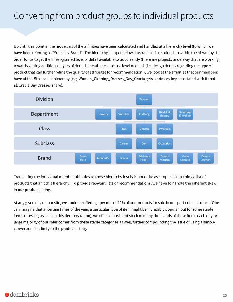
Up until this point in the model, all of the affinities have been calculated and handled at a hierarchy level (to which we have been referring as “Subclass-Brand”. The hierarchy snippet below illustrates this relationship within the hierarchy. In order for us to get the finest-grained level of detail available to us currently (there are projects underway that are working towards getting additional layers of detail beneath the subclass level of detail (i.e. design details regarding the type of product that can further refine the quality of attributes for recommendation)), we look at the affinities that our members have at this 5th level of hierarchy (e.g. Women_Clothing_Dresses_Day_Gracia gets a primary key associated with it that all Gracia Day Dresses share).
Translating the individual member affinities to these hierarchy levels is not quite as simple as returning a list of products that a fit this hierarchy. To provide relevant lists of recommendations, we have to handle the inherent skew in our product listing.
At any given day on our site, we could be offering upwards of 40% of our products for sale in one particular subclass. One can imagine that at certain times of the year, a particular type of item might be incredibly popular, but for some staple items (dresses, as used in this demonstration), we offer a consistent stock of many thousands of these items each day. A large majority of our sales comes from these staple categories as well, further compounding the issue of using a simple conversion of affinity to the product listing.
25

Converting from product groups to individual products
As an example, let’s take a look at a theoretical member’s activity and what the raw output from CF would look like:Mary is a moderately active member of Rue La La. She’s interested in dozens of product categories, ranging from dress heels to casual day dresses, kitchen gadgets to bed sheets. However, 60% of her activity has been in 4 different brands day dresses and career dresses. Because of the large volume of customers that also shop within these categories and have a high implicit affinity to multiple brands across these categories, her output from CF might look something like this:
This is all well and good; she might actually enjoy looking at all of those dresses. However, in our testing, we found that introducing affinity-backed variety to the recommendation engine led to much higher conversion rates and sales. The way that we handled enforcing variety was through implementing a simple limiting function in Spark. What this algorithm did was to enforce a limit on the number of subclass-brands that could be recommended within a single class. It would end up transforming her listing into something like this:
MemberId Subclass Brand Affinity Score1000 Gracia Day Dresses 0.9981000 Tahari ASL Day Dresses 0.9961000 Adrianna Papell Career Dresses 0.991000 Donna Morgan Day Dresses 0.921000 Adrianna Papadell Day Dresses 0.8891000 Gracia Tops 0.8731000 Gracia Skirts 0.81000 Tahari ASL Career Dresses 0.7651000 Vince Camuto Day Dresses 0.653
MemberId Subclass Brand Affinity Score1000 Gracia Day Dresses 0.9981000 Tahari ASL Day Dresses 0.9961000 Adrianna Papell Career Dresses 0.991000 Donna Morgan Day Dresses 0.921000 Gracia Tops 0.8731000 Gracia Skirts 0.81000 Tahari ASL Career Dresses 0.7651000 Prada Heels 0.7241000 Jimmy Choo Pumps 0.711
26

Converting from product groups to individual products
The output from the algorithm will, for each member, restrict the total number of subclass-brands (in this case, Day Dresses were restricted to only the top 3 brands that she has an affinity for) in order to boost variety higher while preserving the ranked affinity within each of the hierarchy positions.
The code below illustrates how we leverage a join and a windowing function in SparkSQL to return what we’re looking for:
Enforcing Variability in recommended items def rdsBoutiqueUniqueFilter(data: DataFrame, hierarchyLevelData: DataFrame, hierarchyLevelName: String, hierarchyLimitCount: Integer): DataFrame = { val dataJoin = data.join(hierarchyLevelData, “SUBCLASS_BRAND_PK”).select(“MEMBER_SK”, “SUBCLASS_BRAND_PK”, “rating”, “prediction”, hierarchyLevelName) dataJoin.createOrReplaceTempView(“levelCulling”) val cullingSQL = s””” WITH rankOrder AS ( SELECT MEMBER_SK, SUBCLASS_BRAND_PK, rating, prediction, $hierarchyLevelName, RANK() OVER (PARTITION BY (MEMBER_SK, $hierarchyLevelName) ORDER BY prediction DESC) rankedClass FROM levelCulling ) SELECT MEMBER_SK, SUBCLASS_BRAND_PK, rating, prediction FROM rankOrder WHERE rankedClass <= $hierarchyLimitCount “”” return sqlContext.sql(cullingSQL)}
In this function, we’re passing in the variable “data”, which is the modeled CF transformed output. We’re then passing in the variable “hierarchyLevelData” which is the key resolver data set that provides the normalized lookup of subclass_brand_pk to another higher level of the hierarchy (for instance, at the ‘class’ level). We pass in the name of the hierarchy level in order to provide a partitioning key to the windowing function, and finally pass in a limiting count that can be used as a tuning parameter for testing.
27

Converting from product groups to individual products
During the implementation, we didn’t see any performance differences between writing the function as SQL, rather than the alternative, pure Scala-based windowing. It is simply a more legible and easier-to-read implementation for many members of our team who come from a data engineering background (the author included).
The same function in pure Scala would be:
Alternative windowing implementation def rdsBoutiqueUniqueFilter(data: DataFrame, hierarchyLevelData: DataFrame, hierarchyLevelName: String, hierarchyLimitCount: Integer): DataFrame = { data.join(hierarchyLevelData, “SUBCLASS_BRAND_PK”) .select(“MEMBER_SK”, “SUBCLASS_BRAND_PK”, “rating”, “prediction”, hierarchyLevelName) .withColumn(“rank”, rank().over(Window.partitionBy(“MEMBER_SK”, hierarchyLevelName).orderBy(desc(“prediction”)))) .filter(col(“rank”) <= hierarchyLimitCount) .drop(col(“rank”))}
28
Generating Recommended Products
Once we achieved a reduction in the monotony of the same sort of product groupings for our members, we needed to provide a way to recommend products from what is going to be on sale over the next 24 hours. The chief difficulty in doing this is that we are a flash sale company. Due to the very nature of our business, depending on the day and time of year, we might have massive inventory available in one particular brand’s subclass grouping. For instance, there could be a Gracia sale going on during the next day wherein there are over 100 new dresses being put up for sale, 300 returning styles that we’ve had on site before but have recently acquired more inventory of, and 400 that have been on the site for the past 2 days (most products are available to buy for 72 hours only). The challenge with a large influx of new products is that our intention for selecting which products to show to customers that have an affinity to a particular product grouping is to ‘bump based on popularity’. It stands to reason that showing items that have had high purchase rate successes in the past, as well as high engagement (clicks) to them with conversions (purchases), would perform better in sales. However, this cold start problem of the 100 new dresses coming up for sale means that a pure popularity-based system would never get any visitation to the new styles. The other side of handling this is to only show the newest products first, thereby forcing freshness of product recommendations to only the newest things, regardless of historic popularity to other items.
We decided to do something between the two approaches listed above. We built a hybrid system that utilizes a system of linear equations to provide a complex scoring function based on the following factors:
1. Age of product 1. How many times have we sold this product before?2. How long has it been on site in the most recent sale?3. How persistent is this brand in this subclass category over time (i.e. do we always have some collection of Gracia dresses on site, or is this an infrequently or seasonally sourced brand?)
2. Interaction of members to product 1. How many clicks did each item get in the last n months?2. How many times was this item purchased in the last n months?3. What is the ratio of clicks to purchases?4. How many returns and cancellations did the item get?
3. Newness of product 1. Is this the first day of this product’s launch?2. Is this the first 72 hours of this product’s launch?
1. If so, how popular has it been (clicks and purchases)?3. Is the ratio of new products to products that have been on site high or low?
Based on providing scoring functions to each of these functions, an overall score is arrived at for each collection of products that converts these questions into an ordinal ‘score value’. This scored list of products is then restricted with windowing functions to restrict the size of the production collection. This is done, once more, to limit the amount of ‘product fatigue’ in a recommended list of items, for if we have 1000 Gracia dresses for sale today, we don’t want to show all 1000 of them to everyone that has an affinity for them; rather, we want to show the 15 or so that have the highest probability of purchase to our members.
29

Generating Recommended Products
How we create the product collectionUp to this point in the model, we have two data sets:
Member → SubclassBrand Affinities
SubclassBrand → List of sorted, ranked, and limited products
From here, we need to produce a data set that consists of a member key and a list of products in two separate fields.From using the list collection operations and UDFs available in Spark, we can create this data set in only a few lines of code.
Product Collection Code
// Group the product inventory into a struct of tuples of their rating and their key, sorted by their predicted rating from high to low.val groupedInventory: DataFrame = styleListing.withColumnRenamed(“POPULARITY_SCORE”, “sortRating”) .groupBy($”SUBCLASS_BRAND_PK”).agg(sort_array(collect_list(struct($”sortRating”, $”STYLE_ID”)), false).as(“STYLE_LIST”))groupedInventory.cache()
// set the limit of number of products to include in a recommendation list at subclass_brand levelval maxFullStylesPerSubclassBrandForCards = 15
// Define the schema for the structcase class InventorySchema(sortRating: Long, STYLE_ID: String)
30

Generating Recommended Products
// Create a udf to do to a take on the struct elementsval restrictGroupedStyles = udf((gs: Seq[InventorySchema]) => gs.take(maxFullStylesPerSubclassBrandForCards))
// collect the styles, grouped by the subclass_brand_pk keyval cardGroupedInventory = groupedInventory.withColumn(“STYLE_LIST_NEW”, restrictGroupedStyles($”STYLE_LIST”)) .withColumnRenamed(“STYLE_LIST”, “STYLE_LIST_OLD”) .withColumnRenamed(“STYLE_LIST_NEW”, “STYLE_LIST”) .select(“SUBCLASS_BRAND_PK”, “STYLE_LIST”)cardGroupedInventory.cache
This results in a data set with the following schema:
That is then culled into a reduced listing of styles, but with the same schema.
By performing a take on the collection, we’re able to preserve the ranking, don’t need to perform any complex transformations on the data structure (such as windowing) and we can handle a highly variable length of lists in the fastest way possible.
Getting a personalized list of products
After we get these data sets together, the next step is a simple join on each member’s affinity scores to the actual product group listings. In this process, we remove ultra-low inventory products (items that are almost sold out or are actually sold out), transform the data set to reduce monotony (code shown above), and join to the member information data set.
31

Generating Recommended Products
Generating a Personalized Product List
// remove low inventory itemsval styleListingCulled = activeStyleLimiter(modeledDataLoad, styleListing, “SUBCLASS_BRAND_PK”, 3)
// reduce the class similarity for ‘uniqueness of the boutique’val uniqueClasses = rdsBoutiqueUniqueFilter(styleListingCulled, classHierarchy, “CLASS_PK”, 4)
// join to the grouped inventoryval finalStyleListing = uniqueClasses.join(reducedGroupedStyles, Seq(“SUBCLASS_BRAND_PK”)) .join(memberData, Seq(“MEMBER_SK”)) .select(“MEMBER_ID”, “SUBCLASS_BRAND_PK”, “IQR10_PRICE_GROUP”, “prediction”, “rating”, “STYLE_LIST”)
// limit the number of styles per member (default=300)val styleLimiterListing = styleLimiter(finalStyleListing, subClassCountLimiter, itemCol, “MEMBER_ID”, “prediction”)
// Create the preliminary data structureval allStylesListing = styleLimiterListing.groupBy($”MEMBER_ID”).agg(sort_array(collect_list(struct($”prediction”, $”SUBCLASS_BRAND_PK”, $”rating”, $”STYLE_LIST”)), false).as(“all_styles”))
// define the struct elementscase class RatedStyle(sortRating: BigInteger, STYLE_ID: String)case class OldSubClass(prediction: Double, SUBCLASS_BRAND_PK: Int, rating: Double, STYLE_LIST: Array[RatedStyle])
// define a mapping function that will preserve the order and just get the style_id’s without the individual style ratings.def mapSubClass(s: OldSubClass) = SubClass(s.prediction, s.SUBCLASS_BRAND_PK, s.rating, s.STYLE_LIST.map(l => l.STYLE_ID))
// transform the dataset to the final format of: (member_id, style_listing)val flattenedStylesListing = allStylesListing.map(i => MemberStyles(i.MEMBER_ID, i.all_styles.map(mapSubClass))).toDF()
This leaves us with a final structure of:
32

The other data feeds
There are two primary other data feeds that we created for personalization:
• Brands-based • A collection of the same data, grouped by brand, sorted by subclass-brand affinity score, and applied to the
collection of products to generate lists of products that are personalized for each person.• Categories-based
• A collection of the same data, except grouped by product category (pants, skirts, dresses, etc), sorted by the subclass-brand affinity score within those super groups of items.
Both of these collections of data are generated with the same bit of code:
Product Collections Generator
// Define the udf for performing a Scala flatten function on a collectionval flattenUDF = udf((xs: Seq[Seq[String]]) => xs.flatten.distinct)
// Set the function’s parameters through couriering to reduce verbositycase class CardFullConfig(modeledData: DataFrame, // the output of collaborative filtering having per-member affinities to subclass-brands cardGroupedInventory: DataFrame, // DataFrame of the inventory grouped by the hierarchy key memberData: DataFrame, // DataFrame of information related to our members hierarchyLookupData: DataFrame, // Normalized lookup table for the hierarchy information hierarchyNameData: DataFrame, // Name of the hierarchy level for schema usage hierarchyPrimaryKey: String, // Field name of the hierarchy primary key hierarchyName: String, // Name of the hierarchy for field mapping outputGroupName: String, // Name of the output field for the schema minimumActiveSaleableStyles: Int, // Filtering parameter for removing groups of products that have no / low inventory fullDisplayMaxStyleCount: Int, // Restricting parameter for the total size of product listings to service cardTargetCount: Int, // Number of grouped data sets to generate for each member cardStyleListingMaximum: Int // Maximum number of products per collection per member )
def buildCardFull(config:CardFullConfig): (DataFrame, DataFrame) = { // construct the naming conventions val hierarchyNameValue = config.hierarchyName + “_NM”
33

The other data feeds
val hierarchyAffinityName = config.hierarchyName + “_AFFINITY” val hierarchyRatingName = config.hierarchyName + “_RATING” val hierarchyKeyOutputName = config.hierarchyName + “_KEY” // join and build the collections with proper formatting val hierarchyJoined = config.modeledData.join(config.cardGroupedInventory, “SUBCLASS_BRAND_PK”) .join(config.hierarchyLookupData, “SUBCLASS_BRAND_PK”) .join(config.hierarchyNameData, config.hierarchyPrimaryKey) .join(config.memberData, “MEMBER_SK”) .select(“MEMBER_ID”, config.hierarchyPrimaryKey, hierarchyNameValue, “rating”, “prediction”, “STYLE_LIST.STYLE_ID”) .groupBy(“MEMBER_ID”, config.hierarchyPrimaryKey, hierarchyNameValue) .agg(sum($”prediction”).as(hierarchyAffinityName), sum($”rating”).as(hierarchyRatingName), sort_array(collect_list(struct($”STYLE_ID”)), false).as(config.outputGroupName)) .select(“MEMBER_ID”, config.hierarchyPrimaryKey, hierarchyNameValue, hierarchyAffinityName, hierarchyRatingName, config.outputGroupName) .withColumn(“STYLE_LIST_FULL”, flattenUDF(col(s”${config.outputGroupName}.STYLE_ID”))) .withColumn(“STYLE_LIST”, slicer($”STYLE_LIST_FULL”, lit(0), lit(config.fullDisplayMaxStyleCount))) .withColumnRenamed(config.hierarchyPrimaryKey, hierarchyKeyOutputName) // cull the collection by available styles to sell today based on threshold val hierarchyCulled = hierarchyJoined.where(size(col(“STYLE_LIST”)) >= config.minimumActiveSaleableStyles) // alias the table hierarchyCulled.createOrReplaceTempView(“groupedTemp”) val groupLimiterQuery = s””” WITH rankOrder AS ( SELECT MEMBER_ID, ${hierarchyKeyOutputName}, ${hierarchyNameValue}, ${hierarchyAffinityName}, STYLE_LIST, ${hierarchyRatingName}, RANK() OVER (PARTITION BY (MEMBER_ID) ORDER BY (${hierarchyAffinityName}) DESC) ranked_groups FROM groupedTemp ) SELECT MEMBER_ID,
34

The other data feeds
${hierarchyKeyOutputName}, ${hierarchyNameValue}, ${hierarchyAffinityName}, STYLE_LIST, ${hierarchyRatingName} FROM rankOrder WHERE ranked_groups <= ${config.cardTargetCount} “”” // cull the maximum number of available groups to include val cleanCulled = sqlContext.sql(groupLimiterQuery) val cardData = cleanCulled.select(“MEMBER_ID”, hierarchyKeyOutputName, hierarchyNameValue, hierarchyAffinityName, hierarchyRatingName, “STYLE_LIST”).withColumn(“CARD_LIST”, slicer($”STYLE_LIST”, lit(0), lit(config.cardStyleListingMaximum))) .groupBy($”MEMBER_ID”) .agg(sort_array(collect_list(struct(hierarchyAffinityName, hierarchyKeyOutputName, hierarchyNameValue, hierarchyRatingName, “CARD_LIST”)), false).as(config.outputGroupName)) val fullData = cleanCulled.select(“MEMBER_ID”, hierarchyKeyOutputName, hierarchyNameValue, hierarchyAffinityName, hierarchyRatingName, “STYLE_LIST”) .groupBy($”MEMBER_ID”) .agg(sort_array(collect_list(struct(hierarchyAffinityName, hierarchyKeyOutputName, hierarchyNameValue, hierarchyRatingName, “STYLE_LIST”)), false).as(config.outputGroupName)) return(fullData, cardData)}
The output of this code, for the category data is:
After generating these data sets (6 in total), we then write them as json data files to s3, which is monitored by AWS Lambda to initiate an AWS Batch streaming job that processes the json into AWS DynamoDB, which we have configured directly through AWS API Gateway to service our mobile app which is consuming this data each day, providing 100% personalization for our customers.
35

Our data pipeline
Below is a general description of this job’s production pipeline.
From Databricks, we directly connect to Snowflake through the connector net.snowflake.spark.snowflake from the Snowflake team (Java API connector). All pre-processing, feature engineering, model building, transformations, and structure composition happens in Databricks, before being exported to a pre-defined bucket that is monitored by Lambda. The following image shows our Cloud Formation stack for one of the 6 stacks covered by this recommendation engine (designed and implemented by Dr. Stephen Harrison, Platform Architect, Rue Data Science). A Lambda listener service monitors a target S3 key for new file arrival (specifically when the _SUCCESS file is written to S3 from a spark.write() event). This initiates an AWS Batch job running a Docker container that ingests, auto-scales DynamoDB write capacity, and loads the data row-by-row into a DynamoDB table. Access from Amazon API Gateway is facilitated through executing a look up to the DynamoDB table for the member id specified in the REST call. Data is returned as-is from Dynamo to the client with a sorted JSON array of products to display.
36


The Databricks Unified Analytics Platform, powered by Apache Spark, accelerates innovation by unifying data engineering, data science and the business.
Here are additional resources to help you start your AI journey with Databricks:
• The Data Scientists Guide to Apache Spark: Get experts from the larger Definitive Guide to Apache Spark to learn how to apply advanced analytics techniques at scale with Spark.
• Deep Learning on the Databricks Unified Analytics Platform: Learn how to build deep learning pipelines with Databricks.
• The Big Book of Data Science and Data Engineering Use Cases: Get insights and best practices from leading data teams that partnered with Databricks to accelerate innovation.
Want to learn more?
38

About DatabricksDatabricks’ mission is to accelerate innovation for its customers by unifying Data Science, Engineering and Business. Databricks’ founders started the Spark research project at UC Berkeley that later became Apache Spark. Databricks provides a Unified Analytics Platform powered by Apache Spark for data science teams to collaborate with data engineering and lines of business to build data products. Users achieve faster time-to-value with Databricks by creating analytic workflows that go from ETL and interactive exploration to production. The company also makes it easier for its users to focus on their data by providing a fully managed, scalable, and secure cloud infrastructure that reduces operational complexity and total cost of ownership. Databricks, venture-backed by Andreessen Horowitz, NEA and Battery Ventures, among others, has a global customer base that includes Viacom, Shell and HP. For more information, visit www.databricks.com.
Want to learn more?
Contact us for a personalized demo databricks.com/contact-databricks Get started with a free trial of Databricks and start building machine learning and AI applications today databricks.com/try-databricks Contact us for a personalized demo databricks.com/contact-databricks
© Databricks 2018. All rights reserved. Apache, Apache Spark, Spark and the Spark logo are trademarks of the Apache Software Foundation. Privacy Policy | Terms of Use
39