Causal Inference in Sociological Studies

Christopher Winship

Harvard University

Michael Sobel

Columbia University

October 2001

Acknowledgments: The authors would like to thank Melissa Hardy, David Harding, and FelixElwert for comments on an earlier draft of this paper.

1

1. Introduction

Throughout human history, causal knowledge has been highly valued by laymen and

scientists alike. To be sure, both the nature of the causal relation and the conditions under which

a relationship can be deemed causal have been vigorously disputed. A number of influential

thinkers have even argued that the idea of causation is not scientifically useful (e.g. Russell

(1913)). Others have argued that forms of determination other than causation often figure more

prominently in scientific explanations (Bunge 1979). Nevertheless, many modern scientists seek

to make causal inferences, arguing either that the fundamental job of science is to discover the

causal mechanisms that govern the behavior of the world and/or that causal knowledge enables

human beings to control and hence construct a better world.

The latest round of interest in causation in the social and behavioral sciences is recent:

functional explanations dominated sociological writing before path analysis (Duncan 1966;

Stinchcombe 1968) stole center stage in the latter part of the 1960s. These developments, in

conjunction with the newly emerging literature on the decomposition of effects in structural

equation (causal) models, encouraged sociologists to think about and empirically examine chains

of causes and effects, with the net result that virtually all regression coefficients came to be

interpreted as effects, and causal modeling became a major industry dominating the empirical

literature. Further methodological developments in the 1970s and the dissemination of easy-to-

use computer programs for causal modeling in the 1980s solidified the new base. This resulted in

the merger of structural equation models with factor analysis (Joreskog 1977), allowing

sociologists to purportedly model the effects of latent causes on both observed and latent

variables.

2

Although the use of structural equation models per se in sociology has attenuated, a quick

perusal of the journals indicates that most quantitative empirical research is still devoted to the

task of causal inference, with regression coefficients (or coefficients in logistic regression models,

generalized linear models, etc.) routinely being understood as estimates of causal effects.

Sociologists now study everything from the effects of job complexity on substance abuse

(Oldham and Gordon 1999) to the joint effects of variables ranging from per capita GDP to the

female labor force participation rate on cross-national and inter-temporal income inequality

(Gustafsson and Johansson 1999), to cite but two recent examples.

While the causal revolution in sociology encouraged sociologists to think more seriously

about the way things work and fostered a more scientific approach to the evaluation of evidence

than was possible using functionalist types of arguments, there have also been negative side

effects. First, even though knowledge of causes and consequences is clearly of great importance,

many social scientists now seem to think that explanation is synonymous with causal explanation.

Of course, to the contrary, we may know that manipulating a certain factor “causes” an outcome

to occur without having any understanding of the mechanism involved. Second, researchers also

sometimes act like the only type of knowledge worth seeking is knowledge about causes. Such

“causalism” is misdirected, and although this paper focuses on the topic of causal inference, it is

important to note that a number of important concerns that social scientists address do not require

recourse to causal language and/or concepts. Consider two types of examples.

Demographers are often interested in predicting the size and composition of future

populations, and there is a large literature on how to make such projections. These predictions

may then be used to aid policy makers to plan for the future, for example, to assess how much

3

revenue is needed to support Social Security and Medicare. In making these projections,

demographers make various assumptions about future rates of fertility, migration, and mortality.

While these rates are certainly affected by causes (e.g., a major war), when making projections,

interest only resides in using a given set of rates to extrapolate to the future. (Similarly,

economists perform cost benefit analyses and predict firms’ future profits; as above, causal

processes may be involved here, but the economist is not directly interested in this. In the

foregoing cases, prediction per se is the objective and causal inference is only potentially

indirectly relevant.)

Second, a researcher might be interested in rendering an accurate depiction of a structure

or process. For example, an ethnographer might wish to describe a tribal ceremony, a

psychologist might wish to describe the process of development of children of a certain age, or a

sociologist might wish to describe the economic structures that have emerged in East Europe

following the collapse of communism (Stark and Bruszt 1998). To be sure, some scholars believe

that description is only a first step on the road to causal explanation, but this view is not held

universally. Many historians have argued that their job is solely to accurately chronicle the past,

rather than attempting to locate cause of historical events or delineate some grand plan by which

history is presumed to unfold (see Ferguson (1997) for a brief review).

Although the meaning of the term “causal effect” when used in regression models is not

explicated in most articles, econometricians and sociological methodologists (e.g., Alwin and

Hauser 1975) who use this language typically interpret the coefficients as indicating how much

the dependent variable would increase or decrease (either for each case or on average) under a

hypothetical intervention in which the value of a particular independent variable is changed by

4

one unit while the values of the other independent variables are held constant. Sobel (1990)

provides additional discussion of this issue. While researchers acknowledge that the foregoing

interpretation is not always valid, it is often held that such an interpretation is warranted when the

variables in the model are correctly ordered and combined with a properly specified model

derived from a valid substantive theory. Thus, a regression coefficient is dubbed an effect when

the researcher believes that various extra-statistical and typically unexplicated considerations are

satisfied.

During the 1970's and 1980's, while sociologists and psychometricians were busy refining

structural equation models and econometricians were actively extending the usual notions of

spuriousness to the temporal domain (Granger 1969, Geweke 1984), statisticians working on the

estimation of effects developed an explicit model of causal inference, sometimes called the Rubin

causal model, based on a counterfactual account of the causal relation (Holland 1986, 1988;

Holland and Rubin 1983; Rosenbaum 1984a, 1984b, 1986, 1987, 1992; Rosenbaum and Rubin

1983; Rubin 1974, 1977, 1978, 1980, 1990. Influential work has also been done by several

econometricians e.g. Heckman 1978, Heckman and Hotz 1989, Heckman et. al. 1998, Manski

1995, 1997, Manski and Nagin 1998). Fundamental to this work has been the metaphor of an

experiment and the goal of estimating the effect of a particular “treatment.” In important

respects this work can be thought of as involving a careful and precise extension of the

conceptual apparatus of randomized experiments to the analysis of non-experimental data. This

line of research yields a precise definition of a (treatment) effect and allows for the development

of mathematical conditions under which estimates can or cannot be interpreted as causal effects.

(See Pratt and Schlaifer (1988) for the case of regression coefficients, Holland (1988) and Sobel

5

(1998) on the case of recursive structural equation models with observed variables, and Sobel

(1994) on the case of structural equation models with observed and latent variables.)

Using the conditions discussed in the literature cited above, it is clear that many of the

“effects” reported in the social sciences should not be interpreted as anything more than

sophisticated partial associations. However, the encouraging news is that these conditions can

also be used to inform the design of new studies and/or develop strategies to more plausibly

estimate selected causal effects of interest. In this paper, our primary purposes are to introduce

sociologists to the literature that uses a counterfactual notion of causality and to illustrate some

strategies for obtaining more credible estimates of causal effects. In addition (and perhaps more

importantly) we believe that widespread understanding of this literature should result in

important changes in the way that virtually all empirical work in sociology is conducted.

We proceed as follows: Section Two briefly introduces different notions of causal

relation found primarily in the philosophical literature. Section Three presents a model for causal

inference based on the premise that a causal relation should sustain a counterfactual conditional.

After introducing this model, we carefully define the estimands of interest and give conditions

under which the parameters estimated in sociological studies with non-experimental data are

identical to these estimands. Section Four discusses the problem of estimating effects from non-

experimental data. We start by examining the conditions under which what we call the standard

estimator—the difference in the mean outcome between the treatment and control group—is a

consistent estimate of what is defined as the average causal effect. We then discuss the sources of

bias in this estimator. Following this we briefly examine randomized experiments. We then focus

on situations where assignment to the “treatment” is nonrandom: we discuss the concept of

6

ignorability in the context of the counterfactual causal model; we examine the assignment

equation and define what is known as a propensity score. In Section Five we provide a brief

examination of different methods for estimating causal effects. Specifically, we examine

matching, regression, instrumental variables, and methods using longitudinal data. We conclude

by suggesting that the literature on counterfactual causal analysis provides important insights as

to when it is valid to interpret estimates as causal effects and directs our attention to the likely

threats to the validity of such an interpretation in specific cases.

2. Philosophical Theories of Causality

Hume and Regularity Theories. Philosophical thinking about causality goes back to

Aristotle and before. It is, however, generally agreed that modern thinking on the subject starts

with Hume. Hume equated causation with temporal priority (a cause must precede an effect),

spatio-temporal contiguity, and constant conjunction (the cause is sufficient for the effect or

“same cause, same effect”). Subsequent writers have argued for simultaneity of cause and effect.

Those who take such a position are compelled to argue either that the causal priority of the cause

relative to the effect is non-temporal or allow that it is meaningful to speak of some form of

“reciprocal” causation (Mackie 1974). In that vein, to the best of our knowledge, every serious

philosopher of causation maintains that an asymmetry between cause and effect is an essential

ingredient of the causal relationship. That is, no one has seriously argued for the notion of

“reciprocal” causality which is sometimes found in empirical articles in the social sciences that

uses simultaneous equation models and cross-sectional data. The contiguity criterion has also

been criticized by those who advocate action at a distance.

7

Most of the criticism of Hume, however, has focused on the criterion of constant

conjunction. Mill [1843] (1973) pointed out there might be a plurality of causes and as such that

an effect might occur in the absence of any particular cause. He also pointed out that a cause

could be a conjunction of events. Neither of these observations vitiates Hume’s analysis,

however, since Hume was arguing for a concept of causality based on the idea of sufficiency.

Mill, though, clearly wants to argue that the cause (or what has come to be known as the full

cause or philosophical cause) is a disjunction of conjunctions constituting necessary and

sufficient conditions for the effect. See also Mackie (1974) on the idea of a cause as a necessary

condition for the effect.

It is also worth noting that the constant conjunction criterion applies to a class of instances

where the circumstances surrounding the cause-effect sequence are deemed “similar” in the sense

that similar causes are observed in conjunction with similar effects. The problem here is that if

the effect does not occur, one can always argue that for a lack of adequate similarity. This can

create problems at the epistemological level.

A different sort of criticism (primarily) of the constant conjunction criterion has also been

made. Hume argued not only that the causal relation consisted of the three ingredients identified

above, but that these alone constituted the causal relation (as it exists in the real world as opposed

to our minds). By denying that there could be something more to the causal relation, Hume

essentially equated causation with universal predictability. Many subsequent writers have found

this argument to be the most objectionable aspect of Hume’s analysis since sequences satisfying

the foregoing criteria, for example, waking up, then going to sleep, would be deemed causal.

However, no one seems to have succeeded in specifying the ingredient that would unambiguously

8

allow us to distinguish those predictable sequences that are causal from those that are not (Mackie

1974).

An important line of inquiry with ancient roots (e.g. Aristotle’s efficient cause) that

attempts to supply the missing link argues that the causal relationship is generative, that is,

instead of the effect being merely that which inevitably follows the cause, the cause actually has

the power to bring about the effect (Bunge 1979, Harre! 1972, Harre! and Madden 1975). This

occurs because properties of the objects and/or events constituting the cause and the effect are

linked by one or more causal mechanisms. Such a way of thinking is commonplace in modern

sociology, with many arguing that the central task of the discipline is to discover the causal

mechanisms accounting for the phenomenon under investigation. However, neither sociologists

nor philosophers seem to have successfully explicated such notions as yet. It is not enough to

say, as Harre! does, that a mechanism is a description of the way in which an object or event

brings into being another, for this is obviously circular. For other attempts, see Simon (1952) and

Mackie (1974).

Although Mill replaced the constant conjunction criterion with the notion that the full (or

philosophical) cause should be necessary and sufficient for the effect, he also recognized that

such an analysis did not address the objections that the causal relationship could not be reduced to

a form of universal predictability. In that regard, he also argued that the cause should also be the

invariable antecedent of the effect; in modern parlance, he is arguing the view, now widely

espoused, that causal relationships sustain counterfactual conditional statements. This idea is

developed more fully below.

Manipulability Theories. Mill was also perhaps the first writer to distinguish between the

9

causes of effects (what are known as regularity theories, i.e. the necessary and sufficient

conditions for an effect to occur ) and the effects of causes. In manipulability theories

(Collingwood [1940] 1948), the cause is a state that an agent induces that is followed by an effect

(the effect of a cause). In this account, there is no attempt to ascertain the full cause, as in

regularity theories. Manipulability theories are not at odds with regularity theories, but the goal is

less ambitious, and whether or not the putative cause is deemed causal can depend on other events

that are not under current consideration as causes; these events constitute the causal field

(Anderson, 1938) or background in which the particular cause of interest is operating. By way of

contrast, in a regularity theory, these events would be considered part of the full cause—the set of

necessary and/or sufficient conditions. For example, suppose that the putative cause is driving 20

or more miles over the speed limit on a deserted curvy road , and the effect is driving off the side

of the road. Suppose also that the effect occurs if either 1) the driver exceeds the speed limit by

more than 30 miles per hour, or 2) the driver exceeds the speed limit by between 20 and 30 miles

per hour, the road surface is wet, and the tires have less than some pre-specified amount of tread.

Then driving in excess of the speed limit causes driving off the road, but in the second case, the

effect occurs only under the two additional standing conditions. In some other context, the excess

speed and the road surface might be regarded as standing conditions and the condition of the tire

tread the cause.

Manipulability theories have been criticized by philosophers who find the notion of an

agent anthropomorphic. They would argue, for example, that it is meaningful to talk about the

gravitational pull of the moon causing tides, though the moon’s gravitational pull is not

manipulable. Others, however, have questioned whether it is meaningful to speak of causation

10

when the manipulation under consideration cannot actually be induced, for example raising the

world’s temperature by ten degrees Fahrenheit (Holland 1986).

Singular Theories. Regularity theories of the causal relationship are deterministic, holding

in all relevant instances. Notwithstanding the theoretical merits of such notions, our own

knowledge of the world does not allow us to apply such stringent conditions. Consequently, a

large literature on probablistic causation has emerged (see Sobel 1995 for a review), the majority

of which is concerned with the problem (now formulated probablistically) of distinguishing

between causal and non-causal (or spurious) relationships. Unlike the deterministic literature on

this subject which attempts to explicate what it is that differentiates universal predictability from

causation, most of this literature jumps directly to the problem of inference, offering operational,

and seemingly appealing, criteria for deciding whether or not probablistic relationships are

genuine or spurious. In our opinion, the failure in much of this work to first define what is meant

by causality has been a major problem. Pearl (2000) represents the most recent and sophisticated

work stemming from this tradition.

With minor variants, most of the literature states that a variable X does not cause a

variable Y if the association between these two variables vanishes after introducing a third

variable Z, which is temporally prior to both X and Y; that is, X and Y are conditionally

independent given Z. It bears noting that the literature on path analysis and the more general

literature on structural equation models uses essentially the same type of criteria to infer the

presence of a causal relationship. For example, in a three variable path model with response Y, if

X and Y are conditionally independent given Z, then, in the regression of Y on X and Z, the

coefficient on X (X’s direct effect) is 0.

11

In singular theories of the causal relation, it is meaningful to speak of causation in specific

instances without needing to fit these instances into a broader class, as in regularity theories

(Ducasse [1926] 1975). Thus, in some population of interest it would be possible for the effect to

occur in half the cases where the cause is present and it would still be meaningful to speak of

causation. Notice how probability emerges here, but without arguing that the causal relationship

is probabilistic. Singular theories also dovetail well with accounts of causation that require the

causal relationship to sustain a counterfactual conditional. Thus, using such accounts, one might

say that taking the drug caused John to get well, meaning that John took the drug and got better

and had John not taken the drug, he would not have gotten better. However, taking the drug did

not cause Jill to get better means either that Jill took the drug and did not get better or that Jill

took the drug and got better, but she would have gotten better even if she had not taken the drug.

Of course, it is not possible to verify that taking the drug caused John to get better or if Jill takes

the drug and gets better that it in fact either did or did not cause Jill to get better. But (as we shall

see below), it is possible to make a statement about whether or not the drug helps on average in

some group of interest. In experimental studies, we are typically interested in questions of this

form. However, as noted previously, social scientists who do not use experimental data and who

speak of “effects” in statistical models also make (explicitly or implicitly) statements of this type.

We now turn to the subject of causal inference, that is, making inferences about the causal

relation. As noted earlier, the appropriateness of a particular inferential procedure will depend on

the notion of causation espoused if it is espoused, explicitly or implicitly, at all. For example,

under Hume’s account, a relationship between a putative cause and an effect is not causal if there

is even a single instance in which the effect does not occur in the presence of the cause. Thus,

12

statistical methods, which estimate the relative frequency of cases in which the outcome follows

in the presence of the purported cause, should not be used to make an inference about the causal

relationship as understood by Hume. Similar remarks typically apply to the use of statistical

methods to make causal inferences under other regularity theories of causation.

3 A Singular, Manipulable, Counterfactual Account of Causality

The model for causal inference introduced in this section is based upon a counterfactual

notion of the causal relation in which singular causal statements are meaningful. We shall refer to

this model as the counterfactual model. This model provides a precise way of defining causal

effects and understanding the conditions under which it is appropriate to interpret parameter

estimates as estimates of causal effects. For simplicity, we shall focus on the case where the

cause is binary, referring to the two states as the treatment and control conditions; the model is

easily generalized to the case where the cause takes on multiple values. Under the model, each

unit (individual) has two responses, a response to the treatment and a response in the absence of

treatment. Of course, in practice, a unit cannot be subjected to both conditions, which implies

that only one of the two responses can actually be observed. For a unit, the response that is not

observed is the counterfactual response.

Factual and Counterfactual Outcomes. For concreteness, consider again whether or not

taking a drug causes (or would cause) John to get better. Suppose that is it possible for John to be

exposed to either condition. Then there are four possible states:1) John would get better if he

took the drug, and he would get better if he does not take the drug; 2) John would not get better if

he took the drug and he would not get better if he does not take the drug; 3) John would get better

13

if he takes the drug, but he would not get better if he does not take the drug; 4) John would not get

better if he took the drug, but he would get better if he does not take the drug. Consider, for

example, case 3. Here it is natural to conclude that the drug causes John to get better (assuming

John takes the drug). For if John takes the drug, he gets better, but if he does not take the drug, he

does not get better. Similarly, if John does not take the drug, he does not get better, but had he

taken the drug, he would have gotten better. Similarly, in case 4 one would conclude that taking

the drug causes John to get worse. In cases (1) and (2) one would conclude that the drug does not

cause John to get better.

Neyman [1923] (1990) first proposed a notation for representing the types of possibilities

above that has proven indispensable; this notation is one of the two or three most important

contributions to the modern literature on causal inference and without it (or something

comparable) it would not be possible for this literature to have developed.

To represent the four possible states above, we denote a particular unit (John) from a

population P of size N using the subscript i. Let lower case x be an indicator of a (potentially)

hypothetical treatment state indicator with x = t when the individual receives the treatment and n

and x = c when they are in the control condition. Let Yxi denote the outcome for case i under

condition x, with Yxi = 1 if i gets better and Yxi = 0 if i does not get better. Thus the four states

above can represented respectively, as:1) (Yti = Yci = 1) -- John would get better if he took the

drug, and he would get better if he does not take the drug; 2) (Yti = Yci = 0) —John would not get

better if he took the drug and he would not get better if he does not take the drug; 3) (Yti = 1,Yci =

0) —John would get better if he took the drug, but he would not get better if he does not take the

drug; 4) (Yti = 0, Yci = 1) John would not get better if he took the drug, but he would get better if

14

he does not take the drug.

Let Yt and Yc represent the column vectors containing the values of Yti and Yci ,

respectively, for all i. Any particular unit can only be observed in one particular state. Either x =

t or x = c, where the state that does hold defines the factual condition. As a result, either Yti or Yci

but not both is observed. As emphasized in Rubin’s seminal 1978 article, counterfactual causal

analysis at its core is a missing data problem. We can only observe the outcome for a particular

unit under the treatment or the control condition, but not both. In order to carry out a

counterfactual analysis it is necessary to make assumptions about these “missing” counterfactual

values. As we discuss below, different assumptions with regard to the counterfactual values will

typically lead to different estimates of the causal effect.

The data we actually see are the pairs (Yi , Xi), where Xi = t if the unit actually receives the

treatment, Xi = c otherwise, and Yi is the actual observed response for unit i. Thus, when Xi = t,

Yi = Yti since x = t is the factual condition, and Yci is unobserved since x = c is the counterfactual

condition. Similarly, when Xi = c, Yi = Yci since x = c is the factual condition and Yti is

unobserved since x = t is the counterfactual condition.

Unit Effects. We define the effect of the drug on John, or what is known as the unit effect

as:

*i = (Yti -Yci), (1)

which equals 1 if the drug is beneficial, -1 if it is harmful, and 0 otherwise. The unit effect is

what is meant by the causal effect of a treatment for a particular individual in the counterfactual

15

model. The unit effects are not averages or probabilities.

Clearly the unit effects are not observable since only Yti or Yci, is actually observed.

Inferences about these effects will only be as valid as are our assumption about the value of the

response under the counterfactual condition. For example, most of us would accept the statement,

“Turning the key in the ignition caused the car to start” (presuming we put the key in the ignition

and the car started), because we believe that had the key not been placed in the ignition and

turned, the car would not have started. We might also be inclined to believe that a person’s

pretest score on a reading comprehension test would closely approximate the score they would

have obtained three months later in the absence of a reading course, thereby allowing us to equate

the unit effect with the difference between the before and after scores. However, we might not be

as ready to believe that a volunteer’s pretest weight is a good proxy for what their weight would

have been six months later in the absence of some particular diet.

Unfortunately, many of the most important questions in human affairs concern the values

of unit effects. A typical cancer patient wants to know whether or not chemotherapy will be

effective in his or her case, not that chemotherapy is followed by remission in some specified

percentage of cases. In the social and behavioral sciences, knowledge is often crude and attempts

to speculate about precise values or narrow ranges of the unit effects would not be credible. But

if interest centers on well defined aggregates of cases (populations), rather than specific cases,

values of the unit effects are not of special interest. Nevertheless, and this is critical, the unit

effects are the conceptual building blocks used to define so-called “average causal effects” (to be

defined shortly), and it is these averages of unit effects about which inferences typically are

desired.

16

It is important to recognize that values of the unit effects (and hence their average) depend

on the way in which the exposure status of units is manipulated (either actually or hypothetically).

While this may seem obvious, the substantive implications are worth further discussion. To take

a concrete and sociologically important example, suppose interest centers on estimating the effect

of gender on earnings in the population of American adults. Holland (1986: 955) argued that

gender is an inherent attribute of units: “The only way for an attribute to change its value is for

the unit to change in some way and no longer be the same unit.” Hence gender cannot be viewed

as a potential cause. By way of contrast, Sobel (1998) argued that we can readily imagine the

case where Jack was born Jill or Jill was born Jack, hence gender can be treated as a cause. Thus

(as certain technical conditions discussed later would be satisfied in this case), the average effect

of gender can be consistently estimated, using sample data, as the mean difference in male and

female earnings. One might object, however, that this is not the effect of interest, for it combines

a number of cumulative choices and processes that lead to sex differences in earnings, not all of

which are of interest.

To be more concrete, suppose interest centers on earning differences within a particular

employment position. The issue is the earnings Jill would have were she male, net of those

processes that are not deemed of interest. For example, suppose that Jill went to a university and

studied English literature, but had she been born as Jack, she would have studied engineering. In

all likelihood, Jill, had she been Jack, would be working at a different job, and the earnings in this

counterfactual job would be different from the earnings of the counterfactual Jack, who holds the

same job as the real Jill. But if the latter comparison is the one of interest, the first counterfactual

Jill (i.e., the engineer) is not of interest since he differs in key ways from Jill due to differences in

17

gender that are prior to the employment situation being considered.

As for this second counterfactual Jill, i.e. Jack, who has the same job as the real Jill, one

might want to argue that he must at least share all Jill’s features and history (at least all that which

is relevant to the earnings determination in the current arrangement) prior to some designated

time at which the process of interest begins (for example, the first day of work for the current

employer). There seems to be no general procedure for creating such a counterpart. In specific

cases, however, reasonable procedures may exist. A situation that has recently received attention

is the contrast between orchestras that do and do not use a blind auditions process (Goldin, 1999).

By having the individual audition behind a screen, knowledge of a candidate’s gender as well as

other physical characteristics is withheld from the evaluation committee. Here the manipulable

treatment is not gender per se, but knowledge of an individual’s gender and its possible effects on

the evaluation of performers.1 The development of “internet” or what are sometimes called

remote organizations where all communication between employees is through email may provide

similar possibilities for disguise (Davis, 2000).

The foregoing discussion forces attention on the assumption that each unit could be

potentially exposed to the values of the cause other than the value the unit actually takes. In

particular, the way in which a unit is exposed to these other counterfactual states may be critical

for defining and understanding the magnitude of an effect of interest. For example, the efficacy

of a drug may depend on whether the drug is administered intravenously or orally. Similarly, the

(contemplated) effect of gender on earnings may depend on the manner in which gender is

hypothetically manipulated. This may be of great importance for estimating the effect of gender;

for example, the difference between the sample means in earnings of men and women above

18

estimates the effect of gender under one counterfactual, but not necessarily others. This suggests

that sociologists who want to use observational studies to estimate effects (that are supposed to

stand up to a counterfactual conditional) need to carefully consider the hypothetical

manipulations under which units are exposed to alternative values of the cause. In some

instances, such reflection may suggest that the issue of causation is misdirected. In this case,

questions about the association (as opposed to the causal effect) between one or more other

variables and a response are often easily answered using standard statistical methods.

An additional critical point is that the counterfactual model as presented above is

appropriate only if there is no interference or interaction between units (Cox 1958); using the

current example, John’s value on the response under either condition does not depend on whether

or not any other unit receives or doesn’t receive the drug. Rubin (1980) calls the assumption of

no interference the stable unit treatment value assumption (SUTVA). There are clearly many

situations of interest where such an assumption will not be reasonable. For example, the effect of

a job training program on participants’ earnings may well depend on how large the program is

relative to the local labor market. To date, little work has been done on such problems.

Average Effects. As noted above, the unit effect, although unobservable, is the basic

building block of the counterfactual model. Typically social scientists are interested in the

average effect in some population or group of individuals. Throughout the paper we will use the

expectation operator, E[ ] to represent the mean of a quantity in the population. The average effect

is then:

= E [Yt - Yc] = (2)δ ( ) /Y Y N ,ti cii P

−∈∑

19

where (as shown) the expectation operator is taken with respect to the population P. This is

known as the average causal effect (Rubin 1974, 1977, 1978, 1980) within the population P.

The average effect of an intervention may depend on covariates, Z. An investigator may

wish to know this either because such information is of inherent interest or because it is possible

to implement different treatment policies within different covariate classes. Thus, we define the

average effect of X within the sub-population where Z = z as:

= E [Yt - Yc | Z = z] = , (3)δ z ( ) /Y Y Nti cii P|Z=z

z−∈∑

where N z is the number of individuals in the population for whom Z = z. Note that (3) involves

a comparison of distinct levels of the cause for different values of Z. Comparisons of the

difference in the size of the causal effect in different sub-populations may also be of interest, i.e.:

- = E [Yt - Yc | Z = z] - E [Yt - Yc | Z = z*] . (4)δ z δ z*

It is important to note that in the counterfactual framework comparisons of this type are

descriptive, not causal. It is possible that such comparisons might suggest a causal role for one or

more covariates, but in the context of the question under consideration (the effect of X), the sub-

populations defined by Z only constitute different strata of the population.

20

4 Inferences About Average Causal Effects

Inferences about population parameters are usually made using sample data. In this section, we

assume that a simple random sample of size n has been taken from the population of interest. We

begin by considering the case where interest centers on estimation of the average causal effect

within a population.

The Standard Estimator (S*). Let E[Yt ] be the average value of Yti for all individuals in

the population when they are exposed to the treatment, and let E[Yc ] be the average value of Yci

for all individuals when they are exposed to the control. Because of the linearity of the

expectation operator, the average treatment effect in the population is equal to:

= E[Yt - Yc] = E[Yt] - E[Yc] . (5)δ

Because Yti and Yci are only partially observable (or missing on mutually exclusive

subsets of the population, cannot both be calculated. However, it can be estimated consistentlyδ

in some circumstances.

Consider the most common estimator, often called the standard estimator, which we denote

as S*. Note that the following two averages or expected values: E[Yt | X = t] and E[Yc | X= c].

differ, respectively, from E[Yt ] and E[Yc ]. The former two terms are averages with respect to the

disjoint subgroups of the population for which Yti and Yci are observed, whereas E[Yt ] and E[Yc ]

are each averages over the whole population, and, as noted earlier, are not calculable. E[Yt | X =

t] and E[Yc | X= c] can be estimated, respectively, by their sample analogs, the mean Yi for those

21

actually in the treatment group, , and the mean of Yi for those actually in the control group,Yt

. The standard estimator for the average treatment effect is the difference between these twoYc

estimated sample means:

S* = - . (6)Yt Yc

Note that there are two differences between equations (5) and (6). Equation (5) is defined

for the population as a whole, whereas equation (6) represents an estimator that can be applied to a

sample drawn from the population. Second, all individuals in the population contribute to both

terms in equation (5). However, each sampled individual is only used once either in estimating

or in equation (6). As a result, the way in which individuals are assigned (or assignYt Yc

themselves) to the treatment and control groups will determine how well the standard estimator,

S*, estimates the true average treatment effect, . δ

To understand when the standard estimator consistently estimates the average treatment

effect for the population, let equal the proportion of the population in the treatment group. π

Decompose the average treatment effect in the population into a weighted average of the average

treatment effect for those in the treatment group and the average treatment effect for those in the

control group and then decompose the resulting terms into differences in average potential

outcomes:

(7)δ πδ π δ= + −∈ ∈i T i C( )1

22

= B (E[Yt | X = t]- E[Yc | X = t]) + (1-B) (E[Yt | X = c] - E[Yc | X = c])

= (B E [Yt | X = t] + (1-B) E[Yt | X = c]) - (B E[Yc | X = t] + (1-B)E[Yc | X = c])

= E[Yt] - E[Yc].

This is the same result we obtained in equation (5). The quantities E[Yt | X = c] and E[Yc | X= t ]

that appear explicitly in the second and third lines of Equation (7) cannot be directly estimated

because they are based on unobservable values of Yt and Yc . If we assume that E[Yt | X = t] =

E[Yt | X = c] and E[Yc | X = t] = E[Yc | X = c], substitution into (7) gives:

= (B E [Yt | X = t] + (1-B) E[Yt | X = c]) - (B E[Yc | X = t] + (1-B)E[Yc | X = c]) (8)δ

= (B E [Yt | X = t] + (1-B) E[Yt | X = t]) - (B E[Yc | X = c] + (1-B)E[Yc | X = c])

= E[Yt | X= t] - E[Yc | X = c].

Thus, a sufficient condition for the standard estimator to consistently estimate the true average

treatment effect in the population is that E[Yt | X = t] = E[Yt | X = c] and

E[Yc | X = t] = E[Yc | X = c]. (Note that a sufficient condition for this to hold is that treatment

assignment be random.) In this case, since E[Yt | X= t] can be consistently estimated by its

sample analogue, , and E[Yc | X = c] can be consistently estimated by its sample analogue,Yt

, the average treatment effect can be consistently estimated by the difference in these twoYc

sample averages .

Sources of Bias. Why might the standard estimator be a poor (biased and inconsistent)

estimate of the true average causal effect? There are two possible sources of bias in the standard

23

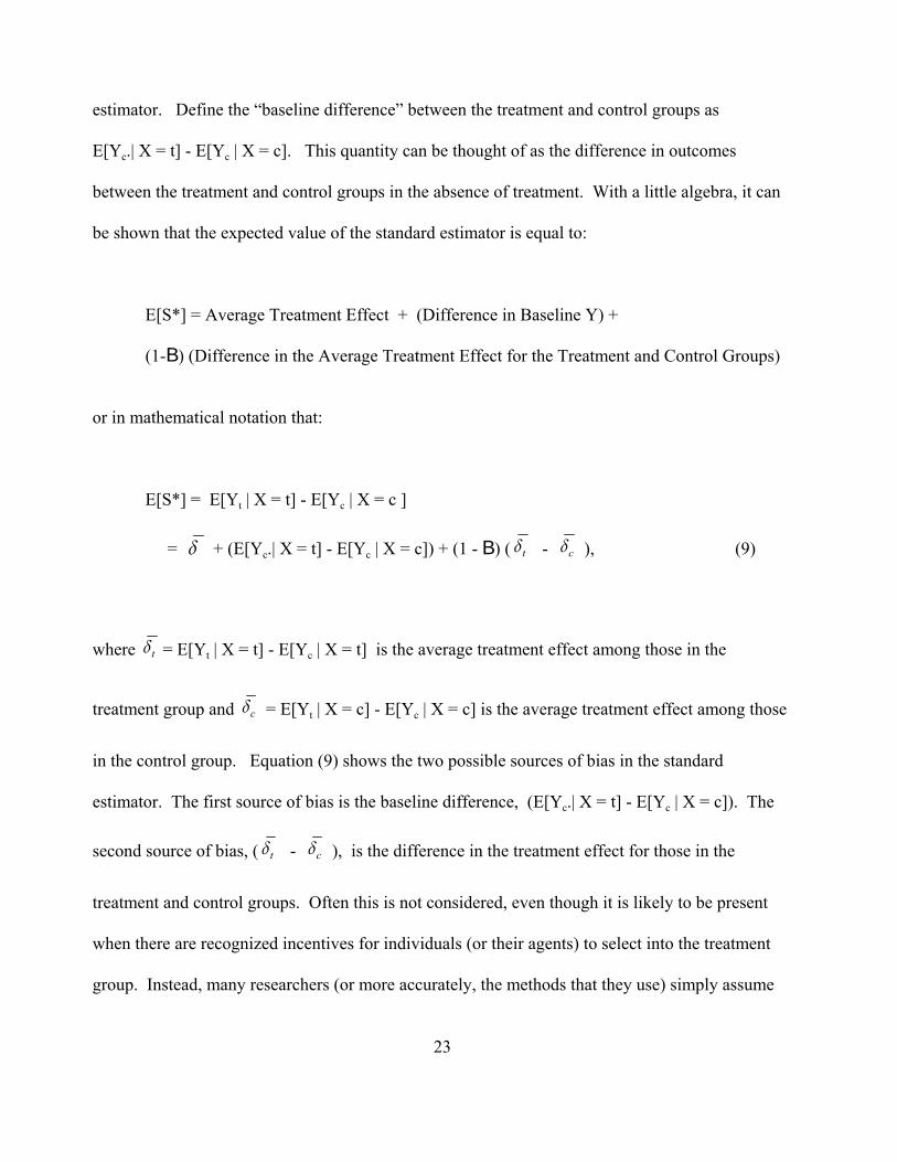
estimator. Define the “baseline difference” between the treatment and control groups as

E[Yc.| X = t] - E[Yc | X = c]. This quantity can be thought of as the difference in outcomes

between the treatment and control groups in the absence of treatment. With a little algebra, it can

be shown that the expected value of the standard estimator is equal to:

E[S*] = Average Treatment Effect + (Difference in Baseline Y) +

(1-B) (Difference in the Average Treatment Effect for the Treatment and Control Groups)

or in mathematical notation that:

E[S*] = E[Yt | X = t] - E[Yc | X = c ]

= + (E[Yc.| X = t] - E[Yc | X = c]) + (1 - B) ( - ), (9)δ δ t δc

where = E[Yt | X = t] - E[Yc | X = t] is the average treatment effect among those in theδ t

treatment group and = E[Yt | X = c] - E[Yc | X = c] is the average treatment effect among thoseδc

in the control group. Equation (9) shows the two possible sources of bias in the standard

estimator. The first source of bias is the baseline difference, (E[Yc.| X = t] - E[Yc | X = c]). The

second source of bias, ( - ), is the difference in the treatment effect for those in theδ t δc

treatment and control groups. Often this is not considered, even though it is likely to be present

when there are recognized incentives for individuals (or their agents) to select into the treatment

group. Instead, many researchers (or more accurately, the methods that they use) simply assume

24

that the treatment effect is constant in the population, even when commonsense dictates that the

assumption is clearly implausible (Heckman 1997a, 1997b; Heckman, Smith, and Clements 1997;

Heckman and Robb 1985, 1986, 1988).

To clarify these issues consider a specific example—the effects of a job training program

on individuals’ later earnings. Assume that potential trainees consist of both unskilled and skilled

workers. Further assume that the training program is aimed at upgrading the skills of unskilled

workers who are in fact the individuals who take the program. Plausibly, in the absence of the

training program, the earnings of unskilled workers would be lower on average than those of the

skilled workers. Thus a simple comparison of the post training earnings of the unskilled workers

to those of the skilled workers would understate the effect of the program because it fails to adjust

for these preprogram differences. However, it might well be the case that the training program

raises the earnings of unskilled workers, but would have no effect on the earnings of skilled

workers. In this case, net of the preprogram differences in earnings, the difference in the post-

training earnings of unskilled workers and those of skilled workers would overstate the average

effect of training for the two groups as a whole.

Note, however, that in this example the average treatment effect over the combined two

groups, , is unlikely to be the quantity of interest. In particular, what is likely to be of interest isδ

whether the unskilled workers have benefitted from the program. Heckman (1992, 1996, 1997a)

and Heckman, Smith, and Clements (1997) have argued that in a variety of policy contexts, it is

the average treatment effect for the treated that is of substantive interest. The essence of their

argument is that in deciding whether a policy is beneficial, our interest is not whether on average

the program is beneficial for all individuals, but rather whether it is beneficial for those individuals

25

who would be either assigned or who would assign themselves to the treatment. Fortunately, this

situation is salutatory from a statistical perspective since most methods of adjustment only attempt

elimination of the baseline difference. Few techniques are available to adjust for the differential

treatment effects component of the bias. Often with non-experimental data the best that we can do

is to estimate the effect of treatment on the treated.

Randomized Experiments. Since Fisher invented the concept of randomization,

experimenters in many disciplines have argued that in a randomized experiment inferences about

the effect of X could be made using the standard estimator. It is important to note that although

statisticians had used Neyman’s notation to make this argument, outside of statistics where this

notation was not well known, the argument was sustained largely by intuition, without explicit

consideration of the estimand (6).

To intuitively understand how randomization works, note that in a randomized experiment,

the units for whom X = t and the units for whom X = c are each random samples from the

population of interest. Hence, is an unbiased and consistent estimate of E(Yt) and is anYt Yc

unbiased and consistent estimate of E(Yc) . As a result:

E[ - ] = E[ ] - E[ ] = E[Yt]- E[Yc] = E [Yt - Yc] = (10)Yt Yc Yt Yt δ

Of course, in practice randomized studies have their difficulties as well. Not all subjects will

comply with their treatment protocol. Treatment effects may be different for compilers and non-

compilers. Some statisticians argue that the effect of interest in this case is , while others argueδ

26

that the estimate of interest is the average causal effect in the sub-population of compilers. (We

discuss the technical aspects of this issue further in the section below on instrumental variables.

Also see Angrist, Imbens, and Rubin (1996)). Experimental mortality is another well known threat

to inference (Campbell and Stanley 1966). The usual approach to this problem is to assume that

the only impact of experimental mortality is to reduce the size of the experimental groups, thereby

increasing the standard errors of estimates. This is tantamount to assuming that experimental

mortality is independent of the potential responses Yt and Yc .

Ignorability. Sociologists do not typically conduct randomized studies. It might appear

that the foregoing results suggest that it is not possible to make well supported causal inferences

from observational studies. This is incorrect. Random assignment is sufficient (but not necessary)

for E(Yt ) = E(Yt | X = t) and E(Yc) = E(Yc | X = c), (which is necessary for the difference between

the sample means to be an unbiased and consistent estimator of (1), the average causal effect).

A more general sufficient condition for the standard estimator to be unbiased and

consistent is what is known as ignorability. Ignorability holds if:

(Yt , Yc ) z X , (11)

where “ z” indicates that Yx and X are independent, that is, Yt and Yc are independent of X.2

Note that ignorability does not imply that X and the observed Y are independent. In fact, in many

situations they will be related either because there is a treatment effect and/or systematic

differences in who is assigned to the treatment and control group. Ignorability is a more general

condition than random assignment, since random assignment insures that treatment assignment, Xi,

27

is independent of all variables whereas ignorability only requires that the potential outcomes, Yx,

be independent of Xi.

To understand why ignorability is sufficient for consistency of the standard estimator,

consider the well known theorem from probability theory that if two random variables (or

vectors), Z and W are independent ( Z z W), then the mean of Z conditional on W is equal to the

conditional mean of Z, that is, E(Z | W) = E(Z). Thus a sufficient condition that E(Yx ) = E(Yx | X

= x) is for Yx z X for x = t, c. In other words, the potential responses Yt and Yc are independent

of X, the treatment assignment.

Now consider the case where interest focuses on causal analysis within subgroups. The

sample data can be used to estimate E(Yt | X = 0, Z =z) and E(Yc | X =1, Z = z), respectively. In

the case where Z takes on a small number of values, the sample means within subgroups (provided

there are cases in the data) can be used to estimate these quantities. Here Yt and Yc need to be

independent of X within the strata defined by the different levels of Z. Arguing as before, when X

= x, the response Y that is observed is Yx; thus E[Y | X =x, Z =z] = E[Yx, | X = x, Z = z]. In order

that E[Yx | X = x, Z = z] = E[ Yx | Z =z], it is sufficient that:

(Yt, Yc ) z X | Z = z . (12)

That is, treatment assignment must be ignorable within the strata defined by Z. When this holds,

it implies that:

E[Yt | X = t, Z =z] - E[Yc | X = c, Z = z] = E[Yt | Z =z) - E(Yc | Z = z] = , (13)δ z

28

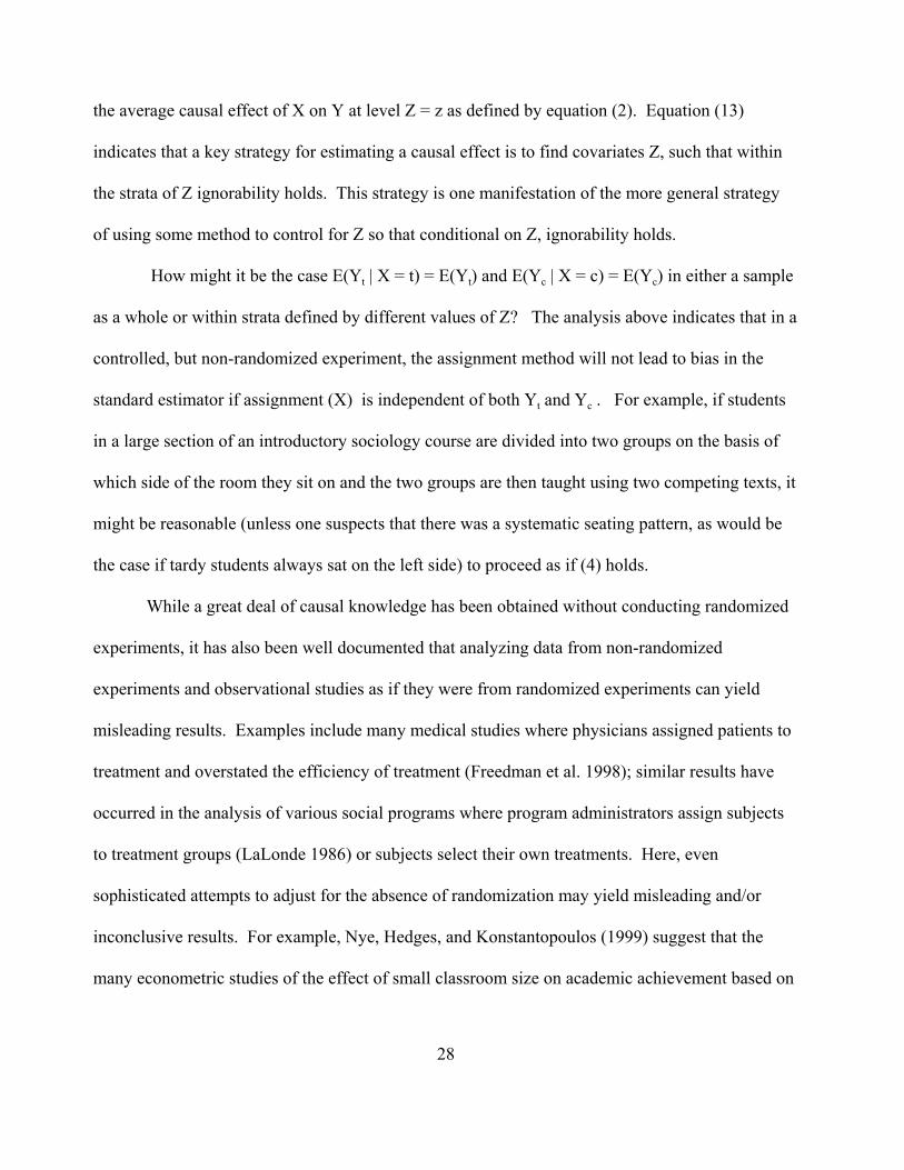
the average causal effect of X on Y at level Z = z as defined by equation (2). Equation (13)

indicates that a key strategy for estimating a causal effect is to find covariates Z, such that within

the strata of Z ignorability holds. This strategy is one manifestation of the more general strategy

of using some method to control for Z so that conditional on Z, ignorability holds.

How might it be the case E(Yt | X = t) = E(Yt) and E(Yc | X = c) = E(Yc) in either a sample

as a whole or within strata defined by different values of Z? The analysis above indicates that in a

controlled, but non-randomized experiment, the assignment method will not lead to bias in the

standard estimator if assignment (X) is independent of both Yt and Yc . For example, if students

in a large section of an introductory sociology course are divided into two groups on the basis of

which side of the room they sit on and the two groups are then taught using two competing texts, it

might be reasonable (unless one suspects that there was a systematic seating pattern, as would be

the case if tardy students always sat on the left side) to proceed as if (4) holds.

While a great deal of causal knowledge has been obtained without conducting randomized

experiments, it has also been well documented that analyzing data from non-randomized

experiments and observational studies as if they were from randomized experiments can yield

misleading results. Examples include many medical studies where physicians assigned patients to

treatment and overstated the efficiency of treatment (Freedman et al. 1998); similar results have

occurred in the analysis of various social programs where program administrators assign subjects

to treatment groups (LaLonde 1986) or subjects select their own treatments. Here, even

sophisticated attempts to adjust for the absence of randomization may yield misleading and/or

inconclusive results. For example, Nye, Hedges, and Konstantopoulos (1999) suggest that the

many econometric studies of the effect of small classroom size on academic achievement based on

29

observational studies and non-randomized experiments have not yielded a set of consistent

conclusions, much less good estimates of the true effects. By way of contrast, these authors

demonstrate that there are long-term beneficial effects of small classroom size using data from a

large randomized experiment – Project Star.

Propensity Scores and the Assignment Equation. If we have a large sample and there is

good reason to believe that the Yx and X are independent within the strata that are defined by

some set of variables Z, then our analysis task is conceptually straightforward. We can simply use

the standard estimator to estimate average causal effects within strata. If an estimate of the

average effect for the population as a whole is desired, strata level average effects can be

combined by using a weighted average, where the weights are proportionate to the population

proportions within each strata.

With small samples it can be either impossible or undesirable to carry out analysis within

strata. What then are we to do? Suppose that treatment assignment is not random but that the

probabilities of assignment to the treatment groups (X) are a known function of measured variables

Z (e.g. age, sex, education), that is:

Prob(X = t | Z =z ) = P(Z). (14)

Equation (14) is what is known as the assignment equation and P(Z) is what is known at the

propensity score. The propensity score is simply the probability that a unit with characteristics Z

is assigned to the treatment condition. In practice P(Z) might have the form of a logit equation. If

ignorability conditional on Z holds, then:

30

Pr( X = t | Z = z, Yt, Yc ) = Pr(X = t | Z =z). (15)

The condition expressed by equation (15) is some times known as “selection on the

observables.”(Heckman and Robb 1985). Here the probability of being assigned to the treatment

condition is a function of the observable variables Z and is conditionally independent of the (only

partially observable) variables Yt and Yc. Rosenbaum and Rubin (1983) show that under these

conditions that:

(Yt, Yc) z X | P(Z), (16)

that is, ignorability holds conditional on P(Z), the propensity score.

Equations (15) and (16) provide a critical insight. They show that what is critical in

estimating the causal effect of X is that we condition on those variables that determine assignment,

that is, Xi . This is quite different from the standard view in sociology where it is typically

thought that what is important is to take into account all the variables that are causes of Y. What

the counterfactual approach demonstrates is that what is critical is to condition on those Z’s that

result in ignorability holding, that is Yt and Yc being independent of X.

Rosenbaum and Rubin (1983) show that over repeated samples there is nothing to be

gained by stratifying in a more refined way on the variables in Z beyond the strata defined by

propensity score. The propensity score contains all the information that is needed to create what is

known as a balanced design – i.e. a design where the treatment and control groups have identical

31

distributions on the covariates.

If our sample is sufficiently large so that it is possible to stratify on the propensity score,

P(Z), then as before we can use the standard estimator within strata defined by P(Z). If this is not

the case, the propensity score can still be a key ingredient in an analysis. We discuss this in the

next section, where we examine matching estimators.

In general the propensity score is not known. Typically, it is estimated using a logit

model. One, however, cannot actually know that a particular Z includes all the relevant variables;

thus, biases arising from unmeasured variables may be present. Detecting such biases and

assessing the uncertainty due to potential biases is important; such issues have received a great

deal of attention in the work of Rosenbaum (for a summary, see chapters 4-6 of Rosenbaum

(1995)).

V. Estimation of Causal Effects

For many readers the discussion to this point may bear little relation to what they learned in

statistics courses as graduate students. As noted at the beginning of this chapter, a principal virtue

of the counterfactual model is that it provides a framework within which to assess whether

estimators from various statistical models can appropriately be interpreted as estimating causal

effects.

In this final section of the paper, we want to briefly examine the properties of a few

statistical methods when they are considered from the perspective of the counterfactual model. In

particular, we will examine matching, regression, instrumental variables, and methods for

32

longitudinal data. Space limitations prevent us from considering these methods in any depth.

However, other chapters in this handbook provide comprehensive introductions to many of these

methods.

Matching. Matching is commonly used in biomedical research. It is closely related to

stratification. In essence matching is equivalent to stratification where each strata has only two

elements, with one element assigned to the control condition and the other to the treatment. Smith

(1997) provides an excellent introduction for sociologists. To match, one identifies individuals in

the treatment and control groups with equivalent or at least similar values of the covariates Z and

matches them, creating a new sample of matched cases. The standard estimator is then applied to

the matched sample. By construction, the treatment and control cases in the matched sample have

identical values of Z (or nearly so). Thus, matching eliminates the effect of any potential

differences in the distribution of Z between the treatment and control groups by equating the

distribution of Z across the two groups.

Matching has several advantages. First, it makes no assumption about the functional form

of the dependence between the outcome of interest and Z’s. As such, it is a type of nonparametric

estimator. Second, matching insures that the Z’s in the treatment group are similar (matched) to

those in the control group.3 Thus, matching prevents us from comparing units in the treatment and

control groups that are dissimilar. We do not compare “apples” and “oranges”. Third, since fewer

parameters are estimated than in a regression model, matching may be more efficient. Efficiency

can be important with small samples.

A major problem with the traditional matching approach, however, is that if there are more

33

than a few covariates in Z, it may be difficult to find both treatment and control cases that match

unless an enormous sample of data is available. Matching on the propensity score is an attractive

alternative to attempting to match across all covariates in Z since it involves matching on only a

single dimension. Nearest available matching on the estimated propensity score is the most

common and one of the simplest methods (see Rosenbaum and Rubin 1985). First, the propensity

scores for all individuals are estimated with a standard logit or probit model. Individuals in the

treatment group are then listed in random order.4 The first treatment case is selected, and its

propensity score is noted. The case is then matched to the control case with the closest propensity

score. Both cases are then removed from their respective lists, the second treatment case is

matched to the remaining control case with the closest propensity score. This procedure is

repeated until all the treatment cases are matched. Other matching techniques that use propensity

scores are implemented by: (1) using different methods and different sets of covariates to estimate

propensity scores, (2) matching on key covariates in Z that one wants to guarantee balance on first

and then matching on propensity scores, (3) defining the closeness of propensity scores and Z’s in

different ways, and/or (4) matching multiple control cases to each treatment case (see Rosenbaum

1995; Rubin and Thomas 1996; Smith 1997).

Matching works because it amounts to conditioning on the propensity score. Thus if

ignorability holds conditional on the propensity score, the standard estimator on the matched

sample will be unbiased and consistent. A couple of caveats, however, are in order about

matching. First, if there are treatment cases where there are no matches, the estimated average

causal effect only applies to cases of the sample of treated cases for which there are matches.

34

Second, the consistency of the standard estimator on the matched sample under ignorability holds

only if cases are truly matched on a random basis. Often for a particular treatment case there may

be only one (or perhaps a couple) of control cases that are an appropriate match. In this case, the

matching process is clearly not random. As a result, although the original sample may be balanced

conditional on the propensity score, this may not be true of the matched sample that has been

derived from the overall sample. Because of this, it is good practice to examine the means and

variances of the covariates in Z’s in the treatment and control groups in the matched samples to

insure that they are comparable. If one believes that one’s outcomes are likely to be a function of

higher order nonlinear terms or interactions of the covariates, then the two groups must be similar

on these moments of Z also.5

An alternative approach that avoids the latter problem with matching is to use the original

sample of treatment and control cases, but to weight cases by the inverse of their propensity

scores. As with matching, this creates a balanced sample. One then computes the standard

estimator on the weighted sample. As in the case with matching, this is a form of non-parametric

estimation. Thus, if ignorability holds, the standard estimator will provide an unbiased and

consistent estimate of the average causal effect. In general, however, one should probably exclude

treatment and control cases that do not have counterparts with similar propensity scores (Robbins

2000). One wants to avoid the problem of comparing “apples” to “oranges”. This means that one

should first omit from the sample those treatment and control cases that do not have similar

counterparts in the other group and then re-estimate the remaining cases’ propensity scores. This

re-estimated propensity score can then be used in an analysis of the inverse weighted sample. A

35

second advantage of this estimator is that it will generally use most of the sample, whereas

matching can involve throwing out a considerable number of cases. As far as we are aware, little

work has been done that investigates this estimator.6

Regression. Regression models (and various extensions thereof, such as logistic

regression) are frequently used by quantitative social scientists. Typically, such models are

parametric, specifying the functional form of the relationship between independent variables and

the response. If the model is correctly specified, matching, which provides a non-parametric

estimator, is inefficient relative to modeling, as observations are discarded. However, if this is not

the case, inconsistent estimates of effects will result when such models are used.

As noted above, it is standard to interpret the coefficient for a particular variable in a

regression model as representing the causal effect of that variable on the outcome “holding all

other variables in the model constant.” We hope by this point that we have convinced the reader

that this interpretation is almost always unreasonable. The inferential task is difficult enough

when there is only a single variable X whose causal effect is of interest. We view the all too

common attempt when one has non-experimental data to make causal inferences about a series of

X’s within a single model as hazardous. The threats to the validity of such claims are simply too

great in most circumstances to make such inferences plausible. The relevant question, then, is

under what conditions in the context of the counterfactual model can a regression estimate for a

single variable be interpreted as a causal effect?

Above we have treated Xi as a dichotomous variable taking on values “t” and “c”. More

generally, we may let Xi be a numerical valued variable taking on many values; as before, Xi is

36

the observed (or factual) level of the treatment. Consider the following standard regression

equation:

Yi = $0 + Xi $ + , i , (17)

where ,i = Yi - ($0 + Xi $ ), $ = Cov(Y,X)/Var (X), and $0 = , the standard ordinaryY - Xβ

least squares estimators. Note that this equation only pertains to the one value of Yi and Xi that is

observed for each individual in the data. This equation could be augmented to include a matrix of

control variables Z. If ,i is assumed to be independent of Xi , (17) implies: 7

E[Y | X] = $0 + Xi $. (18)

Now consider the following equation as part of a counterfactual model:

Yxi = ( + Xi + exi . (19)δ

Here Yxi has a distinct value for every value of Xi, , factual and counterfactual. In equation (19),

represents the average causal effect of Xi on Yxi.. The critical question is under whatδ

conditions does $ = , that is, does estimation of $ provide an estimate of the average causalδ

37

effect of Xi, ?δ

As in the case of the standard estimator, a sufficient condition is the Yxi and Xi (the realized

Xi) be independent of each other, that is, ignorability holds. This condition is equivalent to each of

the exi and Xi being independent. Note, however, that this is not equivalent to the condition that ,i

and Xi be independent, a condition that is sufficient for OLS to consistently estimate the

conditional expectation equation (18). The error, ,i, is associated with the realized values of Yxi,

Yi , and consists of a single value for each individual, i, whereas exi is a vector of values for each i,

with one value for each potential value of Xi and its value Yxi. In general, the independence of Xi

and ,i does not imply ignorability. This is critical. Equation (18) provides a description of the

data – how the expected value of Y varies with X. Equation (19) defines a causal relation between

Y and X. In general these will be different.

Adopting a counterfactual perspective has important implications for how one does

regression analysis. The standard approach in regression analysis is to determine the set of

variables needed to predict a dependent variable Y. Typically, the researcher enters variables into

a regression equation and uses t-tests and F-tests to determine whether the inclusion of a variable

or set of variables significantly increases R2.

From a counterfactual perspective the ability to predict Y and thus the standard t and F

tests are irrelevant. Rather the focus, at least in the simplest cases, is on the estimation of the

causal effect of a single variable (what we have called the treatment effect). The key question is

whether the regression equation includes the appropriate set of covariates such that ignorability

holds (Pratt and Schlaifer 1988). To attempt to achieve this, the researcher needs to stratify on, or

38

enter as controls, variables that determine the treatment variable, Xi. These variables may or may

not be significantly related to the dependent variable Yi. The criteria for deciding whether a

variable should be included in the equation is not whether it is significant or not, but rather

whether our estimate of the treatment effect and the confidence interval surrounding it is changed

by the variable’s inclusion. In particular, we need to include variables that are likely to be highly

correlated with Xi since their inclusion is likely to change the inferences we make about the likely

size of X’s effect even though these variables may well not significantly increase R2 precisely

because they are highly correlated with X. Strong candidates for controls in the regression

equation are variables that the researcher believes are likely to determine X. In the particular case

where X is dichotomous we can borrow the strategy used in matching and condition on the

propensity score by entering it as a control variable. This approach may be particularly attractive

when there are few degrees of freedom associated with the regression model.

Instrumental Variables. The counterfactual framework has provided important insight into

instrumental variable estimators (Winship and Morgan 1999). The typical assumption in

instrumental variables is that the effect of treatment is constant across the populations. In many

situations, however, this is unreasonable. What does an instrumental variable estimator estimate

when the treatment effects vary? Recent work by Imbens and Angrist (1994), Angrist and

Imbens (1995), Angrist, Imbens, and Rubin (1996), and Imbens and Rubin (1997) investigates this

issue by extending the potential outcome framework discussed at the beginning of this paper. This

extension is accomplished by assuming that treatment received is a function of an exogenous

instrument Ri . Ri might be the treatment individuals are assigned to (Angrist et al. 1996), an

39

incentive to be in either the treatment or control group, or any variable that directly affects the

treatment received, but not the treatment outcome.

For simplicity, assume that both the treatment and the instrument are binary. Treatment is

determined nonrandomly. However, an incentive to enroll in the treatment program (e.g., a cash

subsidy), Ri, is assigned randomly. Ri is an instrument for Xi in that Ri affects Xi., but has no direct

effect on Yi . When both the treatment and incentive are binary, individuals eligible to receive the

treatment can be divided into four mutually exclusive groups termed “compliers”, “defiers”,

“always takers” and “never takers”. Individuals who would enroll in the program if offered the

incentive and who would not enroll in the program if not offered the incentive are labeled

“compliers” (i.e., when Ri = 1, Xi = t and when Ri = 0, Xi = c ). Likewise, individuals who would

only enroll in the program if not offered the incentive are “defiers” (i.e.,when Ri = 1, Xi = c and

when Ri = 0, Xi = t). Individuals who would always enroll in the program, regardless of the

incentive, are “always-takers” (i.e.,when Ri = 1, Xi = t and when Ri = 0, Xi = t). Finally,

individuals who would never enroll in the program, regardless of the incentive, are “never-takers”

(i.e.,when Ri = 1, Xi = c and when Ri = 0, Xi = c). Note that the usage here is nonstandard in that

the terms “compliers” and “defiers” refer to how an individual responds to the incentive, not

simply whether they comply or not with their treatment assignment in a traditional experiment, the

standard denotation of these terms.

Based on the potential treatment assignment function, Imbens and Angrist (1994) define a

monotonicity condition. For all individuals, an increase in the incentive, Ri, must either leave their

treatment status the same, or among individuals who change, cause them to switch in the same

40

direction. For example, the typical case would be that an increase in the incentive would cause

more individuals to adopt the treatment condition, but would not result in anyone refusing the

treatment condition who had previously accepted it. The general assumption is that there be either

defiers or compliers but not both in the population.8

When the treatment assignment process satisfies the monotonicity condition, the

conventional IV estimate is an estimate of what is defined as the local average treatment effect

(LATE), the average treatment effect for either compliers alone or for defiers alone, depending on

which group exists in the population.9 LATE is the average effect for that subset of the population

whose treatment status is changed by the instrument, that is, that set of individuals whose

treatment status can be potentially manipulated by the instrument. The individual-level treatment

effects of always-takers and never-takers are not included in LATE.

Because of LATE’s nature, it has three problems: (1) LATE is determined by the

instrument and thus different instruments will give different average treatment effects; (2) LATE is

the average treatment effect for a subset of individuals that is unobservable; (3) LATE can

sometimes be hard to interpret when the instrument measures something other than an incentive to

which individuals respond.

Longitudinal Data. Longitudinal data is often described as a panacea for problems of

causal inference. Nothing could be farther from the truth. As in any causal analysis, the critical

issue is what assumptions the analysis makes about the counterfactual values. As discussed below,

different methods of analysis make quite different assumptions. Unfortunately, these are often not

even examined, much less tested. Here we briefly discuss these issues (see Winship and Morgan

41

(1999) who provide a more extensive discussion).

Let equal the value of the observed Y for person i at time s. Let equal the value ofYis Yti

s

Y for individual i under either the factual or counterfactual condition of receiving the treatment.

Let equal the value of the Y for individual i under either the factual or counterfactual conditionYcis

of not receiving the treatment. Let the treatment occur at a single point in time, s’. We assume

that for s < s’, = , that is the treatment has no effect on an individual’s response prior toYtis Yci

s

the treatment. Below we discuss how a test of this assumption provides an important method for

detecting model mis-specification.

A variety of methods are often used to analyze data of the above type. We discuss the two

most commonly used in sociology with the aim of demonstrating the different assumptions each

makes about the value of under the counterfactual condition. After this, we briefly discuss theYs

implications of the counterfactual perspective for the analysis of longitudinal data.

The simplest case uses individuals as their own control cases. Specifically, if we have both

test and pretest values on Y, and where s < s’ < s*, ( - ) is an estimate of theYis Yi

s* Yis* Yi

s

treatment effect for individual i. The problem with this approach is that it assumes that Y would

be constant between s and s* in the absence of treatment. Changes may occur because of aging

or changes in the environment. If one’s data contains longitudinal information for a control group,

however, the assumption of no systematic increase and decrease with time in Y in the absence of

treatment can be tested. Preferably, the control group will consist of individuals who are similar to

42

those in the treatment group both in terms of covariates Z and their initial observations on Y. This

might be accomplished, for example, using matching. The simplest approach then would be to test

whether the mean or median of Y of the control group shifts between times s and s*. This test, of

course, is only useful if we are correct in assuming that in the absence of treatment, the responses

of individuals in the treatment and control group would change with time in similar ways.

If Y does systematically change over time in the absence of treatment, what is the

researcher to do? Two very different choices are available. One could analyze the post-test

observations using cross-sectional methods such as matching or regression. Here the presence of

pretest data is a considerable advantage. Specifically, we can also analyze the pretest observations

on the treatment and control groups as if they were post-test observations using the same cross-

sectional methods (Heckman and Hotz 1989, Rosenbaum 1995). Since the treatment group has yet

to receive the treatment, a finding of a treatment effect in the pretest data is evidence that one’s

method inadequately adjusts for differences between the treatment and control groups. A

considerable advantage of having pretest and post-test data either when one is using individuals as

their own controls or using cross-sectional methods to estimate a treatment effect is that the

availability of pretest data allows the researcher to test whether the particular cross-sectional

model under consideration is consistent with the data.

The other approach when one has longitudinal data is to use the fact that one has

observations over time to adjust for possible differences between the treatment and control groups.

The two most common methods used in sociology are change score analysis and the analysis of

covariance (Allison 1990, Winship and Morgan 1999). Change score analysis amounts to

43

estimating the following regression equation:

( - ) = Xi $+ ui , (20)Yis* Yi

s

where additional covariates Z could be potentially added as controls. Alternatively, analysis of

covariance amounts to estimating the following equation:

= " + Xi $+ ui (21)Yis* Yi

s

or equivalently:

( -" ) = Xi $+ ui , (22)Yis* Yi

s

where, as before, covariates Z could be added to the equation as controls. As we discuss below, "

will always be between zero and one. Comparing equations (20) and (21) we see that both

methods involve adjusting the post-test outcome, by subtracting out some portion of the pretestYis*

outcome, . Change score analysis amounts to setting the adjustment factor, ", to one. Yis

A large literature has debated the relative merits of these two approaches (see Allison 1990

for a discussion). From the counterfactual perspective, the key observation is that both methods

make different assumptions about how will change over time in the absence of treatment. Yis

44

Change score analysis assumes that in the absence of treatment, differences, on average, between

individuals over time will remain constant. Returning to our old convention that X = t or c, change

score analysis implies that:

E[ | X = t ] - E[ | X = c] = E[ | X = t ] - E[ | X = c ], (23)Ycis Yci

s Ycis* Yci

s*

that is, the difference in the mean of Yc for individuals in the treatment group and individuals in

the control group will remain constant between times s and s*. Alternatively, the analysis of

covariance model assumes that:

E[ | X = t ] - E[ | X = c] = " (E[ | X = t ] - E[ | X = c ]), (24)Ycis Yci

s Ycis* Yci

s*

that is, the difference between the mean of Yc for individuals in the treatment group and those in

the control group will shrink by a factor ".

It is often argued that a distinct advantage of the analysis of covariance model over the

change score model is that the adjustment factor, ", is estimated. This is incorrect if equation (20)

is estimated by OLS, which is the standard procedure.10 In this case, ", by construction, will be

equal to the intragroup correlation between and . As a result, " will be between zero andYis* Yi

s

one, except in rare cases where it is negative.

Comparing equations (22) and (23) shows that change score analysis and analysis of

45

covariance models make different assumptions about how the difference between E[ ] for theYcis

treatment and control groups change with time. Change score analysis assumes that this difference

will remain constant, whereas the analysis of covariance assumes that it will shrink by a fixed

factor ", the within group correlation between the responses between time s and s*. Whether $ in

equation ( 20) or equation (21) consistently estimates will depend on which, if either, of theseδ

assumptions is correct (Holland and Rubin 1983).

As Heckman and Hotz (1989) have argued, with only a single pretest and post-test, it is

impossible to determine which assumption is correct since there are not observations at a sufficient

number of time points to determine how the difference in average outcome for the treatment and

control groups changes over time in the absence of treatment. In fact, the assumptions in the

change score and analysis of covariance model may be simultaneously incorrect. The difference

between the outcomes for the treatment and control groups may shrink by a factor other than ", or

the difference might potentially increase which would be inconsistent with both models. A

possible example of the latter would be in the examination of the effects of educational attainment

on mental ability of children (Winship and Korenman 1998). A plausible assumption in this case

is that in the absence of additional education, the difference in mental ability between higher and

lower ability children would grow with age.

Other more sophisticated methods for analyzing longitudinal data are available.

Economists are particularly interested in what is known as the difference in difference model (e.g

Card and Krueger 1995, Ashenfelter and Card 1985). This model is similar to the change score

46

model except instead of assuming that in the absence of treatment the difference between

individuals outcomes remains constant, it assumes that this difference changes at a fixed linear

rate. The change score model allows the intercept to vary across individuals. The difference in

difference model in addition allows the coefficient on time/age to vary across individuals.

Heckman and Robb (1986, 1988) provide an extensive review of different methods.

Different methods make different assumptions about what will occur in the absence of

treatment, that is they make different assumptions about what will be true in the counterfactual

condition. As a result, different methods are likely to provide different estimates of the treatment

effect (LaLonde 1986). Which method should a researcher use? In some cases, theoretical

considerations may suggest that one method is more appropriate than another (Allison 1990). In

sociology, however, our theories are often sufficiently weak or there may be competing theories

such that it is impossible with any confidence to assume that one model as opposed to the others is

the appropriate model for analysis.

Heckman and Hotz (1989) argue that it is critical that one have sufficient pretest (or post-

test) observations so that it is possible to test one’s model against the data. As discussed earlier,

one can treat one’s pretest data as if it, or some portion of it, is post-test data and then estimate

whether there is evidence of a “treatment” effect on this data. One can also perform a similar

analysis when one has multiple post-test values dividing them into a “pretest” and “post-test”

group. Lack of evidence for a treatment effect is evidence that the model being used has

appropriately adjusted for differences between the treatment and control groups. Of course, more

than one model may be consistent with the data and these different models may produce different

47

estimates of the treatment effect. Unless there is a compelling reason to choose one model over

another, one should pool one’s estimates of the effect across models. Raftery (1995) discusses

how this can be done within a Bayesian framework.

Conclusion

The purpose of this chapter has been to provide an introduction to the counterfactual model

of causal inference and to briefly examine its implications for the statistical analysis of causal

effects. In the introduction we argued that the counterfactual model of causal inference (hereafter

CMCI) had the potential to change the way that sociologists carried out empirical analyses. We

summarize the chapter by providing a list of what we believe are the most important contributions

and insights of CMCI for empirical research:

1. Estimating the effect of a single variable (treatment) on an outcome is quite difficult.Attempts to estimate the effects of multiple variables simultaneously are generally ill-advised.

2. CMCI provides a general framework for evaluating the conditions under which specificestimators can be interpreted as estimating a causal effect.

3. A particular strength of CMCI is its ability to make explicit the possibility that thesize of a treatment effect may vary across individuals.

4. Often it is only possible to estimate the size of the treatment effect for the treated.However, under some circumstances this is precisely what is of interest.

5. Causal analysis is at its core a missing data problem. The key question is what the valuesof the outcome would have been under the counterfactual condition.

6. Different assumptions about the counterfactual values will typically result in differentestimates of the causal effect.

48

7. CMCI asks the researcher to fully specify the implicit manipulation or “experiment” associated with the estimation of a causal effect. In some cases, such as when estimatingthe effect of gender, what the manipulation of interest is may be unclear.

8. An effect may be inconsistently estimated for two different reasons: (1) failure to controlfor differences between the treatment and control group in the absence of treatment; (2) failure to take account of the fact that the size of the treatment effect differs for individualsin the treatment and control groups.

9. In order to consistently estimate a causal effect, ignorability (or ignorability givencovariates) must hold, i.e. treatment received (X) must be independent of the partiallyobserved outcome variables Yx.

10. The key to consistently estimating a causal effect is to control for those variables, eitherby matching, stratification, or regression, that determine (or are associated with) treatmentstatus.

11. Matching provides a powerful nonparametric alternative to regression for theestimation

of a causal effect that should be more frequently used by sociologists.

12. The traditional logic in which a variable or variables are included in a regression modelbecause they significantly increase R2 as judged by a t-test or F-test are irrelevant to theassessment of the causal effect of a particular variable (the treatment).

13. Variables should be included as controls if they substantially change the estimateof the treatment effect. Often these will be variables that are highly correlated withthe treatment variable and as such may have insignificant coefficients.

14. Instrumental variable estimators only estimate the effect of the treatment for thoseindividuals whose treatment status is changed by varying the value of the instrument. Ingeneral, it is impossible to identify who belongs to this group.

15. Longitudinal data is not a panacea for causal analysis. As with any causal analysis,assumptions need to be made about the values of the outcome under the counterfactualcondition. Different models involve different assumptions and as a result will generallygive different estimates.

16. With longitudinal data, as with any analysis, it is important to test whether theassumptions implicit in the model hold by testing the model against the data.

49

The length of this list indicates that the implications for empirical research of the CMCI are

considerable. We believe that as sociologists come to better understand and appreciate the

counterfactual model, CMCI will change the way they do research. Hopefully, the consequence of

this will be much clearer thinking about causality and the problems in estimating specific causal

effects, resulting in better estimates of the size of actual effects.

REFERENCES

Allison PD. 1990. “Change Scores as Dependent Variables in Regression Analysis,” Sociological

Methodology 1990, Vol. 20, CC Clogg, ed.: 93-114.

Alwin, Duane F., and Robert M. Hauser. 1975. "The Decomposition of Effects in Path Analysis,"

American Sociological Review 40:37-47.

Anderson, John. 1938. "The Problem of Causality," Australasian Journal of Psychology and

Philosophy 16:127-142.

Angrist JD, Imbens GW. 1995. “Two-stage least squares estimation of average causal effects in

models with variable treatment intensity,” Journal of the American Statistical Association 90:431-42.

Angrist, J.D., G.W. Imbens, and D.B. Rubin. 1996. “Identification of Causal Effects Using

Instrumental Variables,” Journal of the American Statistical Association 91:444-72.

Ashenfelter, O., D. Card. 1985. “Using the Longitudinal Structure of Earnings to Estimate the

Effect of Training Programs,” The Review of Economics and Statistics 67:648-60.

Bunge, Mario A. 1979. Causality and Modern Science. (3rd ed.), New York: Dover.

Cambpell, Donald T. and J. C. Stanley. 1966. Experimental and quasi-experimental designs for

research. Chicago: Rand McNally.

Card, David, and Allan Krueger. 1995. Myth and measurement : the new economics of the minimum

wage. Princeton, N.J. : Princeton University Press.

Collingwood, Robin. G. (1940) 1948. An Essay on Metaphysics. Oxford: Oxford University Press.

Cox, David R. 1958. The Planning of Experiments. New York: John Wiley.

Davis, Joyce. 2000. "PubNet: A Case Study of Race, Gender, and Nationality in a Virtual

Organization." Unpublished. Department of Sociology, Harvard University.

Ducasse, Curt J. (1926) 1975. "On the Nature and Observability of the Causal Relation". Pp. 114-

125 in Causation and Conditionals, Ernest Sosa (ed.) London: Oxford University Press.

Duncan, Otis D. 1966. "Path Analysis: Sociological Examples," American Journal of Sociology 72:1-

16.

Ferguson, Niall. 1997. "Virtual History: Towards a `Chaotic' Theory of the Past." Pp. 1-90 in

Virtual History: Alternatives and Counterfactuals, Niall Ferguson (ed.). London: Picador.

Freedman, David, Robert Pisani, and Roger Purves. 1998. Statistics (3rd editor). New York: W.W.

Norton.

Geweke, John. 1984. "Inference and Causality in Economic Time Series Models". Pp. 1101-1144

in Handbook of Econometrics (Vol. 2), Zvi Griliches and Michael E. Intriligator (eds.). Amsterdam:

North Holland.

Goldin, Claudia. 1999. “Orchestrating Impartiality: The Impact of “Blind” Auditions on Female

Musicians.” Unpublished. Department of Economics, Harvard University.

Granger, Clive W. 1969. "Investigating Causal Relationships by Econometric Models and Cross-

Spectral Methods," Econometrica 37:424-438.

Gustafsson, Bjorn, and Mats Johansson. 1999. "What Makes Income Inequality Vary across

Countries?" American Sociological Review 64:585-685.

Harre!, Rom. 1972. The Philosophies of Science. Oxford: Oxford University Press.

Harre!, Rorn, and Edward H. Madden. 1975. Causal Powers: A Theory of Natural Necessity.

Oxford: Basil Blackwell.

Heckman, .J.J. 1978. “Dummy Endogenous Variables in a Simultaneous Equation System,”

Econometrica 46: 931-961.

Heckman, .JJ. 1992. “Randomization and Social Policy Evaluation,” Pp. 201-30 in Evaluating

Welfare and Training Programs, C.F. Manski and I. Garfinkel (eds.). Cambridge: Harvard

University Press.

Heckman, J.J. 1996. “Randomization as an Instrumental Variable,” The Review of Economics

and Statistics. 77:336-41.

Heckman, J.J. 1997a. “Instrumental Variables: A Study of Implicit Behavioral Assumptions

Used in Making Program Evaluations,” The Journal of Human Resources 32:441-62.

Heckman, J.J. 1997b. “Identifying and Estimating Counterfactuals in the Social Sciences: the

Role Rational Choice Theory.” Unpublished. The University of Chicago.

Heckman, J.J, and V.J. Hotz. 1989. “Choosing among Alternative Nonexperimental Methods

for Estimating the Impact of Social Programs: the Case of Manpower Training,” Journal of the

American Statistical Association 84:862-80.

Heckman, J.J., H. Ichimura, J. Smith, and P.Todd. 1998. “Characterizing Selection Bias Using

Experimental Data,” Econometrica 6:1017-1099.

Heckman, J. J., and R. Robb. 1985. “Alternative Methods for Evaluating the Impact of

Interventions,” Pp. 156-245 in Longitudinal analysis of labor market data, J.J. Heckman and B.

Singer (eds.). Cambridge: Cambridge University Press.

Heckman, J.J., and R. Robb. 1986. “Alternative Methods for Solving the Problem of Selection

Bias in Evaluating the Impact of Treatments on Outcomes,” Pp. 63-113 in Drawing inferences

from self-selected samples, H. Wainer (ed.). New York: Springer-Verlag.

Heckman, J.J., and R. Robb. 1988. “The Value of Longitudinal data for solving the problem of

selection bias in evaluating the impact of treatment on outcomes,” Pp. 512-38 in Panel Surveys,

G. Duncan and G. Kalton (eds). New York: Wiley.

Heckman, J.J., J. Smith, and N. Clements. 1997. “Making the Most out of Programme

Evaluations and Social Experiments: Accounting for Heterogeneity in Programme Impacts,”

Review of Economic Studies 64:487-535.

Holland, Paul W. 1986. "Statistics and Causal Inference" (with discussion), Journal of the

American Statistical Association 81:945-970.

Holland, Paul W. 1988. "Causal Inference, Path Analysis, and Recursive Structural Equation

Models" (with discussion). Pp. 449-493 in Sociological Methodology, 1988, Clifford C. Clogg

(ed.). Washington, D.C.: American Sociological Association.

Holland, Paul W., and Donald B. Rubin. 1983. "On Lord's Paradox". Pp. 3-35 in Principals of

Modern Psychological Measurement, Howard Wainer and Samuel Messick (eds.). Hillsdale, NJ:

Lawrence Erlbaum.

Imbens, G.W., and J.D. Angrist. 1994. “Identification and Estimation of Local Average

Treatment Effects. Econometrica 62:467-75 (March).

Imbens, G.W., D.B. Rubin. 1997. “Estimating Outcome Distributions for Compliers in

Instrumental Variables Models. Review of Economic Studies 64:555-574.

Joreskog, Karl G. 1977. "Structural Equation Models in the Social Sciences: Specification,

Estimation and Testing". Pp. 265-287 in Applications of Statistics, Paruchuri R. Krishnaiah (ed.)

Amsterdam: North Holland.

LaLonde, R. 1986. "Evaluating the Econometric Evaluations of Training Programs with

Experimental Data,".American Economic Review 76:604-620.

Mackie, John L. 1974. The Cement of the Universe. Oxford: Oxford University Press.

Manski CF. 1995. Identification Problems in the Social Sciences. Cambridge: Harvard

University Press.

Manski, C.F. 1997. “Monotone Treatment Response,” Econometrica 65:1311-34.

Manski, C.F., and D.S. Nagin. 1998. “Bounding Disagreements about Treatment Effects: a Case

Study of Sentencing and Recidivism,” Sociological Methodology 28:99-137.

Mill, John S. (1843) 1973. A System of Logic: Ratiocinative and Inductive, in The Collected Works

of John Stuart Mill (Vol. 7), John M. Robson (ed.). Toronto: University of Toronto Press.

Neyman, Jerzy. (1923) 1990. "On the Application of Probability Theory to Agricultural

Experiments. Essays on Principles, Section 9" (with discussion). Statistical Science 4:465-480.

Nye, Barbara, Larry V. Hedges, and Spyros Konstantopoulos. 1999. "The Long-Term Effects of

Small Classes: A Five-Year Follow-Up of the Tennessee Class Size Experiment," Educational

Evaluation and Policy Analysis 21:127-142.

Oldham, Greg R. and Benjamin I. Gordon. 1999. "Job Complexity and Employee Substance Use:

The Moderating Effects of Cognitive Ability," Journal of Health and Social Behavior 40:290-306.

Pratt, John W. and Robert Schlaifer. 1988. "On the Interpretation and Observation of Laws,”

Journal of Econometrics 39:23-52.

Pearl, Judea. 2000. Causality: Models, Reasoning, and Inference. Cambridge, England:

Cambridge University Press.

Raftery, Adrian E. 1995. “Bayesian Model Selection in Social Research,” Pp. 111-63 in

Sociological Methodology 1995, Peter V. Marsden (ed.). 111-63. Cambridge, MA.: Blackwell

Publishers.

Robins, James M. 1989. "The Analysis of Randomized and Nonrandomized AIDS Treatment

Trials Using a New Approach to Causal Inference in Longitudinal Studies," Pp. 113-159 in Health

Services Research Methodology: A Focus on AIDS, Lee Sechrest, Howard Fredman and A. Mulley

(eds.). Rockville, Md.: U.S. Department of Health and Human Services.

Robins, James M. 2000. Personal communication. June 20.

Rosenbaum, Paul R. 1984a. "From Association to Causation in Observational Studies: The Role of

Tests of Strongly Ignorable Treatment Assignment," Journal of the American Statistical Association

79:41-48.

Rosenbaum, Paul R. 1984b. "The Consequences of Adjustment for a Concomitant Variable That Has

Been Affected by the Treatment,” Journal of the Royal Statistical Society, Series A,147:656-666.

Rosenbaum, Paul R. 1986. "Dropping Out of High School in the United States: An Observational

Study," Journal of Educational Statistics 11:207-224.

Rosenbaum, Paul R. 1987. "The Role of a Second Control Group in an Observational Study" (with

discussion),” Statistical Science 2:292-316.

Rosenbaum, Paul R. 1992. "Detecting Bias with Confidence in Observational Studies," Biometrika

79:367-374.

Rosenbaum, Paul R. 1995. Observational Studies. New York: Springer-Verlag.

Rosenbaum, Paul R., and Donald B. Rubin. 1983. "The Central Role of the Propensity Score in

Observational Studies for Causal Effects," Biometrika 70:41-55.

Rosenbaum PR, Rubin DB. 1985. “Constructing a Control Group Using Multivariate Matched

Sampling Methods That Incorporate the Propensity Score,” The American Statistician 39:33-38.

Rubin, Donald B. (1974). "Estimating Causal Effects of Treatments in Randomized and

Nonrandomized Studies," Journal of Educational Psychology 66:688-701.

Rubin, Donald B. (1977). "Assignment to Treatment Groups on the Basis of a Covariate, " Journal

of Educational Statistics 2:1-26.

Rubin, Donald B. (1978). "Bayesian Inference for Causal Effects: The Role of Randomization," The

Annals of Statistics 6:34-58.

Rubin, Donald B. (1980) Comment on "Randomization Analysis of Experimental Data: The Fisher

Randomization Test," by D. Basu, Journal of the American Statistical Association 75:591-593.

Rubin, Donald B. (1990) "Formal Modes of Statistical Inference for Causal Effects," Journal of

Statistical Planning and Inference 25:279-292.

Rubin DB, Thomas N. 1996. “Matching using estimated propensity scores: Relating theory to

practice,” Biometrics 52:249-64. March.

Russell, Bertrand. 1913. "On the Notion of Cause," Proceedings of the Aristotelian Society, New

Series 13:1-26.

Simon, Herbert A. 1952. "On the Definition of the Causal Relation,” Journal of Philosophy 49:517-

528.

Smith HL. 1997. “Matching with multiple controls to estimate treatment effects in observational

studies,” Sociological Methodology 27:325-53.

Sobel, Michael E. 1990. "Effect Analysis and Causation in Linear Structural Equation Models,"

Psychometrika 55:495-515.

Sobel, Michael E. 1994. "Causal Inference in Latent Variable Models". Pp. 3-35 in Latent

Variables Analysis: Applications for Developmental Research, Alexander von Eye and Clifford C.

Clogg (eds.). Thousand Oaks, CA: Sage Publications.

Sobel, Michael E. 1995. "Causal Inference in the Social and Behavioral Sciences". Pp. 1-38 in

Handbook of Statistical Modeling for the Social and Behavioral Sciences, Gerhard Arminger,

Clifford C. Clogg and Michael E. Sobel (eds.). New York:Plenum.

Sobel, Michael E. 1998. "Causal Inference in Statistical Models of the Process of Socioeconomic

Achievement: A Case Study," Sociological Methods and Research 27:318-348.

Stark, David C., and Laszio Bruszt. 1998. Postsocialist Pathways: Transforming Politics and

Property in East Central Europe. Cambridge: Cambridge University Press.

Stinchcombe, Arthur L. 1968. Constructing Social Theories. New York: Harcourt, Brace and

World.

Winship, Christopher, and Sanders Korenman. 1997. “Does Staying in School Make You Smarter?

The Effects of Education on IQ in The Bell Curve,” Pp. 215-34 in Stephen Fienberg, Daniel

Resnick, Bernie Devlin, and Kathryn Roeder (eds.) Intelligence and Success: Is It all in the Genes:

Scientists Respond to The Bell Curve. Springer-Verlag.

Winship, Christopher, and Stephen L. Morgan. 1999. “The Estimation of Causal Effects from

Obervational Data,” The Annual Review of Sociology 25: 650-707.

1. We are grateful to Felix Elwert for bringing this example to our attention.

2. More precisely, this is the definition of strong ignorability. Weak ignorability requires that Yt and Yc be individually independent of X, whereas strong ignorability requires that they be jointlyindependent. In general, the distinction between strong and weak ignorability is of nosubstantive consequence.

3.In two empirical papers, Heckman et al. (1997, 1998) show that the bias due to selection on theunobservables, although significant and large relative to the size of the treatment effect, is smallrelative to the bias that results from having different ranges of Z’s for the treatment and controlgroups and different distributions of the Z’s across their common range. Matching solves bothof the latter problems, although the average effect is not for the total population, but only thatportion of the population where the treatment and control groups have common Z values.

4.In most empirical applications of matching techniques, the treatment group is considerablysmaller than the control group. This need not be the case in all applications, and if the reverse istrue, then the nearest available matching scheme described here runs in the opposite direction. Treatment cases would be matched to the smaller subset of control cases.

5.There is an important intellectual tension here. An attraction of the matching estimator is thatin theory it is nonparametric. This means that we do not need to know how our two outcomevariables, Yt and Yc functionally related to our Z’s. For this to actually be the case, our matcheddata set needs to be balanced on all the moments of Z. This, however, will only occur if thedistribution of Z is exactly the same for the treatment and control group. But then we are back tothe problem of traditional matching where one is trying to equate groups across a potentiallylarge number of variables.

6. In principle, the propensity score can also be entered as a control variable in a regressionmodel. Rubin and Rosenbaum have advocated matching since it implicitly deals with theproblem of nonlinearity and uses fewer degrees of freedom, making it more efficient.

7. It is only necessary the , i and Xi be mean independent, that is, E[,i | X] = 0. In general,independence is a more desirable property since it means that mean independence will holdunder any transformation of Y.

8.Note that when an instrument is valid, there must be at least some compliers or some defiers,otherwise the sample would be composed of only always-takers and never-takers. In this case, Ri would not be a valid instrument because it would have no effect on the treatment receivedand thus, Ri and treatment received would be uncorrelated.

9.The exclusion restriction that defines LATE is stronger than the conventional exclusionrestriction that the instrument must be mean-independent of the error term. Instead, Imbens andAngrist (1994) require that the instrument be fully independent of the error term. Imbens andRubin (1997) argue that the strong independence restriction is more realistic because it continues

END NOTES

to hold under transformations of the outcome variable. An assumption about the distribution ofthe outcome is thereby avoided.

10. Equation (20) could be estimated by instrumental variables. Then, however, the issues withinstrumental variable estimators discussed in the last section arise.