causal mediation analysis using r · causal mediation analysis using r ... (). ... control.valueto...
TRANSCRIPT

Causal Mediation Analysis Using R∗
Kosuke Imai† Luke Keele‡ Dustin Tingley§ Teppei Yamamoto¶
July 11, 2017
Abstract
Causal mediation analysis is widely used across many disciplines to investigate possible
causal mechanisms. Such an analysis allows researchers to explore various causal pathways,
going beyond the estimation of simple causal effects. Recently, Imai, Keele, and Yamamoto
(2010c) and Imai, Keele, and Tingley (2010b) developed general algorithms to estimate causal
mediation effects with the variety of data types that are often encountered in practice. The new
algorithms can estimate causal mediation effects for linear and nonlinear relationships, with
parametric and nonparametric models, with continuous and discrete mediators, and various
types of outcome variables. In this paper, we show how to implement these algorithms in the
statistical computing language R. Our easy-to-use software, mediation, takes advantage of
the object-oriented programming nature of the R language and allows researchers to estimate
causal mediation effects in a straightforward manner. Finally, mediation also implements
sensitivity analyses which can be used to formally assess the robustness of findings to the
potential violations of the key identifying assumption. After describing the basic structure of
the software, we illustrate its use with several empirical examples.
∗This is an old vignette for the mediation package, which itself is an updated version of the tutorial originally
published in an edited (Imai et al., 2010a). The description is based on version 3.1 of mediation and does not
accurately describe the most current version. For the most up-to-date tutorial type vignette("mediation")
to read the new vignette. Financial support from the National Science Foundation (SES-0752050) is acknowledged.†Assistant Professor, Department of Politics, Princeton University, Princeton NJ 08544. Phone: 609–258–6610,
Email: [email protected], URL: http://imai.princeton.edu‡Associate Professor, Department of Political Science, 2140 Derby Hall, Ohio State University, Columbus, OH
43210 Phone: 614-247-4256, Email: [email protected]§Assistant Professor, Government Department, Harvard University. Email: [email protected], URL:
http://scholar.harvard.edu/dtingley¶Assistant Professor, Department of Political Science, Massachusetts Institute of Technology, 77 Massachusetts Av-
enue, Cambridge, MA 02139. Phone: 617-253-6959, Email: [email protected], URL: http://web.mit.edu/teppei/www
1 Introduction
Causal mediation analysis is important for quantitative social science research because it allows
researchers to identify possible causal mechanisms, thereby going beyond the simple estimation
of causal effects. As social scientists, we are often interested in empirically testing a theoretical
explanation of a particular causal phenomenon. This is the primary goal of causal mediation
analysis. Thus, causal mediation analysis has a potential to overcome the common criticism of
quantitative social science research that it only provides a black-box view of causality.
Recently, Imai, Keele, and Yamamoto (2010c) and Imai, Keele, and Tingley (2010b) developed
general algorithms for the estimation of causal mediation effects with a wide variety of data that
are often encountered in practice. The new algorithms can estimate causal mediation effects for
linear and nonlinear relationships, with parametric and nonparametric models, with continuous
and discrete mediators, and various types of outcome variables. Imai et al. (2010c,b) also develop
sensitivity analyses which can be used to formally assess the robustness of findings to the potential
violations of the key identifying assumption. In this paper, we describe the easy-to-use software,
mediation, which allows researchers to conduct causal mediation analysis within the statistical
computing language R (R Development Core Team, 2009). We illustrate the use of the software
with some of the empirical examples presented in Imai et al. (2010b).
Installation and Updating. Before we begin, we explain how to install and update the software.
First, researchers need to install R which is available freely at the Comprehensive R Archive
Network (http://cran.r-project.org). Next, open R and then type the following at the prompt,
R> install.packages("mediation")
Once mediation is installed, the following command will load the package,
R> library("mediation")
Finally, to update mediation to its latest version, try the following command,
R> update.packages("mediation")
2 New Features in Versions 3.x
This section describes the new features implemented since the release of mediation version 3.0.
Although the rest of this document has also been updated to incorporate those additional features,
we discuss them separately here for those readers who are already familiar with previous versions
of the package and only want specific information about the recent updates. Those who are new to
this package can safely skip this section and obtain the same information elsewhere in this vignette
or in the help documents.
2.1 Features Added in Version 3.0
We implemented many new features in version 3.0, along with numerous small changes to the
internal code for efficiency improvement. The user-level changes from the previous version include:
1

• More model types have been added to the main mediation analysis function mediate. In
addition to the models already implemented in the previous version, the mediate function
can now be used for ordered response models fitted via the polr function, quantile regressions
for mediators fitted via the qr function in package quantreg, and the tobit model for censored
outcome variables fitted via the vglm function in package VGAM. These models have not been
made available for sensitivity analysis via medsens, however.
• Continuous treatment variables can now be used with the mediate function via the treat.value
and control.value arguments. The estimated average causal mediation effects (ACME)
and average direct effects (ADE) will be equal to the effects of changing treatment from
control.value to treat.value while holding the appropriate treatment status constant at
either of these two values. This functionality, however, has not been implemented for the
medsens function yet.
• The sensitivity analysis via medsens can now be conducted with respect to the average direct
effects. Users can choose from "indirect", "direct" or "both" using the effect.type
argument. The summary and plot methods are also added for these cases.
• A plot method function for mediate objects is now included, so that the results of mediation
analysis using mediate can be easily graphically summarized. When the input includes
treatment-mediator interaction and the effect estimates therefore differ between the treatment
and control conditions, the user can choose which set of estimates to plot by setting the
treatment argument to "treated", "control", or "both".
• The summary output for mediate objects has been updated to include additional information
and not to include unnecessary information (e.g. separate estimates for δ̄(0) and δ̄(1) when
they are equal).
• The output of the mediate function now by default includes the entire sets of simulation draws
(d0.sims, z0.sims, etc.) in addition to their means and quantiles. This can be disabled by
setting the long argument to FALSE.
• The mediate function can now run even when different data frames are used for the mediator
model (model.m) and outcome model (model.y). This is done by internally refitting both
models using a combined data frame created via merge. As a result, observations which
contain missing values for either model will be automatically listwise discarded. This feature
is by default disabled and can be enabled by setting the dropobs option to TRUE.
• Confidence intervals can now be calculated using heteroskedasticity-consistent standard errors
for some parametric models (e.g. lm, glm). This feature is controled by the new robustSE
argument of the mediate function. The standard errors are obtained via the vcovHC function
in package sandwich and users may also pass options for vcovHC to use different types of
robust standard errors. However, these standard errors are currently not carried through
2

for sensitivity analysis; the output of medsens will not be based on robust standard errors
regardless of the robustSE argument.
• Users no longer need to manually indicate whether their models include a treatment-mediator
interaction. The old INT argument is therefore deprecated (but still accepted with a warning).
• Sampling weights can now be used for the mediate and medsens functions via the weights
arguments in the input mediator and outcome models. The estimated quantities will thus
be weighted averages when the mediator and outcome models are fitted with a non-NULL
weights argument. This will be useful if, for example, data come from a complex survey.
• We have added a new function mediations to easily conduct multiple causal mediation
analyses for different treatment-mediator-outcome combinations. Both summary and plot
methods have also been added for this function. The function is intended for exploratory
analyses only and users are cautioned against its potential abuse. See Section 5 for more
discussion.
2.2 Features Added in Version 3.1
We made minor updates to the mediation package upon the release of version 3.1.
• Confidence intervals can now be calculated using one way clustered standard errors1 for some
parametric models (e.g., lm, glm). This feature is controlled by the new cluster argument of
the mediate function. These standard errors are currently not carried through for sensitivity
analysis. The cluster option is enabled by specifying the variable on which to cluster. The
default is to not cluster and hence is set to NULL.
• Ordered mediator and outcome models can now be fitted via the bayespolr function in the
arm package, along with the polr function.
3 The Software
In this section, we give an overview of the software by describing its design and architecture. To
avoid the duplication, we do not provide the details of the methods that are implemented by
mediation and the assumptions that underline them. Readers are encouraged to read Imai et al.
(2010c,b) for more information about the methodology implemented in mediation.
3.1 The Overview
The methods implemented via mediation rely on the following identification result obtained under
the sequential ignorability assumption of Imai et al. (2010c),
δ̄(t) =
∫ ∫E(Yi | Mi = m,Ti = t,Xi = x)
{dFMi|Ti=1,Xi=x(m)− dFMi|Ti=0,Xi=x(m)
}dFXi
(x), (1)
ζ̄(t) =
∫ ∫{E(Yi | Mi = m,Ti = 1, Xi = x)− E(Yi | Mi = m,Ti = 0, Xi = x)} dFMi|Ti=t,Xi=x(m) dFXi
(x),
(2)
1See http://people.su.se/∼ma/clustering.pdf for a discussion of the implementation.
3

Figure 1: The Diagram Illustrating the Use of the Software mediation. Users first fit the medi-ator and outcome models. Then, the function mediate conducts causal mediation analysis whilemedsens implements sensitivity analysis. The functions summary and plot help users interpret theresults of these analyses.
where δ̄(t) and ζ̄(t) are the average causal mediation and average (natural) direct effects, respec-
tively, and (Yi,Mi, Ti, Xi) represents the observed outcome, mediator, treatment, and pre-treatment
covariates. The sequential ignorability assumption states that the observed mediator status is as if
randomly assigned conditional on the randomized treatment variable and the pre-treatment covari-
ates. Causal mediation analysis under this assumption requires two statistical models; one for the
mediator f(Mi | Ti, Xi) and the other for the outcome variable f(Yi | Ti,Mi, Xi). (Note that we
use the empirical distribution of Xi to approximate FXi.) Once these models are chosen and fitted
by researchers, then mediation will compute the estimated causal mediation and other relevant
estimates using the algorithms proposed in Imai et al. (2010b). The algorithms also produce uncer-
tainty estimates such as standard errors and confidence intervals, based on either a nonparametric
bootstrap procedure (for parametric or nonparametric models) or a quasi-Bayesian Monte Carlo
approximation (for parametric models).
Figure 1 graphically illustrates the three steps required for a mediation analysis. The first step
is to fit the mediator and outcome models using, for example, regression models with the usual lm
or glm functions. In the second step, the analysts takes the output objects from these models, which
in Figure 1 we call model.m and model.y, and use them as inputs for the main function, mediate.
This function then estimates the causal mediation effects, direct effects, and total effect along with
their uncertainty estimates. Finally, sensitivity analysis can be conducted via the function medsens
which takes the output of mediate as an input. For these outputs, there are both summary and
plot methods to display numerical and graphical summaries of the analyses, respectively.
4

3.2 Estimation of the Causal Mediation Effects
Estimation of the causal mediation effects is based on Algorithms 1 and 2 of Imai et al. (2010b).
These are general algorithms in that they can be applied to any parametric (Algorithm 1 or 2)
or semi/nonparametric models (Algorithm 2) for the mediator and outcome variables. Here, we
briefly describe how these algorithms have been implemented in mediation by taking advantage
of the object-oriented nature of R programming language.
Algorithm 1 for Parametric Models. We begin by explaining how to implement Algorithm 1
of Imai et al. (2010b) for standard parametric models. First, analysts fit parametric models for
the mediator and outcome variables. That is, we model the observed mediator Mi given the
treatment Ti and pre-treatment covariates Xi. Similarly, we model the observed outcome Yi given
the treatment, mediator, and pre-treatment covariates. For example, to implement the Baron-
Kenny procedure in mediation, linear models are fitted for both the mediator and outcome models
using the lm command.
The model objects from these two parametric models form the inputs for the mediate function.
The user must also supply the names for the mediator and outcome variables along with how
many simulations should be used for inference, and whether the mediator variable interacts with
the treatment variable in the outcome model. Given these model objects, the estimation proceeds
by simulating the model parameters based on their approximate asymptotic distribution (i.e.,
the multivariate normal distribution with the mean equal to the parameter estimates and the
variance equal to the asymptotic variance estimate), and then computing causal mediation effects of
interest for each parameter draw (e.g., using equations (1) and (2) for average causal mediation and
(natural) direct effects, respectively). This method of inference can be viewed as an approximation
to the Bayesian posterior distribution due to the Bernstein-Von Mises Theorem (King et al., 2000).
The advantage of this procedure is that it is relatively computationally efficient (when compared
to Algorithm 2).
We take advantage of the object-oriented nature of R programming language at several steps in
the function mediate. For example, the functions like coef and vcov are useful for extracting the
point and uncertainty estimates from the model objects to form the multivariate normal distribution
from which the parameter draws are sampled. In addition, the computation of the estimated
causal mediation effects of interest requires the prediction of the mediator values under different
treatment regimes as well as the prediction of the outcome values under different treatment and
mediator values. This can be done by using model.frame to set the treatment and/or mediator
values to specific levels while keeping the values of the other variables unchanged. We then use the
model.matrix and matrix multiplication with the distribution of simulated parameters to compute
the mediation and direct effects. The main advantage of this approach is that it is applicable to a
wide range of parametric models and allows us to avoid coding a completely separate function for
different models.
Algorithm 2 for Non/Semiparametric Inference. The disadvantage of Algorithm 1 is that
it cannot be easily applied to non/semiparametric models. For such models, Algorithm 2, which
5

is based on nonparametric bootstrap, can be used although it is more computationally intensive.
Algorithm 2 may also be used for the usual parametric models which may be useful since mediation
effects are known to have skewed distributions (e.g., Mackinnon et al., 2004; Preacher and Hayes,
2008). Specifically, in Algorithm 2, we resample the observed data with replacement. Then, for
each of bootstrapped samples, we fit both the outcome and mediator models and compute the
quantities of interest. As before, the computation requires the prediction of the mediator values
under different treatment regimes as well as the prediction of the outcome values under different
treatment and mediator values. To take advantage of the object-oriented nature of the R language,
Algorithm 2 relies on the predict function to compute these predictions, while we again manipulate
the treatment and mediator status using the model.frame function. This process is repeated a large
number of times and returns a bootstrap distribution of the mediation, direct, and total effects.
We use the percentiles of the bootstrap distribution for confidence intervals. Thus, Algorithm 2
allows analysts to estimate mediation effects with more flexible model specifications or to estimate
mediation effects for quantiles of the distribution.
3.3 Sensitivity Analysis
Causal mediation analysis relies on the sequential ignorability assumption that cannot be directly
verified with the observed data. The assumption implies that the treatment is ignorable given
the observed pre-treatment confounders and that the mediator is ignorable given the observed
treatment and the observed pre-treatment covariates. In order to probe the plausibility of such
a key identification assumption, analysts must perform a sensitivity analysis (Rosenbaum, 2002).
Unfortunately, it is difficult to construct a sensitivity analysis that is generally applicable to any
parametric or nonparametric model. Thus, Imai et al. (2010c,b) develop sensitivity analyses for
commonly used parametric models, which we implement in mediation.
The Baron-Kenny Procedure. Imai et al. (2010c) develop a sensitivity analysis for the Baron-
Kenny procedure and Imai et al. (2010b) generalize it to the linear structural equation model
(LSEM) with an interaction term. This general model is given by,
Mi = α2 + β2Ti + ξ⊤2 Xi + ǫi2, (3)
Yi = α3 + β3Ti + γMi + κTiMi + ξ⊤3 Xi + ǫi3, (4)
where the sensitivity parameter is the correlation between ǫi2 and ǫi3, which we denote by ρ. Under
sequential ignorability, ρ is equal to zero and thus the magnitude of this correlation coefficient
represents the departure from the ignorability assumption (about the mediator). Note that the
treatment is assumed to be ignorable as it would be the case in randomized experiments where the
treatment is randomized but the mediator is not. Theorem 2 of Imai et al. (2010b) shows how the
average causal mediation effects change as a function of ρ.
To obtain the confidence intervals for the sensitivity analysis, we apply the following iterative
algorithm to equations (3) and (4) for a fixed value of ρ. At the tth iteration, given the current values
of the coefficients, i.e., θ(t) = (α(t)2 , β
(t)2 , ξ
(t)2 , α
(t)3 , β
(t)3 , ξ
(t)3 , γ(t), κ(t)), and a given error correlation
ρ, we compute the variance-covariance matrix of (ǫi2, ǫi3), which is denoted by Σ(t). The matrix is
6

computed by setting σ(t)j
2= ‖ǫ̂
(t)j ‖2/(n− Lj) and σ
(t)23 = ρσ
(t)2 σ
(t)3 , where ǫ̂
(t)j is the residual vector
and Lj is the number of coefficients for the mediator model (j = 2) and the outcome model (j = 3)
at the tth iteration. We then update the parameters via generalized least squares, i.e.,
θ(t+1) = {V ⊤(Σ(t)−1⊗ In)V }−1V ⊤(Σ(t)−1
⊗ In)W
where V =
[1 T X 0 0 0 0 0
0 0 0 1 T M TM X
],W =
[M
Y
], T = (T1, . . . , Tn)
⊤,M = (M1, . . . ,Mn)⊤,
and Y = (Y1, . . . , Yn)⊤ are column vectors of length n, and X = (X1, . . . , Xn)
⊤ are the (n × K)
matrix of observed pre-treatment covariates, and ⊗ represents the Kronecker product. We typi-
cally use equation-by-equation least squares estimates as the starting values of θ and iterate these
two steps until convergence. This is essentially an application of the iterative feasible generalized
least square (FGLS) algorithm of the seemingly unrelated regression (Zellner, 1962), and thus the
asymptotic variance of θ̂ is given by Var(θ̂) = {V ⊤(Σ−1 ⊗ In)V }−1. Then, for a given value of ρ,
the asymptotic variance of the estimated average causal mediation effects is found, for example, by
the Delta method and the confidence intervals can be constructed.
The Binary Outcome Case. The sensitivity analysis for binary outcomes parallels the case
when both the mediator and outcome are continuous. Here, we assume that the model for the
outcome is a probit regression. Using a probit regression for the outcome allows us to assume the
error terms are jointly normal with a possibly non-zero correlation ρ. Imai et al. (2010b) derive the
average causal mediation effects as a function of ρ and a set of parameters that are identifiable due
to randomization of the treatment. This lets us use ρ as a sensitivity parameter in the same way
as in the Baron-Kenny procedure. For the calculation of confidence intervals, we rely on the quasi-
Bayesian approach of Algorithm 1 by approximating the posterior distribution with the sampling
distribution of the maximum likelihood estimates.
The Binary Mediator Case. Finally, a similar sensitivity analysis can also be conducted in
a situation where the mediator variable is dichotomous and the outcome is continuous. In this
case, we assume that the mediator can be modeled as a probit regression where the error term
is independently and identically distributed as standard normal distribution. A linear normal
regression with error variance equal to σ23 is used to model the continuous outcome variable. We
further assume that the two error terms jointly follow a bivariate normal distribution with mean
zero and covariance ρσ3. Then, as in the other two cases, we use the correlation between the two
error terms ρ as the sensitivity parameter. Imai et al. (2010b) show that under this setup, the causal
mediation effects can be expressed as a function of the model parameters that can be consistently
estimated given a fixed value of ρ. Uncertainty estimates are computed based on the quasi-Bayesian
approach, as in the binary outcome case. The results can be graphically summarized via the plot
function in a manner similar to the other two cases.
Alternative Interpretations Based on R2 The main advantage of using ρ as a sensitivity
parameter is its simplicity. However, applied researchers may find it difficult to interpret the
magnitude of this correlation coefficient. To overcome this limitation, Imai et al. (2010c) proposed
7

alternative interpretations of ρ based on the coefficients of determination or R2 and Imai et al.
(2010b) extended them to the binary mediator and binary outcome cases. In that formulation,
it is assumed that there exists a common unobserved pre-treament confounder in both mediator
and outcome models. Applied researchers are then required to specify whether the coefficients
of this unobserved confounder in the two models have the same sign or not; i.e., sgn(λ2λ3) = 1
or −1 where λ2 and λ3 are the coefficients in the mediator and outcome models, respectively.
Once this information is provided, the average causal mediation effect can be expressed as the
function of “the proportions of original variances explained by the unobserved confounder” where
the original variances refer to the variances of the mediator and the outcome (or the variance of
latent variable in the case of binary dependent variable). This allows researchers to quantify how
large the unobserved confounder must be (relative to the observed pre-treatment covariates in the
model) in order for the original conclusions to be reversed.
Sensitivity Analyses with Respect to the Average Direct Effects. In addition to the above
procedures for the average causal mediation effects, an analogous sensitivity analysis can also be
conducted for the average direct effects using the medsens function. This is possible because it can
be shown that the average direct effects are also expressed as a function of ρ in any of the above
three cases. First, when both the mediator and outcome variables are continuous and modelled
using linear structural equations, the iterative FGLS algorithm given above can be used to estimate
the model coefficients and both the point and interval estimates of the average direct effects can be
obtained using the formulas given by Imai et al. (2010c, Section 4.1) and Imai et al. (2010b, p.314
and Appendix A). Second, when the mediator is binary and modelled using the probit regression,
the average direct effect is given by ζ̄(t) = β3+κE{Φ(α2+β2t+ξ⊤2 Xi)} using the same notation as
Imai et al. (2010b, footnote 12), where all of the parameters, (α2, β2, ξ2, β3, κ), are identified and
consistently estimated using the same procedure. Finally, for the binary outcome case, the average
direct effect is identified given a value of ρ and expressed as ζ̄(t) = E{Φ(α1 + β1t+ ξ⊤1 Xi + β3(1−
t)/√
γ2σ22 + 2γρσ2 + 1)−Φ(α1 + β1t+ ξ⊤1 Xi − β3t/
√γ2σ2
2 + 2γρσ2 + 1)}, which can be estimated
via the same procedure as described in Appendix H of Imai et al. (2010b). The medsens function
uses these procedures for sensitivity analyses for the average direct effects.
3.4 Current Limitations
Our software, mediation, is quite flexible and can handle many of the model types that researchers
are likely to use in practice. Table 1 categorizes the types of the mediator and outcome models
and lists whether mediation can produce the point and uncertainty estimates of causal mediation
effects. For example, while mediation can estimate average causal mediation effects for censored
outcomes with the tobit model, it has not yet been extended to cases involving censored mediators.
In addition, mediate can be used with common generalized linear models (GLMs) such as binary
logit and probit, Poisson and gamma regression models, but it cannot be used with binomial
mediator models with multiple trials.
In each situation handled by mediation, it is possible to have an interaction term between
treatment status and the mediator variable, in which case the estimated quantities of interest will
8

Outcome Model TypesMediator Model Types Linear GLM Ordered Censored Quantile Semiparametric
Linear (lm) X X X∗ X X X∗
GLM (probit etc. via glm) X X X∗ X X X∗
Ordered (polr/bayespolr) X X X∗ X X X∗
Censored (tobit via vglm) - - - - - -Quantile (rq) X∗ X∗ X∗ X∗ X∗ X∗
Semiparametric (gam) X∗ X∗ X∗ X∗ X∗ X∗
Table 1: The Types of Models That Can be Handled by mediate for the Estimation of CausalMediation Effects. Stars (∗) indicate the model combinations that can only be estimated using thenonparametric bootstrap (i.e. with boot = TRUE).
Outcome Model TypesMediator Model Types Linear Binary Probit
Linear X X
Binary Probit X -
Table 2: The Types of Models That Can Be Handled by medsens for Sensitivity Analysis.
be reported separately for the treatment and control groups.
Our software provides a convenient way to probe the sensitivity of results to potential violations
of the ignorability assumption for certain model types. The sensitivity analysis requires the specific
derivations for each combination of models, making it difficult to develop a general sensitivity
analysis method. As summarized in Table 2, mediation can handle several cases that are likely to
be encountered by applied researchers in practice. When the mediator is continuous, then sensitivity
analysis can be conducted with continuous and binary outcome variables. In addition, when the
mediator is binary, sensitivity analysis is available for continuous outcome variables. For sensitivity
analyses that combine binary or continuous mediators and outcomes, analysts must use a probit
regression model with a linear regression model. It should be noted that unlike the estimation of
causal mediation effects, sensitivity analysis with treatment/mediator interactions can only be done
for the continuous outcome/continuous mediator and continuous outcome/binary mediator cases.
In the future, we hope to expand the range of models that are available for sensitivity analysis.
4 Examples
Next, we provide several examples to illustrate the use of mediation for the estimation of causal
mediation effects and sensitivity analysis. The data used is available as part of the package so that
readers can replicate the results reported below. We demonstrate the variety of models that can
be used for the outcome and mediating variables.
Before presenting our examples, we load the mediation library and the example data set
included with the library.
R> library("mediation")
9
mediation: R Package for Causal Mediation Analysis
Version: 3.0
R> data("jobs")
This dataset is from the Job Search Intervention Study (JOBS II) (Vinokur and Schul, 1997). In
the JOBS II field experiment, 1,801 unemployed workers received a pre-screening questionnaire
and were then randomly assigned to treatment and control groups. Those in the treatment group
participated in job-skills workshops. Those in the control condition received a booklet describing
job-search tips. In follow-up interviews, two key outcome variables were measured; a continu-
ous measure of depressive symptoms based on the Hopkins Symptom Checklist (depress2), and
a binary variable representing whether the respondent had become employed (work1). In the
JOBS II data, a continuous measure of job-search self-efficacy represents a key mediating vari-
able (job_seek). In addition to the outcome and mediators, the JOBS II data also include the
following list of baseline covariates that were measured prior to the administration of the treat-
ment: pre-treatment level of depression (depress1), education (educ), income, race (nonwhite),
marital status (marital), age, sex, previous occupation (occp), and the level of economic hardship
(econ_hard).
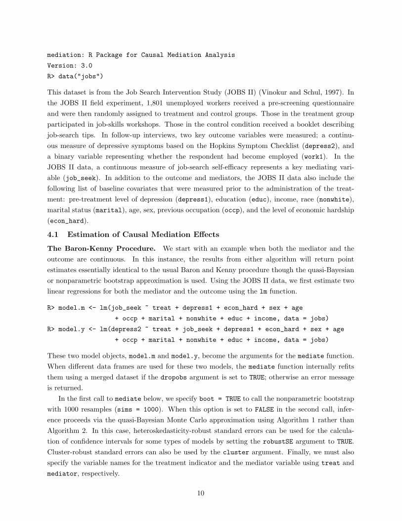
4.1 Estimation of Causal Mediation Effects
The Baron-Kenny Procedure. We start with an example when both the mediator and the
outcome are continuous. In this instance, the results from either algorithm will return point
estimates essentially identical to the usual Baron and Kenny procedure though the quasi-Bayesian
or nonparametric bootstrap approximation is used. Using the JOBS II data, we first estimate two
linear regressions for both the mediator and the outcome using the lm function.
R> model.m <- lm(job_seek ~ treat + depress1 + econ_hard + sex + age
+ occp + marital + nonwhite + educ + income, data = jobs)
R> model.y <- lm(depress2 ~ treat + job_seek + depress1 + econ_hard + sex + age
+ occp + marital + nonwhite + educ + income, data = jobs)
These two model objects, model.m and model.y, become the arguments for the mediate function.
When different data frames are used for these two models, the mediate function internally refits
them using a merged dataset if the dropobs argument is set to TRUE; otherwise an error message
is returned.
In the first call to mediate below, we specify boot = TRUE to call the nonparametric bootstrap
with 1000 resamples (sims = 1000). When this option is set to FALSE in the second call, infer-
ence proceeds via the quasi-Bayesian Monte Carlo approximation using Algorithm 1 rather than
Algorithm 2. In this case, heteroskedasticity-robust standard errors can be used for the calcula-
tion of confidence intervals for some types of models by setting the robustSE argument to TRUE.
Cluster-robust standard errors can also be used by the cluster argument. Finally, we must also
specify the variable names for the treatment indicator and the mediator variable using treat and
mediator, respectively.
10

R> out.1 <- mediate(model.m, model.y, sims = 1000, boot = TRUE, treat = "treat",
mediator = "job_seek")
R> out.2 <- mediate(model.m, model.y, sims = 1000, treat = "treat",
mediator = "job_seek")
The objects from a call to mediate, i.e., out.1 and out.2 above, are lists of class "mediate" which
contain several different quantities from the analysis. For example, out.1$d0 returns the point
estimate for the average causal mediation effect based on Algorithm 1. The help file contains a full
list of values that are contained in mediate objects.
The summary function prints out the results of the analysis in tabular form:
R> summary(out.2)
Causal Mediation Analysis
Quasi-Bayesian Confidence Intervals
Mediation Effect: -0.01375 95 % CI -0.031812 0.003299
Direct Effect: -0.03873 95 % CI -0.11938 0.04668
Total Effect: -0.05247 95 % CI -0.13431 0.03150
Proportion of Total Effect via Mediation: 0.2028 95 % CI -1.383 1.934
Sample Size Used: 899
The output from the summary function displays the estimates for the average causal mediation
effect, direct effect, total effect, and proportion of total effect mediated. The first column displays
the quantity of interest, the second column displays the point estimate, and the other columns
present the confidence intervals at the level specified by the conf.level argument which defaults
to 0.95. The number of observations used for the estimation is then displayed at the bottom. In
this case, we find that job search self-efficacy mediated the effect of the treatment on depression
in the negative direction. This effect, however, was small with a point estimate of −.014 and the
95% confidence interval (−.032,−.003) barely covers 0.
These results can be graphically presented by using the plot function:
R> plot(out.2)
The output is shown in Figure 2. The standard arguments for plot, such as titles (main, xlab,
etc.) and line widths (lwd), can be used and behave as expected.
The Baron-Kenny Procedure with the Interaction Term. Analysts can also allow the
causal mediation effect to vary with treatment status. Here, the model for the outcome must be
altered by including an interaction term between the treatment indicator, treat, and the mediator
variable, job_seek:
11
−0.15 −0.10 −0.05 0.00 0.05
●
●
●Total
Effect
DirectEffect
ACME
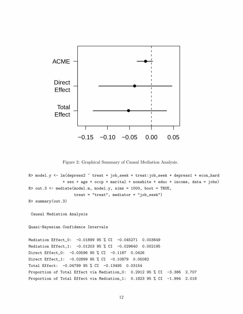
Figure 2: Graphical Summary of Causal Mediation Analysis.
R> model.y <- lm(depress2 ~ treat + job_seek + treat:job_seek + depress1 + econ_hard
+ sex + age + occp + marital + nonwhite + educ + income, data = jobs)
R> out.3 <- mediate(model.m, model.y, sims = 1000, boot = TRUE,
treat = "treat", mediator = "job_seek")
R> summary(out.3)
Causal Mediation Analysis
Quasi-Bayesian Confidence Intervals
Mediation Effect_0: -0.01899 95 % CI -0.045271 0.003649
Mediation Effect_1: -0.01203 95 % CI -0.029640 0.002195
Direct Effect_0: -0.03596 95 % CI -0.1187 0.0426
Direct Effect_1: -0.02899 95 % CI -0.10879 0.05082
Total Effect: -0.04799 95 % CI -0.13495 0.03154
Proportion of Total Effect via Mediation_0: 0.2912 95 % CI -3.386 2.707
Proportion of Total Effect via Mediation_1: 0.1823 95 % CI -1.994 2.018
12
Mediation Effect (Average): -0.01551 95 % CI -0.035757 0.003138
Direct Effect (Average): -0.03248 95 % CI -0.1129 0.0464
Proportion of Total Effect via Mediation (Average): 0.2381 95 % CI -2.867 2.443
Sample Size Used: 899
Again using the summary function provides a table of the results. Now estimates for the mediation
effects, direct effects and proportion of totel effect mediated correspond to the levels of the treatment
and are printed as such in the tabular summary. In this case, the mediation effect under the
treatment condition, listed as Mediation Effect_1 is estimated to be −.012 while the mediation
effect under the control condition, Mediation Effect_0, is −.019. The bottom of the table shows
the overall summary of these quantities averaged over the two treatment levels, as well as the
number of data points.
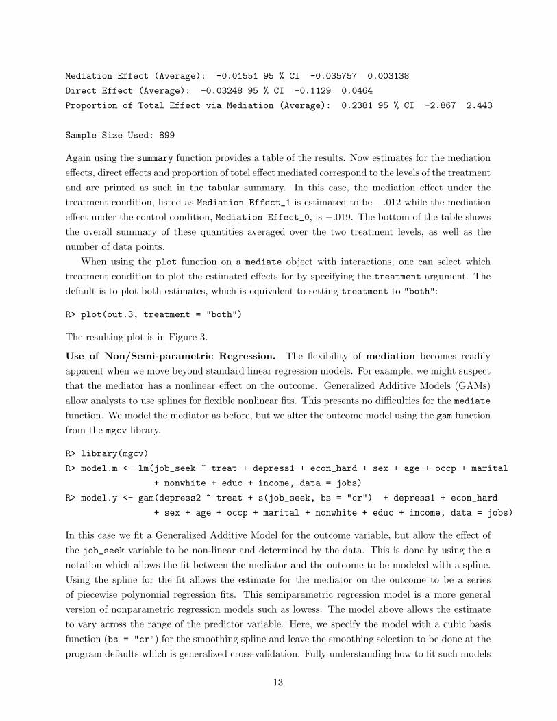
When using the plot function on a mediate object with interactions, one can select which
treatment condition to plot the estimated effects for by specifying the treatment argument. The
default is to plot both estimates, which is equivalent to setting treatment to "both":
R> plot(out.3, treatment = "both")
The resulting plot is in Figure 3.
Use of Non/Semi-parametric Regression. The flexibility of mediation becomes readily
apparent when we move beyond standard linear regression models. For example, we might suspect
that the mediator has a nonlinear effect on the outcome. Generalized Additive Models (GAMs)
allow analysts to use splines for flexible nonlinear fits. This presents no difficulties for the mediate
function. We model the mediator as before, but we alter the outcome model using the gam function
from the mgcv library.
R> library(mgcv)
R> model.m <- lm(job_seek ~ treat + depress1 + econ_hard + sex + age + occp + marital
+ nonwhite + educ + income, data = jobs)
R> model.y <- gam(depress2 ~ treat + s(job_seek, bs = "cr") + depress1 + econ_hard
+ sex + age + occp + marital + nonwhite + educ + income, data = jobs)
In this case we fit a Generalized Additive Model for the outcome variable, but allow the effect of
the job_seek variable to be non-linear and determined by the data. This is done by using the s
notation which allows the fit between the mediator and the outcome to be modeled with a spline.
Using the spline for the fit allows the estimate for the mediator on the outcome to be a series
of piecewise polynomial regression fits. This semiparametric regression model is a more general
version of nonparametric regression models such as lowess. The model above allows the estimate
to vary across the range of the predictor variable. Here, we specify the model with a cubic basis
function (bs = "cr") for the smoothing spline and leave the smoothing selection to be done at the
program defaults which is generalized cross-validation. Fully understanding how to fit such models
13

−0.15 −0.10 −0.05 0.00 0.05
●
●
●
●
●
TotalEffect
DirectEffect
ACME
Figure 3: Causal Mediation Analysis with Interaction between Treatment and Mediator.
is beyond the scope here. Interested readers should consult Wood (2006) for full technical details
and Keele (2008) provides coverage of these models from a social science perspective.
The call to mediate with a gam fit remains unchanged except that when the outcome model is
a semiparametric regression only the nonparametric bootstrap is valid for calculating uncertainty
estimates, i.e., boot = TRUE.
R> out.4 <- mediate(model.m, model.y, sims = 1000, boot = TRUE, treat = "treat",
mediator = "job_seek")
The model for the mediator can be modeled with the gam function as well. The gam function
also allows analysts to include interactions; thus analysts can still allow the mediation effects to
vary with treatment status. This simply requires altering the model specification by using the by
option in the gam function and using two separate indicator variables for treatment status. To fit
this model we need one variable that indicates whether the observation was in the treatment group
and a second variable that indicates whether the observation was in the control group. To allow
the mediation effect to vary with treatment status, the call to gam takes the following form:
R> model.y <- gam(depress2 ~ treat + s(job_seek, by = treat) + s(job_seek, by = control)
+ depress1 + econ_hard + sex + age + occp + marital + nonwhite + educ + income,
data = jobs)
14

In this case, we must also alter the options in the mediate function by providing the variable name
for the control group indicator using the control option.
R> out.5 <- mediate(model.m, model.y, sims = 1000, boot = TRUE,
treat = "treat", mediator = "job_seek", control = "control")
R> summary(out.5)
Causal Mediation Analysis
Confidence Intervals Based on Nonparametric Bootstrap
Mediation Effect_0: -0.02254 95 % CI -0.051956 0.004447
Mediation Effect_1: -0.0171 95 % CI -0.038895 0.002281
Direct Effect_0: -0.009742 95 % CI -0.09718 0.07924
Direct Effect_1: -0.004302 95 % CI -0.08926 0.08285
Total Effect: -0.02684 95 % CI -0.11932 0.06449
Proportion of Total Effect via Mediation_0: 0.3892 95 % CI -4.411 9.161
Proportion of Total Effect via Mediation_1: 0.2768 95 % CI -3.614 6.960
Mediation Effect (Average): -0.01982 95 % CI -0.045831 0.003105
Direct Effect (Average): -0.007022 95 % CI -0.09207 0.08178
Proportion of Total Effect via Mediation (Average): 0.3398 95 % CI -3.870 8.105
Sample Size Used: 899
Quantile Causal Mediation Effects. Researchers might also be interested in modeling media-
tion effects for quantiles of the outcome. Quantile regression allows for a convenient way to model
the quantiles of the outcome distribution while adjusting for a variety of covariates (Koenker, 2008).
For example, a researcher might be interested in the 0.5 quantile (i.e., median) of the distribution.
This also presents no difficulties for the mediate function. Again for these models, uncertainty
estimates are calculated using the nonparametric bootstrap. To use quantile regression, we use the
rq function in package quantreg and model the median of the outcome, though other quantiles are
also permissible. Analysts can also relax the no-interaction assumption for the quantile regression
models as well. Below we estimate the mediator with a standard linear regression, while for the
outcome we use rq to model the median.
R> library(quantreg)
R> model.m <- lm(job_seek ~ treat + depress1 + econ_hard + sex + age + occp + marital
+ nonwhite + educ + income, data = jobs)
R> model.y <- rq(depress2 ~ treat + job_seek + depress1 + econ_hard + sex
+ age + occp + marital + nonwhite + educ + income,
tau = 0.5, data = jobs)
15
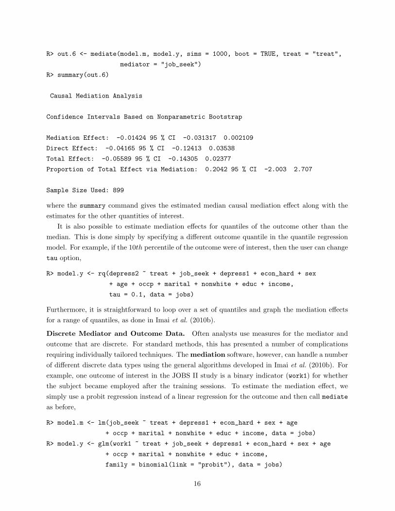
R> out.6 <- mediate(model.m, model.y, sims = 1000, boot = TRUE, treat = "treat",
mediator = "job_seek")
R> summary(out.6)
Causal Mediation Analysis
Confidence Intervals Based on Nonparametric Bootstrap
Mediation Effect: -0.01424 95 % CI -0.031317 0.002109
Direct Effect: -0.04165 95 % CI -0.12413 0.03538
Total Effect: -0.05589 95 % CI -0.14305 0.02377
Proportion of Total Effect via Mediation: 0.2042 95 % CI -2.003 2.707
Sample Size Used: 899
where the summary command gives the estimated median causal mediation effect along with the
estimates for the other quantities of interest.
It is also possible to estimate mediation effects for quantiles of the outcome other than the
median. This is done simply by specifying a different outcome quantile in the quantile regression
model. For example, if the 10th percentile of the outcome were of interest, then the user can change
tau option,
R> model.y <- rq(depress2 ~ treat + job_seek + depress1 + econ_hard + sex
+ age + occp + marital + nonwhite + educ + income,
tau = 0.1, data = jobs)
Furthermore, it is straightforward to loop over a set of quantiles and graph the mediation effects
for a range of quantiles, as done in Imai et al. (2010b).
Discrete Mediator and Outcome Data. Often analysts use measures for the mediator and
outcome that are discrete. For standard methods, this has presented a number of complications
requiring individually tailored techniques. The mediation software, however, can handle a number
of different discrete data types using the general algorithms developed in Imai et al. (2010b). For
example, one outcome of interest in the JOBS II study is a binary indicator (work1) for whether
the subject became employed after the training sessions. To estimate the mediation effect, we
simply use a probit regression instead of a linear regression for the outcome and then call mediate
as before,
R> model.m <- lm(job_seek ~ treat + depress1 + econ_hard + sex + age
+ occp + marital + nonwhite + educ + income, data = jobs)
R> model.y <- glm(work1 ~ treat + job_seek + depress1 + econ_hard + sex + age
+ occp + marital + nonwhite + educ + income,
family = binomial(link = "probit"), data = jobs)
16

R> out.7 <- mediate(model.m, model.y, sims = 1000, treat = "treat",
mediator = "job_seek")
R> summary(out.7)
Causal Mediation Analysis
Quasi-Bayesian Confidence Intervals
Mediation Effect_0: 0.003290 95 % CI -0.0009537 0.0098747
Mediation Effect_1: 0.003538 95 % CI -0.001052 0.010728
Direct Effect_0: 0.05514 95 % CI -0.006427 0.113568
Direct Effect_1: 0.05538 95 % CI -0.006487 0.114191
Total Effect: 0.05867 95 % CI -0.003816 0.117091
Proportion of Total Effect via Mediation_0: 0.0455 95 % CI -0.0768 0.4070
Proportion of Total Effect via Mediation_1: 0.05042 95 % CI -0.0777 0.4110
Mediation Effect (Average): 0.003414 95 % CI -0.001003 0.010269
Direct Effect (Average): 0.05526 95 % CI -0.006457 0.113879
Proportion of Total Effect via Mediation (Average): 0.04802 95 % CI -0.07725 0.41005
Sample Size Used: 899
In the table printed by the summary function, the estimated average causal mediation effect
along with the quasi-Bayesian confidence interval are printed on the first line followed by the direct
and total effects, and the proportion of the total effect due to mediation. Even though the outcome
model does not include an interaction term between the treatment and mediator, the estimated
effects slightly differ between the treatment and control conditions. This difference, however, is
solely due to the nonlinearity in the outcome model and should be extremely small. It is also
possible to use a logit model for the outcome instead of a probit model. However, we recommend
the use of a probit model because our implementation of the sensitivity analysis below requires a
probit model for analytical tractability.
The mediator can also be binary or ordered measures as well. This simply requires modeling
the mediator with either a probit or ordered probit model. For demonstration purposes, the jobs
data contains two variables, job_dich and job_disc, which are recoded versions of job_seek.
The first measure is simply the continuous scale divided at the median into a binary variable.
The second measure, job_disc, recodes the continuous scale into a discrete four point scale. We
emphasize that this is for demonstration purposes only, and analysts in general should not recode
continuous measures into discrete measures. Estimating mediation effects with a binary mediator
is quite similar to the case above with a binary outcome. We simply now use a probit model for
the mediator and a linear regression for the outcome,
17

R> model.m <- glm(job_dich ~ treat + depress1 + econ_hard + sex + age
+ occp + marital + nonwhite + educ + income, data = job,
family = binomial(link = "probit"))
R> model.y <- lm(depress2 ~ treat + job_dich + treat:job_dich + depress1
+ econ_hard + sex + age + occp + marital + nonwhite
+ educ + income, data = jobs)
In this example we include the interaction term between the treatment and mediator to allow
the effect of the mediator to vary with treatment status. The user now calls mediate and can use
either the quasi-Bayesian approximation or nonparametric bootstrap.
R> out.8 <- mediate(model.m, model.y, sims = 1000, treat = "treat",
mediator = "job_dich")
R> summary(out.8)
Causal Mediation Analysis
Quasi-Bayesian Confidence Intervals
Mediation Effect_0: -0.01823 95 % CI -0.038944 -0.002616
Mediation Effect_1: -0.02040 95 % CI -0.038965 -0.003155
Direct Effect_0: -0.02823 95 % CI -0.10786 0.05154
Direct Effect_1: -0.03039 95 % CI -0.11164 0.04764
Total Effect: -0.04863 95 % CI -0.13146 0.02839
Proportion of Total Effect via Mediation_0: 0.2782 95 % CI -3.055 3.325
Proportion of Total Effect via Mediation_1: 0.3162 95 % CI -3.443 3.628
Mediation Effect (Average): -0.01932 95 % CI -0.037878 -0.003201
Direct Effect (Average): -0.02931 95 % CI -0.11052 0.04807
Proportion of Total Effect via Mediation (Average): 0.301 95 % CI -3.016 3.477
Sample Size Used: 899
In the table, we see that Mediation Effect_0 is the mediation effect under the control condition,
while Mediation Effect_1 is the mediation effect under the treatment condition. The same nota-
tion applies to the direct effects. As the reader can see, the output also indicates which algorithm
is used for the 95% confidence intervals.
When the mediator is an ordered variable, we switch to an ordered probit model for the medi-
ator. In R, the polr function in the MASS library provides this functionality. (Alternatively, the
bayespolr function in the arm library can also be used.) Thus, we fit the outcome and mediator
models below,
R> model.m <- polr(job_disc ~ treat + depress1 + econ_hard + sex + age
18

+ occp + marital + nonwhite + educ + income,
data = jobs, method = "probit", Hess = TRUE)
R> model.y <- lm(depress2 ~ treat + job_disc + depress1 + econ_hard + sex + age
+ occp + marital + nonwhite + educ + income, data = jobs)
The reader should note that in the call to polr the Hess = TRUE should be specified to compute the
asymptotic variance covariance matrix for the estimated model coefficients in the quasi-Bayesian
approximation. Otherwise, the Hessian of the log-likelihood will be recalculated within the mediate
call.
Once we have estimated these two models, analysis proceeds as before,
R> out.9 <- mediate(model.m, model.y, sims = 1000, treat = "treat",
mediator = "job_disc")
R> summary(out.9)
Causal Mediation Analysis
Quasi-Bayesian Confidence Intervals
Mediation Effect: -0.01048 95 % CI -0.03188 0.01008
Direct Effect: -0.03311 95 % CI -0.10759 0.04848
Total Effect: -0.04360 95 % CI -0.12376 0.03895
Proportion of Total Effect via Mediation: 0.1726 95 % CI -2.752 2.077
Sample Size Used: 899
Again, for any of these data types, analysts can relax the no-interaction assumption as before by
including the interaction between treatment and the mediator variable in the outcome model.
4.2 Sensitivity Analysis
Once analysts have estimated mediation effects, they should explore how robust their finding is to
the ignorability assumption, whenever possible. The medsens function allows analysts to conduct
sensitivity analyses for mediation effects as well as direct effects. In this section we provide a
demonstration of these functionalities. Currently, mediation can conduct sensitivity analyses
when both mediator and outcome are continuous and modelled with the lm function, as well as
when either mediator or outcome (but not both) is binary and modelled using a binary probit
regression via glm.
The Baron-Kenny Procedure. As before, one must first fit models for the mediator and
outcome and then pass these model objects through the mediate function:
R> model.m <- lm(job_seek ~ treat + depress1 + econ_hard + sex + age + occp
+ marital + nonwhite + educ + income, data = jobs)
19

R> model.y <- lm(depress2 ~ treat + job_seek + depress1 + econ_hard + sex + age + occp
+ marital + nonwhite + educ + income, data = jobs)
R> med.cont <- mediate(model.m, model.y, sims=1000, treat = "treat",
mediator = "job_seek")
Once the analyst estimates the mediation effects, the output from the mediate function becomes
the argument for medsens, which is the workhorse function. The medsens function recognizes main
arguments specified in the mediate function and thus there is no need to specify options such as
treat or mediator.
R> sens.cont <- medsens(med.cont, rho.by = 0.05)
The rho.by option specifies how finely incremented the parameter ρ is for the sensitivity analysis.
When ρ is on a coarser grid, this speeds up estimation considerably but comes at the cost of
estimating the robustness of the original conclusion only imprecisely.
After running the sensitivity analysis via medsens, the summary function can be used to produce
a table with the values of ρ for which the confidence interval contains zero. This allows the analyst
to immediately see the approximate range of ρ where the sign of the causal mediation effect is
indeterminate. The second section of the table contains the value of ρ for which the mediation
effect is exactly zero, which in this application is −0.19. The table also presents coefficients of
determination that correspond to the critical value of ρ where the mediation effect is zero. First,
R∗2MR∗2
Y is the product of coefficients of determination which represents the proportion of the
previously unexplained variance in the mediator and outcome variables that is explained by an
unobservable pretreatment unconfounder. An alternative formulation is in terms of the proportion
of the original variance explained by an unobserved confounder, which we denote as R̃2M R̃2
Y .
R> summary(sens.cont)
Mediation Sensitivity Analysis for Average Causal Mediation Effect
Sensitivity Region
Rho Med. Eff. 95% CI Lower 95% CI Upper R^2_M*R^2_Y* R^2_M~R^2_Y~
[14,] -0.30 0.0064 -0.0025 0.0153 0.0900 0.0588
[15,] -0.25 0.0028 -0.0026 0.0082 0.0625 0.0408
[16,] -0.20 -0.0007 -0.0049 0.0036 0.0400 0.0261
[17,] -0.15 -0.0040 -0.0105 0.0025 0.0225 0.0147
Rho at which ACME = 0: -0.2
20

R^2_M*R^2_Y* at which ACME = 0: 0.04
R^2_M~R^2_Y~ at which ACME = 0: 0.0261
The table above presents the estimated mediation effect along with its confidence interval for each
value of ρ. The reader can verify that when ρ is equal to zero, the reported mediation effect
matches the estimate produced by the mediate function. For other values of ρ, the mediation
effect is calculated under different levels of unobserved confounding.
The information from the sensitivity analysis can also be summarized graphically using the
plot function. First, passing the medsens object to plot and specifying the sens.par option to
"rho", i.e.,
R> plot(sens.cont, sens.par = "rho")
produces the left hand side of Figure 4. In the plot, the dashed horizontal line represents the esti-
mated mediation effect under the sequential ignorability assumption, and the solid line represents
the mediation effect under various values of ρ. The grey region represents the 95% confidence
bands.
Similarly, we can also plot the sensitivity analysis in terms of the coefficients of determination as
discussed above. Here we specify sens.par option to "R2". We also need to specify two additional
pieces of information. First, r.type option tells the plot function whether to plot R∗2MR∗2
Y or
R̃2M R̃2
Y . To plot the former r.type is set to "residual" and to plot the latter r.type is set to
"total". Finally, the sign.prod option specifies the sign of the product of the coefficients of
the unobserved confounder in the mediator and outcome models. This product indicates whether
the unobserved confounder affects both mediator and outcome variables in the same direction
("positive") or different directions ("negative"), thereby reflecting the analyst’s expectation
about the nature of confounding.
For example, the following command produces the plot representing the sensitivity of estimates
with respect to the proportion of the original variances explained by the unobserved confounder
when the confounder is hypothesized to affect the mediator and outcome variables in opposite
directions.
R> plot(sens.cont, sens.par = "R2", r.type = "total", sign.prod = "negative")
The resulting plot is shown on the right hand side of Figure 4. Each contour line represents
the mediation effect for the corresponding values of R̃2M and R̃2
Y . For example, the 0 contour
line corresponds to values of the product R̃2M R̃2
Y such that the ACME is 0. As reported in the
table, even a small proportion of original variance unexplained by the confounder, .02%, produces
mediation effects of 0. Accordingly, the right hand side of Figure 4 shows how increases in R̃2M R̃2
Y
(moving from the lower left to upper right) produce positive mediation effects.
21

−1.0 −0.5 0.0 0.5 1.0
−0.
2−
0.1
0.0
0.1
ACME(ρ)
Sensitivity Parameter: ρ
Ave
rage
Med
iatio
n E
ffect
: δ(t)
ACME(R~
M2
,R~
Y2), sgn(λ2λ3) = −1
0
0.02
0.04
0.06
0.08
0.0 0.2 0.4 0.6 0.8 1.0
0.0
0.2
0.4
0.6
0.8
1.0
R~
M2
R~Y2
0.0
0.1
0.2
0.3
0.4
0.5
0.6
0.7
0.8
0.9
1.0
0.0 0.2 0.4 0.6 0.8 1.0
Figure 4: Sensitivity Analysis with Continuous Outcome and Mediator.
For both types of sensitivity plots, the user can specify additional options available in the
plot function such as alternative title (main) and axis labels (xlab, ylab) or manipulate common
graphical options (e.g., xlim).
Binary Outcome. The medsens function also extends to analyses where the mediator is binary
and the outcome is continuous, as well as when the mediator is continuous and the outcome is
binary. If either variable is binary, medsens takes an additional argument. For example, recall the
binary outcome model estimated earlier:
R> model.y <- glm(work1 ~ treat + job_seek + depress1 + econ_hard + sex + age
+ occp + marital + nonwhite + educ + income,
family = binomial(link = "probit"), data = jobs)
R> med.bout <- mediate(model.m, model.y, sims = 1000, treat = "treat",
mediator = "job_seek")
The call to medsens works as before, with the output from the mediate function passed through
medsens.
R> sens.bout <- medsens(med.bout, rho.by = 0.05, sims = 1000)
The sims option provides control over the number of Monte Carlo draws used to compute con-
fidence bands. When either the mediator or outcome is binary, the exact values of sensitivity
parameters where the mediation effects are zero cannot be analytically obtained as in the fully
continuous case (see Imai et al., 2010c, Section 4). Thus, this information is reported based on the
signs of the estimated mediation effects under various values of ρ and corresponding coefficients of
determination. The usage of the summary function, however, remains identical to the fully contin-
uous case in that the output table contains the estimated mediation effects and the corresponding
values of ρ for which the confidence region contains zero.
As in the case with continuous mediator and outcome variables, we can plot the results of the
sensitivity analysis. The following code produces Figure 5.
22

−1.0 −0.5 0.0 0.5 1.0
−0.
050.
000.
050.
10
ACME0(ρ)
Sensitivity Parameter: ρ
Ave
rage
Med
iatio
n E
ffect
: δ(0
)
−1.0 −0.5 0.0 0.5 1.0
−0.
050.
000.
050.
10
ACME1(ρ)
Sensitivity Parameter: ρ
Ave
rage
Med
iatio
n E
ffect
: δ(1
)
ACME0(R~
M
2,R~
Y
2), sgn(λ2λ3) = 1
−0.04 −0.03
−0.02
−0.01
0
0.0 0.2 0.4 0.6 0.8 1.0
0.0
0.2
0.4
0.6
0.8
1.0
R~
M
2
R~Y2
0.0
0.2
0.4
0.6
0.8
1.0
0.0 0.2 0.4 0.6 0.8 1.0
ACME1(R~
M
2,R~
Y
2), sgn(λ2λ3) = 1
−0.05 −0.04
−0.03
−0.02
−0.01
0
0.0 0.2 0.4 0.6 0.8 1.0
0.0
0.2
0.4
0.6
0.8
1.0
R~
M
2
R~Y2
0.0
0.2
0.4
0.6
0.8
1.0
0.0 0.2 0.4 0.6 0.8 1.0
Figure 5: Sensitivity Analysis with Continuous Outcome and Binary Mediator.
R> plot(sens.bout, sens.par = "rho")
R> plot(sens.bout, sens.par = "R2", r.type = "total", sign.prod = "positive")
On the left hand side we plot the ACME in terms of ρ, while we plot the ACME in terms of R̃2M
and R̃2Y on the right hand side. In the ρ plot, the dashed line represents the estimated mediation
effect under sequential ignorability, and the solid line represents the mediation effect under various
values of ρ. The grey region represents the 95% confidence bands. In the R̃2 plot the ACME is
plotted against various values of R̃2M and R̃2
Y and is interpreted in the same way as above.
When the outcome is binary, the proportion of the the total effect due to mediation can also be
calculated as function of the sensitivity parameter ρ. The pr.plot option in the plot command (in
conjunction with the sens.par = "rho" option) allows users to plot a summary of the sensitivity
analysis for the proportion mediated. For example, the following call would provide a plot of this
quantity:
R> plot(sens.bout, sens.par = "rho", pr.plot = TRUE)
Binary Mediator. The final form of sensitivity analysis deals with the case where the outcome
variable is continuous but the mediator is binary. For the purpose of illustration, we simply
dichotomize the job_seek variable to produce a binary measure job_dich. We fit a probit model
for the mediator and linear regression for the outcome variable.
23

−1.0 −0.5 0.0 0.5 1.0
−0.
06−
0.04
−0.
020.
000.
02
ACME(ρ)
Sensitivity Parameter: ρ
Ave
rage
Med
iatio
n E
ffect
: δ(t)
Figure 6: Sensitivity Analysis with Continuous Outcome and Binary Mediator.
R> model.m <- glm(job_dich ~ treat + depress1 + econ_hard + sex + age
+ occp + marital + nonwhite + educ + income,
data = jobs, family = binomial(link = "probit"))
R> model.y <- lm(depress2 ~ treat + job_dich+ depress1 + econ_hard + sex + age
+ occp + marital + nonwhite + educ + income, data = jobs)
R> med.bmed <- mediate(model.m, model.y, sims = 1000, treat = "treat",
mediator = "job_dich")
R> sens.bmed <- medsens(med.bmed, rho.by = 0.05, sims = 1000)
Again we can pass the output of the medsens function through the plot function,
R> plot(sens.bmed, sens.par = "rho")
producing Figure 6. The plot is interpreted in the same way as the above cases. The user also has
the option to plot sensitivity results in terms of the coefficients of determination just as in the case
with continuous outcome and mediator variables.
When the mediator variable is binary, the plotted values of the mediation effect and their
confidence bands may not be perfectly smooth curves due to simulation errors. This is especially
likely when the number of simulations (sims) is set to a small value. In such situations, the user
24

can choose to set the smooth.effect and smooth.ci options to TRUE in the plot function so
that the corresponding values become smoothed out via a lowess smoother before being plotted.
Although this option often makes the produced graph look nicer, the user should be cautious as
the adjustment could affect one’s substantive conclusions in a significant way. A recommended
alternative is to increase the number of simulations.
5 Multiple Causal Mediation Analyses via mediations
Researchers may face a situation where they want to conduct multiple causal mediation analyses.
For example, the researcher may have run several different experiments that had different treatment
conditions but had the same mediator and outcome variables. Or, a researcher may measure several
different mediating variables in their experiment and wish to estimate causal mediation effects for
each of these cases. In these situations the researcher would need to write separate lines of code
for the different models. A more efficient way is to loop over the different combinations of interest.
The mediations function facilitates this process.
The mediations function can be used to conduct causal mediation analyses over the range of
treatment, mediator, and outcome combinations that could be present within a study. For example,
if there were two treatment conditions, two measured mediators, and two outcomes, mediations
would run eight causal mediation analyses. The results can then be analyzed with the summary and
plot functions. If there is only one treatment variable, the user needs only a single data set that
contains all mediators and outcomes of interest. If there are multiple treatment variables, then the
researcher must first create separate data frames, each with all mediator/outcome variables to be
considered, and named using a convention where the name of the data frame object begins with
the name of the treatment variable contained within it.
Use of the mediations function is straightforward. First, the user creates vectors of the treat-
ment, mediator, outcome, and covariates names that are to be used. The treatment, mediator, and
outcome variables are looped over to produce all possible combinations of mediator and outcome
models. The set of covariates is held constant across the models. The different model combinations
are then entered into the mediate function.
The user can specify several different options for mediations. First, the type of model to be
used for the mediator and outcome equations must be specified. Currently, mediations can handle
a variety of different model combinations. Either the mediator or outcome equation can be modeled
with linear regression, probit, ordered probit, and quantile regression. The mediations function
also handles the case where tobit is used for the outcome. Next, the user must also specify the
standard features that are necessary for the mediate function, such as the number of simulations
(sims). In addition, if quantile regression or tobit regression is used, the user needs to specify
the appropriate parameters, such as the quantiles to be estimated (tau.m, tau.y) and cutpoints
(LowerY, UpperY). If the user wishes for estimates to include weights (e.g., survey weights) then
the name of the weight variable needs to be passed via the weights argument.
The output of mediations contains a collection of mediate objects. The naming system uses
the name of the particular outcome variable, mediator, and treatment, each separated by a dot.
25
For example, if the output of mediations is output and the outcome, mediator and treatment
variable names O, M1 or M2, and T, respectively, then output$O.M2.T would be the mediate object
from using mediator M2.
There are several limitations to the code. First, it works only with a subset of the model types
that will be accommodated if mediate is used individually. Second, one cannot specify separate sets
of covariates for different treatment/mediator/outcome combinations. Users should use mediate
separately for individual models if more flexibility is required in their specific applications.
While mediations is a helpful function, it is also easy to abuse. First, researchers must be aware
of the assumptions being made at every step of causal mediation analysis. For example, if there are
multiple mediators, a strong assumption must be made for the estimates to be interpreted as causal
quantities. One such assumption is that the mediators are not causally related. Second, care must
be taken against the risks of multiple testing when a large number of treatment/mediator/outcome
combinations are involved. The mediations function simply runs independent mediate processes
and does not use any correction procedures for multiple testing, so the confidence intervals may be
too narrow. We recommend that the use of this function be limited for exploratory analyses.
An illustration of the mediations function can be found in the Examples section of its help
document; see ?mediations or example(mediations).
6 Concluding Remarks
Causal mediation analysis is a key tool for social scientific research. In this paper, we describe our
easy-to-use software for causal mediation analysis, mediation, that implements the new methods
and algorithms introduced by Imai, Keele, and Yamamoto (2010c) and Imai, Keele, and Tingley
(2010b). The software provides a flexible, unified approach to causal mediation analysis in various
situations encountered by applied researchers. The object-oriented nature of the R programming
made it possible for us to implement these algorithms in a fairly general way. In addition to
the estimation of causal mediation effects, mediation implements formal sensitivity analyses so
that researchers can assess the robustness of their findings to the potential violations of the key
identifying assumption. This is an important contribution for at least two reasons. First, even
in randomized experiments, causal mediation analysis requires an additional assumption that is
not directly testable from the observed data. Thus, researchers must evaluate the consequences of
potential violations of the assumption via sensitivity analysis. Second, the accumulation of such
sensitivity analyses is essential for interpreting the relative degree of robustness across different
studies. Thus, the development of easy-to-use software, such as mediation, facilitates causal
mediation analysis in applied social science research in several critical directions.
26

References
Imai, K., Keele, L., Tingley, D., and Yamamoto, T. (2010a). Advances in Social Science Research
Using R (ed. H. D. Vinod), chapter Causal Mediation Analysis Using R, pages 129–154. Lecture
Notes in Statistics. Springer, New York.
Imai, K., Keele, L., and Tingley, D. (2010b). A general approach to causal mediation analysis.
Psychological Methods, 15(4), 309–334.
Imai, K., Keele, L., and Yamamoto, T. (2010c). Identification, inference, and sensitivity analysis
for causal mediation effects. Statistical Science, 25(1), 51–71.
Keele, L. (2008). Semiparametric Regression for the Social Sciences. Wiley and Sons, Chichester,
UK.
King, G., Tomz, M., and Wittenberg, J. (2000). Making the most of statistical analyses: Improving
interpretation and presentation. American Journal of Political Science, 44(2), 341–355.
Koenker, R. (2008). Quantile Regression. Cambridge University Press, Cambridge.
Mackinnon, D., Lockwood, C., and Williams, J. (2004). Confidence limits for the indirect effect:
Distribution of the product and resampling methods. Multivariate Behavioral Research, 39(1),
99–129.
Preacher, K. and Hayes, A. (2008). Asymptotic and resampling strategies for assessing and com-
paring indirect effects in multiple mediator models. Behavioral Research Methods, 40, 879–891.
R Development Core Team (2009). R: A Language and Environment for Statistical Computing . R
Foundation for Statistical Computing, Vienna, Austria. ISBN 3-900051-07-0.
Rosenbaum, P. R. (2002). Observational Studies. Springer-Verlag, New York, 2nd edition.
Vinokur, A. and Schul, Y. (1997). Mastery and inoculation against setbacks as active ingredients in
the jobs intervention for the unemployed. Journal of Consulting and Clinical Psychology , 65(5),
867–877.
Wood, S. (2006). Generalized Additive Models: An Introduction With R. Chapman & Hall/CRC,
Boca Raton.
Zellner, A. (1962). An efficient method of estimating seemingly unrelated regressions and tests for
aggregation bias. Journal of the American Statistical Association, 57, 348–368.
27