causes and consequences of the late 1960s great salinity ... · causes and consequences of the late...

10

Causes and Consequences of the Late 1960s Great Salinity Anomaly

Mihai Dima1 and Gerrit Lohmann2

1University of Bucharest, Faculty of Physics 2Alfred Wegener Institute for Polar and Marine Research

1Romania 2Germany

1. Introduction

The second half of the 20th century showed a series of decadal-scale anomalies of salinity, temperature and sea ice cover in the northern North Atlantic. One pronounced event, the 'great salinity anomaly' (GSA) is observed in the late 1060s and the early 1970s (Dickson et al., 1988). This anomaly can be linked to the sea ice volume out of the Arctic through Fram Strait, which represents a major source of freshwater (Aagaard & Carmack, 1989; Schmith & Hansen, 2003). Increased sea ice export from the Arctic Ocean stabilizes the upper water column in the North Atlantic, diminishes the production of intermediate and deep water masses through ocean convection and can influence the large-scale ocean circulation (Häkkinen, 1999). An important part of sea ice export from the Arctic is forced by specific atmospheric structures (Hilmer et al., 1998; Häkkinen and Geiger, 2000; Cavalieri 2002). These can be parts of coupled ocean-atmosphere modes of climate variability with large-scale projections. The large-scale Atlantic meridional overturning circulation (AMOC) is a key component of the climate system. It can be defined as the part of the global ocean circulation, which is driven by density differences. The relatively dense surface waters in the North Atlantic generate downward mixing and southward movement of deep-water masses. This is partially balanced by a transport of saline waters by surface ocean currents from the tropics to midlatitudes. Changes in the AMOC can be very abrupt and have a worldwide climatic impact as demonstrated in theoretical and numerical studies (Stommel, 1961; Rahmstorf, 1994). There is significant evidence that the past abrupt climate changes (Dansgaard et al., 1993; Heinrich, 1988) were linked to AMOC variations (EPICA, 2006). One of the largest climate changes during the last 10.000 years occurred about 8.200 years ago (Alley, 2001) and it had a large impact over the Northern Hemisphere. It was proposed that this event included a freshwater pulse entering the North Atlantic (Barber et al., 1999) and modeling simulations suggest that it was associated with AMOC reduction (Renssen et al., 2002). Given the prominence of the GSA and its potential worldwide impact through the AMOC, it is of significant importance to understand the physical mechanisms associated to this outstanding climatic anomaly. Therefore, the goal of this study is to investigate the causes and the consequences of the GSA. The "climate mode" represents an useful concept to reduce the complexity of climate variations and can be defined as a set of physical processes with coherent spatial variability and quasi-periodic variations in time. Based on North Atlantic sea ice and sea level pressure

www.intechopen.com

Planet Earth 2011 – Global Warming Challenges and Opportunities for Policy and Practice

214

(SLP) data for the 1903-1994 period, it was noted that the constructive inference between four interannual-to-interdecadal modes may be responsible for the GSA (Venegas & Mysak, 2000). This observation is further investigated here based on a reconstruction of the sea ice export through Fram Strait (Fram Strait Sea Ice Export - FSSIE), which extends back in time to 1820. Further more, a possible impact of the GSA on the AMOC is also presented. The identification of the quasi-periodic components in the FSSIE time series is presented in sections 2 and 3, and their physical relevance is addressed in section 4. The possible GSA impact on AMOC is presented in section 5. The 6th part of this study contains a summary and the conclusions.

2. Possible causes of the GSA

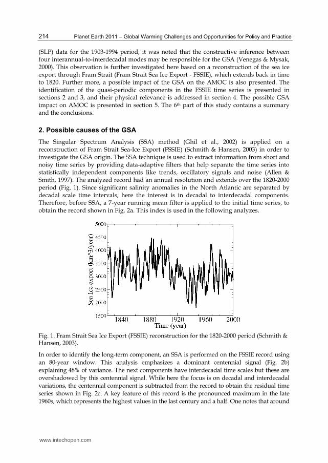
The Singular Spectrum Analysis (SSA) method (Ghil et al., 2002) is applied on a reconstruction of Fram Strait Sea-Ice Export (FSSIE) (Schmith & Hansen, 2003) in order to investigate the GSA origin. The SSA technique is used to extract information from short and noisy time series by providing data-adaptive filters that help separate the time series into statistically independent components like trends, oscillatory signals and noise (Allen & Smith, 1997). The analyzed record had an annual resolution and extends over the 1820-2000 period (Fig. 1). Since significant salinity anomalies in the North Atlantic are separated by decadal scale time intervals, here the interest is in decadal to interdecadal components. Therefore, before SSA, a 7-year running mean filter is applied to the initial time series, to obtain the record shown in Fig. 2a. This index is used in the following analyzes.

Fig. 1. Fram Strait Sea Ice Export (FSSIE) reconstruction for the 1820-2000 period (Schmith & Hansen, 2003).

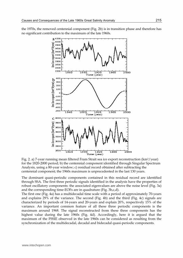
In order to identify the long-term component, an SSA is performed on the FSSIE record using

an 80-year window. This analysis emphasizes a dominant centennial signal (Fig. 2b)

explaining 48% of variance. The next components have interdecadal time scales but these are

overshadowed by this centennial signal. While here the focus is on decadal and interdecadal

variations, the centennial component is subtracted from the record to obtain the residual time

series shown in Fig. 2c. A key feature of this record is the pronounced maximum in the late

1960s, which represents the highest values in the last century and a half. One notes that around

www.intechopen.com


215

the 1970s, the removed centennial component (Fig. 2b) is in transition phase and therefore has

no significant contribution to the maximum of the late 1960s.

Fig. 2. a) 7-year running mean filtered Fram Strait sea ice export reconstruction (km3/year) for the 1820-2000 period; b) the centennial component identified through Singular Spectrum Analysis, using a 80-year window; c) residual record obtained after subtracting the centennial component; the 1960s maximum is unprecedented in the last 130 years.

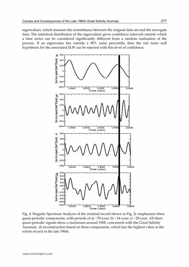
The dominant quasi-periodic components contained in this residual record are identified through SSA. The first three periodic signals identified in the analysis have the properties of robust oscillatory components: the associated eigenvalues are above the noise level (Fig. 3a) and the corresponding time-EOFs are in quadrature (Fig. 3b,c,d). The first one (Fig. 4a) has a multidecadal time scale with a period of approximately 70-years and explains 29% of the variance. The second (Fig. 4b) and the third (Fig. 4c) signals are characterized by periods of 14-years and 20-years and explain 20%, respectively 15% of the variance. An important common feature of all these three periodic components is the maximum around 1968. The signal reconstructed from these three components has the highest value during the late 1960s (Fig. 4d). Accordingly, here it is argued that the maximum of the FSSIE observed in the late 1960s can be considered as resulting from the synchronization of the multidecadal, decadal and bidecadal quasi-periodic components.

www.intechopen.com


216

Fig. 3. Singular Spectrum Analysis of the residual record shown in Fig. 2c, using a 80-year window. a) the eigenvalues spectrum; b) the time-EOFs 1 and 2; c) the time-EOFs 3 and 4 d) the time-EOFs 5 and 6. The robustness of the first three quasi-periodic components is supported by their distinction from the noise level in the eigenvalues spectrum and by the constant phase-lag of their associated time-EOFs.

3. Robustness of the quasi-periodic components

The significance of these components is further investigated through Monte Carlo simulations (Allen & Smith, 1997; Ghil et al., 2002). An ensemble of surrogate data is generated and a covariance matrix is computed for each realization. These matrices are projected onto the eigenvector basis of the original data to derive the corresponding

www.intechopen.com


217

eigenvalues, which measure the resemblance between the original data set and the surrogate data. The statistical distribution of the eigenvalues gives confidence intervals outside which a time series can be considered significantly different from a random realization of the process. If an eigenvalue lies outside a 90% noise percentile, then the red noise null hypothesis for the associated EOF can be rejected with this level of confidence.

Fig. 4. Singular Spectrum Analysis of the residual record shown in Fig. 2c emphasizes three quasi-periodic components, with periods of a) ~70-year; b) ~14-year; c) ~20-year. All three quasi-periodic signals show a maximum around 1968, concurrent with the Great Salinity Anomaly. d) reconstruction based on these components, which has the highest value in the whole record in the late 1960s.

www.intechopen.com


218

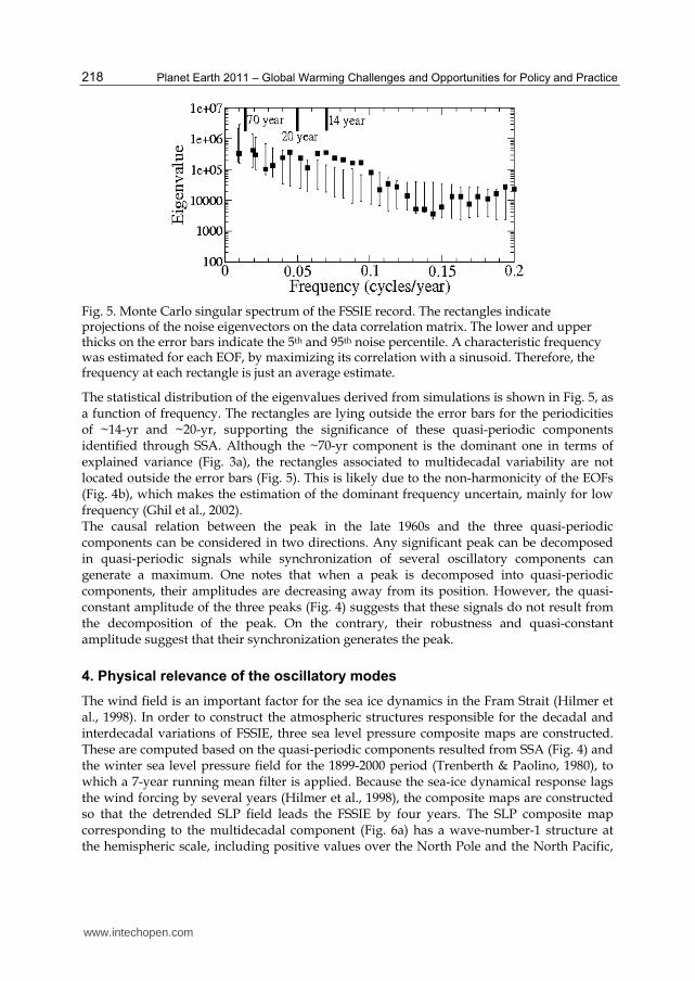
Fig. 5. Monte Carlo singular spectrum of the FSSIE record. The rectangles indicate projections of the noise eigenvectors on the data correlation matrix. The lower and upper thicks on the error bars indicate the 5th and 95th noise percentile. A characteristic frequency was estimated for each EOF, by maximizing its correlation with a sinusoid. Therefore, the frequency at each rectangle is just an average estimate.

The statistical distribution of the eigenvalues derived from simulations is shown in Fig. 5, as a function of frequency. The rectangles are lying outside the error bars for the periodicities of ~14-yr and ~20-yr, supporting the significance of these quasi-periodic components identified through SSA. Although the ~70-yr component is the dominant one in terms of explained variance (Fig. 3a), the rectangles associated to multidecadal variability are not located outside the error bars (Fig. 5). This is likely due to the non-harmonicity of the EOFs (Fig. 4b), which makes the estimation of the dominant frequency uncertain, mainly for low frequency (Ghil et al., 2002). The causal relation between the peak in the late 1960s and the three quasi-periodic components can be considered in two directions. Any significant peak can be decomposed in quasi-periodic signals while synchronization of several oscillatory components can generate a maximum. One notes that when a peak is decomposed into quasi-periodic components, their amplitudes are decreasing away from its position. However, the quasi-constant amplitude of the three peaks (Fig. 4) suggests that these signals do not result from the decomposition of the peak. On the contrary, their robustness and quasi-constant amplitude suggest that their synchronization generates the peak.

4. Physical relevance of the oscillatory modes

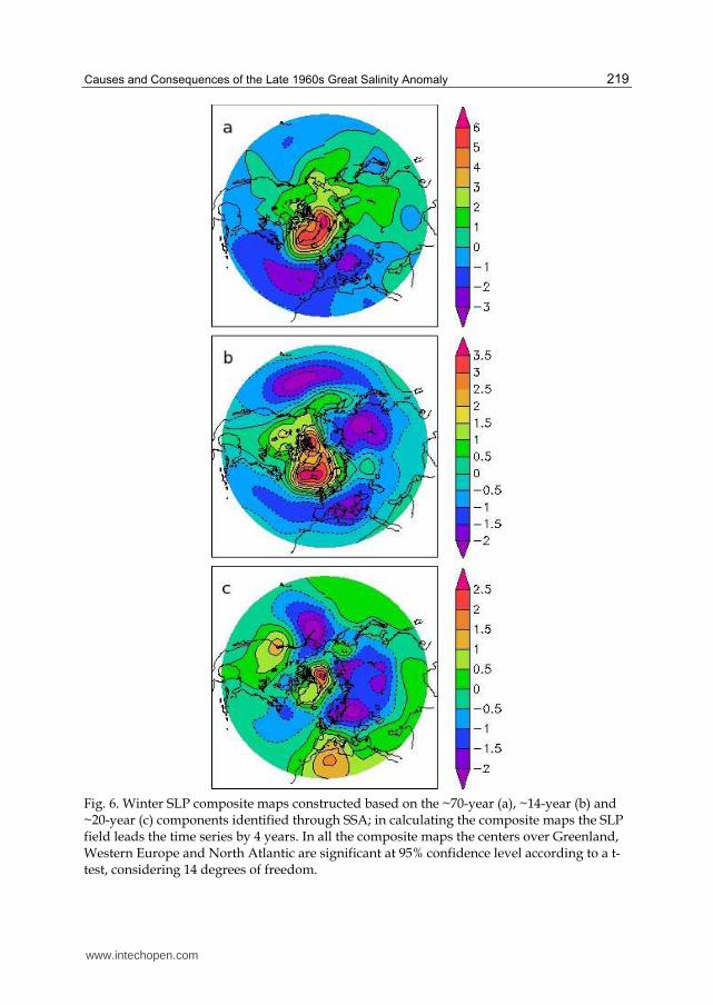
The wind field is an important factor for the sea ice dynamics in the Fram Strait (Hilmer et al., 1998). In order to construct the atmospheric structures responsible for the decadal and interdecadal variations of FSSIE, three sea level pressure composite maps are constructed. These are computed based on the quasi-periodic components resulted from SSA (Fig. 4) and the winter sea level pressure field for the 1899-2000 period (Trenberth & Paolino, 1980), to which a 7-year running mean filter is applied. Because the sea-ice dynamical response lags the wind forcing by several years (Hilmer et al., 1998), the composite maps are constructed so that the detrended SLP field leads the FSSIE by four years. The SLP composite map corresponding to the multidecadal component (Fig. 6a) has a wave-number-1 structure at the hemispheric scale, including positive values over the North Pole and the North Pacific,

www.intechopen.com


219

Fig. 6. Winter SLP composite maps constructed based on the ~70-year (a), ~14-year (b) and ~20-year (c) components identified through SSA; in calculating the composite maps the SLP field leads the time series by 4 years. In all the composite maps the centers over Greenland, Western Europe and North Atlantic are significant at 95% confidence level according to a t-test, considering 14 degrees of freedom.

www.intechopen.com


220

and negative values in the North Atlantic and over Europe. The highest values are concentrated in a high pressure system centered over Greenland. The associated wind field has a strong projection on FSSIE and contributes to an intensification of freshwater and sea ice export from the Arctic to the North Atlantic. This SLP structure was associated with the Atlantic Multidecadal Oscillation (Dima & Lohmann, 2007). The SLP composite map associated to the decadal mode (Fig. 6b) has an annular structure

with strong projection on the negative phase of the Arctic Oscillation (Thompson et al,

2000). The positive center extends over Greenland and the North Pole and favors

freshwater and sea ice export from the Arctic. A similar influence on the sea ice dynamics

is suggested by the SLP structure corresponding to the bidecadal mode (Fig. 6c), which

includes also a positive center over the North Pole. This SLP structure is similar to that

presented by White & Cayan (1998) in association with bidecadal variability (Figure 2 in

their study). One notes that the axis of maximum wind field from the Arctic toward the

North Atlantic for each SLP composite map aligns better with Fram Strait, as the mode

explains more variance in the FSSIE record (Fig. 6). Similarly, the SLP gradient across the

Fram Strait associated to each mode is higher, as the mode explains more variance in the

reconstruction. The composite maps show that the quasi-periodic decadal and

interdecadal variations identified in the FSSIE reconstruction are forced by specific

structures of atmospheric circulation.

In order to investigate possible associations between the quasi-periodic signals identified in

the FSSIE reconstruction and decadal modes of climate variability, correlation maps are

calculated between these time components and the sea surface temperature (SST) field from

the HADISST1 dataset (Rayner al., 2003). A maximum influence of a quasi-periodic climate

mode on FSSIE is generated for a specific phase of the modes. In general, this is different

from that phase of the mode which maximizes its influence on other fields, because different

physical processes could be involved. In order to consider these phase-shifts between

modes' projection on different fields, specific lags are considered when calculating

correlation maps, so that the obtained patters corresponds to the canonical SST structures of

these modes, presented in previous studies.

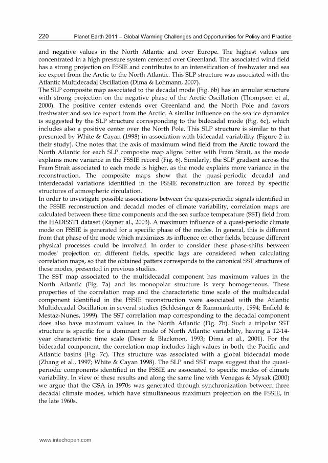
The SST map associated to the multidecadal component has maximum values in the

North Atlantic (Fig. 7a) and its monopolar structure is very homogeneous. These

properties of the correlation map and the characteristic time scale of the multidecadal

component identified in the FSSIE reconstruction were associated with the Atlantic

Multidecadal Oscillation in several studies (Schlesinger & Rammankutty, 1994; Enfield &

Mestaz-Nunes, 1999). The SST correlation map corresponding to the decadal component

does also have maximum values in the North Atlantic (Fig. 7b). Such a tripolar SST

structure is specific for a dominant mode of North Atlantic variability, having a 12-14-

year characteristic time scale (Deser & Blackmon, 1993; Dima et al., 2001). For the

bidecadal component, the correlation map includes high values in both, the Pacific and

Atlantic basins (Fig. 7c). This structure was associated with a global bidecadal mode

(Zhang et al., 1997; White & Cayan 1998). The SLP and SST maps suggest that the quasi-

periodic components identified in the FSSIE are associated to specific modes of climate

variability. In view of these results and along the same line with Venegas & Mysak (2000)

we argue that the GSA in 1970s was generated through synchronization between three

decadal climate modes, which have simultaneous maximum projection on the FSSIE, in

the late 1960s.

www.intechopen.com


221

Fig. 7. Correlation maps derived based on the SST field (Rayner et al., 2003) and the quasi-periodic signals obtained through SSA: a) the multidecadal (the component leads the field by 15-year), b) decadal (the component leads the field by 6-year), c) bidecadal (the component leads the field by 9-year). Before calculating the maps the warming trend was removed, by subtracting the annual global average from each grid point, and the SST field was filtered in the 10-17-year band (for the decadal component) and 17-26-year band (for the bidecadal component). For the multidecadal component a 21-year running mean filter was applied to the SST field.

www.intechopen.com


222

5. Possible consequences of the GSA

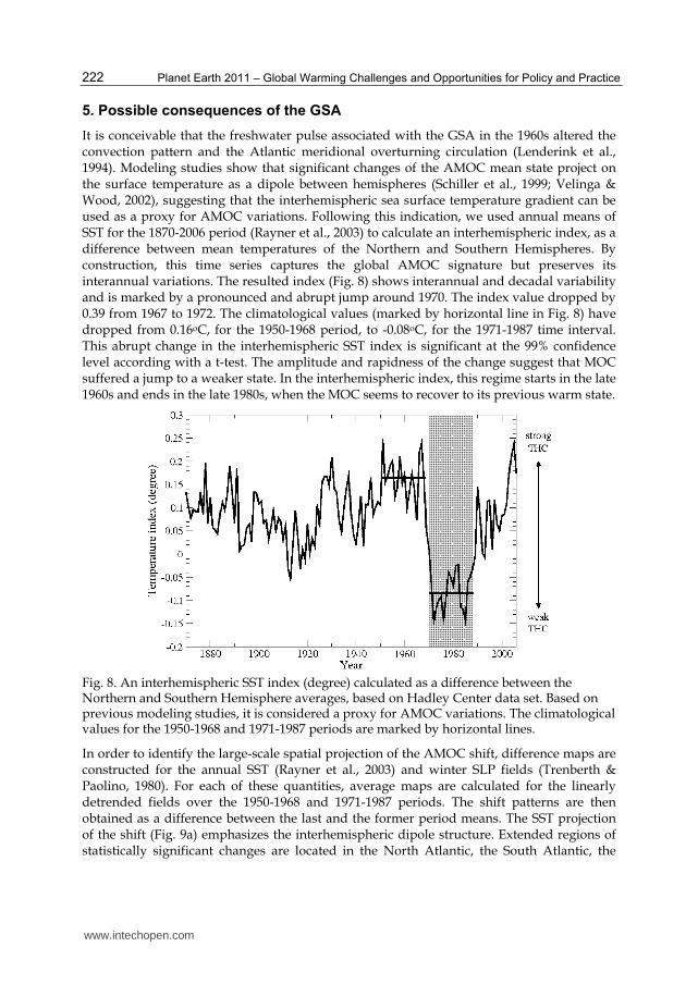
It is conceivable that the freshwater pulse associated with the GSA in the 1960s altered the convection pattern and the Atlantic meridional overturning circulation (Lenderink et al., 1994). Modeling studies show that significant changes of the AMOC mean state project on the surface temperature as a dipole between hemispheres (Schiller et al., 1999; Velinga & Wood, 2002), suggesting that the interhemispheric sea surface temperature gradient can be used as a proxy for AMOC variations. Following this indication, we used annual means of SST for the 1870-2006 period (Rayner et al., 2003) to calculate an interhemispheric index, as a difference between mean temperatures of the Northern and Southern Hemispheres. By construction, this time series captures the global AMOC signature but preserves its interannual variations. The resulted index (Fig. 8) shows interannual and decadal variability and is marked by a pronounced and abrupt jump around 1970. The index value dropped by 0.39 from 1967 to 1972. The climatological values (marked by horizontal line in Fig. 8) have dropped from 0.16oC, for the 1950-1968 period, to -0.08oC, for the 1971-1987 time interval. This abrupt change in the interhemispheric SST index is significant at the 99% confidence level according with a t-test. The amplitude and rapidness of the change suggest that MOC suffered a jump to a weaker state. In the interhemispheric index, this regime starts in the late 1960s and ends in the late 1980s, when the MOC seems to recover to its previous warm state.

Fig. 8. An interhemispheric SST index (degree) calculated as a difference between the Northern and Southern Hemisphere averages, based on Hadley Center data set. Based on previous modeling studies, it is considered a proxy for AMOC variations. The climatological values for the 1950-1968 and 1971-1987 periods are marked by horizontal lines.

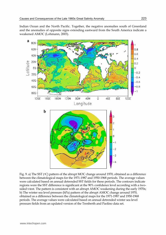
In order to identify the large-scale spatial projection of the AMOC shift, difference maps are constructed for the annual SST (Rayner et al., 2003) and winter SLP fields (Trenberth & Paolino, 1980). For each of these quantities, average maps are calculated for the linearly detrended fields over the 1950-1968 and 1971-1987 periods. The shift patterns are then obtained as a difference between the last and the former period means. The SST projection of the shift (Fig. 9a) emphasizes the interhemispheric dipole structure. Extended regions of statistically significant changes are located in the North Atlantic, the South Atlantic, the

www.intechopen.com


223

Indian Ocean and the North Pacific. Together, the negative anomalies south of Greenland and the anomalies of opposite signs extending eastward from the South America indicate a weakened AMOC (Lohmann, 2003).

Fig. 9. a) The SST (oC) pattern of the abrupt MOC change around 1970, obtained as a difference between the climatological maps for the 1971-1987 and 1950-1968 periods. The average values were calculated based on annual detrended SST fields for these periods. The contours indicate regions were the SST difference is significant at the 90% confidence level according with a two-sided t-test. The pattern is consistent with an abrupt AMOC weakening during the early 1970s; b) The winter sea level pressure (hPa) pattern of the abrupt AMOC change around 1970, obtained as a difference between the climatological maps for the 1971-1987 and 1950-1968 periods. The average values were calculated based on annual detrended winter sea level pressure fields from an updated version of the Trenberth and Paolino data set.

www.intechopen.com


224

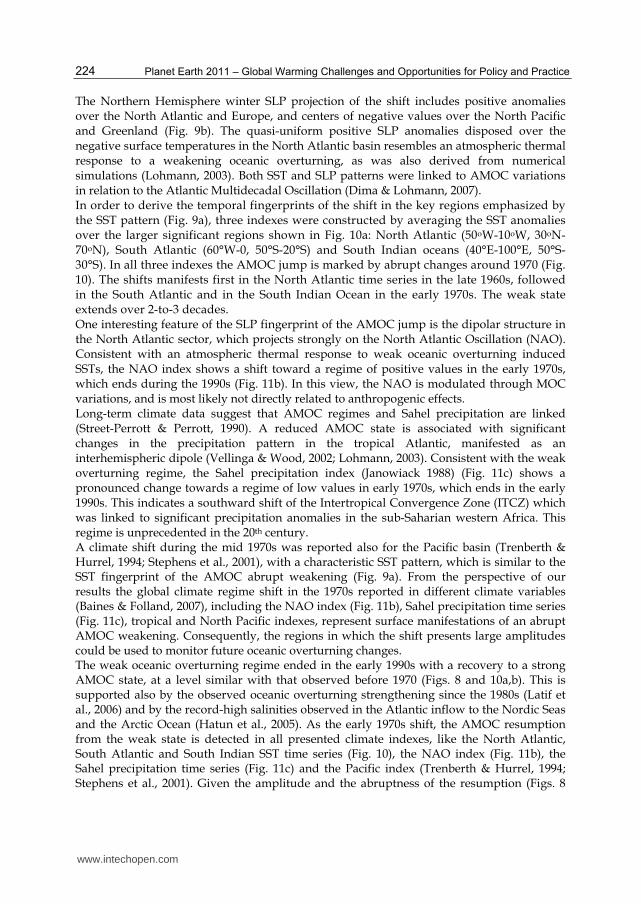
The Northern Hemisphere winter SLP projection of the shift includes positive anomalies over the North Atlantic and Europe, and centers of negative values over the North Pacific and Greenland (Fig. 9b). The quasi-uniform positive SLP anomalies disposed over the negative surface temperatures in the North Atlantic basin resembles an atmospheric thermal response to a weakening oceanic overturning, as was also derived from numerical simulations (Lohmann, 2003). Both SST and SLP patterns were linked to AMOC variations in relation to the Atlantic Multidecadal Oscillation (Dima & Lohmann, 2007). In order to derive the temporal fingerprints of the shift in the key regions emphasized by the SST pattern (Fig. 9a), three indexes were constructed by averaging the SST anomalies over the larger significant regions shown in Fig. 10a: North Atlantic (50oW-10oW, 30oN-70oN), South Atlantic (60°W-0, 50°S-20°S) and South Indian oceans (40°E-100°E, 50°S-30°S). In all three indexes the AMOC jump is marked by abrupt changes around 1970 (Fig. 10). The shifts manifests first in the North Atlantic time series in the late 1960s, followed in the South Atlantic and in the South Indian Ocean in the early 1970s. The weak state extends over 2-to-3 decades. One interesting feature of the SLP fingerprint of the AMOC jump is the dipolar structure in the North Atlantic sector, which projects strongly on the North Atlantic Oscillation (NAO). Consistent with an atmospheric thermal response to weak oceanic overturning induced SSTs, the NAO index shows a shift toward a regime of positive values in the early 1970s, which ends during the 1990s (Fig. 11b). In this view, the NAO is modulated through MOC variations, and is most likely not directly related to anthropogenic effects. Long-term climate data suggest that AMOC regimes and Sahel precipitation are linked (Street-Perrott & Perrott, 1990). A reduced AMOC state is associated with significant changes in the precipitation pattern in the tropical Atlantic, manifested as an interhemispheric dipole (Vellinga & Wood, 2002; Lohmann, 2003). Consistent with the weak overturning regime, the Sahel precipitation index (Janowiack 1988) (Fig. 11c) shows a pronounced change towards a regime of low values in early 1970s, which ends in the early 1990s. This indicates a southward shift of the Intertropical Convergence Zone (ITCZ) which was linked to significant precipitation anomalies in the sub-Saharian western Africa. This regime is unprecedented in the 20th century. A climate shift during the mid 1970s was reported also for the Pacific basin (Trenberth & Hurrel, 1994; Stephens et al., 2001), with a characteristic SST pattern, which is similar to the SST fingerprint of the AMOC abrupt weakening (Fig. 9a). From the perspective of our results the global climate regime shift in the 1970s reported in different climate variables (Baines & Folland, 2007), including the NAO index (Fig. 11b), Sahel precipitation time series (Fig. 11c), tropical and North Pacific indexes, represent surface manifestations of an abrupt AMOC weakening. Consequently, the regions in which the shift presents large amplitudes could be used to monitor future oceanic overturning changes. The weak oceanic overturning regime ended in the early 1990s with a recovery to a strong AMOC state, at a level similar with that observed before 1970 (Figs. 8 and 10a,b). This is supported also by the observed oceanic overturning strengthening since the 1980s (Latif et al., 2006) and by the record-high salinities observed in the Atlantic inflow to the Nordic Seas and the Arctic Ocean (Hatun et al., 2005). As the early 1970s shift, the AMOC resumption from the weak state is detected in all presented climate indexes, like the North Atlantic, South Atlantic and South Indian SST time series (Fig. 10), the NAO index (Fig. 11b), the Sahel precipitation time series (Fig. 11c) and the Pacific index (Trenberth & Hurrel, 1994; Stephens et al., 2001). Given the amplitude and the abruptness of the resumption (Figs. 8

www.intechopen.com


225

and 10a,b) in the early 1990s, one can consider that a climate regime shift, associated with a rapid strengthening of Atlantic meridional overturning, was experienced in the last decade.

Fig. 10. SST indexes (degree) derived as averages over the a) North Atlantic (50°W-10°W, 30°N-70°N); b) South Atlantic (60°W-0, 50°S-20°S); c) South Indian oceans (40°E-100°E, 50°S-30°S). All three indexes emphasize an AMOC jump to a weaker state during 1970s.

www.intechopen.com


226

Fig. 11. a) Normalized Fram Strait Sea Ice Export for the 1899-2000 period; b) Principal Component based December-January-February-March average North Atlantic Oscillation index for the 1899-2006 period; the PC analysis was performed on the SLP field over the Atlantic sector (20°-80°N, 90°W-40°E); c) Normalized Sahel precipitation index for the 1898-2004 period

www.intechopen.com


227

Due to its prominence and spreading path along east Greenland, the GSA in the 1960s represented a significant forcing reaching the Labrador Sea convection region (Dickson et al., 1988). It was the first event from a series of several significant salinity anomalies with decreasing amplitudes, which ended in the late 1980s. Anomalous strong sea-ice export from the Arctic through Fram Strait (Fig. 11a), as that associated with the GSAs (Schmith & Hansen, 2003), would increase the fresh water fluxes in the North Atlantic (Hilmer et al., 1998) and can modulate the AMOC (Häkkinen, 1999). Numerical experiments show that a fresh water pulse applied in the North Atlantic can generate an AMOC shift on a weak state, which is manifested at the surface as a center of pronounced negative anomalies south of Greenland (Rahmstorf, 1994), as seen in Fig. 9a. A similar fingerprint on the surface temperature was attributed to a weakening oceanic overturning in response to a freshwater pulse associated with the 8.2-kyr event (Renssen et al., 2002). For preindustrial climate the SST and SLP response patterns to an AMOC collapse are similar to the corresponding patterns of the 1970s shift, although with a larger amplitude (Vellinga & Wood, 2002) (Fig. 9a,b). A multi model ensemble of numerical experiments related to the ocean response to fresh water forcing reproduces well the general features of the SST pattern of the shift (Fig. 9a) and accurately the dipole anomaly pattern in North Atlantic, which includes cooling south of Greenland and warming over the Barents and Nordic Seas (Stouffer et al., 2006). It is conceivable that the freshwater pulse associated with the GSA in the 1960s altered the convection pattern and the AMOC (Lenderink & Haarsma, 1994). The changed convection pattern is possibly responsible for the jump to a weaker state. According to model simulations (Lohmann, 2003), the associated ~1.5°C change in SST can be translated to a moderate AMOC reduction of 10%-20%. This results in a freshening of the North Atlantic surface layers in the last decades (Dickson et al., 2002; Curry & Mauritzen, 2005). The AMOC attends the new weak state several years after the GSA in the late 1960s, consistent with a fast response of the meridional overturning to North Atlantic forcing (Eden & Willebrand, 2001). From this perspective, the 1960s GSA represents the cause for the AMOC jump to a new weaker state around 1970. The significant fresh water forcing related to Fram Strait Sea Ice Export starts in the late 1960s and ends in the late 1980s (Fig. 11a), while the weak state extends from the early 1970s to the early 1990s (Figs. 8 and 10a). It appears therefore that the AMOC responded in a direct way to the forcing so that the weak state persisted as long as the anomalous forcing acted.

6. Summary and conclusions

Following the hypothesis that the GSA in the late 1960s has an Arctic origin, the SSA method is applied to identify the quasi-periodic components in the FSSIE reconstruction (Schmith & Hansen, 2003). The analysis emphasizes that the maximum in the late 1960s in the FSSIE record resulted from a synchronization between time-components with periods of ~70-yr, ~14-yr and ~20-yr, consistent with a previous study based on a shorter data set (Venegas & Mysak, 2000). The statistical significance of time-components was tested with Monte Carlo simulations. The time components are associated with known climate cycles (Enfield & Mestaz-Nunes, 1999; Deser & Blackmon, 1993; White & Cayan, 1998), suggesting that modes synchronization can represent an important deterministic mechanism for generating large-scale climate anomalies. In view of the restricted number of analyzed fields and time series, and their limited time extension, more investigations based on different data sets are necessary in order to validate these results.

www.intechopen.com


228

As we suggest that the late 1960s GSA was caused by synchronization between three climatic modes, one may speculate that the ~70-years, ~14-years and ~20-years periods of the climate modes, which synchronized in the late 1960s, point to a ~140-yr recurrence time of the GSA. Accordingly, a similar synchronization is observed in 1830s (Fig. 4c) and the next one is anticipated for the 2110s, if the cycles continue to exist. An interesting point concerns a possible factors of the anthropogenic influences on the GSA. The quasi-periodic nature of the synchronized time-components which generate the GSA excludes a potential anthropogenic origin of this freshwater anomaly because this evolves in time as a trend. However, the anthropogenic factor could provide a relatively warm background on which the amplitude and impact of a potential future GSA can be much larger. Using information derived from numerical experiments we synthesize a large amount of observational data and increase the signal-to-noise ratio related to AMOC changes. Based on an inter-hemispheric and on regional indexes we present evidence and argue that the freshwater pulse associated with the late 1960s GSA modified the convection pattern in the northern North Atlantic, generating an abrupt AMOC weakening, which manifested at the surface as a climate regime shift. This weak state lasted 2 to 3 decades and ended in the early 1990s, with a rapid resumption of the AMOC on a strong state. Our study demonstrates the possibility of monitoring large-scale oceanic changes using observational data and points to key surface locations on which such variations have optimal projections. The identification of abrupt AMOC changes over the modern period and its association with climate regime shifts suggest that future rapid climate changes are also likely in a globally warming world. The fact that an abrupt but moderate MOC reduction caused a climate regime shift in surface variables points to a larger climatic impact generated by possibly more significant AMOC changes. It was shown based on numerical experiments that prominent climatic events can be generated in the climate system without variable external forcing (Hall & Stouffer, 2001). Our results based on observational and reconstructed data show that a significant climate anomaly, like GSA, can be generated without need of anomalous external forcing, but just through a constructive interference of quasi-periodic time-components. Consequently, the climate shift in the 1970s appears as a result of a resonance between several climate modes.

7. References

Aagard, K. & Carmack, E. C. (1989). The role of sea ice and other freshwater in the Arctic circulation, Journal of Geophysical Research, Vol.94, pp. 305-311.

Allen, M. & Smith, L. A. (1997). Optimal filtering in Singular Spectrum Analysis, Physical Letters, Vol.234, pp.419-428.

Alley, R. B.; Anandakrishman, S. & Jung, P. (2001). Stochastic resonance in the North Atlantic, Paleoceanography, Vol.16, pp. 190-198.

Baines, P. G., & Folland, C. K. (2007). Evidence for a Rapid Global Climate Shift across the Late 1960s, Journal of Climate, Vol.20, pp. 2721-2744.

Barber, D. C.; Dyke, A; Hillaire-Marcel, C.; Jennings, A. E.; Andrews, J. T.; Kerwin, M. W.; Bilodeau, G;, McNeely, R.; Southon, J.; Morehead, M. D. & Gagnon, J. M. (1999). Forcing of the cold event of 8,200 years ago by catastrophic drainage of Laurentide lakes, Nature, Vol.400, pp. 344-348.

Cavalieri, D. J. (2002). A Link Between Fram Strait sea ice export and atmospheric planetary wave phase, Geophysical Research Letters, Vol.29, No.12, pp. 56-1 – 56-4.

www.intechopen.com


229

Curry, R., & Mauritzen, C. (2005). Dilution of the Northern North Atlantic Ocean in Recent Decades, Science, Vol.308, pp. 1772-1774.

Dansgaard, W.; Johnsen, S. J.; Clausen, H. B.; Dahl-Jensen, D.; Gundestrup, N. S.; Hammer, C. U.; Hvidberg, C. S.; Steffensen, J. P.; Sveinbjomsdottir, A. E.; Jouzel, J. & Bond, G. (1993). Evidence for general instability of past climate from a 250-kyr ice-core record, Nature, Vol.364, pp. 218-220.

Deser, C. & Blackmon, M. L. (1993). Surface Climate Variations over the North Atlantic Ocean during Winter: 1900-1989, Journal of Climate, Vol.6, pp. 1743-1753.

Dickson, R. R.; Meinecke, J.; Malmberg, S.-A. & Lee, A. J. (1988). The "great salinity anomaly" in the northern North Atlantic 1968-1982, Progress in Oceanography, Vol.20, pp. 103-151.

Dickson, R.R.; Yashayev, I.; Meincke, J.; Turrell, W.; Dye, S. & Holfort, J. (2002). Rapid freshening of the deep North Atlantic Ocean over the past four decades, Nature, Vol.416, pp. 832-837.

Dima, M; Rimbu, N.; Stefan, S. & Dima, I. (2001). Quasi-Decadal Variability in the Atlantic Basin involving Tropics-Midlatitudes and Ocean-Atmosphere Interactions, Journal of Climate, Vol.14, pp. 823-832.

Dima, M. & Lohmann, G. (2007). A Hemispheric Mechanism for the Atlantic Multidecadal Oscillation, Journal of Climate, Vol.20, pp. 2706-2719.

Eden, C., & Willebrand, J. (2001). Mechanism of Interannual to Decadal Variability of the North Atlantic Circulation, Journal of Climate, Vol.14, pp. 2266-2280.

Enfield, D. B. & Mestas-Nunes, A. M. (1999). Multiscale variabilities in global sea surface temperatures and their relationship with tropospheric climate patterns, Journal of Climate, Vol.12, pp. 2719-2733.

EPICA Community Members (2006). One-to-one coupling of glacial climate variability in Greenland and Antarctica, Nature, Vol.444, pp. 195-198.

Ghil, M.; Allen, M. R.; Dettinger, M. D.; Ide, K.; Kondrashov, D.; Mann, M. E.; Robertson, A. W.; Saunders, A.; Tian, Y.; Varadi, F. & Yiou, P. (2002). Advanced spectral methods for climatic time series, Reviews of Geophysics, 8755-1209/02/2000RG000092, 1-1-1-41.

Hall, A., & Stouffer, R. J. (2001). An abrupt climate event in a coupled ocean-atmosphere simulation without external forcing, Nature, Vol.409, pp. 171-174.

Hatun, H., Sande, A. B., Drange, H., Hansen, B. & Valdimarsson, H. Influence of the Atlantic Subpolar Gyre on the Thermohaline Circulation, Science, 309, 1841-1844 (2005).

Häkkinen, S. (1999). A simulation of thermohaline effects of a Great Salinity. Anomaly, Journal of Climate, Vol.12, pp. 1781-1795.

Häkkinen, H. & Geiger, C. A. (2002). Simulated low-frequency modes of circulation in the Arctic, Journal of Geophysical Research, Vol.105, No.C3, pp. 6549-6564.

Heinrich, H. (1988). Origin and consequence of cyclic ice rafting in the northeast Atlantic Ocean during the past 130,000 years, Quaternary Research, Vol.29, pp. 3359-3362.

Hilmer, R.; Harder, M. & Lemke, P. (1998). Sea ice transport: A highly variable link between Arctic and North Atlantic, Geophysical Research Letters, Vol.25, pp. 3359-3362.

Janowiak, J. E. (1988). An investigation of interannual rainfall variability in Africa, Journal of Climate, Vol.1, pp. 240-255.

Latif, M. et al. (2006). Is the Thermohaline Circulation Changing ?, Journal of Climate, Vol.19, pp. 4631-4637.

www.intechopen.com


230

Lenderink, G. & Haarsma, H. (1994). Variability and multiple equilibria of the thermohaline circulation associated with deep water fromation, Journal of Physical Oceanography, Vol.24, pp. 1480-1493.

Lohmann, G. (2003). Atmospheric and oceanic freshwater transport during weak Atlantic overturning circulation, Tellus, Vol.55, pp. 439-448.

Rahmstorf, S. (1994) Rapid climate transitions in a coupled ocean-atmosphere model, Nature, Vol.372, pp. 82-85.

Rayner, N. A. et al. (2003). Global analyses of sea surface temperature, sea ice, and night marine air temperature since the late nineteenth century, Journal of Geophysical Research, Vol.108, 10.1029/2002JD002670.

Renssen, H.; Goosse, H. & Fichelet, T. (2002). Modeling the effect of freshwater pulses on the early Holocene climate: the influence of high-frequency climate variability, Paleoceanography, Vol.17, No.2, 1020, DOI: 10.1029/2001PA000649.

Schiller, A.; Mikolajewicz, U. & Voss, R. (1997). The stability of the North Atlantic thermohaline circulation in a coupled ocean-atmosphere general circulation model. Climate Dynamics, Vol.13, pp. 325-347.

Schlesinger, M. E. & Ramankutty, N. (1994). An oscillation in the global climate system of period 65-70 years, Nature, Vol.367, pp. 723-726.

Schmith, T. & Hansen, C. (2003). Fram Strait ice export during the nineteenth and twentieth centuries reconstructed from a multiyear sea ice index from Southwestern Greenland, Journal of Climate, Vol.16, pp. 2782-2792.

Stephens, C., Levitus, S., Antonov, J. & Boyer, T. P. (2001). On the Pacific Ocean regime shift, Geophysical Research Letters, Vol.28, No.19, pp. 3721-3724.

Stommel, H. (1961). Thermohaline convection with two stable regimes of flow, Tellus, Vol.13, pp. 2782-2792.

Stouffer, R. J. et al. (2006). Investigating the Causes and Response of the Thermohaline Circulation to Past and Future Climate Changes, Journal of Climate, Vol.19, pp. 1365-1387.

Thompson, D. W. J.; Wallace, J. M. & Hegerl, G. C. (2000). Annular modes in the extratropical circulation. Part II: Trends, Journal of Climate, Vol.13, pp. 1018-1036.

Trenberth, K. A. & Paolino, D. A. (1980). The Northern Hemisphere sea-level pressure, Monthly Weather Review, Vol.108, pp. 855-872.

Vellinga, M. & Wood, R. A. (2002). Global climatic impacts of a collapse of the Atlantic thermohaline circulation, Climate Change, Vol. 54, pp. 251-267.

Venegas, S. A. & Mysak, L. A. (2000). Is there a Dominant Timescale of Natural Climate Variability in the Arctic?, Journal of Climate, Vol.13, pp. 3412-3434.

White, W. B. & Cayan, D. R. (1998). Quasi-periodicity and global symmetries in interdecadal upper ocean temperature variability, Journal of Geophysical Research, Vol.103, pp. 21335-21354.

Zhang, Y.; Wallace, J. M. & Battisti, D. S. (1997). ENSO-like interdecadal variability: 1900-1993, Journal of Climate, Vol.10, pp. 1004-1020.

www.intechopen.com

Planet Earth 2011 - Global Warming Challenges and Opportunitiesfor Policy and PracticeEdited by Prof. Elias Carayannis

ISBN 978-953-307-733-8Hard cover, 646 pagesPublisher InTechPublished online 30, September, 2011Published in print edition September, 2011

InTech EuropeUniversity Campus STeP Ri Slavka Krautzeka 83/A 51000 Rijeka, Croatia Phone: +385 (51) 770 447 Fax: +385 (51) 686 166www.intechopen.com

InTech ChinaUnit 405, Office Block, Hotel Equatorial Shanghai No.65, Yan An Road (West), Shanghai, 200040, China

Phone: +86-21-62489820 Fax: +86-21-62489821

The failure of the UN climate change summit in Copenhagen in December 2009 to effectively reach a globalagreement on emission reduction targets, led many within the developing world to view this as a reversal ofthe Kyoto Protocol and an attempt by the developed nations to shirk out of their responsibility for climatechange. The issue of global warming has been at the top of the political agenda for a number of years and hasbecome even more pressing with the rapid industrialization taking place in China and India. This book looks atthe effects of climate change throughout different regions of the world and discusses to what extent cleantechand environmental initiatives such as the destruction of fluorinated greenhouse gases, biofuels, and the role ofplant breeding and biotechnology. The book concludes with an insight into the socio-religious impact thatglobal warming has, citing Christianity and Islam.

How to referenceIn order to correctly reference this scholarly work, feel free to copy and paste the following:

Mihai Dima and Gerrit Lohmann (2011). Causes and Consequences of the Late 1960s Great Salinity Anomaly,Planet Earth 2011 - Global Warming Challenges and Opportunities for Policy and Practice, Prof. EliasCarayannis (Ed.), ISBN: 978-953-307-733-8, InTech, Available from: http://www.intechopen.com/books/planet-earth-2011-global-warming-challenges-and-opportunities-for-policy-and-practice/causes-and-consequences-of-the-late-1960s-great-salinity-anomaly

causes and consequences of the late 1960s great salinity ... · causes and consequences of the late...

Documents