causes and counterfactuals: concepts, principles and...
TRANSCRIPT

CAUSES AND COUNTERFACTUALS:
CONCEPTS, PRINCIPLES AND TOOLS
Judea Pearl Elias Bareinboim
University of California, Los Angeles {judea, eb}@cs.ucla.edu
NIPS 2013 Tutorial
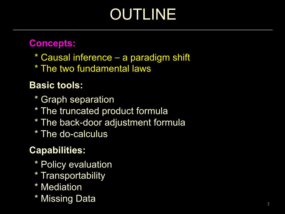
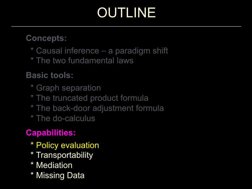
OUTLINE!
Concepts:
* Causal inference ⎯ a paradigm shift * The two fundamental laws
Basic tools:
* Graph separation * The truncated product formula * The back-door adjustment formula * The do-calculus
Capabilities:
* Policy evaluation * Transportability * Mediation * Missing Data!
2
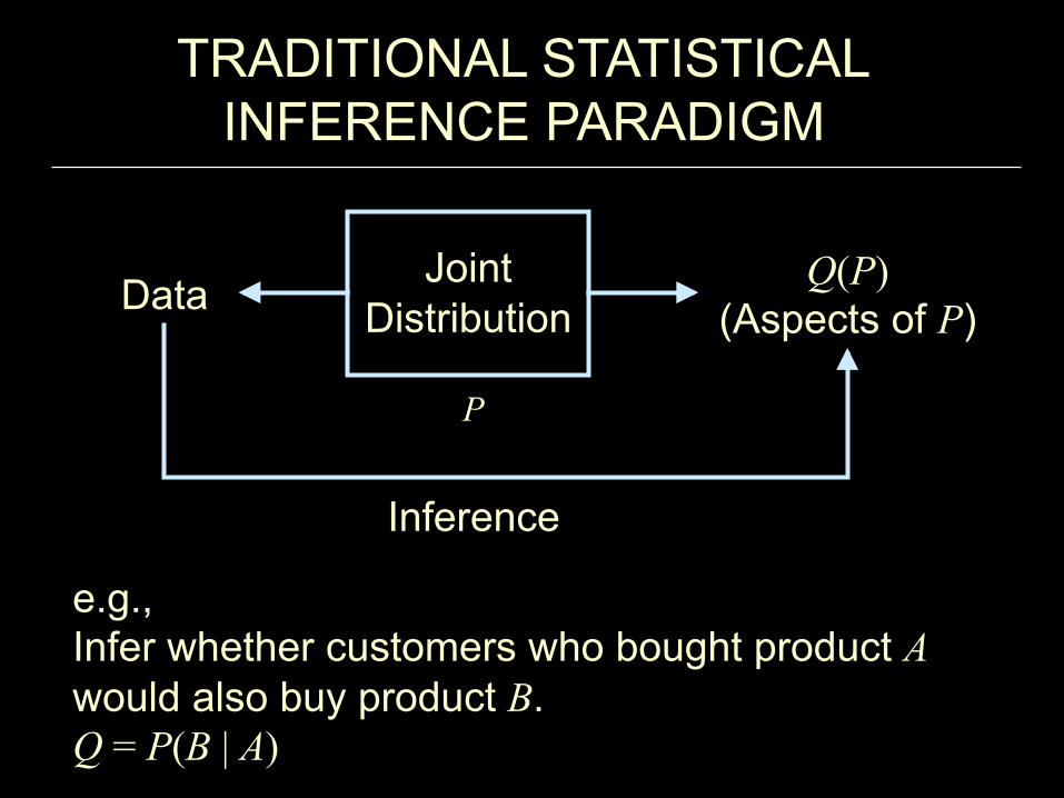
TRADITIONAL STATISTICAL INFERENCE PARADIGM
Data
Inference
Q(P) (Aspects of P)
e.g., Infer whether customers who bought product A would also buy product B. Q = P(B | A)
Joint Distribution
P

e.g., Estimate P′(sales) if we double the price. How does P change to P′? New oracle e.g., Estimate P′(cancer) if we ban smoking.
FROM STATISTICAL TO CAUSAL ANALYSIS: 1. THE DIFFERENCES
Data
Inference
Q(P′) (Aspects of P′)
change
Joint Distribution
P
Joint Distribution
P′

What remains invariant when P changes say, to satisfy P′(price=2)=1
Data
Inference
Q(P′) (Aspects of P′)
change
Note: P′(sales) ≠ P (sales | price = 2)
e.g., Doubling price ≠ seeing the price doubled.
P does not tell us how it ought to change.
FROM STATISTICAL TO CAUSAL ANALYSIS: 1. THE DIFFERENCES
Joint Distribution
P
Joint Distribution
P′
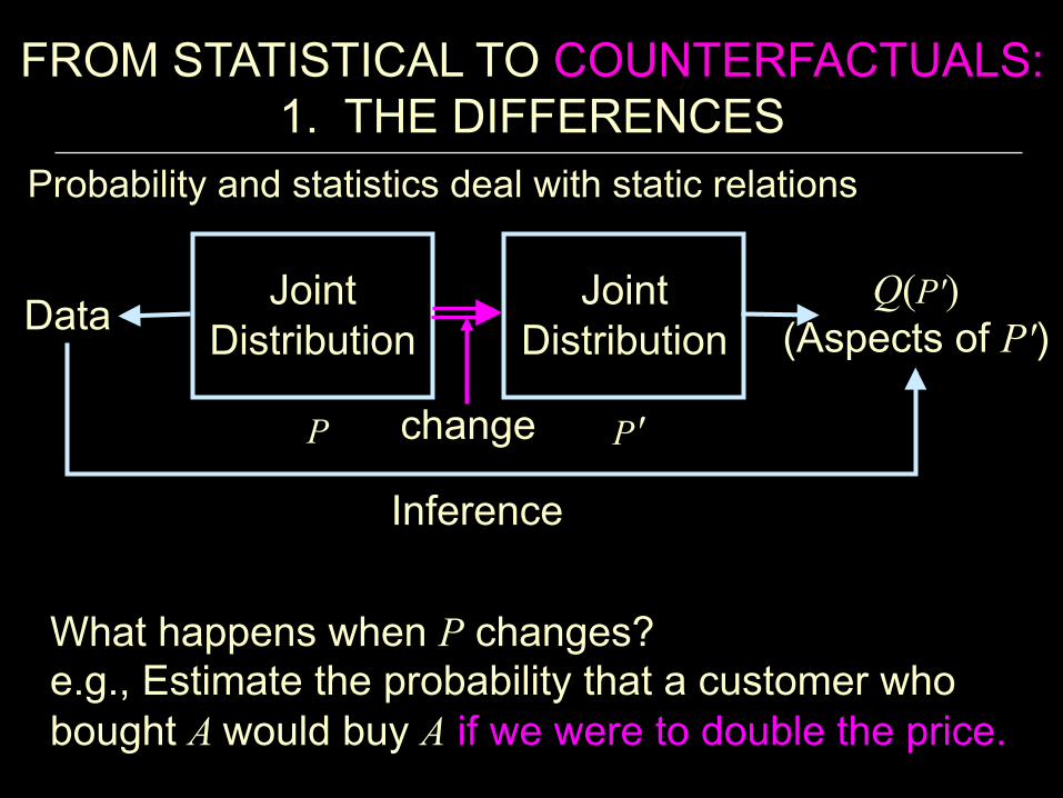
What happens when P changes? e.g., Estimate the probability that a customer who bought A would buy A if we were to double the price.
FROM STATISTICAL TO COUNTERFACTUALS: 1. THE DIFFERENCES
Probability and statistics deal with static relations
Data
Inference
Q(P′) (Aspects of P′)
change
Joint Distribution
P
Joint Distribution
P′

Data
Inference
Q(M) (Aspects of M)
Data Generating
Model
M – Invariant strategy (mechanism, recipe, law, protocol) by which Nature assigns values to variables in the analysis.
Joint Distribution
THE STRUCTURAL MODEL PARADIGM
M
P – model of data, M – model of reality •
P
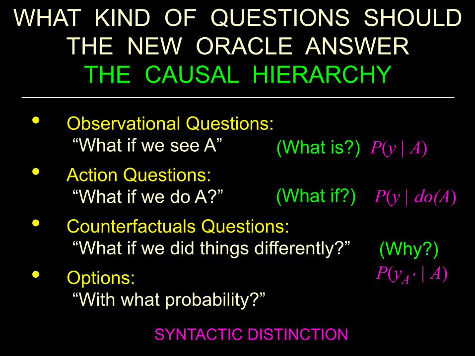
WHAT KIND OF QUESTIONS SHOULD THE NEW ORACLE ANSWER
THE CAUSAL HIERARCHY
(What is?)
(What if?)
(Why?)
P(y | A)
P(y | do(A)
P(yA’ | A)
SYNTACTIC DISTINCTION
• Observational Questions: “What if we see A”
• Action Questions: “What if we do A?”
• Counterfactuals Questions: “What if we did things differently?”
• Options: “With what probability?”

WHAT KIND OF QUESTIONS SHOULD THE NEW ORACLE ANSWER
THE CAUSAL HIERARCHY
• Observational Questions: “What if we see A”
• Action Questions: “What if we do A?”
• Counterfactuals Questions: “What if we did things differently?”
• Options: “With what probability?”
Bayes Networks
Causal Bayes Networks
Functional Causal Diagrams
GRAPHICAL REPRESENTATIONS

FROM STATISTICAL TO CAUSAL ANALYSIS: 2. THE SHARP BOUNDARY
CAUSAL Spurious correlation Randomization / Intervention “Holding constant” / “Fixing” Confounding / Effect Instrumental variable Ignorability / Exogeneity
ASSOCIATIONAL Regression Association / Independence “Controlling for” / Conditioning Odds and risk ratios Collapsibility / Granger causality Propensity score
1. Causal and associational concepts do not mix.
2.
3.
4.

4. Non-standard mathematics: a) Structural equation models (Wright, 1920; Simon, 1960) b) Counterfactuals (Neyman-Rubin (Yx), Lewis (x Y))
ASSOCIATIONAL Regression Association / Independence “Controlling for” / Conditioning Odds and risk ratios Collapsibility / Granger causality Propensity score
1. Causal and associational concepts do not mix.
3. Causal assumptions cannot be expressed in the mathematical language of standard statistics.
FROM STATISTICAL TO CAUSAL ANALYSIS: 3. THE MENTAL BARRIERS
2. No causes in – no causes out (Cartwright, 1989)
causal conclusions ⇒ } data causal assumptions (or experiments)
CAUSAL Spurious correlation Randomization / Intervention “Holding constant” / “Fixing” Confounding / Effect Instrumental variable Ignorability / Exogeneity

THE NEW ORACLE: STRUCTURAL CAUSAL MODELS
THE WORLD AS A COLLECTION OF SPRINGS
Definition: A structural causal model is a 4-tuple <V,U, F, P(u)>, where • V = {V1,...,Vn} are endogenous variables • U = {U1,...,Um} are background variables • F = {f1,..., fn} are functions determining V,
vi = fi(v, u)
• P(u) is a distribution over U
P(u) and F induce a distribution P(v) over observable variables
y = α +βx + uYe.g., Not regression!!!!

Definition: Given a SCM model M, the potential outcome Yx(u) for unit u is equal to the solution for Y in a mutilated model Mx, in which the equation for X is replaced by X = x.
The Fundamental Equation of Counterfactuals:
COUNTERFACTUALS ARE EMBARRASSINGLY SIMPLE
U
X (u) Y (u)
M U
X = x Yx (u)
Mx
Yx (u) Δ= YMx (u)

Definition: Given a SCM model M, the effect of setting X to x, P(Y = y | do (X=x)), is equal to the probability of Y = y in a mutilated model Mx, in which the equation for X is replaced by X = x.
The Fundamental Equation of Interventions:
EFFECTS OF INTERVENTIONS ARE EMBARRASSINGLY SIMPLE
U
X (u) Y (u)
M U
X = x Yx (u)
Mx
P(Y = y | do(X = x)) Δ= PMx (Y = y) = P(Yx = y)

P(x, y,u) = P(u)P(x | u)P(y | x,u)
The Fundamental Equation of Interventions:
COMPUTING THE EFFECTS OF INTERVENTIONS
U
X (u) Y (u)
M U
X = x Yx (u)
Mx
P(Y = y | do(X = x)) Δ= PMx (Y = y)
P(y,u | do(x)) = P(u)P(y | x,u)
P(y | do(x)) = P(y | x,u)P(u)u∑
Truncated product
Adjustment formula

THE TWO FUNDAMENTAL LAWS OF CAUSAL INFERENCE
1. The Law of Counterfactuals (and Interventions) (M generates and evaluates all counterfactuals.)
2. The Law of Conditional Independence (d-separation) (Separation in the model ⇒ independence in the distribution.)
Yx (u) = YMx (u)
(X sep Y | Z )G(M )⇒ (X ⊥⊥ Y | Z )P(v)

Gift of the Gods
If the U 's are independent, the observed distribution P(C,R,S,W) satisfies constraints that are: (1) independent of the f 's and of P(U), (2) readable from the graph.
C (Climate)
R (Rain)
S (Sprinkler)
W (Wetness)
THE LAW OF CONDITIONAL INDEPENDENCE
C = fC (UC )S = fS (C,US )R = fR(C,UR )W = fW (S,R,UW )
Graph (G) Model (M)

D-SEPARATION: NATURE’S LANGUAGE FOR COMMUNICATING ITS STRUCTURE
C (Climate)
R (Rain)
S (Sprinkler)
W (Wetness) Every missing arrow advertises an independency, conditional on a separating set.
Applications: 1. Model testing 2. Structure learning 3. Reducing "what if I do" questions to symbolic calculus 4. Reducing scientific questions to symbolic calculus
C = fC (UC )S = fS (C,US )R = fR(C,UR )W = fW (S,R,UW )
e.g., C ⊥⊥ W | (S,R) S ⊥⊥ R |C
Graph (G) Model (M)

OUTLINE!
Concepts:
* Causal inference ⎯ a paradigm shift * The two fundamental laws
Basic tools:
* Graph separation * The truncated product formula * The back-door adjustment formula * The do-calculus
Capabilities:
* Policy evaluation * Transportability * Mediation * Missing Data!

FIRST LAYER OF THE CAUSAL HIERARCHY
PROBABILITIES (What if I see X=x?)!

Data!
Data Generating
Model!
Joint Distribution
!
THE EMERGENCE OF THE FIRST LAYER!
M!
Theorem (PV, 1991). Every Markovian structural causal model M (recursive, with independent disturbances) induces a passive distribution P(v1,…, vn) that can be factorized as
where pai are the (values of) the parents of Vi in the causal diagram associated with M. !
P(v)!

OUTLINE!
Concepts:
* Causal inference ⎯ a paradigm shift * The two fundamental laws
Basic tools:
* Graph separation * The truncated product formula * The back-door adjustment formula * The do-calculus
Capabilities:
* Policy evaluation * Transportability * Mediation * Missing Data!

TOOL 1. GRAPH SEPARATION (D-SEPARATION)!
season!
sprinkler! rain!
wet!
slippery!
x! z! y!
x! z! y!
x! z! y!
(X ⫫ Y | Z)! (X ⫫ Y | Z)!(X ⫫ Y)!
normal valve abnormal valve !
CI1 : (Wet ⫫ Sprinkler)
✔!
✘!
✘!
✔!
CI2 : (Wet ⫫ Season | Sprinkler)!
CI3 : (Rain ⫫ Slippery | Wet)!
CI4 : (Season ⫫ Wet | Sprinkler, Rain)!
CI5 : (Sprinkler ⫫ Rain | Season, Wet)!✘!
x! z! y!
x! z! y!
w!

THE SECOND LAYER ON CAUSAL HIERARCHY:
CAUSAL EFFECTS (What if I do X=x?)

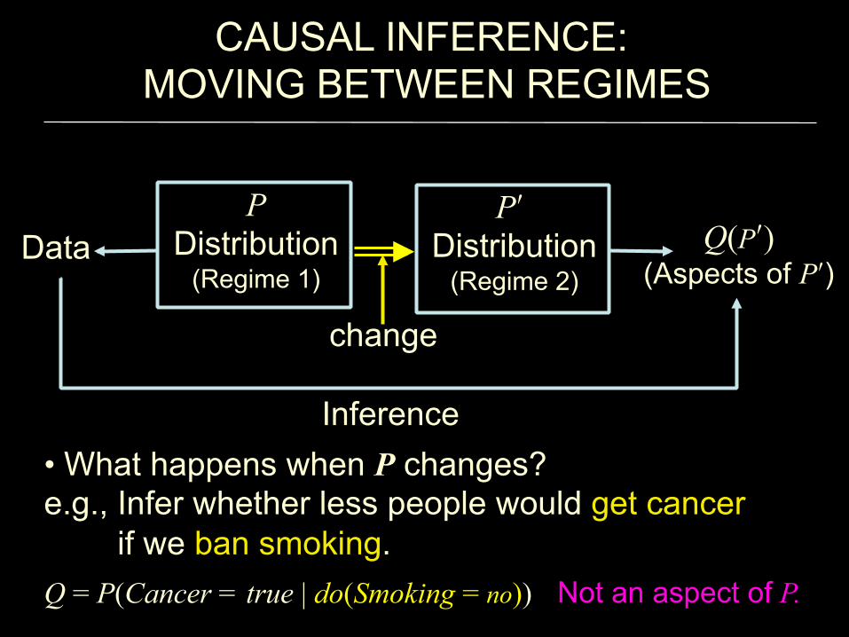
• What happens when P changes? e.g., Infer whether less people would get cancer if we ban smoking.
Q = P(Cancer = true | do(Smoking = no)) !
CAUSAL INFERENCE: MOVING BETWEEN REGIMES!
Data!
Inference!
Q(Pʹ′) (Aspects of Pʹ′)!
Pʹ′ Distribution
(Regime 2) !
P Distribution
(Regime 1) !
change!
Not an aspect of P.!

Observation 1:
The distribution alone tells us nothing about change; it just describes static conditions of a
population (under a specific regime). Observation 2:
We need to be able to represent “change,” or how the population reacts when it
undergoes change in regimes. !

THE BIG PICTURE: THE CHALLENGE OF CAUSAL INFERENCE!
Alternative world!
X! Y!
Z!
W!
• Goal: how much Y changes with X if we vary X between two different constants free from the influence of Z.
• This is the definition of causal effect.!
Z: age, sex X: action W: mediator Y: outcome !
Real world!
X! Y!
Z!
W!change!
P(z, x, w, y) P(y | do(x))

METHOD FOR COMPUTING CAUSAL EFECTS: RANDOMIZED EXPERIMENTS!
Alternative world!
X! Y!
Z!
W!
do(X0)
X0! Y!
Z!
W!
do(X1)
X1! Y!
Z!
W!
P(y | do(X0)) P(y | do(X1)) Randomization:!
Real world!
X! Y!
Z!
W!change!
Z: age, sex X: action W: mediator Y: outcome !

PROBLEM 1. COMPUTING EFFECTS FROM OBSERVATIONAL DATA!
Alternative world!
X! Y!
Z!
W!
P(y | do(x)) P(z, x, w, y)
Questions: * What is the relationship between P(z, x, w, y) and P(y | do(x))? * Is P(y | do(x)) = P(y | x)?
?!
Real world!
X! Y!
Z!
W!
Z: age, sex X: action W: mediator Y: outcome !
change!
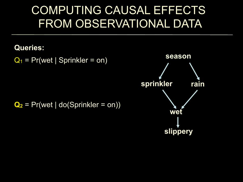
Queries: Q1 = Pr(wet | Sprinkler = on) Q2 = Pr(wet | do(Sprinkler = on))
season!
sprinkler! rain!
wet!
slippery!
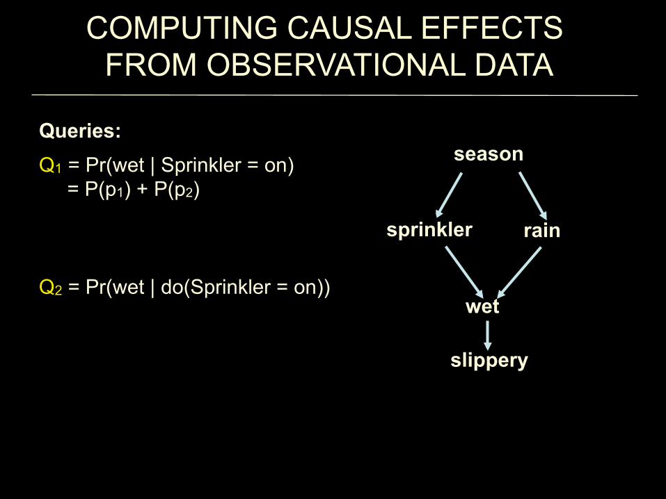
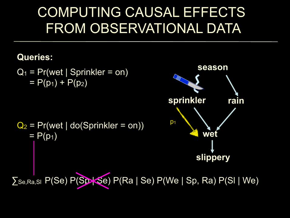
COMPUTING CAUSAL EFFECTS FROM OBSERVATIONAL DATA!

Queries: Q1 = Pr(wet | Sprinkler = on) = P(p1) + P(p2)
Q2 = Pr(wet | do(Sprinkler = on))
season!
sprinkler! rain!
wet!
slippery!
p2!
p1!
COMPUTING CAUSAL EFFECTS FROM OBSERVATIONAL DATA!
season!
sprinkler! rain!
wet!
slippery!
Queries:
Q1 = Pr(wet | Sprinkler = on) = P(p1) + P(p2) Q2 = Pr(wet | do(Sprinkler = on)) !
COMPUTING CAUSAL EFFECTS FROM OBSERVATIONAL DATA!
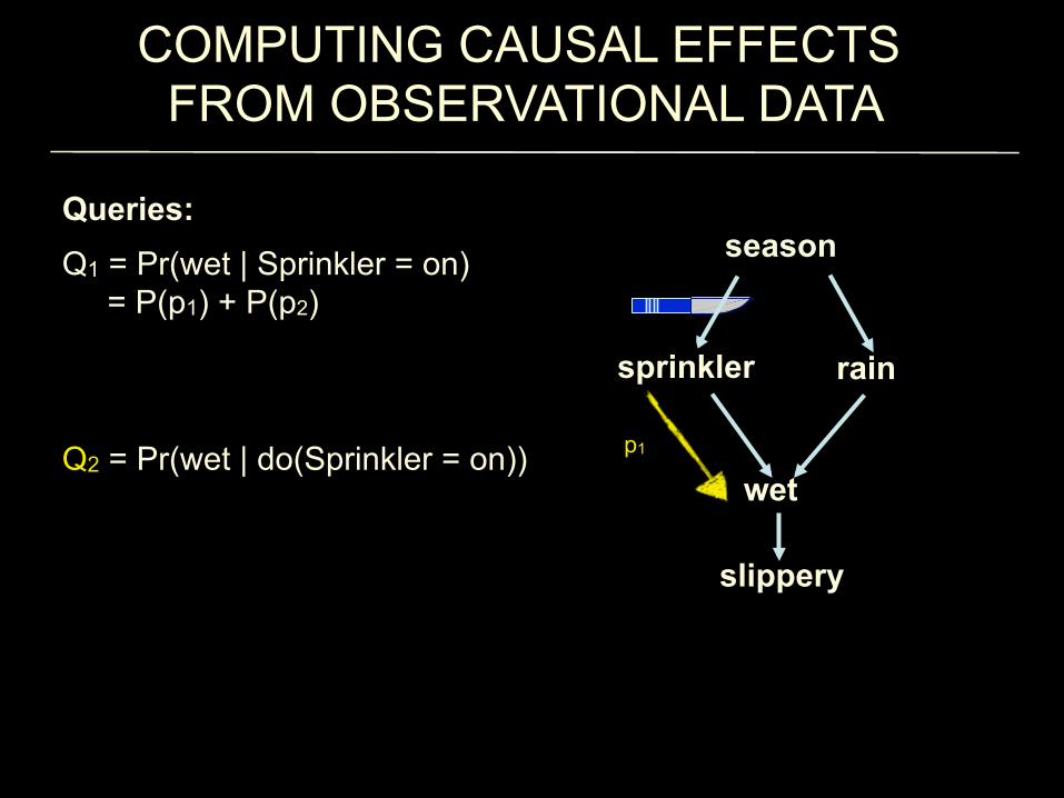
p1!
season!
sprinkler! rain!
wet!
slippery!
Queries: Q1 = Pr(wet | Sprinkler = on) = P(p1) + P(p2)
Q2 = Pr(wet | do(Sprinkler = on)) !
COMPUTING CAUSAL EFFECTS FROM OBSERVATIONAL DATA!

p1!
season!
sprinkler! rain!
wet!
slippery!
Queries: Q1 = Pr(wet | Sprinkler = on) = P(p1) + P(p2)
Q2 = Pr(wet | do(Sprinkler = on)) = P(p1)!
COMPUTING CAUSAL EFFECTS FROM OBSERVATIONAL DATA!
p1!
season!
sprinkler! rain!
wet!
slippery!
Queries: Q1 = Pr(wet | Sprinkler = on) = P(p1) + P(p2)
Q2 = Pr(wet | do(Sprinkler = on)) = P(p1)
∑Se,Ra,Sl P(Se) P(Sp | Se) P(Ra | Se) P(We | Sp, Ra) P(Sl | We)!
COMPUTING CAUSAL EFFECTS FROM OBSERVATIONAL DATA!

OUTLINE!
Concepts:
* Causal inference ⎯ a paradigm shift * The two fundamental laws
Basic tools:
* Graph separation * The truncated product formula * The back-door adjustment formula * The do-calculus
Capabilities:
* Policy evaluation * Transportability * Mediation * Missing Data!
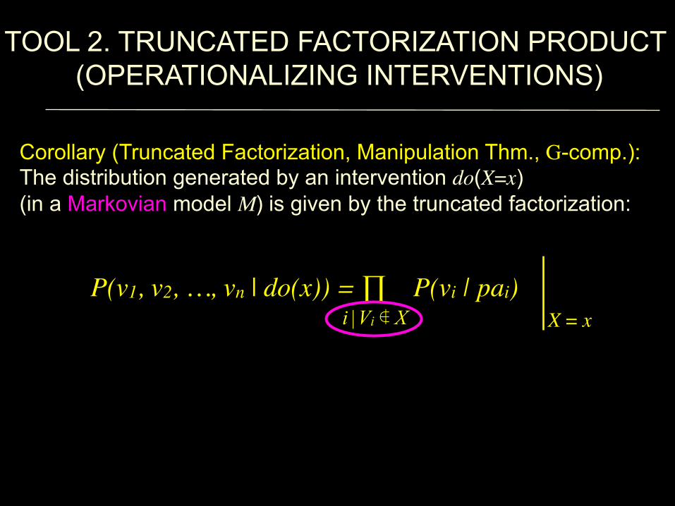
TOOL 2. TRUNCATED FACTORIZATION PRODUCT (OPERATIONALIZING INTERVENTIONS)!
Corollary (Truncated Factorization, Manipulation Thm., G-comp.): The distribution generated by an intervention do(X=x) (in a Markovian model M) is given by the truncated factorization: P(v1, v2, …, vn | do(x)) = ∏ P(vi | pai)
i | Vi ∉ X X = x

NO FREE LUNCH: ASSUMPTIONS ENCODED IN CBNs!
Definition (Causal Bayesian Network):
P(v): observational distribution P(v | do(x)): experimental distribution P*: set of all observational and experimental distributions A DAG G is called a Causal Bayesian Network compatible with P* if and only if the following three conditions hold for every P(v | do(x)) ϵ P*: i. P(v | do(x)) is Markov relative to G; ii. P(vi | do(x)) = 1, for all Vi ϵ X; iii. P(vi | pai, do(x)) = P(vi | pai), for all Vi ∉ X.

OUTLINE!
Concepts:
* Causal inference ⎯ a paradigm shift * The two fundamental laws
Basic tools:
* Graph separation * The truncated product formula * The back-door adjustment formula * The do-calculus
Capabilities:
* Policy evaluation * Transportability * Mediation * Missing Data!

Queries: Q1 = Pr(wet | Sprinkler = on) = P(p1) + P(p2)
Q2 = Pr(wet | do(Sprinkler = on)) = P(p1)
p1!
sprinkler! rain!
wet!
slippery!
∑Se,Ra,Sl P(Se) P(Sp | Se) P(Ra | Se) P(We | Sp, Ra) P(Sl | We)!
IF SEASON IS LATENT, IS THE EFFECT STILL COMPUTABLE?!
p2!
= ∑Ra P(We | Sp, Ra) P(Ra)! Adjustment for direct causes!
= ∑Se P(We | Sp, Se) P(Se)!
season!U!
Adjustment for rain!

TOOL 3. BACK-DOOR CRITERION (THE PROBLEM OF CONFOUNDING)!
Goal: Find the effect of X on Y, P(y|do(x)), given measurements on auxiliary variables Z1,..., Zk!
G !
Z3
Z2
Z5
Z1
X
Z4
Z6 Y

ELIMINATING CONFOUNDING BIAS THE BACK-DOOR CRITERION!
P(y | do(x)) is estimable if there is a set Z of variables that d-separates X from Y in Gx"
Moreover, P(y | do(x)) = ∑ P(y | x,z) P(z) (“adjusting” for Z) !
z!
Gx! G !
Z3
Z2
Z5
Z1
X
Z4
Z6 Y
Z!
Z3
Z2
Z5
Z1
X
Z4
Z6 Y

GOING BEYOND ADJUSTMENT!
Smoking! Tar! Cancer!
Genotype (Unobserved)!
Goal: Find the effect of S on C, P(c | do(s)), given measurements on auxiliary variable T, and when latent variables confound the relationship S-C.!
• What about the effect of S on T, P(t | do(s))? • What about the effect of T on C, P(c | do(t))?

OUTLINE!
Concepts:
* Causal inference ⎯ a paradigm shift * The two fundamental laws
Basic tools:
* Graph separation * The truncated product formula * The back-door adjustment formula * The do-calculus
Capabilities:
* Policy evaluation * Transportability * Mediation * Missing Data!

TOOL 3. CAUSAL CALCULUS (IDENTIFIABILITY REDUCED TO CALCULUS)!
Rule 1: Ignoring observations P(y | do(x), z, w) = P(y | do(x), w),
Rule 2: Action/observation exchange P(y | do(x), do(z), w) = P(y | do(x), z, w),
Rule 3: Ignoring actions P(y | do(x), do(z), w) = P(y | do(x), w), !
The following transformations are valid for every interventional distribution generated by a structural causal model M:

DERIVATION IN CAUSAL CALCULUS!
Smoking! Tar! Cancer!
P (c | do(s)) = Σt P (c | do(s), t) P (t | do(s))!
= Σsʹ′ Σt P (c | do(t), sʹ′) P (sʹ′ | do(t)) P(t |s)!
= Σt P (c | do(s), do(t)) P (t | do(s))!
= Σt P (c | do(s), do(t)) P (t | s)!
= Σt P (c | do(t)) P (t | s)!
= Σsʹ′ Σt P (c | t, sʹ′) P (sʹ′) P(t |s)!
= Σsʹ′ Σt P (c | t, sʹ′) P (sʹ′ | do(t)) P(t |s)!
Probability Axioms!
Probability Axioms!
Rule 2!
Rule 2!
Rule 3!
Rule 3!
Rule 2!
Genotype (Unobserved)!
P (c | do(s))

TECHNICAL NOTE. THE IDENTIFIABILITY PROBLEM!
M1
M2
P1(v) = P2(v) Q1 = Q2
(i.e., ∃ f , f : P(v) → P(y | do(x)))
ID PROBLEM (decision): Given two models M1 and M2 compatible with G that agree on the observable distribution over V, P1(v) = P2(v), decide whether they also agree in the target quantity Q = P(y | do(x)), i.e., whether the effect P(y | do(x)) is identifiable from G and P(v). !

WHAT CAN EXPERIMENTS ON DIET REVEAL ABOUT THE EFFECT OF CHOLESTEROL ON HEART ATTACK?!
Measured:
Observational study: P(x, y, z) Experimental study: P(x, y | do(z))
Needed: Q = P(y | do(x)) = ? !P(x, y | do(z))
P(x | do(z))
Z: Diet X: Cholesterol level Y: Heart Attack !
(i.e., ∃ f , f : P(v), P(v | do(z)) → P(y | do(x)))
=!
G:!
X!
Y!
Z!

WHICH MODEL LICENSES THE z-IDENTIFICATION OF THE CAUSAL EFFECT X→Y ?!
Yes! Yes!No!
No!Yes!No!
(a)! (b)! (c)!
(f)!(e)!(d)!
OUTLINE!
Concepts:
* Causal inference ⎯ a paradigm shift * The two fundamental laws
Basic tools:
* Graph separation * The truncated product formula * The back-door adjustment formula * The do-calculus
Capabilities:
* Policy evaluation * Transportability * Mediation * Missing Data!

SUMMARY OF POLICY EVALUATION RESULTS!
• The estimability of any expression of the form
Q = P(y1, y2, …, yn | do(x1, x2,…,xm), z1,z2,…,zk)
can be determined given any causal graph G containing measured and unmeasured variables.
• If Q is estimable, then its estimand can be derived in
polynomial time (by estimable we mean either from observational or from experimental studies.)!
• The algorithm is complete.
• The causal calculus is complete for this task.

OUTLINE!
Concepts:
* Causal inference ⎯ a paradigm shift * The two fundamental laws
Basic tools:
* Graph separation * The truncated product formula * The back-door adjustment formula * The do-calculus
Capabilities:
* Policy evaluation * Transportability * Mediation * Missing Data!

PROBLEM 2. GENERALIZABILITY AMONG POPULATIONS BREAK (TRANSPORTABILITY)
Question: Is it possible to predict the effect of X on Y in a certain population ∏*, where no experiments can be conducted, using experimental data learned from a different population ∏? Answer: Sometimes yes.

HOW THIS PROBLEM IS SEEN IN OTHER SCIENCES? (e.g., external validity, meta-analysis, ...)
• “Extrapolation across studies requires `some understanding of the reasons for the differences.’” (Cox, 1958)
• “`External validity’ asks the question of generalizability: To what populations, settings, treatment variables, and measurement variables can this effect be generalized?” (Shadish, Cook and Campbell, 2002)
!
• “An experiment is said to have “external validity” if the distribution of outcomes realized by a treatment group is the same as the distribution of outcome that would be realized in an actual program.” (Manski, 2007)

MOVING FROM THE “LAB” TO THE “REAL WORLD” ...
Lab!
Real world!
H1!
H2!
X! Y!
Z!
W!
X! Y!
Z!
W!
Everything is assumed to be the same, trivially transportable!!
Everything is assumed to be different, not transportable...!X! Y!
Z!
W!

R: Π (LA) Π* (NY)!
MOTIVATION
WHAT CAN EXPERIMENTS IN LA TELL US ABOUT NYC?!
Experimental study in LA Measured:
Observational study in NYC Measured:!
X (Intervention)!
Y (Outcome)!
Z (Age)!
Transport Formula (calibration): R =!
Needed: R =!

TRANSPORT FORMULAS DEPEND ON THE CAUSAL STORY!
a) Z represents age
X! Y!
Z!
(b)!
S!
(a)!X! Y!
(c)!Z!
S!
X! Y!
Z! S!
b) Z represents language skill !
c) Z represents a bio-marker !
?!
?!

SEMANTICS FOR TRANSPORTABILITY SELECTION DIAGRAMS!
(G* )!
X! Y!
Z!
W!
X! Y!
Z!
W!
S1! S2!
(G)!
X! Y!W!
Z!
• How to encode disparities and commonalities about domains?!
(D )! fz (uz ) = f *z(uz )
fw(x,uw ) = f *w(x,uw )
fx (z,ux ) ≠ f *w(z,ux )
fy(w, z,uy ) ≠ f *y(w, z,uy )

= P(y | do(x),w)P(w | s)w∑
= P(y | do(x),w)P*(w)w∑
= P(y | do(x), s,w)P(w | do(x), s)w∑
R(= P*(y | do(x)) = P(y | do(x), s)
TRANSPORTABILITY REDUCED TO CALCULUS
Theorem A causal relation R is transportable from ∏ to ∏* if and only if it is reducible, using the rules of do-calculus, to an expression in which S is separated from do( ).
X Y
Z
S
W
60

U
W
RESULT: ALGORITHM TO DETERMINE IF AN EFFECT IS TRANSPORTABLE
X Y Z
V
S T
INPUT: Annotated Causal Graph OUTPUT: 1. Transportable or not? 2. Measurements to be taken in the
experimental study 3. Measurements to be taken in the
target population 4. A transport formula 5. Completeness (Bareinboim, 2012)
S Factors creating differences
P*(y | do(x)) =P(y | do(x), z) P *(z |w)
w∑
z∑ P(w | do(w),t)P *(t)
t∑
S '
61

X! Y!
(f)!Z!
S!
X! Y!
(d)!Z!
S!
W!
WHICH MODEL LICENSES THE TRANSPORT OF THE CAUSAL EFFECT X→Y!
(c)!X! Y!Z!
S!
Y!
(e)!Z!
S!
W! Y!Z!
S!
W!X! Y!Z!
S!
W!
(b)!Y!X!
S!
(a)!Y!X!
S!
Yes! Yes!No!
Yes! No!Yes!

FROM META-ANALYSIS TO META-SYNTHESIS!
The problem How to combine results of several experimental and observational studies, each conducted on a different population and under a different set of experimental conditions, so as to construct an aggregate measure of effect size that is "better" than any one study in isolation. !

META-SYNTHESIS AT WORK!
X! Y!
(f)! Z!
W!
X! Y!
(b)! Z!
W! X! Y!
(c)! Z!
S!
W!X! Y!
(a)! Z!
W!
X! Y!
(g)! Z!
W!
X! Y!
(e)! Z!
W!
S! S!
Target population R = P*(y | do(x))!
X! Y!
(h)! Z!
W! X! Y!
(i)! Z!
S!
W!
S!
X! Y!
(d)! Z!
W!

SUMMARY OF TRANSPORTABILITY RESULTS!
• Nonparametric transportability of experimental results from multiple environments and limited experiments can be determined provided that commonalities and differences are encoded in selection diagrams.
• When transportability is feasible, the transport formula can be derived in polynomial time.
• The algorithm is complete.
• The causal calculus is complete for this task.

OUTLINE!
Concepts:
* Causal inference ⎯ a paradigm shift * The two fundamental laws
Basic tools:
* Graph separation * The truncated product formula * The back-door adjustment formula * The do-calculus
Capabilities:
* Policy evaluation * Transportability * Mediation * Missing Data!

MEDIATION: A GRAPHICAL-COUNTERFACTUAL
SYMBIOSIS 1. Why decompose effects?
2. What is the definition of direct and indirect effects?
3. What are the policy implications of direct and indirect effects?
4. When can direct and indirect effect be estimated consistently from experimental and nonexperimental data?
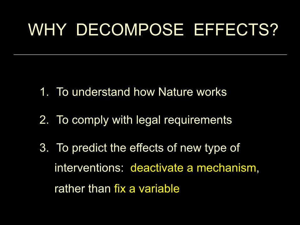
WHY DECOMPOSE EFFECTS?
1. To understand how Nature works
2. To comply with legal requirements
3. To predict the effects of new type of
interventions: deactivate a mechanism,
rather than fix a variable
X Z
Y
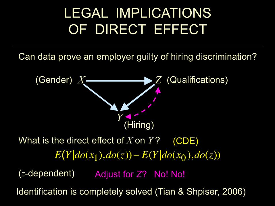
LEGAL IMPLICATIONS OF DIRECT EFFECT
What is the direct effect of X on Y ? (z-dependent)
(Qualifications)
(Hiring)
(Gender)
Can data prove an employer guilty of hiring discrimination?
Adjust for Z?
Identification is completely solved (Tian & Shpiser, 2006)
(CDE)
No! No!
E(Y |do(x1),do(z))− E(Y |do(x0 ),do(z))

z = f (x, u) y = g (x, z, u)
X Z
Y
NATURAL INTERPRETATION OF AVERAGE DIRECT EFFECTS
Natural Direct Effect of X on Y: The expected change in Y, when we change X from x0 to x1 and, for each u, we keep Z constant at whatever value it attained before the change. In linear models, DE = Controlled Direct Effect
Robins and Greenland (1992), Pearl (2001)
DE(x0, x1;Y )
= β(x1 − x0 )E[Yx1Zx0
−Yx0 ]

z = f (x, u) y = g (x, z, u)
X Z
Y
DEFINITION OF INDIRECT EFFECTS
Indirect Effect of X on Y: The expected change in Y when we keep X constant, say at x0, and let Z change to whatever value it would have attained had X changed to x1. In linear models, IE = TE - DE
IE(x0, x1;Y )
No controlled indirect effect
E[Yx0Zx1−Yx0 ]

POLICY IMPLICATIONS OF INDIRECT EFFECTS
f
GENDER QUALIFICATION
HIRING
What is the indirect effect of X on Y?
The effect of Gender on Hiring if sex discrimination is eliminated.
X Z
Y
IGNORE
Deactivating a link – a new type of intervention

THE MEDIATION FORMULAS IN UNCONFOUNDED MODELS
DE = [E(Y | x1, z)− E(Y | x0, z)]P(z | x0 )z∑
IE = [E(Y | x0, z)[P(z | x1)− P(z | x0 )z∑ ]
TE = E(Y | x1)− E(Y | x0 )Fraction of responses explained by mediation (sufficient) Fraction of responses owed to mediation (necessary)
TE ≠ DE + IE
TE − DE =
IE =
X
Z
Y
z = f (x, u1) y = g (x, z, u2) u1 independent of u2

Complete identification conditions for confounded models with multiple mediators (Pearl 2001; Shpitser 2013).
THE MEDIATION FORMULAS IN UNCONFOUNDED MODELS
DE = [E(Y | x1, z)− E(Y | x0, z)]P(z | x0 )z∑
IE = [E(Y | x0, z)[P(z | x1)− P(z | x0 )z∑ ]
TE = E(Y | x1)− E(Y | x0 ) TE ≠ DE + IE
X
Z
Y
z = f (x, u1) y = g (x, z, u2) u1 independent of u2
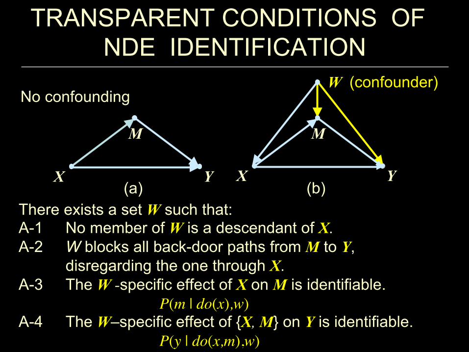
There exists a set W such that: A-1 No member of W is a descendant of X. A-2 W blocks all back-door paths from M to Y,
disregarding the one through X. A-3 The W -specific effect of X on M is identifiable.
P(m | do(x),w) A-4 The W–specific effect of {X, M} on Y is identifiable.
P(y | do(x,m),w)
M
X Y
M
X Y (a) (b)
W (confounder) No confounding
TRANSPARENT CONDITIONS OF NDE IDENTIFICATION

M
Y W2
T W3
M W2
Y T W3
M
Y
W2
T W3
M
Y W2
T W3
(b) M
Y
W2
T W3
(a) M
Y
W2
T W3
(c)
(e) (d) (f)
WHEN CAN WE IDENTIFY MEDIATED EFFECTS?

M
Y W2
T W3
M W2
Y T W3
M
Y
W2
T W3
M
Y W2
T W3
(b) M
Y
W2
T W3
(a) M
Y
W2
T W3
(c)
(e) (d) (f)
WHEN CAN WE IDENTIFY MEDIATED EFFECTS?
W1

SUMMARY OF RESULTS ON MEDIATION
• Ignorability is not required for identifying natural effects
• The nonparametric estimability of natural (and controlled) direct and indirect effects can be determined in polynomial time given any causal graph G with both measured and unmeasured variables.
• If NDE (or NIE) is estimable, then its estimand can be derived in polynomial time.
• The algorithm is complete and was extended to any path-specific effect by Shpitser (2013).
OUTLINE!
Concepts:
* Causal inference ⎯ a paradigm shift * The two fundamental laws
Basic tools:
* Graph separation * The truncated product formula * The back-door adjustment formula * The do-calculus
Capabilities:
* Policy evaluation * Transportability * Mediation * Missing Data!

MISSING DATA: A CAUSAL INFERENCE PERSPECTIVE
(Mohan, Pearl & Tian 2013)
• Pervasive in every experimental science.
• Huge literature, powerful software industry, deeply entrenched culture.
• Current practices are based on statistical characterization (Rubin, 1976) of a problem that is inherently causal.
• Needed: (1) theoretical guidance, (2) performance guarantees, and (3) tests of assumptions. 80

WHAT CAN CAUSAL THEORY DO FOR MISSING DATA?
Q-1. What should the world be like, for a given statistical procedure to produce the expected result?
Q-2. Can we tell from the postulated world whether any method can produce a bias-free result? How?
Q-3. Can we tell from data if the world does not work as postulated?
• To answer these questions, we need models of the world, i.e., process models.
• Statistical characterization of the problem is too crude, e.g., MCAR, MAR, MNAR.
recoverable non-recoverable
testable untestable

Graphical Models for Inference With Missing Data Karthika Mohan, Judea Pearl and Jin Tian
Distribution with missing values
Graph depicting the missingness process
Observed proxy of Z Z*
Treatment
Discomfort
Outcome
Cause of missingness in Z
Z
X
Y
RZ
X Y Z* RZ P(Z*,X,Y,RZ)
0 0 0 0 0.01
0 0 1 0 0.21
0 1 0 0 0.01
0 1 1 0 0.04
1 0 0 0 0.02
1 0 1 0 0.20
1 1 0 0 0.05
1 1 1 0 0.08
0 0 m 1 0.01
0 1 m 1 0.02
1 0 m 1 0.30
1 1 m 1 0.05
(From Mohan et al., NIPS-2013)
82
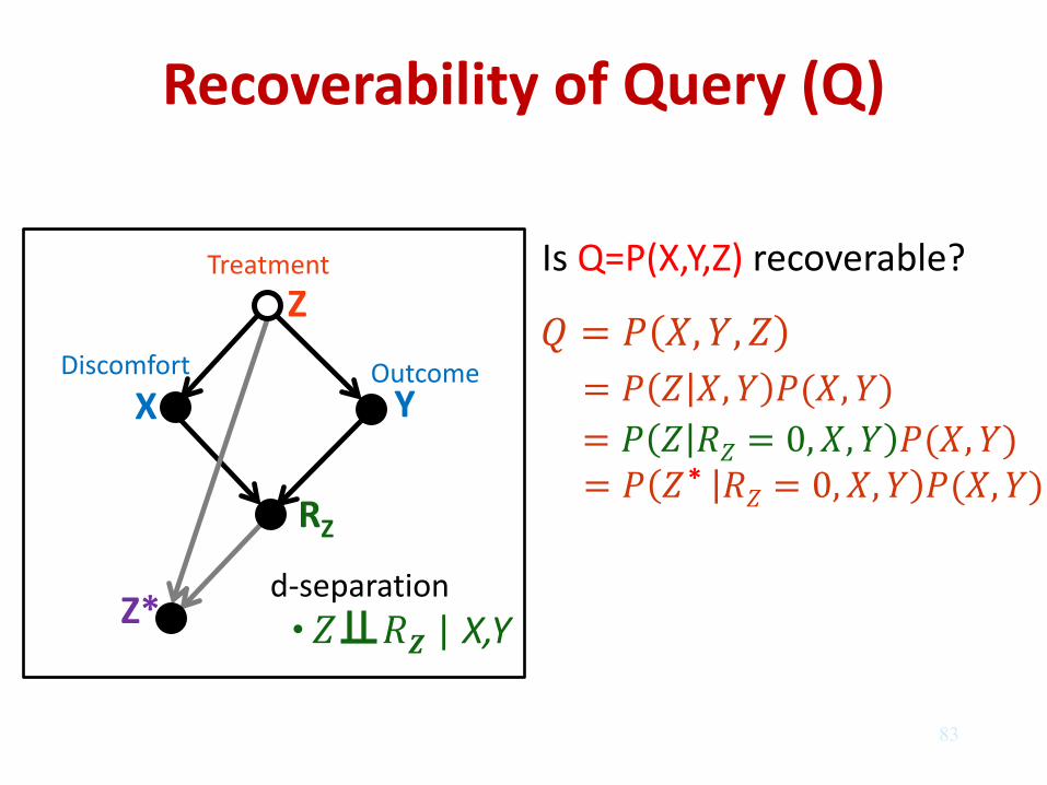
Recoverability of Query (Q) A given query Q is termed recoverable if in the limit of large samples a consistent estimate of Q can be computed given both data and graph, as if no data were missing.
Z*
Treatment
Discomfort
Outcome
Z
X
Y
RZ
= ,, = , (,)
= = 0,, (,) = = 0,, (,)
X,Y | d-separation •
Is Q=P(X,Y,Z) recoverable?
*
83

WHY GRAPHS?
1. Match the organization of human knowledge
1a. Guard veracity of assumptions 1b. Assure transparency of assumptions 1c. Assure transparency of their logical
ramifications
2. Blueprints for simulation 3. Unveil testable implications
x y z w
⇒ x ⊥⊥ wz | y z ⊥⊥ x | y w ⊥⊥ xy | z

Recoverability Given a missingness model G and data D, when is a quantity Q estimable from D without bias?
Non-recoverability Theoretical impediment to any estimation strategy
Testability Given a model G, when does it have testable implications (refutable by some partially-observed data D' )?
What is known about Recoverability and Testability?
RECOVERABILITY AND TESTABILITY
MCAR recoverable almost testable MAR recoverable uncharted MNAR uncharted uncharted

Y X
RX RY
Z Y X
RZ RY
(a)
(g)
RX
(d)
Y X
RX RY P(X)
IS P(X,Y) RECOVERABLE?
Y X
RX RY
Y X
RX RY
Z Y X
RY RX RZ
X Y Z
RX RY RZ
Y X
RX RY Z
Y X
RX (b) (c)
(e) (f)
(h) (i)
RY P(X |Y )
P(X,Y ,Z )
P(X,Y ,Z )

WHAT IF WE DON’T HAVE THE GRAPH?
1. Constructing the graph requires less knowledge than deciding whether a problem lies in MCAR, MAR or MNAR.
2. Understanding what the world should be like for a given procedure to work is a precondition for deciding when model's details are not necessary. (no universal estimator)
3. Knowing whether non-convergence is due to theoretical impediment or local optima, is extremely useful.
4. Graphs unveil when a model is testable.
CONCLUSIONS CONCLUSIONS
1. Think nature, not data, not even experiment.
2. Think hard, but only once – the rest is mechanizable.
3. Speak a language in which the veracity of each
assumption can be judged by users, and which tells you whether any of those assumptions can be refuted by data.

Thank you