AIAA JOURNAL

Vol. 42, No. 5, May 2004

Cavity Flow in Scramjet Engine by Space–TimeConservation and Solution Element Method

Chang-Kee Kim,∗ S.-T. John Yu,† and Zeng-Chan Zhang‡

The Ohio State University, Columbus, Ohio 43210-1154

Numerical simulation of supersonic flows over open cavities in the setting of a dual-mode ramjet/scramjet engineare reported. To calculate the unsteady cavity flows, we employ the space–time conservation element and solutionelement (CESE) method, a novel numerical method based on a unified treatment of space and time for calculationof flux balance. Supersonic cavity flows with and without fuel injection are studied to understand the mechanisms ofmixing enhancement and flame holding by cavities. Without injection, numerical results compared favorably withthe experimental data for dominant frequencies and time-averaged pressure coefficients inside the cavities. Withan upstream injection, the flow oscillations are drastically suppressed. In a downstream injection arrangement,cavity-generated acoustic waves and vortices greatly enhance fuel/air mixing. Numerical results show that theCESE method provides high-fidelity numerical results of unsteady flows in the advanced scramjet engine concept.

I. Introduction

F UEL injection, ignition, and flameholding are challenging is-sues for high-speed combustion. In a viable scramjet engine, the

fuel injection method employed must provide rapid fuel/air mixingwith minimum total-pressure loss in the airstream. A stable flame-holding system under a wide range of operating conditions is crit-ical to sustain the supersonic combustion. Recently, cavity-basedflameholders, an integrated mixing-enhancement and flameholdingapproach, have attracted considerable attention in the scramjet com-munity. Under suitable conditions, flow recirculation, or the trappedvortices, significantly increases the flow residence time of the fluidentering the cavity. A pilot flame could be set up inside the cavity toprovide a pool of hot chemical radicals, which in turn would reducethe ignition delay of the air/fuel mixture in the airstream and, thus,sustain high-speed combustion.

High-speed cavity flows are inherently unsteady, involving bothbroadband small-scale fluctuations typical of turbulent flows, aswell as distinct resonance with harmonic properties in its frequen-cies and amplitudes. In the past, it has been demonstrated that theaspect ratio of the cavity and freestream flow conditions are thecritical parameters dominating the complex flow features, includingboundary-layer separation, compressible free shear layer with shed-ding vortices, linear/nonlinear acoustic waves, and complex shockand expansion waves interacting with vortices and acoustic waves.

In the setting of wheel wells and bomb bays, previous studiesfor high-speed cavity flows showed that cavity flows could be cate-gorized into the following two groups: 1) open cavity flows, whenL/D < 7 ∼ 10, and 2) closed cavity flows, when L/D > 7 ∼ 10,where L denotes the length of the cavity and D the depth. In flowsover cavities of large aspect ratios (L/D > 7 ∼ 10), the separatedfree shear layer emanating from the upstream corner of the cav-

Received 3 August 2002; revision received 18 November 2003; acceptedfor publication 17 December 2003. Copyright c© 2004 by the AmericanInstitute of Aeronautics and Astronautics, Inc. The U.S. Government has aroyalty-free license to exercise all rights under the copyright claimed hereinfor Governmental purposes. All other rights are reserved by the copyrightowner. Copies of this paper may be made for personal or internal use, oncondition that the copier pay the $10.00 per-copy fee to the Copyright Clear-ance Center, Inc., 222 Rosewood Drive, Danvers, MA 01923; include thecode 0001-1452/04 $10.00 in correspondence with the CCC.

∗Research Associate, Mechanical Engineering Department; currentlySenior Scientist, Agency for Defense Development, Tech 3-7, Yuseong, P.O.Box 35-5, Daejon 305-600, Republic of Korea. Member AIAA.

†Associate Professor, Mechanical Engineering Department; yu.274@osu.edu. Member AIAA.

‡Research Associate, Mechanical Engineering Department; currentlySenior Engineer, Livermore Software, 7374 Las Positas Road, Livermore,CA 94550. Member AIAA.

ity reattaches to the bottom wall of the cavity and results in twoseparated recirculation zones near the two corners between the lat-eral walls and the cavity floor. The resultant low-pressure zones atthe lower corners and high pressures on the cavity floor, where theshear layer reattaches, lead to significant drag and pressure loss ofthe airstream. In this case, mass addition/ejection into/from the cav-ity by aerodynamic unsteadiness is low to moderate, and the flow isreferred to as closed.

On the other hand, flows over cavities with smaller aspect ratios,L/D < 7 ∼ 10, result in reattachment of the free shear layer to therear bulkhead of the cavity. The impingement of the free shear layeron the rear lateral wall causes violent unsteady motions and results insignificant periodical mass addition/ejection near the rear bulkheadof the cavity. These flows are referred to as open. The wave patternsof open cavity flows could be further categorized into 1) transversemode for very short cavities, L/D ∼= 1, and 2) longitudinal mode forlonger cavities, for example, 2 ∼ 3 < L/D < 7 ∼ 10. In short cavi-ties, L/D < 2, only one main vortex inside the cavity is sustainedby the driving shear layer spanning the top of the cavity. The upand down motions of the single main recirculation bubble gener-ate acoustic waves, which by and large propagate in the directionperpendicular to the free shear layer, provided the freestream is tran-sonic. The propagating waves are referred to as in a transverse mode.On the other hand, when the cavity is longer, 2 ∼ 3 < L/D < 7 ∼ 10,multiple moving vortices occur inside the cavity leading to complexinteractions among trapped vortices, propagating and reboundingpressure waves, and the flapping free shear layer. In general, the re-bounding pressure waves, while interacting with the free shear layer,drastically amplify the growth rate of the free shear layer, which,in turn, sheds enormous vortices propagating toward and impingingon the aft wall of the cavity. Because of propagating vortices in thestreamwise direction and the rebounding pressure waves, prevalentacoustic waves propagate in the longitudinal direction outside thecavity into the downstream area. If the airstream is transonic or sub-sonic, the acoustics would transversely propagate into the upstreamareas.

In the setting of supersonic combustion inside a scramjet engine,trapped vortices inside cavities could be useful for flameholding.Moreover, cavity resonance, which produces periodic mass addi-tion/expulsion with large flow structures, could be useful for mixingenhancement. Simultaneously, cavity drag must be minimal, for ex-ample, much less than that of a bluff body, and thereby only causeacceptable pressure loss. Gruber et al.1,2 have developed a dual-mode ramjet/scramjet engine concept, which is envisioned to usehydrocarbon fuels for a flight regime of Mach numbers from 3 to6 ∼ 9. In their supersonic combustors,1,2 open cavities with aspectratios about 5 < L/D < 8 have been tested in conjunction with var-ious fuel injection schemes. Numerical simulation of cavity flows

912

KIM, YU, AND ZHANG 913

has been conducted by Baurle et al.3 The results showed that thecavities have great potential to be a viable combined flameholder/mixing enhancement device for a scramjet engine combustor. Sim-ilar ideas have also been independently proposed and tested by Yuet al.4 In particular, Yu et al.4 have tested supersonic flows passingmultiple cavities. Some of recent results have been summarized byBen-Yakar and Hanson.5

In the past, extensive experimental and theoretical studies oncavity flows have been conducted for applications in wheel wellsand bomb bays, and flow characteristics such as the oscillation fre-quency and amplitudes at various locations in the cavity have beenreported.6−11 However, it is difficult to apply this knowledge base di-rectly to cavity flows for the advanced scramjet engines due to muchshorter length/timescales in scramjet engines. Additional complex-ity associated with fuel injection also warrants further studies be-cause cavity flows and the associated acoustics would be drasticallychanged by the fuel injection schemes employed. In particular, in-herent oscillations of cavity flows may be significantly suppressedby an upstream injection.4,9−11

In the present paper, we focus on time-accurate calculation of su-personic cavity flows in the setting of a dual-mode ramjet/scramjetengine combustor.1,2 The objectives of the present study are 1) to val-idate the numerical results by assessment of the calculated frequen-cies and amplitudes of pressure oscillations and comparison withpreviously reported data, 2) to assess the fuel/air mixing enhance-ment based on the application of upstream as well as downstreaminjection to cavity flows, and 3) to demonstrate the capabilities ofthe conservation element and solution element (CESE) method forcapturing complex flow features of the supersonic cavity flows.

The rest of the paper is organized as follows. Section II is a reviewof the model equations to be solved by the CESE method. Section IIIprovides background information on the CESE method. Section IVshows numerical solutions, including comparison between the nu-merical results and previously reported data. Moreover, we willshow the effects by both upstream and downstream injection onpressure oscillations, acoustics, and vortices, leading to effects onfuel/air mixing and flameholding. We then offer concluding remarksand provide cited references.

II. Governing EquationsThe fundamental behavior of cavity flows was known to be

two-dimensional.8 Equation (1) shows the vector form of the two-dimensional flow equations in Cartesian coordinates, including thecontinuity equation, the Navier–Stokes equations, the energy equa-tion, and one species equation:

∂U∂t

+ ∂F∂x

+ ∂G∂y

− ∂Fv

∂x− ∂Gv

∂y= 0 (1a)

where the flow variable vector

U =

ρ

ρu

ρv

ρe

ρY f

(1b)

the inviscid flux vectors are

F =

ρu

ρu2 + p

ρuv

u(ρe + p)

ρuY f

, G =

ρv

ρuv

ρv2 + p

v(ρe + p)

ρvY f

(1c)

and the viscous flux vectors are

Fv =

0

τxx

τxy

uτxx + vτxy − qx

−ρu f Y f

, Gv =

0

τxy

τyy

uτxy + vτyy − qy

−ρv f Y f

(1d)

In the preceding equations, ρ is the density; u and v are velocitycomponents in the x and the y directions, respectively; p is thestatic pressure; and e = ε + 1

2 (u2 + v2) is the specific total energywith ε as the specific internal energy. We assume the fluid is idealand polytropic. Because of the equation of state of an ideal gas,p = (γ − 1)ρε, where γ = Cp/Cv is the specific heat ratio, and itis a constant due to the polytropic gas assumption. In the viscousvectors, τxx , τxy , and τyy are stress components; and qx and qy arethe heat conduction fluxes in the x and y directions, respectively.Y f is the mass fraction of fuel. The diffusion velocity components,u and v are calculated by Fick’s law:

Y f u f = −D∂Y f

∂x(2a)

Y f v f = −D∂Y f

∂y(2b)

where D is the mass diffusivity of fuel in the gas mixture. Themolecular viscosity µ is calculated by the use of Sutherland’s law(see Ref. 12), and the Lewis number Le = 1 is assumed to calcu-late the mass diffusivity D. In numerical calculations, the precedinggoverning equations are nondimensionalized by the freestream con-ditions, that is, velocity components by u∞, density by ρ∞, pressureby ρ∞u2

∞, and the total energy by ρ∞u2∞. The subscript ∞ denotes

the freestream condition. The cavity depth d is used as the lengthscale, and the timescale is d/u∞.

III. CESE MethodThe CESE method is a novel numerical framework for high-

fidelity solution of hyperbolic conservation laws. Originally devel-oped in Refs. 13–18, the tenet of the CESE method is a unifiedtreatment of space and time in calculating flux balance. In contrastto modern upwind schemes, no Riemann solver and/or reconstruc-tion procedure is used as the building block of the CESE method. Asa result, the logic and computational counts of the CESE method aresimpler and more efficient. Based on the CESE method, computerprograms for solving unsteady flows in one, two, and three spatialdimensions for structured and unstructured meshes, and for meshescomposed of mixed elements, have been developed. These solvershave been parallelized based on domain decomposition in conjunc-tion with the use of message passing interface (MPI). Because noRiemann solver is used, we have straightforwardly extended theCESE method for flows with complex physical processes, includ-ing detonation, cavitations, and magnetohydrodynamics (MHD).

Previously, various flow phenomena were calculated by the useof the CESE method. In particular, the CESE solver is capable ofcalculating high-speed compressible flow as well as flows at verylow Mach numbers without applying preconditioning to the gov-erning equations. The CESE method is indeed an all-speed solver.Moreover, the CESE method is capable of simultaneously capturingstrong shock waves and the acoustic waves in the same computa-tional domain, despite that the amplitude of the pressure jump acrossthe shock wave would be several orders of magnitude higher thanthat of the acoustic waves.

The CESE method employed in the present paper is based on theuse of quadrilateral cells on the x–y plane,17 which was extendedfrom the original CESE method. Note that the original CESE methodfor two-dimensional flows was designed based on the use of trian-gular cells. In the present paper, a brief discussion of this particularextension of the CESE method is provided. The discussions herewill be focused on the space–time geometry of the CESE method.We remark that the basic structure of the CESE method can alwaysbe easily grasped by visualization of the space–time geometry ofconservation element (CE), solution element (SE), and how they fa-cilitate the space–time integration. The detailed algebraic equationsof the method, perhaps, only reaffirm the structure of the method.We refer the interested readers to the cited references for all details.

To proceed, let E3 denote a three-dimensional Euclidean space, inwhich x1 = x , x2 = y, and x3 = t . Let ∇ · be the divergence operatorin E3, and hm def [( f − fv)m, (g − gv)m, um] for m = 1, 2, 3, 4, and

914 KIM, YU, AND ZHANG

a)

b)

c)

Fig. 1 Space–time geometry of the CESE method: a) surface elementon boundary S(V) of a region V, b) grid points on the x–y plane, andc) SEs and CEs.

5. Here ( f − fv)m, (g − gv)m , and um are the mth components ofF − Fv , G − Gv , and U , respectively, in Eq. (1). Aided by the pre-ceding definition, for each m = 1, 2, . . . , 5, the flow equations (1)become

∇ · hm = 0 (3a)

Apply Gauss’s divergence theorem to Eq. (3a) and we get∮

S(V )

hm · d s = 0 (3b)

As shown in Fig. 1a, S(V ) is the boundary of the space–time regionV in E3 and ds is a surface element vector pointing outward. Equa-tion (3b) states that the total space–time flux hm , leaving volumeV through S(V ), vanishes. All mathematical operations can be car-ried out as though E3 were an ordinary three-dimensional Euclideanspace. The CESE method is designed to integrate Eq. (3b) accuratelyto provide high-fidelity results of evolving um in the space–timedomain.

The CESE method is a family of numerical schemes, with the ascheme13 as its backbone. In contrast to conventional finite volumemethods, the CESE method has separate definitions of CE and SEin the construction of the discretized equations for integration ofEq. (3b) in the space–time domain. CEs are nonoverlapping space–time subdomains such that 1) the whole computational domain canbe filled by the CEs, 2) flux conservation can be enforced over eachCE and/or over a union of several neighboring CEs, and 3) flowdiscontinuity is allowed inside a CE. On the other hand, SE arenonoverlapping space–time subdomains such that 1) SE do not gen-erally coincide with a CE, 2) the union of all SEs does not have to fillthe whole computational domain, 3) flow variables and fluxes arediscontinuous across interfaces of neighboring SEs, and 4) within aSE, flow variable and flux function are assumed continuous, and theyare approximated by the use of a prescribed smooth function. In thepresent paper, a first-order Taylor series expansion is used. Thus, thediscretized flow variables and fluxes are linearly distributed insideeach SE.

The time-marching strategy in the CESE method is designedbased on a space–time staggered mesh stencil composed of CEs

and SEs. Note that when Eq. (3b) is integrated over the boundary ofa CE, the surface element of S(V ) in Eq. (3b) is always lying insidea SE, where flow variables and fluxes are continuous. We remarkthat the paradigm of the Godunov schemes is that one has to resortto the use of a Riemann solver to reckon the nonlinear flux functionat the cell interfaces. In the CESE method, however, flow informa-tion propagates only in one direction across all cell interfaces, thatis, toward the future. Thus, the space–time flux integration can bestraightforwardly carried out without reconciling the values of fluxfunctions at cell interfaces through the use of a Riemann solver. Inother words, in contrast to the upwind methods, there is no cell in-terface across which two-way flow traffic information propagates.Thus, the CESE method can capture shocks without using a Riemannsolver. In what follows, we discuss specific space–time geometry ofthe CE and SE in the integration of Eq. (3b).

Consider Fig. 1b. The x–y plane is divided into nonoverlappingquadrilaterals. Two neighboring quadrilaterals share a common side.Vertices and centroids of quadrilaterals are marked by dots and cir-cles, respectively. Q is the centroid of the quadrilateral B1 B2 B3 B4.A1,A2, A3, and A4, respectively, are the centroids of the four quadri-laterals neighboring the quadrilateral B1 B2 B3 B4. Q∗, marked by across in Fig. 1b, is the centroid of the polygon A1 B1 A2 B2 A3 B3 A4 B4.Hereafter, point Q∗, which generally does not coincide with pointQ, is referred to as the solution point associated with Q. Note thatpoints A∗

1, A∗2, A∗

3, and A∗4, which are also marked by crosses, are

the solution points associated with the centroids A1, A2, A3, and A4,respectively.

To proceed, we consider Fig. 1c. Here t = n�t at the nth timelevel, where n = 0, 1

2 , 1, 32 , etc. For a given n > 0, Q, Q ′, and Q ′′,

respectively, denote the points on the nth, the (1 − 12 n)th, and the

(1 + 12 n)th time levels with point Q being their common spatial

projection. Other space-time mesh points, such as those shownin Fig. 1c, and also those not depicted, are defined similarly.In particular, Q∗, A∗

1, A∗2, A∗

3, and A∗4 lie on the nth time level,

and they are the space–time solution mesh points associated withpoints Q, A1, A2, A3, and A4. Q ′∗, A′∗

1 , A∗2, A′∗

3 , and A′∗4 lie on the

(1 − 12 n)th time level and are the space–time solution mesh points

associated with points Q ′, A′1, A′

2, A′3, and A′

4.With the preceding preliminaries, we are ready to discuss the

geometry of the CE and SE associated with point Q∗, where thenumerical solution of the flow variables um at nth time level arecalculated based on the known flow solution in all points at an earliertime level, that is, n − 1

2 , denoted by superscript prime. First, the SEof point Q∗, denoted by SE(Q∗), is defined as the union of the fiveplane segments Q ′ Q ′′ B ′′

1 B ′1, Q ′ Q ′′ B ′′

2 B ′2, Q ′ Q ′′ B ′′

3 B ′3, Q ′ Q ′′ B ′′

4 B ′4,

and A1 B1 A2 B2 A3 B3 A4 B4 and their immediate neighborhoods.To integrate Eq. (3b), four basic conservation elements (BCEs)

of point Q∗ are constructed, and they are denoted by BCEl(Q),with l = 1, 2, 3, and 4. These four BCEs are defined to be thespace–time cylinders A1 B1 Q B4 A′

1 B ′1 Q ′ B ′

4, A2 B2 Q B1 A′2 B ′

2 Q ′ B ′1,

A3 B3 Q B2 A′3 B ′

3 Q ′ B ′2, and A4 B4 Q B3 A′

4 B ′4 Q ′ B ′

3, respectively. Inaddition, the compounded CE of point Q, denoted by CE(Q),is defined to be the space–time cylinder A1 B1 A2 B2 A3 B3 A4 B4 A′

1B ′

1 A′2 B ′

2 A′3 B ′

3 A′4 B ′

4, that is, the union of the four precedingBCEs.

To proceed, the set of the space–time mesh points whose spatialprojections are the centroids of quadrilaterals depicted in Fig. 1bis denoted by �, and the set of the space–time mesh points whosespatial projections are the solution points depicted in Fig. 1b isdenoted by �∗. Note that the BCEs and the compounded CEs ofany mesh point ∈� and the SE of any mesh point ∈�∗ are definedin a manner identical to that described earlier for point Q and Q∗.With the clear definitions of the CE and SE as stated, the numericalintegration of the space–time flux balance, that is, Eq. (3b), in thepresent modified CESE method can be summarized as follows:

1) For any Q∗ ∈ �∗ and (x, y, t) ∈ SE(�∗), the flow variables andflux vectors, that is, um(x, y, t), fm(x, y, t), and gm(x, y, t), areapproximated to their numerical counterparts, that is, u∗

m(x, y, t),f ∗m(x, y, t), and g∗

m(x, y, t), by the use of the first-order Taylor seriesexpansion with respect to Q∗ (xQ∗ , yQ∗ , tn). Thus, the space–timeflux vector hm(x, y, t), can be replaced by h∗

m(x, y, t; Q∗), and the

KIM, YU, AND ZHANG 915

numerical analog of Eq. (3b) for each m = 1, 2, . . . , 5, is

∮S[C E(Q)]

h∗m · d s = 0 (4)

Equation (4) states that the discretized total flux of h∗m , leaving

CE(Q) through its boundary, vanishes. We note that Eq. (4) can bewritten in terms of independent discrete solution variables that arethe main flow variables and their spatial derivatives, (umx )Q∗ and(umy)Q∗ in this approximation process.

2) When the integration of Eq. (4) is conducted over theCE = BCE1 + BCE2 + BCE3 + BCE4, the discrete flow variables(um)Q∗ associated with the space–time point Q∗ can be straight-forwardly evaluated. This is achieved by the aid of the geometricalinformation of CE(Q∗) as shown in Fig. 1, and the linear distribu-tion of (um)Q∗ in each SE due to the adopted first-order Taylor seriesexpansion for the flow variables inside the SE as the discretizationprocess.

3) The calculation of the gradient variables, that is, (umx )Q∗ and(umy)Q∗ is based on a finite difference approach in conjunction withthe standard CESE artificial damping functions, that is, the a-ε-αscheme, in which parameter ε is associated with the overall dampingeffect and α is for shock capturing. In contrast to the original CESEmethod, the calculation of (umx )Q∗ and (umy)Q∗ has nothing to dowith the space–time flux conservation.

To calculate unsteady flows, the nonreflecting boundary condi-tion treatment is critically important. Without an effective treatment,the reflected waves would inevitably contaminate the evolving flowsolutions. Numerical treatments to achieve nonreflecting boundaryconditions in the setting of conventional computational fluid dynam-ics (CFD) methods have been actively researched for a long time. Ingeneral, most of treatments were developed based on theorems ofthe partial differential equation, and they could be categorized intothe following three groups: 1) application of the method of charac-teristics to the discretized equations, 2) use of the buffer zone or aperfectly matched layer, and 3) application of asymptotic analyticalsolution at the far field.

When the CESE method is set, we are only concerned with theintegral equation. The preceding ideas of treating a nonreflectiveboundary are not applicable. Instead, the nonreflecting boundarycondition treatments when the CESE method is set are based onflux conservation in the vicinity of the computational boundary.18 Inother words, the present nonreflecting boundary condition treatmentis equivalent to letting the incoming flux from the interior domain tothe boundary CE smoothly exit to the exterior of the domain. In thesetting of the CESE method, the numerical implementation of thisflux-based method is extremely simple because all flow informationmust propagate into the future. Chang et al.18 have provided detaileddiscussions of various implementations of the preceding principle. Ithas been demonstrated that only negligible reflection occurs when ashock passes through the domain boundary. Moreover, along a wallboundary, a unified boundary condition for viscous flows is used.Based on local space–time flux conservation, a no-slip condition willbe automatically enforced when the viscosity is not null. Again, thebasic principle is based on the space–time flux conservation overCEs near the computational boundary.

IV. Results and DiscussionThree sets of numerical results are presented: 1) supersonic cavity

flow in the supersonic combustion facility by Gruber et al.1,2 andby Baurle et al.,3 2) Stalling and Wilcox’s cavity flow test,19 and3) cavity flows with fuel injection. The first test is performed toassess the numerical accuracy of the calculated frequencies. Theresults will be compared with previously reported data and Rossiter’sempirical relation (see Ref. 6). The second test is performed to assessthe numerical accuracy of time-averaged amplitudes of pressurefluctuations along the cavity walls. The results will be comparedwith the experimental data.19 In the third test, cavity flows withdownstream, as well as upstream, injections are simulated. We willshow that a cavity flow with a downstream transverse injection can

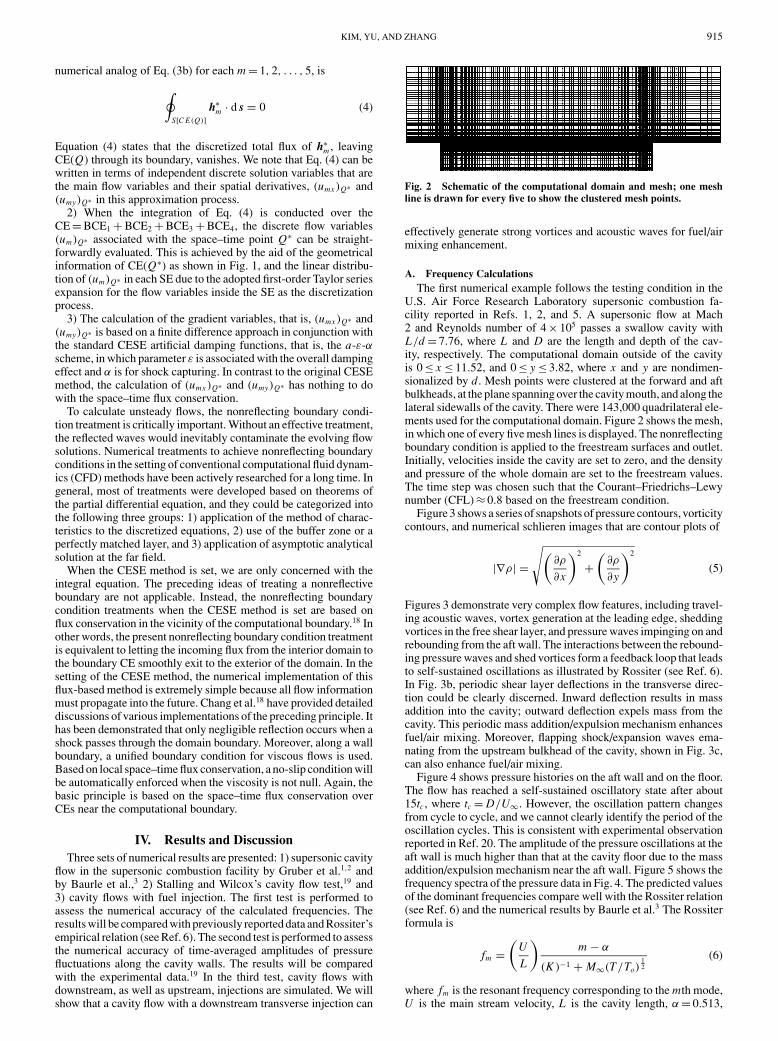
Fig. 2 Schematic of the computational domain and mesh; one meshline is drawn for every five to show the clustered mesh points.

effectively generate strong vortices and acoustic waves for fuel/airmixing enhancement.

A. Frequency CalculationsThe first numerical example follows the testing condition in the

U.S. Air Force Research Laboratory supersonic combustion fa-cility reported in Refs. 1, 2, and 5. A supersonic flow at Mach2 and Reynolds number of 4 × 105 passes a swallow cavity withL/d = 7.76, where L and D are the length and depth of the cav-ity, respectively. The computational domain outside of the cavityis 0 ≤ x ≤ 11.52, and 0 ≤ y ≤ 3.82, where x and y are nondimen-sionalized by d. Mesh points were clustered at the forward and aftbulkheads, at the plane spanning over the cavity mouth, and along thelateral sidewalls of the cavity. There were 143,000 quadrilateral ele-ments used for the computational domain. Figure 2 shows the mesh,in which one of every five mesh lines is displayed. The nonreflectingboundary condition is applied to the freestream surfaces and outlet.Initially, velocities inside the cavity are set to zero, and the densityand pressure of the whole domain are set to the freestream values.The time step was chosen such that the Courant–Friedrichs–Lewynumber (CFL) ≈ 0.8 based on the freestream condition.

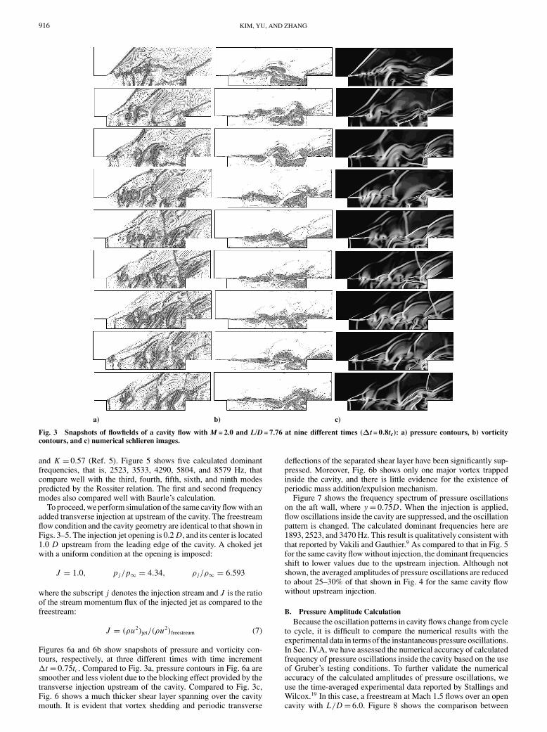
Figure 3 shows a series of snapshots of pressure contours, vorticitycontours, and numerical schlieren images that are contour plots of

|∇ρ| =√(

∂ρ

∂x

)2

+(

∂ρ

∂y

)2

(5)

Figures 3 demonstrate very complex flow features, including travel-ing acoustic waves, vortex generation at the leading edge, sheddingvortices in the free shear layer, and pressure waves impinging on andrebounding from the aft wall. The interactions between the rebound-ing pressure waves and shed vortices form a feedback loop that leadsto self-sustained oscillations as illustrated by Rossiter (see Ref. 6).In Fig. 3b, periodic shear layer deflections in the transverse direc-tion could be clearly discerned. Inward deflection results in massaddition into the cavity; outward deflection expels mass from thecavity. This periodic mass addition/expulsion mechanism enhancesfuel/air mixing. Moreover, flapping shock/expansion waves ema-nating from the upstream bulkhead of the cavity, shown in Fig. 3c,can also enhance fuel/air mixing.

Figure 4 shows pressure histories on the aft wall and on the floor.The flow has reached a self-sustained oscillatory state after about15tc, where tc = D/U∞. However, the oscillation pattern changesfrom cycle to cycle, and we cannot clearly identify the period of theoscillation cycles. This is consistent with experimental observationreported in Ref. 20. The amplitude of the pressure oscillations at theaft wall is much higher than that at the cavity floor due to the massaddition/expulsion mechanism near the aft wall. Figure 5 shows thefrequency spectra of the pressure data in Fig. 4. The predicted valuesof the dominant frequencies compare well with the Rossiter relation(see Ref. 6) and the numerical results by Baurle et al.3 The Rossiterformula is

fm =(

U

L

)m − α

(K )−1 + M∞(T/To)12

(6)

where fm is the resonant frequency corresponding to the mth mode,U is the main stream velocity, L is the cavity length, α = 0.513,

916 KIM, YU, AND ZHANG

a) b) c)

Fig. 3 Snapshots of flowfields of a cavity flow with M = 2.0 and L/D = 7.76 at nine different times (∆t = 0.8tc): a) pressure contours, b) vorticitycontours, and c) numerical schlieren images.

and K = 0.57 (Ref. 5). Figure 5 shows five calculated dominantfrequencies, that is, 2523, 3533, 4290, 5804, and 8579 Hz, thatcompare well with the third, fourth, fifth, sixth, and ninth modespredicted by the Rossiter relation. The first and second frequencymodes also compared well with Baurle’s calculation.

To proceed, we perform simulation of the same cavity flow with anadded transverse injection at upstream of the cavity. The freestreamflow condition and the cavity geometry are identical to that shown inFigs. 3–5. The injection jet opening is 0.2 D, and its center is located1.0 D upstream from the leading edge of the cavity. A choked jetwith a uniform condition at the opening is imposed:

J = 1.0, p j/p∞ = 4.34, ρ j/ρ∞ = 6.593

where the subscript j denotes the injection stream and J is the ratioof the stream momentum flux of the injected jet as compared to thefreestream:

J = (ρu2)jet/(ρu2)freestream (7)

Figures 6a and 6b show snapshots of pressure and vorticity con-tours, respectively, at three different times with time increment�t = 0.75tc. Compared to Fig. 3a, pressure contours in Fig. 6a aresmoother and less violent due to the blocking effect provided by thetransverse injection upstream of the cavity. Compared to Fig. 3c,Fig. 6 shows a much thicker shear layer spanning over the cavitymouth. It is evident that vortex shedding and periodic transverse

deflections of the separated shear layer have been significantly sup-pressed. Moreover, Fig. 6b shows only one major vortex trappedinside the cavity, and there is little evidence for the existence ofperiodic mass addition/expulsion mechanism.

Figure 7 shows the frequency spectrum of pressure oscillationson the aft wall, where y = 0.75D. When the injection is applied,flow oscillations inside the cavity are suppressed, and the oscillationpattern is changed. The calculated dominant frequencies here are1893, 2523, and 3470 Hz. This result is qualitatively consistent withthat reported by Vakili and Gauthier.9 As compared to that in Fig. 5for the same cavity flow without injection, the dominant frequenciesshift to lower values due to the upstream injection. Although notshown, the averaged amplitudes of pressure oscillations are reducedto about 25–30% of that shown in Fig. 4 for the same cavity flowwithout upstream injection.

B. Pressure Amplitude CalculationBecause the oscillation patterns in cavity flows change from cycle

to cycle, it is difficult to compare the numerical results with theexperimental data in terms of the instantaneous pressure oscillations.In Sec. IV.A, we have assessed the numerical accuracy of calculatedfrequency of pressure oscillations inside the cavity based on the useof Gruber’s testing conditions. To further validate the numericalaccuracy of the calculated amplitudes of pressure oscillations, weuse the time-averaged experimental data reported by Stallings andWilcox.19 In this case, a freestream at Mach 1.5 flows over an opencavity with L/D = 6.0. Figure 8 shows the comparison between

KIM, YU, AND ZHANG 917

the present numerical solutions and the experimental data for thetime-averaged pressure coefficient, which is defined as

cp = 2[

p − (1/

γ M2∞)]

(8)

where p is the time-averaged surface pressure. The calculated resultsare in favorable agreement with the experimental data, except nearthe fore wall of the cavity. The discrepancy between the numericalsolution and experimental data is perhaps due to uncertainties of

Fig. 4 Monitored pressure history on the wall.

Fig. 5 Calculated dominant frequencies of the U.S. Air Force ResearchLaboratory testing case.

a) b)

Fig. 6 Cavity flow with an upstream injection; J = 1, M = 2.0, and L/D = 7.76: a) snapshots of pressure contours and b) snapshots of vorticity contours.

Fig. 7 Dominant frequencies for the cavity flow with injection.

Fig. 8 Time-averaged pressure coefficients along the cavity floor in theNASA testing case.

Fig. 9 Schematic diagram of flowfield inside a supersonic-combustionduct.

918 KIM, YU, AND ZHANG

a) b) c)

Fig. 10 Snapshots of flowfields of a cavity flow with downstream injection: a) pressure contours, b) vorticity contours, and c) mole fraction contoursof fuel.

Fig. 11 Pressure oscillations on the cavity wall of an open cavity withdownstream injection.

the incoming boundary layer in the experiments. It can also be dueto the two-dimensional assumption employed in the present paper.The same issue has been discussed by Rizzetta.8

C. Cavity for Fuel/Air Mixing EnhancementResults in Sec. IV.A. show that fuel injection upstream of a cavity

suppresses instability of cavity flows and, thus, is not favorable tobe used for fuel/air mixing enhancement in the setting of a scram-jet engine combustor. To proceed, we simulate a cavity flow witha downstream transverse injection. The cavity geometry and cavityflow conditions are identical to that reported by Gruber et al.21 A su-personic flow at Mach 1.98 (P∞ = 41.8 kPa and ρ∞ = 0.860 kg/m3)passes a cavity with L/D = 7.76 with D = 6.35 mm. In the presentcalculation, hydrogen is the injected fuel. The size and position of theinjection jet opening are shown in Fig. 9. A choked jet with a uniformcondition at the opening is imposed with the following flow condi-tions: J = 1.0, u j = 317 m/s, Pj = 16.4 kPa, ρ j = 2.283 kg/m3.

Figure 10 shows snapshots of pressure, vorticity, and fuelmass fraction contours at five different times with time increment�t = 15 µs. These contour plots show violent interactions between

the fuel jet and the cavity flow, leading to complex pressure wavesand large vortex structures around the aft wall of the cavity and thefuel injection slot. Compared to the feedback mechanism in cavityflows without any injection, the self-sustained flow oscillations hereare much more violent. As a result, the mass addition/expulsion pro-cess near the aft bulkhead of the cavity has been greatly enhancedby the fuel injection downstream of the cavity. Moreover, these en-hanced oscillations near the aft corner cause part of fuel, which wasinjected downstream of the cavity, to move upstream, enter into thecavity and become trapped in recirculation bubbles. Thus, the flowresidence time of the fuel in the combustion chamber significantlyincreases and flameholding characteristics could be improved.

Figure 11 shows the time histories of calculated pressures at twolocations inside the cavity, that is, the center of the cavity floorand near the corner on the aft wall, indicated by filled trianglesin Fig. 11. The flow reaches a self-sustained oscillatory state afterabout 200 µs (∼=16tc). Contrary to the case of the cavity flow withan upstream injection (refer to Fig. 6), downstream injection hereenhances the overall pressure oscillations of the flowfield with muchhigher pressure oscillation amplitudes. Moreover, the amplitudes ofthe pressure oscillations on the floor and on the aft bulkhead arecomparable, whereas, in the case without fuel injection, the pressurefluctuation amplitudes are much larger on the aft bulkhead than thaton the cavity floor.

V. ConclusionsIn the present paper, we applied the CESE method to simulate su-

personic cavity flows in the setting of a dual-mode ramjet/scramjetengine. Two-dimensional Navier–Stokes solvers are solved for threesets of testing conditions. As part of the code validation effort, thecalculated results showed that the CESE method could vividly cap-ture the well-known feedback mechanism and the self-sustained os-cillations in the supersonic cavity flows. We observed cycle-to-cyclechanges in oscillation patterns. The calculated frequencies of pres-sure oscillations at locations inside the cavity compared well withRossiter’s relation (see Ref. 6) and the Baurle et al.3 data. Numericalaccuracy is further validated by favorable comparison between thecalculated amplitudes of pressure oscillations along cavity floor andthe experimental data by Stallings and Wilcox.19

With regard to mixing and flameholding enhancement for su-personic combustion, our results show that an upstream injectiondrastically suppresses flow oscillations. The dominant frequencies

KIM, YU, AND ZHANG 919

of pressure oscillations shift to lower values with much lower ampli-tudes. Moreover, upstream injection induces thicker and more stablefree shear layer spanning over the cavity mouth, leading to vor-tex motions reduced drastically. In general, upstream injection sup-presses the desired mixing and flameholding features for supersoniccombustion. On the other hand, cavity flows with a downstream in-jection show promising potential for mixing and flameholding en-hancement. Because of interactions between flow oscillations nearthe aft bulkhead of the cavity and the injection jet, the amplitudesof the pressure oscillations are greatly amplified as compared to thecase without injection. Large vortices occur, leading to fuel propa-gation upstream in to the cavity, where the recirculation bubbles arehighly unstable. They interact with the pulsating vortex structuredownstream of the cavity. The preceding results warrant further in-vestigation of the fuel injection downstream of an open cavity forpossible fuel/air mixing and flameholding enhancement. In general,numerical results obtained by the CESE method can effectively cap-ture the unsteady and complex mixing processes of cavity flows inthe setting of an advanced scramjet engine.

AcknowledgmentsThis work was funded by the U.S. Air Force Office of Scientific

Research under Grant F49620-01-1-0051. The project is monitoredby J. Schmisseur. The second author is in debt to Douglas Davisand Tom Jackson of the U.S. Air Force Research Laboratory atWright–Patterson Air Force Base for fruitful discussions.

References1Gruber, M. R., Baurle, R. A., Mathur, T., and Hsu, K.-Y., “Fundamental

Studies of Cavity-Based Flame Holder Concepts for Supersonic Combus-tors,” Journal of Propulsion and Power, Vol. 17, No. 1, 2001, pp. 146–153.

2Gruber, M. R., Jackson, K., Mathur, T., and Billig, F., “Experimentswith a Cavity-Based Fuel Injector for Scramjet Applications,” InternationalSociety of Air-Breathing Engines, ISABE Paper IS-7154, Sept. 1999.

3Baurle, R. A., Tam, C.-J., and Dasgupta, S., “Analysis of Unsteady CavityFlows for Scramjet Applications,” AIAA Paper 2000-3617, July 2000.

4Yu, K. H., Wilson, K. J., and Schadow, K. C., “Effect of Flame-HoldingCavities on Supersonic-Combustion Performance,” Journal of Propulsionand Power, Vol. 17, No. 6, 2001, pp. 1287–1295.

5Ben-Yakar, A., and Hanson, R. K., “Cavity Flame-Holders for Ignitionand Flame Stabilization in Scramjets: An Overview,” Journal of Propulsionand Power, Vol. 17, No. 4, 2001, pp. 869–877.

6Tam, C. K. W., and Block, P. J. W., “On the Tones and Pressure Os-cillations Induced by Flow over Rectangular Cavities,” Journal of FluidMechanics, Vol. 89, Pt. 2, 1978, pp. 373–399.

7Rockwell, D., and Naudascher, E., “Review–Self-Sustaining Oscilla-tions of Flow past Cavities,” Journal of Fluids Engineering, Vol. 100, June1978, pp. 152–165.

8Rizzetta, D. P., “Numerical Simulation of Supersonic Flow over a Three-Dimensional Cavity,” AIAA Journal, Vol. 26, No. 7, 1988, pp. 799–807.

9Vakili, A. D., and Gauthier, C., “Control of Cavity Flow by UpstreamMass-Injection,” Journal of Aircraft, Vol. 31, No. 1, 1994, pp. 169–174.

10Sarno, R. L., and Franke, M. E., “Suppression of Flow-Induced PressureOscillations in Cavities,” Journal of Aircraft, Vol. 31, No. 1, 1994, pp. 90–96.

11Lamp, A. M., and Chokani, N., “Computation of Cavity Flows withSuppression Using Jet Blowing,” Journal of Aircraft, Vol. 34, No. 4, 1997,pp. 545–551.

12Anderson, D. A., Tannehill, J. C., and Pletcher, R. H., ComputationalFluid Mechanics and Heat Transfer, McGraw–Hill, New York, 1984, p. 189.

13Chang, S.-C., “The Method of Space–Time Conservation Elementand Solution Element—A New Approach for Solving the Navier–Stokesand Euler Equations,” Journal of Computational Physics, Vol. 119, 1995,pp. 295–324.

14Chang, S.-C., Yu, S.-T., Himansu, A., and Wang, X.-Y., “The Methodof Space–Time Conservation Element and Solution Element—A NewParadigm for Numerical Solution and Conservation Laws,” ComputationalFluid Dynamics Review 1998, edited by M. Hafez and K. Oshima, WorldScientific, London, 1999, pp. 206–240.

15Chang, S.-C., Wang, X.-Y., and Chow, C.-Y., “The Space–Time Con-servation Element and Solution Element Method: A New High-Resolutionand Genuinely Multidimensional Paradigm for Solving Conservation Laws,”Journal of Computational Physics, Vol. 156, 1999, pp. 89–136.

16Chang, S.-C., Wang, X.-Y., and To, W.-M., “Application of theSpace–Time Conservation Element and Solution Element Method to One-Dimensional Convection–Diffusion Problem,” Journal of ComputationalPhysics, Vol. 165, 2000, pp. 189–215.

17Zhang, Z. C., Yu, S.-T. J., and Chang, S. C., “A Space–Time Conserva-tion Element and Solution Element Method for Solving the Two- and Three-Dimensional Euler Equations by Quadrilateral and Hexahedral Meshes,”Journal of Computational Physics, Vol. 175, No. 1, 2002, pp. 168–199.

18Chang, S.-C., Himansu, A., Loh, C. Y., Wang, X.-Y., Yu, S.-T., andJorgenson, P. C. E., “Robust and Simple Non-Reflecting Boundary Con-ditions for the Space-Time Conservation Element and Solution ElementMethod,” AIAA Paper 97-2077, June–July 1997.

19Stallings, R. L., Jr., and Wilcox, F. J., “Experimental Cavity PressureDistributions at Supersonic Speeds,” NASA TP-2683, June 1987.

20Lin, J.-C., and Rockwell, D., “ Organized Oscillations of Initially Turbu-lent Flow past a Cavity,” AIAA Journal, Vol. 39, No. 6, 2001, pp. 1139–1151.

21Gruber, M. R., Nejad, A. S., Chen, T. H., and Dutton, J. C., “Compress-ibility Effects in Supersonic Transverse Injection Flow Fields,” Physics ofFluids, Vol. 9, No. 5, 1997, pp. 1448–1461.

M. SichelAssociate Editor