cawcr research letters 3v4 · 2010-01-28 · cawcr research letters is an internal serial online...
TRANSCRIPT

The Centre for Australian Weather and Climate Research A partnership between CSIRO and the Bureau of Meteorology
CAWCR Research Letters Issue 3, December 2009 P. A. Sandery, T. Leeuwenburg, G. Wang, A. J. Hollis (editors)

ISSN: 1836-5949 Series: Research Letters (The Centre for Australian Weather and Climate Research); Issue 3.
Copyright and Disclaimer
© 2008 CSIRO and the Bureau of Meteorology. To the extent permitted by law, all rights are reserved and no part of this publication covered by copyright may be reproduced or copied in any form or by any means except with the written permission of CSIRO and the Bureau of Meteorology.
CSIRO and the Bureau of Meteorology advise that the information contained in this publication comprises general statements based on scientific research. The reader is advised and needs to be aware that such information may be incomplete or unable to be used in any specific situation. No reliance or actions must therefore be made on that information without seeking prior expert professional, scientific and technical advice. To the extent permitted by law, CSIRO and the Bureau of Meteorology (including each of its employees and consultants) excludes all liability to any person for any consequences, including but not limited to all losses, damages, costs, expenses and any other compensation, arising directly or indirectly from using this publication (in part or in whole) and any information or material contained in it.

http://www.cawcr.gov.au/publications/researchletters.php
Contents A low wind speed parameterisation for stably stratified boundary layers in ACCESS
V. J. I. Barras, A. K. Luhar and P. J. Hurley
4
Comparative verification of 3-hourly guidance from Operational Consensus Forecasts and Model Output Forecasts
W. Lu and F. Woodcock 9
QNH Derivation and Forecasting in the GFE
A. Treloar 14
Impact of SST bias correction on prediction of ENSO and Australian winter rainfall
E.-P. Lim, H. H. Hendon, O. Alves, Y. Yin, M. Zhao, G. Wang, D. Hudson and G. Liu
22
Short-Term Variability of Ozone and UV: A case study
L. L. Lemus-Deschamps, T. Hume and N. Moodie
30
Surface energy balance in the ACCESS models: comparisons with observation based flux products
H. A. Rashid, M. Dix, and A. C. Hirst
35
An analysis of future changes in extreme rainfall over Australian regions based on GCM simulations and Extreme Value Analysis
T. Rafter and D. Abbs
44
Soil Moisture Observation from AMSR-E and its potential use within ACCESS Data Assimilation
J. Lee, P. Steinle and C. Draper
50
Editors: P. A. Sandery, T. Leeuwenburg, G. Wang, A. J. Hollis Enquiries: Dr Paul Sandery [email protected] CAWCR Research Letters The Centre for Australian Weather and Climate Research Bureau of Meteorology GPO Box 1298K Melbourne VICTORIA 3001
CAWCR Research Letters is an internal serial online publication aimed at communication of research carried out by CAWCR staff and their colleagues. It follows on from its predecessor BMRC Research Letters. Articles in CAWCR Research Letters are peer reviewed and typically 4-8 pages in length. For more information visit the CAWCR website.

Parameterisation of SBL wind speeds in ACCESS Page 4 of 55
http://www.cawcr.gov.au/publications/researchletters.php
A low wind speed parameterisation for stably stratified boundary layers in ACCESS
Vaughan J. I. BarrasA, Ashok K. LuharB, Peter J. HurleyC ABCCentre for Australian Weather and Climate Research
ABureau of Meteorology, Melbourne, VIC BCCSIRO Marine and Atmospheric Research, Aspendale, VIC
[email protected], [email protected], [email protected]
Introduction An accurate representation of near-surface winds in global forecast models is important in the calculation of surface energy exchange, air pollution dispersion as well as in aviation and wind engineering applications. In a summary paper, Holtslag (2006) points out that a number of model errors can arise from shortcomings in the representation of the stably stratified planetary boundary layer (SBL). A recent intercomparison of Single Column Models (SCMs), which formed part of the second GEWEX Atmospheric Boundary Layer Study (GABLS2, http://www.met.wau.nl/projects/Gabls/index.htm), found a large spread of results for all model forecast parameters (Svensson and Holtslag, 2007). The greatest difference between the model simulations and observations was in the representation of the diurnal cycle of 10-metre wind speed. The amplitude of this diurnal variation was found to be significantly underpredicted with wind speeds generally too high under nighttime stable conditions. In this paper, model sensitivities to changes in the flux-profile relationships of momentum under stably stratified conditions are investigated using a SCM version of the UK Met Office Unified Model (UM, version 6.3) that forms the atmospheric component of the Australian Community Climate and Earth System Simulator (ACCESS).
Present formulation and testing Flux-profile relationships in the surface layer are commonly described by Monin-Obukhov Similarity Theory (MOST) that expresses the normalised mean gradients as a function of the stability parameter ζ (= z/L, where z is the height
above the surface and L is the Obukhov length scale). The integral of the gradient function for wind speed (ψm) may be used to define departures from the neutral dimensionless wind speed at any level:
( )ζψκ
mzz
uu
−⎟⎟⎠
⎞⎜⎜⎝
⎛≈
0*
ln (1)
where κ is the von Kármán constant (κ = 0.4), u is the mean wind speed (ms-1), *u is the friction velocity (ms-1) and oz is the surface aerodynamic roughness length (m). The boundary layer scheme in the UM currently uses MOST to formulate the stability functions for momentum, heat and moisture (heat and moisture are treated identically). Here our focus is upon the parameterisation of 10-m wind speed, therefore we will only discuss the stability functions for momentum. The current versions of the UM use the integral stability functions of Beljaars and Holtslag (1991) (hereafter BH91):
( ) ( ) ⎟⎟⎠
⎞⎜⎜⎝
⎛+−⎟
⎠⎞
⎜⎝⎛ −+−=
dbcd
dcbam ζζζζψ exp (2)
where a = 1, b = 0.667, c = 5 and d = 0.35. As an indication of the performance of the BH91 stability functions, the SCM was run using forcings from the GABLS2 intercomparison project. GABLS2 utilised observations from the Cooperative Atmosphere-Surface Exchange Study (CASES-99; Poulos et al. 2002) collected in Kansas, USA during October, 1999. The

Parameterisation of SBL wind speeds in ACCESS Page 5 of 55
http://www.cawcr.gov.au/publications/researchletters.php
GABLS2 simulation period was set between 20:00 local time, October 22 until 07:00, October 24 during which two clear-sky diurnal cycles were observed. The second night featured strong to very strong stability near the surface, therefore was of particular interest for this investigation. As described by Svensson and Holtslag (2007), the models significantly overestimated the nocturnal 10m wind speed of October 23-24 (Figure 1). During these periods, the observed ζ values ranged between 0.01-18.9. The degree of error in the ACCESS SCM simulation is difficult to establish due to the gap in the observational coverage of wind speed between 02:00 and 10:00 (during which model ζ values ranged between 0.3-15.8). Observations from nearby locations (grey) show that typical wind speeds during this period were between 1.0-3.5ms-1, indicating the model overestimate to be between ~25-40%.
Figure 1. ACCESS SCM GABLS2 simulation of 10m wind speed (dashed line) with GABLS2 tower observations (dots). Grey markers are reference observations from locations near the main CASES-99 site.
Luhar et al. (2009) stability function for momentum A detailed analysis of low wind speeds under stable conditions was performed by Luhar et al. (2009) (hereon LH09) using field datasets from the CASES-99 intensive observational period (IOP) and Cardington tower operated by the UK Met Office. The analysis found a continuation in the existence of turbulence at ‘super-critical’ values of the gradient Richardson number (Rig > 0.2). It was also noted that the turbulence was weaker and anisotropic in nature, in agreement
with the conclusions of Galperin et al. (2007) and Zilitinkevich et al. (2007). In order to represent the observed transition between turbulent regimes with increasing stability, an alternate approach to the scaling of momentum in the surface layer was devised by LH09. Rather than formulate a new gradient function, a parameterisation was devised which aims to relate the non-dimensional wind speed (κū/u*) directly to ζ. The following form of the non-dimensional wind-speed was chosen and the coefficients α, β and γ were set to fit observations from the Cardington and CASES-99 datasets.
( )[ ]ββ γζζακ −+= 1
*
1u
u (3)
where, α = 4, β = 0.5 and γ = 0.3.
Figure 2. Modified GABLS2 SCM simulation of 10-m wind speed using BH91 (dashed line) and LH09 (solid line) momentum scaling functions for the surface layer.
In an attempt to replicate the observed sharp transition between turbulent regimes, Equation 3 was applied as a step function at the threshold stability ζ > 0.4. To ensure the activation of the new parameterisation under strong stability, the GABLS2 forcings were modified by decreasing the geostrophic wind speed. This had the effect of increasing the nocturnal stability and accentuated the daybreak and dusk transitions (Figure 2).
At the times where the stability exceeded the threshold of ζ = 0.4, the switch to the LH09

Parameterisation of SBL wind speeds in ACCESS Page 6 of 55
http://www.cawcr.gov.au/publications/researchletters.php
stability function resulted in a substantial reduction of 10m wind speed, decreasing wind speeds by between 40-45%. During daytime unstable conditions wind speeds remained unchanged. One feature arising from the sharp transition between the BH91 and LH09 functions was instability in the predictions near the threshold ζ value, most explcitly seen near the end of the simulation. Although a small error, it illustrates a particular sensitivity in the model to the sharpness of the transition. To overcome this, a new approach to the transition between functions was devised.
Application of smoothing function Rather than attempt to formulate a new function to address the model sensitivity, an intermediate smoothing function was applied across a pre-determined transition range as a ‘weighting’ between the BH91 and LH09 functions.
The parameterised non-dimensional wind speed, with smooth transition, is given by the following modification to equation (1):
( ) ( ){ } ( ) ( ){ }⎥⎥⎦
⎤
⎢⎢⎣
⎡−−−−⎟⎟
⎠
⎞⎜⎜⎝
⎛= oLLoBHBH
ozz
uu
ζνζνζψζψκ
ln*
( ) ( ) ( ){ }oLLf ζνζνζ −+⋅ (4)
where ψBH denotes BH91 and νL denotes LH09. Equation (4) introduces the smoothing function
( )ζf based upon the cumulative normal distribution (CND):
( ) ( ) ζσ
μζ
πσζ
ζ
ζ
′⎟⎟⎠
⎞⎜⎜⎝
⎛ −′= ∫
=
dfo 1.0
2
2
2 2exp
2
1 (5)
A numerical solution of the function (5) is found to determine the area fraction under the curve between the lower stability bound (ζ = 0.1) and the atmospheric stability (ζ). As a result, the value of ( )ζf (between 0 and 1) acts as a weighting parameter.
μ = 0.4 ; σ = 1.0
0.1
1
10
100
0.01 0.1 1 10 100
ζ
κU
/u*
BH91LH09Blend
(a)
(b)
Figure 3. Test settings for blended BH91-LH09 momentum stability functions. (a) Smoothed function (red) overlaid upon BH91 (blue) and LH09 (green) (b) Modified GABLS2 SCM simulations of 10-m wind speed using BH91 (dashed line) and smoothed transition to LH09 (solid line).
One of the benefits of using the CND in this context is that it may have its shape adjusted by specification of the distribution mean (μ) and standard deviation (σ). This allows for a certain amount of ‘tuning’ of the stability functions which is helpful in testing the sensitivity of the transition without need to devise new stability functions. Changes in the value of μ may be regarded as a ‘coarse’ tuning by altering the threshold stability for the transition between the functions, whereas a change in the value of σ is a ‘fine’ tuning that results in an adjustment of the ‘sharpness’ of the transition. It should be noted that σ values require a change of the order of a factor of 10 before making a significant difference to the shape function. By experiment it was found that the shape defined by the parameters: μ = 0.4 and σ = 1.0, were effective in removing the instability about the transition threshold (Figure 3). Lesser values of the σ

Parameterisation of SBL wind speeds in ACCESS Page 7 of 55
http://www.cawcr.gov.au/publications/researchletters.php
parameter were too sharp to remove the numerical instability seen in the previous section.
Testing with GABLS 2 SCM forcing Having found an approach that successfully applies the transition between the BH91 and LH09 stability functions, it was necessary to validate the SCM 10m wind speeds against observations. To do this, the forcings for the original GABLS 2 intercomparison were again applied. The settings of the smoothing function were varied to fit observations of non-dimensional wind speed from Cardington, CASES-99 and the Cabauw tower (van Ulden and Wieringa, 1996) in the Netherlands. The different settings were termed BLEND_1, BLEND_2 and BLEND_3 and are detailed in Table 1. The major difference between the BLEND settings is the change in the μ parameter. The small differences in σ have a negligible effect. Variation of the BLEND settings for the GABLS 2 simulations resulted in direct changes to the magnitude of 10m wind speed under stable conditions. The BLEND_1 settings tended to underpredict the nocturnal wind speeds during the GABLS 2 simulation, whereas the BLEND_2 and BLEND_3 settings fell well within the scatter of the observations (Figure 4a). In all cases, however, there was a significant decrease in 10-m wind speeds at night and, therefore, an increase in the diurnal amplitude.
Table 1: Settings for smoothing function f (ζ )
μ σ BLEND_1 0.4 1.00 BLEND_2 1.5 0.80 BLEND_3 2.5 0.96
A useful feature of the new parameterisation is its limited impact upon other model variables. With the application of the different BLEND settings the model representation of friction velocity ( *u ) remained largely unchanged (Figure 4b). The model appeared to capture well the magnitude of
*u during daylight hours but struggled under stable conditions overnight, however there is a high degree of uncertainty in the observations at such low values.
(a)
(b)
Figure 4. GABLS2 SCM simulations of (a) 10m wind speed (ms-1) and (b) friction velocity (ms-1). Dashed line is the BH91 simulation and shaded lines are the BLEND simulations using the smoothing function settings listed in Table 1.
Importantly, the new parameterisation has virtually no effect upon the surface fluxes of heat and moisture. It should be noted that by adjusting the momentum scaling alone, this may induce an imbalance between the stability functions of heat (moisture) and momentum. However, as pointed out by both Beljaars and Holtslag (1991) and Luhar et al. (2009), in the intermittent turbulent regime (Rig > 0.2) the exchange of heat becomes less efficient than that of momentum, therefore any imbalances that may arise under strongly stable conditions from the new parameterisation could reflect those observed in nature.
Conclusions The parameterisation of 10-m wind speeds under stable boundary layer conditions has been

Parameterisation of SBL wind speeds in ACCESS Page 8 of 55
http://www.cawcr.gov.au/publications/researchletters.php
investigated by modifying the integral stability function for momentum in an SCM version of the UM. From a series of experiments it was found that the modelled wind speed was particularly sensitive to the sharpness of the transition between the exisitng stability function of Beljaars and Holtslag (1991) and that of Luhar et al. (2009). Numerical instabilities arising from this sensitivity were overcome by implementing an adjustable smoothing function based upon the cumulative normal distribution that applies a weighting parameter to each of the two functions. Various settings for the smoothing function were tested in order to fit observations used in the GABLS2 SCM intercomparison. The implementation of the new parameterisation was also found to have negligible effect upon other model variables such as temperature and surface fluxes.
Acknowledgements CASES-99 data provided by NCAR/EOL under sponsorship of the National Science Foundation: http://data.eol.ucar.edu/. Cardington Data provided by the UK Met Office. Cabauw data provided by The Royal Netherlands Meteorological Institute (KNMI).
References Beljaars, A.C.M., A.A.M. Holtslag, 1991: Flux parameterization over land surfaces for atmospheric models, Journal of Applied Meteorology, 30, 327-341. Galperin, B., S. Sukoriansky, P.S. Anderson, 2007: On the critical Richardson number is stably stratified turbulence, Atmospheric Science Letters, 8, 65-69. Holtslag, B., 2006: GEWEX atmospheric boundary-layer study (GABLS) on stable boundary layers, Boundary-Layer Meteorology, 118, 243-246. Luhar, A.K., P.J. Hurley, and K.N. Rayner, 2009: Modelling near-surface low winds over land under stable conditions: Sensitivity tests, flux-gradient relationships, and stability parameters, Boundary-Layer Meteorology, 130, 249-274. Poulos, G.S., W. Blumen, D.C. Fritts, J.K. Lundquist, J. Sun, S.P. Burns, C. Nappo, R. Banta, R. Newsom, J. Cuxart, E. Terradellas, B. Balsley, and M. Jensen, 2002: CASES-99: A comprehensive investigation of the stable nocturnal boundary layer. Bulletin of the American Meteorological Society, 83, 555-581. Svensson, G., and B. Holtslag, 2007: The diurnal cycle – GABLS second intercomparison project. GEWEX News, 17 (1), 9-10. van Ulden, A.P. and J. Wieringa, 1996: Atmospheric
boundary layer research at Cabauw, Boundary-Layer Meteorology, 78, 39–69. Zilitinkevich, S.S., T. Elperin, N. Kleeorin, and I. Rogachevskii, 2007: Energy- and flux-budget (EFB) turbulence closure model for stably stratified flows. Part I: steady-state, homogeneous regimes. Boundary-Layer Meteorology, 125, 167-191.

Comparative verification of 3-hourly guidance from Operational Forecasts Page 9 of 55
http://www.cawcr.gov.au/publications/researchletters.php
Comparative verification of 3-hourly guidance from Operational Consensus Forecasts
and Model Output Forecasts Wenming Lu and Frank Woodcock
Centre for Australian Weather and Climate Research
Bureau of Meteorology
700 Collins Street, Docklands, VICTORIA, 3008
[email protected], [email protected]
Introduction One consequence of replacing the Australian GASP and LAPS NWP family with ACCESS (Australian Community Climate and Earth Systems Simulator) by 2010 is that the Australian three-hourly and daily model output forecast guidance (MOF) based on GASP (Bourke et al. 1995) and LAPS 375 (Puri et al. 1998) will cease. The Bureau plans to replace the externally provided three-hourly MOF with the in-house hourly OCF predictions (Engel 2005, Engel and Ebert 2007) and daily MOF by daily OCF (Woodcock and Engel 2005). Daily OCF has been shown to outperform daily MOF (Woodcock and Engel 2005) but a comparison of operational three-hourly forecasts has not appeared in the literature. Hence, before discarding hourly MOF, this report provides a timely comparison. Two-metre temperature and dew point, 10-metre wind speed, and precipitation guidance from the 3-hourly MOF and hourly OCF are compared here. Three-hourly MOF, developed by F. Woodcock in 1997 (National Meteorological and Oceanographic Centre, 1998), is based on over 100,000 multi-linear regression equations derived from an archive of 1994-1997 surface observations and corresponding spatiotemporal interpolations of LAPS 375 predicted surface and upper air grid-point values. To generate MOF equations from ACCESS would require 3 years of data to accumulate. So, either MOF is terminated until sufficient data are archived or ACCESS is run retrospectively over the past three years of analyses. Neither option is worthwhile because the regression coefficients used in MOF are valid only for the historical data
set from which they were derived and, since ACCESS is new, it will undergo frequent upgrades over the next few years. Whilst upgrades should improve the ACCESS predictions they will degrade any derived MOF guidance because any forecast-observation relationship that exists in the developmental data will be degraded. Degradation of MOF guidance as a result of NWP upgrades is a common problem (Mass et al. 2008) that has accelerated in recent years due to the increasing sophistication of numerical models and data assimilation afforded by improved computing power. OCF was developed to overcome that problem. The 0000 UTC run of OCF uses a combination of forecasting guidance derived from the Australian GASP, LAPS 375, LAPS 125 and LAPS 050, the Canadian Meteorological Center Global Environment Multi-scale Model, the Japanese Meteorological Agency Global Spectral Model, the United States Global Forecast System, the United Kingdom General Circulation Model, and the European Centre for Medium Range Weather Spectral Model. It will take OCF 15 days to assimilate the new ACCESS fields during the parallel run period with GASP and LAPS so from a user perspective the transition to ACCESS will be seamless. Data In this report, we verify the operationally provided 3-hourly 0000 UTC MOF forecasts and the corresponding non-operational OCF 0000 UTC run for projections +12, +24 and +36 hours ahead for temperature, dew point, wind speed, and precipitation using the hourly METAR observational data for 2008. Only matching forecasts and lead-times were used. The October

Comparative verification of 3-hourly guidance from Operational Forecasts Page 10 of 55
http://www.cawcr.gov.au/publications/researchletters.php
data was unavailable for this report. The Root Mean Squared Error (RMSE) for more than 300 Australian stations for each projection and element is calculated. Forecasts with lower RMSE values are more accurate. Table 1. Comparison of operational 3-hourly MOF and corresponding hourly OCF guidance.
Feature MOF OCF Comment Numerical models dependency
One (LAPS 375).
None: Can use any subset of many models.
OCF delivery more reliable.
Sites Fixed number.
Variable OCF can expand coverage
Relationship between observation and NWP guidance
Deteriorates with any NWP change
Adaptive OCF improves as NWP improves
Weather elements
Temperature. Dewpoint. Precipitation. Wet bulb.* Relative humidity. Wind direction and speed. Total cloud* Low cloud* MSLP Visibility
Temperature Dewpoint Precipitation. Relative humidity. Wind direction and speed. QNH
MOF guidance covers more weather elements
Hours ahead 12 to 57 0 to 47 but extendable if needed
Resolution 3 hourly 1 hourly Frequency 2 daily 4 daily
Results 1. Temperature Figures 1a-1c show the times series of a 300-site aggregate of daily temperature RMSE for both MOF and OCF for projections 12, 24 and 36 hours ahead respectively. The site aggregate OCF RMSE is smaller than the corresponding MOF RMSE at every projection every day.
Figure 1a. Daily 300 site aggregate RMSEs for MOF and OCF 12 hours ahead temperature (OC) forecasts in 2008.
Figure 1b. As 1a but for 24hr ahead.
Figure 1c. As 1a but for 36hr ahead.
Table 2 shows the corresponding median site and day aggregate RMSEs for temperature.

Comparative verification of 3-hourly guidance from Operational Forecasts Page 11 of 55
http://www.cawcr.gov.au/publications/researchletters.php
Table 2. Median RMSE for MOF and OCF hourly temperature forecasts (oC).
Hours ahead Guidance 12 24 36 MOF 7.70 5.15 6.29 OCF 1.50 1.53 1.67 MOF - OCF 6.10 3.62 4.62
2. Dew point Figures 2a-2c show the times series of a 300-site aggregate of dew point RMSE for both MOF and OCF for projections 12, 24 and 36 hours ahead respectively. As with temperature, the site aggregate OCF RMSE is smaller than the corresponding MOF RMSE at every day and projection.
Figure 2a. As 1a but for dewpoint.
Figure 2b. As 1b but for dewpoint.
Figure 2c. As 1c but for dewpoint.
Table 3 shows the corresponding median site and day aggregate RMSEs for dew point.
Table 3. As Table 2 but for dewpoint.
Hours ahead Guidance 12 24 36 MOF 6.00 4.10 4.21 OCF 1.90 1.97 2.15 MOF - OCF 4.10 2.13 2.07
3. Wind speed Figures 3a-3c show the times series of a 300-site aggregate of wind speed RMSE for both MOF and OCF for projections 12, 24 and 36 hrs ahead respectively. As with temperature and dew point, the site aggregate OCF RMSE is smaller than the corresponding MOF RMSE at every projection every day.

Comparative verification of 3-hourly guidance from Operational Forecasts Page 12 of 55
http://www.cawcr.gov.au/publications/researchletters.php
Figure 3a. As 1a but for wind speed (ms-1).
Figure 3b. As 3a but for 24 hours ahead (ms-1).
Figure 3c. As 3a but for 36 hours ahead (ms-1).
Table 4 shows the corresponding median site and day aggregate RMSEs for wind speed.
Table 4. As Table 2 but for wind speed (ms-1).
Hours ahead Guidance 12 24 36 MOF 3.70 2.99 3.38 OCF 1.50 1.60 1.62 MOF - OCF 2.10 1.39 1.75
4. Rain Figures 4a-4c and Table 5 show the comparison of precipitation for MOF and OCF for 12, 24 and 36 hrs ahead respectively. Although the OCF median RMSE is smaller than for MOF, there is no significant improvement by OCF over MOF at any of the projections tested.
Figure 4a. As 1a but for rain (mm).
Figure 4b. As 1b but for rain (mm).

Comparative verification of 3-hourly guidance from Operational Forecasts Page 13 of 55
http://www.cawcr.gov.au/publications/researchletters.php
Figure 4c. As 1c but for rain (mm).
Table 5. As Table 2 but for rain (mm).
Hours ahead Guidance 12 24 36 MOF 4.10 2.94 3.76 OCF 3.00 2.09 3.63 MOF - OCF 0.80 0.87 0.13
Reliability Three-hourly MOF can only be provided when the output from the LAPS 375 model is available. Whenever LAPS 375 fails to run no guidance is possible. OCF runs from a suite of models and tolerates missing model data. Hence the OCF guidance delivery is more reliable than MOF. For example, in the 12 hours ahead temperature forecasts in this study MOF guidance was missing on 17 days whereas OCF guidance was missing only once.
Summary discussion As Figures 1-3 show, OCF guidance looks far superior to MOF. Successive changes to LAPS 375 have caused a marked degradation from the original MOF performance. The most noticeable degradation occurred with the introduction of the ECMWF land surface scheme when LAPS 375 was upgraded to LAPS_PT375 in 1999. The upgrade caused large biases in many MOF fields. Other changes to LAPS have resulted in occasional localized and unrealistically extreme MOF forecasts (especially rainfall). The dependency of MOF on a large historical data archive made these problems difficult and costly to repair. OCF has adaptive bias-corrections and model weightings. Hence, it is immune to model
degradation, provided a sufficiently large suite of component models is available. Our results show that every day of verification in 2008 the separate 12, 24 and 36 hours ahead 300 site aggregate RMSE for temperature, dew point and wind speed in this study was much lower than for the corresponding MOF forecast. Although there may be some sites where MOF outperforms OCF, the overall result convincingly indicates that OCF hourly should replace MOF for these weather elements. There was little difference between the MOF and OCF aggregate precipitation forecasts. One reason for this may be because there is no adaptive correction of contributing model precipitation in OCF. Nevertheless, our results indicate that there would be no degradation of the precipitation guidance when OCF replaces MOF.
Acknowledgements Thanks to Xiaoxi Wu from NMOC for providing the operational MOF guidance records.
References Bourke, W., T. Hart, P. Steinle, R. Seaman, G. Embery, M. Naughton, and L. Rikus, 1995. Evolution of the Bureau of Meteorology's Global Assimilation and Prediction System. Part 2: Resolution enhancements and case studies. Australian Meteorological Magazine, 44, 19–40. Engel, C., 2005. Hourly Operational Consensus Forecasts (OCF). BMRC Research Report, 115. Engel, C. and E. Ebert, 2007. Performance of Hourly Operational Consensus Forecasts (OCFs) in the Australian Region. Weather and Forecasting 22, 1345-1359. Glahn, H. R. and D. A. Lowry, 1972. The use of model output statistics (MOS) in objective weather forecasting. Journal of Applied Meteorology, 11, 1203-1211. Mass, C. F., J. Baars, G. Wedam, E. Grimit, and R. Steed, 2008. Removal of Systematic Bias on a Model Grid. Weather and Forecasting, 23, 438-459. NMOC, 1998. LAPS Model Output Forecast (MOF) Version 1. Analysis and Prediction Operations Bulletin 43. Puri, K., G. S. Dietachmayer, G. A. Mills, N. E. Davidson, R. Bowen, and L. W. Logan, 1998. The new BMRC Limited Area Prediction System, LAPS. Australian Meteorological Magazine, 47, 203-223. Woodcock, F. and Engel, C., 2005. Operational Consensus Forecasts. Weather and Forecasting, 20, 101-111.

QNH Derivation and Forecasting in the GFE Page 14 of 55
http://www.cawcr.gov.au/publications/researchletters.php
QNH Derivation and Forecasting in the GFE Andrew Treloar
Centre for Australian Weather and Climate Research
Bureau of Meteorology
300 Elizabeth Street, Sydney.
Introduction In January 2009, a scoping project commenced in the Centre for Australian Weather and Climate Research (CAWCR) Weather and Environmental Prediction group to investigate the feasibility of undertaking aspects of aviation forecasting using the Bureau’s Graphical Forecast Editor (GFE) suite. The project was commissioned by the Aviation Weather Future Directions Working Group, a collaboration between representatives of the Aviation Industry in Australia and the Bureau of Meteorology (BoM). The majority of initial work has focused on replicating the Bureau’s current Area QNH (Quasi-Non-Hydrostatic pressure) forecasting service but subsequent work will investigate the extension of the GFE forecast process and philosophy to providing gridded forecast policy for the Terminal Aerodrome Forecast (TAF) service. This paper details the work to date on the derivation of the best possible gridded QNH forecast policy in the GFE system. Background Area QNH forecasts are issued for zones which correspond to the area forecast boundaries as shown in Figure 1 and are critical to the safe operation of aircraft flying at or below 10,000 ft above ground level within these zones. The Area QNH value provides a reference setting for aircraft altimeters that allows pilots operating within the same QNH zone or sub-division to maintain correct altitude above terrain and vertical separation from other aircraft. The forecast themselves are essentially very short-term forecasts or “nowcasts” being valid for three hours. They are issued every three hours in coded format, 45 minutes prior to the commencement of the validity period, but may also be amended if required. It is a requirement that the Area QNH forecast value is within ± 5
hPa of the actual QNH at any low-level point (below 1,000 ft) within that zone or between adjacent zones. The zones may be sub-divided spatially and temporally using abbreviated locations listed on the Airservices Australia Planning Chart (PCA) to ensure that the accuracy and amendment criteria are met.
Figure 2. Area Forecast Boundaries corresponding with Area QNH zones.
Area QNH forecasts are prepared within the National Meteorological and Oceanographic Centre (NMOC) through a semi-automated software package that calibrates short-term MSLP guidance from a user-selected Numerical Prediction Model (NWP) with real-time QNH observations from the Bureau’s Automatic Weather Station (AWS) network. The first-guess forecast from the software package is then assessed by meteorologists and modified if required. Redundancy also allows the Area QNH forecasts to be manually prepared and issued either by NMOC or the appropriate Regional Forecasting Centre (RFC). Services relating to the provision of Area QNH forecasts are detailed in Chapter 8, Section 8 of the Aeronautical Services Handbook (BoM, 2009).

QNH Derivation and Forecasting in the GFE Page 15 of 55
http://www.cawcr.gov.au/publications/researchletters.php
An example of an Area QNH forecast valid from 0100UTC to 0400UTC for Area 66 in Western Australia with one sub-division – southwest of Mount Vernon (MVO) to Glenayle Homestead (YGLY) - is given below.
AREA QNH 01/04 SW OF MVO/YGLY 1014, REST 1010
Methodology The first issue facing the production of Area QNH forecasts within the GFE environment is the absence of specific gridded QNH guidance from NWP models with the pressure fields most widely available from NWP being Surface-level pressure (SLP) and Mean-sea-level pressure (MSLP). In the NWP environment, SLP is the atmospheric pressure at the elevation of the NWP model’s topography. In the real–world environment, this is analogous to Station-level pressure which is the atmospheric pressure measured at the height of an observing station’s barometer. MSLP is the atmospheric pressure reduced from surface or station level to it’s equivalence at mean sea level. MSLP is undoubtedly one of the most widely-used meteorological parameters. The conversion of SLP to MSLP is undertaken using the hypsometric equation which relates the thickness between two isobaric surfaces to the mean temperature of the layer. In equation 1, the hypsometric equation is re-arranged to solve for the pressure of the isobaric surface with the lowest elevation (BoM, 1995).
mv
p
TKH
so epp = (1)
where: po = Sea-Level pressure (hPa) ps = station/surface pressure (hPa) K = hypsometric constant ( 0.034141 Km-1 ) Hp = barometer height (m) Tmv = mean virtual temperature (K)
The mean virtual temperature (Tmv) of the layer between mean sea level and station level varies with both the ambient meteorological conditions at a location and the assumptions used in its derivation. At Australian Bureau of Meteorology observing stations, a value for Tmv is approximated from the site’s climatological
records that include monthly mean maximum and minimum temperatures and saturation water vapour pressure. This greatly simplifies and standardises the conversion between SLP and MSLP which is advantageous at manual observing stations but results in calculation errors where the ambient meteorological conditions differ markedly from the monthly climatic mean. It is also a cumbersome technique to employ with gridded numerical model data requiring a series of lookup tables. An example of a barometric conversion table is given in Figure 2.
Figure 3. Example of a site specific barometric conversion table from station-level pressure to MSLP.
There are however other methods of approximating Tmv which are better adapted to use with gridded NWP. Seaman (1997) compared four methods for reducing station level pressure to sea level against the current Bureau of Meteorology method in Australia. He found that methods utilising temperature from a standard level above the ground, rather than the level of the observing station itself resulted in fewer computational artifacts and better maintained the spatial continuity of the sea-level pressure analysis. One of the Tmv methods studied by Seaman, slightly modified from work by Benjamin and Miller (1990), utilises real-time NWP guidance fields of temperature, geopotential height and mixing ratio at 850 hPa together with surface mixing ratio to calculate Tmv and is therefore well-suited for use in the GFE environment. QNH is in many ways equivalent to MSLP, however the reduction from station level pressure to mean sea level based on the International Civil Aviation Organisation (ICAO) standard atmosphere (ISO 2533: 1975; ICAO, 1993)

QNH Derivation and Forecasting in the GFE Page 16 of 55
http://www.cawcr.gov.au/publications/researchletters.php
rather than monthly climatological values or real-time NWP guidance. The ICAO standard atmosphere defines the standard pressure and temperature at zero altitude as 1013.25 hPa and 15ºC respectively and the standard tropospheric lapse rate as 1.98ºC / 1,000 ft. The standard atmosphere is also considered to be dry with zero water content. An algorithm for determining QNH from station level pressure and barometer height (BoM, 1995) is given below. The only variables in the algorithm are station-level (or surface-level) pressure (PH) and the height of the barometric cistern (HC) which equates with station height or the height of the pressure surface.
Rg
o
cgR
o
Ho T
HpppQNH
γγ
γ
⎥⎥⎥
⎦
⎤
⎢⎢⎢
⎣
⎡+⎟⎟
⎠
⎞⎜⎜⎝
⎛= (2)
where: po = ICAO standard MSLP (1013.25 hPa) pH = station/surface pressure (hPa) Hc = station(barometer) /surface height (m) γ = ICAO standard lapse rate (0.0065 Km-1 ) R = universal gas constant (287.04 m-2s-2K-1) g = ICAO standard gravity (9.80665 ms-2) To = ICAO standard MSLP temperature (288.16K)
From equations 1 and 2 it can be expected that the difference between the MSLP and QNH calculated at a particular site would increase the further the climatological (or real-time) conditions differ from the ICAO standard atmosphere. It would also follow that the differences between the derivations would increase as station barometer height increases. To illustrate this difference, a sample of barometric data for 9am and 4pm local time on 31 March 2009 was analysed for stations throughout New South Wales, Queensland and Western Australia. The stations were split into those below 1000 ft elevation (SLP > 980 hPa) and those above. The results are presented in Table 1. The results show significant correspondence between QNH and MSLP values calculated below 1000 ft elevation with a median difference of 0.2 hPa at both 9am and 3pm local time.
Table 1. Difference between MSLP and QNH at two observation times on 31 March 2009.
9am 3pm
Below 1000 ft
Above 1000 ft
Below 1000 ft
Above 1000 ft
Number of sites 144 35 148 45
Median difference 0.20 2.20 0.20 2.25
Average difference 0.40 2.51 0.35 2.51
Range -0.40 to 2.00
1.40 to 5.10
-0.20 to 1.60
0.90 to 5.10
Standard deviation 0.45 0.90 0.41 0.93
The greatest differences generally occurred over higher topography and became unacceptable in stations above 1000’ where the median difference was 2.2 hPa at 9am and 2.35 hPa at 3pm. GFE Forecast Process Three broad approaches to the production of a first-guess gridded QNH field were assessed based on the material presented above:
1. Derive QNH direct from NWP SLP guidance on the NWP topographic grid.
2. Derive QNH through the intermediate step of converting MSLP to SLP on the higher-resolution GFE topographic grid using an appropriate technique to calculate Tmv.
3. Assume MSLP is a proxy for QNH. The first method (QNH from SLP) involves a straightforward application of the QNH conversion algorithm (Equation 2) to each model grid point with the only variable (Hc) being approximated by the height of the numerical model’s topography. It should be noted that the NWP topography is very coarse, being limited by the spatial resolution of the model, and that NWP topography itself is further smoothed in order to dampen unwanted artifacts in NWP calculations. The second method (QNH from MSLP) has advantages in that gridded GFE topography used for the conversion between MSLP, SLP and QNH is of much higher resolution. The GFE topography is also modified so that grid cells containing Bureau observations and forecast locations report their actual elevation, not the

QNH Derivation and Forecasting in the GFE Page 17 of 55
http://www.cawcr.gov.au/publications/researchletters.php
average elevation across the grid cell. This ensures that QNH values derived at important sites are calculated over the appropriate depth of the atmosphere. The base MSLP field is also familiar to meteorologists and much easier to visualise than SLP. The final method (MSLP proxy) is also worth exploring given that the correspondence between QNH and MSLP is well within QNH accuracy criteria below 1000 ft. This method also acts as a “control” as it mimics the system currently used in operations and allows validation of the worth of implementing the QNH methods above. The GFE system allows forecast processes and algorithms to be encoded into small add-on applications known as “Smart Tools” which are invoked by the forecaster to achieve desired output grids. Smart Tools are a significant strength of the GFE architecture as they encapsulate the best forecast for a given task. Smart Tools can also be called within higher-level applications known as “Procedures”. The first two methods (QNH from SLP and QNH from MSLP via SLP using the Benjamin-Miller approximation of Tmv) were coded into a GFE Smart Tool (DeriveQNH). The tool allows the selection of the guidance source (Short-term, Long-term or Forecast) the method and the time range over which it was to be applied. The output from the Smart Tool is a grid of QNH which is referred to as the “first-guess QNH field” in subsequent discussion on this paper. As stated previously, the Aviation Area QNH forecast is a very short-term forecast, or nowcast, with stringent accuracy and amendment standards. The forecast is issued within 45 minutes of the commencement of validity and as such the current observations and analysis of QNH provide an excellent reference point for the commencement of the forecast. The forecast itself can often be affected through short-term extrapolation of current trends in the pressure pattern brought about by the movement and development of pressure systems and the diurnal atmospheric pressure waves. Due to the importance of current QNH observations, it is desirable calibrate the first-guess QNH field against the latest available
observations. This is accomplished with a GFE procedure (QNHForecast) that blends the QNH first-guess field from DeriveQNH with real-time QNH values at Bureau observing stations using a separate GFE Smart Tool known as MatchGuidance. This tool corrects the value of the first-guess field at gridpoints containing observation sites to match that of the observed QNH. The subsequent correction factor, essentially a point bias correction, is then blended into surrounding gridpoints with the influence of the correction reducing with distance from the observation point and changes in elevation. This transforms the first-guess QNH field essentially into a real-time bias-corrected QNH analysis. The grid of bias corrections is then applied, un-altered to the subsequent three first-guess grids to form a bias-corrected 3-hourly QNH forecast. The procedure makes two major assumptions – first that the bias-correction remains constant over the 3-hour forecast period and second that the choice of NWP guidance for the first-guess QNH grid takes account of dynamical changes in the pressure pattern. Results To compare the suitability of the three proposed methods, statistics from the correction grids were derived for each method over two 24-hour periods – the first from 04UTC 27 May to 03UTC 28 May 2009 and the second from 01UTC 14 September to 00UTC 15 September 2009. In order to make the tests more comparable to operations the correction grids were sampled below 1000’ over the Australian Area QNH domain and not the entire GFE QNH grid. The observed QNH values used in the MatchGuidance component of the procedure are only available over Australian land areas resulting in most of the gridded domain outside the Area QNH domain having a zero value for the correction factor. Error statistics calculated over the full domain are therefore smaller and less representative of the actual performance of the techniques. The plot of Mean Absolute Error (MAE) for 27-28 May 2009 (Figure 3.) shows the amount of correction required to force the first-guess QNH grid from each method to conform to the measured QNH at observation sites. Method 2 (QNH via MSLP with Benjamin-Miller Tmv) performs best with a MAE of 0.92 hPa over the

QNH Derivation and Forecasting in the GFE Page 18 of 55
http://www.cawcr.gov.au/publications/researchletters.php
24-hour period followed closely by Method 1 (QNH from Surface-level pressure) with an MAE of 1.00 hPa. Method 3 (MSLP proxy) performs worst with a MAE of 1.23 hPa supporting the conclusion that the derivation of a QNH first-guess grid is a worthwhile step in the GFE Area QNH forecast process. Although Methods 1 and 2 produce similar results over the central portion of the plot, Method 2 behaves in a more consistent manner with lower overall error.
Figure 4. Mean Absolute Error (hPa) for the three gridded QNH derivation methods for the 24-hour period from 04UTC 27 May to 03UTC 28 May 2009.
The corresponding plot of Bias is shown in Figure 4. Although all methods generally display a negative bias, indicating that the first-guess QNH field is underestimating QNH, the bias is less overall with Methods 1 and 2. The Mean bias for Method 1 (Surface-level pressure) is -0.51 hPa, for Method 2 (Benjamin-Miller) is -0.68 hPa and for Method 3 (MSLP proxy) is -1.09 hPa. The bias pattern for Method 2 is once again more consistent in behaviour than that derived from Method 1 even though Method 1 verifies better statistically. Summary statistics from 14-15 September (Table 2) show that Method 2 (Benjamin-Miller) again performs best, this time with respect to both MAE and bias. Method 1 (Surface-level pressure) performs least well. All plots (not shown) display similar diurnal trends to that show in Figures 3 and 4 above.
Figure 5. Bias (hPa) for the three gridded QNH derivation methods for the 24-hour period from 04UTC 27 May to 03UTC 28 May 2009.
Although taken from a limited sample, the results presented in Figures 3 and 4 above indicate the GFE forecast process for Area QNH forecasting is capable of delivering a service well within the specified accuracy and amendment criteria. Table 2. Error statistics for the three gridded QNH derivation methods for the 24-hour period 01UTC 14 September to 00UTC 15 September 2009.
MAE Bias Method 1: Surface-level pressure 0.99 -0.40 Method 2: Benjamin-Miller 0.82 -0.12 Method 3: MSLP proxy 0.92 0.31
Reducing Bias in NWP Guidance It is obvious from the regular two-peaked pattern present in both Figures 3 and 4 that bias-correction of the base NWP guidance used as input to the first-guess QNH grid would reduce the magnitude of overall error and therefore extend the validity period over which the QNH forecast grid is within service tolerance. A proven method to accomplish this is through the use of Operational Consensus Forecasts (OCF; Woodcock and Engel, 2005) where guidance from several NWP models is bias-corrected against a common analysis, weighted and combined. Originally developed to provide forecasts for point locations, this method has been extended across gridded domains (BoM, 2008) and more recently applied to MSLP over the Area QNH domain (Hume, 2009).

QNH Derivation and Forecasting in the GFE Page 19 of 55
http://www.cawcr.gov.au/publications/researchletters.php
The Gridded OCF (GOCF) MSLP product uses a consensus of 7 NWP models comprising the Bureau’s Australian Community Climate and Earth-System Simulator Global and Regional models (ACCESS-G and ACCESS-R; BoM, 2009) and models from the Canadian Meteorological Centre (CMC), European Centre for Medium-Range Weather Forecasts (ECMWF), Japan Meteorological Agency (JMA), United Kingdom Meteorological Office (UKMO) and National Centers for Environmental (NCEP GFS). The NWP models used in the consensus are weighted according to the RMSE of the forecasts at each grid point and for each forecast lead time during the preceding twenty days. However, whereas the component models of the Bureau’s Operational GOCF are bias-corrected using the mean of the bias over the proceeding 30 days against the current Mesoscale Surface Analysis System (MSAS; Glowacki, 2009), the component models of GOCF MSLP are bias-corrected against the ACCESS-R analysis. This modification is required as the gridded Area QNH domain extends beyond the MSAS boundary. As a basic indication of GOCF MSLP performance some statistics were calculated for a single time step (+48 hrs) from the GOCF and the high-resolution NWP guidance model (LAPS-HR; Puri et al. 1998, BoM 2006) currently used in the GFE. The GOCF and LAPS-HR guidance were first converted to first-guess QNH grids and then matched to corresponding observations with the QNHForecast procedure. The Mean Absolute Error of the resultant correction grids over the entire domain for the GOCF was 0.6 hPa with a bias of 0.4 hPa compared to a MAE of 1.2 hPa and bias of 1.2 hPa for the single NWP model. These statistics indicate that a considerable improvement in QNH forecasting man be achieved through the use of GOCF guidance. An example of a GOCF MSLP forecast over the Aviation Area QNH domain is shown in Figure 5. Improving GOCF Temporal Detail A simple test was also undertaken on data from 00UTC 29 July to 12UTC 31 July 2009 to assess how GOCF performs at a specific location (in this case a single gridpoint) through time. Of
particular interest was whether GOCF could accommodate the regular diurnal variation in pressure which typically peaks around 9am/9pm local and troughs at 3pm/3am local time.
Figure 6. Gridded Operational Consensus Forecast of MSLP over the Aviation Area QNH domain.
A gridpoint corresponding to the observation site of Bunbury in WA was selected as it lay under a persistent high pressure ridge with little change in pressure gradient over a 60-hour period. The hourly MSLP pressure was then plotted at this gridpoint from the GOCF ensemble and the LAPS-HR NWP model (Figure 6.), without any QNH derivation or observations matching, and compared to actual QNH observations from Bunbury. As the elevation of Bunbury is close to sea level and temperature conditions close to the ICAO standard atmosphere the values of MSLP and QNH are assumed to be closely comparable.
Figure 7. Plot of MSLP / QNH over time at Bunbury, WA from 00UTC 29 July - 12UTC 31 July 2009 for GOCF, LAPS-HR and Combo MSLP together with actual QNH.

QNH Derivation and Forecasting in the GFE Page 20 of 55
http://www.cawcr.gov.au/publications/researchletters.php
It is immediately obvious that the GOCF plot has a considerably better fit to the actual QNH observations than the LAPS-HR model, particularly from +30 hours onwards in the forecast period. The mean average absolute error for GOCF over the period is 0.5 hPa compared to 1.5 hPa for LAPS-HR. The GOCF plot does however lack the subtle temporal detail of the hourly LAPS-HR plot due to it being a linear interpolation between time steps at 00, 06, 12 and 18 UTC. This is a drawback for aviation operations where the representation of temporal variance is important for Terminal Aerodrome Forecasts (TAF). Figure 6 also contains a line marked "Combo" in which the bias-corrected GOCF guidance is blended with the hourly temporal signal of the LAPS-HR guidance. This is done by first subtracting the LAPS-HR guidance from the GOCF at the main 6-hour time steps (00, 06, 12 and 18Z) to create a difference, or correction, grid. The 6-hourly correction grid is then linearly interpolated to hourly resolution before being added back to the hourly LAPS-HR guidance. The resultant MSLP pattern matches the GOCF guidance at the major 6-hour steps, preserving the bias correction, but carries the trend from the LAPS-HR model at the intervening times. A cubic spline can also be used for interpolation if the GOCF grids are also interpolated with a cubic spline between the main 6-hourly time steps. It can be shown that the method described above is analogous to combining the LAPS-HR signal between the major 6-hourly time steps with the GOCF guidance. In this case the LAPS-HR signal would be calculated as the difference between an interpolation of LAPS-HR between the main 6-hourly time-steps and the original LAPS-HR guidance. The original method is however computationally simpler within the GFE.
Results in Figure 6 show the “Combo” technique does go some way to addressing the lack of temporal detail in the GOCF guidance. The mean absolute error for the “Combo” at Bunbury is 0.4 hPa, compared to 0.5 hPa for the GOCF alone. Another plot was made over the same forecast period for a point at Cape Grim which was
embedded in a more dynamic westerly flow (Figure 7). Overall, the magnitude of errors increases due to the more challenging forecast location, but the GOCF guidance and “Combo” technique still yield superior results over the single-model LAPS-HR guidance. In this case the mean average errors were 2.5 hPa for LAPS-HR, 0.7 hPa for GOCF and 0.8 hPa for the “Combo” technique. Further tests were carried out on guidance for the 36 hour period from 00UTC 15 September to 12UTC 16 September 2009. The plots (not shown) exhibited similar characteristics to those described above. The first plot for Melbourne Airport returned mean average errors of 1.2 hPa for LAPS-HR, 0.4 hPa for GOCF and 0.5 hPa for the “combo” technique. For a point at Ceduna in South Australia the mean average errors were 2.3 hPa for LAPS-HR, 0.7 hPa for GOCF and 0.8 hPa for the “combo” technique. Although the mean average errors for the “Combo” technique were slightly higher than for GOCF, the “Combo” guidance was still considered a better representation of the actual pattern of QNH experienced at both sites.
Figure 8. Plot of MSLP / QNH over time at Cape Grim, Tasmania from 00UTC 29 July - 12UTC 31 July 2009 for GOCF, LAPS-HR and Combo MSLP together with actual QNH.
Summary The work described in this paper illustrates the benefits obtained by converting either MSLP or SLP to QNH for use in aviation operations. The derived QNH grids provide a better match to QNH observations than using MSLP alone. When converting MSLP to QNH, the method of method of approximating Tmv detailed by

QNH Derivation and Forecasting in the GFE Page 21 of 55
http://www.cawcr.gov.au/publications/researchletters.php
Benjamin and Miller (1990), and modified by Seaman (1997), is considered suitable. The trial of GOCF MSLP also indicates that significant improvements to forecast bias and accuracy can be achieved through the introduction of bias corrected and weighted consensus guidance to the forecast process. In addition, there is scope to improve the temporal detail contained within the 6-hourly GOCF guidance through the incorporation of the trend from higher temporal resolution single-model NWP guidance. Future work will focus on damping the influence of the correction grids generated in the QNHForecast procedure over time rather than simply copying the grids forward three hours. This would allow the QNH forecast grid to be essentially self-correcting to the analysis each time the procedure is run and allow the QNH forecast to be utilized in extended period forecasts such as Terminal Aerodrome Forecasts (TAF) where QNH is forecast out to +9 hours. The use of an MSAS QNH analysis in conjunction with this procedure may further improve the real-time analysis of QNH. The extension of the QNH forecast period would also be facilitated through the incorporation of GOCF guidance into the forecast process along with exploring improvements to temporal blending techniques with higher resolution single-model NWP guidance. The blending technique would no doubt have further application in other GFE scalar fields such as temperature and dewpoint. The introduction of the Bureau’s new ACCESS-R NWP system will be important in this regard. Acknowledgements I’d like to thank Tim Hume (CAWCR) for his enthusiastic adaptation of the GOCF technique to MSLP guidance over an unusually large domain, Michael Foley (Northern Territory Regional Office) for his patience, expertise and assistance in Smart Tool development, Rod Potts (CAWCR) for insight into combining the GOCF and LAPS-HR guidance and Bob Seaman and Graham Mills (CAWCR) for their thorough review and helpful comments on this paper.
References Benjamin, S.G. and P.A. Miller, 1990: An Alternative Sea Level Pressure Reduction and a Statistical Comparison of Geostrophic Wind Estimates with Observed Surface Winds. Monthly Weather Review, 118, 2099-116. Bureau of Meteorology, 1995: Derivation of the QNH Formula. Bureau of Meteorology. Intranet document: http://stnm.bom.gov.au/sbo/pos/documents/cwk/qnh.html Bureau of Meteorology, 2006; Operational Upgrade of LAPS_PT375 to 61 Levels. Bureau of Meteorology. NMOC Analysis and Prediction Operations Bulletin No. 70. 30 Oct 2007 Bureau of Meteorology, 2008; Operational Implementation of the Gridded OCF System. Bureau of Meteorology. NMOC Analysis and Prediction Operations Bulletin No. 74, 27 May 2008. Bureau of Meteorology. Internet document: www.bom.gov.au/nmoc/bulletins/APOB74.pdf Bureau of Meteorology, 2009: Area QNH Forecasts. Aeronautical Services Handbook, 123-125. Bureau of Meteorology. Intranet document: http://web.bom.gov.au/spb/adpo/aviation/ASH/LATEST/ASH.pdf Bureau of Meteorology, 2009: Preliminary Information on the Replacement of GASP/LAPS with ACCESS NWP. Bureau of Meteorology. NMOC Operations Bulletin No. 80, 5 August 2009. Bureau of Meteorology. Internet document: www.bom.gov.au/nmoc/bulletins/apob80.pdf Glowacki, T., 2009: Mesoscale Surface Analysis System for Australian domain - Design issues, development status, system validation. To be published in CAWCR Research Letters. Hume, T., 2009: GOCF MSLP Aviation. Bureau of Meteorology. Intranet document: http://gale.ho.bom.gov.au/bm/internal/wefor/staff/tph/pukiwiki/index.php?GOCF_MSLP_aviation ICAO, 1993: Manual of the ICAO Standard Atmosphere: Extended to 80 kilometres (262,500 feet). Third Edition – 1993. ICAO Publications, ISBN 92-9194-004-6, Doc 7488-CD (CD-ROM) Puri, K., G. S. Dietachmayer, G. A. Mills, N. E. Davidson, R. Bowen, and L. W. Logan, 1998: The new BMRC Limited Area Prediction System, LAPS. Australian Meteorological Magazine, 47, 203–223. Seaman, R.S., 1997: A Comparison of Some Methods for Reduction of Pressure to Sea Level over Australia. Australian Meteorological Magazine, 46, 15-25. Woodcock, F., and C. Engel, 2005: Operational Consensus Forecasts. Weather and Forecasting, 20, 101-111.

Impact of SST bias correction on prediction of ENSO and Australian winter rainfall Page 22 of 55
http://www.cawcr.gov.au/publications/researchletters.php
Impact of SST bias correction on prediction of ENSO and Australian winter rainfall
Eun-Pa Lim, Harry H. Hendon, Oscar Alves, Yonghong Yin, Maggie Zhao,
Guomin Wang, Debbie Hudson and Guo Liu
Centre for Australian Weather and Climate Research
Bureau of Meteorology, GPO Box 1289K, Melbourne
Introduction The Bureau of Meteorology jointly with the Commonwealth Scientific and Industrial Research Organization (CSIRO) has developed a coupled atmosphere-ocean climate prediction system, POAMA (Predictive Ocean Atmosphere Model for Australia) in order to improve the quality of seasonal climate forecasts over Australia. A primary focus for POAMA is the prediction of sea surface temperature (SST) anomalies associated with El Niño/La Niña, whose occurrence and detailed spatial structure significantly impact Australian climate variability (McBride and Nicholls 1983, Wang and Hendon 2007, Lim et al. 2009b). Based on 10-member ensemble hindcasts for the period 1980-2006, the current operational version of POAMA (v1.5b) demonstrates internationally competitive skill to predict the occurrence of El Niño/La Niña (Wang et al. 2008). Different spatial characteristics, or “different flavours” of each El Niño/La Niña, are also predictable up to a season in advance (Hendon et al. 2009). Furthermore, Lim et al. (2009a, 2009b) show that from autumn to spring, especially over south eastern Australia, POAMA seems able to provide more skillful rainfall forecasts than the National Climate Centre operational statistical model (Drosdowsky and Chambers 2001). Despite these positive outcomes from POAMA, the simulated mean state drifts through the 9-month forecast cycle: SST is simulated to be colder than observed over most of the tropics and subtropics but is too warm off the west coast of South America. These biases in the mean state adversely impact the simulated/forecast SST variability associated with ENSO (El Niño and the Southern Oscillation). For instance, a direct result of the cold bias in the equatorial Pacific is that the
maximum ENSO variability in SST shifts westward away from the South American coast with increasing lead time. Such drift in the SST variability hinders the model’s ability to discern differences in SST patterns between differently flavored ENSO events as lead time increases (Hendon et al. 2009). Furthermore, the teleconnection between ENSO and Australian climate is also adversely affected by these model bias and drift. For example, the relationship between canonical ENSO and Australian winter rainfall is oppositely simulated to the observed relationship at lead times longer than a couple of months (Hendon et al. 2007). Hence, the mean-state drift in POAMA is hindering the ability to capitalize on POAMA’s ability to make extended range prediction of ENSO for regional climate predictions over Australia. The aim of the present study is to attempt to correct the model SST bias and drift using a flux correction scheme, and to assess the impact of the flux correction on prediction skill of ENSO and its teleconnection to Australia. Ultimately, then, this study is aimed at trying to improve longer lead forecasts of regional climate in Australia. Configuration of experimental POAMA2 The forecasts analyzed here are from POAMA version 2 (POAMA2), which is based on version 3.1 of the Bureau of Meteorology’s Atmospheric Model (BAM3.1; Zhong et al. 2005) coupled to version 2 of the Australian Community Ocean Model (ACOM2; Schiller et al. 2002). The atmospheric model is run with modest horizontal resolution (~ 200 km resolution) and with 17 vertical levels (T63L17). The ocean model is run with ~ 200 km zonal resolution and telescoping meridional resolution to 0.5° latitude in the tropics (i.e. the meridional resolution gradually increases
Impact of SST bias correction on prediction of ENSO and Australian winter rainfall Page 23 of 55
http://www.cawcr.gov.au/publications/researchletters.php
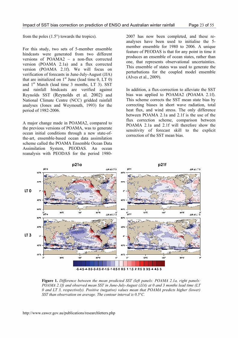
from the poles (1.5°) towards the tropics). For this study, two sets of 5-member ensemble hindcasts were generated from two different versions of POAMA2 – a non-flux corrected version (POAMA 2.1a) and a flux corrected version (POAMA 2.1f). We will focus on verification of forecasts in June-July-August (JJA) that are initialized on 1st June (lead time 0, LT 0) and 1st March (lead time 3 months, LT 3). SST and rainfall hindcasts are verified against Reynolds SST (Reynolds et al. 2002) and National Climate Centre (NCC) gridded rainfall analyses (Jones and Weymouth, 1993) for the period of 1982-2006. A major change made in POAMA2, compared to the previous versions of POAMA, was to generate ocean initial conditions through a new state-of-the-art, ensemble-based ocean data assimilation scheme called the POAMA Ensemble Ocean Data Assimilation System, PEODAS. An ocean reanalysis with PEODAS for the period 1980-
2007 has now been completed, and these re-analyses have been used to initialise the 5-member ensemble for 1980 to 2006. A unique feature of PEODAS is that for any point in time it produces an ensemble of ocean states, rather than one, that represents observational uncertainties. This ensemble of states was used to generate the perturbations for the coupled model ensemble (Alves et al., 2009). In addition, a flux-correction to alleviate the SST bias was applied to POAMA2 (POAMA 2.1f). This scheme corrects the SST mean state bias by correcting biases in short wave radiation, total heat flux, and wind stress. The only difference between POAMA 2.1a and 2.1f is the use of the flux correction scheme, comparison between POAMA 2.1a and 2.1f will therefore show the sensitivity of forecast skill to the explicit correction of the SST mean bias.
p21a p21f
Figure 1. Difference between the mean predicted SST (left panels: POAMA 2.1a, right panels: POAMA 2.1f) and observed mean SST in June-July-August (JJA) at 0 and 3 months lead time (LT 0 and LT 3, respectively). Positive (negative) values mean that POAMA predicts higher (lower) SST than observation on average. The contour interval is 0.5°C.
LT 0
LT 3

Impact of SST bias correction on prediction of ENSO and Australian winter rainfall Page 24 of 55
http://www.cawcr.gov.au/publications/researchletters.php
The resultant SST differences in the climate of the forecasts from the two different versions of POAMA2 and in the observed climate are displayed in Figure 1. As expected, the flux correction scheme reduces both the prominent cold and warm biases, with the cold bias across
the tropics now being less than 1.5°C and the warm bias off South America being reduced to less than 4°C (Figure 1 right panels).
(a) Standardized PCs
PC1
-4
-3
-2
-1
0
1
2
3
1982 1984 1986 1988 1990 1992 1994 1996 1998 2000 2002 2004 2006
Year
Sta
ndar
dize
d A
mpl
itude
PC2
-4
-3
-2
-1
0
1
2
3
1982 1984 1986 1988 1990 1992 1994 1996 1998 2000 2002 2004 2006
Year
Sta
ndar
dize
d A
mpl
itude
(b) Regression of SST anomaly on the PCs

Impact of SST bias correction on prediction of ENSO and Australian winter rainfall Page 25 of 55
http://www.cawcr.gov.au/publications/researchletters.php
(c) Regression of rainfall anomaly on the PCs
Figure 2. Dominant EOF modes of SST variability and the associated Australian rainfall component: (a) Standardized 1st (left panel) and 2nd (right panel) principal component time series (PCs) of tropical Indo-Pacific SST variability in JJA, (b) regression patterns of SST onto the standardized PCs, and (c) regression patterns of Australian rainfall onto the standardized PCs. The contour interval is 0.2°C per standard deviation of the respective PC in (b) and 0.1 mm per day per standard deviation of the respective PC in (c).
Observed relationship between ENSO and Australian rainfall in winter Prior to discussing the results of hindcasts from POAMA2 for the teleconnections of ENSO and Australian rainfall, the observed relationship between ENSO and rainfall in the last three decades is first reviewed. We begin by considering the relationship between the leading modes of tropical SST and rainfall. The leading modes of SST variability are identified with Empirical Orthogonal Function (EOF) analysis (North et al. 1982) over the domain of 30°S-20°N, 40°E -280°E. The spatial patterns of the first two EOF modes are displayed as the regression of SST anomaly onto the two leading principal component time series (PCs) and are scaled for a 1-standard deviation anomaly of the PCs (Figure 2a, b). Hereafter, these regression patterns are referred to as the EOFs. The spatial pattern of the first EOF mode represents canonical mature ENSO conditions (e.g. Trenberth, 1997), with maximum loading over the equatorial eastern Pacific (Figure 2b left panel). This mode explains 40% of the SST variance in winter. The second EOF mode (Figure 2b right panel) depicts east-west variations of each ENSO event (e.g. Trenberth and Stepaniak, 2000; Wang and Hendon, 2007). Previous studies have suggested
that El Niño events that have maximum warm SST anomaly over the central Pacific (i.e. events that have positive EOF2 in conjunction with positive EOF1; Trenberth and Stepaniak 2000, Ashok et al. 2007) tend to have more significant impact on regional climate over the Pacific rim countries (Hoerling and Kumar 2002, Kumar et al. 2006, Wang and Hendon 2007; Weng et al. 2007). EOF2 accounts for 18% of the total SST variance in austral winter, which is much less than EOF1 does, but because its loadings are located in the central Pacific in a region of warm background SST, changes in EOF2 can be associated with a large atmospheric response. The two leading modes of SST variability are both related to winter rainfall variability over eastern Australia (Figure 2c). SST EOF1 and EOF2 together can explain 20-40% of the total rainfall variance over the eastern states. However, the 2nd EOF of SST accounts for more winter rainfall variance than the first especially over Queensland and New South Wales. This finding is also confirmed by the stronger correlation of eastern Australian-mean rainfall (rainfall averaged over the land points east of 140°E) with SST PC2 (r ~ -0.5) than with SST PC1 (r ~ -0.3). Likewise, SST EOF2 explains more rainfall variance over the

Impact of SST bias correction on prediction of ENSO and Australian winter rainfall Page 26 of 55
http://www.cawcr.gov.au/publications/researchletters.php
western part of Western Australia than SST EOF1 does. Impact of reduced mean bias in SST on the predictions of ENSO and associated Australian rainfall In light of this updated understanding of different flavoured ENSO and its relationship with Australian rainfall in winter, we first assess how well POAMA simulates the spatial pattern of SST associated with the leading two modes of tropical SST. We do this by computing the spatial correlation (also called pattern correlation) between the observed and simulated leading modes of SST (Table 1). In POAMA 2.1a, the simulated EOF1 is more strongly correlated with the observed than is EOF2. And, while the correlation for both the first and second EOF drops off with increasing lead time, it drops off much quicker for EOF2. In the flux corrected version (POAMA 2.1f), both the initial pattern correlations are higher, and the drop off at longer lead time is reduced compared to the non-flux corrected version. This is an encouraging result that indicates a potentially significant benefit of reduction of mean-state bias for regional climate prediction: reduced bias in the ENSO mode should result in reduced bias in the ENSO teleconnection. We confirm this result after first assessing the impact of reduced mean state bias on prediction of ENSO.
Table 1. Pattern correlation of observed and predicted 1st and 2nd EOFs of tropical Pacific SST.
POAMA 2.1a LT 0 LT 3
EOF1 0.93 0.89
EOF2 0.84 0.66
POAMA 2.1f LT 0 LT 3
EOF1 0.95 0.91
EOF2 0.87 0.76
Assessment of the prediction of observed SST EOFs 1 and 2 was undertaken by projecting SST forecasts at all the grid points over the domain (30°S-20°N, 40°E -280°E) onto the observed EOF patterns shown in Figure 2, thus resulting in predictions of temporal loading coefficients (the
PCs). Skill is assessed using temporal correlation and normalized root-mean-squared-error (NRMSE; i.e., forecast RMSE normalized by the standard deviation of the corresponding observed PC time series). According to Figure 3, both non-bias corrected and bias corrected versions of POAMA2 can skillfully predict SST PC1 and PC2 up to a season in advance (correlation > 0.6 and NRMSE < 1). However, the effect of bias correction is not pronounced on the skill of predicting the variability of the observed leading pair of SST modes.
(a) Correlation PC1
0.5
0.6
0.7
0.8
0.9
1
LT0 LT3
Lead Time (months)C
orr.
Coe
ff.
p21ap21f
PC2
0.5
0.6
0.7
0.8
0.9
1
LT0 LT3
Lead Time (months)
Cor
r. C
oeff.
p21ap21f
(b) NRMSE
PC1
0
0.2
0.4
0.6
0.8
1
1.2
LT0 LT3
Lead Time (months)
Nor
mal
ized
RM
SE
p21ap21f
PC2
0
0.2
0.4
0.6
0.8
1
1.2
LT0 LT3
Lead Time (months)
Nor
mal
ized
RM
SE
p21ap21f
(c) Ratio of Spread to RMSE
PC1
0
0.2
0.4
0.6
0.8
1
LT0 LT3
Lead Time (months)
Spr
ead
to E
rror
Rat
io
p21ap21f
PC2
0
0.2
0.4
0.6
0.8
1
LT0 LT3
Lead Time (months)
Spre
ad to
Err
or R
atio
p21ap21f
Figure 3. (a) Correlation, (b) normalized root-mean-square-error (RMSE) of ensemble mean predictions and (c) ratio of ensemble spread to the RMSE of ensemble mean prediction of SST PC1 (left panels) and PC2 (right panels) from POAMA 2.1a (blue bars) and POAMA 2.1f (orange bars). The RMSE of each PC was normalized by the standard deviation of the observed counterpart (NRMSE). Bias correction appears to result in slight skill improvement in predicting EOF2 as demonstrated by reduced errors and increases in ensemble spread-to-error ratio, which is a positive sign because POAMA suffers from being overconfident (i.e. too low spread as indicated by small spread-to-error ratio), but there is an indication of reduced skill for EOF1 in the flux-corrected version at longer lead times.

Impact of SST bias correction on prediction of ENSO and Australian winter rainfall Page 27 of 55
http://www.cawcr.gov.au/publications/researchletters.php
(a) POAMA 2.1a LT 0 LT 3
(b) POAMA 2.1f LT 0 LT 3
Figure 4. Regression of predicted rainfall onto the predicted PCs of observed EOF1 and EOF2 in (a) POAMA 2.1a and (b) POAMA 2.1f. The contour interval is 0.1 mm per day per standard deviation of each PC time series
With regard to the simulation of the teleconnections between tropical Pacific SST and Australian rainfall, POAMA 2.1a, which is the non-flux corrected version, develops the wrong sign of teleconnection between the leading EOF of SST and eastern Australian rainfall at longer lead time: Although POAMA 2.1a simulates a realistic negative relationship between PC1 and Australian rainfall in the east at LT 0 (compare Figure 4a to Figure 2), the relationship erroneously changes sign by LT 3 (Figure 4a
upper panels). This error prevents POAMA from making skillful predictions of regional rainfall in Australia at longer lead time despite the ability to predict El Niño at longer lead time. In contrast, in POAMA 2.1f with bias correction, the erroneous teleconnection between PC1 and rainfall is much reduced, with the correct sign of the relationship now found in the far eastern side of the country at LT 3 (Figure 4b upper panels). Also, the stronger relationship of eastern Australian rainfall with PC2 than with PC1 in the observation is well represented at 3 month lead time in POAMA 2.1f but at the cost of losing the correct relationship between PC2 and rainfall over Western Australia. In summary, the flux corrected version of POAMA, while not providing significant skill improvement in predicting ENSO related SST variations, does better representing the teleconnection of El Niño to eastern Australian rainfall.
(a) POAMA 2.1a
LT 0 LT 3
(b) POAMA 2.1f LT 0 LT 3
Figure 5. Correlation of predicted rainfall in the non-flux corrected ((a); POAMA 2.1a) and flux corrected ((b); POAMA 2.1f) versions of POAMA2 with observed rainfall at lead time 0 and 3 months.
Our final question is, then, whether this improvement in teleconnection at longer lead time transfers to improved skill in predicting regional rainfall. Figure 5 displays correlation of rainfall predicted in POAMA 2.1a and POAMA 2.1f with observed rainfall. At LT 0, forecast skill of the

Impact of SST bias correction on prediction of ENSO and Australian winter rainfall Page 28 of 55
http://www.cawcr.gov.au/publications/researchletters.php
two versions is not very different to each other over most of Australia, but at LT 3 the flux corrected forecasts show much improved skill in eastern Australia. This is the region where the teleconnection to ENSO has been improved. Concluding remarks We have briefly re-examined the relationship between different types of ENSO events and Australian rainfall in the austral winter season and have investigated whether reduction of SST bias in the Bureau of Meteorology’s dynamical coupled seasonal forecast model can improve skill in predicting ENSO and simulating the teleconnections between ENSO and Australian rainfall. Observed Australian winter rainfall variability, especially over the east, is strongly associated with both traditional ENSO events that have peak SST anomaly in the eastern Pacific, and ENSO events that have peak SST anomaly in the central Pacific. In winter, a larger portion of eastern Australian rainfall variance is explained by the 2nd SST EOF whose maximum SST variability is located far westward of that of the 1st SST EOF. POAMA, even with substantial mean state SST bias and drift, can skillfully predict the first 2 observed EOF patterns of SST, but regional prediction of rainfall in eastern Australia is hindered at longer lead time because of an erroneous depiction of the teleconnection between eastern Pacific El Niño/La Niña events and rainfall at longer forecast lead time. This degradation of the teleconnection is attributed to the mean state drift in POAMA. Reduction of mean state bias via flux-correction does improve the model’s ability to simulate the leading two modes of tropical SST variability, but the skill in predicting the temporal evolution of the two leading modes of observed SST shows little sensitivity to bias correction. The improvement in depicting the spatial pattern of SST variability associated with the first two modes does carry over to an improved depiction of the teleconnection from ENSO and increased skill for predicting rainfall at longer lead time over eastern Australia. While not solving all the problems of predicting ENSO and its regional impacts in Australia, bias correction would appear
to be a viable solution for improving rainfall skill at longer lead time and should be considered as an option for implementation of POAMA2. Acknowledgements Support was provided by the South East Australian Climate Initiative. The authors are grateful to Drs Li Shi and Harun Rashid for their useful comments on the manuscript. References Ashok, K., S. K. Behera, S. A. Rao, and H. Weng, 2007: El Niño Modoki and its possible teleconnection. Journal of Geophysical Research, 112, C1107, doi:10.1029/2006JC003 798. Alves, O., H. Hendon, G. Wang, Y. Yin, E. Lim and D. Hudson 2009: Report on skill of direct rainfall and temperature forecasts from the new generation national dynamical forecast model. SEACI final report for Project 3.1.4. Drosdowsky, W. and L. Chambers, 2001: Near-global sea surface temperature anomalies as predictors of Australian seasonal rainfall. Journal of Climate, 14, 1677-1687. Hendon, H. H., E. Lim, G. Liu, and O. Alves 2007: Assessment of simulation by POAMA of modes of climate variability that drive rainfall in SE Australia. SEACI Technical Report, Milestone 3.1.3. Hendon, H. H., E. Lim, G. Wang, O. ALves, and D. Hudson, 2009: Prospects for predicting two flavors of El Nino. Geophysical Research Letters, 36, L19713, doi:10.1029/2009GL040100 Hoerling, M.P. and A. Kumar, M. Zhong 1997: El Niño, La Niña, and the Nonlinearity of Their Teleconnections. Journal of Climate 10, 1769–1786. Jones, D. A. and G. Weymouth, 1997: An Australian monthly rainfall dataset. Technical Report 70, Bureau of Meteorology. Kumar K. K., B. Rajagopalan, M. Hoerling, G. Bates, and M. Cane, 2006: Unraveling the mystery of Indian monsoon failure during El Niño. Science, 314, 115–119. Lim, E.-P., H. H. Hendon, and O. Alves, 2009a: Intercomparison of seasonal forecast models for South Eastern Australian Climate. SEACI final report for project 3.1.2. Lim, E.-P., H. H. Hendon, D. Hudson, G. Wang and O. Alves 2009b: Dynamical forecast of inter-El Niño variations of tropical SST and Australian spring rainfall, Monthly Weather Review, 137, 3796-3810. McBride, J. L. and N. Nicholls 1983: Seasonal relationships between Australian rainfall and the Southern Oscillation. Monthly Weather Review, 111, 1998–2004. North, G. R., T. L. Bell and R. F. Cahalan, 1982: Sampling

Impact of SST bias correction on prediction of ENSO and Australian winter rainfall Page 29 of 55
http://www.cawcr.gov.au/publications/researchletters.php
errors in the Estimation of Empirical Orthogonal Functions. Monthly Weather Review, 110, 699-706. Reynolds, R. W., N. A. Rayner, T. M. Smith, D. C. Stokes, and W. Wang, 2002: An improved in situ and satellite SST analysis for climate. Journal of Climate, 15, 1609–1625. Schiller, A., J. S. Godfrey, P. C. McIntosh, G. Meyers, N. R. Smith, O. Alves, G. Wang, and R. Fiedler, 2002: A New Version of the Australian Community Ocean Model for Seasonal Climate Prediction. CSIRO Marine Research Report No. 240, 82 pp. Trenberth, K. E., 1997: The definition of El Niño. Bulletin of the American Meteorlogical Society, 78, 2771–2777. Trenberth, K. E. and D. P. Stepaniak, 2001: Indices of El Niño evolution. Journal of Climate, 14, 1697–1701.
Wang, G. and H. H. Hendon, 2007: Sensitivity of Australian rainfall to inter-El Niño variations. Journal of Climate, 20, 4211-4226. Wang, G., O. Alves, D. Hudson, H. Hendon, G. Liu, and F. Tseitkin, 2008: SST Skill assessment from the new POAMA-1.5 system. BMRC Research Letters, 8, 1–6. Weng H., K. Ashok, S. K. Behera, S. A. Rao, and T. Yamagata, 2007: Impacts of recent El Niño Modoki on dry/wet conditions in the Pacific Rim during boreal summer. Climate Dynamics, 29, 113–129. Zhong, A., H. H. Hendon and O. Alves., 2005: Indian Ocean variability and its association with ENSO in a Global Coupled Model. Journal of Climate, 18, 3634-3649.

Short-Term Variability of Ozone and UV: a case study Page 30 of 55
http://www.cawcr.gov.au/publications/researchletters.php
Short-Term Variability of Ozone and UV: A case study L. L. Lemus-DeschampsA, T. HumeB and N. MoodieC
ABCAWCR, Bureau of Meteorology CWeather Services Branch, Bureau of Meteorology
Introduction There is a general perception in the Australian community that surface ultraviolet radiation (UV) does not change significantly from day to day. However, the impact of synoptic weather systems on total ozone amount has been known for several decades. The relationship between ozone and UV is also well defined, where, in the absence of clouds, ozone decreases lead to increases in ultraviolet radiation (UV) levels at the surface. The perception within the community is that clear-sky UV Index changes are smooth and small from day to day, with month to month changes more easily noticed than the daily values. Here we illustrate that daily changes in clear-sky UV radiation strongly depend on the short term ozone variability, which is related to the passage of weather systems. The Bureau of Meteorology issues daily UV Index forecasts (Lemus-Deschamps et al. 1999, 2004, 2006). The UV Index forecast is used in Cancer Council Australia’s sun-protection educational and promotional campaigns. The main factors that affect the amount of UV radiation reaching the Earth’s surface are ozone, geographical location, Rayleigh scattering, aerosols, surface albedo, clouds, time of day and day of the year. Geographical location and the time of day, and day of the year determine the solar zenith angle. Large solar zenith angle and reduced amount of atmospheric absorption/scattering corresponds to higher surface UV levels. UV radiation levels peak at solar noon time during summer. The Bureau of Meteorology produces operational forecasts of clear-sky UV valid at local noon (http://www.bom.gov.au/weather/uv/). The UV forecast model takes into account the factors described above, and also meteorological information from the Bureau’s Global Assimilation and Prediction System. The clear-
sky UV radiation is then weighted by the erythemal spectral response of human skin from the Commision Internationale d’Eclairage (CIE, 1987), integrated over the 290-400 nm wavelength interval every 1 nm. This produces the “erythemal-dose-rate”, which is published as the standard ultraviolet radiation index (UV Index), where one UV Index unit is equal to 25 mW/m2 (WMO, 1995; WHO, 2002). The UV Index is a numerical value with a descriptive danger category; values below 3 are considered low, between 3 to 5 moderate, between 6 to 7 high, between 8 to 10 very high, and 11 or above are considered extreme. A UV Alert is issued when the UV Index forecast is three or above. UV and ozone forecasts are continuously verified against satellite and surface measurements (Lemus-Deschamps et al. 2004; Gies et al. 2004).
Ozone and UV Index variability The total ozone amount, which is required to compute the UV Index, is calculated by assimilation of satellite radiances and GASP meteorological fields. It is assumed that most of the ozone lies in a layer between the 375K isentrope (near the tropopause) and the top of the model. This layer is advected using the forecast isentropic wind and pressure thickness from GASP (Grainger, 1998; Atking et al. 1997; Lemus-Dechamps et al. 1999, 2004, 2006; Deschamps et al. 2006a). Stratospheric ozone (between 15 and 50 km) absorbs almost all UV below 300 nm. However, only a fraction of UV radiation above 300 nm is absorbed by the ozone. If all other environmental factors are kept constant, reduced stratospheric ozone leads to increased surface UV radiation. This is illustrated in Figure 1 where the 1980 to 2007 summer mean total ozone and UV Index for Melbourne (37.48S, 144.58E) are presented. Total ozone in Dobson Units (DU) is proportional to the pressure-weighted vertical integral of ozone mixing ratio profile.

Short-Term Variability of Ozone and UV: a case study Page 31 of 55
http://www.cawcr.gov.au/publications/researchletters.php
Figure1. Melbourne, summer total ozone (DU) from TOMS/OMI satellite data and UV Index calculated from assimilation of TOMS/OMI total ozone into the BoM’s UV radiation model.
Lower total ozone concentrations are found in the tropics than in the high latitudes, largely as a result of the Dobson-Brewer circulation. In the tropics mean upward motion raises ozone-poor air from lower levels, and transports high level ozone-rich air pole-ward. The pole-ward transport in the winter hemisphere contributes to the ozone maximum there. The amplitude of the seasonal ozone cycle varies substantially with latitude. At the tropics smaller seasonal variation is observed, intensifying towards middle and high latitudes, with ozone maximum usually observed at most extra-tropical latitudes during spring. At high southern latitudes the strongest westerly winds occur during the winter. These winds isolate the Antarctic region where a total ozone minimum is observed due to the onset of significant springtime stratospheric ozone depletion. Examples illustrating the seasonal variation of total ozone for Alice Springs (23.40S, 133.5E) and Melbourne (37.48S, 144.58E) during 2008 and 2009 are presented in Figure 2a and 2b (top panel). The corresponding UV Index is also presented in the bottom panel of Figure 2a and 2b. At the peak of summer and winter lower maximum levels of UV Index are observed for Melbourne than for Alice Springs. This is mainly driven by the solar zenith angle difference between Alice Springs and Melbourne.
Changes in stratospheric ozone, due to transport from the equatorial source region during the winter and spring, regulates the seasonal variance of the extra-tropical total ozone. At shorter time scales (a day to a few days), most ozone variability is caused by the passage of tropospheric weather systems. These systems can impact the vertical and horizontal transport of lower stratospheric air. Dobson et al. (1929, 1968) showed that there is a connection between synoptic meteorological disturbances and ozone column amounts. They reported that synoptic weather systems impact the flow above and below the tropopause, with increases in total ozone values connected to the passage of cold fronts and decreases to warm fronts, and high total ozone values are found to the rear of developing tropospheric cyclones and low total ozone values are found at surface anti-cyclones. Reed (1950) showed that vertical motions in the lower stratosphere associated with trough/ridge patterns produce most of the short term variance in total ozone. Air parcels above the tropopause, that are affected by weather systems, will stretch in a trough and compress in a ridge. To maintain mass continuity, the horizontal divergence and convergence results in integrated total ozone values, that are larger in sinking motions and smaller in upward motions. Ozone displaced downward undergoes compression increasing the column abundance (high ozone) in that region, while ozone displaced upwards undergoes expansion decreasing the column abundance (low ozone). Day to day changes in ozone and UV Index levels are illustrated for Melbourne and Alice Springs in Figure 2. Even though the amplitude of ozone variability tends to be smaller during winter than summer, the impact on UV Index is still noticeable. Melbourne exhibits a larger day to day variability than Alice Springs during spring and summer.
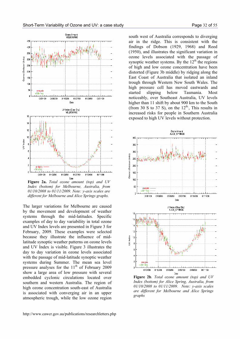
Short-Term Variability of Ozone and UV: a case study Page 32 of 55
http://www.cawcr.gov.au/publications/researchletters.php
Figure 2a. Total ozone amount (top) and UV Index (bottom) for Melbourne, Australia, from 01/10/2008 to 01/11/2009. Note: y-axis scales are different for Melbourne and Alice Springs graphs.
The larger variations for Melbourne are caused by the movement and development of weather systems through the mid-latitudes. Specific examples of day to day variability in total ozone and UV Index levels are presented in Figure 3 for February, 2009. These examples were selected because they illustrate the influence of mid-latitude synoptic weather patterns on ozone levels and UV Index is visible. Figure 3 illustrates the day to day variation in ozone levels associated with the passage of mid-latitude synoptic weather systems during Summer. The mean sea level pressure analyses for the 11th of February 2009 show a large area of low pressure with several embedded cyclonic circulations located over southern and western Australia. The region of high ozone concentration south-east of Australia is associated with converging air in an upper atmospheric trough, while the low ozone region
south west of Australia corresponds to diverging air in the ridge. This is consistent with the findings of Dobson (1929, 1968) and Reed (1950), and illustrates the significant variation in ozone levels associated with the passage of synoptic weather systems. By the 12th the regions of high and low ozone concentration have been distorted (Figure 3b middle) by ridging along the East Coast of Australia that isolated an inland trough through Western New South Wales. The high pressure cell has moved eastwards and started slipping below Tasmania. Most noticeably, over Southeast Australia, UV levels higher than 11 shift by about 900 km to the South (from 30 S to 37 S), on the 12th., This results in increased risks for people in Southern Australia exposed to high UV levels without protection.
Figure 2b. Total ozone amount (top) and UV Index (bottom) for Alice Spring, Australia, from 01/10/2008 to 01/11/2009. Note: y-axis scales are different for Melbourne and Alice Springs graphs

Short-Term Variability of Ozone and UV: a case study Page 33 of 55
http://www.cawcr.gov.au/publications/researchletters.php
Figure 3a. Bureau of Meteorology’s Australia UV Index (top), total ozone amount (middle) forecast and (bottom) Australia mean sea level pressure, (MSLP) for 11/02/2009
Figure 3b. Bureau of Meteorology’s Australia UV Index (top), total ozone amount (middle), forecast and (bottom) Australia mean sea level pressure (MSLP) for 12/02/2009.
Conclusions The examples above demonstrate that day to day UV index levels are affected by the passage of synoptic weather systems, particularly during the spring and summer. Variations of UV caused by ozone variability are also observed during winter,
but their magnitude is smaller than during the summer. Large fluctuations in UV index levels may become problematic for public health agencies charged with promoting the sun safe message in the community. Sun safe messages work effectively when they are simple and easily

Short-Term Variability of Ozone and UV: a case study Page 34 of 55
http://www.cawcr.gov.au/publications/researchletters.php
understood by the community. However, as demonstrated by this case study, during the Southern Hemisphere Summer the UV index can oscillate between the High and Extreme categories for areas of Southern Australia. Even though the response levels required of the community are the same for both categories, the impact of excessive exposure to the Sun increases substantially as the UV index reaches deep into the Extreme category. Thus, the challenge for awareness campaigns is to overcome any complacency that builds within the community during summer, by highlighting the risks of excess sun exposure on a day to day basis through promotion of the daily UV Index forecast provided by the Bureau of Meteorology.
References Atkinson, R., S. Grainger and P.M. Udelhofen, 1997: A scheme for the routine analysis and deterministic prediction of the global total ozone distribution: Proceedings of AMS International Conference on the Meteorology of the Southern Hemisphere, Pretoria, Africa.
Dobson, G.M.B., D.N. Harrison and J. Lawrence, 1929: Measurements of the amount of ozone in the earth’s atmosphere and its relation to other geophysical conditions: Part III, Proc. R. Soc. London, A122, 456-458.
Dobson, G., 1968: Exploring the Atmosphere, 209pp, Claredon, Oxford.
Gies, P.,Colin Roy, John Javorniczky, Stuart Henderson, Lilia Lemus-Deschamps, and Colin Driscoll, 2004: Global Solar UV Index: Australian Measurements, Forecasts and Comparison with the UK. Photochem.Photobiol.79(1), 32-39.
Grainger, S., 1998: Global analysis of ozone by statistical interpolation of satellite data. PhD Thesis, 182pp, Monash University, Melbourne Australia. Commision Internationale d’Eclairage., 1987. A reference action spectrum for ultraviolet induced erythema in human skin, C.I.E. Journal, 6, 17-22. Lemus-Deschamps, L., P. Gies, L. Rikus, K. Strong and H. Dixon, 2006, UV Index: Forecasts and Media Weather Reports. UV Radiation and its Effects, Report of the NIWA Workshop, Dunedin, New Zealand, April 2006. RSNZ, Miscellaneous series, 68, 25-26. Deschamps L., P. Gies, L. Rikus, R. Dare and K. Strong, 2006a, UV Index for Sun Safety. BMRC Research Letters, 4, 34-35 Lemus-Deschamps, L., L. Rikus, S.Grainger, P. Gies, J. Sisson and Z. Li, 2004: UV Index and UV dose distributions for Australia (1997-2001). Australian Meteorological Magazine, 53, 239-250. Lemus-Deschamps, L., L. Rikus and P. Gies, 1999: The operational Australian ultraviolet index forecast 1997. Meteorological Applications, 6, 241-251. Reed, R.J., 1950: The role of vertical motions in ozone-weather relationships, Journal of Meteorology, 7, 263-267, 1950. WHO, 2002: Global Solar UV Index, A practical Guide. Fact Sheet 271. http://www.who.int/mediacentre/factsheet/who271/en/index.html. WMO, 1995: Panel Report of the WMO Meeting of Experts on UV-B measurements, Data Quality and Standardization of UV Indices. WMO/TD No.625.

Surface energy balance in ACCESS: comparisons with observation based fluxes Page 35 of 55
http://www.cawcr.gov.au/publications/researchletters.php
Surface energy balance in the ACCESS models: comparisons with observation based flux products
Harun A. RashidA, Martin DixB, and Anthony C. HirstC ABCCentre for Australian Weather and Climate Research
CSIRO Marine and Atmospheric Research
Private Bag 1, Aspendale, VIC 3195, Australia
Introduction The Australian Community Climate and Earth System Simulator (ACCESS) is a fully coupled modelling system being developed by CAWCR and participating Australian universities. The atmospheric component of this coupled modelling system will be a state-of-the-art atmospheric GCM (AGCM) based on the UK Met Office unified model (UM). As this AGCM constitutes the atmospheric component of the ACCESS coupled model, it is important that the simulated surface energy fluxes compare favourably with those derived from observations. In particular, diagnostics such as the global integral of the net heat flux at the air-sea interface and the meridional ocean heat transports implied by this flux can provide an indication of the possible coupled model behaviour. The ACCESS coupled modelling team is currently evaluating options for the version of the UM AGCM to be used for the initial ACCESS coupled model system. In this work, we investigate the realism of the surface energy flux in four multi-decadal simulations of the UM AGCM, two performed by the ACCESS team at CAWCR and two performed at the Hadley Centre of the MetOffice (HCMO).. The simulated energy balance is validated against the observation-based surface flux products CORE version 2 (hereafter, CORE.v2; Large and Yeager 2009). We also compare these results with similar results derived from a coupled model simulation recently performed at the UK Met Office.
Traditionally, the net heat flux and the implied meridional oceanic heat transport (IMOHT) have been used to indirectly estimate the oceanic heat transport from the measurement of atmospheric fluxes at the top-of-atmosphere or at the surface (e.g., Carissimo et al. 1985; Hsiung 1985; Trenberth and Caron 2001). However, many
recent studies have also used these diagnostics for the analysis and validation of atmospheric model performance (e.g., Gleckler et al. 1995; Hack 1998; Gleckler 2005). If the AGCM simulated net heat fluxes, and therefore the IMOHT, are significantly different from the observations, then the AGCM is likely to contribute to the climate drift if used as the atmospheric component of a coupled model. Comparing the geographical distribution of the simulated net heat flux with that of the observed allows us to uncover important model biases, the origins of which may then be traced back to, e.g., different physical parameterisation schemes used in the model. The end result of such exercises may well be improved model performances brought about through improvements in physical parameterisations. Therefore, our intention here is to examine the aforementioned diagnostics from several simulations across three different UM AGCM model versions, to help determine the versions’ relative suitability for being used as the atmospheric component of the coupled model. We will also briefly discuss the possible origin of bias seen in one of the dominant components of the net heat flux, namely the shortwave flux.
In the following section, a brief description of the AGCM is given and the validation dataset is also described. The subsequent section describes the model experiments, the simulated net surface heat flux and the IMOHT. We summarise the main conclusions of this study in a final section.
Model and validation dataset The AGCM configurations used in this study have N96 horizontal resolution, equivalent to a 1.25○ by 1.875○ latitude–longitude grid. There are 38 levels in the vertical, with the top level placed
Surface energy balance in ACCESS: comparisons with observation based fluxes Page 36 of 55
http://www.cawcr.gov.au/publications/researchletters.php
at a height of about 40 km. The AGCM has a non-hydrostatic dynamical core, and includes a comprehensive set of sophisticated parameterization schemes for physical processes. Among the parameterized physical processes are radiation and ozone, interactive aerosols, land surface processes and hydrology, boundary layer turbulent mixing, convection, cloud and precipitation microphysics, and gravity wave drag. A more complete description of the model is given in Johns et al. (2006).
Three versions of the AGCM are featured here. The first version is the CAWCR implementation of HadGEM1a-A, though this implementation includes the new prognostic cloud fraction and prognostic condensate scheme (PC2) (Wilson et al. 2008), instead of the standard scheme of Smith (1990). PC2 calculates increments to prognostic variables of liquid, ice and total cloud fractions, water vapour and liquid condensate as a result of each physical process represented in the model. This version is referred to as “HadGEM1a-A+PC2”. The second version is that of the standard HadGEM2-A (Collins et al. 2008) and this uses the Smith (1990) cloud scheme. The third version is a prototype version of HadGEM3-A (the March 2009 assessment)1. The prototype is developed from HadGEM2-A and includes the following changes: PC2 cloud scheme, van Genuchten (1980) soil hydraulics, increased CAPE closure timescale for convection (UM Documentation paper no 27 "Convection scheme") with facility to shorten this timescale in cases of high vertical velocity, improved land surface hydrology scheme, CLASSIC soil albedos, and numerous other minor changes.
The validation dataset is based on a recent version of the CORE flux products, CORE.v2 (Large and Yeager 2009). The air-sea fluxes of momentum, heat, freshwater and their components were computed over the period 1948–2006 using the bulk formulas. The input data were based on NCEP reanalysis (Kalnay et al. 1996), which were used in the bulk formulas after making some adjustments against high-quality satellite and in-situ observations. The radiative fluxes were based on ISCCP (International Satellite Cloud Climatology 1Note that HadGEM3 is still under development and the present configuration does not represent the final version
Project) products (Zhang et al. 2004). The result of these adjustments was an improved global mean balance, reducing, for example, the climatological global mean heat flux from 30 Wm-2 to 2 Wm-2. Here, we use the net heat flux and its components—net shortwave flux (SW), net longwave flux (LW), latent heat flux (LH) and sensible heat flux (SH)—for validation of the simulated fluxes. While monthly varying LH and SH are available for the entire period (1948–2006), the monthly varying radiative heat fluxes (SW and LW) are available only since 1984. Therefore, CORE.v2 data for the period 1984–2006 are used in the evaluations.
Model experiments The simulations featured in this study are detailed in Table 1. These include four AGCM simulations and one coupled model simulation. The AGCM simulations are performed according to an AMIP-style protocol, namely using the monthly varying sea surface temperature (SST) and sea-ice distributions2 for the periods indicated in Table 1. Additional atmospheric forcings were used as summarised in Table 1. Two of the four AGCM simulations were performed locally at CAWCR as part of the ACCESS model development efforts, and the other simulations (two AGCM and one coupled) were performed at the Met Office. The model simulations come with different integration lengths and periods. Where possible, data records of the same period as for CORE.v2 have been used. All results are based on long-term means of the flux diagnostics, so slight differences in run length or period do not affect our results in any significant way. Note that the simulation years for the coupled run are arbitrary and do not correspond to any specific range of calendar years, except that forcing conditions are for the present-day.
The coupled model simulation uses HadGEM3-AO (March 2009 assessment) and has the same atmosphere as the HadGEM3-A simulation analysed here. The other components of this coupled model include the NEMO ocean model, the CICE sea ice model, and the OASIS coupler. 2 The SST and sea ice fields are obtained from PCMDI, including updates to 2008 in the case of the CAWCR simulations..
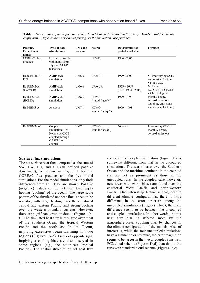
Surface energy balance in ACCESS: comparisons with observation based fluxes Page 37 of 55
http://www.cawcr.gov.au/publications/researchletters.php
Table 1. Descriptions of uncoupled and coupled model simulations used in this study. Details about the climate configuration, type, source, period and forcings of the simulations are provided.
Product/ Experiment names
Type of data /simulations
UM code version
Source Data/simulation period available
Forcings
CORE.v2 Flux products
Use bulk formula, with inputs from adjusted NCEP reanalyses
NCAR 1984 - 2006
HadGEM1a-A + PC2
AMIP-style simulation
UM6.3 CAWCR 1979 - 2000
HadGEM2-A (CAWCR)
AMIP-style simulation
UM6.6 CAWCR 1979 – 2008 (used: 1984– 2006)
HadGEM2-A (HCMO)
AMIP-style simulation
UM6.6 HCMO (run id “ageyb”)
1979 - 1998
HadGEM3-A As above UM7.1 HCMO (run id “ahrqc”)
1979 - 1998
Time varying SSTs and sea-ice fraction Fixed CO2,
Methane, N2O,CFC11,CFC12 Climatological
monthy ozone, aerosol emissions (sulphate emissions include secular trend)
HadGEM3-AO Coupled simulation; UM, Nemo and CICE coupled through OASIS flux coupler
UM7.1 HCMO (run id “ahsaf”)
30 years Present-day GHGs, monthly ozone, aerosol emissions
Surface flux simulations The net surface heat flux, computed as the sum of SW, LW, LH, and SH (all defined positive downward), is shown in Figure 1 for the CORE.v2 flux products and the five model simulations. For the model simulations, only their differences from CORE.v2 are shown. Positive (negative) values of the net heat flux imply heating (cooling) of the ocean. The large scale pattern of the simulated net heat flux is seen to be realistic, with large heating over the equatorial central and eastern Pacific and strong cooling over the western boundary currents. However, there are significant errors in details (Figures 1b–f). The simulated heat flux is too large over most of the Southern Ocean, the tropical Western Pacific and the north-east Indian Ocean, implying excessive ocean warming in those regions (Figures 1b–e). Errors of opposite sign, implying a cooling bias, are also observed in some regions (e.g., the south-east tropical Pacific). The spatial structure of net heat flux
errors in the coupled simulation (Figure 1f) is somewhat different from that in the uncoupled simulations. The warm biases over the Southern Ocean and the maritime continent in the coupled run are not as prominent as those in the uncoupled runs. In the coupled case, however, new areas with warm biases are found over the equatorial West Pacific and north-western Pacific. One interesting feature is that, despite different climate configurations, there is little difference in the error structure among the uncoupled simulations (Figures 1b–e); the main difference seems to be between the uncoupled and coupled simulations. In other words, the net heat flux bias is affected more by the atmosphere-ocean coupling than by changes in the climate configuration of the models. Also of interest is, while the four uncoupled simulations have a similar error structure, the error magnitude seems to be larger in the two uncoupled runs with PC2 cloud scheme (Figures 1b,d) than that in the runs with standard cloud scheme (Figures 1c,e).

Surface energy balance in ACCESS: comparisons with observation based fluxes Page 38 of 55
http://www.cawcr.gov.au/publications/researchletters.php
Figure 1. Geographical distributions of the net heat flux (Wm-2) into the ocean for a) CORE.v2 flux products, b) HadGEM1a-A+PC2 minus CORE.v2, c) HadGEM2-A (CAWCR) minus CORE.v2, d) HadGEM3-A minus CORE.v2, e) HadGEM2-A (HCMO) minus CORE.v2, and f) HadGEM3-AO minus CORE.v2.
The long-term, global mean heat balance is an important diagnostic, which may be indicative of the presence (or absence) of climate drift in coupled simulations. The global ocean-area averages of the net heat flux derived from CORE.v2 and the five model simulations are shown in Table 2. For CORE.v2, the average net heat flux into the ocean is 2 Wm-2. This positive imbalance is consistent with the observed 20th century warming of the global oceans (Levitus et al. 2005; Domingues et al. 2008). The modelled
ocean-mean values are similar to observed values, but with some differences. One of the uncoupled models that uses the PC2 cloud scheme, HadGEM1a-A+PC2, shows the largest net heat flux balance (3.12 Wm-2). The smallest ocean-mean value (1.38 Wm-2) occurs for the HadGEM2-A (CAWCR) run, whereas somewhat larger than observed values (2.12 and 2.24 Wm-2) occur for the two uncoupled runs from the Met Office (Table 2).

Surface energy balance in ACCESS: comparisons with observation based fluxes Page 39 of 55
http://www.cawcr.gov.au/publications/researchletters.php
Figure 2. Geographical distributions of the bias in HadGEM2-A (CAWCR) simulation of a) downward shortwave radiation (Wm-2) at the surface and b) shortwave cloud radiative forcing (Wm-2) at the surface. The cloud radiative forcing is computed as the difference between the all-sky and clear shortwave radiations at the surface. The observed data for all-sky and clear shortwave radiations are available from the ISCCP-FD dataset for the period 1984–2000, and simulated data for the same period were used in the calculations for this Figure
The ocean-mean value simulated by the Met Office coupled model (1.97 Wm-2) is very close to that observed. The difference between the pair of coupled and uncoupled models, HadGEM3-A and HadGEM3-AO, indicates the correction that occurs in ocean-mean net heat flux due to
coupling, i.e., the allowance of air-sea interactions. Also, the difference between the ocean-mean net heat fluxes simulated by the two uncoupled models using the same cloud scheme, HadGEM2-A (CAWCR) and HadGEM2-A (HCMO), is mostly due to the different

Surface energy balance in ACCESS: comparisons with observation based fluxes Page 40 of 55
http://www.cawcr.gov.au/publications/researchletters.php
simulation lengths and computing platforms.
Table 2. Global ocean-area averaged net heat flux imbalances (Wm-2) computed from the CORE.v2 flux products and the model simulations.
Product/Experiment names Global ocean averaged
net heat flux (Wm-2) CORE.v2 1.99 HadGEM2-A (CAWCR) 1.38 HadGEM1a-A +PC2 3.12 HadGEM3-A 2.24 HadGEM2-A (HCMO) 2.12 HadGEM3-AO 1.97
An examination of the component fluxes (not shown) shows that the main contributions to the net surface heat flux errors come from the net shortwave flux and latent heat flux, which are responsible, on average, for the excessive (implied) ocean warming and cooling, respectively. To better understand the nature of the shortwave flux error, we computed the shortwave cloud radiative forcings (CRFs) from the HadGEM2-A (CAWCR) simulation and the ISCCP-FD dataset (Zhang et al. 2004). The shortwave CRF was computed as the difference of downward shortwave radiations at the surface under the all-sky and clear-sky conditions (Ramanathan et al. 1989). The shortwave CRF is in general a negative quantity, indicating the cooling effect of clouds due to blocking of the shortwave radiation. Figure 2 shows the difference between the modelled and observed shortwave CRFs (Figure 2b), along with a similar difference in downward shortwave fluxes at the surface (Figure 2a). A comparison between these two Figures immediately shows a close resemblance between the spatial structures of the shortwave flux error and the shortwave CRF error, except over the North Pacific. It is therefore clear that the modelled shortwave flux errors over most of the global oceans occur due to the erroneous simulation of the cloud radiative effects by the AGCM.
Implied meridional ocean heat transports From the consideration of energy conservation, the net surface heat flux into the ocean implies a divergence/convergence of the vertically
integrated oceanic heat transports. This assumes that the time-mean ocean mixed layer temperatures remain constant, when the mean is computed from a sufficiently long data record. In case of the zonally-averaged net heat flux, the implied oceanic heat transport is in the meridional direction, which can be readily computed as
θθθπθθ
π
dFaIMOHT s cos)(2)(2/
2 ∫−
=
where, θ is latitude, Fs is the time- and zonally- averaged net heat flux at the air-sea interface, and a is Earth’s radius. We computed the IMOHT separately for the three ocean basins (Pacific, Atlantic and Indian Oceans), as well as for the global ocean as the sum of the contributions from these ocean basins3. Before the computation we subtracted the respective global ocean-area averages (Table 2) from the observed and simulated net heat fluxes. The results for the CORE.v2 products and the model simulations are shown in Figure 3. The IMOHT in the simulation and CORE.v2 flux products are in reasonable agreement, with mostly poleward heat transports in both Hemispheres (with the exception of a small northward transport in Southern mid-latitudes). Among the three ocean basins the Pacific and Atlantic Oceans are the main contributors to the total IMOHT (Figure 3a). In the Northern Hemisphere the total transport consists of the contributions by these two oceans, with the Atlantic Ocean transporting somewhat more than the Pacific. In the Southern Hemisphere, the Atlantic and Pacific Oceans counteract each other, with the former (latter)
3 Note that there is water (and heat) exchange between the Indian and Pacific at 8°S and between the Atlantic and Indian at 35°S. Therefore, the “IMOHT” calculated southward of these latitudes for the separate ocean basins (8°S for the Pacific and Indian, 35°S for the Atlantic) continues to represent a surface flux integral meaningful for comparison, but would not correspond with the actual meridional ocean heat transport in the separate basins.

Surface energy balance in ACCESS: comparisons with observation based fluxes Page 41 of 55
http://www.cawcr.gov.au/publications/researchletters.php
Figure 3. The implied meridional oceanic heat transports (PW), computed from the net heat flux into the ocean, for a) CORE.v2 flux products, b) HadGEM1a-A+PC2, c) HadGEM2-A (CAWCR), d) HadGEM3-A, e) HadGEM2-A (HCMO), and f) HadGEM3-AO.
Surface energy balance in ACCESS: comparisons with observation based fluxes Page 42 of 55
http://www.cawcr.gov.au/publications/researchletters.php
transporting heat northward (southward). The Indian Ocean contribution is small and has opposite signs in the Southern subtropics and extratropics.
While there are agreements between the observed and simulated IMOHTs, significant differences are found between them and, also, among the simulated IMOHTs. The most notable disagreement is found over the Southern mid-latitudes, where the uncoupled models show large northward transports (Figures 3b–e). This bias, however, mostly disappears in the coupled simulation (Figures 3f), suggesting that the IMOHT bias in the uncoupled runs arises, at least in part, because of the artificial suppression of atmosphere–ocean interactions in these runs. Differences in the experiment setup (i.e., climate configuration, including the cloud scheme) can also contribute significantly to the IMOHT bias (cf. Figures 3c,d).
Conclusions In this paper, we have examined the net surface heat flux and related diagnostics in long-term simulations with several uncoupled and coupled models. The realism of the simulated net heat flux and the IMOHT has been assessed by comparing these diagnostics with those derived from the CORE.v2 flux products. The atmospheric GCM used in the uncoupled and coupled simulations is based on various recent versions of the UM. One main objective of this study is to determine the readiness of the atmospheric GCM for long coupled model simulations. Our results show that the large scale patterns of the simulated and observed (i.e., observation-based flux products) net surface heat fluxes compare favourably with each other. However, there are some significant differences in details of the simulated and observed fluxes. In particular, the AGCM simulates excessive net surface heat flux into most of the Southern Ocean, and into the tropical Western Pacific and the north-east Indian Ocean. There are also regions, e.g., the south-east tropical Pacific, where the simulated net surface flux into the ocean is less than the observed. The main contributions to these net surface flux errors come from net shortwave flux and latent heat flux components. The AGCM
simulates too much net shortwave flux (implying erroneous local warming of the ocean) and latent heat flux (i.e., erroneous local cooling of the ocean). The bias in the shortwave flux is found to be associated with erroneous representations of the cloud radiative forcing in the model. The IMOHTs for the individual ocean basins also show realistic meridional profiles, except for the Southern mid-latitudes. In this latter region, the observed IMOHT shows near zero or southward transports, whereas the simulated IMOHT shows large northward transports, especially in the uncoupled simulations. These errors in the uncoupled simulations, however, mostly disappear in the coupled simulation. This suggests that the IMOHT errors in the uncoupled models arise, for the most part, due to the artificial suppression of coupled air-sea interactions. However, a more detailed examination of the coupled model simulation will be needed to determine whether or not other model biases have developed to create compensations. We, however, emphasize that the AGCM is still deficient in many respects (only a few of which are discussed in this paper), and is likely to contribute along with other component models to the numerous deficiencies commonly observed in coupled model simulations. Therefore, the ongoing development of the AGCM, especially the parameterizations of physical processes, needs to be continued for improved realism of both uncoupled and coupled simulations.
Acknowledgements We acknowledge the contributions made by the members of the ACCESS coupled modeling team. Thanks are due to Dr. Gill Martin of the Hadley Centre (UK Met Office) for providing simulation data from the Met Office model runs. References Carissimo, B. C., A. H. Oort, and T. H. Vonder Haar, 1985: Estimating the meridional energy transports in the atmosphere and ocean. Journal of Physical Oceanography, 15, 82-91. Collins, W. J., N. Bellouin, M. Doutriaux-Boucher, N. Gedney, T. Hinton, C.D. Jones, Liddicoat, G. Martin, F. O’Connor, J. Rae, C. Senior, I. Totterdell, S. Woodward.., Reichler and J. Kim, 2008Evaluation of the HadGEM2 model, Hadley Centre Technical Note No. 74, 47pp.

Surface energy balance in ACCESS: comparisons with observation based fluxes Page 43 of 55
http://www.cawcr.gov.au/publications/researchletters.php
Domingues, C. A., J. A. Church, N. J. White, P. J. Gleckler, S. E. Wijffels, P. M. Barker and J. R. Dunn, 2008: Improved estimates of upper-ocean warming and multi-decadal sea-level rise. Nature, 453, 1090-1093.
Gleckler, P. J. and coauthors, 1995: Cloud-radiative effects on implied oceanic energy transports as simulated by atmospheric general circulation models. Geophysical Research Letters, 22, 791-794.
Gleckler, P. J., 2005: Surface energy balance errors in AGCMs: Implications for ocean-atmosphere model coupling, Geophysical Research Letters, 32, L15708, doi:10.1029/2005GL023061.
Hack, J., 1998: Analysis of the improvement in the implied meridional ocean energy transport as simulated by the NCAR CCM3, Journal of Climate, 11, 1237–1244.
Hsiung, J., 1985: Estimates of global oceanic meridional heat transport. Journal of Physical Oceanography, 15, 1405–1413.
Johns, C.F. Durman, H.T. Banks, M.J. Roberts, A.J. McLaren, J.K. Ridley, C.A. Senior, K.D. Williams, A. Jones, G.J. Rickard, S. Cusack, W.J. Ingram, M. Crucifix, D.M.H. Sexon, M.M. Joshi, B. Dong, H. Spencer, R.S.R. Hill, J.M. Gregory, A.B. Keen, A.K. Pardaens, J.A. Lowe, A. Bodas-Salcedo, S. Stark, and Y. Searl, 2006. The new Hadley Centre climate model HadGEM1: Evaluation of coupled simulations. Journal of Climate, 19, 1327-1353.
Large, W. G., and S. G. Yeager, 2009: The global climatology of an interannually varying air-sea flux data set. Climate Dynamics, 33, 341-364.
Levitus, S., J. Antonov, and T. Boyer, 2005: Warming of the
world ocean, 1955–2003. Geophysical Research Letters, 32, L02604, doi:10.1029/2004GL021592.
Ramanathan, V., R. D. Cess, E. F. Harrison, P. Minnis, B. R. Barkstrom, E. Ahmad, and D. Hartmann, 1989: Cloud radiative forcing and climate: Results from the Earth Radiation Budget Experiment. Science, 243, 57–63.
Smith R.N.B., 1990: A scheme for predicting layer clouds and their water contents in a general circulation model. Quarterly Journal of the Royal Meteorological Society, 116, 435–460.
Trenberth, K. E., and J. M. Caron, 2001: Estimates of meridional atmosphere and ocean heat transports. Journal of Climate, 14, 3433–3443.
van Genuchten, M.T., 1980: A closed-form equation for predicting the hydraulic conductivity of unsaturated soils. Soil Sci. Soc. Am. J,. 44, 892-898).
Wilson D.R., A.C. Bushell, A.M. Kerr-Munslow, J.D. Price, C.J. Morcrette, 2008. PC2: A prognostic cloud fraction and condensation scheme. I: Scheme description. Quarterly Journal of the Royal Meteorological Society, 134, DOI:10.1002/qj.333.
Zhang Y, W. Rossow, A. Lacis, V. Oinas, M. Mishchenko, 2004: Calculation of radiative flux profiles from the surface to top-ofatmosphere based on ISCCP and other global data sets: refinements of the radiative transfer model and input data. Journal of Geophysical Research, 109, doi:10.1029/2003JD004457
Analysis of future changes in extreme rainfall over Australia based on GCM and EVA Page 44 of 55
http://www.cawcr.gov.au/publications/researchletters.php
An analysis of future changes in extreme rainfall over Australian regions based on GCM simulations and
Extreme Value Analysis Tony Rafter and Debbie Abbs
Centre for Australian Weather and Climate Research
CSIRO Division of Marine and Atmospheric Research
107-121 Station St, Aspendale, VICTORIA 3195
[email protected], [email protected]
Introduction With the IPCC’s Fourth Assessment Report (2007) (herein AR4) indicating that the frequency of heavy rainfall events is very likely to increase in the 21st century, it is instructive to investigate how the global climate models (GCMs) used for the AR4 represents future changes in extreme rainfall over the Australian region.
The aim of this study is to investigate how each of the selected GCMs projects daily extreme rainfall to change from the current climate in the mid and late 21st century over various regions of Australia.
Data Data from the GCMs selected for examination in this study were accessed from the World Climate Research Programme's (WCRP's) Coupled Model Intercomparison Project phase 3 (CMIP3) multi-model dataset, with the exception of data from the CSIRO Mk3.5 model, which was also available to the researchers. Each of the GCMs examined used the A2 SRES emissions scenario (Nakicenovic 2000) as the 21st century climate forcing, which is a higher end pollution scenario.
The GCMs were selected on the basis of data availability, and the skill of the GCM in reproducing precipitation patterns over the Australian region. A more rigorous analysis of the hydrological processes of each GCM may have been useful in model selection for this study but was beyond its scope. In this study we use the work of Perkins et al. (2007) and Suppiah et al.
(2007) to evaluate the CMIP3 GCMs, although we note that other methods could be employed for this purpose. (For examples of other methods, see Table 2 in Smith and Chandler (2009)).
The GCM data available through the CMIP3 database have been examined by Suppiah et al. (2007) and Perkins et al. (2007) and the GCMs ranked or scored according to their ability to represent the climate over the Australian region. Suppiah et al. (2007) assigned increasing demerit points to GCM simulations with poorer pattern correlations and higher RMS errors when compared to observed patterns of 1961-1990 seasonal means of mean sea level pressure, surface temperature and rainfall. Perkins et al. (2007) assessed the probability density functions of the GCMs’ daily precipitation and minimum and maximum temperatures, assigning skill (and therefore rank) according to the ability of the GCM to replicate probability density functions for observations. Each of the GCMs selected for this study performed well overall in the assessments of Suppiah et al. (2007) and Perkins et al. (2007). Each GCM received 2 or fewer demerit points for rainfall in the study of Suppiah et al. (2007), and all but one (CCSM) featured in the top 50% of GCMs for representation of precipitation in the Perkins et al. (2007) study.
The GCMs selected for use in our study appear in Table 1, which also shows the years for which daily data were available for each model. Most of the GCMs used the standard IPCC time slices of 1961-2000 (herein “1980”), 2046-2065 (“2055”) and 2081-2100 (“2090”). The NCAR CCSM3.0

Analysis of future changes in extreme rainfall over Australia based on GCM and EVA Page 45 of 55
http://www.cawcr.gov.au/publications/researchletters.php
model used slightly differing but largely overlapping periods (1960-1999, 2050-2069 and 2080-2099). Only the UKMO HadCM3 model did not have data for the mid-21st century period, and had a shortened period for the current climate simulation (1960-1989). One model, NCAR CCSM3.0, had multiple simulations of daily rainfall available (runs 1 and 3), so we have included both in this study.
Table 1. Climate models examined in this study, and the periods for which daily rainfall was available corresponding to the respective “climatologies” (column headings).
Model “1980” “2055” “2090” CNRM-CM3 1961-2000 2046-2065 2081-2100 CSIRO-Mk3.0 1961-2000 2046-2065 2081-2100 CSIRO-Mk3.5 1961-2000 2046-2065 2081-2100 GFDL-CM2.0 1961-2000 2046-2065 2081-2100 GFDL-CM2.1 1961-2000 2046-2065 2081-2100 MIROC3.2 (medres) 1961-2000 2046-2065 2081-2100 MIUB Echo G 1961-2000 2046-2065 2081-2100 MPI ECHAM5 1961-2000 2046-2065 2081-2100 MRI CGCM 2.3.2A 1961-2000 2046-2065 2081-2100 NCAR CCSM3 (x2) 1960-1999 2050-2069 2080-2099 UKMO-HadCM3 1960-1989 N/A 2080-2099
From each GCM, daily rainfall data were extracted at the model’s native resolution for the Australian region (defined as 8°S–46°S latitude, 110°E–156°E longitude) for the relevant periods. Sets of extreme values were then selected from the data by finding the two largest 1-day rainfall totals for each calendar year of the period. The EVA techniques employed in this study require that data are independent and, whilst the nature of rainfall lends itself to at least a small level of dependence between events due to seasonal or longer-period influences (such as ENSO), sufficient independence was created by ignoring rainfall totals occurring within 5 days of rainfall totals that had already been selected. This prevents the double counting of rainfall events likely to be due to the same mesoscale/synoptic system. Longer-lasting atmospheric disturbances however, such as the monsoon, may lead to some dependence between selected extreme values.
Methodology Most studies of extreme rainfall in the Australian
region have used measures such as the 95th and/or 99th percentiles of daily rainfall accumulation to identify extreme rainfall events within observations (e.g. Choi et al. (2009), Alexander et al. (2007) Gallant et al. (2007)) or both observations and GCM outputs (Alexander and Arblaster (2009)). The modest intensity of the 99th percentile (i.e. the 4th heaviest event in a year) provides a useful description of an extreme event, but cannot produce measures of extreme rainfall such as quantiles (return levels) of multi-year return periods (RP). These RP provide more robust detail of the behaviour of extreme rainfall values than the thresholds for “heavy” (10 mm) and “very heavy” (>95th percentile of 1961-1990 events) daily rainfall as defined in Alexander and Arblaster (2009), and thus are more relevant to the hydrological community.
The return level for an event with an RP of N years (i.e. the N-year return level) is defined as the threshold that is exceeded with probability p = 1/N, with N expressed in years. The rarity of an extreme event can thus be expressed in terms of the return period, where the return level can be expected to be exceeded once every RP years, where RP = N = 1/p. So, for a return period of 20 years this corresponds to a probability of occurrence in any given year of 5%.
Such measures of rainfall intensity and frequency (RP) can be produced using Extreme Value Analysis (EVA). A statistical model is fitted to the data, and is then used to extrapolate out in time to estimate return levels; these can be derived for longer time periods than the duration of the record being examined. The study of Kharin et al. (2007) utilizes an EVA approach in the examination of extreme rainfall in GCM simulations globally; this study aims to further extend this work to apply to specific regions of Australia.
The EVA method employed for this study was the r-largest Generalised Extreme Value distribution (r-GEV) approach, a close variant of the GEV distribution approach (used in the Kharin et al. (2007) study) but with the advantage of retaining a greater number of data values in order to reduce the uncertainty of the statistical model (Coles 2001). This method was chosen due to the relatively short time slices of 20 years being examined. However, as the value of r increases,

Analysis of future changes in extreme rainfall over Australia based on GCM and EVA Page 46 of 55
http://www.cawcr.gov.au/publications/researchletters.php
Table 2. Percentage change in the 20-year return level for 1-day rainfall totals for the 2055 climate relative to that of 1980. Increases are shown in blue; decreases are shown in red.
Region M
odel
CN
RM
CM
3
CSI
RO
Mk3
.0
CSI
RO
M
k3.5
GFD
L C
M2.
0
GFD
L C
M2.
1
MIR
OC
3.2
(m
edre
s)
MIU
B
ECH
O-G
MPI
EC
HA
M 5
MR
I
CG
CM
2.3
.2A
NC
AR
C
CSM
3.0
(1)
NC
AR
C
CSM
3.0
(3)
mean 22.2 11.4 22.0 59.7 141.2 10.6 8.3 2.6 5.7 -8.4 -1.8 North West median 23.5 6.5 18.1 34.7 92.0 6.8 6.9 0.4 1.6 -9.5 -2.0 mean 28.2 15.9 10.3 33.3 110.7 3.2 6.9 9.2 2.1 2.0 -4.3 Central QLD median 33.3 12.0 7.6 8.5 13.6 1.9 5.6 9.5 -0.4 0.1 -6.4 mean 26.3 12.5 3.9 149.4 279.7 7.5 7.6 -10.2 -4.1 -4.9 21.9 North QLD median 30.7 16.4 0.9 103.0 80.6 6.4 8.0 -14.2 -9.4 -6.2 17.8 mean 15.4 10.7 1.8 31.4 41.2 0.6 4.7 -9.6 9.4 -7.6 -17.1 QLD East Coast median 11.0 11.3 0.4 25.1 34.3 0.6 3.9 -13.5 4.8 -7.4 -24.1 mean 37.3 9.8 3.7 16.1 22.1 8.8 5.0 3.3 3.3 -3.4 -15.4 South East QLD median 35.7 6.8 2.7 10.8 24.3 12.4 4.2 2.2 -1.7 -3.3 -16.0 mean 39.9 9.8 5.4 8.0 14.1 8.2 11.9 11.5 2.2 -3.2 3.8 Eastern NSW median 44.2 5.4 2.8 6.3 13.8 6.8 16.6 12.7 1.6 -5.0 -2.2 mean 47.3 6.1 1.2 2.0 8.2 14.6 14.1 23.3 13.1 7.7 -1.7 Western NSW median 41.1 8.0 5.8 -0.7 0.1 15.0 10.2 23.9 11.3 8.6 -6.0 mean 18.1 0.4 -21.8 -0.1 20.0 15.2 24.8 23.8 9.2 3.5 1.3 Victoria median 13.5 -0.9 -26.6 -1.9 21.6 17.8 23.3 21.5 2.2 -4.3 -2.8 mean 9.7 23.6 -2.2 9.8 16.6 8.3 10.5 9.9 20.3 -0.9 6.8 Tasmania median 2.4 19.3 1.1 9.9 13.2 7.0 9.9 9.8 17.7 -11.2 1.0 mean 14.6 -0.6 4.6 16.0 26.2 20.0 17.2 28.1 13.4 -1.4 -1.6 South West median 13.4 -3.2 -2.2 10.8 7.0 14.7 17.9 24.5 6.1 -1.7 -3.1 mean 28.5 6.9 22.3 -4.7 98.9 6.3 -4.0 11.9 -14.5 -2.4 -0.3
South West WA median 40.9 -4.5 17.2 -20.0 82.3 9.9 -10.9 8.8 -13.1 -4.2 -3.1
less extreme values are introduced to the statistical model, potentially biasing the resulting fit to the data towards less extreme events. The choice of the value of r is therefore a trade-off between reducing uncertainty and increasing bias. For this work we used an r value of 2, meaning that the 2 largest 1-day rainfall totals for each calendar year were used in the fitting procedure. (The single largest rainfall total in each year would be used in fitting a standard GEV distribution.) Further detail on this approach is described in Coles (2001).
The EVA was used to estimate 1-day rainfall totals for a range of return periods. This approach is commonly used to estimate return levels for periods longer than the time-span of the data being fitted by the model, however as the return period gets larger, the associated standard error increases due to the introduction of larger sampling errors and biases, and thus the
confidence we can hold in the return level estimates decreases (Coles (2001), Kharin et al. (2007)).
Figure 1. Australian regions used in obtaining regional changes in extreme rainfall.

Analysis of future changes in extreme rainfall over Australia based on GCM and EVA Page 47 of 55
http://www.cawcr.gov.au/publications/researchletters.php
Table 3. As for Table 2, but for 2090 relative to 1980.
Region M
odel
CN
RM
CM
3
CSI
RO
Mk3
.0
CSI
RO
M
k3.5
GFD
L C
M2.
0
GFD
L C
M2.
1
MIR
OC
3.2
(m
edre
s)
MIU
B
ECH
O-G
MPI
EC
HA
M 5
MR
I
CG
CM
2.3
.2A
NC
AR
C
CSM
3.0
(1)
NC
AR
C
CSM
3.0
(3)
UK
MO
H
adC
M3
mean 29.0 17.7 66.5 363.4 388.6 9.0 16.3 3.7 7.7 3.5 4.3 21.9 North West median 25.6 16.7 44.2 68.6 222.4 10.4 13.0 0.4 -1.8 3.5 3.9 17.2 mean 37.7 9.4 29.3 82.9 185.2 20.4 20.5 9.7 -8.2 0.3 -4.0 35.9 Central QLD median 40.7 12.1 28.5 64.0 101.1 21.2 20.4 10.7 -12.3 -0.8 -6.8 35.3 mean 37.8 12.5 34.9 2644.7 367.4 7.7 17.5 -8.9 -4.7 6.6 19.2 23.3 North QLD median 34.3 7.2 40.7 176.0 145.2 11.8 19.5 -8.9 -4.3 0.9 17.1 18.2 mean 38.9 28.3 24.9 74.0 90.7 18.9 14.6 -1.0 -1.5 -21.8 -8.3 24.1 QLD East Coast median 58.1 27.6 30.6 64.0 74.7 21.2 18.8 3.0 -19.1 -23.8 -10.2 25.4 mean 66.8 26.6 21.0 35.2 43.6 26.4 8.0 18.6 4.7 -28.8 -11.2 13.3 South East QLD median 59.6 24.8 18.4 30.3 38.6 22.3 2.2 18.6 9.2 -26.0 -10.6 12.0 mean 51.2 16.2 16.1 19.0 21.5 26.4 20.5 22.8 20.5 -9.1 14.7 10.6 Eastern NSW median 45.1 11.1 14.0 13.0 21.7 24.1 20.3 19.0 13.5 -13.9 14.2 -1.2 mean 34.9 14.6 54.0 51.8 25.0 31.8 21.2 26.1 17.6 -1.9 3.9 22.7 Western NSW median 28.9 9.7 35.5 40.8 21.9 32.1 23.1 21.2 7.6 -3.9 -0.5 28.0 mean 30.2 28.4 3.3 25.1 25.9 26.2 31.6 19.3 26.0 29.6 6.2 -1.4 Victoria median 28.9 20.3 2.1 32.1 24.5 27.5 26.8 17.5 23.1 24.2 1.8 -4.1 mean 13.7 24.2 -6.6 30.3 25.5 37.8 30.9 18.0 35.4 37.7 11.1 7.2 Tasmania median 15.0 29.4 -7.5 28.7 26.9 35.5 30.7 19.7 43.4 36.7 0.4 7.2 mean 27.0 23.9 23.1 31.8 48.1 23.8 22.4 29.6 16.3 -4.6 3.7 22.2 South West median 20.0 22.5 14.5 24.9 38.2 23.2 16.7 26.0 5.6 -7.0 3.4 17.5 mean 3.5 44.5 14.5 26.4 72.7 3.3 3.7 36.8 34.7 13.1 6.5 28.0
South West WA median -2.9 46.8 25.4 11.0 54.9 6.0 3.4 41.5 23.1 7.0 0.2 22.6
For this reason, the extreme rainfall changes shown in this report are based on the 1-day duration rainfall event with a return period of 20 years, as this period coincides with the length of the time slices examined in the 21st century climate GCM runs.
In addition to the production of maps of rainfall intensities for each GCM at various return periods (not shown), future changes in extreme rainfall were determined for each GCM grid box through direct comparison with the same location in the 1980 climate. The mean and median percentage change of the grid boxes falling within each of the various Australian regions shown in Figure 1 are presented in Tables 2 and 3.
Results and Discussion Table 2 shows spatial mean and median percentage changes in 1-in-20-year 1-day rainfall intensity for 2055 relative to 1980, for each of the
regions defined in Figure 1. Regions with large differences between the median and mean values tend to be affected by outlier data. Most combinations of region and GCM give similar percentage changes in the median and mean, however where regions exhibit very large percentage changes, these are often accompanied by much smaller median changes, suggesting that a smaller number of grid points in that region are contributing much of the mean change.
Most GCMs show increases in mean and median intensity across almost all regions. The exception to this was the NCAR CCSM 3.0 model; the two runs examined from this GCM both displayed broad-scale reductions over most regions, especially in the eastern Queensland regions and the North West. (It should be noted that this GCM is the only one selected that was not in the top 50% of the Perkins et al. (2007) study.) Both GFDL models (CM2.0 and CM2.1) produced

Analysis of future changes in extreme rainfall over Australia based on GCM and EVA Page 48 of 55
http://www.cawcr.gov.au/publications/researchletters.php
unusually large mean and median increases in the North QLD region, and CM2.1 also had large mean increases in the North West, Central QLD and South West WA. The large changes in the northern regions are likely due to a poor fit of the rainfall data to the statistical model in late 21st century, a phenomena also observed by the Kharin et al. (2007) study. They attributed the poor performance of the statistical fitting to an “intermittent” behaviour of annual extremes over the Tropics, with moderate levels in some years and very large values in others, a scenario not handled well by the statistical model. The mean changes in regions with tropical grid points in the GFDL models appear to be affected by this. The large changes in mean and median in South West WA are unlikely to be affected by this issue. The large discrepancy seen for this region-GCM is likely to partly be a function of the small number of grid points lying within this region, enhancing the signal of difference between the time slices. There is little agreement between the GCMs over this region in either the direction or the magnitude of changes, which thus lends less confidence to this particular GCM result.
The magnitude of change varies widely. For example, in the Central Queensland region, mean changes are between -4.3% and +110.7% (the large value being from the CM2.1 model). Some regions show poor consensus on the direction of change; e.g. in Victoria the mean changes are between -21.8% and +24.8%.
In the period centered on 2090, seen in Table 3, even fewer region/GCM combinations show reductions in the intensity of the 1-in-20-year event, with the overall pattern overwhelmingly suggesting increases in intensity. Once again, the NCAR CCSM3.0 model produces far more mean decreases than any other GCM, but even in this model there are more mean increases in intensity than in 2055. Once again, the eastern Queensland regions exhibit the largest mean decreases. If the NCAR model is excluded, the only regions with a GCM giving decreases are Tasmania and North Queensland. The issue of poor statistical fitting over the Tropics for the GFDL models seen in the 2055 period remain in 2090, with large increases seen across all regions and particularly large increases (>100%) seen in Central and North Queensland and the North West.
The shift towards larger intensities for the 20-year
event is exemplified in Figures 2(a) and (b), which show the changes seen in the CSIRO Mk3.5 model for 2055 and 2090 respectively. The changes from the 1980 climate in 2055 are generally giving heavier events, although this trend is not uniform across Australia; in fact large contiguous areas of south-eastern Australia show considerable decreases in 20-year return level, even though the regional means show increases. The climate of 2090 also shows some areas of decrease, although these are smaller in area and lesser in magnitude than for 2055. The south-east of South Australia and south-west of Victoria do however retain a decrease in 2090, a pattern that may indicate a reduction in the occurrence of intense frontal systems affecting this area in this simulation.
Figure 2. Percentage change from 1980 climate of 20-year return level for (a) 2055 and (b) 2090.
The overall image however shows more grid boxes with increases and many with large increases, particularly across central Australia from the North West (regional mean from +22% in 2055 to +66.5% in 2090) through to central
(a)
(b)

Analysis of future changes in extreme rainfall over Australia based on GCM and EVA Page 49 of 55
http://www.cawcr.gov.au/publications/researchletters.php
NSW (from +1.2% to +54%). Whilst these patterns are unique to this particular GCM, the widespread tendency towards increases in the intensity of the 1-in-20-year rainfall shown in Figure 2 is representative of the overall results across the ensemble of GCMs considered.
Conclusions We have presented changes in daily rainfall intensity at the 20-year return period over Australia by applying Extreme Value Analysis to output from a selection of GCMs.
Most Australian regions are projected to have increases in extreme rainfall intensity at the 1-in-20 year return period by 2055, although some areas see modest decreases. Fewer regions experience decreases and larger increases are seen by 2090, in seemingly an amplification of the hydrological cycle. This appears to be consistent with the results of Alexander and Arblaster (2009) who found that the contribution of very heavy rainfall is set to increase markedly in the 21st century, and the findings of the AR4, which indicated that increased frequencies of extreme rainfall events over most areas were “highly likely” in the 21st century.
Each GCM simulation gave different patterns of change. The NCAR CCSM3.0 model is exceptional because it alone simulated more decreases in intensity than increases. This, combined with its poor performance in the Perkins et al. (2007) study where it fell in the lower 50% of models, leads us to placing less confidence in the extreme rainfall projections from this GCM. The two GFDL models are also exceptional in that they give very large increases for some regions, particularly those in northern Australia, a result identified by Kharin et al. (2007) as due to the “intermittent” behaviour of annual rainfall extremes in the Tropics. Most GCMs however gave increases in the mean and median intensity of the 1-in-20-year rainfall event over almost all regions, with the magnitude of these changes increasing through the 21st century.
Acknowledgements This research was supported by the CSIRO Climate Adaptation Flagship and the Federal Department of Climate Change. We acknowledge the modelling groups, the Program for Climate Model Diagnosis and Intercomparison (PCMDI) and the WCRP's Working Group on Coupled
Modelling for their roles in making available the WCRP CMIP3 multi-model dataset. Support of this dataset is provided by the Office of Science, US Government Department of Energy. CSIRO climate models were developed by members of CSIRO Marine and Atmospheric Research. Many thanks also to Ian Macadam, Tim Cowan and Kevin Hennessy for their helpful and insightful comments on improving this manuscript.
References Alexander, L. V. and J. M. Arblaster, 2009: Assessing trends in observed and modelled climate extremes over Australia in relation to future projections. International Journal of Climatology 29(3): 417-435.
Alexander, L. V., P. Hope, et al., 2007: Trends in Australia's climate means and extremes: a global context. Australian Meteorological Magazine 56(1): 1-18.
Choi, G., D. Collins, et al., 2009: Changes in means and extreme events of temperature and precipitation in the Asia-Pacific Network region, 1955-2007. International Journal of Climatology 29(13): 1906-1925.
Coles, S., 2001: An introduction to statistical modeling of extreme values. London, Springer.
Gallant, A. J. E., K. J. Hennessy, et al., 2007: Trends in rainfall indices for six Australian regions: 1910-2005. Australian Meteorological Magazine 56(4): 223-239.
Intergovernmental Panel on Climate Change. Working Group I., 2007: Climate change 2007 : the physical science basis : summary for policymakers.
Kharin, V. V., F. W. Zwiers, et al., 2007: Changes in temperature and precipitation extremes in the IPCC ensemble of global coupled model simulations. Journal of Climate 20(8): 1419-1444.
Meehl, G. A., C. Covey, et al., 2007: The WCRP CMIP3 multimodel dataset - A new era in climate change research. Bulletin of the American Meteorological Society 88(9): 1383-+.
Nakicenovic, N., 2000: Special report on emissions scenarios : a special report of Working Group III of the Intergovernmental Panel on Climate Change. Cambridge, Cambridge University Press.
Perkins, S. E., A. J. Pitman, et al., 2007: Evaluation of the AR4 climate models' simulated daily maximum temperature, minimum temperature, and precipitation over Australia using probability density functions. Journal of Climate 20(17): 4356-4376.
Smith, I. and E. Chandler, 2009: Refining rainfall projections for the Murray Darling Basin of south-east Australia—the effect of sampling model results based on performance. Climatic Change.
Suppiah, R., K. Hennessy, et al., 2007: Australian climate change projections derived from simulations performed for the IPCC 4th Assessment Report. Australian Meteorological Magazine 56(3): 131-152.

AMSR-E and its potential use within ACCESS Data Assimilation Page 50 of 55
http://www.cawcr.gov.au/publications/researchletters.php
Soil Moisture Observation from AMSR-E and its potential use within ACCESS Data Assimilation
J. LeeA, P. SteinleB and C. DraperC ABCentre for Australian Weather and Climate Research,
Bureau of Meteorology CUniversity of Melbourne
Introduction Soil moisture is an important land surface parameter which can have a significant influence on the atmosphere. The feedback between soil moisture and the boundary layer operates at short to seasonal time scales affecting local to continental weather. By controlling sensible and latent heat fluxes soil moisture affects low-level temperature and humidity, and in turn cloud formation and the surface radiation budget, leading to significant modification of the atmospheric boundary layer (Entekhabi et al. 1996; Betts and Viterbo, 2005). Despite the importance of soil moisture, its analysis in numerical weather prediction (NWP) models is indirect due to lack of routine in situ soil moisture observations. Currently many NWP centres initialise soil moisture in their atmospheric models using screen-level observations. ECMWF for example uses Optimum Interpolation where the statistical relationship between the errors in the screen-level temperature and humidity is used to calculate soil moisture increments (Douville, 2000). Because this method relies on a strong coupling between the moisture in soil and the screen level temperature and humidity, it cannot be used when such coupling is weak: for example, in a stable boundary layer such as during a nocturnal inversion, the screen level is not very informative of the moisture state in the soil below. An additional problem of this indirect method of soil moisture analysis is the assumption that model’s screen-level errors come solely from the errors in the soil moisture. The end result of this indiscriminate correction to the soil moisture is the accumulation of model errors in the soil, which may originate from sources other than incorrectly specified soil moisture.
Recently a number of space-born passive and active microwave instruments that are sensitive to soil moisture have become available. The observed brightness temperatures from these low-frequency microwave radiometers are used to retrieve soil moisture values. (Owe et al., 2008). Studies have shown reasonably good agreement between these satellite-derived soil moisture estimates and in situ measurements. Specific to the Australian region, Draper et al. (2009) validated soil moisture retrievals from Advanced Microwave Scanning Radiometer – Earth Observing System (AMSR-E), a passive C-band radiometer carried on the Aqua satellite. They compared AMSR-E retrievals with ground-based soil moisture measurements over eastern Australia and demonstrated a strong temporal correlation between the two. In recent years a number of investigators attempted to assimilate these remotely-sensed satellite soil moisture observations and evaluate their impact. Some investigators assimilated the observations into land surface models (Reichle and Koster, 2005) while others assimilated satellite-derived surface soil moisture into NWP models. Drusch (2007) used a nudging scheme and assimilated the TRMM Microwave Imager (TMI) surface soil moisture product into the ECMWF’s Integrated Forecast System (IFS). It was concluded that the modelled root-zone soil moisture which was initialised with assimilated TMI had good correlations with ground measurements. However, the impact of the soil moisture assimilation on the quality of NWP model forecast (screen-level humidity and temperature) was not so clear cut. Various configurations of the Australian

AMSR-E and its potential use within ACCESS Data Assimilation Page 51 of 55
http://www.cawcr.gov.au/publications/researchletters.php
Community Climate and Earth System Simulator (ACCESS) model have recently become operational in the Bureau of Meteorology. The NWP component of ACCESS is based on the UK Met Office’s 4dVAR and Unified Model (Davies et al., 2005; Rawlins et al, 2007). A regional, limited-area NWP model, ACCESS-R currently uses a soil moisture nudging scheme to initialise its soil moisture. This study investigates a methodology which may be suitable for assimilating AMSR-E soil moisture retrievals into ACCESS-R. A trial of the methodology described in this report for the full regional ACCESS NWP model is under way and we aim to report on the result in the near future.
Moisture Retrieval from AMSR-E and In Situ Soil Moisture Probe Measurements AMSR-E is a conically scanning passive microwave radiometer with 12 channels (6 frequencies), of which 4 frequencies are relevant to soil moisture (Owe et al. 2008). The brightness temperature measured by the sensor is used to retrieve surface soil moisture. The retrieval technique is based on microwave polarization difference index which is related to vegetation optical depth and soil dielectric constant. In this technique a radiative transfer model partitions the surface emission into the soil and canopy emissions and a nonlinear iterative procedure seeks values of vegetation optical thickness and soil dielectric constant that minimizes the calculated and observed brightness temperatures. The soil moisture is then derived using a global database of soil physical properties and a soil dielectric mixing model.
The AMSR-E footprint ranges from 74 km × 43 km at 6.9 GHz to 14 km × 8 km at 36.5 GHz. The width of its swath is 1445 km. Only the descending (night time) orbits are used in this study. The swath data are remapped to the 0.375o ×0.375o ACCESS-R grid using weighted averaging where AMSR-E pixels are projected onto nearest grid points and then pixel values are averaged for each grid point. Figure 1 shows data coverage for AMSR-E surface soil moisture retrievals for 2 typical consecutive days.
Figure 1. AMSR-E surface soil moisture retrievals from two consecutive overpasses of the AQUA satellite: 20081228 18 UTC (top) and 20081229 18 UTC (bottom).
As will be discussed in the following section, there is a need to validate remotely sensed satellite-derived soil moisture estimates against independent measurements. In Australia and other parts of the world there is no extensive network of soil moisture observations available for validation purposes. This lack of in situ observations to ground-truth the remotely-sensed soil moisture estimates was partly overcome in this study using a limited number of ground probes in the Murrumbidgee Catchment located in southeastern Australia (Figure 2; see http://www.oznet.unimelb.edu.au for details on instrumentation and available data).
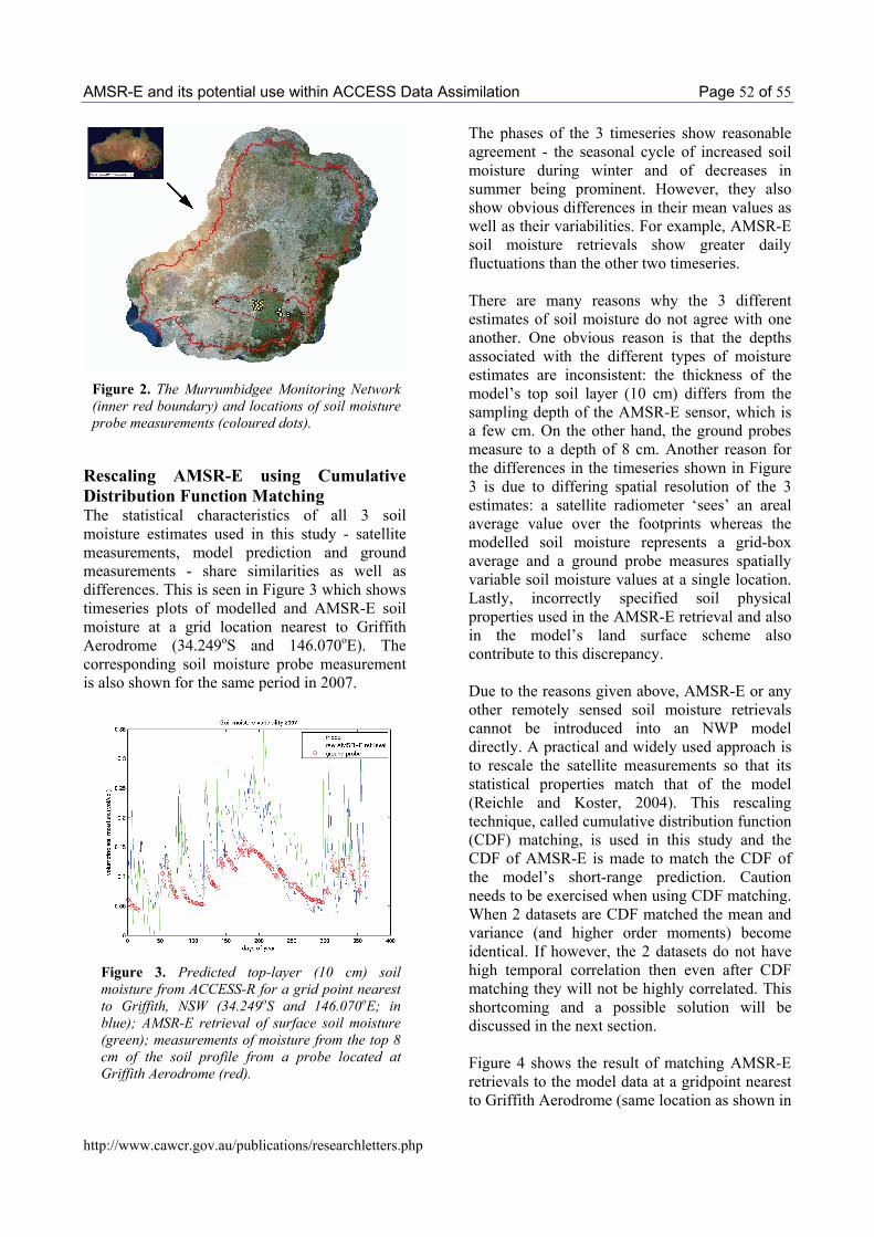
AMSR-E and its potential use within ACCESS Data Assimilation Page 52 of 55
http://www.cawcr.gov.au/publications/researchletters.php
Figure 2. The Murrumbidgee Monitoring Network (inner red boundary) and locations of soil moisture probe measurements (coloured dots).
Rescaling AMSR-E using Cumulative Distribution Function Matching The statistical characteristics of all 3 soil moisture estimates used in this study - satellite measurements, model prediction and ground measurements - share similarities as well as differences. This is seen in Figure 3 which shows timeseries plots of modelled and AMSR-E soil moisture at a grid location nearest to Griffith Aerodrome (34.249oS and 146.070oE). The corresponding soil moisture probe measurement is also shown for the same period in 2007.
Figure 3. Predicted top-layer (10 cm) soil moisture from ACCESS-R for a grid point nearest to Griffith, NSW (34.249oS and 146.070oE; in blue); AMSR-E retrieval of surface soil moisture (green); measurements of moisture from the top 8 cm of the soil profile from a probe located at Griffith Aerodrome (red).
The phases of the 3 timeseries show reasonable agreement - the seasonal cycle of increased soil moisture during winter and of decreases in summer being prominent. However, they also show obvious differences in their mean values as well as their variabilities. For example, AMSR-E soil moisture retrievals show greater daily fluctuations than the other two timeseries. There are many reasons why the 3 different estimates of soil moisture do not agree with one another. One obvious reason is that the depths associated with the different types of moisture estimates are inconsistent: the thickness of the model’s top soil layer (10 cm) differs from the sampling depth of the AMSR-E sensor, which is a few cm. On the other hand, the ground probes measure to a depth of 8 cm. Another reason for the differences in the timeseries shown in Figure 3 is due to differing spatial resolution of the 3 estimates: a satellite radiometer ‘sees’ an areal average value over the footprints whereas the modelled soil moisture represents a grid-box average and a ground probe measures spatially variable soil moisture values at a single location. Lastly, incorrectly specified soil physical properties used in the AMSR-E retrieval and also in the model’s land surface scheme also contribute to this discrepancy. Due to the reasons given above, AMSR-E or any other remotely sensed soil moisture retrievals cannot be introduced into an NWP model directly. A practical and widely used approach is to rescale the satellite measurements so that its statistical properties match that of the model (Reichle and Koster, 2004). This rescaling technique, called cumulative distribution function (CDF) matching, is used in this study and the CDF of AMSR-E is made to match the CDF of the model’s short-range prediction. Caution needs to be exercised when using CDF matching. When 2 datasets are CDF matched the mean and variance (and higher order moments) become identical. If however, the 2 datasets do not have high temporal correlation then even after CDF matching they will not be highly correlated. This shortcoming and a possible solution will be discussed in the next section. Figure 4 shows the result of matching AMSR-E retrievals to the model data at a gridpoint nearest to Griffith Aerodrome (same location as shown in
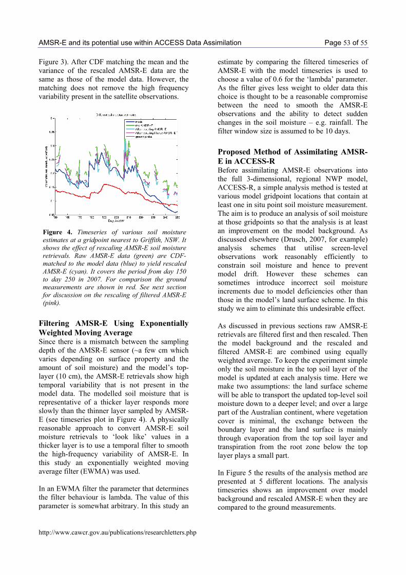
AMSR-E and its potential use within ACCESS Data Assimilation Page 53 of 55
http://www.cawcr.gov.au/publications/researchletters.php
Figure 3). After CDF matching the mean and the variance of the rescaled AMSR-E data are the same as those of the model data. However, the matching does not remove the high frequency variability present in the satellite observations.
Figure 4. Timeseries of various soil moisture estimates at a gridpoint nearest to Griffith, NSW. It shows the effect of rescaling AMSR-E soil moisture retrievals. Raw AMSR-E data (green) are CDF-matched to the model data (blue) to yield rescaled AMSR-E (cyan). It covers the period from day 150 to day 250 in 2007. For comparison the ground measurements are shown in red. See next section for discussion on the rescaling of filtered AMSR-E (pink).
Filtering AMSR-E Using Exponentially Weighted Moving Average Since there is a mismatch between the sampling depth of the AMSR-E sensor (~a few cm which varies depending on surface property and the amount of soil moisture) and the model’s top-layer (10 cm), the AMSR-E retrievals show high temporal variability that is not present in the model data. The modelled soil moisture that is representative of a thicker layer responds more slowly than the thinner layer sampled by AMSR-E (see timeseries plot in Figure 4). A physically reasonable approach to convert AMSR-E soil moisture retrievals to ‘look like’ values in a thicker layer is to use a temporal filter to smooth the high-frequency variability of AMSR-E. In this study an exponentially weighted moving average filter (EWMA) was used. In an EWMA filter the parameter that determines the filter behaviour is lambda. The value of this parameter is somewhat arbitrary. In this study an
estimate by comparing the filtered timeseries of AMSR-E with the model timeseries is used to choose a value of 0.6 for the ‘lambda’ parameter. As the filter gives less weight to older data this choice is thought to be a reasonable compromise between the need to smooth the AMSR-E observations and the ability to detect sudden changes in the soil moisture – e.g. rainfall. The filter window size is assumed to be 10 days.
Proposed Method of Assimilating AMSR-E in ACCESS-R Before assimilating AMSR-E observations into the full 3-dimensional, regional NWP model, ACCESS-R, a simple analysis method is tested at various model gridpoint locations that contain at least one in situ point soil moisture measurement. The aim is to produce an analysis of soil moisture at those gridpoints so that the analysis is at least an improvement on the model background. As discussed elsewhere (Drusch, 2007, for example) analysis schemes that utilise screen-level observations work reasonably efficiently to constrain soil moisture and hence to prevent model drift. However these schemes can sometimes introduce incorrect soil moisture increments due to model deficiencies other than those in the model’s land surface scheme. In this study we aim to eliminate this undesirable effect. As discussed in previous sections raw AMSR-E retrievals are filtered first and then rescaled. Then the model background and the rescaled and filtered AMSR-E are combined using equally weighted average. To keep the experiment simple only the soil moisture in the top soil layer of the model is updated at each analysis time. Here we make two assumptions: the land surface scheme will be able to transport the updated top-level soil moisture down to a deeper level; and over a large part of the Australian continent, where vegetation cover is minimal, the exchange between the boundary layer and the land surface is mainly through evaporation from the top soil layer and transpiration from the root zone below the top layer plays a small part. In Figure 5 the results of the analysis method are presented at 5 different locations. The analysis timeseries shows an improvement over model background and rescaled AMSR-E when they are compared to the ground measurements.
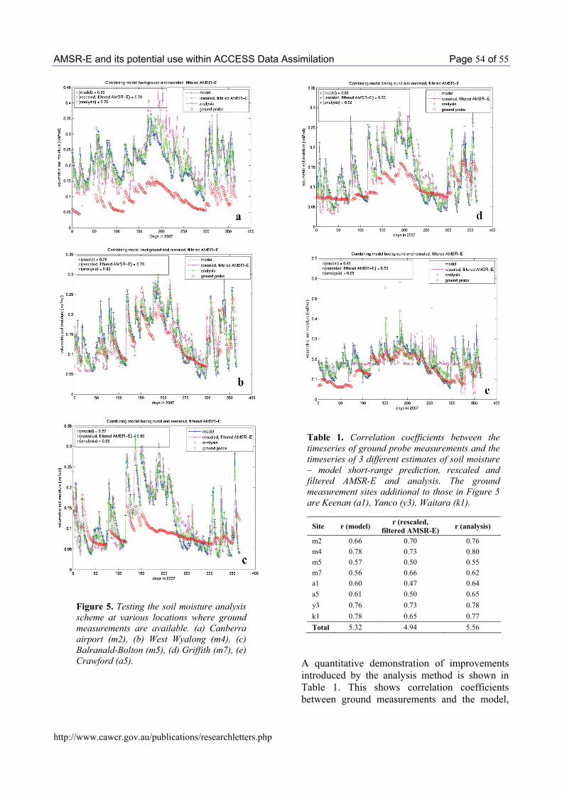
AMSR-E and its potential use within ACCESS Data Assimilation Page 54 of 55
http://www.cawcr.gov.au/publications/researchletters.php
Figure 5. Testing the soil moisture analysis scheme at various locations where ground measurements are available. (a) Canberra airport (m2), (b) West Wyalong (m4), (c) Balranald-Bolton (m5), (d) Griffith (m7), (e) Crawford (a5).
Table 1. Correlation coefficients between the timeseries of ground probe measurements and the timeseries of 3 different estimates of soil moisture – model short-range prediction, rescaled and filtered AMSR-E and analysis. The ground measurement sites additional to those in Figure 5 are Keenan (a1), Yanco (y3), Waitara (k1).
Site r (model) r (rescaled, filtered AMSR-E) r (analysis)
m2 0.66 0.70 0.76 m4 0.78 0.73 0.80 m5 0.57 0.50 0.55 m7 0.56 0.66 0.62 a1 0.60 0.47 0.64 a5 0.61 0.50 0.65 y3 0.76 0.73 0.78 k1 0.78 0.65 0.77 Total 5.32 4.94 5.56
A quantitative demonstration of improvements introduced by the analysis method is shown in Table 1. This shows correlation coefficients between ground measurements and the model,

AMSR-E and its potential use within ACCESS Data Assimilation Page 55 of 55
http://www.cawcr.gov.au/publications/researchletters.php
rescaled and filtered AMSR-E and the analysis respectively. It shows the quality of the analysis improved in a majority of cases.
Summary and Conclusions Inter-comparisons of AMSR-E surface soil moisture retrievals, model short-range forecasts and in situ ground probe measurements show that AMSR-E retrievals contain useful information about near-surface soil moisture. It was shown that cumulative distribution function (CDF) matching rescales the AMSR-E so that it is roughly comparable to the modelled soil moisture. However, it was also shown that this was not enough as the temporal variability in the AMSR-E was high. To overcome this problem an exponentially weighted moving average filter was applied to AMSR-E data before the CDF matching. An analysis was then performed by combining the model background and the rescaled, filtered AMSR-E using equally weighted averaging. The analysis was shown to be a better estimate than the model and in majority of cases the analysis was also better than either the model or the AMSR-E estimate alone, which is what is expected in the case of minimum variance estimation. We expect this assimilation methodology will be an improvement on the current nudging scheme which sometimes introduces erroneous soil moisture increments and the use of AMSR-E is expected to eliminate this undesirable behaviour. We are currently testing the above assimilation method in the ACCESS-R regional system and expect to publish the results in the near future.
Acknowledgements The authors thank Rodger Young of University of Melbourne for providing the Oznet soil moisture data; thank you is extended to Richard de Jeu of Vrije Universiteit Amsterdam for
supplying the AMSR-E retrievals and help in their use. We also thank Adam Smith and Tomasz Glowacki for their thorough review of an earlier draft.
References Betts, A. K. and P. Viterbo, 2005: Land-surface, boundary layer, and cloud-field coupling over the southwestern Amazon in ERA-40, Journal of Geophysical Research, 110, D14108, doi:1029/2004JD005702.
Douville, H., P. Viterbo, J.-F. Mahfouf, and A. Beljaars, 2000: Evaluation of the Optimum Interpolation and Nudging Techniques for Soil Moisture Analysis using FIFE Data, Monthly Weather Review, 128, 1733-1756.
Davies, T., M. J. P. Cullen, A. J. Malcolm, M. H. Mawson, A. Staniforth, A. A. White and N. Wood, 2005: A new dynamical core for the Met Office’s global and regional modelling of the atmosphere, Quarterly Journal of the Royal Meteorological Society, 131, 1759-1782.
Draper, C., J. Walker, P. Steinle, R. de Jeu, and T. Holms, 2009: An evaluation of AMSR-E derived soil moisture over Australia, Remote Sensing and Environment, 113, D03102, doi:10.1016/j.rse.2008.11.011.
Drusch, M., 2007: Initializing numerical weather prediction models with satellite-derived surface soil moisture: Data assimilation experiments with ECMWF’s Integrated Forecast System and the TMI soil moisture data set, Journal of Geophysical Research, 112, D03102, doi:10.1029/2006JD007478.
Entekhabi, D., I. Rodriguez-Iturbe, and F. Castelli, 1996: Mutual interaction of soil moisture state and atmospheric processes, Journal of Hydrology, 184, 3-17.
Owe, M., R. de Jeu, and T. Holmes, 2008: Multisensor historical climatology of satellite-derived global land surface moisture, Journal of Geophysical Research, 113, F01002, doi:10.1029/2007JF000769.
Rawlins, F., S. P. Ballard, K. J. Bovis, A. M. Clayton, D. Li, G. W. Inverarity, A. C. Lorenc and T. J. Payne, 2007: The Met Office global four-dimensional variational data assimilation scheme, Quarterly Journal of the Royal Meteorological Society, 133, 347-362.
Reichle, R., and R. Koster, 2004: Bias reduction in short records of satellite soil moisture, Geophysical Research Letters, 31, L19501, doi:10.1029/2004GL020938.
Reichle, R., and R. Koster, 2005: Global assimilation of satellite surface soil moisture retrievals into the NASA catchment land surface model, Geophysical Research Letters, 32, L02404, doi:10.1029/2004GL02170