ccat science terry herter and ccat science steering committee from codr: 17-jan-06
Post on 22-Dec-2015
221 views
TRANSCRIPT

CCAT Science
Terry Herter and CCAT Science Steering Committee
From CoDR: 17-Jan-06

2
CCAT SSC Membership• Co-Chairs
– Terry Herter (Cornell) and Jonas Zmuidzinas (CIT)• Science Theme Lead
– Distant Galaxies – Andrew Blain (CIT) – Sunyaev-Zeldovich Effect – Sunil Gowala (CIT)– Local galaxies – Gordon Stacey (Cornell)
+ Shardha Jogee (UT)– Galactic Center – Darren Dowell (JPL/CIT)– Cold Cloud Cores Survey – Paul Goldsmith (JPL)
+ Neal Evans (UT)– Interstellar Medium – Jonas Zmuidzinas (CIT)– Circumstellar Disks – Darren Dowell (JPL/CIT)– Kuiper Belt Objects – Jean-Luc Margot (Cornell)
• Ex-officio members– Riccardo Giovanelli (Cornell), Simon Radford (CIT)
3
CCAT Science Strengths• CCAT will be substantially larger and more sensitive than
existing submillimeter telescopes• It will be the first large submillimeter telescope designed
specifically for wide-field imaging• It will complement ALMA
– CCAT will be able to map the sky at a rate hundreds of times faster than ALMA
• CCAT will find galaxies by the tens of thousands • It will map galaxy clusters, Milky Way star-forming
regions, and debris disks
4
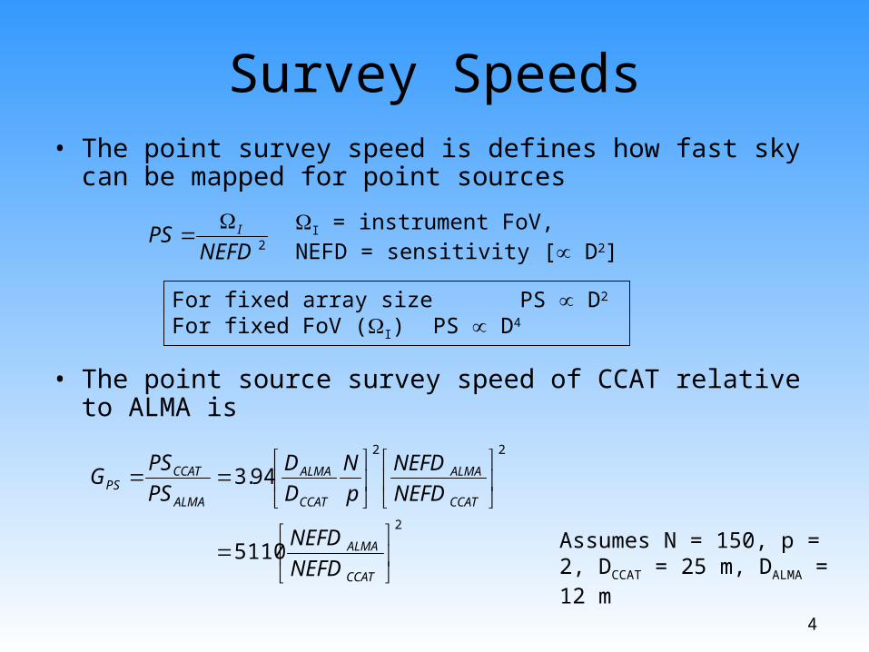
Survey Speeds• The point survey speed is defines how fast sky can be
mapped for point sources
• The point source survey speed of CCAT relative to ALMA is
2
22
5110
94.3
CCAT
ALMA
CCAT
ALMA
CCAT
ALMA
ALMA
CCATPS
NEFD
NEFD
NEFD
NEFD
p
N
D
D
PS
PSG
Assumes N = 150, p = 2, DCCAT = 25 m, DALMA = 12 m
2NEFDPS I
I = instrument FoV, NEFD = sensitivity [ D2]
For fixed array size PS D2 For fixed FoV (I) PS D4
5
Many Sources Peak in the Far-IR/Submillimeter
0.0001
0.001
0.01
0.1
1
10
100
10 100 1000 10000Wavelength (microns)
Flu
x (m
Jy)
Starburst GalaxyKBOCold CoreCCAT Bands
1
2z = 4
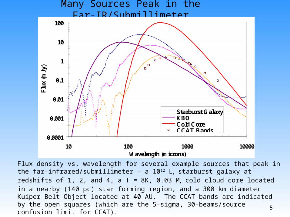
Flux density vs. wavelength for several example sources that peak in the far-infrared/submillimeter – a 1012 L starburst galaxy at redshifts of 1, 2, and 4, a T = 8K, 0.03 M cold cloud core located in a nearby (140 pc) star forming region, and a 300 km diameter Kuiper Belt Object located at 40 AU. The CCAT bands are indicated by the open squares (which are the 5-sigma, 30-beams/source confusion limit for CCAT).

6
Interacting Galaxies
Images of the Antennae (NGC 4038/4039) in the visible (left), infrared (center), and submillimeter (right) showing how the submillimeter reveals regions hidden at shorter wavelengths. For this galaxy and many like it, the submillimeter represents the bulk of the energy output of the galaxy, and reveals the real luminosity production regions which are otherwise hidden. CCAT will have 2.5 times better resolution in the submillimeter giving a spatial resolution like that of the infrared image (center). Credits: visible (HST), infrared (Spitzer), and submillimeter (Dowell et al.)
Visible Infrared Sub-mm
7
Sub-mm is rich in spectral lines
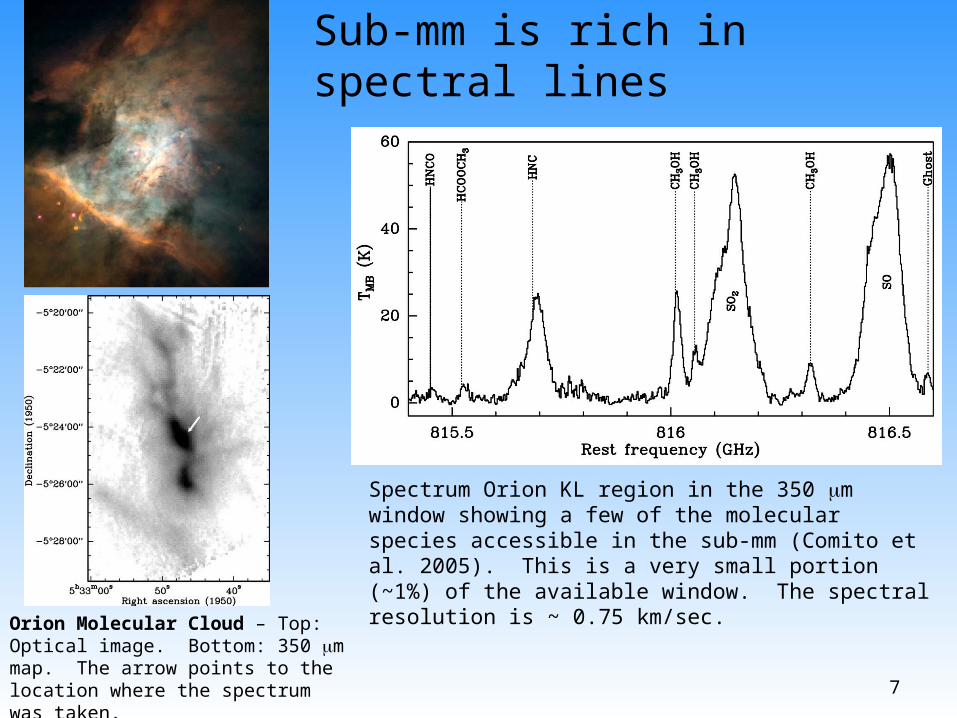
Spectrum Orion KL region in the 350 m window showing a few of the molecular species accessible in the sub-mm (Comito et al. 2005). This is a very small portion (~1%) of the available window. The spectral resolution is ~ 0.75 km/sec.
Orion Molecular Cloud – Top: Optical image. Bottom: 350 m map. The arrow points to the location where the spectrum was taken.
8
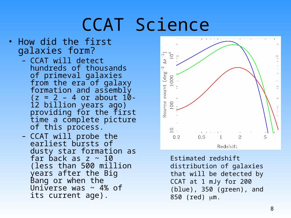
CCAT Science• How did the first galaxies
form?– CCAT will detect hundreds of
thousands of primeval galaxies from the era of galaxy formation and assembly (z = 2 – 4 or about 10-12 billion years ago) providing for the first time a complete picture of this process.
– CCAT will probe the earliest bursts of dusty star formation as far back as z ~ 10 (less than 500 million years after the Big Bang or when the Universe was ~ 4% of its current age).
Estimated redshift distribution of galaxies that will be detected by CCAT at 1 mJy for 200 (blue), 350 (green), and 850 (red) m.

9
Detecting Distant Galaxies
Sensitivity to star formation rate vs. redshift for an Arp 220-like galaxy. All flux limits are set by the confusion limit except for CCAT(200) which is 5 in 104 sec. The conversion used is 2 Msun/yr = 1010 Lsun & LArp220 = 1.3x10¹² Lsun.
Star Formation Sensitivity
1
10
100
1000
0 2 4 6 8 10Redshift
SF
R (
Msu
n/yr
/bea
m)
Spitzer(70) CCAT(200)
CCAT(350) CCAT(450)
CCAT(620) CCAT(740)
CCAT(870) LMT(1100)
Spitzer(24)

10
Large-scale structures
An example of modern cosmological hydrodynamic simulations (Nagamine et al 2005). Each panel has a comoving size of 143 Mpc on a side, and the star forming galaxies with instantaneous star formation rate greater than 100 M/yr at each epoch are indicated by the circles.
1.6 1
2.5
11
CCAT Science – continued• What is the nature of the dark matter and dark energy?
– CCAT will image hundreds of clusters of galaxies selected from current and planned southern-hemisphere cluster searches (via the Sunyaev-Zeldovich Effect).
– CCAT imaging will be important in understanding how clusters form and evolve, and in interpretation and calibration of the survey data to constrain crucial cosmological parameters (M, , dark energy equation of state) independently of other techniques (Type Ia supernova and (direct) CMB measurements).
• How do stars form?– CCAT will survey molecular clouds in our Galaxy to detect the
(cold) cores that collapse to form stars, providing for the first time a complete survey of the star formation process down to very low masses.
– In nearby molecular clouds, CCAT will be able to detect cold cores down to masses well below that of the lowest mass stars (0.08 M).

12
CCAT Science – continued• How do conditions in circumstellar disks determine the
nature of planetary systems and the possibilities for life? – In concert with ALMA, CCAT will study disk evolution from early
(Class I) to late (debris disks) stages.– CCAT will image the dust resulting from the collisional grinding
of planetesimals in planetary systems around other stars allowing determination of the (dynamical) effects of planets on the dust distribution, and hence the properties of the orbits of the planets.
• How did the Solar System form?– The trans-Neptunian region (Kuiper Belt) is a remnant disk that
contains a record of fundamental processes that operated in the early solar system (accretion, migration, and clearing phases).
– CCAT will determine sizes and albedos for hundreds of Kuiper belt objects, thereby providing information to anchor models of the planetary accretion process that occurred in the early solar system.

13
Debris Disks
Image of Fomalhaut debris disk acquired with the CSO/SHARC II (Marsh et al. 2005, ApJ, 620, L47). Left: The observed image which has 10″ resolution and shows a complete ring of debris around the star. Right: A resolution enhanced image with 3″ resolution. CCAT will have this resolution intrinsically, with the capability to achieve ~1″ resolution through image enhancement techniques. From the CSO image, we can already infer the presence of a planet due to the asymmetry of the ring. CCAT imaging should show substructure which will pinpoint the location of the planet. The vertical bars in each image are 40″ in length.
40”
14
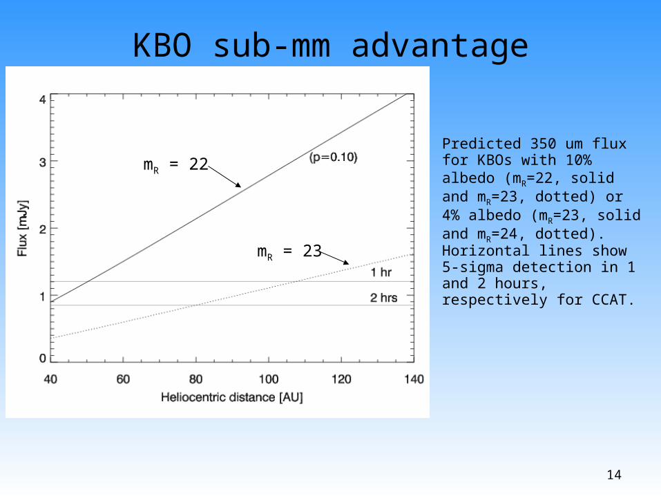
KBO sub-mm advantage
Predicted 350 um flux for KBOs with 10% albedo (mR=22, solid and mR=23, dotted) or 4% albedo (mR=23, solid and mR=24, dotted). Horizontal lines show 5-sigma detection in 1 and 2 hours, respectively for CCAT.
mR = 22
mR = 23
15
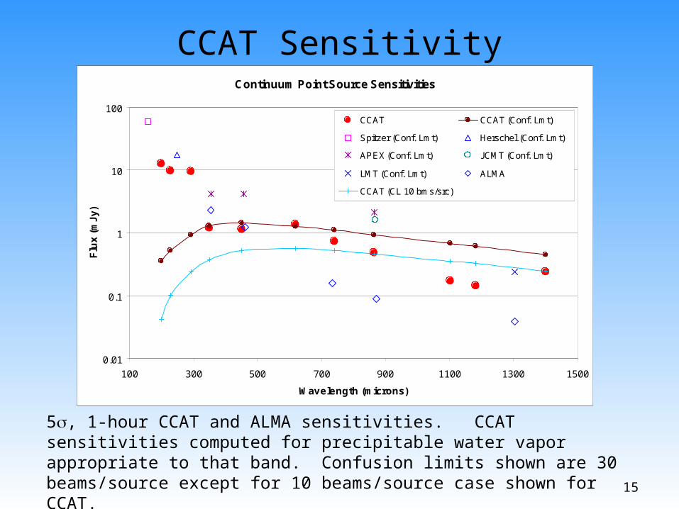
CCAT Sensitivity
5, 1-hour CCAT and ALMA sensitivities. CCAT sensitivities computed for precipitable water vapor appropriate to that band. Confusion limits shown are 30 beams/source except for 10 beams/source case shown for CCAT.
Continuum Point Source Sensitivities
0.01
0.1
1
10
100
100 300 500 700 900 1100 1300 1500
Wavelength (microns)
Flu
x (
mJ
y)
CCAT CCAT (Conf. Lmt)
Spitzer (Conf. Lmt) Herschel (Conf. Lmt)
APEX (Conf. Lmt) JCMT (Conf. Lmt)
LMT (Conf. Lmt) ALMA
CCAT (CL 10 bms/src)
5.0-sigma in 3600 sec
16
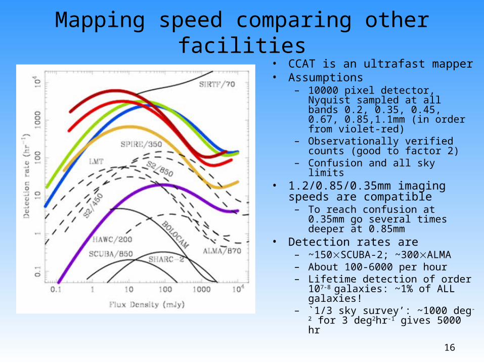
Mapping speed comparing other facilities• CCAT is an ultrafast mapper• Assumptions
– 10000 pixel detector, Nyquist sampled at all bands 0.2, 0.35, 0.45, 0.67, 0.85,1.1mm (in order from violet-red)
– Observationally verified counts (good to factor 2)
– Confusion and all sky limits• 1.2/0.85/0.35mm imaging speeds
are compatible– To reach confusion at 0.35mm go
several times deeper at 0.85mm• Detection rates are
– ~150SCUBA-2; ~300ALMA– About 100-6000 per hour– Lifetime detection of order 107-8
galaxies: ~1% of ALL galaxies! – `1/3 sky survey’: ~1000 deg-2 for 3
deg2hr-1 gives 5000 hr
17
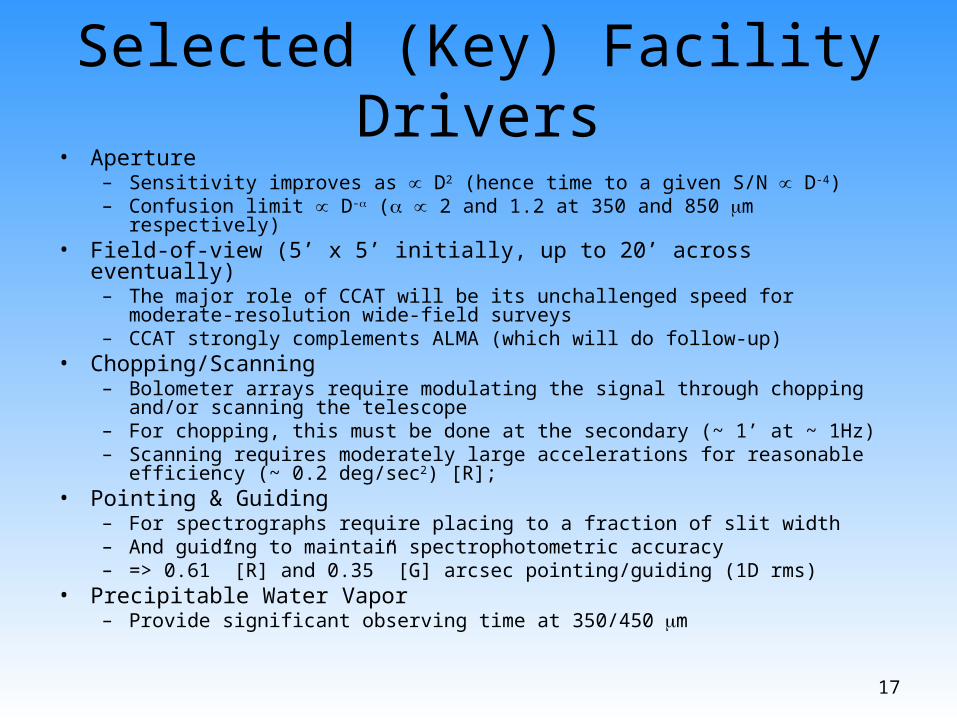
Selected (Key) Facility Drivers• Aperture
– Sensitivity improves as D2 (hence time to a given S/N D-4)– Confusion limit D- ( 2 and 1.2 at 350 and 850 m respectively)
• Field-of-view (5’ x 5’ initially, up to 20’ across eventually)– The major role of CCAT will be its unchallenged speed for moderate-resolution
wide-field surveys– CCAT strongly complements ALMA (which will do follow-up)
• Chopping/Scanning– Bolometer arrays require modulating the signal through chopping and/or
scanning the telescope– For chopping, this must be done at the secondary (~ 1’ at ~ 1Hz)– Scanning requires moderately large accelerations for reasonable efficiency (~ 0.2
deg/sec2) [R]; • Pointing & Guiding
– For spectrographs require placing to a fraction of slit width– And guiding to maintain spectrophotometric accuracy– => 0.61” [R] and 0.35” [G] arcsec pointing/guiding (1D rms)
• Precipitable Water Vapor– Provide significant observing time at 350/450 m
18
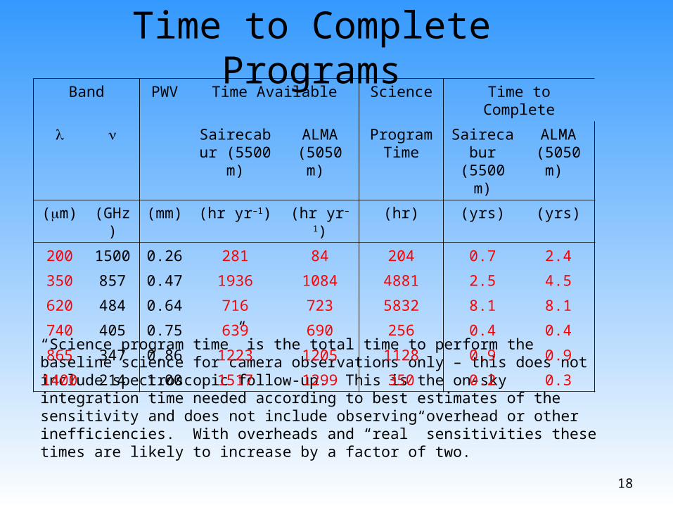
Time to Complete Programs
“Science program time” is the total time to perform the baseline science for camera observations only – this does not include spectroscopic follow-up. This is the on-sky integration time needed according to best estimates of the sensitivity and does not include observing overhead or other inefficiencies. With overheads and “real” sensitivities these times are likely to increase by a factor of two.
Band PWV Time Available Science Time to Complete
Sairecabur (5500 m)
ALMA (5050 m)
Program Time
Sairecabur (5500 m)
ALMA (5050 m)
(m) (GHz) (mm) (hr yr–1) (hr yr–1) (hr) (yrs) (yrs)
200 1500 0.26 281 84 204 0.7 2.4
350 857 0.47 1936 1084 4881 2.5 4.5
620 484 0.64 716 723 5832 8.1 8.1
740 405 0.75 639 690 256 0.4 0.4
865 347 0.86 1223 1205 1128 0.9 0.9
1400 214 1.00 1517 1299 350 0.2 0.3

19
Next Phase• Refinements
– What have we left out?– Parametric trade analysis, e.g. when surface roughness changes, how
do program times change.• Detailed survey planning
– Teaming – bring together necessary expertise– Selection of fields and/or objects– Institute critical precursor surveys (e.g. Spitzer) or other observations
• Data reduction requirements– Establish requirements:
• Quicklook tools, pipelines, etc.• Calibration
• Data analysis– Identifying steps to produce science from calibrated data
• Archiving– Scope out problem in more detail – storage, access requirements,
processing/reduction level, etc.

20
End of Presentation
• Spare slides follow

21
CCAT Science Steering Committee Charter
• Establish top-level science requirements– Determine and document major science themes
• Flow down science requirements to facility requirements– Telescope, instrumentation, site selection criteria, operations,
etc.
• Outputs– Science document
• Write-ups on major science themes using uniform format (science goals, motivation/background, techniques, CCAT requirements, uniqueness and synergies)
– Requirements document• Specifies requirements for aperture, image quality, pointing,
tracking, scanning, chopping, etc.
22
Submm Number Counts
1
10
100
1000
10000
100000
1000000
10000000
0.001 0.01 0.1 1 10 100 1000
S (mJy)
Nu
mb
er
> S
/ sq
. de
g
200 um 350 um
450 um 620 um
740 um 865 um
1100 um 1400 um
2000 um 3300 um
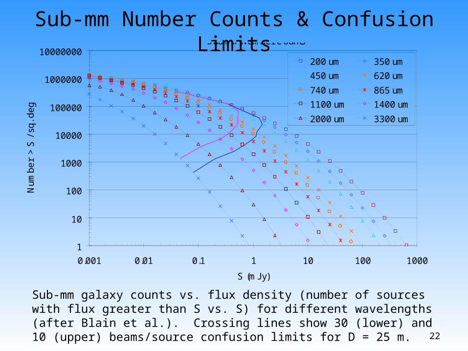
Sub-mm Number Counts & Confusion Limits
Sub-mm galaxy counts vs. flux density (number of sources with flux greater than S vs. S) for different wavelengths (after Blain et al.). Crossing lines show 30 (lower) and 10 (upper) beams/source confusion limits for D = 25 m.
23
Time Available to Observe
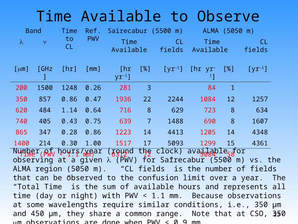
Number of hours/year (round the clock) available for observing at a given (PWV) for Sairecabur (5500 m) vs. the ALMA region (5050 m). “CL fields” is the number of fields that can be observed to the confusion limit over a year. The “Total Time” is the sum of available hours and represents all time (day or night) with PWV < 1.1 mm. Because observations at some wavelengths require similar conditions, i.e., 350 µm and 450 µm, they share a common range. Note that at CSO, 350 m observations are done when PWV < 0.9 mm.
Band Time to CL
Ref.PWV
Sairecabur (5500 m) ALMA (5050 m)
Time Available CL fields Time Available CL fields
[m] [GHz] [hr] [mm] [hr yr–1] [%] [yr–1] [hr yr–1] [%] [yr–1]
200 1500 1248 0.26 281 3 84 1
350 857 0.86 0.47 1936 22 2244 1084 12 1257
620 484 1.14 0.64 716 8 629 723 8 634
740 405 0.43 0.75 639 7 1488 690 8 1607
865 347 0.28 0.86 1223 14 4413 1205 14 4348
1400 214 0.30 1.00 1517 17 5093 1299 15 4361
Time (PWV < 1.1 mm) 6312 72 5084 58
24
Time to Complete Programs
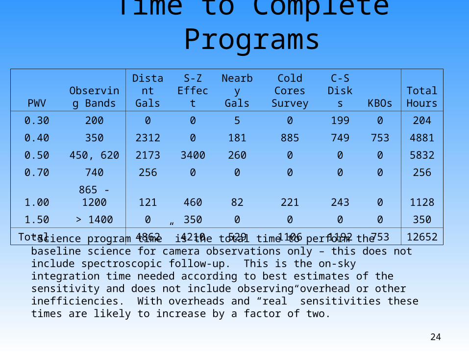
“Science program time” is the total time to perform the baseline science for camera observations only – this does not include spectroscopic follow-up. This is the on-sky integration time needed according to best estimates of the sensitivity and does not include observing overhead or other inefficiencies. With overheads and “real” sensitivities these times are likely to increase by a factor of two.
PWVObserving
BandsDistant Gals
S-Z Effect
Nearby Gals
Cold Cores Survey
C-S Disks KBOs
Total Hours
0.30 200 0 0 5 0 199 0 204
0.40 350 2312 0 181 885 749 753 4881
0.50 450, 620 2173 3400 260 0 0 0 5832
0.70 740 256 0 0 0 0 0 256
1.00865 - 1200 121 460 82 221 243 0 1128
1.50 > 1400 0 350 0 0 0 0 350
Total 4862 4210 529 1106 1192 7531265
2

25
0.1
1
10
100
1000
10000
100000
0 500 1000 1500 2000 2500
Wavelength (microns)
Sp
ee
d (
sq-'/
hr/
mJy
^2)
CCAT APEX
Scuba-2 CSO
LMT Herschel
Mapping Speed
Rate at which sky can be mapped (array/NEFD2). This is a measure of how quickly sky can be covered to a give flux level providing the confusion limit is not reached. Calculation assumes 150x150 array with 2 pixels/res. element with max 20' FoV for CCAT, APEX & CSO. FoV is 8' FoV for JCMT & LMT and 4' FoV for Herschel.
26
Confusion Limits w/ Galaxies/hr to C.L.
-1
0
1
2
3
4
5
6
0 500 1000 1500 2000 2500
Wavelength (microns)
5-s
igm
an
C.L
. (m
Jy)
CSO APEX
CCAT Scuba-2
LMT
Confusion Limits
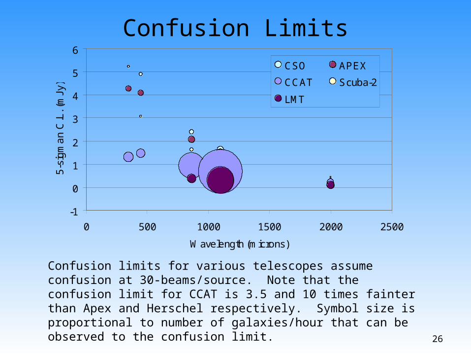
Confusion limits for various telescopes assume confusion at 30-beams/source. Note that the confusion limit for CCAT is 3.5 and 10 times fainter than Apex and Herschel respectively. Symbol size is proportional to number of galaxies/hour that can be observed to the confusion limit.
27
1
10
100
1000
10000
0 500 1000 1500 2000 2500
Wavelength (microns)
Ga
laxi
es/
hr
to C
.L.
CSO APEX
CCAT Scuba-2
LMT
Galaxy Detection Rate at Confusion Limit
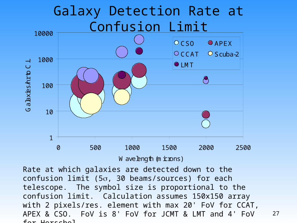
Rate at which galaxies are detected down to the confusion limit (5, 30 beams/sources) for each telescope. The symbol size is proportional to the confusion limit. Calculation assumes 150x150 array with 2 pixels/res. element with max 20' FoV for CCAT, APEX & CSO. FoV is 8' FoV for JCMT & LMT and 4' FoV for Herschel.

28
Facility
Lambda(micron
s)Freq.(GHz)
Beam Diam.
(arcsec)
Array FoV
(arcmin)
f
(mJy)
Conf. Limit(mJy)
Time to
Conf. Limit(sec)
Conf. Limit src density(#/sq-deg)
Survey Speed
(arcmin/ hr/
mJy^2)
Gals/hr to CL
Gals on Array
f >= CL
Gals on Arrayf >= f
CCAT 350 857 3.81 4.76 1.25 1.29 3384 37856 14 251 236 243
450 667 4.90 4.75 1.18 1.45 2392 22901 16 213 142 180
865 347 9.42 19.6 0.57 0.92 1357 6198 1202 1772 668 1384
1100 273 11.2 20.0 0.19 0.67 290 3833 11030 5325 429 2950
2000 150 21.8 19.6 0.20 0.20 3730 1159 9684 134 139 134
APEX 350 857 7.94 9.93 7.03 4.27 9767 8722 2.0 89 242 117
450 667 10.2 12.8 6.25 4.09 8413 5276 4.2 106 249 127
865 347 19.6 19.8 2.27 2.06 4375 1428 76 144 175 146
1100 273 25.0 19.8 0.78 1.41 1100 883 647 354 108 325
2000 150 45.4 19.9 0.85 0.39 17217 267 549 7.1 34.2 5.2
JCMT 450 667 8.17 7.94 8.55 3.05 28325 8244 0.9 19 149 27
865 347 15.7 7.96 1.83 1.63 4578 2231 19 34 43 35
1100 273 20.0 7.99 0.61 1.13 1060 1380 169 91 27 80
2000 150 36.3 7.87 0.61 0.32 13349 417 166 2.2 8.3 1.8
CSO 350 857 9.16 11.5 19.0 5.21 47733 6551 0.4 18 243 29
450 667 11.8 14.7 12.8 4.90 24705 3963 1.3 36 250 47
865 347 22.6 20.0 3.73 2.39 8768 1073 29 56 135 57
1100 273 28.8 19.9 1.24 1.62 2111 663 258 148 83 140
2000 150 52.4 19.6 1.26 0.44 29283 201 243 3.1 25 1.8
LMT 865 347 4.71 8.01 0.49 0.38 6173 24791 266 235 403 282
1100 273 5.99 7.99 0.11 0.30 465 15330 5482 1914 247 974
2000 150 10.9 7.99 .065 .096 1651 4637 15072 181 83 155
Herschel 200 1500 15.6 3.89 1.42 15.9 29 2272 7.5 1212 9.6 174
350 857 27.2 4.08 1.50 19.6 21 742 7.4 588 3.5 148
450 667 35.0 4.08 1.71 17.1 36 449 5.7 206 2.1 86Flux density is 5 in 1 hour, confusion limits (CL) are 30 beams/source, and time to CL is for 5 at CL.
CCAT vs. Other Facilities