cchheemmiiccaall rreeaaccttiioonn rraattee … · · 2009-12-03background – chemistry 6...
TRANSCRIPT

CO3120 Final Report submitted to the University of Leicester in Partial Fulfilment for the
degree of Bachelor of Science
.
CChheemmiiccaall RReeaaccttiioonn RRaattee AAnnaallyyssiiss
UUssiinngg GGrraapphh TTrraannssffoorrmmaattiioonnss
CO3120 Computer Science Project
Final Report
May 2009
Mayur Bapodra

Mayur Bapodra i CO3120 Final Report
Contents
Contents i
Tables and Figures iii
Declaration 1
Abstract 2
1. Introduction 3 Motivation 3 Aims 4 Objectives 4 Outcomes 5
2. Background – Chemistry 6 Literature survey 6 The rate constant, k 7 A simple one-step reaction 9 More complex reaction mechanisms 10 Use of a stoichiometric matrix 11
3. Background – Graph Transformations 13 Literature survey 13 Graphs and type graphs 16 Graph transformations 18 Critical pairs 19 Stochastic graph transformations & reaction networks 21
4. Molecular Representation Using Graphs 24 1st attempt 24 2nd attempt 26 3rd attempt 28
5. Methodology 31 Use of critical pairs 31 Step 1: Specification of reaction rules and starting materials in AGG 32 Step 2: Application of reaction rules to the start graph to obtain intermediates 32 Step 3: Execution of first pass critical analysis 33 Step 4: Removal of structurally equivalent overlappings 33 Step 5: Manual observation of results and instantiation of rules 34 Step 6: Disabling of original general rules, and renaming of all rules 35 Step 7: Execution of critical pair analysis with fully instantiated rules 35 Step 8: Removal of structurally equivalent overlappings for instantiated rules 36 Step 9: Execution of ODE extraction program 37 Step 10: Solving ODE’s using a 3rd party math solver 37
6. Implementation 39 Tools that implement the methodology 39 The AGG API 42 Critical Pair Analysis 43 Structural Equivalence Testing 45 ODE Extraction 46

Mayur Bapodra ii CO3120 Final Report
Running the Kinetic Analysis 47
7. Case Study 1 – Esterification 50 Step 1 50 Step 2 53 Step 3 53
8. Case Study 2 – SN1 Reaction 54 Step 1 54 Step 2 58 Step 3 59 Step 4 61 Step 5 61 Step 6 63 Step 7 63 Step 8 64 Step 9 65 Brief Analysis of results 66
9. Planning and Timescales 67 Tasks 67 Challenges and Rsks 70 Deliverables 71 Gantt Chart 71 Appraisal of Plan 73
10. Critical Appraisal 75 Summary of completed work 75 Self-assessment 75 Suggestions for further work 77
Bibliography 79
Appendix 1 – Career Plan 81
Appendix 2 – Weekly Diaries 83
Mayur Bapodra iii CO3120 Final Report
Tables and Figures
Figure 1 – energy profile depiction of activation energy 8
Figure 2 - simple SN2 reaction (hydrolysis of ethyl chloride to ethanol) 9
Figure 3 - example of complex reaction mechanism 10
Figure 4 – stoichiometric matrix for example reaction 11
Figure 5 - rate law matrix for example reaction 12
Figure 6 - example type graph 17
Figure 7 - example typed graph 17
Figure 8 - definition of a graph transformation (DPO) 18
Figure 9 - definition of graph transformation with match 18
Figure 10 - example rule 1 18
Figure 11 - rule 1 applied to example graph in figure 7 19
Figure 12 - parallel independence of rules [4] 19
Figure 13 - double pushout depiction of parallel independence [9] 20
Figure 14 - double pushout depiction of sequential independence [9] 20
Figure 15 - example Q-matrix 22
Figure 16 - esterification type graph, 1st attempt 24
Figure 17 - esterification start graph, 1st attempt 25
Figure 18 - atomic constraint for 1st attempt type graph 26
Figure 19 - hyperedge representation of CH4 27
Figure 20 - bipartite graph representation of CH4 27
Figure 21 - esterification type graph, 2nd attempt 28
Figure 22 - esterification start graph, 2nd attempt 28
Figure 23 - esterification type graph, final version 29
Figure 24 - esterification start graph, final version 29
Figure 25 - example bond node constraint for final type graph 30
Figure 26 - structural representation of ethanoic acid 32
Figure 27 - example of chemically equivalent structural overlappings 34
Figure 28 - double pushout construction depicting instantiation of rule 35
Figure 29 - AGG critical pair conflicts summary example 36
Figure 30 - AGG critical pair conflicts summary example after structural equivalence reduction 37
Figure 31 - main layout of AGG 39
Figure 32 - kinetic analysis program, steps 2 and 3 40
Figure 33 - critical pair analysis GUI module of AGG 41
Figure 34 - result of running complete kinetic analysis suite 42
Figure 35 - critical pair analysis package structure 43

Mayur Bapodra iv CO3120 Final Report
Figure 36 - step 1 of esterification reaction [3] 50
Figure 37 - step 1 of esterification reaction, GT rule 50
Figure 38 - step 2 of esterification reaction [3] 51
Figure 39 - step 2 of esterification reaction, GT rule 51
Figure 40 - step 3 of esterification reaction [3] 51
Figure 41 - step 3 of esterification reaction, GT rule 51
Figure 42 - step 4 of esterification reaction [3] 52
Figure 43 - step 4 of esterification reaction, GT rule 52
Figure 44 - step 5 of esterification reaction [3] 52
Figure 45 - SN1 type graph 54
Figure 46 - constraint limiting number of bonds allowed 55
Figure 47 - constraint designating direction of edges in bonds 55
Figure 48 - constraint limiting C and C+ connection to same bond node 55
Figure 49 - SN1 starting materials 56
Figure 50 - step 1 of SN1 reaction 56
Figure 51 - step 1 of SN1 reaction, GT rule 56
Figure 52 - step 2 of SN1 reaction 57
Figure 53 - step 2 of SN1 reaction, GT rule 57
Figure 54 - step 3 of SN1 reaction 57
Figure 55 - step 3 of SN1 reaction, GT rule 57
Figure 56 - reaction of CH3OH with CH3+ 62
Figure 57 - instantiation of step2 for reaction with water 62
Figure 58 - instantiation of step2 for reaction with methanol 62
Figure 59 - NAC for step2 general rule to create instantiated rule 63
Table 1 - delete-use overlapping information for esterification - conflicts 53
Table 2 - preliminary intermediates in SN1 reaction 59
Table 3 - summary of conflict overlappings from critical pair analysis (first pass) 60
Table 4 - summary of dependency overlappings from critical pair analysis (first pass) 60
Table 5 - delete-use overlapping information for SN1 - conflicts 61
Table 6 - delete-use overlapping information for SN1 - dependencies 61
Table 7 - summary of conflict overlappings from critical pair analysis (final pass) 64
Table 8 - summary of dependency overlappings from critical pair analysis (final pass) 64
Table 9 - summary of conflict overlappings after structural equivalence analysis 65
Table 10 - - summary of dependency overlappings after structural equivalence analysis 65
Code 1 - CPAnalysisSetup, setUpRules method 43
Code 2 - MB294ExcludePairContainer, fillContainers method 44

Mayur Bapodra v CO3120 Final Report
Code 3 - MB294DependencyPairContainer, computeCritical method 44
Code 4 - MB294ComputeCriticalPairs, use of MB294ParserFactory 45
Code 5 - structural equivalence testing package structure 45
Code 6 - ODE extraction package structure 46
Code 7 - ODEExtraction, outputODEs method 47
Code 8 - StructuralEquivalenceAnalysis, main method demonstrating use of exit codes 48
Code 9 - MB294CriticalPairAnalysis, main method 48
Code 10 - Windows batch script demonstrating use of Java system exit codes 49

Mayur Bapodra 1 CO3120 Final Report
Declaration
All sentences or passages quoted in this report, or computer code of any form whatsoever
used and/or submitted at any stages, which are taken from other people‟s work have been
specifically acknowledged by clear citation of the source, specifying author, work, date and
page(s).
Any part of my own written work, or software coding, which is substantially based upon
other people‟s work, is duly accompanied by clear citation of the source, specifying author,
work, date and page(s).
I understand that failure to do this amounts to plagiarism and will be considered grounds for
failure in this module and the degree examination as a whole.
Name: Mayur Bapodra
Signed:
Date:

Mayur Bapodra 2 CO3120 Final Report
Abstract
The following report documents the outcome of a yearlong project aimed at the derivation of
ordinary differential equations for a chemical reaction, using graph transformation techniques.
While some articles have described the application of graph transformation techniques to
biochemical reactions, and the use of stochastic systems to predict the kinetic profiles of
reactions, very few have tried to derive these linear differential equations.
The report first describes the original motivation, aims and objectives for the project. Then, a
background in chemistry is included, which describes the manual derivation of ordinary
differential equations for a reaction. A summary of relevant graph transformation theory used
in the project is also presented. The report briefly describes here some of the research done
last term into stochastic graph transformation systems, which provide a foundation to the
method eventually developed.
The project core follows, which describes in detail, our developed methodology used to
generate the ordinary differential equations for a specific finite reaction network, the
adaptation of existing tools that facilitates the application of this methodology, and two case
studies to demonstrate this application.
In the final section of the report, there is a discussion of how functional and useful the
original project plan was, finding many difficulties in the precise projection of timescales for
an open-ended problem such as this. Finally, a critical appraisal focuses on the limitations of
the project, such as the limited applicability of the developed methodology, problems with
the software used and many suggestions for areas of further work. The project has successful
results for one simple reaction (unimolecular nucleophilic substitution, SN1) with very small
starting molecules, but limitations in 3rd
party analysis tools rendered it useless for testing
larger reaction networks and larger molecules. Further work is necessary to investigate how
to make analysis faster and more efficient if it is to be of any widespread use for chemists.
Nevertheless, the successful case study demonstrates the soundness of the methodology in
principle.

Mayur Bapodra 3 CO3120 Final Report
1. Introduction
Motivation
The kinetics of any chemical reaction is important for many areas of research, whether it is
deducing the reactivity of certain reagents in the lab, or for planning large scale industrial
chemical synthesis. The speed at which reactions occur is vital knowledge for any such
undertaking. Traditionally, chemists are able to conduct experiments in the lab that ascertain
this information. The findings of such experiments relate to the observer important facets of
the underlying reaction, such as the stabilities of any chemical species involved or the steps
that might have occurred from the starting molecule to the product molecule. This process
can however be reversed – by proposing a reaction mechanism and comparing it to
experimental data, chemists can gauge the accuracy of their proposals. This offers a way of
gaining a deeper understanding of the elemental chemistry behind any complex reaction.
This project aims to derive the ordinary differential equations that describe the kinetics of any
reaction using graph transformation techniques. While these equations can be derived by
hand, it becomes extremely difficult for unbounded and complex reaction networks.
Automation of this process would make it more widely applicable and therefore more useful.
Related work in this field has mainly focused on stochastic graph transformation simulations
to produce quantitative data rather than the derivation of these linear algebraic equations. The
results of such simulations are affected by hardware capabilities (specifically in the number
of starting molecules allowed in the system). Ordinary differential equations however, are an
alternative level of abstraction with a reproducible result. This result should be utilisable
under different conditions to predict the progress of a reaction, whereas the simulation results
are specific to the conditions and probabilistic circumstances under which it was run. The two
approaches should be used together however to determine their congruence and therefore the
accuracy of the proposed reaction mechanism.
While others, such as Cardelli [2], have derived these ordinary differential equations using
alternative methods ([2] uses process algebra), these are not intuitive for chemists to use due
to their technical content. Graph transformations remain relatively unexplored in this area,
despite their visual attractiveness and simplicity. Chemists already used to using graphs (i.e.
structural formula) to represent molecules would be more comfortable with an approach that
bears some resemblance to this application domain. If a computer science method of deriving
ordinary differential equations were to be widely applicable, graph transformation systems
seem to be the most promising. Furthermore, Cardelli‟s process calculus approach requires
the establishment of reaction rules that describe involved reactants in their entirety. Graph
transformations allow the specification of rules based on functional groups i.e. only the atoms
and bonds directly affected by a reaction. This more general specification makes reaction
rules reusable in many molecules based on local context.
This task is not trivial, however. The first obstacle is a representation of molecules and
reactions in graphs that retains as much of the real chemistry as possible while not
complicating the computational analysis. The eventual balance requires an understanding of
both the underlying chemistry and the computer science theory. Secondly, the derivation of
ordinary differential equations by hand is a complex procedure that could require a number of
sequential or repetitive steps. Such a procedure may not only be unappealing to computer
scientists to replicate, but also difficult to do so in an uncomplicated way. This project aims
to take the first steps towards such a methodology. This methodology once evolved and
Mayur Bapodra 4 CO3120 Final Report
improved upon further will aid the automated derivation of ordinary differential equations for
simple finite systems, and more importantly, for open infinite reaction mechanisms too, such
as polymerisation.
Aims
The project aims to develop a methodology to analyse the quantitative dynamics of chemical
reactions, namely in determining the ordinary differential equations (ODE‟s) which define
the rate of reaction. This rate is usually determined as the rate of change of concentration of
one of the chemical species (which can be reactants or products) with respect to time. These
differential equations will be extracted from a specification of reaction rules as local
structural transformations in molecules represented as graphs. The methodology will be
verified against actual case studies using appropriate tools.
Objectives
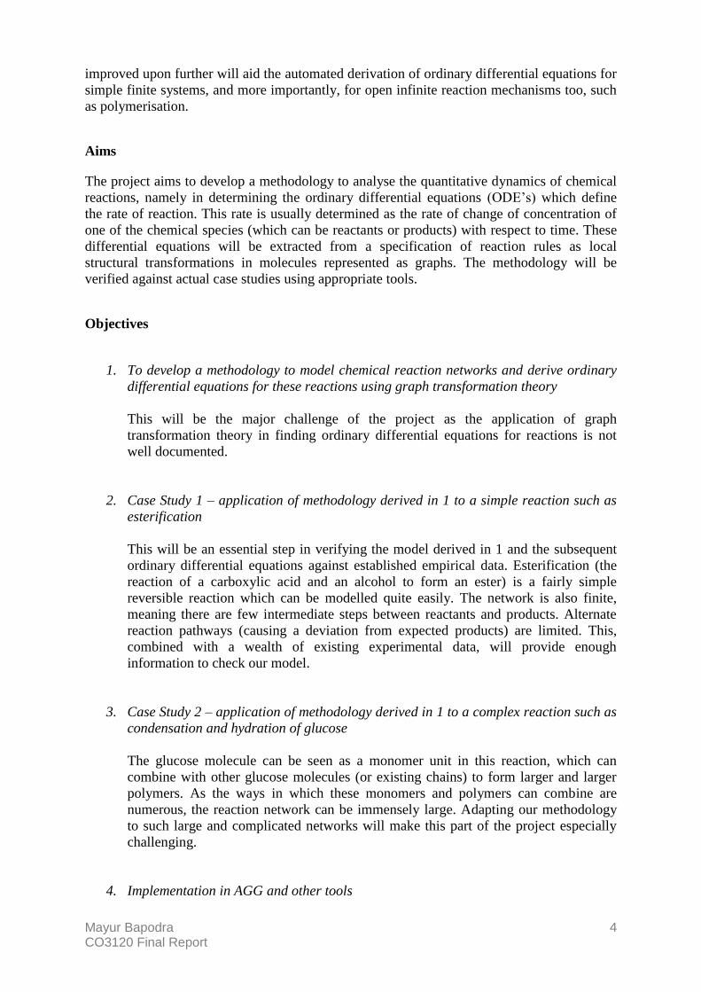
1. To develop a methodology to model chemical reaction networks and derive ordinary
differential equations for these reactions using graph transformation theory
This will be the major challenge of the project as the application of graph
transformation theory in finding ordinary differential equations for reactions is not
well documented.
2. Case Study 1 – application of methodology derived in 1 to a simple reaction such as
esterification
This will be an essential step in verifying the model derived in 1 and the subsequent
ordinary differential equations against established empirical data. Esterification (the
reaction of a carboxylic acid and an alcohol to form an ester) is a fairly simple
reversible reaction which can be modelled quite easily. The network is also finite,
meaning there are few intermediate steps between reactants and products. Alternate
reaction pathways (causing a deviation from expected products) are limited. This,
combined with a wealth of existing experimental data, will provide enough
information to check our model.
3. Case Study 2 – application of methodology derived in 1 to a complex reaction such as
condensation and hydration of glucose
The glucose molecule can be seen as a monomer unit in this reaction, which can
combine with other glucose molecules (or existing chains) to form larger and larger
polymers. As the ways in which these monomers and polymers can combine are
numerous, the reaction network can be immensely large. Adapting our methodology
to such large and complicated networks will make this part of the project especially
challenging.
4. Implementation in AGG and other tools

Mayur Bapodra 5 CO3120 Final Report
The graph transformation rules and an initial graph representing the reactant
molecules can be implemented in AGG [19]. AGG is a programming tool commonly
used by the graph transformation community as it has a natural, user-friendly
interface. AGG can apply constructed rules to input graphs in order to test whether
they produce the proper results, which is a fundamental step towards deriving ODE‟s.
Some additional work using the AGG API will be necessary to adapt the software to
our needs, and to automate certain steps in our analysis.
There is also a secondary personal learning objective outlined below:
5. To gain a thorough understanding of graph transformation theory
As well as revising the background knowledge from the fields of Chemistry and
Physics needed for the project, research into graph transformation theory will be
necessary. This will include basic theory, stochastic theory, and also ways in which
graph transformation theory can be applied to chemical reaction networks.
The aims and objectives of the project have changed somewhat since the initial inception
phase (see original project description form) as understanding of the problem has become
clearer through extensive reading and consultation with supervisors. In particular, the
following modifications have been made:
Universal rules governing the general reactivity of functional groups as influenced by
intramolecular factors and the availability of other reacting species will not be
implemented. This in itself is a large task that bears little relation to the more
specialized main aim of defining reaction kinetics. Furthermore, such reaction
predicting systems have already been successfully implemented by others. Therefore,
only the rules directly affecting the case studies will be investigated and implemented.
The development of an interface specifically designed for chemists constructing graph
transformation systems has been abandoned as this has also been accomplished by
others. In addition, development of such a system would be independent of the other
major objectives of the project. In order to plan a more coherent and self-contained
project, and to leave time for other more important parts of the project, existing tools
(such as AGG) will be used without adapting them to a chemistry-related paradigm.
Outcomes
The project produced a methodology to derive ordinary differential equations for multistep
reaction mechanisms. An implementation of the methodology was also developed to test its
practicality. This was verified against a simple case study of the SN1 reaction. The
methodology has some deficiencies and limits to its universal applicability as discussed in the
critical appraisal. Specifically, it currently focuses on reaction networks with a finite number
of rules. Due to scalability limitations in the 3rd
party tools used, the implementation only
works for reaction mechanisms involving molecules of bounded size and with reaction rules
where local context in the left hand side of the rule is limited to a few atoms and bonds.
Nevertheless the project is a useful and successful first step towards achieving our aims.

Mayur Bapodra 6 CO3120 Final Report
2. Background – Chemistry
This chapter outlines first the literature survey conducted as part of the “Project Plan” and
provides an overview of the main ideas from Chemistry pertaining to the project. A more
detailed treatment then follows explaining methodically how ordinary differential equations
for a reaction can be extracted from its mechanism.
Literature survey
Before the analysis of kinetics can take place for chemical reactions, an understanding of how
molecules react must be gained. Any basic course or text book in Organic Chemistry is useful
here but [13] provides a thorough university-level description of reaction kinetics. In
particular, it is useful because it derives formulas commonly associated with kinetics from
first principles. An appreciation of this may prove fundamental when developing our model
of reaction networks and especially when deriving differential equations.
In the simplest terms, chemical reactions occur when the bonds in molecules break and/or
form. Some reactions are fairly simple and involve only one or very few steps. The rate laws
for these reactions can be predicted fairly easily. Others however involve numerous steps,
each step known as an elementary step in the overall reaction mechanism. Predicting,
deriving or interpreting experimental data for such reactions can be complicated and may
involve approximations and assumptions which reduce the validity of results. The mechanism
is also not entirely deterministic. At any step, there may be several choices for subsequent
steps. These steps may not be equally likely but probable nonetheless and could lead to by-
products.
Reaction between two molecules can be prompted by collision with each other where the
collision is energetic enough to cause the breaking of a bond and the formation of another
bond. The minimum energy needed for reaction (provided by the collision) is denoted by the
Activation Energy (this is an important concept as this energy is directly related to the rates
of elementary reactions). The activation energy is greater than or equal to the difference in
the stable energies of the reactants and products. In reactions where the reactants are
particularly stable compared to the products, collision between the reactant molecules is often
the determining factor of whether a reaction can take place or not. The collision step is
known as the rate determining step in this case. Reactions do not always occur through
collision however. If a molecule has an extremely reactive leaving group (a group in a
molecule which can accept electrons from a carbon and break away) it may leave before
collision. The resulting positively charged carbocation is extremely reactive and will usually
react straight away. The rate determining step in this case is the leaving of the leaving group.
[13] also describes how reactions take place over potential energy minima, taking the lowest
energy pathway from reactant to products. There is a potential energy maximum along these
reaction coordinates, which corresponds to the activation energy. When reactant molecules
overcome this maximum, they become products. However, the reverse is also true. Products
can become reactants if they have enough energy to overcome the maximum from the
opposite direction. As this energy is higher (remembering that products have a lower energy
than reactants overall) fewer molecules have enough energy to overcome this barrier. The
distribution of molecular energies within a species is given by the Boltzmann distribution,
which takes the very approximate shape of a natural distribution. In a sense, all reactions are

Mayur Bapodra 7 CO3120 Final Report
therefore reversible, but some are not viable as the stabilization of products over reactants is
so great that the reverse reaction is extremely unlikely. However, in many cases, we need to
consider the reverse of elementary steps to create a more accurate model. [13] also describes
the form of the rate law and its dependence on rate constants (which can be calculated using
the Arrhenius equation) and concentrations of reactants and intermediate products. The rate
law is synonymous with the ordinary differential equations we wish to derive. Its exact form
depends on the details of reaction. It will be this project‟s objective to abstract these details to
form a general graph transformation model. [13] is comprehensive in the information needed
to do this.
As well as the difficulty and setbacks in analysing experimental data for more complex
reactions, there are several other reasons why we may wish to model reactions rather than
conduct them in a lab. A deeper understanding of exact mechanisms can be gained by
simulating reactions. For example, in [5] the citric acid cycle is modelled and analysed using
graph transformations (with tool support from AGG). As individual nodes are typed and can
have attributes such as an ID, the movement of nodes can be traced. This led to a more in-
depth knowledge of exactly where certain CH2COO- groups are consumed in the cycle.
Reactants may be extremely hazardous (such as radioactive material) and reactions explosive
or otherwise dangerous. Modelling therefore provides a much safer alternative. Reactants or
the equipment necessary for reaction may be costly, so once a model is developed, it can be
very cost efficient to run. Some reactions may be too fast ([6] explains methods used in their
implementation of a simulation tool that change the algorithm used in the simulation so that it
is most suitable for the speed of reaction) or too slow to conduct in the lab. [13] describes
some experimental methods for conducting fast reactions in the lab and still obtain
meaningful results but many of these techniques are complex, require specialized equipment
and can be wasteful of reactants.
What follows is a more detailed consideration of some of the more relevant theory pertaining
to the project. A general example of how reaction rate laws are derived for reaction
mechanisms consisting of a number of steps is given here (essentially a summary of the
information from [13]).
The rate constant, k
As noted in the literature survey a reaction involving two molecules usually occurs on their
collision. For a simple one step reaction involving two molecules the rate of reaction depends
on two factors – the concentration of the reacting molecules and the inherent reactivity of the
two reactants.
As the concentration of a species increases, the no. of molecules of that species within a
particular volume increases. Intuitively (i.e. without an explicit treatment of the formal
collision theory), this increases the probability of a collision between this molecule and the
other, and therefore the rate of reaction increases. The inherent reactivity of a reaction
depends on the rate constant, k, for a given reaction. As discussed in the literature survey, this
depends on the activation energy of the reaction between the two reactants. The rate constant
can be expressed in the following way:

Mayur Bapodra 8 CO3120 Final Report
RT
EexpA)T(k a equation 1
where k is the rate constant at temperature T, A is the pre-exponential factor (unique to each
reaction), Ea is the activation energy of the reaction, R is the gas constant, and T is the
temperature at which the reaction is being considered.
Consider the following generalized example of a bimolecular reaction:
A + B C + D equation 2
A and B collide and react to form C and D. The energy profile for these reactants is given in
figure 1. Even though the energy of the products is lower than the reactants, there is still an
energy expenditure barrier to overcome before the reaction can proceed. This usually
corresponds to the overcoming of mutual electronic repulsion as negatively charged orbitals
of electrons approach each other in order to reconfigure and become the highly unstable
transition state. The higher the activation energy the more difficult it is to reach this short-
lived transition state. As we can see from equation 1, the higher the activation energy the
lower k becomes and therefore the lower the rate of reaction.
Figure 1 – energy profile depiction of activation energy
The exponential factor in equation 1 describes the Boltzmann distribution which states that
the proportion of molecules with energy Ea in a mixture is proportional to:
RT
Eexp a
If the temperature of the system is increased, this entire exponential factor becomes larger. As
the temperature is increased energy is introduced to the system. Therefore, the proportion of
Mayur Bapodra 9 CO3120 Final Report
molecules now possessing the energy Ea is increased. In determining the value of k, this
means that more molecules have sufficient energy to overcome the minimum energy barrier;
k increases, and as a result so does the rate of reaction. The pre-exponential factor A also has
some minor temperature dependence, but this is often ignored due to the swamping effect of
the temperature dependence in the exponential part.
The value of A can be derived purely through the application of collision theory (as outlined
in [13]) but this ignores steric factors (such as the size and orientation of molecules) which
reduce the proportion of collisions that lead to reaction and therefore leads to an
overestimation of the proportion of collisions leading to reaction. Often the value of A
derived from collision theory is substituted for a value of A extracted through experiment.
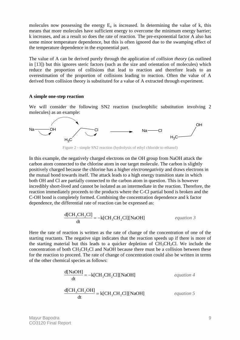
A simple one-step reaction
We will consider the following SN2 reaction (nucleophilic substitution involving 2
molecules) as an example:
CH3
ClNa OH Na Cl
CH3
OH
Figure 2 - simple SN2 reaction (hydrolysis of ethyl chloride to ethanol)
In this example, the negatively charged electrons on the OH group from NaOH attack the
carbon atom connected to the chlorine atom in our target molecule. The carbon is slightly
positively charged because the chlorine has a higher electronegativity and draws electrons in
the mutual bond towards itself. The attack leads to a high energy transition state in which
both OH and Cl are partially connected to the carbon atom in question. This is however
incredibly short-lived and cannot be isolated as an intermediate in the reaction. Therefore, the
reaction immediately proceeds to the products where the C-Cl partial bond is broken and the
C-OH bond is completely formed. Combining the concentration dependence and k factor
dependence, the differential rate of reaction can be expressed as:
]NaOH][ClCHCH[kdt
]ClCHCH[d23
23 equation 3
Here the rate of reaction is written as the rate of change of the concentration of one of the
starting reactants. The negative sign indicates that the reaction speeds up if there is more of
the starting material but this leads to a quicker depletion of CH3CH2Cl. We include the
concentration of both CH3CH2Cl and NaOH because there must be a collision between these
for the reaction to proceed. The rate of change of concentration could also be written in terms
of the other chemical species as follows:
]NaOH][ClCHCH[kdt
]NaOH[d23 equation 4
]NaOH][ClCHCH[kdt
]OHCHCH[d23
23 equation 5

Mayur Bapodra 10 CO3120 Final Report
]NaOH][ClCHCH[kdt
]NaCl[d23 equation 6
Equation 4 has the same form as that of equation 3 as both are starting reactants. Equations 5
and 6 are also the same but this time we are considering the rate of change of concentration of
products with time. As the concentrations of starting materials increase (and hence the
likelihood of a collision leading to a possible reaction) the reaction speeds up resulting in a
greater rate of production of products, hence the sign of k is now positive. No matter how the
rate is expressed the form of the rate law is the same and is a product of the rate constant, k,
and the concentrations of the molecules involved in the reaction. If the reaction involves 2 of
the same molecule, it appears twice in the rate law, leading to a square of the concentration of
that species. The rate law therefore informs us about the mechanism behind an elementary
reaction. Conversely, the mechanism immediately gives us the rate law.
More complex reaction mechanisms
The above treatment is for a simple one-step mechanism. For a more complex reaction
network involving several steps from reactants to products, a differential equation for the
reaction rate can still be derived in this way, but the overall reaction needs to be broken down
into a series of elementary steps, bearing in mind the reversibility of any steps. Each
elementary reaction will have its own energy profile and hence its own activation energy.
Each reaction therefore has a unique value of k. Even for the same energy profile, a reverse
reaction going from products to reactants must overcome a different energy barrier (see
figure 1). Consider the following example reaction mechanism where A and B are molecules
which can react to form C and D, D can then react with B to form G, or E to form F. The
double headed arrows indicate reversible reactions:
k1
k-1
A + B C + D
k3
FD + E
k2
GB + D
Figure 3 - example of complex reaction mechanism
Reaction 1 is reversible, reaction 2 forms a bi-product G which removes D from the system
and reaction 3 forms our desired product F. Ideally, the overall rate of reaction should be
expressed in the concentrations of known species which can be measured, such as the
reactant molecules, or any terminal molecules such as G or F. In order to do this, we need to
first formulate the rate of reaction with respect to each species in the system. The first step is
deciding which elementary reactions produce or consume the species in question. For
example, B is consumed in both reaction with rate constant k1 and k2, but is produced by the
reverse reaction with rate constant k-1. We would formulate the differential equation as
follows:
]D][B[k]D][C[k]B][A[kdt
]B[d211 equation 7

Mayur Bapodra 11 CO3120 Final Report
Similarly, the rate can be formulated for the other species as follows:
]][[]][[][
11 DCkBAkdt
Ad equation 8
]][[]][[][
11 DCkBAkdt
Cd equation 9
]][[]][[]][[]][[][
3211 EDkDBkDCkBAkdt
Dd equation 10
]][[][
3 EDkdt
Ed equation 11
]][[][
3 EDkdt
Fd equation 12
]][[][
2 DBkdt
Gd equation 13
The combination of all of the above differential reactions can then give a picture of how the
rate of reaction looks with respect to a specific species (e.g. a particular reactant or product).
Passing all of these individual equations to a computer math solver could then yield a single
differential equation in terms of one or a few species only, perhaps those of interest or those
that can be easily measured. This differential equation could also be presented graphically,
showing a prediction of the kinetic profile for the reaction, or could be compared against
empirical results to validate or invalidate our proposed reaction mechanism. Slight variations
in the match between the two sets of results could expose overlooked details in our proposed
elementary reactions or perhaps even an entire step. Our methodology will aim to produce
these individual differential equations for a particular reaction.
Use of a stoichiometric matrix
Cardelli [2] proposes a method of deriving these individual ordinary reactions without
explicit knowledge of the elementary reaction mechanisms, via a stoichiometric matrix. If it
is known for each reaction, how many molecules of each chemical species is created or
destroyed, we can build up a matrix as follows:
A B C D E F G
k1 -1 -1 1 1 0 0 0
k-1 1 1 -1 -1 0 0 0
k2 0 -1 0 -1 0 0 1
k3 0 0 0 -1 -1 1 0
Figure 4 – stoichiometric matrix for example reaction

Mayur Bapodra 12 CO3120 Final Report
Each entry in the matrix corresponds to the aggregate number of molecules produced or
consumed in a reaction, negative for consumption and positive for production. For example,
if reaction with rate constant k5 consumed 3 molecules of X but produced 2, the entry for k5
and X in the matrix would be -1.
From this matrix, we can build the rate laws for the elementary reaction steps if we assume
that all reactions are initiated either by collision and subsequent reaction of molecules which
lead to their destruction, or by disintegration of one molecule into several. In both cases, the
reaction occurs through the destruction/alteration of a molecule. If a molecule is involved in
the initiation of an elementary step but is not consumed this method does not work. However,
this is very rare, and even for catalysts (which are never used up by a complex reaction when
considering the overall outcome) there is usually a change in form at the level of elementary
reaction. Each row of the matrix informs us of the molecules involved for a particular
reaction. If we multiply the rate coefficient for each row by the concentration of those species
which are destroyed in the reaction we can define rate laws for our example reaction as:
k1[A][B] for the first reaction
k-1[C][D] for the reverse of the first reaction
k2[B][D] for the second reaction
k3[D][E] for the third reaction
If one molecule of a species is involved as reagents to an elementary reaction multiple times,
it would be treated as another species and that species would be multiplied that many times
e.g. if k5 had a coefficient of -2 for X, it would appear as k5[X][X] or k5[X]2. The derivation
of the rate law matrix from the stoichiometric one is not in Cardelli‟s methodology and he
finds the rate laws in a different way, which no doubt avoids the problem specified above in
assuming elementary reactions occur via the alteration of molecules. Appreciation of this
method would be invaluable for further work and an enhancement of the current
methodology, which has limited universal applicability.
Now we have a rate law matrix and a stoichiometric matrix, the rate law matrix taking the
following form with only one row:
k1 k-1 k2 k3
k1[A][B] k-1[C][D] k2[B][D] k3[D][E]
Figure 5 - rate law matrix for example reaction
A simple matrix multiplication of Rate Law Matrix by Stoichiometric Matrix then gives us a
1x7 matrix with the elementary ODE‟s (equations 7 to 13).

Mayur Bapodra 13 CO3120 Final Report
3. Background – Graph Transformations
This section provides parts of the literature survey conducted for the “Project Plan” as a
summary of existing related work in the use of graph transformations to model chemical
reactions.
Literature survey
[8] gives an excellent overview of basic graph transformation theory. It consists of an easy-
to-follow description of graph transformation systems including the representation of systems
as graphs (type and instance graphs), rules and transformations, constraints and application
conditions. To explain its most basic functionality, a rule first looks for a pattern match for
the left side of the rule in the input graph. Then, edges and nodes that are not in the right hand
side of the rule are deleted, while edges and nodes that are newly created in the right hand
side are placed into the graph. This paper will be invaluable as a reference to basic concepts
throughout the project.
Modelling molecules and reaction networks using graphs is described as a very natural
application by much of the literature [1,13]. [1] and [17] discuss how a form of graphs is
already a fundamental part of organic chemistry, when depicting molecules by their structural
formula. Atoms can naturally be seen as nodes in a graph, with the bonds between them
represented as bi-directional edges. Double bonds and triple bonds could be modelled as two
edges and three edges respectively (as represented in [1]) but this would only be useful if a
reaction involved the breaking of one of the double bonds in one or more of its elementary
steps (this may be useful for the esterification case study).
The problem with this basic approach, however, is a loss of information about spatial
configurations i.e. cis and trans isomers and chirality. Furthermore, the valencies of
individual atoms (the no. of other atoms it can bond to) are not automatically conserved. [5]
offers an alternative approach that should be much more intuitive for chemists. By modelling
the atoms as hyperedges and the bonds between them as nodes, valency and chirality can both
be incorporated into the model. Each hyperedge is typed by atom, allowing for different
numbers of joined nodes, therefore the concept of valency is preserved. The outgoing „bond‟
nodes from a hyperedge are labelled in order to show the three-dimensional ordering (related
to D-glyceraldehyde), and preserving chirality. This is particular important for reactions
where one enantiomer is more reactive in an elementary step, or where only one enantiomer
binds with a particular substrate. This is more prominent in biochemical systems. The
example of Citrate binding with Aconitase is given in [5]. In our two case studies chirality
does not need to be considered as it has no bearing on the outcome of reaction. Therefore the
simpler model may prove sufficient.
From the representation of molecules as graphs, envisioning reactions between molecules as
graph transformations is not a big step. Both [17] and [18] describe how reactions involve the
breaking and creation of bonds in a molecule to transform it into a different molecule. In the
graph, this would mean an elementary reaction step would involve the deletion of edges
(bonds) and nodes not appearing in the right hand side of the rule, and the creation of edges
and nodes that appear on the right hand side of the rule. As nodes and edges can have
attributes, attributes may also be updated during the transformation. Such attributes could
indicate energies of bonds, valencies or other useful information. Another reason why graph

Mayur Bapodra 14 CO3120 Final Report
transformation representations are so natural is their “inherent concurrency” [5]. This is the
ability for these systems to allow simultaneous reactions of different reactants, which is
obviously what happens in real chemistry. Causal dependencies can be monitored along with
conflicts, using critical pair analysis. [17] attributes the strength of graph transformations in
this field to their “pattern handling power”. In any chemical reaction network, involving an
arbitrarily large number of molecules, a multitude of simultaneous reactions are possible.
However, graph transformation rules define the standard reactivity of certain functional
groups. Pattern matching provides a powerful search method for where these rules can be
applied within the network. This will be explored in both our case studies and a more
thorough explanation is giving in later sections of this report.
[5] explains how graph transformations work in detail, by summarising the so-called double-
pushout approach. The left side and right side of the rule span show how the molecule will
change, whereas the gluing graph between the left and right hand side simply indicates which
elements are involved (“read”) in the rule, but not consumed. In the “toy” model of artificial
chemistries given in [1] the essential idea is the same, but the gluing graph is labelled the
context. The visualisation is also much more attuned to the structural formula representation
used by chemists – atomic/group nodes are just labelled by element symbols and the edges
replaced by standard bond representations (with double and triple bonds preserved). Although
this may be more intuitive for chemists, it does not allow us to easily show attributes of nodes
or edges, and also may seem alien to the way the graphs will look in their eventual
implementation using tools such as AGG. Using standard graph representations should be
easy enough to understand so the further simplifications in the toy model are not necessary.
[5] suggests 3 types of rules in any graph transformation system. Symmetry rules are useful
for the hyperedge model. Although chiral molecules cannot rearrange their spatial
configuration with respect to the other groups around the chiral carbon centre, the bond
connected to this carbon can itself rotate, meaning the groups can change position. So that
this is not considered a separate molecule, equivalence rules can be set up. Expansion rules
allow us to expand atoms grouped together in one node/hyperedge (usually for simpler
representation) into their full expanded graph. This is necessary if at some point in the graph
the details of the group become important e.g. one of the atoms is involved in a reaction.
Again, this contracted representation is familiar for chemists, who often contract large groups
in structural formula when their exact spatial details are not contextually important. Reaction
rules define the change of groups. Our model should definitely incorporate the second and
third types of rules, and consider the symmetry rules if the chirality preserving hyperedge
model is used. [5] provides some other invaluable information about how graph
transformation theory can be applied to reactions, and how atoms can be traced throughout
the reaction and will serve as good reference material throughout the project.
Stochastic graph transformation systems and rates of reaction
[10] and [11] are excellent references explaining the extension of a graph transformation
system to a stochastic graph transformation system. Given a start graph and a graph
transformation system, a labelled transition system can be deduced which shows all the
possible states (graphs) possible. Applied to a reaction network, each state would represent
all the species (reactants, products, by-products and intermediates) that would result from
applying the graph transformation rules. Labels from state to state can be assigned attributes
such as a probability of reaction. This is analogous to the rate of the transformation from one
step to the next, hence essential to our derivation of the overall rate of reaction. [10] provides
all the necessary definitions and procedures needed to convert a stochastic graph

Mayur Bapodra 15 CO3120 Final Report
transformation system to a Continuous Time Markov Chain, which then allows the
application of stochastic temporal logic to deduce long-term non-functional stochastic
properties of the system. Equivalence rules can be set up which check for certain properties
of the system at any point during the progress of the simulation, thereby allowing us to
monitor the presence of molecules for example. Querying the system at regular intervals can
then allow us to effectively measure properties proportional to the concentration of chemical
species. Paper [10], demonstrates the application of stochastic graph transformations to P2P
networks. Although the model is simpler (in that the rates are more easily assigned) the
example will be invaluable in understanding how stochastic systems are applied. As the
theory behind stochastic graph transformations (Continuous Time Markov Chains, Q-
incidence matrices, Stochastic Temporal Logic) can be quite difficult to grasp, both of these
papers will be useful to return to.
In deciding the rates of elementary steps, paper [1] provides a very good starting point. As
discussed earlier, the Arrhenius equation relates the change in energy between reactants and
products with a rate of reaction. [1] discusses a refinement where instead of entire molecules,
just the energy of hybridised orbitals involved in the reaction are considered. For complex
reactions such as case study 2 we can follow the methodology described in [1] and automate
the procedure of assigning energies by looking at recurring sections of molecules
(characterised by different hybridised orbitals) rather than entire molecules. This
generalisation step would avoid having to manually determine and assign energies for the
high number of possible species involved in the reaction (i.e. chains of many different
lengths). It can incorporate more complicated electronic distributions accurately into the
model, such as π-stabilisation where adjacent π-bonding orbitals can overlap in a molecule,
lowering their overall energy and making them more resistant to breaking and therefore
reaction. [1] also describes how this method accounts for regioselectivity within a molecule
i.e. if there are two places where a rule can be applied, calculating energies would force the
rate of reaction at one site to be realistically higher than the other. [1] actually goes on to
suggest that the calculation of energies could be used for stochastic simulations of reaction
networks using the Gillespie algorithm. The background theory and ideas presented in this
paper could be utilised in the project, possibly for future iterations.
There are other methods in the literature that are used to model stochastic systems. [2] and
[14] both use process languages to specify the reaction rules and to derive useful properties.
Cardelli‟s paper [2] is particularly useful as it sets out to achieve what this project does using
stochastic process algebra, namely CCS and CGF. While this approach is probably more
intuitive and precise for computer scientists, it loses its appeal for chemists due to its
technical complexity. The visual graph representation is much more useful in this respect
because the components are easily recognisable to chemists. The content of the paper is quite
technical and without a background in logic and automata course requires substantial
background reading to understand fully. The paper is therefore currently of limited use.
Nevertheless, it would be highly advisable to understand Cardelli‟s approach, in order to note
his assumptions and the way in which he assigns rates to elementary reaction steps. For this
reason, a quick overview of π-calculus (provided by [15]) and subsequent research into CCS
still needs to be undertaken.
Implementation tools
AGG [19] is widely used by the graph transformation academic community. A brief
description of its utilisation to a chemical reaction setting is given in [5]. AGG does have
several limitations for our purposes though. Firstly, it cannot be used for stochastic

Mayur Bapodra 16 CO3120 Final Report
simulations. To obtain stochastic data, a combination of PRISM and GROOVE (as described
in [10] and [11]) could be used. [6] also provides a very thorough presentation of FERN, a
Java framework that can be used for stochastic simulation. The API seems fairly
straightforward. It does not however provide its own visualisation module. AGG also has its
own Java API and a combination of the two tools could be coordinated to fit the project‟s
needs. Further investigation of [6] and [19] will be necessary to achieve this. An appealing
feature of [6] is that it provides implementations of several stochastic simulation algorithms,
namely the Gillespie algorithm, extended Gillespie algorithm and a tau-leaping algorithm.
The framework applies the most appropriate algorithm depending on the speed of the reaction,
and can even change dynamically during runtime.
Other limitations of the software should also be considered before using AGG such as
minimum requirements, known bugs and elements of graph transformation theory that are not
implemented (such as the ability to input hyperedges). The user manuals, bug reports and
examples which can be found at [19] should be reviewed before/while using the tool.
Consideration for more complete modelling
Despite being an overview paper that has little relevant technical content, [18] does
illuminate some interesting points to consider if we are to progress to a more complete model
of real chemistries. In particular, “Global Context Sensitivity” is discussed. This states that
physical properties play an important role in chemical reactions, such as temperature, solvent,
viscosity, catalysts and radiation to name just a few. A graph transformation model may be
limited in its ability to incorporate such factors. This should be taken into account in the final
stages of the project. “Local Context Sensitivity” considers for example the “three
dimensional conformation of reactive groups” of a molecule and how this affects reactivity.
Large groups for example may block collision with incoming molecules, thereby hindering
reaction rates.
While a complete and accurate model is impossible for the scope of this project, it would be
interesting to consider some of these factors, in particular temperature as the Arrhenius
Equation is temperature dependent. The quality of results from the model compared to
empirical results may prompt further investigation into these factors towards the end of the
project, time permitting. We will return to this paper for background knowledge at this stage.
Graphs and type graphs
The graph transformation theory covered in this section provides a non-technical overview of
the theory necessary to understand our methodology. For a richer, more mathematical
discussion of the theory presented here, with formal definitions, please refer to [4], [5] and
[8], of which the following is a summary.
Graphs are composed of a set of nodes and a set of directed edges. Each edge has a source
and target node. Formally, a graph can be represented as:
G = (V, E, s, t) equation 14
…where G is a graph, V is the set of vertices (or nodes), E is the set of edges, and s and t are
the source and target functions respectively (s,t : E V).

Mayur Bapodra 17 CO3120 Final Report
A typed graph is much like a UML class diagram, in that it specifies the allowed types
(analogous to classes) of nodes and edges, and also the allowed relations between different
nodes and edges. A type graph can also be formulated in the same way as equation 14:
TG = (VTG, ETG, sTG, tTG) equation 15
A graph is typed if it conforms to the specification laid out in the type graph, and is
represented formally as:
GT = (G, type) equation 16
… which specifies that a typed graph consists of a graph and a graph morphism, which is
essentially a function, which maps the graph to the type graph, type : G TG. A graph
morphism is a combination of two functions; one that maps all vertices from one graph to
another, and one that maps the edges in the same way. All nodes and edges must be instances
of the node types and edge types specified in the type graph. The graph as a whole may be
considered an instance of a type graph, just as in UML an object is an instance of a class. As
an example, consider the following simple type graph:
Figure 6 - example type graph
This specifies that the red node can only connect to a black node via a purple edge, and the
blue node can only connect to a red node via a green edge (note the direction of the edges).
Just like UML class diagrams, cardinalities can be specified on relations between nodes
through their edges. Every blue node must have 1 or 2 red nodes connected to it. Every red
node must have 1 blue node connected to it. The relation between the black and red node is
unconstrained, i.e. there is a zero to many cardinality. As there is no edge between the blue
and black node, the blue node must never be connected to the black one. A red node can be
connected to no more than one other red node (including itself). An example of a valid typed
graph over this type graph is given in figure 7:
Figure 7 - example typed graph

Mayur Bapodra 18 CO3120 Final Report
Graph transformations
A graph transformation (also known as a rule or production) is a graph morphism that is used
to specify how a graph can change. It is usually specified in the following way:
Figure 8 - definition of a graph transformation (DPO)
This is known as the double pushout approach (DPO) construction. L is the left-hand side of
the rule and specifies the preconditions for the application of a rule. It is itself a graph which
contains nodes and edges. K is the gluing (or sometimes called the context) graph. This
specifies which nodes and edges in L are unchanged by the rule (i.e. “read” only). R is the
right-hand side of the rule and specifies the postconditions for the application of the rule.
Nodes and edges in L have an identity and these are mapped to nodes and edges in K and R,
unless of course R introduces a new node or edge, in which case it will not have an identity.
In order to perform a transformation on a given graph, there must be a match for the nodes
and edges in L within the graph i.e. there must be an injective morphism (every member in L
must be mapped to a unique member in the graph). There can be more than one such match,
in which case one is non-deterministically chosen for the transformation (AGG allows
interactive matching which allows you to select which match to perform the transformation
with). Once a match is found, i.e. a copy of L is found in the graph, the nodes and edges not
in K are deleted, and the new nodes and edges in R are copied into the graph. This can be
represented pictorially as:
Figure 9 - definition of graph transformation with match
m, k and n all depict the embedding (injective morphism) of L, K and R respectively into G,
D and H, the instance graphs. G is the graph before the transformation, D is the graph after
the non-preserved nodes have been deleted, and H is the graph after the new elements in R
have been copied over.
The subgraphs that constitute the left and right hand sides of a rule must also conform to type
graph specifications. An example rule for the type graph given in figure 6 is:
Figure 10 - example rule 1
L K R
G D H
L K R l l
r
l
l l
r
l
m
l
k
l f
l
g
l l
n
l

Mayur Bapodra 19 CO3120 Final Report
Figure 10 shows only the left and right hand side of the rule. These diagrams were produced
using AGG (a graph transformation tool), which does not require the input of a gluing graph,
as this is inferred from the left and right hand sides. The gluing graph here would be the red
node (1), which is the only node preserved by the rule. This rule essentially just deletes a
black node, and its corresponding edge, connected to a red node. If this rule is applied to the
graph in figure 7, we would get the following:
Figure 11 - rule 1 applied to example graph in figure 7
While there are three matches for the left hand side of the rule, there is only one valid match.
Deletion of the second black node, connected to two red nodes, would lead to a violation of
the dangling condition. The two remaining matches select either one of the red nodes with the
black node. For either of these, if the black node and one edge are deleted, another edge is
left without a target node, hence a dangling edge. There are two ways to overcome this, either
to delete the dangling edge, or disallow transformations that lead to a dangling edge (AGG
allows the setting of this as an option). In our case, we do not delete dangling edges, hence
there is only one valid match.
Critical pairs
The theoretical background presented here is a summary of the chapter on critical pairs in [4].
A critical pair refers to a pair of rules where one rule could potentially affect the application
of another. There are two main types of critical pairs: conflicts and causal dependencies.
Conflicts refer to parallel dependent pairs of rules, where the application of one rule could
disable the application of another. Consider a graph, G, with the possible application of rule
p1 or rule p2:
Figure 12 - parallel independence of rules [4]

Mayur Bapodra 20 CO3120 Final Report
If the above confluence is possible, rules p1 and p2 are parallel independent. However, if the
transformation p1 on graph G creates a graph H1 such that p2 can no longer be applied, or p2
on graph G creates a graph H2 such that p1 can no longer be applied, the two rules are parallel
dependent and in conflict. We can check for such a conflict by depicting the double pushout
construction for each rule.
Figure 13 - double pushout depiction of parallel independence [9]
For parallel independence, each rule must not delete nodes and edges needed in the left hand
side of the other rule. In other words, D2 (the gluing graph which specifies which nodes and
edges are not deleted by rule p2) must contain L1, and D1 must contain L2. Another way of
considering this is to look at the union of the left hand side of both rules. There will be a
number of graphs satisfying this union, each graph depending on exactly how the union takes
place. If in any one of these unions, the intersection of the two left hand sides is not in the
gluing graph of both rules (K1 and K2) the rules are in conflict.
For sequential dependence, we consider the following construction:
Figure 14 - double pushout depiction of sequential independence [9]
Rule p1 has been reversed. If the order in which p1 and p2 are applied affects the overall
outcome of the application of both rules, there is sequential dependence. Here we consider if
D2 contains R1 instead of L1. If we have a reaction rule p1 such that it creates the graph in the
LHS of p2, L2 will be in R1 but will not be in D1. Since p1 creates L2, L2 should not exist in
this gluing graph (i.e. before p1 is applied). This is identical to saying that for some
intersection of R1 and L2, K1 will not contain this intersection as some nodes and elements in
L2 will not have been produced yet. The intersection of R1 and L2 should be in both K1 and K2
for sequential independence. Therefore, in this case, we have a critical pair denoting
sequential dependence.
R1 K1 L1 L2 K2 R2
H1 D1 G D2 H2
p1 p2
L1 K1 R1 L2 K2 R2
G D1 H D2 G’
p1 p2

Mayur Bapodra 21 CO3120 Final Report
Stochastic graph transformations & reaction networks
Although stochastic techniques were not utilised in this project, considerable time was spent
studying and understanding their application to chemical kinetics in the first term. As such, a
very brief summary of their use is given here, gathered from [10] and [11]. As mentioned in
the introduction, stochastic simulation is an alternative and better studied approach to
producing reaction kinetic data. There are a number of differences between this approach and
ours. While ours aims to produce equations, simulations produce quantitative data. This
quantitative data depends on the circumstances under which the simulation was run, and also
chance. Simulations consider every possible change from one molecule to another by a
reaction in an atomic way, considering each one a unique transformation. Differential
equations, however, essentially average all of these unique transformations into one overall
rate law for that reaction. The stochastic simulation technique described below requires the
input of a reaction mixture (many of each molecule) as the first state of a labelled transition
system. There are scalability issues here in the number of instances of each molecule possible
before the simulation can no longer run efficiently. Differential equations overcome this as
generally only one instance of each molecule involved in each elementary reaction is
necessary. Both of these approaches should be considered as complementary and further
work would look at the connection between them. Therefore, an understanding of the theory
behind stochastic graph transformation systems is very useful for the project.
While a graph transformation system describes the functional, behavioural aspects of a
system, adaption of this to a stochastic graph transformation system can inform us of non-
functional properties of the same system. The speed at which reactions occur is one such non-
functional property. To derive kinetic information about a particular complex reaction, we
would first need the rules that make up the elementary reactions for the system, and a type
graph to which all rules and graphs must conform to. We can derive a labelled transition
system from these rules if a start graph is used to apply these rules to. The start graph
describes the initial state of the system. In our case the start graph would be the starting
material molecules for the reaction.
We can describe the resulting labelled transition system as a labelled transition graph, where
each graph is reachable from the start graph through the consecutive application of rules,
starting at the start graph. Each transition is labelled with the rule name. This system now
describes the entire reaction network, with intermediates as graphs in the labelled graph
system and rules as the transitions between these graphs.
To progress from this transition system to a stochastic graph transformation system we need
the notion of a Q-matrix and Continuous Time Markov Chains (CTMC‟s). A Q-matrix
(without formal mathematical notation, which can be found in [10]), is a transition rate matrix
which describes essentially the probability that a particular transition will occur in the
labelled transition system, transforming one graph to another. In chemistry, this is analogous
to the rate constant, k, for an elementary reaction, which transforms one set of molecules to
another. Just as the Q-matrix value describes some inherent probability of transition from one
graph to another, k is an inherent probability of reaction for a particular elementary reaction.
The usual concentration dependence that the speed of reaction has is incorporated into the
transition system model elsewhere; the more molecules there are of a particular type required
in a reaction, the more likely a transition of that type will fire in any given interval if we look
at the system as a whole.

Mayur Bapodra 22 CO3120 Final Report
Each entry in the Q-matrix describes the transition rate from one state to another. The rows
and columns are both elements from the set of possible states for the system to be in. Each
row must sum to 0 (a necessary normalisation prerequisite for Q-matrices). If a transition
from one state to another is impossible, the Q-matrix entry where they intersect is 0. The rate
from one state to the same state is usually where a negative value is inserted to normalise the
matrix. For example, if A, B and C are intermediate states in a reaction, the Q-matrix might
look as follows:
A B C
A -5 5 0
B 3 -11 8
C 1 0 -1
Figure 15 - example Q-matrix
Here we see that A can go to B but cannot go to C. B can go to A, but is more likely to go to
C. C can go to A, although it is not very likely, but not B.
From the labelled graph system and the Q-matrix, we can define a Continuous Time Markov
Chain (CTMC). The CTMC is a random process, which describes the state of a system
indexed by some t. In our case, t is time, since we are considering the progress of a reaction
with time. If t is from a continuous set (as it is with time), we are describing a continuous
time process as opposed to a discrete time process. The “continuous time” in CTMC refers to
this. The CTMC is discrete-state since the intermediate graphs are the result of concrete,
finite rule applications. The current state in the CTMC only depends on the previous state.
The Q-matrix, along with the finite states provided by the labelled graph system, defines a
CTMC in the following way. If the Q-matrix entry is greater than zero for any 2 sets of states,
s and s‟ (provided s ≠ s‟), then a transition from s to s‟ occurs. So in our example Q-matrix
above, if we start with A, A can progress to B. If there is more than one possible transition,
however, a “race” between the possible transitions occurs, with the probability of any
transition winning and therefore firing being the value of that entry in the Q-matrix divided
by the total non-negative values in that particular row of the matrix (also given by the
negative of the value for the s,s entry in the matrix). For example, once at B, we can return to
A (with a value of 3) or progress to C (more likely, with a value of 8). The probability that B
A occurs is 3/11, and the probability that B C occurs is 8/11.
Another important note about the CTMC is that the transition delay is exponentially
distributed with rate –Q(s,s) i.e. the probability that a state, s, will change within time t is the
same at any time and depends on the sum of the entries for any row (i.e. state) of the Q-
matrix. The memoryless property of exponential distributions is particularly suited for
chemical reactions, as it indicates that the proportion of molecules to undergo a particular
elementary reaction in time interval, t, is constant. Again, this indicates an inherent reactivity
of the molecules involved in an elementary reaction. As the sum of the rate constants for all
outgoing reactions determines how fast a particular intermediate molecule will react and be
used up, this is intuitively correct. These same rate constants determine the values in the Q-
matrix. The changing concentration of species needed for a reaction to occur will have an

Mayur Bapodra 23 CO3120 Final Report
effect on the overall speed of reaction, but the rate constant and inherent reactivity of the
molecules needed for a reaction should never change (assuming a constant temperature).
The stochastic graph transformation system then, attributes to each rule (i.e. transition in the
labelled graph system) “an exponentially distributed delay of its application” [10], which is
derived from the Q-matrix (details of how to do this are given in [11]). In chemical reactions,
this is proportional to the value of the rate constant for a particular reaction. Such a system
can be implemented using a tool chain such as AGG for rule specification, and GROOVE and
PRISM for specifying the Q-matrix and running the stochastic simulation. Continuous
Stochastic Logic (CSL) can then be used to query the stochastic system. This involves setting
up atomic propositions which question the probability of certain events occurring (e.g. is the
probability that there are 1000 molecules of intermediate molecule C present after 20 time
units 0.1?) either throughout the time of the simulation or at long-term steady state (i.e. the
end of the reaction). Using appropriately designed queries, a value (actually a probability)
proportional to the number of molecules of each species can be ascertained throughout the
simulated reaction. If we assume a constant volume, this is proportional to the concentration
of each species. A graph of concentration against time for each species can then be plotted
and checked against empirical lab results.
This was a very brief and non-mathematical overview of stochastic graph transformation
systems. More details can be found in [10] and [11].
As stochastic simulations give us numerical, quantitative data that can be directly compared
to existing experimental data, it may be reasonable to ask why ODE‟s are necessary at all.
The ODE‟s give us a direct insight into the overall reaction mechanism for a complex
reaction. A plot of the combined ODE‟s compared to experimental data may reveal drastic
differences, which may be due to an inadequately proposed mechanism (i.e. omissions or
inclusion of reactions that never occur), or highlight interesting physical properties of a
reaction e.g. temperature dependence or dependence on molecular size or spatial
configuration. While the methodology developed in this project does not come anywhere
close to incorporating such physical influences on a reaction, the knowledge of their presence
alone is invaluable.

Mayur Bapodra 24 CO3120 Final Report
4. Molecular Representation Using Graphs
So far this report has focused on background and related work done in this field. The
following is an account of how this was used in this project. First we focus on the use of
graphs to represent molecules and their reactions, and then describe the step by step
derivation of ordinary differential equations for a reaction, using the concept of critical pairs.
This is followed by a description of the implementation of this methodology using 3rd
party
and newly developed tools. Our two case studies test the methodology and its implementation
for a finite reaction mechanism.
A type graph is extremely important when representing molecules using graph
transformations. A type graph captures the necessary rules to restrict the bonding of atoms,
their valencies (the total number of bonds a particular atom is allowed to have) and any other
idiosyncrasies of molecular chemistry. During the initial stages of the project, several type
graphs were experimented with. This section gives an account of the evolution of these
approaches through three main stages.
1st attempt
Because molecules consist of atoms and bonds that connect two atoms, a first intuitive
representation of molecules might consist of atoms as nodes and bonds as edges that directly
connect them. A first approach followed this intuition and produced the following type graph
(for all atoms in the esterification example):
Figure 16 - esterification type graph, 1st attempt
The structure of the type graph is quite complex. Just as with UML class diagrams, we can
see the use of inheritance in this type graph. All of the atoms are subtypes of the “atom”
supertype. C, H and H+ are all subtypes of “R” (used in organic chemistry to designate an
arbitrary hydrocarbon chain), which in turn is a subtype of “atom”. A bond between atoms
must consist of a pair of edges, one in each direction. As edges are directed, making each
bond a pair of oppositely directed edges avoids the added complication of specifying a
direction between each pair of atoms, and allows the use of a supertype, generic atom to

Mayur Bapodra 25 CO3120 Final Report
specify all allowed connections. This is why all bond edges are directed to the central “atom”
supertype. The cardinalities of the bond edges specify the valencies for each atom. For
instance, the O type must have 2 outgoing edges to other atoms, and 2 incoming edges,
therefore specifying that each O atom must have 2 atoms connected to it at all times. The
“atom” supertype has a connection to itself. This is to allow connections between atoms.
While the edges from the subtype atoms to the supertype “atom” should already assume this
possibility, AGG did not allow it unless the “atom” to “atom” edge was added. Charged
atoms were included separately as they have different valencies to their non-charged
counterparts. O+ can have 3 connections for example, whereas neutral O can only have 2.
In producing a graph over the type graph above, in AGG the type graph must be enabled.
There are two options for enabling the type graph – with both minimum and maximum
cardinalities enabled, or just the maximum. With the minimum enabled, this minimum is in
effect throughout the lifetime of the graph, even when rules are being applied, and as most
rules involve deletion of an edge before re-adding another, this minimum may be violated
making the rule inapplicable. Therefore, for all type graphs, we only enable the maximum
cardinalities of the type graph. Figure 17 shows an example of a graph that conforms to the
type graph of figure 16. These are the starting materials in the esterification reaction studied
in this project:
Figure 17 - esterification start graph, 1st attempt
The leftmost molecule is a carboxylic acid, ethanoic acid. Between the C on the right and the
upper O, there are 4 edges in total, therefore 2 bonds. Under this type graph, this is how a
double bond is represented. The small molecule is TsOH, an acid catalyst in the reaction.
Here, we have encapsulated the complicated internal structure of p-Toluenesulfonic acid as a
single TsO node, as this internal structure is not important to the reaction; only the attached H
atom has any significance. The molecule on the right is the alcohol (ethanol) which reacts
with the ethanoic acid to eventually form an ester.
As the minimum cardinalities are disabled for the graph, it is entirely possible that through
the course of the reaction certain required conditions may become violated, in particular the
fact that each bond must consist of two edges. This is particularly important for critical pair
analysis, which we will discuss later, where we look for critical overlappings of nodes and
edges between a pair of rules. When we specify rules, we can carefully control their outcome
through the left and right hand sides. Critical overlappings however are extracted from all

Mayur Bapodra 26 CO3120 Final Report
possible permutations of an embedding of the two rules into one graph. To ensure all of these
permutations conform to rules not specified in the type graph, we can use constraints.
Constraints are specified for an entire graph grammar (rules and start graph). An atomic
constraint consists of an atomic proposition, and one or more conclusions that must be true if
the proposition is true. For example:
Atomic proposition: Atomic conclusion:
Figure 18 - atomic constraint for 1st attempt type graph
This atomic constraint states that whenever one atom is connected to another by an edge,
there must be an accompanying edge in the opposite direction. A constraint can be
formulated from many individual atomic constraints using Boolean logic. Constraints
specifying the necessary presence of a situation can be expressed by leaving the atomic
proposition empty and specifying an atomic conclusion. This means that the conclusion must
always be true. To specify required absence, a constraint that falsifies such an atomic
constraint must be defined.
While this was an extremely intuitive type graph, which could easily be understood by both
chemists and computer scientists, there are some drawbacks because of its simplicity.
Primarily, the dangling condition (described earlier) can easily be violated in the specification
of a rule unless extended local context is given in that rule. For example, if a rule specified
that one of the bonds of the C=O double bond in ethanoic acid (figure 17) should break to
leave a single bond, with C becoming C+, we would need to break the other bonds this C has
and reform them with the C+. If the rule only included the C which actually changes, and left
out the local context, the rule would become inapplicable as the dangling condition would be
violated when C changed to C+. Generally, to specify reactivity that is as general and widely
applicable as possible, rules should include only the functional groups that are affected by
rules, and avoid local context. A way around this for this particular type graph, would be to
split rules (as can be seen for rules entitled Step4a and Step4b, in file
“esterification_attempt1.ggx”), but this adds unnecessary complication to the grammar.
2nd
attempt
A second attempt looked at incorporating a hyperedge treatment. AGG does not allow the use
of hyperedges. However, they can be simulated using bipartite graphs, as carried out in [5]. A
hyperedge is an edge that connects more than two nodes. The nodes that a central hyperedge
connects can be ordered thereby some semblance of 3-dimensional spatial configuration is
preserved. This is an extremely useful property for the reactions of chiral molecules where
only certain enantiomers (3-dimensional configurations) undergo reactions. For our case
studies, chirality was not relevant. However, this representation also enables an easy way of
limiting the number of bonds each atom is allowed, hence establishing valency maximums.
CH4 (methane) would have the following hyperedge representation:

Mayur Bapodra 27 CO3120 Final Report
Figure 19 - hyperedge representation of CH4
Contrary to the 1st model, atoms are now (hyper)edges, and bonds are nodes. The green
hyperedge is the central carbon atom, and the blue hyperedges are the bonded hydrogen
atoms. The black nodes represent a bond. Hyperedges of carbon type can connect four such
nodes and hydrogen only one. This restriction information would be in the type graph for this
hypergraph. The bipartite graph simulation of this would have the following form:
Figure 20 - bipartite graph representation of CH4
The hyperedges are simply represented as a special type of node in AGG. The resulting form
of the graph is very similar in appearance to the hyperedge approach.
The type graph for esterification in this model is given in figure 21. The corresponding
starting materials (analogous to figure 17) are given in figure 22. The type graph in figure 21
is considerably simpler than the type graph in figure 16, for the previous model. However,
there are again drawbacks with this model. While the number of bond nodes each atom node
can connect to is appropriately limited, the opposite is not true. From the type graph it is clear
that each bond node could have several atoms nodes attached, a maximum of 2 for C, 2 for O,
2 for O+
, 2 for H etc. To prevent this, a great number of constraints would need to be added to
the grammar, ensuring every possible combination of atoms at a bond node is accounted for.
This would increase the complexity of the grammar, and we can speculate that checking this
many constraints could make critical pair analysis or rule applicability analysis perform much
less efficiently. In addition, the generic bond nodes that are used throughout each molecule
would increase potential inclusions to check for during critical pair analysis. Embedding one
v1 v2
v3
v4

Mayur Bapodra 28 CO3120 Final Report
rule into another, both of which use these nodes heavily, equates to far more possible
embeddings to check through.
Figure 21 - esterification type graph, 2nd attempt
Figure 22 - esterification start graph, 2nd attempt
3rd
attempt
After many experiments and modifications of the two type graphs given above, a final type
graph was settled upon. This extends the bipartite graph idea, but solves the problem of
spurious connections to each generic bond node, by introducing more detail to this node.
Each generic bond node is now a pair of atom-specific bond nodes. Each atom node can have
a certain no. of atom-specific bond nodes (thereby introducing valency in the same way as the
bipartite graph system), and each atom-specific bond node can only be connected to one other
atom-specific bond node. This is specified through a combination of the type graph and
additional constraints. As edges are directed, there must be a simple way of determining the
allowed direction between each possible pair of atom-specific bond nodes. It was decided that
the relative electronegativities (the ability of an atom to draw electronic charge towards it) of
each atom would determine this direction. As O is more electronegative than C, the direction
of the edge would go from the C bond node to the O bond node. The final type graph used in

Mayur Bapodra 29 CO3120 Final Report
our case studies is given in figure 23. An instance of this, esterification starting materials as
per the two previous examples, is given in figure 24.
Figure 23 - esterification type graph, final version
Figure 24 - esterification start graph, final version
Although the graph is much bigger, involving far more nodes, this representation solves
many problems. As mentioned in the appraisal of the plan (see page 73), many changes to the
representation came about through problems with the case study or implementation. This
representation led to far fewer inclusions at the critical analysis stage (explained in
“Methodology”) due to the lack of generic or non-atom-specific nodes and was therefore
selected for the project. A slight modification of this type graph was used for the second case

Mayur Bapodra 30 CO3120 Final Report
study, but this will be covered in more detail when describing that case study. Note that the
C-C bond in both of the larger molecules has two edges (in opposite directions) between the
bond nodes. This is because the C-C bond is symmetric in terms of electronegativity, so this
added convention is useful. This can be enforced using a constraint in the same way that all
bonds had to consist of two edges in the first attempt type graph (see figure 18).
As explained, additional constraints were also necessary to limit the number of edges each
bond node could have. Each bond node should only have 2 connections (except for
symmetric bonds). Atomic constraints took the following form and had to be specified for
each permutation of 3 atoms, and then these had to be declared to be false in an overall
constraint:
Atomic proposition: Atomic conclusion:
(empty)
Figure 25 - example bond node constraint for final type graph
As expected, this was very cumbersome and led to a total of over 40 such atomic conclusions.
For a more complicated reaction system involving more varied elements these constraints
would grow to be extremely difficult to define by hand. This was a major drawback of the 2nd
attempt, and now this one. However, this drawback is fixed in the revised iteration of this
type graph used for the second case study, using inheritance in the type graph and constraints.
When the esterification type graph above was designed, after some discouraging results, it
was unclear as to the effects of inheritance on AGG‟s implementation of critical pair analysis
and was therefore avoided. Later, whilst working on the second case study, we speculated
that inheritance should only cause problems with the critical pair analysis if generic
supertypes were used in the definition of rules, and not in type graphs or constraints, as these
are merely checking mechanisms for the validity of a graph. If inheritance is used in a rule, at
critical pair analysis, the supertype node can be substituted for every subtype in the concrete
overlapping graph, leading to a possible explosion in the number of inclusions to check. It is
not even clear as to how inheritance in rules is treated by the critical pair analysis engine of
AGG.
While the improved revision is discussed in more detail later, the type graph above gives the
general idea of our approach, using two bond nodes for each bond. This is still a very
intuitive molecular representation for chemists. The two bond nodes could even be visualized
as the pair of electrons needed to form a directed bond between two atoms.
Mayur Bapodra 31 CO3120 Final Report
5. Methodology
A background on critical pairs was given in “Background – Graph Transformations”. The use
of critical pairs for deriving ODE‟s presented below is adapted from [9].
Use of critical pairs
The concept of critical pairs can be used to determine which molecules are consumed by
which reactions within a network of reactions. To do this, first we need to establish the
reactions as one set of graph transformation rules and the molecules (starting materials and
intermediates in the reaction) as another set of identity (or identic) rules and check for critical
pairings between members of these two sets. An identity rule is one in which the left hand
side (LHS) of the rule and the right hand side (RHS) are identical. Hence, it can only be
applied to a graph if the LHS of the rule is present within that graph, and its application does
not change this graph. As such, identity rules are generally used to check for the presence of
certain subgraphs within a graph.
Consider a reaction rule p1 which defines a transformation that breaks bonds (i.e. in our graph
representation of molecules, deletes edges and bond nodes) that are present in a molecule, m.
Let us create an identity rule for m, called m1. If we were to check for critical pairs between
p1 and m1, all overlappings (or unions) of the LHS of rule p1 and LHS of m1 would need to be
constructed. If in any of these overlappings, the nodes and edges that are deleted by p1 are
also in m1, we have a critical pair as the application of p1 at this particular match would mean
m1 could no longer be applied, since the molecule would be changed by p1. Notice that we do
not need to consider the gluing graph for m1 as per the construction in figure 13 because for
an identity rule, the LHS, gluing graph and RHS are all identical. Checking the LHS alone is
sufficient. What the check actually equates to however, is the fact that the intersection of the
LHS of m1 and p1 is not in the gluing graph of p1, since p1 deletes some of these nodes and
edges. In summary then, a critical pair consisting of a particular reaction rule and molecular
identity rule signifies that that reaction consumes that particular molecule.
In a similar fashion, the concept of sequential dependence (see figure 14) can be utilised to
find which reactions produce molecules. If we have a reaction rule p1, and a molecular
identity rule, m1, such that p1 creates the molecule in the LHS of m1 at some stage of the
reaction mechanism, for some overlappings of R1 (from p1) and L2 (from m1), some nodes
and edges in L2 will not be in the gluing graph of p1, since this reaction rule creates L2. All
nodes and edges in R1 however will be in L2, and therefore D2 (since L2, D2 and R2 are
identical). In other words, for a reaction p1 that produces a molecule in the LHS of m1, p1 can
be applied before m1, but m1 cannot be applied before p1. This is the condition for sequential
dependence.
These two categories of critical pairs give us the crucial elements necessary to derive ODE‟s,
since to do this, all we need is information regarding in which elementary reactions chemical
species are produced or consumed. Parallel conflicts and sequential dependencies between
reaction rules and molecular identity rules give us this information.
What follows is an account of how this theory is incorporated into an overall methodology in
deriving ODE‟s. There are 10 steps, each of which is covered in detail. To test the
methodology, these steps were implemented with the aid of the critical pair analysis tools of

Mayur Bapodra 32 CO3120 Final Report
AGG with some additional classes/modifications for added efficiency, automation, and the
eventual output of ODE‟s. The details of how this was achieved are given in the next section,
“Implementation”.
Step 1: Specification of reaction rules and starting materials in AGG
Using AGG, and a suitable graph representation of molecules, specify all general
reactivity as graph transformation rules, including all relevant reverse reactions.
Define the starting reactants as the start graph for the grammar. Each starting
chemical species should also be added as the LHS and RHS of identity rules.
At this stage, the reaction rules must be as general as possible, possibly at the level of
functional groups only. A functional group is the part of a molecule that undergoes a reaction.
For example, in acid-catalysed esterification, the C=O double bond undergoes protonation at
the start of the reaction. For a general reaction rule, we would only include the C=O part of
the molecule in the LHS of the rule. The reason for this is so that the rule can be applied at a
later stage in the reaction, for a possibly unknown intermediate. If the rule is too specific at
this stage, the reactivity of this intermediate is missed, and the ODE‟s will not be accurate.
This is particularly important for chaining reactions, where the intermediates are essentially
too numerous to define or even count. The reactivity of each of these needs to be considered
in an automated way.
Reaction rules should be labelled Step1, Step2 etc. while molecular identity rules should be
named by the molecule they represent in the textual form of the structural formula of the
molecule. For example, ethanoic acid with the following form, would be CH3COOH:
O
OH
H
H
H
Figure 26 - structural representation of ethanoic acid
This is a convention that is necessary for the extraction of ODE‟s in recognized chemical
forms at a later stage.
Step 2: Application of reaction rules to the start graph to obtain intermediates
With the graph grammar defined in step 1, attempt to apply all general reaction
transformations to the start graph. For each resulting graph, add any new
chemical species as new identity rules. Repeat for the resulting graphs until all
rules have been applied to all possible graphs in the reaction mechanism.

Mayur Bapodra 33 CO3120 Final Report
This step attempts to find all possible reaction intermediates so that they can be included in
the critical pair analysis in the next stage. If, however, not all intermediates are captured at
this stage, the critical pair analysis in the next stage should achieve the same results. However,
running the critical pair analysis and examining the results to find all possible intermediates is
less efficient than completing this step, especially as we are aided by AGG‟s GUI here.
For larger reaction networks, this step would be difficult to accomplish in its entirety. As
such, for added efficiency, this iterative application of reaction rules and subsequent
definition of identity rules should be automated if possible. This is discussed further in the
“Critical Appraisal”.
Step 3: Execution of first pass critical analysis
Using AGG’s critical pair analysis engine, conduct a first pass critical pair
analysis between the set of general reaction rules and set of identity rules.
This step gives an indication of which general reaction rules are applicable to which
molecules. Both, parallel conflict analysis (to determine which reactions consume which
molecules) and sequential dependence analysis (to determine which reactions produce which
molecules) should be conducted.
Step 4: Removal of structurally equivalent overlappings
Reduce the number of critical overlappings found for each pairing of reaction
rule and identity rule, so that only chemically different overlappings remain.
This stage is not compulsory, but makes the next step (which requires manual interaction)
much easier. Due to the nature of our molecular representation, some of the critical
overlappings returned from step 3 may be spurious overlappings. Consider the example of
two critical overlappings for the same rule pair obtained from the critical pair analysis of the
SN1 reaction, given in figure 27. Structurally, these two overlappings are identical. There are
six such similar overlappings in total, arising from the nature of our molecular representation,
which requires two atom-specific bond nodes and an edge between them to represent a bond.
In the two overlappings shown, the identities of the H bond nodes (17, 19 and 14) and C-H
bond node edges (20, 23 and 25) connected to the central C bond nodes (3, 4 and 5) are
rotated around. Six such overlappings arise because there are 6 configurations these identities
can be in. In real chemistry, however, these configurations have no significance to the
selection of a reaction or to the outcome of the reaction. As no configuration is unique, they
should all be treated as one. This step therefore removes spurious overlappings such that only
one unique overlapping remains for each set of chemically equivalent overlappings.

Mayur Bapodra 34 CO3120 Final Report
Figure 27 - example of chemically equivalent structural overlappings
Step 5: Manual observation of results and instantiation of rules
View the critical overlappings resulting from Steps 3 and 4, and instantiate the
general rules to concrete rules to make their application specific to one match
within one molecule. These rules are then added to the graph grammar.
At this stage, we derive instantiated rules from the general ones by limiting the application of
each instantiated rule to one particular situation i.e. one part of one molecule. Further details
about the instantiation of rules are given in [7] and [16]. We do this because the application
of a general rule to two different molecules, or even two different parts of the same molecule
will have a different rate constant, and should be considered a different elementary reaction
in the overall mechanism. Small factors such as local context (even the presence of an
attached carbon rather than a hydrogen) can have an effect on the reactivity of a site, and
hence the rate constant.
For each unique critical overlapping, to gain the LHS of the instantiated rule, the LHS of the
reaction rule is embedded within the LHS of the molecular identity rule, using the match
given by the critical overlapping. To gain the RHS of the instantiated rule, we complete the
morphism by copying the RHS of the general reaction rule to the embedded LHS, after
deleting the unpreserved nodes and edges. Essentially, we have applied the general reaction
rule to the molecule graph and taken the result as the RHS of a new rule. The result (i.e. RHS
of the newly instantiated rule) should also now be added as a new molecular identity rule if it
does not already exist. Figure 28 gives a construction that summarises the process. Lmol is the
LHS of the molecular identity rule. The instantiated rule, pinstantiated is constructed from Lmol,
Dins and Hins, after commutation of Lmol with the LHS (Lgen), gluing graph (Kgen) and RHS
(Rgen) of the general rule, pgeneral.
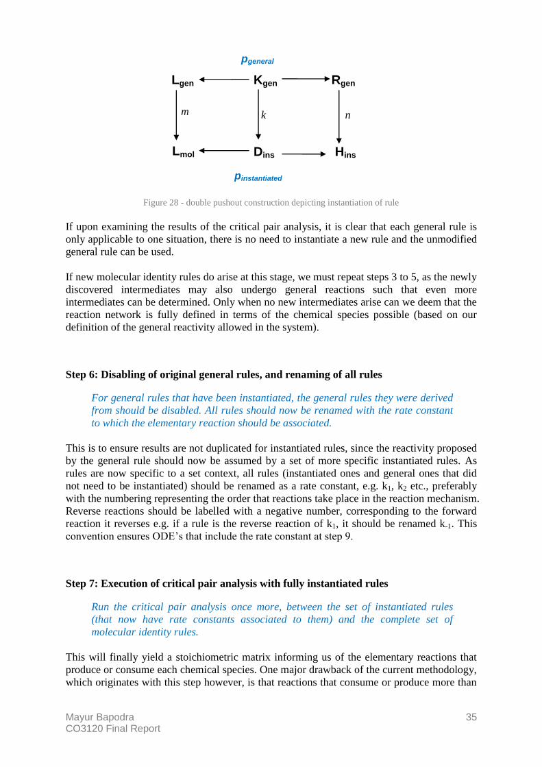
Mayur Bapodra 35 CO3120 Final Report
Figure 28 - double pushout construction depicting instantiation of rule
If upon examining the results of the critical pair analysis, it is clear that each general rule is
only applicable to one situation, there is no need to instantiate a new rule and the unmodified
general rule can be used.
If new molecular identity rules do arise at this stage, we must repeat steps 3 to 5, as the newly
discovered intermediates may also undergo general reactions such that even more
intermediates can be determined. Only when no new intermediates arise can we deem that the
reaction network is fully defined in terms of the chemical species possible (based on our
definition of the general reactivity allowed in the system).
Step 6: Disabling of original general rules, and renaming of all rules
For general rules that have been instantiated, the general rules they were derived
from should be disabled. All rules should now be renamed with the rate constant
to which the elementary reaction should be associated.
This is to ensure results are not duplicated for instantiated rules, since the reactivity proposed
by the general rule should now be assumed by a set of more specific instantiated rules. As
rules are now specific to a set context, all rules (instantiated ones and general ones that did
not need to be instantiated) should be renamed as a rate constant, e.g. k1, k2 etc., preferably
with the numbering representing the order that reactions take place in the reaction mechanism.
Reverse reactions should be labelled with a negative number, corresponding to the forward
reaction it reverses e.g. if a rule is the reverse reaction of k1, it should be renamed k-1. This
convention ensures ODE‟s that include the rate constant at step 9.
Step 7: Execution of critical pair analysis with fully instantiated rules
Run the critical pair analysis once more, between the set of instantiated rules
(that now have rate constants associated to them) and the complete set of
molecular identity rules.
This will finally yield a stoichiometric matrix informing us of the elementary reactions that
produce or consume each chemical species. One major drawback of the current methodology,
which originates with this step however, is that reactions that consume or produce more than
Kgen Lgen Rgen
Lmol Dins Hins
pgeneral
pinstantiated
m k n

Mayur Bapodra 36 CO3120 Final Report
one of a certain molecule cannot yet be ascertained. This is discussed in more detail in the
“Critical Appraisal” section. It is a flaw that should be solvable given more time.
If we view the resulting “.cpx” file in AGG, we are presented with a table that already closely
resembles the stoichiometric matrix that we need to derive ODE‟s. The following is the
conflicts analysis summary table for the SN1 reaction (after rule instantiation):
Figure 29 - AGG critical pair conflicts summary example
Only the upper right corner of the table is useful since the other rule pairings are not
necessary for kinetic analysis.
Step 8: Removal of structurally equivalent overlappings for instantiated rules
The critical overlappings obtained from Step 7 are passed through the Structural
Equivalence analysis program to remove spurious pairs so that only unique
overlappings remain.
The logic behind this step was presented in step 4. After performing this step, we are finally
presented with the stoichiometric matrix needed for the derivation of ODE‟s. The table in
figure 29 is reduced to that in figure 30.

Mayur Bapodra 37 CO3120 Final Report
Figure 30 - AGG critical pair conflicts summary example after structural equivalence reduction
Step 9: Execution of ODE extraction program
Run the ODE extraction program with the output “.cpx” file from Step 8 as input.
This will generate the ODE’s from the stoichiometric matrix and output them in
string format in a text file.
This stage uses the theory set out in “A Chemistry Background” of the “Relevant Background
Information” section. The output currently is in string format. However, the output can be
modified to any format necessary (e.g. XML). Integration with step 10 requires knowledge of
the specific math solver to be used and its input format. As step 10 was not fully realised in
the timescale of the project, it was decided that the output would simply be in string format,
to demonstrate that output is possible. Currently, it has the following format:
d[CH3+]/dt = -k-1[CH3+][Cl-] +k-2[CH3O+H2] +k1[CH3Cl] -k2[CH3+][H20]
d[CH3Cl]/dt = +k-1[CH3+][Cl-] -k1[CH3Cl]
There is one such line for each chemical species in the reaction network.
Step 10: Solving ODE’s using a 3rd
party math solver
Pass the ODE’s extracted in Step 9 into a suitable math solver software. A single
equation defining the progress of the reaction should be returned, in terms of the
change in concentration of one interesting species with time.
Although this step was not completed for the project, it is included for completion. In the
final stage, a 3rd
party math solver allows us to use the results of the kinetic analysis to
generate quantitative data and a graph representing the kinetic profile of the reaction. For this,
the values of all of the rate constants for the reaction need to be known. These can be derived
by numerous small experiments or gathered from existing sources. While these sources have

Mayur Bapodra 38 CO3120 Final Report
not been investigated, further research should reveal libraries (perhaps online) where such
information on reactions is maintained.
The results of this final stage can be used to validate our reaction mechanism. If the extracted
graph does not have the same form as established data for a particular reaction, it is clear that
the reaction rules were not complete or perhaps implemented incorrectly.

Mayur Bapodra 39 CO3120 Final Report
6. Implementation
The implementation of our methodology involved three distinct newly constructed
components. Each of these was implemented as a self-contained Java module and had the
following functions:
1. Critical pair analysis
2. Structural equivalence testing
3. ODE extraction
These were combined into a simple command line user interface (using shell and batch
scripting) which we shall call the kinetic analysis suite. This section will first cover how this
suite, along with AGG, can be used to apply our methodology to a concrete example,
specifically which steps in the methodology each tool/module relates to. A description of the
Java coding that was needed to implement each of the three modules is then given, along with
an account of the developed batch/shell script.
Tools that implement the methodology
Steps 1 and 2: AGG
To input rules, start graph and type graph AGG is used:
Figure 31 - main layout of AGG
List of components of grammar, i.e. start graphs, type graphs, rules,
constraints etc.
Left and right hand side of currently highlighted rule (also the area used to
define constraints)
Nodes and edge types defined for current
grammar
Area for defining start graph and type graph, and shows results of rule application

Mayur Bapodra 40 CO3120 Final Report
The red area can be used in step 2 to see which new chemical species occur as the result of
applying rules to previous graphs. Further documentation on the use of AGG can be found at
[19].
Steps 3 and 4: Kinetic Analysis Script
Here the prepared shell scripts need to be run. Initially the user is presented with an option of
whether they wish to run the full suite or component programs. For steps 2 and 3, the user
should choose “no”. Next, they are presented with an option for which program they wish to
run. For step 2, option 1 (“Critical Pair Analysis”) should be chosen. For step 3, when the
user has started the program for a second time, option 2 (“Structural Equivalence Analysis of
Pairs”) should be chosen. In both cases, they will be asked to input the location of the input
file.
Figure 32 - kinetic analysis program, steps 2 and 3
Step 5: AGG Critical Pair GUI
Critical pairs can be examined using AGG‟s critical pair GUI (figure 33). This is accessed
from the main AGG window by selecting “Analyzer > Critical Pair Analysis > Load > In
This Window” from the menu bar.
A summary table of the total conflicts and dependencies is given initially. By clicking a
square in this table the actually critical overlappings along with the 2 conflicting rules can be
examined for a rule pair. The top half of figure 33 shows the two conflicting rules. The graph
in the bottom right corner shows the critical overlapping. The nodes highlighted in green
show the graph objects that are responsible for the conflict. Mapping identities allow the user
to relate these to the same nodes and edges in the rules.
For this step, each critical overlapping should be examined to see if this rule needs to be
instantiated (i.e. more context introduced to the rule to make it more specific). If it does, the
main AGG window should be returned to, and the new rule added. The rule should then be
applied to the molecule for which the critical overlapping was found, and the new molecule
added as a new identity rule.

Mayur Bapodra 41 CO3120 Final Report
Figure 33 - critical pair analysis GUI module of AGG
Step 6: AGG
This step requires AGG once more. Once the rules have been instantiated, the old rules
should be disabled, by right clicking them in the grammar components list and selecting
“disabled”.
Steps 7, 8 and 9: Kinetic Analysis Script
The script should be run once more. This time, the full analysis suite option should be chosen.
Once the analysis is complete, the user is presented with the message in figure 34, which tells
them the filename which contains the generated ODE‟s. These are also printed to the system
output during the analysis.
Step 10: Third Party Algebra Solver
This part was not completed in time, partially due to the very simple nature of the case study
used, which did not require quantitative verification of results. Several commercial
applications were researched however. The majority of these were not freeware, especially
the most suitable for solving differential equations.

Mayur Bapodra 42 CO3120 Final Report
Figure 34 - result of running complete kinetic analysis suite
The AGG API
This API (for version 1.6.4) is included on the software CD for the project. Details of how to
access it are included on the readme file. AGG is an open source graph transformation tool
that is available at [19]. It is widely used to implement graph grammars and contains a depth
of functionality that can be accessed through its API, allowing low-level access to and the
opportunity to extend what is presented in its GUI. Because of the ease with which rules, type
graphs, and graphs can be implemented in AGG, it was a natural choice for the
implementation of the project. There are very few free open source graph transformation
tools like it. More information on its development and evolution can be found at [19].
In order to adapt what the software does to our needs, several classes needed to be extended,
and others were required for low-level functionality. At times, this proved extremely difficult.
The software itself has some depth and not all classes have complete Javadoc comments. This
is perfectly understandable for a non-commercial piece of software. Fortunately, the source
code was available which allowed us to deduce each method‟s purpose from its code and also
included some non-Javadoc comments. This was partially written in German, but use of
online translators helped translate parts of this. Nevertheless, the complexity of understanding
the API was a great technical challenge. With perseverance, and many hours of investigation,
however, much of the functionality required was attained. When it was felt that progress was
not being made at all (see the section on structural equivalence testing), help was available
directly from a member of the AGG development team.
The critical pair analysis part of AGG was the bottleneck in the methodology as it was
extremely memory intensive and time-consuming. Certain grammars actually had to be
abandoned (e.g. the esterification case study) because the Java virtual machine eventually ran
out of heap space. This is a limitation of the software that members of the AGG staff are
currently looking into. For future work, it would be extremely helpful if this problem was
resolved. In the meantime, alternative software that can carry out critical pair analysis for
graph transformation systems should be researched.

Mayur Bapodra 43 CO3120 Final Report
Critical Pair Analysis
The classes needed for this part are arranged in the following package structure:
agg.parser
MB294ComputeCriticalPairs
MB294DependencyPairContainer
extends DependencyPairContainer
MB294ExcludePairContainer
extends ExcludePairContainer
MB294ParserFactory
mb294
CPAnalysisSetup
Figure 35 - critical pair analysis package structure
As can be seen from this package structure, many of the classes are extensions of existing
AGG classes. MB294ComputeCriticalPairs is an almost exact copy of ComputeCriticalPairs,
with minor changes. This class could not be extended as certain methods that needed to be
overridden in the subclass required copying code from the superclass, and this contained
some private data members.
The main purpose of the modification to AGG‟s own critical pair analysis program is that this
conducts an analysis of critical pairs between every possible pairing of rules. Kinetic analysis
only requires the analysis of pairs where one member is a reaction rule and the other is a
molecular identity rule. CPAnalysisSetup loads and analyses a grammar, separating the rules
into two lists, one for reaction rules and the other for molecular identity rules. The crucial
code segment is given below:
Code 1 - CPAnalysisSetup, setUpRules method
This method extracts all of the enabled rules from its associated grammar as a list. Then using
a list iterator, checks each rule. If the LHS and RHS of the rule are identical, it is an identity
054 private void setUpRules() {
055 System.out.print("Sorting rules...");
056 long start = System.currentTimeMillis();
057 List<Rule> allRules = gragra.getListOfEnabledRules();
058 ListIterator<Rule> itr = allRules.listIterator();
059 while (itr.hasNext()) {
060 Rule tmp = itr.next();
061 if (tmp.getLeft().compareTo(tmp.getRight())) {
062 identityRules.add(tmp);
063 } else {
064 reactionRules.add(tmp);
065 }
066 }
067 long elapsedTimeMillis = System.currentTimeMillis() - start;
068 System.out.println("Finished sorting rules in " + elapsedTimeMillis
069 + " milliseconds");
070 }

Mayur Bapodra 44 CO3120 Final Report
rule and is added to this object‟s identity rules list data member, else it is assumed to be a
reaction rule and is added to this object‟s reaction rules list.
The scheduling of rule pairs for critical pair analysis takes place in AGG‟s
ExcludePairContainer class for conflicts. MB294ExcludePairContainer extends this class and
overrides the fillContainers method (responsible for scheduling pair analysis). Its constructor
creates a new CPAnalysisSetup object, passing in as a parameter the graph grammar for
which it is being used. MB294ExcludePairContainer then has two extra data members – a list
of identity rules and a list of reaction rules.
Code 2 - MB294ExcludePairContainer, fillContainers method
Some of this code is copied from the superclass‟ method. Lines 51-62 are the crucial part
which carries out the scheduling. For every reaction rule, every member of the identity rules
list is paired with it and scheduled for computing critical overlappings (line 59).
scheduleForComputing is a method of the superclass.
Similarly, for DependencyPairContainer, which computes sequentially dependent pairs,
MB294DependencyPairContainer extends this and overrides the following crucial method.
Code 3 - MB294DependencyPairContainer, computeCritical method
34 @Override
35 protected synchronized void computeCritical(Rule r1, Rule r2){
36 if (reactionRules.contains(r1) && identityRules.contains(r2)){
37 super.computeCritical(r1, r2);
38 }
39 else {
40 //do nothing
41 }
42 }
40 @Override
41 protected void fillContainers() {
42
43 if (useHostGraph && grammar != null) {
44 grammar.getApplicableRules(testGraph, strategy);
45 }
46
47 if (!useHostGraph) {
48 isComputed = false;
49 }
50
51 ListIterator<Rule> itr1 = reactionRules.listIterator();
52
53 while (itr1.hasNext()) {
54 Rule r1 = itr1.next();
55
56 ListIterator<Rule> itr2 = identityRules.listIterator();
57 while (itr2.hasNext()) {
58 Rule r2 = itr2.next();
59 this.scheduleForComputing(r1, r2);
60 }
61
62 }
63
64 if (!useHostGraph) {
65 isComputed = true;
66 }
67 }

Mayur Bapodra 45 CO3120 Final Report
In the original superclass, all rule pairs are automatically scheduled for computing. In order to
restrict the pairs that are actually computed, we override the computeCritical method and
check whether the rule 1 parameter is a reaction rule and rule 2 is an identity rule. If they are,
the superclass‟ original computeCritical method is called. Otherwise, the method does
nothing, thereby successfully bypassing the computation of unnecessary pairs.
In the original ComputeCriticalPairs class, the analysis engine retrieves and uses
ExcludePairContainer and DependencyPairContainer objects (used to calculate and store
critical pairs) from a ParserFactory object. MB294ParserFactory is a copy of this class, which
instead returns MB294ExcludePairContainer and MB294DependencyPairContainer objects
(see lines 37, 47 and 51 of the source code). MB294ComputeCriticalPairs then simply
retrieves the new customised PairContainer objects using MB294ParserFactory wherever
ParserFactory was originally used, as in the following code segement:
Code 4 - MB294ComputeCriticalPairs, use of MB294ParserFactory
This ensures that this program only calculates the pairs needed, and is a first attempt at a
more efficient and optimized analysis.
Structural Equivalence Testing
To reduce structurally equivalent overlappings (in terms of Chemistry) a program was
developed that could accept the “.cpx” XML file output from the critical pair analysis,
perform the reduction, and save the new pairs in a new file (with the suffix
“_structuremod.cpx”). The package structure for this program is as follows:
mb294
StructuralEquivalenceAnalysis
Code 5 - structural equivalence testing package structure
The source code for this class is heavily commented so only a summary of our method is
presented here. The constructor uses API methods to load critical pair information from a file
(identified by filename supplied through the command line). The method
reduceStructurallyEquivalentOverlappings then extracts all the overlapping information and
performs the reduction. For each rule pair, all overlappings are tested for uniqueness. It was
decided that the best way to do this would be to apply the reaction rule to the molecular graph
represented by the LHS of the identity rule, using the match provided by the critical
overlapping of the two rules. The result of the application should be checked for isomorphism
:
:
357 if (excludePairContainer == null)
358 excludePairContainer = MB294ParserFactory
359 .createEmptyCriticalPairs(gragra,
360 CriticalPairOption.EXCLUDEONLY, cpOption
361 .layeredEnabled());
362
:
:

Mayur Bapodra 46 CO3120 Final Report
with all other unique overlappings for this rule pair. If it is isomorphic to any of them, it
should be discarded, else it should be added as a unique overlapping. Applying the rule is a
sufficient check for structural uniqueness.
The help of Olga Runge (an AGG developer) should be greatly acknowledged here. Although
the method presented above was recognised as the best way to test for structural uniqueness,
a way to apply the rule using the match information from the critical pair could not be
deduced from the API without affecting the original XML file. A method was designed, but it
led to nodes and edges in the critical overlapping being deleted when written back to file.
Also, the method of reversing a rule and applying it (necessary for checking for uniqueness in
dependency pair overlappings, see the construction in figure 14) could not be deduced. Olga
Runge‟s help and advice at this stage through numerous emails was invaluable and very
greatly appreciated. Code that she helped with is noted in comments within the source code.
The makeStep method in its entirety was provided by Olga.
ODE Extraction
The classes needed for this part are arranged in the following package structure:
mb294
ODEArray
ODEExtraction
RateLawArray
StoichiometricMatrix
Code 6 - ODE extraction package structure
ODEExtraction is the program with a main method that produces the ODE‟s. It has an object
of each of the other 3 classes listed above as data members. All of these classes are heavily
commented so only a summary of their main functions are presented here.
ODEArray contains a Hashtable that stores these ODE‟s. For each identity rule key in the
Hashtable (i.e. chemical species), there is a string representation of its corresponding ODE as
the object. StoichiometricMatrix takes the overlappings data from the XML output file of the
structural equivalence component and discards superfluous information making it easier for
other methods to process. The stoichiometric matrix data is stored as a Hashtable, with
reaction rules as keys, and another Hashtable as objects. This second Hashtable has the
identity rules as keys and Integers as objects. These integers represent the entry in the
stoichiometric matrix for each reaction-identity rule pairing. The RateLawArray object is
created using information from a StoichiometricMatrix object (as described in “Relevant
Background Information”). The rate laws for each elementary reaction are stored as an array
of pairs. Each pair in the array consists of a reaction rule, and a string representing its rate law.
ODEExtraction loads overlappings data in the same way that the structural equivalence
module does, using API methods. Once loaded, this class instantiates an
ExcludePairContainer and a DependencyPairContainer object to store conflict and
dependency overlapping information respectively. This occurs in the constructor. The main
method calls this constructor and then calls the following method:

Mayur Bapodra 47 CO3120 Final Report
Code 7 - ODEExtraction, outputODEs method
The first task is population of the StoichiometricMatrix object (line 102). The method that
does the work within the private populateStroichiometricMatrix method is the fillMatrix
method of StoichiometricMatrix, which takes the no. of critical conflict overlappings for each
reaction-identity rule pair (the no. of molecules consumed by a reaction) and minuses it from
the no. of dependency overlappings for the same pair (the no. of molecules produced by the
reaction). This gives the overall effect a reaction has on a particular chemical species. This
number is added to the stoichiometric matrix for this reaction-identity rule pair.
When the stoichiometric matrix is filled, the rate law array is extracted from it (line 104).
This is done by the fillArray method in the RateLawArray class. For each elementary
reaction, we look for negative entries in the stoichiometric matrix. By assuming that negative
entries mean involvement in initiation of a reaction, we can extract the rate law for that
reaction.
generateODEs (line 106) then calls the generateODEArray method of ODEArray. This
simulates the matrix multiplication of the rate law array by the stoichiometric matrix and
stores the results. This class also contains a method that returns all the ODE‟s as a String
object. Lines 108 to 118 in code 7 show how the ODE‟s are output to console and to a text
file using this String.
Running the Kinetic Analysis
The classes described above were all compressed into a JAR file entitled
“kinetic_analysis_in_agg.jar” and placed in the agg root directory, where the JAR files that
hold AGG‟s other classes are also located. A batch file (for Windows) and a shell script (for
Linux) were created labelled “kinetics.bat” and “kinetics.sh” respectively. These scripts are
the GUI through which many steps in the methodology can be performed, guiding the user
through input and output of the 3 programs described above. There are some variables which
must be changed in these files to allow them to run on a specific machine (such as
JAVA_HOME). A “maxheap” variable also specifies the maximum heap memory allowed by
the Java virtual machine. As mentioned previously, the critical pair analysis is extremely
memory intensive and can fail if not supplied with enough heap space. This variable should
be set as large as possible. An additional argument is supplied to the Java virtual machine,
100 public void outputODEs() throws Exception {
101 System.out.println("\n");
102 populateStoichiometricMatrix();
103 getStoichiometricMatrix().printStoichiometricMatrixInfo();
104 populateRateLawMatrixFromStoichiometricMatrix();
105 getRateLawArray().printRateLawArray();
106 generateODEs();
107
108 String output = getODEArray().odeEquationsToString();
109 System.out.println("\n\nPRINTING ODEs:\n" + output + "\n");
110 System.out.println("Writing ODEs to text file with name " + newfilename
111 + " ...");
112 // write the ODEs string to file
113 BufferedWriter out = new BufferedWriter(new FileWriter(newfilename));
114 out.write(output);
115 out.flush();
116 out.close();
117 // System.out.println("Done.");
118 }

Mayur Bapodra 48 CO3120 Final Report
namely “XX:-UseGCOverheadLimit”. This ensures that OutOfMemory errors are not thrown
if the virtual machine spends too much time in garbage collection. This was necessary for
larger grammars which led to many such errors. However, Sun Microsystems deem this an
unstable option, and it should possibly be removed in future iterations when AGG‟s critical
pair analysis engine is improved for efficiency (see
http://java.sun.com/javase/technologies/hotspot/vmoptions.jsp for more details).
The scripts enable the user to run all three programs described above to run consecutively
without any need for user interaction. In order to prevent subsequent programs from running
when an exception occurs in an earlier program, system exit codes were utilised. For the
structural equivalence analysis and ODE extraction, if an exception occurred, the main
method returns a -1 exit code, else 10 is returned (highlighted in red):
Code 8 - StructuralEquivalenceAnalysis, main method demonstrating use of exit codes
This is not possible for the main method of MB294CriticalPairAnalysis however.
Code 9 - MB294CriticalPairAnalysis, main method
Line 416 initiates a thread. While this thread is running the main method continues to execute
its next line in its own thread of execution. Any system exit code would immediately cause
this program to end. Therefore, for this program, we use the default system exit code (of
value 0) which is automatically returned when all threads are finished. In the event of an
exception however, -1 can still be returned.
The Windows script uses these codes as shown in code 10. If an error is returned the control
is forwarded to the printing out of an error message and then the end of the script. Otherwise,
the next program is started with the output file of the last program as input.
413 public static void main(String[] args) {
414 try {
415 MB294ComputeCriticalPairs mcp = new MB294ComputeCriticalPairs();
416 mcp.run(args);
417 }catch (Exception e){
418 System.err.println("An error occurred during critical pair analysis!");
419 e.printStackTrace();
420 System.exit(-1);
421 }
422 }
379 public static void main(String[] args) {
380
381 try {
382 StructuralEquivalenceAnalysis sea = new StructuralEquivalenceAnalysis(
383 args[0]);
384 sea.processFileForStructuralEquivalence();
385 System.exit(10);
386 } catch (ArrayIndexOutOfBoundsException e) {
387 System.err
388 .println("There was an error loading your specified file - please try
again!");
389 e.printStackTrace();
390 System.exit(-1);
391 }
392
393 }// end of main method

Mayur Bapodra 49 CO3120 Final Report
Code 10 - Windows batch script demonstrating use of Java system exit codes
:section1command
java -Xmx%MAXHEAP%m -XX:-UseGCOverheadLimit agg.parser.MB294ComputeCriticalPairs %file%
IF ERRORLEVEL 0 goto :section1-1
IF ERRORLEVEL -1 goto :section1-1error
:section1-1
set nextfile=%file:.ggx=_out.cpx%
java -Xmx1000m mb294.StructuralEquivalenceAnalysis %nextfile%
IF ERRORLEVEL 1000 (goto :section1-2) ELSE (goto :section1-2error)
:section1-2
set lastfile=%nextfile:_out.cpx=_out_structuremod.cpx%
java -Xmx1000m mb294.ODEExtraction %lastfile%
IF ERRORLEVEL 1000 (goto :section1complete) ELSE (goto :section1-3error)
:
:
:
:section1-1error
echo There was a problem running the critical pair analysis.
goto :eof
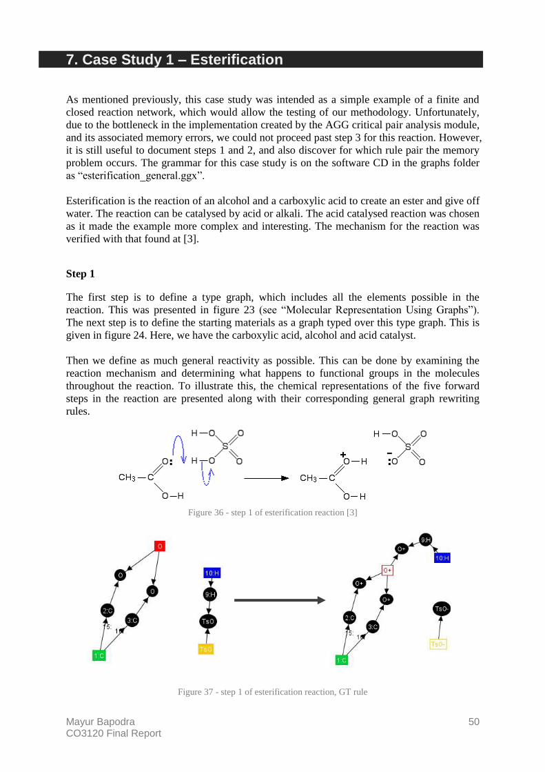
Mayur Bapodra 50 CO3120 Final Report
7. Case Study 1 – Esterification
As mentioned previously, this case study was intended as a simple example of a finite and
closed reaction network, which would allow the testing of our methodology. Unfortunately,
due to the bottleneck in the implementation created by the AGG critical pair analysis module,
and its associated memory errors, we could not proceed past step 3 for this reaction. However,
it is still useful to document steps 1 and 2, and also discover for which rule pair the memory
problem occurs. The grammar for this case study is on the software CD in the graphs folder
as “esterification_general.ggx”.
Esterification is the reaction of an alcohol and a carboxylic acid to create an ester and give off
water. The reaction can be catalysed by acid or alkali. The acid catalysed reaction was chosen
as it made the example more complex and interesting. The mechanism for the reaction was
verified with that found at [3].
Step 1
The first step is to define a type graph, which includes all the elements possible in the
reaction. This was presented in figure 23 (see “Molecular Representation Using Graphs”).
The next step is to define the starting materials as a graph typed over this type graph. This is
given in figure 24. Here, we have the carboxylic acid, alcohol and acid catalyst.
Then we define as much general reactivity as possible. This can be done by examining the
reaction mechanism and determining what happens to functional groups in the molecules
throughout the reaction. To illustrate this, the chemical representations of the five forward
steps in the reaction are presented along with their corresponding general graph rewriting
rules.
Figure 36 - step 1 of esterification reaction [3]
Figure 37 - step 1 of esterification reaction, GT rule

Mayur Bapodra 51 CO3120 Final Report
As can be seen in figure 37, the whole molecule is not presented in the rule, only the part that
undergoes reaction. This makes the rule applicable to any molecule that might have this
functional group, which is exactly what is required. This reaction is reversible, so the C=O
double bond can be deprotonated once it is protonated. This is represented in the grammar by
a rule labelled step-1, where the LHS and RHS of step1 are simply switched.
Figure 38 - step 2 of esterification reaction [3]
Figure 39 - step 2 of esterification reaction, GT rule
Step 2 of the reaction is the attack of the negatively charged oxygen in the alcohol on the now
positively charged (due to the protonation in step 1) central carbon atom in the carboxylic
acid. This results in the joining of the two large molecules into one. This step is also
reversible and is represented by step-2 in the grammar.
Figure 40 - step 3 of esterification reaction [3]
Figure 41 - step 3 of esterification reaction, GT rule

Mayur Bapodra 52 CO3120 Final Report
This reaction is the simple change in the location of a proton (H atom) within the newly
formed large molecule. The reverse of this reaction is labelled step-3 in the grammar.
Figure 42 - step 4 of esterification reaction [3]
Figure 43 - step 4 of esterification reaction, GT rule
Here, the protonated OH group leaves the larger molecule as water, allowing the C=O double
bond to reform. The reverse of this step is labelled step-4. The representation of the positively
charged C=O+ in the RHS of the graph transformation rule is identical to that presented in
figure 42. Here, the electrons in the O-C=O+ structure are delocalised over all 3 bonds, and
the positive charge can also be spread over all three atoms.
Figure 44 - step 5 of esterification reaction [3]
The final step in the reaction (also reversible) is deprotonation of the reformed C=O double
bond. However, this was not added as a general rule, as this reactivity is already captured by
step-1. Step 5 and 6 of the methodology would see two instantiations of the step-1 reaction
rule, one for the initial deprotonation (as a reverse of step1) and one for the final
deprotonation. Each would be assigned their own rate constant.
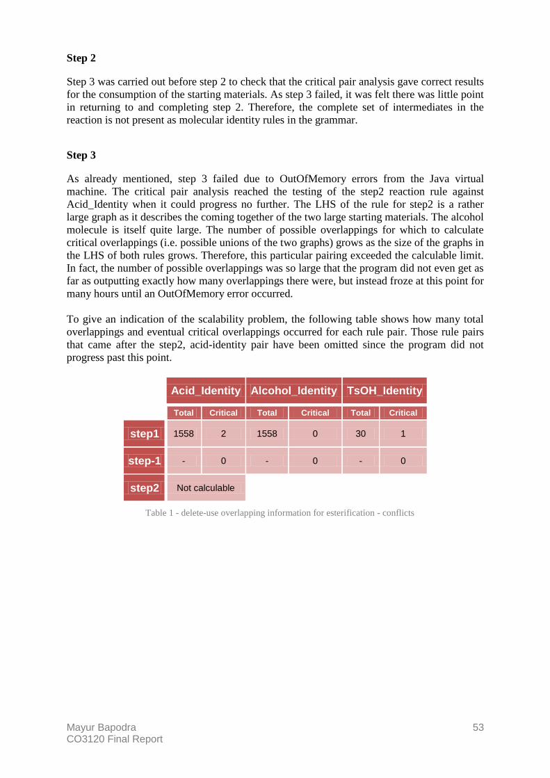
Mayur Bapodra 53 CO3120 Final Report
Step 2
Step 3 was carried out before step 2 to check that the critical pair analysis gave correct results
for the consumption of the starting materials. As step 3 failed, it was felt there was little point
in returning to and completing step 2. Therefore, the complete set of intermediates in the
reaction is not present as molecular identity rules in the grammar.
Step 3
As already mentioned, step 3 failed due to OutOfMemory errors from the Java virtual
machine. The critical pair analysis reached the testing of the step2 reaction rule against
Acid_Identity when it could progress no further. The LHS of the rule for step2 is a rather
large graph as it describes the coming together of the two large starting materials. The alcohol
molecule is itself quite large. The number of possible overlappings for which to calculate
critical overlappings (i.e. possible unions of the two graphs) grows as the size of the graphs in
the LHS of both rules grows. Therefore, this particular pairing exceeded the calculable limit.
In fact, the number of possible overlappings was so large that the program did not even get as
far as outputting exactly how many overlappings there were, but instead froze at this point for
many hours until an OutOfMemory error occurred.
To give an indication of the scalability problem, the following table shows how many total
overlappings and eventual critical overlappings occurred for each rule pair. Those rule pairs
that came after the step2, acid-identity pair have been omitted since the program did not
progress past this point.
Acid_Identity Alcohol_Identity TsOH_Identity
Total Critical Total Critical Total Critical
step1 1558 2 1558 0 30 1
step-1 - 0 - 0 - 0
step2 Not calculable
Table 1 - delete-use overlapping information for esterification - conflicts

Mayur Bapodra 54 CO3120 Final Report
8. Case Study 2 – SN1 Reaction
SN1 stands for unimolecular nucleophilic substitution. It involves the replacement of a good
leaving group on a carbon atom (e.g. a chlorine atom) with a group that is less able to support
negative charge (e.g. a hydroxyl, OH, group). Unimolecular refers to the fact that the rate
determining step involves only one molecule, the halocarbon. The reaction occurs once the
Cl- group leaves the molecule. There is also an SN2 reaction which is bimolecular in its rate
determining step. The substituting group and the halocarbon must collide for reaction to
occur. A transition state where the new group and leaving group are both partially bonded to
the central carbon atom occurs, before the leaving group leaves. There is one less step in the
SN2 reaction, so SN1 was chosen to make the example more testing of the methodology.
This reaction is very simple and its selection was prompted by the memory problems that
occurred in the esterification example. The reactant molecules are quite small, so the number
of possible overlappings for each reaction rule during critical pair analysis is reduced. Despite
this, the analysis still took up to 80 minutes on some occasions for the instantiated grammar
using 2.6GB of heap memory on a Linux machine.
The general grammar can be found in the graphs folder of the software CD as
“SN1_general.ggx”. The instantiated grammar has filename “SN1_instantiated.ggx”.
Step 1
The type graph for this reaction is given below:
Figure 45 - SN1 type graph
The individual connections between different types of bond nodes present in the esterification
type graph are replaced with an inheritance relationship. To ensure every bond node is only
connected to one other bond node, the supertype BondNode has a 1 to 1 relation to itself. It is
now much easier to solve the problem described in “Molecular Representation Using Graphs”
where numerous constraints were needed to restrict multiple bond node connections. These
numerous constraints can be replaced by just one atomic constraint which must always be
false:

Mayur Bapodra 55 CO3120 Final Report
Atomic proposition: Atomic conclusion:
(empty)
Figure 46 - constraint limiting number of bonds allowed
However, as the connections between each type of bond node are no longer explicit, this type
graph has lost bond direction conventions. For example, there is no indication that if a C bond
node is connected to an O bond node, the edge should go from the C to the O. To solve this,
additional bond direction atomic constraints are added to the grammar. For the C-O example,
we have the following atomic constraint, which is developed into a graph constraint where
this atomic constraint is designated as always being false:
Atomic proposition: Atomic conclusion:
(empty)
Figure 47 - constraint designating direction of edges in bonds
In this type graph, O+ and C
+ no longer have their own bonding nodes. This was an
experiment to determine whether limiting the types of nodes made the grammar any more
efficient. Unfortunately, the results were inconclusive, as each time the grammar was run, the
time taken fluctuated greatly without any pattern. Nevertheless, the simpler type graph was
kept. This does however necessitate two further constraints that prevent both a C and C+
connecting to a single C bond node (and similarly for O and O+). The atomic constraint is
given below, and again this is developed into a graph constraint where it must always be
false:
Atomic proposition: Atomic conclusion:
(empty)
Figure 48 - constraint limiting C and C+ connection to same bond node
The starting materials are defined as follows:
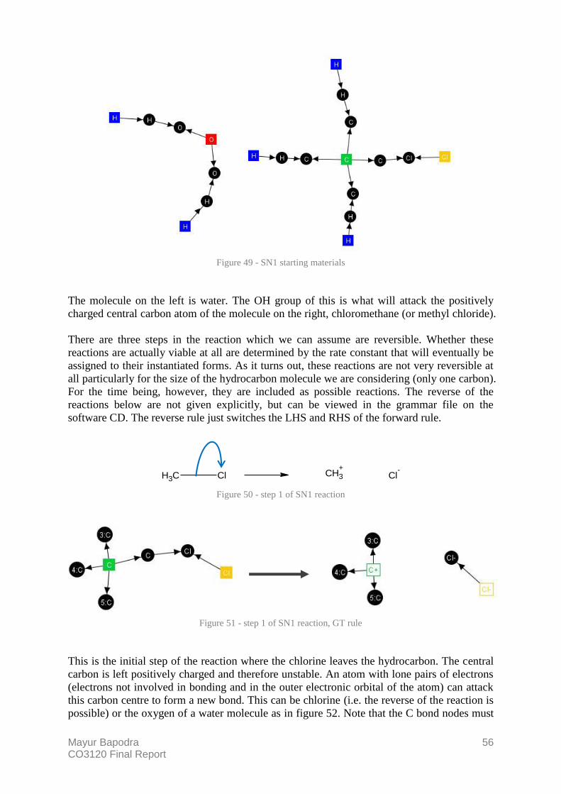
Mayur Bapodra 56 CO3120 Final Report
Figure 49 - SN1 starting materials
The molecule on the left is water. The OH group of this is what will attack the positively
charged central carbon atom of the molecule on the right, chloromethane (or methyl chloride).
There are three steps in the reaction which we can assume are reversible. Whether these
reactions are actually viable at all are determined by the rate constant that will eventually be
assigned to their instantiated forms. As it turns out, these reactions are not very reversible at
all particularly for the size of the hydrocarbon molecule we are considering (only one carbon).
For the time being, however, they are included as possible reactions. The reverse of the
reactions below are not given explicitly, but can be viewed in the grammar file on the
software CD. The reverse rule just switches the LHS and RHS of the forward rule.
CH3 Cl CH3
+Cl
-
Figure 50 - step 1 of SN1 reaction
Figure 51 - step 1 of SN1 reaction, GT rule
This is the initial step of the reaction where the chlorine leaves the hydrocarbon. The central
carbon is left positively charged and therefore unstable. An atom with lone pairs of electrons
(electrons not involved in bonding and in the outer electronic orbital of the atom) can attack
this carbon centre to form a new bond. This can be chlorine (i.e. the reverse of the reaction is
possible) or the oxygen of a water molecule as in figure 52. Note that the C bond nodes must

Mayur Bapodra 57 CO3120 Final Report
be included in the definition of the general rule in figure 51. This is because the central C
atom changes to a C+
atom. This is a deletion of the C followed by creation of the C+. During
the deletion, if the C bond nodes are not explicitly shown in the rule, a violation of the
dangling rule occurs (see “Molecular Representation Using Graphs”).
O
H
H
C+
H
H
H
CO+
H
H
HH
H
Figure 52 - step 2 of SN1 reaction
Figure 53 - step 2 of SN1 reaction, GT rule
The final step of the reaction is deprotonation of the positively charged O to leave the alcohol
(methanol in this case). The Cl- generated from step 1 co-ordinates with the H
+ that is
released, to give hydrochloric acid (HCl).
CO+
H
H
HH
H
Cl-
CO
H
H
H
H
ClH
Figure 54 - step 3 of SN1 reaction
Figure 55 - step 3 of SN1 reaction, GT rule

Mayur Bapodra 58 CO3120 Final Report
Step 2
Applying the rules to the start graph non-deterministically yielded the following preliminary
intermediates and products. Each one was added as a molecular identity rule. The molecules
in the start graph (CH3Cl and H2O in figure 49) were also added as identity rules.
Chemical Formula
Structural Formula Graph Representation
CH3Cl C Cl
H
H
H
H2O OHH
CH3+
C+
H
H
H

Mayur Bapodra 59 CO3120 Final Report
Cl- Cl-
CH3O+H2 CO
+
H
H
HH
H
HCl Cl H
CH3OH O
H
H
HH
Table 2 - preliminary intermediates in SN1 reaction
Step 3
The AGG screenshot below shows the exact results obtained from the first pass critical pair
analysis.

Mayur Bapodra 60 CO3120 Final Report
Table 3 - summary of conflict overlappings from critical pair analysis (first pass)
Table 4 - summary of dependency overlappings from critical pair analysis (first pass)
To give an indication of the scalability of the critical pair analysis, the following tables show
how many total overlappings and eventual critical overlappings occurred for each rule pair at
this stage (as shown for the esterification example).
As can be seen from this, a total of over 32,500 inclusions need to be checked for certain rule
pairs. These correspond to the combination of the reaction rules consisting of most nodes in
the LHS graph, and identity rules describing the largest molecules, namely step2 and
CH3O+H2. Adding even one more node to the LHS of the rule takes the no. of overlappings
to check to over 100,000. This is a serious limitation of the AGG tool to handle more
complex molecular structures and reactions, particularly if a reaction rule requires slightly
more local context than that represented in the reaction rules of this case study.

Mayur Bapodra 61 CO3120 Final Report
CH3Cl H20 CH3+ Cl- CH3O+H2 CH3OH HCl
Total Critical Total Critical Total Critical Total Critical Total Critical Total Critical Total Critical
step1 663 6 - 0 8 0 - 0 89 0 89 0 4 0
step-1 - 0 - 0 27 6 4 1 - 0 - 0 - 0
step2 - 0 63 2 135 6 - 0 - 0 - 0 504 1
step-2 445 0 26 0 40 0 - 0 32593 12 6448 0 - 0
step3 - 0 32 0 - 0 4 1 1531 2 208 0 - 0
step-3 100 0 45 0 - 0 - 0 - 0 315 1 29 1
Table 5 - delete-use overlapping information for SN1 - conflicts
CH3Cl H20 CH3+ Cl- CH3O+H2 CH3OH HCl
Total Critical Total Critical Total Critical Total Critical Total Critical Total Critical Total Critical
step1 - 0 - 0 27 6 4 1 - 0 - 0 - 0
step-1 663 6 - 0 8 0 - 0 89 0 89 0 4 0
step2 445 0 26 0 40 0 - 0 32593 12 6448 0 - 0
step-2 - 0 63 2 135 6 - 0 - 0 504 1 - 0
step3 100 0 - 0 - 0 - 0 - 0 315 1 29 1
step-3 - 0 32 0 - 0 4 1 1531 2 208 0 - 0
Table 6 - delete-use overlapping information for SN1 - dependencies
Step 4
Step 4 (structural equivalence testing of results of step 3) was bypassed for this case study as
the overlappings were quite easy to study without doing this step. For more complex
mechanisms though with larger molecules (and hence more critical overlappings with the
same structure) or more rules, this step would make manual analysis in step 5 far easier.
Step 5
Examination of the results from step 3 yields a necessary instantiation of the general rule,
step2. Step2 consumes H2O and CH3+ (deduced from the conflicts table), but also seems to
consume CH3OH. This suggests that the following reaction is also possible:

Mayur Bapodra 62 CO3120 Final Report
C+
H
H
H
C OH
H
H
H CH3
O+
CH3
H
Figure 56 - reaction of CH3OH with CH3+
In other words, the alcohol product, as well as water, can react with the carbocation. In fact,
this may even be a stronger reaction, as the CH3 group attached to the oxygen is very slightly
electron donating, meaning the push of the lone pair to the carbocation is made easier. This
intermediate would have been discovered at stage 2 of the methodology had the product
alcohol molecule been added to the start graph as a possible reactant.
The general rule, step2, therefore needs to be instantiated twice; once for the reaction with
water and once for the reaction with methanol. These new rules are shown in figures 57 and
58.
Figure 57 - instantiation of step2 for reaction with water
Figure 58 - instantiation of step2 for reaction with methanol
Notice that it is sufficient to replace one of the hydrogen atoms in the attacking molecule in
figure 57 with a single carbon. This introduces enough local context to make this rule apply
only to the product methanol, and not water. This is preferable to adding the entire molecule
as this increases the time taken for critical pair analysis, because more nodes equates to more
overlappings to check through. The reverse rules were also instantiated here.

Mayur Bapodra 63 CO3120 Final Report
At this stage, the new intermediates and instantiated rules were added to the grammar. With
the general rules still in place (in case they are applicable to the new intermediates) a second
critical pair analysis pass was tried. This led to OutOfMemory problems however. It seemed
that the new large molecule created by the reaction in figure 56 passed the threshold for
allowed analysis. As this was quite late in the project, a decision was made to ignore the
possibility that this reaction occurs, disabling the instantiated rule that represents it, and any
molecular identity rules of intermediates that arise from it. The verification of overall results
and extracted ODE‟s would take this omission into account.
After doing this, the critical pair analysis was reattempted. Once again an OutOfMemory
error occurred which prevented the analysis from completing. This was now due to the
instantiated rule set up for water (figure 57). It seemed that even two nodes and one edge
more than the number present in the general rule is enough to prevent the analysis engine
from completing successfully. Another strategy was needed that would use the general rule as
the instantiated rule for water then, but disallow the reaction with methanol. A negative
application condition (NAC) was employed to achieve this. NAC‟s are preconditions to rules.
They constitute a graph which if it occurs in the match for the LHS of the rule, prevents the
application of the rule for that match. The following NAC was added to the general rule for
step 2 (rule shown in figure 53).
Figure 59 - NAC for step2 general rule to create instantiated rule
The NAC specifies that a carbon bond node must not be connected to the oxygen bond node
with mapping identity 7, therefore disallowing the reaction of methanol with the carbocation.
Water is still able to react.
This simpler grammar that ignores the full reactivity of the system can be found on the
software CD in the graphs folder, with name “SN1_instantiated_simpler.ggx”. This grammar
was used for all subsequent steps in the methodology.
Step 6
Once the rules are instantiated and no further intermediates are found the general rules are
usually disabled. In our case, the instantiated rules which allowed the reaction with methanol
had to be disabled. In the end, the original general rules were used (one with an added NAC).
All reaction rules were renamed as rate constants. The “step” prefix in the name of every
general rule was replaced with a “k”. Hence, step1 became k1 and step-1 became k-1 etc.
Step 7
The critical pair analysis was run once again, yielding the following results:

Mayur Bapodra 64 CO3120 Final Report
Table 7 - summary of conflict overlappings from critical pair analysis (final pass)
Table 8 - summary of dependency overlappings from critical pair analysis (final pass)
As can be seen from table 4, the reaction of step2 (now k2) no longer consumes the methanol
product (CH3OH). These results are found in the file “SN1_instantiated_simpler_out.cpx” in
the results folder on the software CD.
Step 8
Running the structural equivalence analysis reduced the number of critical overlappings in
tables 4 and 5 to those in tables 6 and 7. All of the entries were reduced to 1, indicating that
all of the original overlappings were the same. This was verified to be the case by manually
examining the overlapping information produced in step 7.
These results are found in the file “SN1_instantiated_simpler_out_structuremod.cpx” in the
results folder on the software CD.

Mayur Bapodra 65 CO3120 Final Report
Table 9 - summary of conflict overlappings after structural equivalence analysis
Table 10 - - summary of dependency overlappings after structural equivalence analysis
Step 9
Finally, running the ODE extraction program yields the following ODE‟s:
d[CH3+]/dt = -k-1[CH3+][Cl-] +k-2[CH3O+H2] +k1[CH3Cl] -k2[CH3+][H20]
d[CH3Cl]/dt = +k-1[CH3+][Cl-] -k1[CH3Cl]
d[CH3O+H2]/dt = -k-2[CH3O+H2] +k-3[CH3OH][HCl] +k2[CH3+][H20] -k3[CH3O+H2][Cl-]
d[CH3OH]/dt = -k-3[CH3OH][HCl] +k3[CH3O+H2][Cl-]
d[Cl-]/dt = -k-1[CH3+][Cl-] +k-3[CH3OH][HCl] +k1[CH3Cl] -k3[CH3O+H2][Cl-]
d[H20]/dt = +k-2[CH3O+H2] -k2[CH3+][H20]
d[HCl]/dt = -k-3[CH3OH][HCl] +k3[CH3O+H2][Cl-]

Mayur Bapodra 66 CO3120 Final Report
Brief Analysis of results
The ODE‟s derived in step 9 do in fact agree with the ODE‟s derived by hand for the SN1
reaction, taking into account the omission of certain reactivity at steps 5 and 6. This is a
positive result that shows the methodology (and its implementation) are capable of deriving
ODE‟s for simple reactions. While the wider applicability of this methodology is limited (as
discussed earlier in “Methodology”), this is a substantial first step in developing a more
universally applicable method.
The SN1 reaction in reality is a very simple one and is often quoted as having a rate of:
][][
3
3 ClCHkdt
ClCHd
This is because the reaction k1 in our grammar, the departure of the Cl- group from CH3Cl, is
considered to be the rate determining step i.e. the only step of any significance to the rate.
Subsequent reactions occur very quickly once this step occurs. The equation above can
actually be derived from our ODE‟s from step 9. If all other elementary reactions do not
occur at all or are assumed to be very rare (particularly the reverse ones) k1 is the only rate
constant that doesn‟t have negligible value. For reactions that occur extremely quickly once
the rate determining step does, intermediates are immediately consumed so their
concentration throughout the reaction can be approximated to zero. If these approximations
are taken into account, the differential reaction for the rate of change of concentration of
CH3Cl approximates to the equation given above. Once concrete rate constants are found, any
arbitrary system of reactions will be reduced down in this way so that only significant
reactions remain. Our methodology ensures all possible reactivity is taken into account before
this simplification occurs.

Mayur Bapodra 67 CO3120 Final Report
9. Planning and Timescales
Tasks
The following is a preliminary account of the expected tasks of the project, as presented in
the Project Plan document. As predicted, these underwent significant changes as the project
progressed, new understanding came to light and new problems or challenges occurred. Due
to the open nature of the project, it would have been unwise to continually update and modify
the plan. This would have been time-consuming. It was discovered that any attempt to adhere
to a concrete plan limited further exploration in a particular area of interest and failed to
incorporate significant changes to the direction of the project. Therefore, the plan is presented
here unaltered, and a discussion of the deviations that occurred follow it.
1. Further background research
1.1 Stochastic graph transformation theory
This is fundamental to the project and therefore must be understood
clearly. In addition to what has already been read, other sources will be
investigated. Papers [10] and [11] will be thoroughly revised to ensure
complete familiarity with the process of creating stochastic graph
transformation systems.
1.2 Example stochastic graph transformation system
To ensure understanding, a simple example will be constructed in AGG,
with supporting tools for stochastic simulation. The major challenge here
may be tool support, as PRISM and GROOVE have not been
encountered yet. However, this stage will also allow us to gain
familiarity with these tools and AGG.
1.3 Research into CCS and π-calculus
In order to understand and learn from the methodology in [2], a quick
study of [15] will be undertaken. Some lecture notes from the
department‟s course on Communicating and Concurrent processes will
also be reviewed. [15] covers an extensive and technically involved
subject. The challenge here will be not to dwell on an area of computer
science that won‟t be used extensively in the final project. It will be
important to restrict the time given to this task.
2. Developing a Methodology
2.2 Deriving ordinary differential equations
This is the most important and possibly time-consuming part of the
project, and has been scheduled accordingly. This part will involve
formulating the methodology behind defining a stochastic graph

Mayur Bapodra 68 CO3120 Final Report
transformation from reactant molecules and how to assign rates to
transitions between graphs. This part of the project cannot be broken
down any further at this stage because of its theoretical nature – the
particular details of how the derivation will occur are not known at this
time. This stage will draw from all of the research conducted in part 1 of
the project, as well as additional chemistry research needed at this stage,
such as kinetics, thermodynamics, reaction mechanisms, and molecular
orbital theories. As already mentioned this is a highly theoretical and
challenging part of the project. There is substantial risk here if a suitably
accurate methodology cannot be formed. In this case, an iterative process
of simpler models (incorporating less and less real chemistry) will be
adopted in order to get some kind of methodology. Additionally, the
level of automation in the process of assigning rates can be lowered if
necessary. If finding the rates by checking the change in the molecular
orbital makeup of a molecule presents itself as too difficult and time-
consuming, the rate constant assignment can be reverted to a manual
process. Simplifying our case study subjects may also be an option if the
eventual methodology is deemed unsuitable for the existing ones.
Technical help will be requested from members of the Chemistry
department and from Prof. Heckel and Dr. Fer-Jan de Vries if necessary.
3. Tool Investigation
3.1 Tool investigation
AGG cannot be used for stochastic simulation despite being extremely
good for testing the application of transformation rules. At this stage
other tools such as PRISM, GROOVE and FERN should be investigated
to see how they can aid the project. Although these tools have not been
used before, [6], [10] and [11] outline their use in stochastic simulation.
Prof. Heckel has used [10] and [11] before and may be able to help at
this stage in case of difficulties.
3.2 Tool development
This step may not be necessary if existing tools are readily available.
However, if work needs to be done to develop a stochastic simulation
tool or integration with AGG, some time will be reserved for this. AGG
is implemented in Java and is supplied with an API for just such an
integration task. FERN may prove to be an ideal candidate for the
stochastic part of the overall tool chain, as it is also developed in Java
and designed to be easily integrated.
4 Case Study 1- esterification
4.1 Background research
The reaction mechanism will be investigated using standard chemistry
textbooks, journals and websites. Peculiarities of the reaction will be

Mayur Bapodra 69 CO3120 Final Report
noted. Empirical data on the reaction rate and form of the rate law will
be gathered using textbooks, journal and online databases. The challenge
here may be access to this empirical data. If empirical data is lacking, the
Chemistry department will be contacted for help, and possibly to set up
an actual experiment.
4.2 Rule generation
The reaction mechanism found in 4.1 will be implemented in AGG as a
start graph and transformation rules. This step should not prove
challenging.
4.3 Rate calculations
Using the methodology developed in part 2, probabilities of graph
transformations will be applied to the mechanism input in 4.2. Again,
once the methodology is in place, this step should be fairly simple.
4.4 Simulation
Using the tool decided upon in part 3, the complete case study will be
implemented and the stochastic simulation will be run to gain the
ordinary differential equation for the reaction. The challenges for this
section are limited to the challenges in part 3, unless there are some
particular peculiarities in the reaction mechanism which are not
implementable. We do not foresee this happening.
5 Case Study 2 – condensation and hydration of glucose
The subtasks will follow the same format as part 4. More time will be dedicated
to part 5 however, as the reaction mechanism is more extensive (making 5.1 and
5.2 more time-consuming). The polymerisation aspect of the case study also
makes the implementation of automatic rule calculation (5.3) a little more
complex. These two factors combined may make 5.4 a lengthier process.
6 Review
6.1 Verification of results
The differential equations from the empirical data gained in 4.1 and 5.1
will be compared to the derived differential equations gained in 4.4 and
5.4 respectively.
6.2 Refinements and amendments
This will be a necessary step in critically evaluating the methodology
designed in the project. Depending on the results of 6.1 and the
availability of time, the methodology may be changed to incorporate
improvements outlined in this part of the project. The project may then

Mayur Bapodra 70 CO3120 Final Report
undergo an iterative process whereby part 5 and 6 are repeated until
there is not enough time, or satisfactory results are obtained.
7 Final Deliverables
7.1 Final deliverables
The final part of the project will include the write-up of the final report,
as well as preparation for the viva. Due to the theoretical nature of the
project the final report document may be quite large and there may not
be sufficient time at the end of the project to complete it. Therefore,
preparation of this should occur incrementally throughout the project,
with the time allocated at the end for refinement and review. Some
tools/plugins which allow the easy input of stoichiometric equations,
chemical structural formulae and graphs should be found early on in the
project, as without them the preparation of this document could be
slower than necessary.
Challenges and Risks
As outlined above, the two main challenges we can envision with the project are the
theoretical nature of the project and adequate tools to implement the methodology. Measures
to reduce the effects of risk from these two areas have been outlined in the “Tasks” section
above.
If however, success in deriving a methodology is not forthcoming by the end of January 2009,
the goals of the project may be reassessed. A meeting with Dr. Fer-Jan de Vries will be
scheduled to monitor progress and the likelihood of success.
Another challenge is the scope of the project. It may appear that the project is not viable due
to the amount of work needed and time constraints, particularly for a 30 credit module. This
term in particular is restrictive in that only 10 credits have been assigned to the project, with
55 other credits for 3 other modules (including a management module that requires extensive
reading and an involved piece of coursework). As such, fruitful results this term may be
limited. However, time will be reserved over the holidays for project work and a weekly
meeting will be scheduled with available supervisors to keep the input into the project
flowing. There is more time next term with only one computer science and one management
module other than the project. In anticipation of time needed for the project, some of the
background reading for the management module was conducted over the summer. Time for
the project over the summer was limited due to a 3 month fulltime industrial placement.
Some time during the winter vacation will be lost due to Christmas & New Year, January
examinations and a 3-day computer science conference.
Bugs within AGG also need to be considered. [19] will be reviewed regularly and bug fixes
will be downloaded frequently to avoid any serious risk to the implementation. In case a
particular bug does affect the project, the AGG team can be emailed directly with suggestions.
The source code can also be scrutinised ourselves to attempt a bug fix. In the event that AGG
becomes unusable for our needs, other tools such as PRISM will be kept in reserve. Other
tools should also be searched between now and the implementation stage.

Mayur Bapodra 71 CO3120 Final Report
Deliverables
The deliverables for the project are outlined below. These are marked on the Gantt chart
which follows, but time is not specifically allocated to their preparation. This must be
undertaken in a timely and responsible manner, and incorporated into the overall structure of
the project naturally.
Weekly SVN uploads:
o 30th
November
o 14th
December
o 1st February
o 22nd
February
o 15th
March
o 3rd
May
Project plan presentation
o 1st – 5
th December
1st Interview
o 2nd
– 6th
February
2nd
Interview
o 17th
March
Final report and Implementation
o 14th
May
Viva
o Date Unknown
Gantt Chart
The approximate allocation of time for each task is given in the following Gantt chart. Again,
these timings are approximate and are subject to changes as the project progresses.
Dates for assessed deliverables are given at the top of the chart as milestones. Other
intermediate milestones are interspersed with the tasks described above. Weekly meetings
with supervisors and the weekly discussion group session with PhD students have been
omitted for the sake of simplicity.

Mayur Bapodra 72 CO3120 Final Report

Mayur Bapodra 73 CO3120 Final Report
Appraisal of Plan
Section 1 of the plan, entitled “Further Background Research” provided a very useful
background in the existing use of graph transformation theory in determining reaction rates.
However, as it turned out, the stochastic simulation elements of the theory would not be as
prominent in our methodology as initially thought. As much of the first semester was spent
researching and understanding this, there was less time in the second term to concentrate on
our eventual methodology. It would probably have been wiser to restrict the time spent on
this research. Due to the open nature of the project however, the changing aims, and
unfamiliar theoretical territory this was largely unavoidable and the appreciation of stochastic
techniques should not be considered wasteful.
Due to exam and coursework pressure, 1.2 (the implementation of an example stochastic
system) and 1.3 (background research in CCS and π-calculus) could not be completed. Not
spending time on 1.2 was in fact a benefit as this would not have been useful to the project in
the end. Completing 1.3 however would have been useful, but was perhaps an unrealistic goal
due to the scope of the subject matter and the necessary time to understand such an involved
field, particularly when it was scheduled during a time when there were other heavy
academic obligations.
The time allocated to developing a methodology was also unrealistic. Again, because of the
open, challenging nature of the project and the unfamiliar territory more time should have
been afforded to this part. Initially several weeks over the vacation were allocated to this, but
many of these were spent on Christmas holidays and examination revision. A major
shortcoming of the proposed plan was the assumption that there would be any time at all over
the vacation to focus on the project. Preparation for three exams made this largely untenable.
As it happened, the methodology was continuously evolving as case studies were tried and
tools were developed.
The first task of the tool investigation stage was research into the integration of AGG with
other tools for stochastic simulation. As stochastic simulation was no longer an aim of the
project, this part of the project instead focused primarily on studying and understanding
AGG‟s supplied API. This would be vital when adapting AGG‟s capabilities to our specific
application domain. Stages 2, 3 and 4 in fact ran concurrently and iteratively rather than
linearly. This was a necessity as limitations in AGG‟s capabilities, or the complexity of the
case study implementation highlighted defects or inefficiencies in the methodology and vice
versa.
A major change to the outcome of the project was the change in case studies midway through
the project. Esterification was originally planned as a simple introductory test case. However,
memory limitations (discussed in detail later) rendered this case study unsolvable. It was
therefore decided to try a simpler chemical reaction with fewer steps and smaller intermediate
molecules, hence the introduction of the SN1 (the symbolic representation for unimolecular
nucleophilic substitution) reaction. This was chosen as a simple example to test the
methodology and is in fact a trivial one as discussed earlier. However, this also incurred some
severe Java virtual machine memory limitations which limited the speed at which results
could be processed. The glucose condensation reaction had to unfortunately be abandoned
due to a lack of time. This is a complex reaction which requires a different methodology to
the simple closed SN1 reaction network, and would have been interesting to study. As the
whole glucose monomer is modelled as one node, the analysis would most probably have had

Mayur Bapodra 74 CO3120 Final Report
fewer memory problems associated with it (which we believe to be more likely as the number
of nodes in the rules and graph representations of intermediate molecules increases).
However, it was important to first understand and validate the methodology for the more
fundamental closed system before progressing to this, so this reaction had to be sidelined.
Subsection 4 of the case study (stochastic simulation) was naturally discarded. Instead, a suite
of Java programs was developed that produced the ODE‟s in text format.
In the end, the project involved a substantial amount of work and time was used effectively
and efficiently, but is in no way complete in producing a universally applicable methodology.
The methodology developed works well for the simple SN1 reaction, but has some
limitations that make it potentially useless for other types of reactions without further work.
This is discussed in the “Critical Appraisal” section.

Mayur Bapodra 75 CO3120 Final Report
10. Critical Appraisal
Summary of completed work
The following has been achieved during the 3rd
year project:
Extensive research into graph transformation theory and stochastic modelling, as well
as a revision of some basic chemical kinetics. If the career plan in appendix 1 is
adhered to, this will prove to be an invaluable foundation for future work. The
mathematics required to understand many of the graph transformation papers and
critical pair theory also helped to fill gaps in academic knowledge (e.g. set theory that
is not covered in the “with Management” degree).
A suitable molecular representation necessary to specify molecules and their reactions
using graph transformations. Several variations were experimented with. Finally, a
type graph, and constraint system, were decided upon, which incorporated the
necessary abstraction level and remained intuitive enough for chemists to understand.
A prototype 10-step methodology for deriving ordinary differential equations. While
this is currently limited to simple, finite reactions, it is a good basis for researching
infinite systems such as the glucose polymerisation reaction. Also, there are
limitations in that the consumption or production of more than one of a particular type
of molecule by an elementary reaction cannot be ascertained by this method, since
each critical pair between a reaction rule and molecular identity rule only signifies
one molecule of that type being consumed in that reaction. Slight modifications to the
methodology would be necessary for more universal applicability, where the
involvement of multiple molecules in a reaction can be ascertained. This could
involve a convention whereby the molecular identity rule is duplicated, or additional
steps in the methodology for testing the occurrence of such a reaction could be
designed.
A prototype implementation to test the methodology described above. The SN1 case
study showed that our methodology can be realised using a combination of existing
software (AGG and its critical pair analysis engine) and new Java classes.
A simple case study testing both the methodology and the implementation, namely the
SN1 reaction. This allowed a complete run through of the methodology and revealed
limitations to the implementation, in particular, the critical pair analysis engine.
Self-assessment
While the project may not have yielded complete results, considerable progress has been
made in the direction of this goal. There are a number of shortcomings of the methodology
and implementation, many of which have been discussed already throughout this report. A
summary of these is given here.
The methodology is not universal, in that in can only be applied to simple finite
systems where each elementary reaction only produces or consumes at most one of
each molecule. While this is disappointing, it does not render the methodology useless.
Rather, a modification or enhancement to the existing idea is most likely required,

Mayur Bapodra 76 CO3120 Final Report
rather than a complete overhaul. Solving the universal applicability problem would
have exceeded the time deadline for the project.
The implementation can only be tested for very simple systems, and even then some
elementary reactions had to be disabled. This is a problem with AGG‟s memory
intensive critical pair analysis engine. It might be avoided by altering our type graph,
but currently it has not been discovered how to achieve this. In order to reduce the
number of possible overlappings for each rule pair, the idea of linking and therefore
fixing the nodes peripheral to a central carbon atom was tested, but this did not solve
the problem. Perhaps more research should have been done into alternatives to AGG.
The problems with the critical pair analysis rendered both of our initially planned case
studies untenable. This was disappointing as the glucose condensation and hydration
example in particular would have been interesting to study. Also, esterification, which
has a fairly complex reaction network, was replaced with the SN1 reaction which in
reality is not very complex. Complexity was artificially introduced to make the
example more interesting. Finding rate constant data for all of the unviable
elementary reactions in SN1 would therefore be quite difficult, so this may have been
a poor choice of simple reaction.
Integration with an algebra solver (step 10 of the methodology) was not completed,
partly due to a lack of importance to the core of the project, and partly because the
algebra solver was not really needed for the SN1 reaction, since the generally quoted
rate law for this reaction is extremely simple. However, for completion‟s sake, this
integration should have been scheduled in. A suitable piece of freeware could have
been found time-allowing and this would have helped possible future iterations of the
project.
The current GUI to the system (non AGG stages) is a simple command line one.
While not of central importance, a more aesthetically pleasing GUI developed in Java
would have been more satisfying. The possibility of integrating the AGG critical pair
analysis GUI (for checking the critical overlappings) and our programs into an overall
program is also appealing, allowing the user to complete the kinetic analysis through
one window. The possibility of human interaction in such a GUI to manually alter
entries in the stoichiometric matrix is a preliminary suggestion to solve the universal
applicability problem (although not an ideal one).
Most of these shortcomings came at the implementation phase of the project. While the
implementation part of the project seems quite simple with only a few classes written entirely
from scratch, navigation of the AGG API was very time-consuming. Therefore the
implementation was far from easy. Furthermore, due to the theoretical nature of the project,
the focus (particularly at early stages of the project last term) was on the methodology rather
than the software. As the theory required the majority of the time available, the opportunity to
deal with all of the shortcomings in the implementation was sparse.
In terms of organisation and time management, there were weekly PhD discussion groups,
weekly one hour meetings with Prof. Heckel (on occasion twice a week), and occasional
meetings with the project supervisor. In retrospect, perhaps more meetings with the project
supervisor should have been scheduled. However, with two or three other hours of meetings a
week, this would have put pressure on time to do work. More work should have been

Mayur Bapodra 77 CO3120 Final Report
completed in the first term, in particular research into critical pairs and their use in the project.
The realisation that stochastic simulation was not needed to derive ODE‟s came perhaps a
little late. Understanding stochasticity was useful, but a greater focus on critical pairs and
AGG may have left more time to solve some of the shortcomings described above.
Overall, however, it is felt that a sufficient amount of work was done. The disappointment in
the implementation is tempered by the fact that a working case study was developed. There
were many learning outcomes from the project too. An introduction to graph transformation
theory, certain categories of mathematics, stochasticity and a revision of chemistry were all
important by-products of the project. Finally, a deeper understanding of the research process
and how to progress with open projects was one of the main outcomes, specifically learning
to limit goals, look for alternatives, private research, use of contacts and presentation skills.
Suggestions for further work
1. Solving the shortcomings described above in “Self-assessment”, both in terms of
methodology and implementation, would be the first stage of a further iteration of the
project.
2. The development of a GUI that is attractive and easy to use for chemists so that the
methodology derived here has some actual usability. Integration of all steps of the
methodology, and finally with a library of rate constant data, would make this kinetic
analysis suite a useful tool in the lab for understanding reaction mechanisms.
3. Automation in the derivation of the molecular identity rules. Currently, rules must be
applied or several rounds of critical pair analysis must be performed, followed by
manual addition of discovered intermediates as identity rules. With an extra step in
the methodology, and use of API methods (to apply rules), automation of this step
should be possible. This would be useful for larger, or open-ended systems where the
no. of intermediates is very large, or unbounded.
4. Investigation of AGG‟s critical pair analysis engine to see if it can be made more
efficient, and if the OutOfMemory problem can be solved. This would go hand in
hand with modifications of the type graph used to study reactions (since the analysis
engine seems to handle other large grammars from other application domains well).
The source code may need to redesigned. Alternatively, other software packages that
can carry out critical pair analysis should be researched. These exist for term rewriting,
but if the molecules are represented as terms rather than graphs, we would lose much
of the rich information in graphs, such as bond order, valency, isomerism and
structural complexity. Such a representation would be less intuitive and appealing to
chemists.
5. Investigation of open ended, unbounded systems such as the polymerisation of
glucose and free radical reactions.
6. Research into how local context affects the rate constant, and to see if the value of the
rate constant can be derived automatically. This may require a lower level
representation of the molecule as molecular orbitals that store electrons. The energy
of these orbitals determines how easy it is to make or break bonds and this in turn
determines the rate constant. The molecular orbitals may not have to be represented,
but could be inferred from the atomic elements present. Other physical considerations

Mayur Bapodra 78 CO3120 Final Report
on reactivity could also be investigated, such as the importance orientation and size of
a molecule have when it reacts. In an SN2 reaction for example, nucleophilic attack
must always occur from the side opposite to that of a potential leaving group. If bulky
groups are on this side (e.g. methyl, CH3, groups instead of H atoms) the reaction is
less likely, therefore lowering the rate constant for the reaction. At first glance, the
derivation of rate constants involves a large number of variables and its difficulty
placed it outside the scope of the project.
7. The effect of temperature on rate constants and reactivity could be investigated. Each
elementary reaction gives out or takes in energy from the reaction medium. Many
such reactions would lead to a noticeable change in temperature on the macro scale.
This would affect the rate constant since it has an exponential temperature
dependence.
8. Finally, a comparison of the results obtained from this project (derivation of ODE‟s)
and the results of stochastic modelling should be carried out to see how closely the
two approaches agree if at all.

Mayur Bapodra 79 CO3120 Final Report
Bibliography
[1] Benko, G., & Flamm, C., & Stadler, P.F., A Graph-Based Toy Model of Chemistry.
Journal of Chemical Information and Computer Sciences 43 (2003): 1085-1093.
[2] Cardelli, L., From Processes to ODEs by Chemistry. IFIP International Federation for
Information Processing, Volume 273: 261-281, 2008.
[3] Clark, J., The Mechanism for the Esterification Reaction.
http://www.chemguide.co.uk/physical/catalysis/esterify.html, Chemguide, last accessed
08/04/09, last updated 2004.
[4] Ehrig, H., Ehrig, K., Prange, U., Taentzer, G. Fundamentals of Algebraic Graph
Transformation. EATCS Monographs, Springer, 2006.
[5] Ehrig, K., Heckel, R., Lajios, G., Molecular Analysis of Metabolic Pathway with Graph
Transformation. International Conference on Graph Transformations 2006, Lecture Notes in
Computer Science 4178: 107-121, 2006.
[6] Erhard, F., Friedel, C.C., Zimmer, R., FERN – a Java framework for stochastic simulation
and evaluation of reaction networks. BMC Bioinformatics 9 (2008): 356-368.
[7] Heckel, R., Embedding of Conditional Graph Transformations. Proc. Colloquium on
Graph Transformation and its Application in Computer Science. Technical Report B-19,
Universitat de les Illes Balears, 2005.
[8] Heckel, R., Graph Transformation in a Nutshell. Electronic Notes in Theoretical
Computer Science 148 (2006): 187-198.
[9] Heckel, R., Molecular Pathway Analysis: From Graph Transformation to Stochastic
Models. International Conference on Graph Transformations, presentation slides, 2006.
[10] Heckel, R., Stochastic Analysis of Graph Transformation Systems: A Case Study in P2P
Networks. International Colloquium on Theoretical Aspects of Computing 2005, Lecture
Notes in Computer Science 3722: 53-69, 2005.
[11] Heckel, R., Lajios, G., Menge, S., Stochastic Graph Transformation Systems.
International Conference on Graph Transformations 2004, Lecture Notes in Computer
Science 3256: 210-225, 2004.
[12] Heckel, R., Engel, G., Graph Transformation and Visual Modeling Techniques.
Workshop Summary and HowTo, Bulletin of the EATCS 72: 69-76, 2000.
[13] Keeler, J., 1A Chemistry – Kinetics of Chemical Reactions. University Of Cambridge,
Department of Chemistry, 1999.
[14] Kwiatkowska, M., Norman, G., Parker, D., Using Probabilistic Model Checking in
Systems Biology. ACM SIGMETRICS Performance Evaluation Review, 35(4):14-21,
Association for Computing Machinery, 2008.

Mayur Bapodra 80 CO3120 Final Report
[15] Milner, R., Communicating and Mobile Systems: the π-calculus. Cambridge University
Press, Cambridge, UK, 2007.
[16] Palacz, W., Practical Aspects of Graph Transformation Meta-Rules. Intelligent
Computing in Engineering, 70-77, 2008.
[17] Rossello, F., Valiente, G., Graph Transformation in Molecular Biology. Formal
Methods (Ehrig Festschrift), Lecture Notes in Computer Science 3393: 116-133, 2005.
[18] Yadav, M.K., Kelley, B.P., Silverman, S.M., The Potential of a Chemical Graph
Transformation System. International Conference on Graph Transformations 2004, Lecture
Notes in Computer Science 3256: 83-95, 2004.
[19] http://tfs.cs.tu-berlin.de/agg/, The AGG Homepage, October 2008.

Mayur Bapodra 81 CO3120 Final Report
Appendix 1 – Career Plan
1. Where do I want to go after graduation?
A large portion of the Leicester Award, which I undertook in the second year involved career
plan formulation. During this period, I performed extensive research into my skills, the kinds
of tasks I enjoy and the kind of company I would like to work for. As a result of this, by the
beginning of this academic year, I had already mapped out a career plan to become a graduate
software developer, and eventually an analyst/developer for a small to medium sized
enterprise. With this in mind, I organised a three month internship over summer to work as a
Java developer for a London company called RI3K. Due to the enjoyable and fulfilling nature
of the work, I decided this would be an ideal career for me.
As the year progressed, I had many talks with my supervisor about postgraduate studies. Due
to my age, a lack of funds and a desire to progress to industry, to which I thought I would be
more suited, I was initially quite resistant to the idea. However, as the project progressed, I
came into contact with PhD students, and began to very much enjoy aspects of the project,
particularly brainstorming sessions with Prof. Heckel. As the economic crisis also fully came
to light, it appeared there were very few satisfactory positions in the job market for
developers, in terms of salary, type of company and level of responsibility.
I believe postgraduate studies would give me an excellent chance to develop a more in depth
knowledge of a subject I greatly enjoy, be it a Masters of PhD. I believe this will appease my
desire to gain a much better, and more theoretically sound knowledge of the subject. While
this would serve my future career prospects well, it is primarily out of a personal interest in
bettering myself that I wish to pursue this. I do not want to feel that I have wasted my talents
and interest in the subject.
2. What will I do this academic year to get there?
I decided to submit some postgraduate applications to keep this route open to me. I was
accepted into a Masters course at Oxford University which I have provisionally accepted. I
have also submitted an application for the University of Leicester “University of the Year”
PhD scholarship. I hope to hear the outcome of this by the end of April. If I am accepted for
the PhD I will decline the Oxford offer. I have also kept the option to progress to industry
open, in case I am unable to acquire funding for postgraduate study. In preparation for this
route, I have prepared an updated CV and had it checked by the Careers Office. I have also
stayed in touch with the company I interned with over summer, and used Milkround and
contacts to learn more about various companies that I might want to work for. In my spare
time, I have been undertaking web design projects that use new technology, as a learning
opportunity and showcase for potential employers. On the surface, this may appear to be a
lack of commitment to one path, but I feel by cultivating both possibilities fully (study or
full-time work), I can easily decide to switch my plan to incorporate the other without having
to suddenly do missing groundwork.
To prepare myself for postgraduate study, I have attended Prof. Heckel‟s PhD group
discussion meetings every week this year. This has given me a great insight into the type of
research that others are doing, how to present work and the level of depth expected. For direct
entry into a PhD, my lack of a Masters may be brought into question. As such, I have tried

Mayur Bapodra 82 CO3120 Final Report
my best to understand highly mathematical papers and also had a look at some of the modules
I missed in the first year due to management modules.
3. How does my project contribute to my career?
My PhD project proposal would be a direct continuation of this year‟s project. As such, I will
have hopefully developed much of the background information necessary. The open,
research-style nature of the project will also prepare me for the self-disciplined approach to a
PhD. My project required the reading of many journal articles too, the understanding of
which I believe is a skill in its own right, particularly as a gap in knowledge identified by
reading one journal may prompt the reading of further articles. This kind of selective
knowledge search is very useful for self-teaching.
In addition the project has helped me to understand limitations to open projects, particularly
at the implementation stage, and how to get around these either by modifying software or by
altering ideas. I have had much contact with other academics, particularly Olga Runge of
AGG, which has improved my communication skills and methods of explanation and
cooperation. In presenting my project to PhD students and lecturers, I have also learnt
important lessons about appropriate levels of abstraction. In addition, time-keeping and
organisation skills were enhanced through the project, both of which are important for PhD
work.
If I decide instead to progress to industry, the open nature of the project has taught me
organisation and project management, how to focus on deliverables, how to be realistic about
outcomes, scaling back project depth due to lack of resources or time, and most importantly,
more complex problem solving than I have been used to before. It has also taught me how to
communicate and absorb ideas from others, as well as how to approach completely new
theoretical domains. Dealing with the complex and sometimes perplexing API used in the
implementation stage of the project is an added skill. In industry many legacy or off-the-shelf
components are often necessary for an application and knowledge of how to integrate them is
very useful.
Finally, the project has taught me diligence and the need for a great deal of hard work to
succeed in any project. While this is something everyone knows, the extremely challenging
nature of this particular project made it clear just how much dedication is needed to ensure
success in difficult undertakings.

Mayur Bapodra 83 CO3120 Final Report
Appendix 2 – Weekly Diaries
The following is a complete set of weekly diaries for the duration of the project, signed and
dated by the project supervisor, Dr. Fer-jan de Vries.