cdmtcs research report series efficiency … research report series efficiency frontiers of xml...
TRANSCRIPT
CDMTCSResearchReportSeries
Efficiency Frontiers of XMLCardinality Constraints
Flavio FerrarottiSchool of Information Management,The Victoria University of Wellington,Wellington, New Zealand
Sven HartmannDepartment of Informatics,Clausthal University of Technology,Clausthal-Zellerfeld, Germany
Sebastian LinkDepartment of Computer Science,University of Auckland,Auckland, New Zealand
CDMTCS-427October 2012
Centre for Discrete Mathematics andTheoretical Computer Science
Efficiency Frontiers of XML CardinalityConstraints
Flavio FerrarottiSchool of Information Management
The Victoria University of WellingtonWellington, New Zealand
Sven HartmannDepartment of Informatics
Clausthal University of TechnologyClausthal-Zellerfeld, Germany
Sebastian Link
Department of Computer ScienceThe University of Auckland, Private Bag 92019
Auckland, New [email protected]
October 10, 2012
Abstract
XML has gained widespread acceptance as a premier format for publishing,sharing and manipulating data through the web. While the semi-structured na-ture of XML provides a high degree of syntactic flexibility there are significantshortcomings when it comes to specifying the semantics of XML data. For theadvancement of XML applications it is therefore a major challenge to discover nat-ural classes of constraints that can be utilized effectively by XML data engineers.This endeavor is ambitious given the multitude of intractability results that havebeen established. We investigate a class of XML cardinality constraints that isprecious in the sense that it keeps the right balance between expressiveness andefficiency of maintenance. In particular, we characterize the associated implica-tion problem axiomatically and develop a low-degree polynomial time algorithmthat can be readily applied for deciding implication. Our class of constraints ischosen near-optimal as already minor extensions of its expressiveness cause poten-tial intractability. Finally, we transfer our findings to establish a precious class
1
of soft cardinality constraints on XML data. Soft cardinality constraints need tobe satisfied on average only, and thus permit violations in a controlled manner.Soft constraints are therefore able to tolerate exceptions that frequently occur inpractice, yet can be reasoned about efficiently.
Keywords: Semi-structured Data and XML, Database semantics, Database constraint,Cardinality constraint, Cardinality estimation
1 Introduction
The unprecedented success of web-based applications has led to a tremendous growth inthe data volumes stored and shared on the Web. A major driver of this success werethe efforts of the World Wide Web consortium to establish the Extensible Markup Lan-guage (XML) as a commonly accepted standard for encoding and retrieving such data.In turn, the XML family of standards has emerged as a key enabling technology for manypromising trends in software development, deployment and use, including web servicesand cloud computing. As web-based applications become ever more data-intensive, qual-ified support for managing XML data on the Web is in high demand. Consequently,data management support for XML has attracted a huge amount of research over thelast decade. Despite the recent incorporation of native XML support into all majordatabase management systems, current database management practice for XML is notyet mature. One of the areas that have been identified as being essential for the ad-vancement of database management techniques for XML are database constraints. Forrelational databases we have experienced that many recurring tasks in database devel-opment, administration, and utilization can greatly benefit from a better understandingof the semantics of the managed data.
Database constraints are used to restrict the instances of a database to those consid-ered meaningful to the application domain. Enriching XML by means to specify relevantdatabase constraints is therefore a worthwhile endeavor of the database community, butfaces a major obstacle: XML is often appraised for its syntactical flexibility that allowsdata engineers to represent highly complex and/or heterogenous application data. Thisadvantage, however, causes the treatment of database constraints for XML to be morecomplicated than for relational data. A goal must be to identify classes of databaseconstraints that can be readily exploited during database development, administration,and utilization. The delicate interdependencies among XML data items often mean thatconstraint classes cannot be treated effectively, let alone efficiently. A multitude of in-feasibility and intractability results exists, see [4, 42]. For example, the satisfiabilityproblem of keys and foreign keys, as defined by XML Schema, is undecidable, while thatof keys alone is still NP -hard [3]. Hence, the important challenge is to find classes thatare precious, that is, both expressive and tractable.
Many areas of database practice have motivated the study of particular kinds ofdatabase constraints. Cardinality constraints are a very natural class of constraintsthat can be observed easily and have many potential applications. Generally speaking,cardinality constraints capture information about the frequency with which certain dataitems occur in particular contexts.
2
E branch
E account
E transaction
E kind
E withdrawal
A no
A tid
E bank
E db
E name
nameE
E client
E date E amount
S S
E transaction
E depositA tid
E date E amount
S S
A cno
`savings’
`170552’`182333’
`$523.60’`2012-02-04’
`JOH23144’
`Downtown’
`ANZ’
`2144964’
`$23.65’`2012-02-05’
E branch
E account
E deposit
E kind
E
A no
A tid
E bank
E name
nameE
E client
E date E amount
S S
E transaction
A tid
E date
S
A cno
`cheque’
`89005’ `100056’
`$5044.70’`2012-02-05’
`PET23144’
`Northshore’
`BNZ’
`7756561’
`$37.05’`2012-02-05’
S
E amount
deposit
E transaction
E withdrawal
E transaction
A tid
E date
S
`$27.95’`2012-02-05’
S
E amount
`223219’
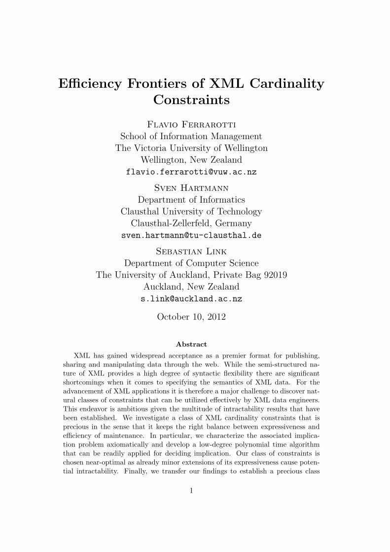
Figure 1: Tree representation of XML data.
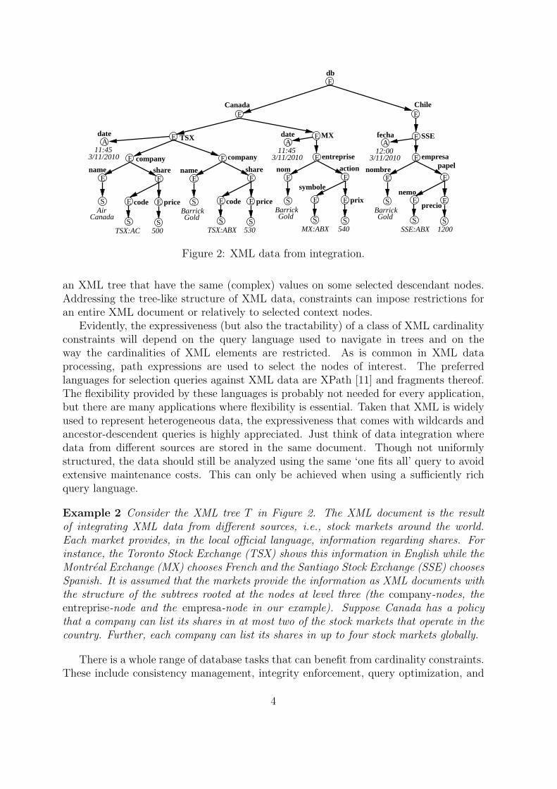
Example 1 Suppose we use XML to store data about bank transactions. Figure 1 showsan artificially small example of such an XML document. In reality there would be ofcourse far more banks, branches, clients, accounts, and transactions. We use the examplejust to illustrate the general structure of the database. Among other information, the date,type (e.g., deposit or withdrawal) and amount of each transaction are registered in thedatabase. Each transaction belongs to an account which belongs to a branch of a givenbank. A cardinality constraint could now state that each bank can handle up to 300, 000transactions per day.
More generally, cardinality constraints restrict the cardinality of the answer to somequery against the database. For any given bank and any given date, we could ask forthe number of transactions registered for this bank and date. The cardinality constraintunder inspection just states that the answer will consist of at most 300, 000 transactions.It is easy to see that occurrence constraints, as defined by XML Schema, are not ex-pressive enough to capture such properties. The reason is that XML Schema occurrenceconstraints simply restrict the number of occurrences of XML elements, independentlyof the data carried by these elements. Instead, a class of constraints is required thatrestricts the number of XML elements dependent on the data that they carry. Such aclass is reminiscent of the cardinality constraints from conceptual modeling [35, 51] andis tailored towards the particularities of XML.
Throughout we will use a simple XML tree model as proposed by DOM [2] and XPath,but independently from schema specifications such as DTDs [7] or XSDs [56]. Figure 2shows a tree representation of an XML data fragment in which nodes are annotated bytheir type: E for elements, A for attributes, and S for text (PCDATA) in XML data.
In this article we study cardinality constraints that restrict the number of nodes in
3
E
E
E
E
S
name
CanadaAir
E
E
S
E
S
E
E
S
E
E
S
E
S
3/11/201011:45
dateA
3/11/201011:45
dateA
E
E
E
S
E
E
S
E
S
Edb
A
E
E
E
E
E
S E
S
E
S
Canada
share
price
500
code
TSX:AC
company
TSX
company
name
BarrickGold
share
pricecode
TSX:ABX 530
MX
BarrickGold
entreprise
nom action
symbole
prix
MX:ABX 540
fecha
12:003/11/2010
BarrickGold
SSE
Chile
empresa
nombre
1200SSE:ABX
nemo
precio
papel
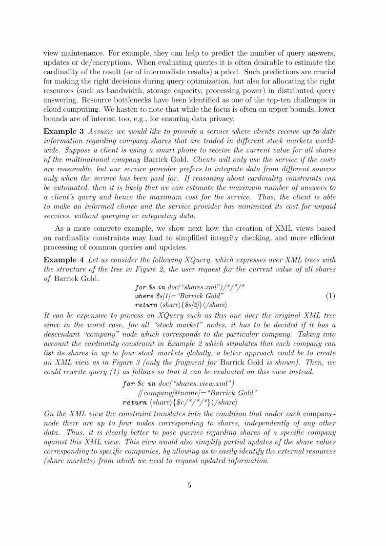
Figure 2: XML data from integration.
an XML tree that have the same (complex) values on some selected descendant nodes.Addressing the tree-like structure of XML data, constraints can impose restrictions foran entire XML document or relatively to selected context nodes.
Evidently, the expressiveness (but also the tractability) of a class of XML cardinalityconstraints will depend on the query language used to navigate in trees and on theway the cardinalities of XML elements are restricted. As is common in XML dataprocessing, path expressions are used to select the nodes of interest. The preferredlanguages for selection queries against XML data are XPath [11] and fragments thereof.The flexibility provided by these languages is probably not needed for every application,but there are many applications where flexibility is essential. Taken that XML is widelyused to represent heterogeneous data, the expressiveness that comes with wildcards andancestor-descendent queries is highly appreciated. Just think of data integration wheredata from different sources are stored in the same document. Though not uniformlystructured, the data should still be analyzed using the same ‘one fits all’ query to avoidextensive maintenance costs. This can only be achieved when using a sufficiently richquery language.
Example 2 Consider the XML tree T in Figure 2. The XML document is the resultof integrating XML data from different sources, i.e., stock markets around the world.Each market provides, in the local official language, information regarding shares. Forinstance, the Toronto Stock Exchange (TSX) shows this information in English while theMontreal Exchange (MX) chooses French and the Santiago Stock Exchange (SSE) choosesSpanish. It is assumed that the markets provide the information as XML documents withthe structure of the subtrees rooted at the nodes at level three (the company-nodes, theentreprise-node and the empresa-node in our example). Suppose Canada has a policythat a company can list its shares in at most two of the stock markets that operate in thecountry. Further, each company can list its shares in up to four stock markets globally.
There is a whole range of database tasks that can benefit from cardinality constraints.These include consistency management, integrity enforcement, query optimization, and
4
view maintenance. For example, they can help to predict the number of query answers,updates or de/encryptions. When evaluating queries it is often desirable to estimate thecardinality of the result (or of intermediate results) a priori. Such predictions are crucialfor making the right decisions during query optimization, but also for allocating the rightresources (such as bandwidth, storage capacity, processing power) in distributed queryanswering. Resource bottlenecks have been identified as one of the top-ten challenges incloud computing. We hasten to note that while the focus is often on upper bounds, lowerbounds are of interest too, e.g., for ensuring data privacy.
Example 3 Assume we would like to provide a service where clients receive up-to-dateinformation regarding company shares that are traded in different stock markets world-wide. Suppose a client is using a smart phone to receive the current value for all sharesof the multinational company Barrick Gold. Clients will only use the service if the costsare reasonable, but our service provider prefers to integrate data from different sourcesonly when the service has been paid for. If reasoning about cardinality constraints canbe automated, then it is likely that we can estimate the maximum number of answers toa client’s query and hence the maximum cost for the service. Thus, the client is ableto make an informed choice and the service provider has minimized its cost for unpaidservices, without querying or integrating data.
As a more concrete example, we show next how the creation of XML views basedon cardinality constraints may lead to simplified integrity checking, and more efficientprocessing of common queries and updates.
Example 4 Let us consider the following XQuery, which expresses over XML trees withthe structure of the tree in Figure 2, the user request for the current value of all sharesof Barrick Gold.
for $s in doc(“shares.xml”)/*/*/*where $s[1]=“Barrick Gold”return ⟨share⟩{$s[2]}⟨/share⟩
(1)
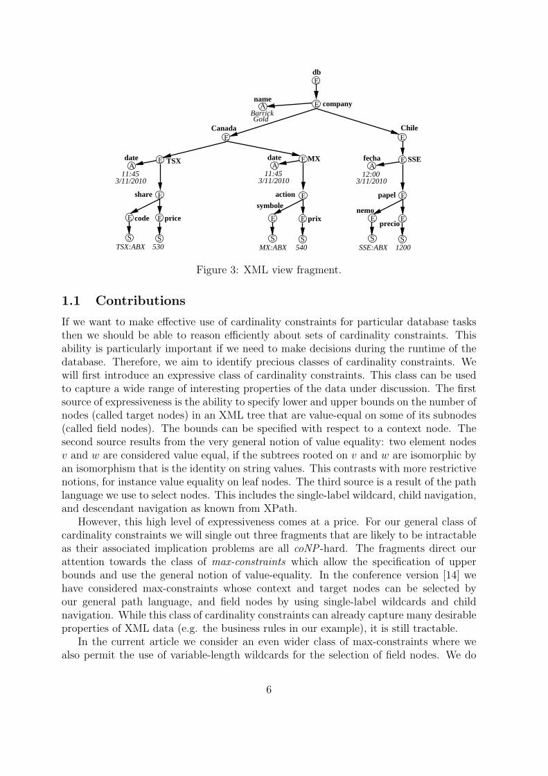
It can be expensive to process an XQuery such as this one over the original XML treesince in the worst case, for all “stock market” nodes, it has to be decided if it has adescendant “company” node which corresponds to the particular company. Taking intoaccount the cardinality constraint in Example 2 which stipulates that each company canlist its shares in up to four stock markets globally, a better approach could be to createan XML view as in Figure 3 (only the fragment for Barrick Gold is shown). Then, wecould rewrite query (1) as follows so that it can be evaluated on this view instead.
for $c in doc(“shares view.xml”)//company[@name]=“Barrick Gold”
return ⟨share⟩{$c/*/*/*}⟨/share⟩On the XML view the constraint translates into the condition that under each company-node there are up to four nodes corresponding to shares, independently of any otherdata. Thus, it is clearly better to pose queries regarding shares of a specific companyagainst this XML view. This view would also simplify partial updates of the share valuescorresponding to specific companies, by allowing us to easily identify the external resources(share markets) from which we need to request updated information.
5
E
E
3/11/201011:45
dateA
EA
E
E
E
Edb
A
3/11/201011:45
dateA
E
E
S
E
S
E
E
S
E
S
E
E
S
E
S
TSX MX fecha
12:003/11/2010
SSE
ChileCanada
companyBarrickGold
code price
TSX:ABX 530
symbole
prix
MX:ABX 540 1200SSE:ABX
nemo
precio
action papelshare
name
Figure 3: XML view fragment.
1.1 Contributions
If we want to make effective use of cardinality constraints for particular database tasksthen we should be able to reason efficiently about sets of cardinality constraints. Thisability is particularly important if we need to make decisions during the runtime of thedatabase. Therefore, we aim to identify precious classes of cardinality constraints. Wewill first introduce an expressive class of cardinality constraints. This class can be usedto capture a wide range of interesting properties of the data under discussion. The firstsource of expressiveness is the ability to specify lower and upper bounds on the number ofnodes (called target nodes) in an XML tree that are value-equal on some of its subnodes(called field nodes). The bounds can be specified with respect to a context node. Thesecond source results from the very general notion of value equality: two element nodesv and w are considered value equal, if the subtrees rooted on v and w are isomorphic byan isomorphism that is the identity on string values. This contrasts with more restrictivenotions, for instance value equality on leaf nodes. The third source is a result of the pathlanguage we use to select nodes. This includes the single-label wildcard, child navigation,and descendant navigation as known from XPath.
However, this high level of expressiveness comes at a price. For our general class ofcardinality constraints we will single out three fragments that are likely to be intractableas their associated implication problems are all coNP -hard. The fragments direct ourattention towards the class of max-constraints which allow the specification of upperbounds and use the general notion of value-equality. In the conference version [14] wehave considered max-constraints whose context and target nodes can be selected byour general path language, and field nodes by using single-label wildcards and childnavigation. While this class of cardinality constraints can already capture many desirableproperties of XML data (e.g. the business rules in our example), it is still tractable.
In the current article we consider an even wider class of max-constraints where wealso permit the use of variable-length wildcards for the selection of field nodes. We do
6
that in a controlled manner so that tractability is still guaranteed. Moreover, we permitthe use of max-constraints that have no field paths: These constraints impose upperbounds on the total number of targets in the scope of a context node. Again we do thatin a controlled way to ensure tractability. This class includes maxOccurs constraints, asdefined by XML Schema, as a special case, but its expressiveness goes far beyond that.
For our new, wider class of max-constraints we characterize the implication problemaxiomatically as well as algorithmically using shortest path methods in a suitable graph.This constitutes a well-founded framework for developing a compact, low-degree polyno-mial time algorithm that decides implication efficiently. Hence, we establish a preciousclass of cardinality constraints that is effective for flexible XML data processing.
Finally, we discuss the use of max-constraints as soft constraints. These constraintsimpose bounds on the average number of targets that are in the scope of the same contextnode and value-equal on their field nodes, but tolerate violations for some targets. Softconstraints are particularly attractive in database practice, where violations to commonrules frequently occur.
1.2 Organization
Section 2 assembles preliminary terminology and formal notation to be used later on.In Section 3 we introduce an expressive class of cardinality constraints and investigatethe tractability of their implication problem. To overcome potential intractability weintroduce the class of max-constraints. In Section 4 we establish a finite set of inferencerules for deriving new max-constraints, and verify its completeness in Section 5. Section 6presents an efficient algorithm for deciding implication. In Section 7 we discuss a weakerinterpretation of max-constraints as soft constraints and show that it is still tractable.In Section 8 we survey some recent work in the literature on cardinality constraints andon database management support for XML that is related to our study here. Section 9concludes our work.
2 Terminology
2.1 The XML Tree Model
Let E denote a countably infinite set of element tags, A a countably infinite set of at-tribute names, and {S} a singleton set denoting text (PCDATA). These sets are pairwisedisjoint. The elements of L = E ∪A ∪ {S} are called labels.
An XML tree is a 6-tuple T = (V, lab, ele, att, val, r) where V is a set of nodes, andlab is a mapping V → L assigning a label to every node in V . A node v ∈ V is anelement node if lab(v) ∈ E, an attribute node if lab(v) ∈ A, and a text node if lab(v) = S.Moreover, ele and att are partial mappings defining the edge relation of T : for any nodev ∈ V , if v is an element node, then ele(v) is a list of element and text nodes, and att(v)is a set of attribute nodes in V . If v is an attribute or text node, then ele(v) and att(v)are undefined. The partial mapping val assigns a string to each attribute and text node:
7
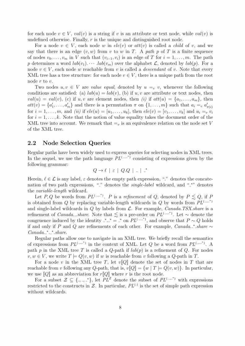
for each node v ∈ V , val(v) is a string if v is an attribute or text node, while val(v) isundefined otherwise. Finally, r is the unique and distinguished root node.
For a node v ∈ V , each node w in ele(v) or att(v) is called a child of v, and wesay that there is an edge (v, w) from v to w in T . A path p of T is a finite sequenceof nodes v0, . . . , vm in V such that (vi−1, vi) is an edge of T for i = 1, . . . ,m. The pathp determines a word lab(v1). · · · .lab(vm) over the alphabet L, denoted by lab(p). For anode v ∈ V , each node w reachable from v is called a descendant of v. Note that everyXML tree has a tree structure: for each node v ∈ V , there is a unique path from the rootnode r to v.
Two nodes u, v ∈ V are value equal, denoted by u =v v, whenever the followingconditions are satisfied: (a) lab(u) = lab(v), (b) if u, v are attribute or text nodes, thenval(u) = val(v), (c) if u, v are element nodes, then (i) if att(u) = {a1, . . . , am}, thenatt(v) = {a′1, . . . , a′m} and there is a permutation π on {1, . . . ,m} such that ai =v a′π(i)for i = 1, . . . ,m, and (ii) if ele(u) = [u1, . . . , uk], then ele(v) = [v1, . . . , vk] and ui =v vifor i = 1, . . . , k. Note that the notion of value equality takes the document order of theXML tree into account. We remark that =v is an equivalence relation on the node set Vof the XML tree.
2.2 Node Selection Queries
Regular paths have been widely used to express queries for selecting nodes in XML trees.In the sequel, we use the path language PL{., , ∗} consisting of expressions given by thefollowing grammar:
Q → ℓ | ε | Q.Q | | ∗
Herein, ℓ ∈ L is any label, ε denotes the empty path expression, “.” denotes the concate-nation of two path expressions, “ ” denotes the single-label wildcard, and “ ∗” denotesthe variable-length wildcard.
Let P,Q be words from PL{., , ∗}. P is a refinement of Q, denoted by P . Q, if Pis obtained from Q by replacing variable-length wildcards in Q by words from PL{., , ∗}
and single-label wildcards in Q by labels from L. For example, Canada.TSX.share is arefinement of Canada. .share. Note that . is a pre-order on PL{., , ∗}. Let ∼ denote thecongruence induced by the identity ∗. ∗ = ∗ on PL{., , ∗}, and observe that P ∼ Q holdsif and only if P and Q are refinements of each other. For example, Canada. ∗.share ∼Canada. ∗. ∗.share.
Regular paths allow one to navigate in an XML tree. We briefly recall the semanticsof expressions from PL{., , ∗} in the context of XML. Let Q be a word from PL{., , ∗}. Apath p in the XML tree T is called a Q-path if lab(p) is a refinement of Q. For nodesv, w ∈ V , we write T |= Q(v, w) if w is reachable from v following a Q-path in T .
For a node v in the XML tree T , let v[[Q]] denote the set of nodes in T that arereachable from v following any Q-path, that is, v[[Q]] = {w | T |= Q(v, w)}. In particular,we use [[Q]] as an abbreviation for r[[Q]] where r is the root node.
For a subset Z ⊆ {., , ∗}, let PLZ denote the subset of PL{., , ∗} with expressionsrestricted to the constructs in Z. In particular, PL{.} is the set of simple path expressionwithout wildcards.
8
Since attribute and text nodes in an XML tree T are always leaves, Q ∈ PL{., , ∗} isvalid only if it has no labels ℓ ∈ A or ℓ = S in a position other than the terminal one.Note that each prefix of a valid Q is valid, too.
Let P,Q be words from PL{., , ∗}. P is contained in Q, denoted by P ⊆ Q, if for everyXML tree T and every node v of T we have v[[P ]] ⊆ v[[Q]]. It follows immediately fromthe definition that P . Q implies P ⊆ Q.
We work with the quotient set PL{., , ∗}/∼ rather than with PL{., , ∗} directly: A word
from PL{., , ∗} is in normal form if it has no consecutive variable-length wildcards, i.e., ifit has no consecutive “ ∗” and no occurrence of “ ∗. ”. Note that, each congruence classcontains a unique word in normal form. Each word from PL{., , ∗} can be transformed intonormal form in linear time, just by removing superfluous variable-length wildcards andreplacing each occurrence of “ ∗. ” by “ . ∗”. The length |Q| of a PL{., , ∗} expression Q isthe number of labels in Q plus the number of wildcards (counting both variable-lengthand single-label wildcards) in the normal form of Q.
The empty path expression ε has length 0. The natural homomorphism from PL{., , ∗}
to PL{., , ∗}/∼ is an isomorphism when restricted to words in normal form. By abuse of
notation we use the words from PL{., , ∗} to denote their respective congruence class.For nodes v and v′ of an XML tree T , the value intersection of v[[Q]] and v′[[Q]] is given
by v[[Q]] ∩v v′[[Q]] = {(w,w′) | w ∈ v[[Q]], w′ ∈ v′[[Q]], w =v w′}. That is, v[[Q]] ∩v v
′[[Q]]consists of all those node pairs in T that are value equal and are reachable from v andv′, respectively, by following Q-paths.
3 From Expressive Towards Precious Classes
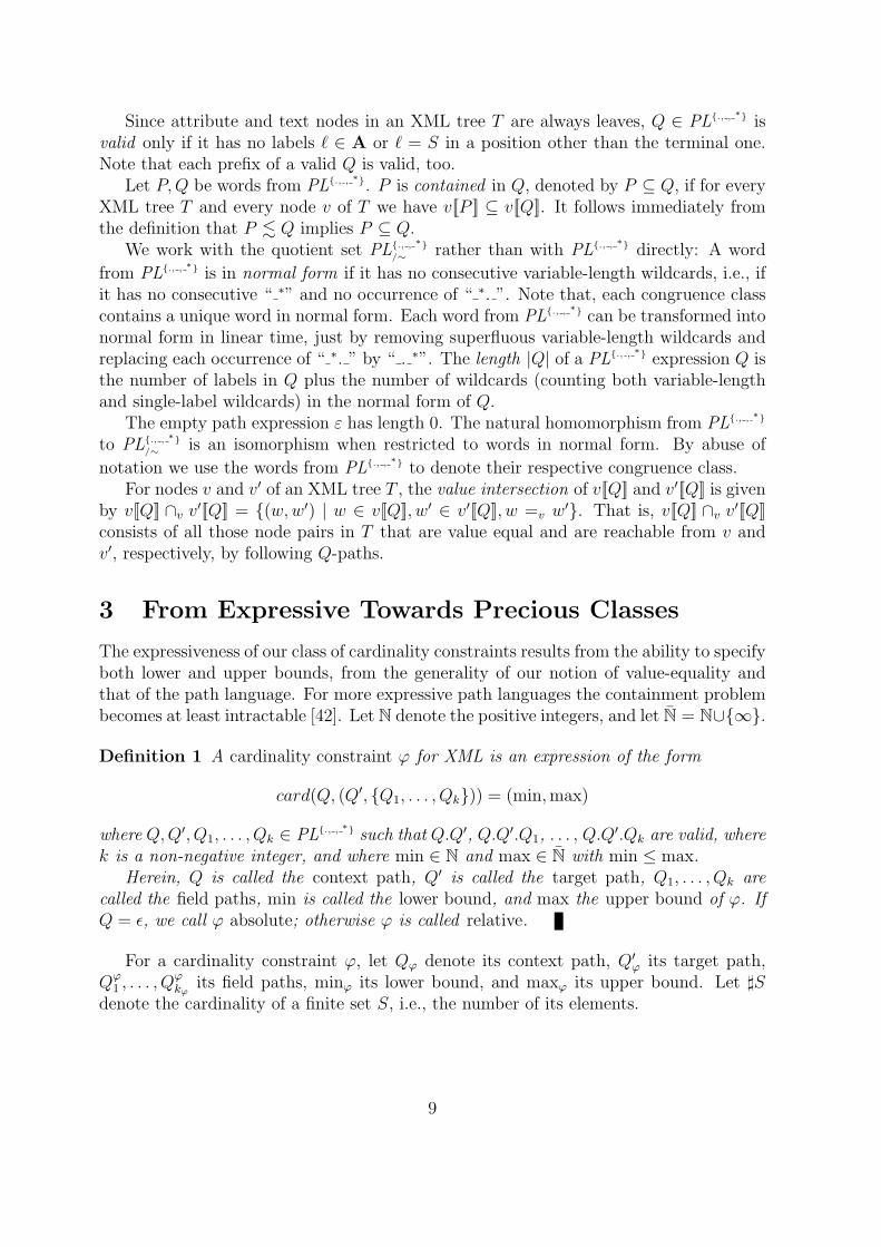
The expressiveness of our class of cardinality constraints results from the ability to specifyboth lower and upper bounds, from the generality of our notion of value-equality andthat of the path language. For more expressive path languages the containment problembecomes at least intractable [42]. Let N denote the positive integers, and let N = N∪{∞}.
Definition 1 A cardinality constraint φ for XML is an expression of the form
card(Q, (Q′, {Q1, . . . , Qk})) = (min,max)
where Q,Q′, Q1, . . . , Qk ∈ PL{., , ∗} such that Q.Q′, Q.Q′.Q1, . . . , Q.Q′.Qk are valid, wherek is a non-negative integer, and where min ∈ N and max ∈ N with min ≤ max.
Herein, Q is called the context path, Q′ is called the target path, Q1, . . . , Qk arecalled the field paths, min is called the lower bound, and max the upper bound of φ. IfQ = ϵ, we call φ absolute; otherwise φ is called relative.
For a cardinality constraint φ, let Qφ denote its context path, Q′φ its target path,
Qφ1 , . . . , Q
φkφ
its field paths, minφ its lower bound, and maxφ its upper bound. Let ♯Sdenote the cardinality of a finite set S, i.e., the number of its elements.
9
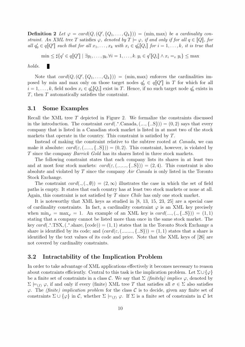
Definition 2 Let φ = card(Q, (Q′, {Q1, . . . , Qk})) = (min,max) be a cardinality con-straint. An XML tree T satisfies φ, denoted by T |= φ, if and only if for all q ∈ [[Q]], forall q′0 ∈ q[[Q′]] such that for all x1, . . . , xk with xi ∈ q′0[[Qi]] for i = 1, . . . , k, it is true that
min ≤ ♯{q′ ∈ q[[Q′]] | ∃y1, . . . , yk.∀i = 1, . . . , k. yi ∈ q′[[Qi]] ∧ xi =v yi} ≤ max
holds.
Note that card(Q, (Q′, {Q1, . . . , Qk})) = (min,max) enforces the cardinalities im-posed by min and max only on those target nodes q′0 ∈ q[[Q′]] in T for which for alli = 1, . . . , k, field nodes xi ∈ q′0[[Qi]] exist in T . Hence, if no such target node q′0 exists inT , then T automatically satisfies the constraint.
3.1 Some Examples
Recall the XML tree T depicted in Figure 2. We formalize the constraints discussedin the introduction. The constraint card( ∗.Canada, ( . , { .S})) = (0, 2) says that everycompany that is listed in a Canadian stock market is listed in at most two of the stockmarkets that operate in the country. This constraint is satisfied by T .
Instead of making the constraint relative to the subtree rooted at Canada, we canmake it absolute: card(ε, ( . . , { .S})) = (0, 2). This constraint, however, is violated byT since the company Barrick Gold has its shares listed in three stock markets.
The following constraint states that each company lists its shares in at least twoand at most four stock markets: card(ε, ( . . ., { .S})) = (2, 4). This constraint is alsoabsolute and violated by T since the company Air Canada is only listed in the TorontoStock Exchange.
The constraint card( , ( , ∅)) = (2,∞) illustrates the case in which the set of fieldpaths is empty. It states that each country has at least two stock markets or none at all.Again, this constraint is not satisfied by T since Chile has only one stock market.
It is noteworthy that XML keys as studied in [8, 13, 15, 23, 25] are a special caseof cardinality constraints. In fact, a cardinality constraint φ is an XML key preciselywhen minφ = maxφ = 1. An example of an XML key is card( . , ( , { .S})) = (1, 1)stating that a company cannot be listed more than once in the same stock market. Thekey card( ∗.TSX, ( ∗.share, {code)) = (1, 1) states that in the Toronto Stock Exchange ashare is identified by its code; and (card(ε, ( . . . , { .S})) = (1, 1) states that a share isidentified by the text values of its code and price. Note that the XML keys of [26] arenot covered by cardinality constraints.
3.2 Intractability of the Implication Problem
In order to take advantage of XML applications effectively it becomes necessary to reasonabout constraints efficiently. Central to this task is the implication problem. Let Σ∪{φ}be a finite set of constraints in a class C. We say that Σ (finitely) implies φ, denoted byΣ |=(f) φ, if and only if every (finite) XML tree T that satisfies all σ ∈ Σ also satisfiesφ. The (finite) implication problem for the class C is to decide, given any finite set ofconstraints Σ ∪ {φ} in C, whether Σ |=(f) φ. If Σ is a finite set of constraints in C let
10
Σ∗(f) denote its (finite) semantic closure, i.e., the set of all constraints (finitely) implied
by Σ. That is, Σ∗(f) = {φ ∈ C | Σ |=(f) φ}.
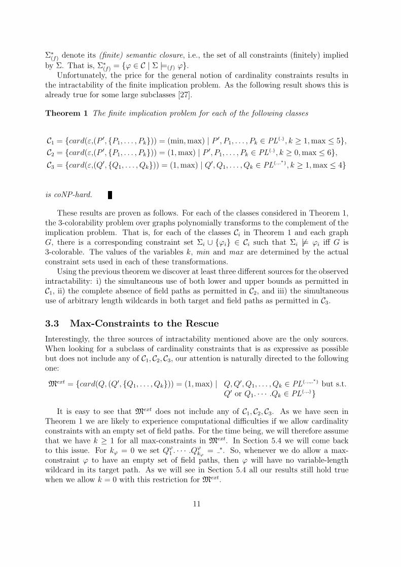
Unfortunately, the price for the general notion of cardinality constraints results inthe intractability of the finite implication problem. As the following result shows this isalready true for some large subclasses [27].
Theorem 1 The finite implication problem for each of the following classes
C1 = {card(ε,(P ′, {P1, . . . , Pk})) = (min,max) | P ′, P1, . . . , Pk ∈ PL{.}, k ≥ 1,max ≤ 5},C2 = {card(ε,(P ′, {P1, . . . , Pk})) = (1,max) | P ′, P1, . . . , Pk ∈ PL{.}, k ≥ 0,max ≤ 6},C3 = {card(ε,(Q′, {Q1, . . . , Qk})) = (1,max) | Q′, Q1, . . . , Qk ∈ PL{., ∗}, k ≥ 1,max ≤ 4}
is coNP-hard.
These results are proven as follows. For each of the classes considered in Theorem 1,the 3-colorability problem over graphs polynomially transforms to the complement of theimplication problem. That is, for each of the classes Ci in Theorem 1 and each graphG, there is a corresponding constraint set Σi ∪ {φi} ∈ Ci such that Σi |= φi iff G is3-colorable. The values of the variables k, min and max are determined by the actualconstraint sets used in each of these transformations.
Using the previous theorem we discover at least three different sources for the observedintractability: i) the simultaneous use of both lower and upper bounds as permitted inC1, ii) the complete absence of field paths as permitted in C2, and iii) the simultaneoususe of arbitrary length wildcards in both target and field paths as permitted in C3.
3.3 Max-Constraints to the Rescue
Interestingly, the three sources of intractability mentioned above are the only sources.When looking for a subclass of cardinality constraints that is as expressive as possiblebut does not include any of C1, C2, C3, our attention is naturally directed to the followingone:
Mext = {card(Q, (Q′, {Q1, . . . , Qk})) = (1,max) | Q,Q′, Q1, . . . , Qk ∈ PL{., , ∗} but s.t.Q′ or Q1. · · · .Qk ∈ PL{., }}
It is easy to see that Mext does not include any of C1, C2, C3. As we have seen inTheorem 1 we are likely to experience computational difficulties if we allow cardinalityconstraints with an empty set of field paths. For the time being, we will therefore assumethat we have k ≥ 1 for all max-constraints in Mext. In Section 5.4 we will come backto this issue. For kφ = 0 we set Qφ
1 . · · · .Qφkφ
= ∗. So, whenever we do allow a max-constraint φ to have an empty set of field paths, then φ will have no variable-lengthwildcard in its target path. As we will see in Section 5.4 all our results still hold truewhen we allow k = 0 with this restriction for Mext.
11

Remark 1 Note that in the conference version [14] of this article we were investigatingthe proper subset M of Mext where the field paths Q1, . . . , Qk are all required to be expres-sions in PL{., }. However, the proof arguments from [14] can be carefully generalized toshow that even the implication problem for the more expressive class Mext can be decidedefficiently.
We give some examples to illustrate the difference between both classes: theconstraint card(ε, ( ∗.account, {transaction. .date.S})) ≤ 100 belongs to the class Mand thus also to the class Mext. On the other hand, the constraint card(ε, ( .account, {transaction. ∗.date.S})) ≤ 100 belongs to the class Mext but not to M. Theconstraint card(ε, ( ∗.account, {transaction . ∗. date.S})) ≤ 100 belongs to neither M norto Mext as it contains variable-length wildcards in the target path and in a field path.
Definition 3 We call Mext the class of max-constraints for XML and use the abbrevi-ation
card(Q, (Q′, {Q1, . . . , Qk})) ≤ max
to denote these constraints.
The classes M and Mext are quite expressive. In particular, they each subsumethe class of XML keys [13] for the special case where maxφ = 1. One of the majorcontributions of the conference version [14] was the inclusion of single-label wildcards inthe definition of max-constraints. We would like to emphasize the significance of thisextension. In fact, this feature adds expressiveness to the language that has importantapplications in data integration.
Example 5 We will illustrate this point by the example from the introduction. Letus consider the constraints φ1 = card( ∗.Canada, ( . , { .S})) ≤ 2 and φ2 =card(ε, ( . . ., { .S})) ≤ 4. That is, every company is listed in at most two of the stockmarkets that operate in Canada, and every company lists its shares in at most four stockmarkets. Clearly, these constraints cannot be expressed without the single-label wildcardwhen we consider trees with the structure of T in Figure 2.
We could represent the same information in a tree T ′ different from T . For example,replacing the element nodes Canada and Chile by element nodes country with attributechildren name where val(name) = Canada and = Chile, respectively; replacing theelement nodes TSX, MX and SSE by element nodes market with attribute children dateand name where val(name) = TSX, = MX, and = SSE, respectively; and replacingall non-English labels of the remaining element nodes by their corresponding Englishtranslation, i.e., replacing empresa by company, papel by share and so on.
Over trees with the structure of T ′, it is easy to check that the constraintcard(ε, (country.market.company, {name.S})) ≤ 4 (without single-label wildcards) isequivalent to φ2. However, φ1 is not meaningful in T ′ and there is no cardinality con-straint φ′
1 such that for every tree Ti with the structure of T and every correspondingequivalent tree T ′
i with the structure of T ′, Ti |= φ1 iff T ′i |= φ′
1. We can replace thecountry-nodes in T ′ with the labels they have in T , but then no constraint without asingle-label wildcard is equivalent to φ2.
12
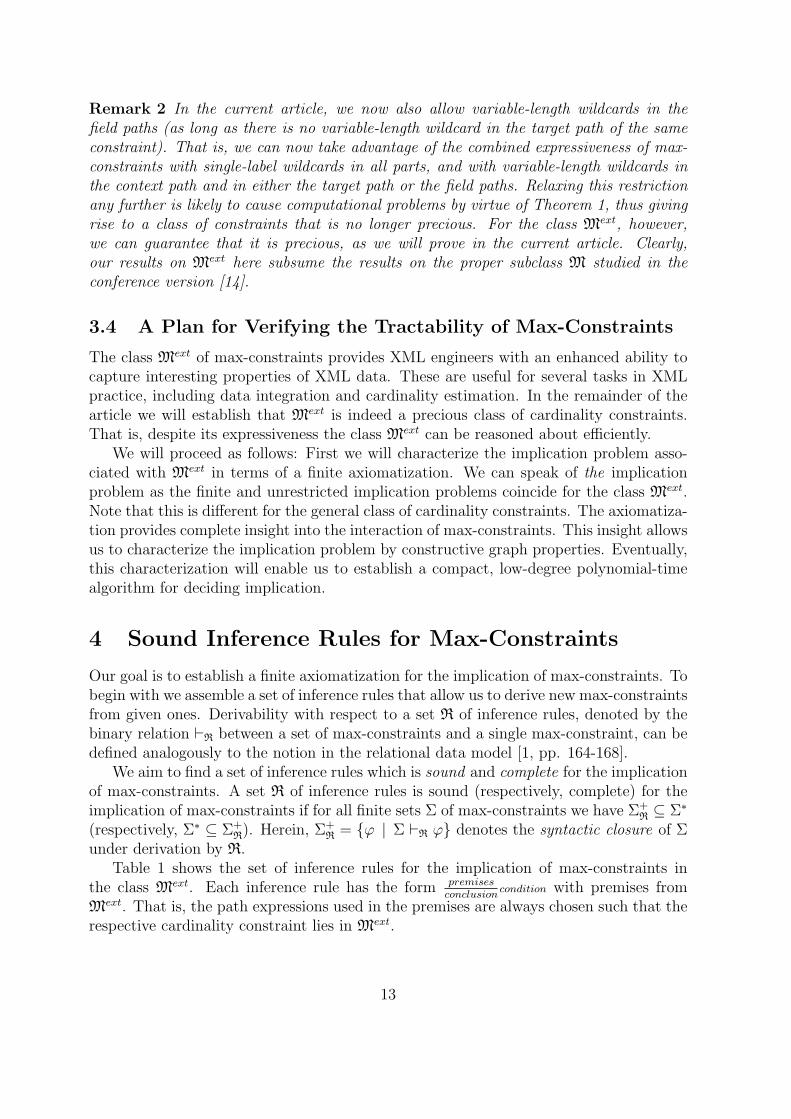
Remark 2 In the current article, we now also allow variable-length wildcards in thefield paths (as long as there is no variable-length wildcard in the target path of the sameconstraint). That is, we can now take advantage of the combined expressiveness of max-constraints with single-label wildcards in all parts, and with variable-length wildcards inthe context path and in either the target path or the field paths. Relaxing this restrictionany further is likely to cause computational problems by virtue of Theorem 1, thus givingrise to a class of constraints that is no longer precious. For the class Mext, however,we can guarantee that it is precious, as we will prove in the current article. Clearly,our results on Mext here subsume the results on the proper subclass M studied in theconference version [14].
3.4 A Plan for Verifying the Tractability of Max-Constraints
The class Mext of max-constraints provides XML engineers with an enhanced ability tocapture interesting properties of XML data. These are useful for several tasks in XMLpractice, including data integration and cardinality estimation. In the remainder of thearticle we will establish that Mext is indeed a precious class of cardinality constraints.That is, despite its expressiveness the class Mext can be reasoned about efficiently.
We will proceed as follows: First we will characterize the implication problem asso-ciated with Mext in terms of a finite axiomatization. We can speak of the implicationproblem as the finite and unrestricted implication problems coincide for the class Mext.Note that this is different for the general class of cardinality constraints. The axiomatiza-tion provides complete insight into the interaction of max-constraints. This insight allowsus to characterize the implication problem by constructive graph properties. Eventually,this characterization will enable us to establish a compact, low-degree polynomial-timealgorithm for deciding implication.
4 Sound Inference Rules for Max-Constraints
Our goal is to establish a finite axiomatization for the implication of max-constraints. Tobegin with we assemble a set of inference rules that allow us to derive new max-constraintsfrom given ones. Derivability with respect to a set R of inference rules, denoted by thebinary relation ⊢R between a set of max-constraints and a single max-constraint, can bedefined analogously to the notion in the relational data model [1, pp. 164-168].
We aim to find a set of inference rules which is sound and complete for the implicationof max-constraints. A set R of inference rules is sound (respectively, complete) for theimplication of max-constraints if for all finite sets Σ of max-constraints we have Σ+
R ⊆ Σ∗
(respectively, Σ∗ ⊆ Σ+R). Herein, Σ
+R = {φ | Σ ⊢R φ} denotes the syntactic closure of Σ
under derivation by R.Table 1 shows the set of inference rules for the implication of max-constraints in
the class Mext. Each inference rule has the form premisesconclusion
condition with premises fromMext. That is, the path expressions used in the premises are always chosen such that therespective cardinality constraint lies in Mext.
13

card(Q, (Q′, S)) ≤ ∞Q′∈PL{., } or ∅=S⊆PL{., }
card(Q, (ϵ, S)) ≤ 1(infinity) (epsilon)
card(Q, (Q′.Q′′, S)) ≤ max
card(Q.Q′, (Q′′, S)) ≤ max
card(Q, (Q′, S)) ≤ max
card(Q, (Q′, S)) ≤ max+1(target-to-context) (weakening)
card(Q, (Q′, S)) ≤ max
card(Q, (Q′, S ∪ {P})) ≤ maxQ′ or P∈PL{., }
card(Q, (Q′, S ∪ {ϵ, P})) ≤ max
card(Q, (Q′, S ∪ {ϵ, P.P ′})) ≤ max(superfield) (prefix-epsilon)
card(Q, (Q′.P, {P ′})) ≤ max
card(Q, (Q′, {P.P ′})) ≤ maxat least 2 of Q′, P, P ′ ∈ PL{., }
card(Q, (Q′, S)) ≤ max
card(Q′′, (Q′, S)) ≤ maxQ′′⊆Q
(subnodes) (context-path-containment)
card(Q, (Q′.P, {ϵ, P ′})) ≤ max
card(Q, (Q′, {ϵ, P.P ′})) ≤ maxat least 2 of Q′, P, P ′ ∈ PL{., }
card(Q, (Q′, S)) ≤ max
card(Q, (Q′′, S)) ≤ maxQ′′⊆Q′
(subnodes-epsilon) (target-path-containment)
card(Q, (Q′, {P.P1, . . . , P.Pk})) ≤ max,card(Q.Q′, (P, {P1, . . . , Pk})) ≤ max′
card(Q, (Q′.P, {P1, . . . , Pk})) ≤ max ·max′card(Q, (Q′, S ∪ {P})) ≤ max
card(Q, (Q′, S ∪ {P ′})) ≤ maxP ′⊆P
(multiplication) (field-path-containment)
Table 1: A Finite Axiomatization for Max-constraints in Mext.
We prove below the soundness of the field-path containment rule and the subnodesrule. The soundness of the remaining rules can be shown using similar arguments. There-fore we omit those lengthy, but not very difficult proofs. For comparison, we also referto our soundness proofs in [27] for the special case where no single-label wildcards arepermitted, and variable-length wildcards are permitted to occur only in the context andtarget paths.
Lemma 1 The field-path containment rule is sound for the implication of max-constraints in the class Mext.
Proof Suppose an XML tree T violates card(Q, (Q′, S ∪ {P ′})) ≤ max. Let S ∪ {P ′} ={P1, . . . , Pk} such that Pk = P ′ with k ≥ 1. Then there is some node q ∈ [[Q]] and somenode q′0 ∈ q[[Q′]] such that for some x1, . . . , xk with xi ∈ q′0[[Pi]] for i = 1, . . . , k, it holdsthat
♯{q′ ∈ q[[Q′]] | ∃y1, . . . , yk.∀i = 1, . . . , k. yi ∈ q′[[Pi]] ∧ xi =v yi} > max .
However, since P ′ = Pk ⊆ P , for every q′ ∈ q[[Q′]] it holds that there is a yk ∈ q′[[Pk]]with xk =v yk if it also holds that yk ∈ q′[[P ]]. But then it is easy to see that there are
14

x1, . . . , xk with xi ∈ q′0[[Pi]] for i = 1, . . . , k − 1 and xk ∈ q′0[[P ]] such that
♯{q′ ∈ q[[Q′]] | ∃y1, . . . , yk.∀i = 1, . . . , k − 1.yi ∈ q′[[Pi]]∧yk ∈ q′[[P ]] ∧ xi =v yi ∧ xk =v yk} > max .
This shows that T also violates σ = card(Q, (Q′, S ∪ {P})) ≤ max.
Lemma 2 The subnodes rule is sound for the implication of max-constraints in the classMext.
Proof Suppose an XML tree T violates card(Q, (Q′, {P.P ′})) ≤ max. Then there issome node q ∈ [[Q]] and some node q′0 ∈ q[[Q′]] such that for some x ∈ q′0[[P.P
′]] it holdsthat
♯{q′ ∈ q[[Q′]] | ∃y.y ∈ q′[[P.P ′]] ∧ x =v y} > max .
For every pair of distinct nodes q′i and q′j in the previous set, it also holds that q′i isneither an ancestor nor a descendant of q′j. This holds true, since T is a tree and dueto the condition of the subnodes rule Q′ or P.P ′ is a PL{., } expression, that is, has novariable-length wild cards. Consequently, we have
♯{p ∈ q[[Q′.P ]] | ∃y.y ∈ p[[P ′]] ∧ x =v y} > max .
This shows that T also violates σ = card(Q, (Q′.P, {P ′})) ≤ max.
Remark 3 In the proof of the previous lemma we have made an interesting observation:If we allow the use of variable-length wildcards in the target and field paths at the sametime, then we could have a pair of distinct target nodes in the set {q′ ∈ q[[Q′]] | ∃y.y ∈q′[[P.P ′]] ∧ x =v y} so that one is an ancestor of the other one. This would allow us tobuild a counterexample tree to demonstrate that the subnodes rule is not sound for suchan extended class of max-constraints. However, we do not study this case any furthersince the implication problem becomes intractable as seen in Theorem 1.
5 Axiomatic Characterization of Implication
Our goal is to demonstrate that the set R of inference rules is also complete for theimplication of max-constraints in the class Mext. Completeness means we need to showthat for an arbitrary finite set Σ∪{φ} of max-constraints in the class Mext with φ /∈ Σ+
R
there is some XML tree T that satisfies all members of Σ but violates φ. That is, T is acounter-example tree for the implication of φ by Σ.
The general proof strategy is as follows: For T to be a counter-example we i) require acontext node qφ with more than maxφ target nodes q′φ that all have value-equal field nodesqφ1 , . . . , q
φkφ, and ii) must for each context node qσ not have more than maxσ target nodes
q′σ that all have value-equal field nodes qσ1 , . . . , qσkσ, for each member σ of Σ. Basically,
such a counter-example tree exists if and only if these two conditions can be satisfiedsimultaneously. In a first step, we represent φ as a finite node-labeled tree TΣ,φ, whichwe call the mini-tree.
15

Then, we reverse the edges of the mini-tree and add to the resulting tree downwardedges for certain members of Σ. Finally, each upward edge receives a label of 1 and eachdownward edge resulting from σ ∈ Σ a label of maxσ. This final digraph GΣ,φ is called thecardinality network. A downward edge resulting from σ tells us that under each sourcenode there can be at most maxσ target nodes. Now, if we can reach the target node of φfrom its context node along a dipath of weight (the product of its labels) at most maxφ,then there is no counter-example tree T . In other words, if we satisfy condition ii) above,then we cannot satisfy condition i). Otherwise, we can construct a counter-example treeT .
5.1 Cardinality Networks
Let Σ ∪ {φ} be a finite set of max-constraints in the class Mext. Let LΣ,φ denote theset of all labels ℓ ∈ L that occur in path expressions of members in Σ ∪ {φ}, and fix alabel ℓ0 ∈ E− LΣ,φ. First we transform the path expressions occurring in φ into simplepath expressions in PL{.}. For that purpose we replace each single-label wildcard “ ” byℓ0 and each variable-length wildcard “ ∗” by a sequence of l + 1 labels ℓ0, where l is themaximum number of consecutive single-label wildcards that occurs in any constraint inΣ ∪ {φ}. This transformation turns Qφ into Oφ, Q
′φ into O′
φ, and each Qφi into Oφ
1 fori = 1, . . . , kφ. The path expressions after the transformation do not contain any morewildcards (neither single-label nor variable-length ones).
The proper choice of the integer l is essential for the later construction. In partic-ular, if there are no occurrences of single-label wildcards in the max-constraints underconsideration, then l = 0 and we just replace each variable-length wildcard “ ∗” by oneℓ0.
To continue with our construction, let p be an Oφ-path from a node rφ to a nodeqφ, let p
′ be an O′φ-path from a node r′φ to a node q′φ and, for i = 1, . . . , kφ, let pi be a
Oφi -path from a node rφi to a node xφ
i , such that the paths p, p′, p1, . . . , pkφ are mutuallynode-disjoint. From the paths p, p′, p1, . . . , pkφ we obtain the mini-tree TΣ,φ by identifyingthe node r′φ with qφ, and by identifying each of the nodes rφi with q′φ.
The marking of the mini-tree TΣ,φ is a subset M of the node set of TΣ,φ: if for alli = 1, . . . , kφ we have Qφ
i = ε, then M consists of the leaves of TΣ,φ, and otherwise Mconsists of all descendant nodes of q′φ in TΣ,φ.
We use mini-trees to calculate the impact of max-constraints in Σ on a possiblecounter-example tree for the implication of φ by Σ. To distinguish max-constraintsthat have an impact from those that do not, we introduce the notion of applicability.Intuitively, when a max-constraint is not applicable, then we do not need to satisfy itsupper bound in a counter-example tree as it does not require all its field paths. Let TΣ,φ
be the mini-tree of the max-constraint φ with respect to Σ, and let M be its marking.A max-constraint σ is said to be applicable to φ if there are nodes wσ ∈ [[Qσ]] andw′
σ ∈ wσ[[Q′σ]] in TΣ,φ such that w′
σ[[Pσi ]] ∩M = ∅ for all i = 1, . . . , kσ. We say that wσ
and w′σ witness the applicability of σ to φ.
Example 6 Let us consider an XML database for projects of a company. A year isdivided into quarters and each quarter contains a sequence of projects. Each project
16
E
E
E
E
E
E
E
E
S1
db
label
label
year
quarter
project
1
1
1
1
1
eid1
2
3
label
1
1E
E
E
E
E
E
S1
E
E
E
E
E
E
E
E
S
db
label
label
year
quarter
project
label
eid
x
E
E
E
E
E
E
E
E
E
E
E
E
S
E
E
E
S
E
E
E
E
E l1
E
db
label
label
yearl2
E
label
1
label
year
quarter
project
1
1
1
1
eid1
2
3
db
first
p1 p2
l31 l32
l41 l42
100 100
E E
quarter quarter
projectproject
label
eid eid
label
2010
second
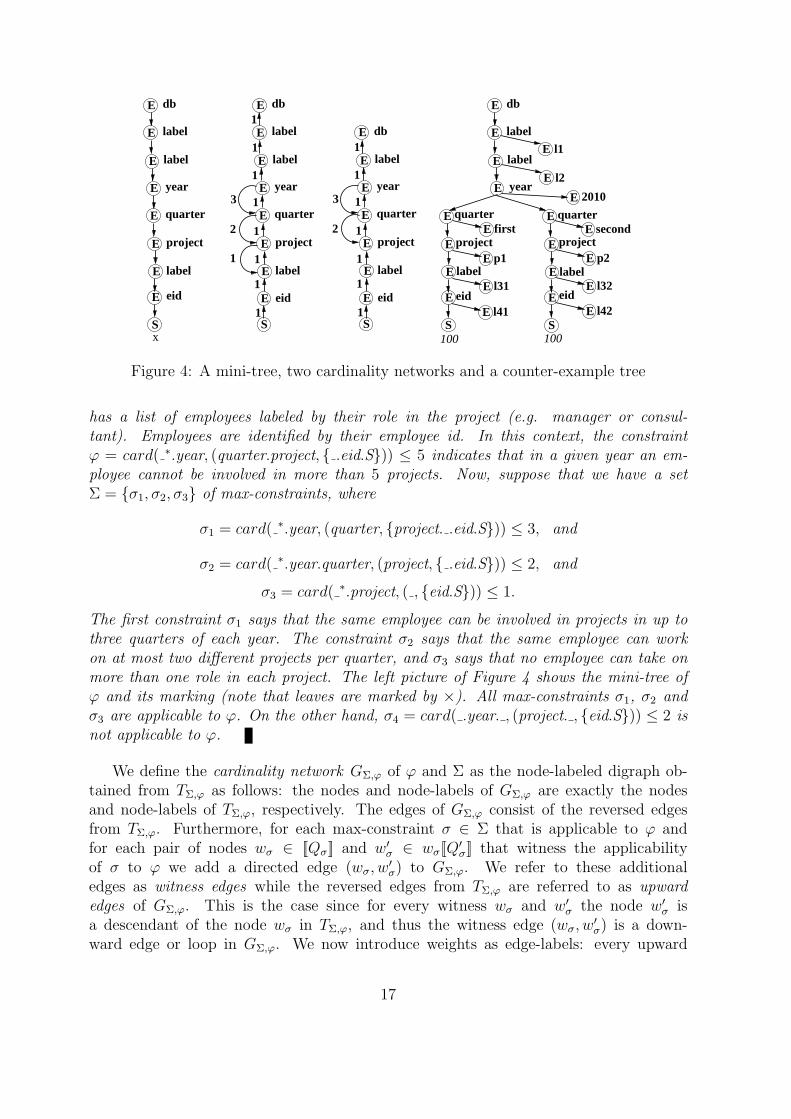
Figure 4: A mini-tree, two cardinality networks and a counter-example tree
has a list of employees labeled by their role in the project (e.g. manager or consul-tant). Employees are identified by their employee id. In this context, the constraintφ = card( ∗.year, (quarter.project, { .eid.S})) ≤ 5 indicates that in a given year an em-ployee cannot be involved in more than 5 projects. Now, suppose that we have a setΣ = {σ1, σ2, σ3} of max-constraints, where
σ1 = card( ∗.year, (quarter, {project. .eid.S})) ≤ 3, and
σ2 = card( ∗.year.quarter, (project, { .eid.S})) ≤ 2, and
σ3 = card( ∗.project, ( , {eid.S})) ≤ 1.
The first constraint σ1 says that the same employee can be involved in projects in up tothree quarters of each year. The constraint σ2 says that the same employee can workon at most two different projects per quarter, and σ3 says that no employee can take onmore than one role in each project. The left picture of Figure 4 shows the mini-tree ofφ and its marking (note that leaves are marked by ×). All max-constraints σ1, σ2 andσ3 are applicable to φ. On the other hand, σ4 = card( .year. , (project. , {eid.S})) ≤ 2 isnot applicable to φ.
We define the cardinality network GΣ,φ of φ and Σ as the node-labeled digraph ob-tained from TΣ,φ as follows: the nodes and node-labels of GΣ,φ are exactly the nodesand node-labels of TΣ,φ, respectively. The edges of GΣ,φ consist of the reversed edgesfrom TΣ,φ. Furthermore, for each max-constraint σ ∈ Σ that is applicable to φ andfor each pair of nodes wσ ∈ [[Qσ]] and w′
σ ∈ wσ[[Q′σ]] that witness the applicability
of σ to φ we add a directed edge (wσ, w′σ) to GΣ,φ. We refer to these additional
edges as witness edges while the reversed edges from TΣ,φ are referred to as upwardedges of GΣ,φ. This is the case since for every witness wσ and w′
σ the node w′σ is
a descendant of the node wσ in TΣ,φ, and thus the witness edge (wσ, w′σ) is a down-
ward edge or loop in GΣ,φ. We now introduce weights as edge-labels: every upward
17

edge e of GΣ,φ has weight ω(e) = 1, and every witness edge (u, v) of GΣ,φ has weightω(u, v) = min{maxσ | (u, v) witnesses the applicability of some σ ∈ Σ to φ}.
We need to use some graph terminology, cf. [31]. Consider some digraph G. A path tis a sequence v0, . . . , vm of nodes with an edge (vi−1, vi) for each i = 1, . . . ,m. We call ta path of length m from node v0 to node vm containing the edges (vi−1, vi), i = 1, . . . ,m.A simple path is just a path whose nodes are pairwise distinct. Note that for every pathfrom u to v there is also a simple path from u to v in G containing only edges of thepath. In the cardinality network GΣ,φ the weight of a path t is defined as the product
of the weights of its edges, i.e., ω(t) =n∏
i=1
ω(vi−1, vi), or ω(t) = 1 if t has no edges. The
distance d(v, w) from a node v to a node w is the minimum over the weights of all pathsfrom v to w, or ∞ if no such path exists.
Example 7 Let Σ and φ be as in Example 6. The cardinality network of Σ and φ isillustrated in the second picture from the left in Figure 4. Let v denote the unique year-node, w the unique project-node, and u the unique eid-node in the second picture fromthe left in Figure 4. Then d(v, w) = 6 and d(v, u) = ∞.
In the following section we will prove the following crucial fact. If the distance d(qφ, q′φ)
from qφ to q′φ in GΣ,φ is at most maxφ, then φ ∈ Σ+R. In other words, if φ is not derivable
from Σ, then every path from qφ to q′φ in GΣ,φ has distance at least maxφ + 1.
Example 8 Let φ′ = card( ∗.year, (quarter.project, { .eid.S})) ≤ 6 and Σ be as in Exam-ple 6. The corresponding mini-tree and cardinality network are shown as first and secondpicture from the left in Figure 4, respectively. Since d(qφ, q
′φ) ≤ 6, it follows by Lemma 3
that φ′ is derivable from Σ. In fact, φ′ is clearly derivable by a single application of themultiplication rule to σ1 and σ2.
5.2 Encoding Inferences as Shortest Paths
Our next result states that we can inspect the cardinality network constructed above toderive new max-constraints from the ones given in Σ. This makes the cardinality networka useful tool for computing new max-constraints that is more convenient to handle thanthe inference rules in Table 1.
Lemma 3 Let Σ ∪ {φ}, where φ = card(Qφ, (Q′φ, {Q
φ1 , . . . , Q
φkφ})) ≤ maxφ, be a fi-
nite set of max-constraints in the class Mext. If the distance d(qφ, q′φ) ≤ maxφ in the
cardinality network GΣ,φ, then card(Qφ, (Q′φ, {Q
φ1 , . . . , Q
φkφ})) ≤ maxφ ∈ Σ+
R.
The strategy to prove this lemma is to encode an inference by R by witness edges ofthe cardinality network. We use the following example to illustrate the main steps of theproof.
Example 9 Let us consider an XML database for bank transactions. Among other in-formation, the date of each transaction is registered in this database. Each transaction
18

belongs to an account which belongs to a branch of a given bank. In this context, themax-constraint
φ = card(bank, (branch. ∗.account.transaction, { .date.S})) ≤ 300, 000
indicates that each bank can handle up to 300, 000 transactions per day. Suppose that wehave a set of max-constraints Σ = {σ1, σ2}, where
σ1 = card(ε, ( ∗.account, {transaction. .date.S})) ≤ 100, and
σ2 = card( ∗.branch, ( ∗.transaction. .date, { })) ≤ 3, 000
The first constraint σ1 says that in any given day, an individual account can be involvedin at most 100 transaction. The constraint σ2 says that any given bank branch can processup to a maximum of 3, 000 transactions per day.
We will formally prove Lemma 3 following a top-down approach. Thus, we start bylaying out the strategy of the proof and leave the technical details for later.
Proof Due to the infinity rule there is nothing to show if maxφ = ∞. Assume maxφ <∞. If d(qφ, q
′φ) ≤ maxφ, then let D denote the simple path in GΣ,φ from qφ to q′φ with
ω(D) = d(qφ, q′φ). According to the definition of the cardinality network we can assume
without loss of generality that D consists of a sequence π1, . . . , πn+1, n ≥ 1, where foreach i = 1, . . . , n, πi starts with a possibly empty sequence of upward edges each ofweight 1 followed by a single witness edge (wσi
, w′σi) labeled with maxσi
where wσiand
w′σi
witness the applicability of σi to φ, and πn+1 is a possibly empty sequence of upwardedges labeled with 1. Moreover, we can assume that qφ, w
′σ1, . . . , w′
σnform a proper
descendant chain, q′φ is a proper descendant of w′σn−1
and w′σn
is a descendant node ofq′φ in TΣ,φ. This situation is illustrated by the cardinality network GΣ,φ correspondingto Example 9 which is depicted in Figure 5. Note that d(qφ, q
′φ) = 300, 000 and that the
thick arrows show the path D from qφ to q′φ with ω(D) = d(qφ, q′φ).
E E E E E E E E Edb 1 1 1
bank
label
label
branch
account
transaction
1 1 1
label
date
S1 1 1
3000100
Figure 5: Example 9:Cardinality network
We now describe a series of assumptions which we use to show that the existenceof the witness edges in D implies the existence of a witness edge (qφ, q
′φ) whose weight
is that of the original path D and which results from a max-constraint σ in Σ+. Weformally prove that each of these assumptions hold in A afterwards.
19

1. The final witness edge in D can be replaced by a witness edge that ends in q′φ. Thatis, we can assume without loss of generality that πn+1 is indeed an empty sequenceand w′
σn= q′φ where the set of field paths of σn is {Qφ
1 , . . . , Qφkφ}. In our example,
this means that we can assume the existence of an implied max-constraint thatdetermines the witness edge denoted with a dashed arrow in Figure 6.
E E E E E E E E Edb bank
label
label
branch
account
transaction
label
dateS
3000100
3000
1 1 1 1 1 1 11 1
Figure 6: Example 9: Implied witness edge derived from Assumption 1
2. If there is a witness edge (wσ, w′σ) in the cardinality network GΣ,φ that corresponds
to the applicability of some σ ∈ Σ+R to φ, then for each node w between wσ and
w′σ in TΣ,φ there is also a witness edge (w,w′
σ) in GΣ,φ with ω(wσ, w′σ) = ω(w,w′
σ)which corresponds to the applicability of some σ′ ∈ Σ+
R to φ. In particular, the twowitness edges denoted with dashed arrows in Figure 7, follow from this assumption.
E E E E E E E E Edb bank
label
label
branch
account
transaction
label
date
S1 1 1 1 1 1 11 1
3000100
3000100
Figure 7: Example 9: Implied witness edges derived from Assumption 2
3. If there is a witness edge (wσ1 , w′σ1) with weight maxσ1 and another witness edge
(w′σ1, q′φ) with weight maxσ2 , then there is also a witness edge (wσ1 , q
′φ) with weight
maxσ1 · maxσ2 . An implied witness edge that can be derived by applying thisassumption to our example is shown in Figure 8.
From Assumption 1 and 2, we can conclude that there is a simple path D′ in GΣ,φ
from qφ to q′φ and ω(D) = ω(D′). In fact, D′ consists of the sequence π′1, . . . , π
′n where
each π′i with 1 ≤ i ≤ n consists of a single witness edge (wσi
, w′σi) labeled with maxσi
andwhere w′
σi= wσi+1
for i = 1, . . . , n−1 and wσ1 = qφ and w′σn
= q′φ. Again, qφ, w′σ1, . . . , w′
σn
form a proper descendant chain.
20

E E E E E E E E Edb bank
label
label
branch
account
transaction
label
date
S1 1 1 1 1 1 11 1
100 3000
300,000
Figure 8: Example 9: Implied witness edge derived from Assumption 3
At this stage we can use Assumption 3 repeatedly to conclude that there is a singlewitness edge D0 = (qφ, q
′φ) in GΣ,φ resulting from the max-constraint
σ = card(Qσ, (Q′σ, {Q
φ1 , . . . , Q
φkφ})) ≤
n∏i=1
maxσi∈ Σ+
R
that is applicable to φ. Due to the applicability of σ to φ we conclude that Qφ ⊆ Qσ andQ′
φ ⊆ Q′σ. We can now apply the context-path-containment and target-path-containment
rule to obtain
card(Qφ, (Q′φ, {Q
φ1 , . . . , Q
φkφ})) ≤
n∏i=1
maxσi∈ Σ+
R.
Since
w(D0) =n∏
i=1
maxσi= ω(D) = d(qφ, q
′φ) ≤ maxφ
holds, applications of the weakening rule show that also
card(Qφ, (Q′φ, {Q
φ1 , . . . , Q
φkφ})) ≤ maxφ ∈ Σ+
R
holds which proves the lemma.
5.3 Establishing Completeness
We have now the tools to prove the completeness of our set of inference rules.
Theorem 2 The inference rules in Table 1 are complete for the implication of max-constraints in Mext.
Proof Let Σ∪{φ} be a finite set of max-constraints in the class Mext such that φ /∈ Σ+R.
We construct a finite XML tree T which satisfies all max-constraints in Σ but does notsatisfy φ. Since φ /∈ Σ+
R every existing path from qφ to q′φ in GΣ,φ has weight at leastmaxφ + 1. For each node n in GΣ,φ let ω′(n) = ω(D) where D denotes the shortest pathfrom qφ to n in GΣ,φ, or ω′(n) = maxφ + 1 if there is no such path. In particular, wehave ω′(qφ) = 1 and ω′(q′φ) > maxφ. Let T0 be a copy of the path from the root node rto qφ in TΣ,φ. We extend T0 as follows: for each node n on the path from qφ to q′φ in TΣ,φ
we introduce ω′(n) copies n1, . . . , nω′(n) into T0. Suppose T0 has been constructed down
21
E
E
E
E
E l1
E
db
label
label
yearl2
E 2010
EE
EE
EE
E
EE
E
S
EE
E
S
EE
E
S
EE
E
S
EE
E
S
EE
E
S
quarterfirst
quarter quartersecond third
E
p1
l41
100
project
label
eid E
100
project
label
eid E
100
project
label
eid E
100
project
label
eid E
100
project
label
eid E
100
project
label
eid
p2 p3 p4 p5 p6
E E E E E
EEEEEE
l31 l32 l33 l34 l35 l36
l42 l43 l44 l45 l46
Figure 9: Counter-example tree for the implication of φ by Σ from Example 10.
to the level of u1, . . . , uω′(u) corresponding to node u in TΣ,φ, and let v be the uniquesuccessor of u in TΣ,φ. Then ω′(u) ≤ ω′(v) due to the upward edges in GΣ,φ. For alli = 1, . . . , ω′(u) and all j = 1, . . . , ω′(v) we introduce a new edge (ui, vj) in T if and onlyif j is congruent to i modulo ω′(u). Eventually, T0 has ω′(q′φ) > maxφ leaves.
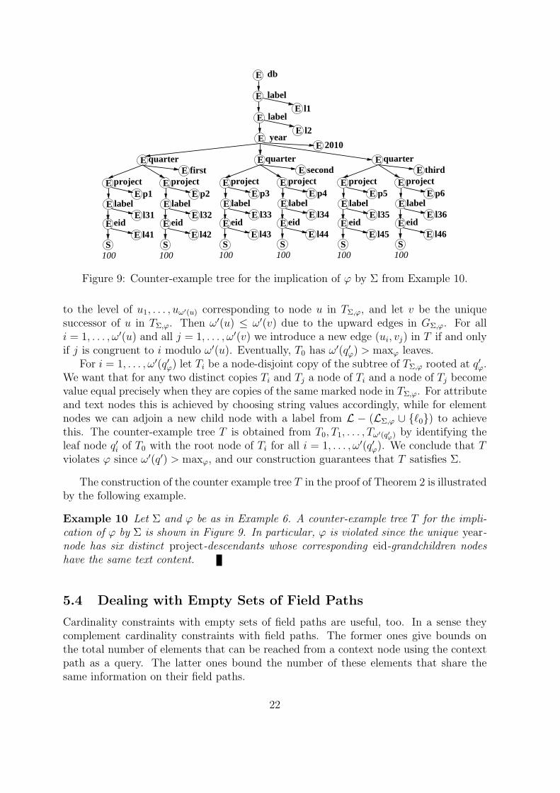
For i = 1, . . . , ω′(q′φ) let Ti be a node-disjoint copy of the subtree of TΣ,φ rooted at q′φ.We want that for any two distinct copies Ti and Tj a node of Ti and a node of Tj becomevalue equal precisely when they are copies of the same marked node in TΣ,φ. For attributeand text nodes this is achieved by choosing string values accordingly, while for elementnodes we can adjoin a new child node with a label from L − (LΣ,φ ∪ {ℓ0}) to achievethis. The counter-example tree T is obtained from T0, T1, . . . , Tω′(q′φ) by identifying theleaf node q′i of T0 with the root node of Ti for all i = 1, . . . , ω′(q′φ). We conclude that Tviolates φ since ω′(q′) > maxφ, and our construction guarantees that T satisfies Σ.
The construction of the counter example tree T in the proof of Theorem 2 is illustratedby the following example.
Example 10 Let Σ and φ be as in Example 6. A counter-example tree T for the impli-cation of φ by Σ is shown in Figure 9. In particular, φ is violated since the unique year-node has six distinct project-descendants whose corresponding eid-grandchildren nodeshave the same text content.
5.4 Dealing with Empty Sets of Field Paths
Cardinality constraints with empty sets of field paths are useful, too. In a sense theycomplement cardinality constraints with field paths. The former ones give bounds onthe total number of elements that can be reached from a context node using the contextpath as a query. The latter ones bound the number of these elements that share thesame information on their field paths.
22
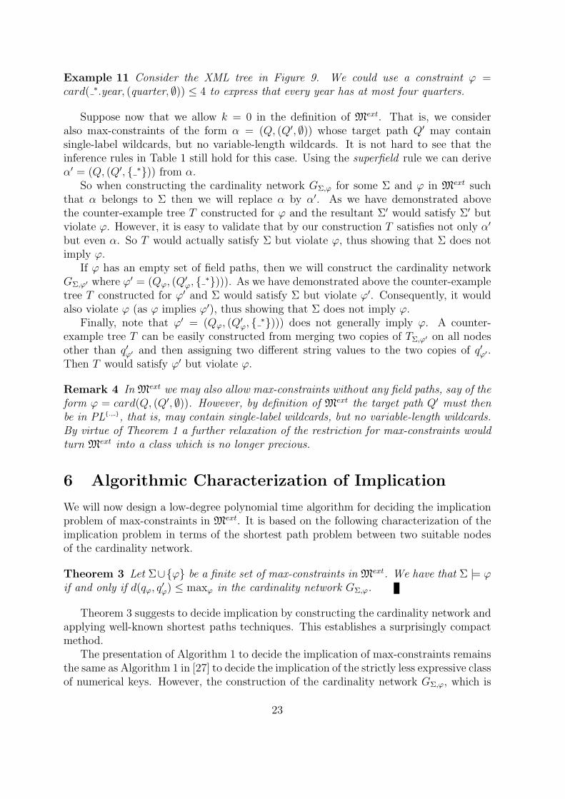
Example 11 Consider the XML tree in Figure 9. We could use a constraint φ =card( ∗.year, (quarter, ∅)) ≤ 4 to express that every year has at most four quarters.
Suppose now that we allow k = 0 in the definition of Mext. That is, we consideralso max-constraints of the form α = (Q, (Q′, ∅)) whose target path Q′ may containsingle-label wildcards, but no variable-length wildcards. It is not hard to see that theinference rules in Table 1 still hold for this case. Using the superfield rule we can deriveα′ = (Q, (Q′, { ∗})) from α.
So when constructing the cardinality network GΣ,φ for some Σ and φ in Mext suchthat α belongs to Σ then we will replace α by α′. As we have demonstrated abovethe counter-example tree T constructed for φ and the resultant Σ′ would satisfy Σ′ butviolate φ. However, it is easy to validate that by our construction T satisfies not only α′
but even α. So T would actually satisfy Σ but violate φ, thus showing that Σ does notimply φ.
If φ has an empty set of field paths, then we will construct the cardinality networkGΣ,φ′ where φ′ = (Qφ, (Q
′φ, { ∗}))). As we have demonstrated above the counter-example
tree T constructed for φ′ and Σ would satisfy Σ but violate φ′. Consequently, it wouldalso violate φ (as φ implies φ′), thus showing that Σ does not imply φ.
Finally, note that φ′ = (Qφ, (Q′φ, { ∗}))) does not generally imply φ. A counter-
example tree T can be easily constructed from merging two copies of TΣ,φ′ on all nodesother than q′φ′ and then assigning two different string values to the two copies of q′φ′ .Then T would satisfy φ′ but violate φ.
Remark 4 In Mext we may also allow max-constraints without any field paths, say of theform φ = card(Q, (Q′, ∅)). However, by definition of Mext the target path Q′ must thenbe in PL{., }, that is, may contain single-label wildcards, but no variable-length wildcards.By virtue of Theorem 1 a further relaxation of the restriction for max-constraints wouldturn Mext into a class which is no longer precious.
6 Algorithmic Characterization of Implication
We will now design a low-degree polynomial time algorithm for deciding the implicationproblem of max-constraints in Mext. It is based on the following characterization of theimplication problem in terms of the shortest path problem between two suitable nodesof the cardinality network.
Theorem 3 Let Σ∪{φ} be a finite set of max-constraints in Mext. We have that Σ |= φif and only if d(qφ, q
′φ) ≤ maxφ in the cardinality network GΣ,φ.
Theorem 3 suggests to decide implication by constructing the cardinality network andapplying well-known shortest paths techniques. This establishes a surprisingly compactmethod.
The presentation of Algorithm 1 to decide the implication of max-constraints remainsthe same as Algorithm 1 in [27] to decide the implication of the strictly less expressive classof numerical keys. However, the construction of the cardinality network GΣ,φ, which is
23

Algorithm 1 Max-constraint implication
1: procedure Decide-Implication(Σ ∪ {φ})2: Construct GΣ,φ for Σ and φ;3: Find the shortest path P from qφ to q′φ in GΣ,φ;4: if ω(P ) ≤ maxφ then5: return(yes);6: else7: return(no);8: end if9: end procedure
central to both algorithms, requires considerably more effort for the more expressive classof max-constraints. This effort results in an increase in the worst-case time complexity ofthe algorithm compared to numerical keys. Nevertheless, the simplicity of Algorithm 1enables us to conclude that the implication of max-constraints in Mext can be decided inlow-degree polynomial time in the worst case.
Theorem 4 If Σ ∪ {φ} is a finite set of max-constraints, then the implication problemΣ |= φ can be decided in time O(|φ| × l × (||Σ|| + |φ| × l)), where |φ| is the sum of thelengths of all path expressions in φ, ||Σ|| is the sum of all sizes |σ| for σ ∈ Σ, and l isthe maximum number of consecutive single-label wildcards that occur in Σ.
It is important to note the blow-up in the size of the counter-example with respectto φ. This is due to the occurrence of consecutive single-label wildcards. If the numberl is fixed in advance, then Algorithm 1 establishes a worst-case time complexity that isquadratic in the input. In particular, if the input consists of (numerical) keys, as studiedin [25, 27], then the worst-case time complexity of Algorithm 1 is that of the algorithmdedicated to (numerical) keys only [25].
Remark 5 If we simply replace each variable-length wildcard “ ∗” by the single label ℓ0and not by a sequence of l + 1 labels ℓ0, then Theorem 3 does not hold.
To see this, consider φ = card( ∗.year, (quarter.project, { .eid.S})) ≤ 1 andΣ = {σ1, σ2}, where σ1 = card( .year, (quarter, {project. .eid.S})) ≤ 3, and σ2 =card( ∗.year.quarter, (project, { .eid.S})) ≤ 2. A simple replacement of “ ∗” by ℓ0 re-sults in the cardinality network shown on the third picture in Figure 4. But then byLemma 3, Σ would imply φ, which is clearly incorrect as shown by the counter-exampletree on the fourth picture in Figure 4.
7 Soft Max-Constraints
Integrity checking is an important task where database constraints are often used. Toensure data integrity it is common to enforce integrity constraints whenever the data keptin the database is modified. Integrity checking itself can benefit a lot from the ability to
24

decide implication efficiently. Clearly, if Σ implies φ and we have already checked thatan XML data tree satisfies Σ then there is no need to test φ anymore.
When treating database constraints as integrity constraints then any violation indi-cates that the current state of the database is faulty, that is, does not reflect any plausiblestate of the underlying universe of discourse and should therefore not occur during theruntime of the database.
In addition, however, there are database constraints that describe what is desirable ornormally satisfied, but violations may occur. These properties do not yield integrity con-straints. Nevertheless, they represent valuable information that should be documentedat design time of the database. Database constraints that express desirable properties ofthe data are sometimes called deontic constraints or soft constraints. They may be usedfor example to describe ideal states of the underlying universe of discourse or preferences.
Data integration is an important area where database constraints are frequentlytreated as soft constraints rather than integrity constraints. To provide a concise cus-tomer service [18] it is useful to integrate not only the data itself but also the knowledgethat we have about the data, such as database constraints. However, meta data fromdifferent origins often exhibits different quality levels, e.g., in terms of accuracy andreliability.
Example 12 Recall the XML database for bank transactions. The max-constraint
σ1 = card(ε, ( ∗.account, {transaction. .date.S})) ≤ 100
states that in any given day, an individual account can be involved in at most 100 trans-actions. This might be understood as a hard integrity constraints that should be enforced.Alternatively, it might be understood as a soft constraint that describes normal behavior,but violations may occur.
When treating database constraints as soft constraints one might still expect theconstraint to be satisfied in some sense. As an example we will interpret normal behavioras average behavior. For cardinality constraints this interpretation is evident for taskssuch as cardinality estimates for query optimization or resource planning.
Consider a max-constraint φ = card(Q, (Q′, {Q1, . . . , Qk})) ≤ max, a context nodeq ∈ [[Q]] and a target node q′0 ∈ q[[Q′]]. As usual we are interested in the maximumnumber of target nodes q′ that share with q′0 the same information on their field paths.Given an XML tree T we set fφ
T (q, q′0) as the maximum of ♯{q′ ∈ q[[Q′]] | ∃y1, . . . , yk.∀i =
1, . . . , k. yi ∈ q′[[Qi]] ∧ xi =v yi} where x1, . . . , xk ranges through all xi ∈ q′0[[Qi]] (withi = 1, . . . , k). The max-constraint φ states that fφ
T (q, q′0) ≤ maxφ for all choices of q and
q′0.By Definition 2, T satisfies φ as a hard integrity constraint if and only if fφ
T (q, q′0) ≤
maxφ hold for all choices of q and q′0. Alternatively, T satisfies φ as a soft constraint if
1
♯ q[[Q′]]
∑q′0∈q[[Q′]]
fφT (q, q
′0) ≤ maxφ
25
holds for every context node q ∈ [[Q]]. In our bank example above, the max-constraintσ1 = card(ε, ( ∗.account, {transaction. .date.S})) ≤ 100 would be satisfied as a soft con-straint if for every account the average daily workload is at most 100 transaction.
It is not hard to see that the inference rules given in Table 1 are also sound for theimplication of max-constraints as soft constraints.
Theorem 5 The set R of inference rules in Table 1 is complete for the implication ofmax-constraints in Mext as soft constraints.
Proof Let Σ∪{φ} be a finite set of max-constraints from Mext such that φ /∈ Σ+R. In the
proof of Theorem 2 we have constructed an XML tree T that satisfies all max-constraintsin Σ (as hard constraints), but violates φ (as a hard constraint). By definition, T alsosatisfies all max-constraints in Σ as soft constraints. By our construction T has a singlecontext node qφ and maxφ +1 target nodes that all share the same information on theirfield paths. Hence T violates φ also as a soft constraint.
8 Related Work
Cardinality constraints are one of the most influential contributions conceptual modelinghas made to the study of database constraints. They were already present in Chen’sseminal paper [10] on conceptual database design. All major languages currently usedfor conceptual database design (say, in particular, the ER model and its extensions as wellas UML and ORM) come with means for specifying cardinality constraints. Cardinalityconstraints have been extensively studied in database design [6, 9, 12, 19, 34, 35, 41, 46,49, 52]. For a recent survey, see [53].
Cardinality estimation has attracted considerable attention in the XML communityas a means for predicting the size of query results. Most research has focussed on XPathqueries. Recent work includes [17, 37, 45, 48, 47, 50, 57]. Cardinality estimates usestatistical or combinatorial summaries that keep track of the number of data items storedin an XML database. While cardinality constraints often reflect semantic informationgathered from the universe of discourse at design time, cardinality estimation monitorsthe behavior of the database at run time. Both tasks are complementary, but have somecommonalities such as the efficient use of regular path languages.
There has been some effort to use cardinality constraints during transformations ofconceptual models to XML [16, 38, 43, 44]. This work, however, does not study theexpressiveness and tractability of cardinality constraints on XML data. In [38] it isshown that occurrence constraints and foreign keys together cannot express cardinalityconstraints defined over n-ary relationship types. The cardinality constraints studiedin this article, however, suffice to express cardinality constraints over n-ary relationshiptypes.
The current work is an extended version of the conference paper [14]. The extensionsare manifold. They include several examples that illustrate and motivate our concepts.Proofs formally validate our results, and provide insight into the techniques developed.The interpretation of cardinality constraints as soft constraints opens up their applicationto real-world database practice, where exceptions to common rules frequently occur.
26

Moreover, the classMext of max-constraints studied in this article is even more expressivethan the class of cardinality constraints presented in the conference paper [14], withoutadditional penalties on the worst-case efficiency of deciding implication. The resultspresented here generalize most of our own previous work on this subject [13, 15, 23,24, 25, 26, 27]. In particular, the class Mext of cardinality constraints subsumes all thetractable classes of key and numerical keys explored in our previous work.
9 Conclusion
Cardinality constraints are naturally exhibited by XML data since they represent re-strictions that occur in everyday life. They cover XML keys where the upper bound isfixed to 1, occurrence constraints from XML Schema, and also generalized participationconstraints as known from database design and conceptual modeling. XML applicationssuch as consistency management, data integration, query optimization, view maintenanceand cardinality estimation can therefore benefit from the specification of cardinality con-straints.
We have proposed the class of max-constraints that is sufficiently flexible to advanceXML data processing. The flexibility results from the right balance between expressive-ness and efficiency of maintenance. While slight extensions result in the intractability ofthe associated implication problem we have shown that our class is finitely axiomatizable,robust and decidable in low-degree polynomial time. Thus, our class forms a preciousclass of cardinality constraints that can be utilized effectively by data engineers. Indeed,the complexity of its associated implication problem indicates that it can be maintainedefficiently by database systems for XML applications. Finally, the ability of our classto be exploited as soft constraints makes it particularly interesting in practice whereexceptions to the common rule occur frequently.
Future work in this area can go into various directions. XML practice may well war-rant the study of other classes of cardinality constraints that require different paradigmsto select and compare nodes, or specify restrictions. It would be interesting to investigatethe interaction of cardinality constraints with schema specification languages and otherclasses of database constraints, including functional, multivalued and inclusion depen-dencies [5, 21, 22, 28, 29, 30, 32, 33, 36, 39, 54, 55]. The broad areas in which cardinalityconstraints can be applied, as indicated in several parts of this article, warrant furtherstudies. It is also desirable to include cardinality constraints as first-class citizens inmainstream database design tools.
10 Acknowledgement
This research is supported by the Marsden Fund Council from Government funding, ad-ministered by the Royal Society of New Zealand, and a research grant of the AlfriedKrupp von Bohlen und Halbach foundation, administered by the German Scholars orga-nization.
27

References
[1] S. Abiteboul, R. Hull, V. Vianu, Foundations of databases, Addison-Wesley, 1995.
[2] V. Apparao et al., Document Object Model (DOM) Level 1 Specification, W3C Rec-ommendation, Oct. 1998. http://www.w3.org/TR/REC-DOM-Level-1-19981001/.
[3] M. Arenas, W. Fan, L. Libkin, What’s hard about XML schema constraints?, in:DEXA, volume 2453 of Lecture Notes in Computer Science, Springer, 2002, pp 269–278.
[4] M. Arenas, W. Fan, L. Libkin, On the complexity of verifying consistency of XMLspecifications, SIAM J. Comput. 38(3) (2008) 841–880.
[5] M. Arenas, L. Libkin, An information-theoretic approach to normal forms for rela-tional and XML data, J. ACM 52(2) (2005) 246–283.
[6] A. Artale, D. Calvanese, R. Kontchakov, V. Ryzhikov, M. Zakharyaschev, Reasoningover extended ER models, in: ER, volume 4801 of Lecture Notes in ComputerScience, Springer, 2007, pp. 277–292.
[7] T. Bray et al., Extensible Markup Language (XML) 1.0 (Third Edition) W3CRecommendation, Feb. 2004. http://www.w3.org/TR/2004/REC-xml-20040204/.
[8] P. Buneman, S. Davidson, W. Fan, C. Hara, W. Tan, Keys for XML, ComputerNetworks 39(5) (2002), 473–487.
[9] D. Calvanese, M. Lenzerini, On the interaction between ISA and cardinality con-straints, in: ICDE, IEEE Computer Society, 1994, pp. 204–213.
[10] P. P. Chen, The entity-relationship model: towards a unified view of data. ACMTrans. Database Systems 1 (1976), 9–36.
[11] J. Clark, S. DeRose, XML path language (XPath) version 1.0, W3C Recommenda-tion, 1999. http://www.w3.org/TR/REC-xpath-19991116/.
[12] F. Currim, N. Neidig, A. Kampoowale, G. Mhatre, The CARD system, in: ER,volume 6412 of Lecture Notes in Computer Science, Springer, 2010, pp. 433–437.
[13] F. Ferrarotti, S. Hartmann, S. Link, J. Wang, Promoting the semantic capability ofXML keys, in: XSym, volume 6309 of Lecture Notes in Computer Science, Springer,2010, pp. 144–153.
[14] F. Ferrarotti, S. Hartmann, S. Link, A precious class of cardinality constraints forflexible XML data processing, in: ER, volume 6998 of Lecture Notes in ComputerScience, Springer, 2011, pp. 175–188.
[15] F. Ferrarotti, S. Hartmann, S. Link, M. Marın, E. Munoz, Performance Analysis ofAlgorithms to Reason about XML Keys, in: DEXA, volume 7446 of Lecture Notesin Computer Science, Springer, 2012, pp. 101–115.
28
[16] M. Franceschet, D. Gubiani, A. Montanari, C. Piazza, From entity relationship toXML schema: A graph-theoretic approach, in: Database and XML Technologies,volume 5679 of Lecture Notes in Computer Science, Springer, 2009, pp. 165–179.
[17] J. Freire, J. R. Haritsa, M. Ramanath, P. Roy, J. Simeon, StatiX: Making XMLcount, in: SIGMOD, ACM, 2002, pp. 181–191.
[18] A. Fuxman, R. Miller, Towards inconsistency management in data integration sys-tems, in: IIWeb, 2003, pp. 143–148.
[19] S. Hartmann, On the implication problem for cardinality constraints and functionaldependencies, Ann. Math. Art. Intell. 33 (2001) 253–307.
[20] S. Hartmann, M. Kirchberg, S. Link, A subgraph-based approach towards functionaldependencies for XML, in: SCI, volume IX of Computer Science and EngineeringII, International Institute of Informatics and Systemics, 2003, pp 200–2005.
[21] S. Hartmann, M. Kirchberg, S. Link, Design by example for SQL table definitionswith functional dependencies, VLDB J. 21(1) (2012) 121–144.
[22] S. Hartmann, H. Kohler, S. Link, B. Thalheim, Armstrong databases and reasoningfor functional dependencies and cardinality constraints over partial bags, in: FoIKS,volume 7153 of Lecture Notes in Computer Science, Springer, 2012, pp 164–183.
[23] S. Hartmann, S. Link, Unlocking Keys for XML Trees, in: ICDT, volume 4353 ofLecture Notes in Computer Science, Springer, 2007, pp 104–118.
[24] S. Hartmann, S. Link, Numerical Constraints for XML, in: WoLLIC, volume 4576of Lecture Notes in Computer Science, Springer, 2007, pp 203–217.
[25] S. Hartmann, S. Link, Efficient reasoning about a robust XML key fragment, ACMTrans. Database Syst. 34(2) (2009) Article 10.
[26] S. Hartmann, S. Link, Expressive, yet tractable XML keys, in: EDBT, volume 360of the ACM conference proceedings series, ACM, 2009, pp. 357–367.
[27] S. Hartmann, S. Link, Numerical constraints on XML data, Inf. Comput. 208(5)(2010) 521–544.
[28] S. Hartmann, S. Link, The implication problem of data dependencies over SQLtable definitions: Axiomatic, algorithmic and logical characterizations, ACM Trans.Database Syst. 37(2) (2012) 13.
[29] S. Hartmann, S. Link, T. Trinh, Constraint acquisition for entity-relationship mod-els, Data Knowl. Eng. 68(10) (2009) 1128–1155.
[30] S. Hartmann, S. Link, T. Trinh, Solving the implication problem for XML func-tional dependencies with properties, in WoLLIC, volume 6188 of Lecture Notes inComputer Science, Springer, 2010, pp. 161–175.
29

[31] D. Jungnickel, Graphs, networks and algorithms, Springer, 1999.
[32] M. Karlinger, M.W. Vincent, M. Schrefl, Inclusion dependencies in XML: Extendingrelational semantics, in: DEXA, volume 5690 of Lecture Notes in Computer Science,Springer, 2009, pp. 23–37.
[33] M. Karlinger, M.W. Vincent, M. Schrefl, Keys in XML: Capturing identificationand uniqueness, in: WISE, volume 5802 of Lecture Notes in Computer Science,Springer, 2009, pp. 563–571.
[34] M. Lenzerini, P. Nobili, On the satisfiability of dependency constraints in entity-relationship schemata, Information Science 15 (1990) 453–461.
[35] S. Liddle, D. Embley, S. Woodfield, Cardinality constraints in semantic data models,Data Knowl. Eng. 11(3) (1993) 235–270.
[36] W. Langeveldt, S. Link, Empirical evidence for the usefulness of Armstrong relationsin the acquisition of meaningful functional dependencies, Inf. Syst. 35(3) (2010) 352–374.
[37] H. Li, M. L. Lee, W. Hsu, G. Cong, An estimation system for XPath expressions,in: ICDE, IEEE Computer Society, 2006, pp. 54.
[38] S. Link, T. Trinh, Know your limits: Enhanced XML modeling with cardinalityconstraints, in: ER tutorials, volume 83 of CRPIT, Australian Computer Society,2007, pp. 19–30.
[39] S. Link, Characterisations of multivalued dependency implication over undetermineduniverses, J. Comput. Syst. Sci. 78(4) (2012) 1026-1044.
[40] C. Luo, Z. Jiang, W. C. Hou, F. Yu, Q. Zhu, A sampling approach for XML queryselectivity estimation, in: EDBT, ACM, 2009, pp. 335–344.
[41] A. McAllister, Complete rules for n-ary relationship cardinality constraints, DataKnowl. Eng. 27 (1998) 255–288.
[42] G. Miklau, D. Suciu, Containment and equivalence for a fragment of XPath, J.ACM, 51(1) (2004) 2–45.
[43] M. Necasky, XSEM: A conceptual model for XML, in: APCCM, volume 67 ofCRPIT, Australian Computer Society, 2007, pp. 37–48.
[44] M. Necasky, I. Mlynkova, J. Klımek, J. Maly, When conceptual model meets gram-mar: A dual approach to XML data modeling, Data Knowl. Eng. 72 (2012) 1–30.
[45] S. Obermeier, S. Boettcher, T. Wycisk, XPath selectivity estimation for a mobileauction application, in: IDEAS, IEEE Computer Society, 2007, pp. 251–262.
[46] A. Queralt, A. Artale, D. Calvanese, E. Teniente, OCL-lite: Finite reasoning onUML/OCL conceptual schemas, Data Knowl. Eng. 73 (2012) 1–22.
30
[47] C. Sartiani, A general framework for estimating XML query cardinality, in:Database Programming Languages, volume 2921 of Lecture Notes in Computer Sci-ence, Springer, 2004, pp. 117–118.
[48] S. Sakr, XSelMark: A micro-benchmark for selectivity estimation approaches ofXML queries, in: DEXA, volume 5181 of Lecture Notes in Computer Science,Springer, 2008, pp. 735–744.
[49] I.-Y. Song, M. Evans, E. Park, A comprehensive analysis of entity-relationshipdiagrams, J. Computer Software Eng. 3 (1995) 427–459.
[50] J. Teubner, T. Grust, S. Maneth, S. Sakr, Dependable cardinality forecasts forXQuery, Proc. VLDB 1 (2008) 463–477.
[51] B. Thalheim, Fundamentals of cardinality constraints, in: ER, volume 645 of LectureNotes in Computer Science, Springer, 1992, pp. 7–23.
[52] B. Thalheim, Foundations of entity-relationship modeling, Springer, 2000.
[53] B. Thalheim, Integrity constraints in (conceptual) database models. in: The Evo-lution of Conceptual Modeling, volume 6520 of Lecture Notes in Computer Science,Springer, pp. 42–67.
[54] M.W. Vincent, J. Liu, C. Liu, Strong functional dependencies and their applicationto normal forms in XML, ACM Trans. Database Syst. 29(3) (2004) 445–462.
[55] M.W. Vincent, J. Liu, M.K. Mohania, The implication problem for ’closest node’functional dependencies in complete XML documents, J. Comput. Syst. Sci. 78(4)(2012) 1045–1098.
[56] H. Thompson, D. Beech, M. Maloney, N. Mendelsohn, XML Schema part1: Structures second edition, W3C Recommendation, http://www.w3.org/TR/
REC-xmlschema-1-20041028/.
[57] N. Zhang, M. Ozsu, A. Aboulnaga, I. Ilyas, XSEED: Accurate and fast cardinalityestimation for XPath queries, in: ICDE, IEEE Computer Society, pp. 61.
A Verifying our Assumptions in the Proof of
Lemma 3
We show next that the three assumptions used to prove Lemma 3 are indeed correct.
Remark 6 The proofs in this section are rather technical. This is partly due to theextension of our study from the class M used in the conference version [14] to the moreexpressive class Mext. If we assume that variable-length wildcards never occur in fieldpaths, then the proofs can be shortened considerably.
31

The following result provides evidence that our first assumption holds.
Lemma 4 Let Σ ∪ {φ} be a finite set of max-constraints in the class Mext, and letσ ∈ Σ+
R be applicable to φ. Suppose that wσ and w′σ witness the applicability of σ to
φ. Suppose further that prefix(Q′σ) and suffix(Q′
σ) are PL{., , ∗} expressions such thatQ′
σ ∼ prefix(Q′σ).suffix(Q′
σ), q′φ ∈ wσ[[prefix(Q
′σ)]] and w′
σ ∈ q′φ[[suffix(Q′σ)]]. Then there is
a PL{., , ∗} expression F ⊆ prefix(Q′σ) such that card(Qσ, (F, {Qφ
1 , . . . , Qφkφ})) ≤ maxσ ∈
Σ+R.
Proof First we note that the case where Q′σ ∼ ε is trivial because of the epsilon and the
weakening rules. In the following we distinguish two different cases.Case 1. Suppose that all field paths of φ are different from ε, i.e., for all i = 1, . . . , kφ
we have Qφi ∼ ε. Then, just the leaves of TΣ,φ are marked. We discuss two subcases.
Case 1.a) Suppose that suffix(Q′σ) ∼ ε. That is, prefix(Q′
σ) ∼ Q′σ and w′
σ = q′φ.Since wσ and w′
σ witness the applicability of σ to φ and only the leaves of TΣ,φ aremarked we know that for all j = 1, . . . , kσ there is some ij with 1 ≤ ij ≤ kφ such thatOφ
ij. Qσ
j . Thus, by construction of Oφijfrom Qφ
ij, it follows that Qφ
ij. Qσ
j , which implies
that Qφij⊆ Qσ
j . Choosing F properly with F . Q′σ′ , we therefore obtain the following
inference:card(Qσ, (Q
′σ, {Qσ
1 , . . . , Qσkσ})) ≤ maxσ
card(Qσ, (F, {Qσ1 , . . . , Q
σkσ})) ≤ maxσ
card(Qσ, (F, {Qφi1, . . . , Qφ
ikσ})) ≤ maxσ
card(Qσ, (F, {Qφ1 , . . . , Q
φkφ})) ≤ maxσ
in which we first apply target-path-containment rule, followed by kσ applications of thefield-path containment rule, and then the superfield rule.
Case 1.b) Suppose that suffix(Q′σ) ∼ ε.
Since w′σ ∈ q′φ[[suffix(Q′
σ)]] it follows from the definition of the mini-tree TΣ,φ and theapplicability of σ to φ that, for some 1 ≤ i ≤ kφ, it holds that Oφ.O
′φ.O
φi . Qσ.Q
′σ.Q
σj
for every j = 1, . . . kσ. Since there is no sequence of more than l consecutive single-labelwildcards in σ, we have that Qφ.Q
′φ.Q
φi . Qσ.Q
′σ.Q
σj for every j = 1, . . . , kσ.
We next divide each of Q′σ, Q′
φ and Qφi into prefix and suffix so that q′φ ∈
[[Qσ.prefix(Q′σ)]], wσ ∈ [[Qφ.prefix(Q
′φ)]] and w′
σ ∈ [[Qφ.Q′φ.prefix(Q
φi )]]. As before it still
holds thatQφ.prefix(Q
′φ).suffix(Q′
φ).prefix(Qφi ).suffix(Qφ
i ) .Qσ.prefix(Q
′σ).suffix(Q′
σ).Qσj for every j = 1, . . . , kσ.
From this we obtain the following statements:
1. Qφ.Q′φ . Qσ.prefix(Q
′σ).
2. Qφi . suffix(Q′
σ).Qσj for every j = 1, . . . , kσ.
3. suffix(Q′φ).prefix(Q
φi ) . Q′
σ.
4. suffix(Qφi ) . Qσ
j for every j = 1, . . . , kσ.
5. Qφi . suffix(Q′
σ).suffix(Qφi ).
32

Furthermore, there is a max-constraint σ′ ∈ Σ+R′ withQσ′ ∼ Qσ, prefix(Q
′σ′) ⊆ prefix(Q′
σ),suffix(Q′
σ′) ⊆ suffix(Q′σ) and Qσ′
j ∼ Qσj for all j = 1, . . . , kσ, such that σ′ is applicable to
φ, wσ coincides with wσ′ , w′σ coincides with w′
σ′ and the following conditions are met:
a. If a variable-length wildcard appears in suffix(Qφi ), then it does not appear in
prefix(Q′σ′).suffix(Q′
σ′).
b. If a variable-length wildcard appears in prefix(Q′σ).suffix(Q′
σ), then a variable-lengthwildcard appears in prefix(Q′
σ′) or suffix(Q′σ′), but not in both.
Note that if a variable-length wildcard appears in suffix(Qφi ), then, by statement (4.)
above, it also appears in Qσj for every j = 1, . . . , kσ. Since σ ∈ Mext, we conclude that
the variable-length wildcard does not appear in prefix(Q′σ).suffix(Q′
σ). This shows thatconditions (a.) and (b.) are both satisfied for prefix(Q′
σ′) ∼ prefix(Q′σ) and suffix(Q′
σ′) ∼suffix(Q′
σ).On the other hand, suppose that the variable-length wildcard does not appears in
suffix(Qφi ). If the variable-length wildcard does not appears in both prefix(Q′
σ) andsuffix(Q′
σ), then again the conditions (a) and (b) are both satisfied for prefix(Q′σ′) ∼
prefix(Q′σ) and suffix(Q′
σ′) ∼ suffix(Q′σ). Otherwise, we consider two cases. In the
first case we assume that the variable-length wildcard appears in prefix(Qφi ). Since
φ ∈ Mext, it follows that the variable-length wildcard is not in Q′φ. But then, since
suffix(Q′φ) ⊆ prefix(Q′
σ), a suitable prefix(Q′σ′) and suffix(Q′
σ′) can be obtained by re-placing each variable-length wildcard in prefix(Q′
σ) by an appropriate sequence of single-label wildcards of length ≤ l and setting suffix(Q′
σ′) ∼ suffix(Q′σ). In the second
case, we assume that the variable-length wildcard does not appear in prefix(Qφi ). Since
prefix(Qφi ) ⊆ suffix(Q′
σ), a suitable prefix(Q′σ′) and suffix(Q′
σ′) can be obtained by replac-ing each variable-length wildcard in suffix(Q′
σ) by an appropriate sequence of single-labelwildcards of length ≤ l and setting prefix(Q′
σ′) ∼ prefix(Q′σ).
Choosing F properly with F . prefix(Q′σ′), we obtain the following inference:
card(Qσ, (Q′σ, {Qσ
1 , . . . , Qσkσ})) ≤ maxσ
card(Qσ, (F.suffix(Q′σ′), {Qσ
1 , . . . , Qσkσ})) ≤ maxσ
card(Qσ, (F.suffix(Q′σ′), {suffix(Qφ
i )})) ≤ maxσcard(Qσ, (F, {suffix(Q′
σ′).suffix(Qφi )})) ≤ maxσ
card(Qσ, (F, {Qφi })) ≤ maxσ
card(Qσ, (F, {Qφ1 , . . . , Q
φkφ})) ≤ maxσ
in which we first apply the target-path-containment rule, followed by kσ applications of thefield-path containment rule, then the subnodes rule, then again the field-path containmentrule and finally the superfield rule. Note that (a) and (b) ensure that the conditions forthe application of the subnodes rule are met.
Case 2. Suppose now that there is a field path of φ which is ε, say Qφl ∼ ε for some
l with 1 ≤ l ≤ kφ. Then, all descendant nodes of q′φ in TΣ,φ are marked. We considertwo subcases.
Case 2.a) Suppose that Q ∼ ε. Hence, w′σ = q′φ. Since wσ and w′
σ witness theapplicability of σ to φ we know that for all j = 1, . . . , kσ there is some Q′
j and some
33

ij with 1 ≤ ij ≤ kφ such that Oφij. Qσ
j .Q′j. Thus, by construction of Oφ
ijfrom Qφ
ij, it
follows that Qφij. Qσ
j .Q′j, which implies that Qφ
ij⊆ Qσ
j .P′j . Choosing F properly with
F . Q′σ, we therefore obtain the following inference:
card(Qσ, (Q′σ, {Qσ
1 , . . . , Qσkσ})) ≤ maxσ
card(Qσ, (F, {Qσ1 , . . . , Q
σkσ})) ≤ maxσ
card(Qσ, (F, {ε,Qσ1 , . . . , Q
σkσ})) ≤ maxσ
card(Qσ, (F, {ε,Qσ1 .Q
′1, . . . , Q
σkσ.Q′
kσ})) ≤ maxσ
card(Qσ, (F, {ε,Qφi1, . . . , Qφ
ikσ})) ≤ maxσ
card(Qσ, (F, {ε,Qφ1 , . . . , Q
φkφ}︸ ︷︷ ︸
={Qφ1 ,...,Q
φkφ
}
)) ≤ maxσ
in which we first apply the target-path-containment rule then the superfield rule to intro-duce ε, followed by kσ applications of the prefix-epsilon rule and kσ applications of thefield-path containment, and again the superfield rule.
Case 2.b) Suppose that Q ∼ ε. Since w′σ ∈ q′φ[[suffix(Q′
σ)]] it follows from the defini-tion of the mini-tree TΣ,φ and the applicability of σ to φ that, for some 1 ≤ i ≤ kφ, thereis a prefix(Oφ
i ) such that prefix(Oφi ) . suffix(Q′
σ). Let Oφi ∼ prefix(Oφ
i ).suffix(Oφi ).
Due to the definition of applicability and the fact that all descendant nodes of q′φin TΣ,φ are marked, it follows that, for every j = 1, . . . , kσ, there is a prefix Oj ofsuffix(Oφ
i ) such that Oj . Qσj , and also that Oφ.O
′φ.prefix(O
φi ).Oj . Qσ.Q
′σ.Q
σj . Let
Qφi ∼ prefix(Qφ
i ).suffix(Qφi ) with w′
σ ∈ [[Qφ.Q′φ.prefix(Q
φi )]]. Since there is no sequence
of single-label wildcards in σ of length > l and for every j = 1, . . . , kσ there is a prefixQj of suffix(Qφ
i ) such that Oj . Qj, we have that Qφ.Q′φ.prefix(Q
φi ).Qj . Qσ.Q
′σ.Q
σj for
every j = 1, . . . , kσ.We next divide Q′
σ, Q′φ and Qφ
i into prefix and suffix so that q′φ ∈ [[Qσ.prefix(Q′σ)]],
wσ ∈ [[Qφ.prefix(Q′φ)]] and w′
σ ∈ [[Qφ.Q′φ.prefix(Q
φi )]]. As before we still have
Qφ.prefix(Q′φ).suffix(Q′
φ).prefix(Qφi ).Qj . Qσ.prefix(Q
′σ).suffix(Q′
σ).Qσj for every j =
1, . . . , kσ,The following statements hold.
1. Qφ.Q′φ . Qσ.prefix(Q
′σ).
2. prefix(Qφi ).Qj . suffix(Q′
σ).Qσj for every j = 1, . . . , kσ.
3. suffix(Q′φ).prefix(Q
φi ) . Q′
σ.
4. Qj . Qσj for every j = 1, . . . , kσ.
It also holds that there is a max-constraint σ′ ∈ Σ+R′ with Qσ′ ∼ Qσ, prefix(Q′
σ′) ⊆prefix(Q′
σ), suffix(Q′σ′) ⊆ suffix(Q′
σ) and Qσ′j = Qσ
j for all j = 1, . . . , kσ, such that σ′ isapplicable to φ, wσ coincides wσ′ , w′
σ coincides w′σ′ and the following conditions are met:
a. If there is a Qj for j = 1, . . . , kσ such that the variable-length wildcard appears in Qj,then it does not appear in prefix(Q′
σ′).suffix(Q′σ′).
34
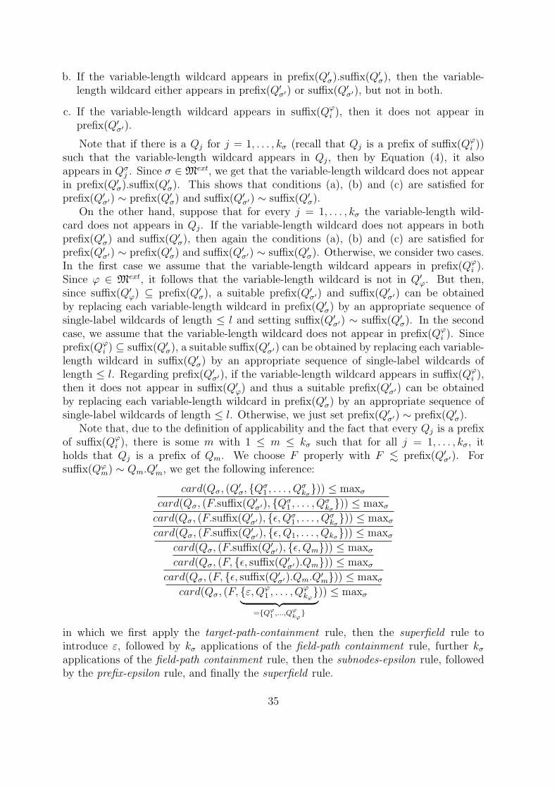
b. If the variable-length wildcard appears in prefix(Q′σ).suffix(Q′
σ), then the variable-length wildcard either appears in prefix(Q′
σ′) or suffix(Q′σ′), but not in both.
c. If the variable-length wildcard appears in suffix(Qφi ), then it does not appear in
prefix(Q′σ′).
Note that if there is a Qj for j = 1, . . . , kσ (recall that Qj is a prefix of suffix(Qφi ))
such that the variable-length wildcard appears in Qj, then by Equation (4), it alsoappears in Qσ
j . Since σ ∈ Mext, we get that the variable-length wildcard does not appearin prefix(Q′
σ).suffix(Q′σ). This shows that conditions (a), (b) and (c) are satisfied for
prefix(Q′σ′) ∼ prefix(Q′
σ) and suffix(Q′σ′) ∼ suffix(Q′
σ).On the other hand, suppose that for every j = 1, . . . , kσ the variable-length wild-
card does not appears in Qj. If the variable-length wildcard does not appears in bothprefix(Q′
σ) and suffix(Q′σ), then again the conditions (a), (b) and (c) are satisfied for
prefix(Q′σ′) ∼ prefix(Q′
σ) and suffix(Q′σ′) ∼ suffix(Q′
σ). Otherwise, we consider two cases.In the first case we assume that the variable-length wildcard appears in prefix(Qφ
i ).Since φ ∈ Mext, it follows that the variable-length wildcard is not in Q′
φ. But then,since suffix(Q′
φ) ⊆ prefix(Q′σ), a suitable prefix(Q′
σ′) and suffix(Q′σ′) can be obtained
by replacing each variable-length wildcard in prefix(Q′σ) by an appropriate sequence of
single-label wildcards of length ≤ l and setting suffix(Q′σ′) ∼ suffix(Q′
σ). In the secondcase, we assume that the variable-length wildcard does not appear in prefix(Qφ
i ). Sinceprefix(Qφ
i ) ⊆ suffix(Q′σ), a suitable suffix(Q′
σ′) can be obtained by replacing each variable-length wildcard in suffix(Q′
σ) by an appropriate sequence of single-label wildcards oflength ≤ l. Regarding prefix(Q′
σ′), if the variable-length wildcard appears in suffix(Qφi ),
then it does not appear in suffix(Q′φ) and thus a suitable prefix(Q′
σ′) can be obtainedby replacing each variable-length wildcard in prefix(Q′
σ) by an appropriate sequence ofsingle-label wildcards of length ≤ l. Otherwise, we just set prefix(Q′
σ′) ∼ prefix(Q′σ).
Note that, due to the definition of applicability and the fact that every Qj is a prefixof suffix(Qφ
i ), there is some m with 1 ≤ m ≤ kσ such that for all j = 1, . . . , kσ, itholds that Qj is a prefix of Qm. We choose F properly with F . prefix(Q′
σ′). Forsuffix(Qφ
m) ∼ Qm.Q′m, we get the following inference:
card(Qσ, (Q′σ, {Qσ
1 , . . . , Qσkσ})) ≤ maxσ
card(Qσ, (F.suffix(Q′σ′), {Qσ
1 , . . . , Qσkσ})) ≤ maxσ
card(Qσ, (F.suffix(Q′σ′), {ϵ,Qσ
1 , . . . , Qσkσ})) ≤ maxσ
card(Qσ, (F.suffix(Q′σ′), {ϵ,Q1, . . . , Qkσ})) ≤ maxσ
card(Qσ, (F.suffix(Q′σ′), {ϵ, Qm})) ≤ maxσ
card(Qσ, (F, {ϵ, suffix(Q′σ′).Qm})) ≤ maxσ
card(Qσ, (F, {ϵ, suffix(Q′σ′).Qm.Q′
m})) ≤ maxσcard(Qσ, (F, {ε,Qφ
1 , . . . , Qφkφ}︸ ︷︷ ︸
={Qφ1 ,...,Q
φkφ
}
)) ≤ maxσ
in which we first apply the target-path-containment rule, then the superfield rule tointroduce ε, followed by kσ applications of the field-path containment rule, further kσapplications of the field-path containment rule, then the subnodes-epsilon rule, followedby the prefix-epsilon rule, and finally the superfield rule.
35

The previous lemma establishes the correctness of the first assumption in the proofof Lemma 3. The second assumption in the proof of Lemma 3 holds as we can see imme-diately from applying the target-to-context rule. Finally, to verify the third assumptionwe prove the following lemma.
Lemma 5 Let Σ ∪ {φ} be a finite set of max-constraints in the class Mext, and letσ1, σ2 ∈ Σ+
R′ where σ2 = card(Qσ2 , (Q′σ2, {Qφ
1 , . . . , Qφkφ})) ≤ maxσ2. Suppose that
(wσ1 , w′σ1) witnesses the applicability of σ1 to φ where wσ1 either coincides with qφ or
is an descendant node of it in TΣ,φ, and (w′σ1, q′φ) witnesses the applicability of σ2 to φ.
Then there is a PL{., , ∗} expression Q′ and a suffix of Q′φ, denoted suffix(Q′
φ), such that
σ′ = card(Qσ1 , (Q′.suffix(Q′
φ), {Qφ1 , . . . , Q
φkφ})) ≤ maxσ1 ·maxσ2 ∈ Σ+
R′
and (wσ1 , q′φ) witnesses the applicability of σ′ to φ.
Proof Since w′σ1
is an ancestor node of q′φ and wσ1 and w′σ1
witness the applicability ofσ1 to φ, it follows that there is a suffix suffix(O′
φ) of O′φ such that suffix(O′
φ) . Q′σ2.
Since there is no sequence of single-label wildcards of length > l in σ2, we havethat suffix(Q′
φ) . Q′σ2
for Q′φ ∼ prefix(Q′
φ).suffix(Q′φ). We also have that, q′φ ∈
w′σ1[[suffix(Q′
φ)]] and, for all j = 1, . . . , kσ1 , it holds that suffix(Q′φ).suffix(Qσ1
j ) . Qσ1j
for Qσ1j ∼ prefix(Qσ1
j ).suffix(Qσ1j ). Thus, we can use kσ1 applications of the field-path
containment rule to derive the following max-constraint from σ1.
card(Qσ1 , (Q′σ1, {R})) ≤ maxσ1 ∈ Σ+
R′ (2)
where R = {suffix(Q′φ).suffix(Qσ1
1 ), . . . , suffix(Q′φ).suffix(Qσ1
kσ1)}. Note that, if there is a
variable-length wildcard in suffix(Q′φ), then there is also a variable-length wildcard in
Qσ1j for every j = 1, . . . , kσ1 and thus no variable-length wildcard can appear in Q′
σ1.
Therefore, the max-constraint in (2) is also in the class Mext.Next, we note that if the variable-length wildcard appears inQφ
i for some i = 1, . . . , kφ,then it cannot appear in Q′
φ. Otherwise φ would not be in Mext. Thus, we can replaceany variable-length wildcard that appears in Q′
σ1by an appropriate sequence of single-
label wildcards of length ≤ l. If variable-length wildcard appears in Qφi , then we set Q′
to be the the expression in PL{., } obtained by this process. Otherwise, if the variable-length wildcard does not appear in Qφ
i , we just set Q′ ∼ Q′
σ1. By applying the target-path
containment rule to (2) we get the following max-constraint which is still applicable toφ.
card(Qσ1 , (Q′, {R})) ≤ maxσ1 ∈ Σ+
R′ (3)
Then we can apply the superfield rule to obtain
card(Qσ1 , (Q′,S)) ≤ maxσ1 ∈ Σ+
R′ (4)
where S = {suffix(Q′φ).Q
φ1 , . . . , suffix(Q′
φ).Qφkφ, suffix(Q′
φ).suffix(Qσ11 ), . . . ,
suffix(Q′φ).suffix(Qσ1
kσ1)}.
36

According to applicability we have Qσ1 .Q′σ1
⊆ Qσ2 and since Q′ ⊆ Q′σ1, we also have
that Qσ1 .Q′ ⊆ Qσ2 . Recall that suffix(Q′
φ) ⊆ Q′σ2. Thus, applications of the context-
path-containment rule, the target-path-containment rule and the superfield rule to σ2
producecard(Qσ1 .Q
′, (suffix(Q′φ), T )) ≤ maxσ2 ∈ Σ+
R′ (5)
where T = {Qφ1 , . . . , Q
φkφ, suffix(Qσ1
1 ), . . . , suffix(Qσ1kσ1
)}. Note that if the variable-length
wildcard appears in suffix(Q′φ), then for every i = 1, . . . , kφ, it does not appear in Qφ
i .So, if that is the case, we assume that for every j = 1, . . . , kσ1 , there is no single-labelwildcard in Qσ1
j , since otherwise we can replace each of those variable-length wildcardsby an appropriate sequence of single-label wildcards of length ≤ l.
From (4) and (5) we infer
card(Qσ1 , (Q′.suffix(Q′
φ), T )) ≤ maxσ1 ·maxσ2 ∈ Σ+R′ (6)
by means of the multiplication rule.We now distinguish between two different cases.Case 1. Assume first that for all i = 1, . . . , kφ we have Qφ
i ∼ ε. That is, only the leafnodes of TΣ,φ are marked. It follows, by applicability of σ1 to φ, that for all j = 1, . . . , kσ1
there is some ij with 1 ≤ ij ≤ kφ such that Oφij
. Qσ1j . Thus, by construction of Oφ
ij
from Qφij, it follows that Qφ
ij. Qσ1
j , which implies that Qφij
⊆ Qσ1j . Therefore, by kσ
applications of the field-path containment rule, (6) reduces to
card(Qσ1 , (Q′.suffix(Q′
φ), {Qφ1 , . . . , Q
φkφ})) ≤ maxσ1 ·maxσ2 ∈ Σ+
R′ .
Case 2. For the remaining case we suppose that there is some l with 1 ≤ l ≤ kφ suchthat Qφ
l ∼ ε. That is, all descendant nodes of q′φ in TΣ,φ are marked. Applicability of σ1
to φ means that for all j = 1, . . . , kσ1 there is some ij with 1 ≤ ij ≤ kφ such that Oφij.
suffix(Qσ1j ).suffix(Qφ
ij). Recall that q′φ ∈ w′
σ1[[suffix(Q′
φ)]] and suffix(Q′φ).suffix(Qσ1
j ) ⊆Qσ1
j . Thus, by construction of Oφijfrom Qφ
ij, it follows that Qφ
ij⊆ suffix(Qσ1
j ).suffix(Qφij).
A repeated application of the prefix-epsilon rule to (6) results in
card(Qσ1 , (Q′.suffix(Q′
φ), T ′)) ≤ maxσ1 ·maxσ2 ∈ Σ+R′ ,
where T ′ ∼ {Qφ1 , . . . , Q
φkφ, suffix(Qσ1
1 ).suffix(Qφi1), . . . , suffix(Qσ1
kσ1).suffix(Qφ
ikσ1)}. Finally,
by repeated applications of the field-path containment rule, this reduces to
card(Qσ1 , (Q′.suffix(Q′
φ), {Qφ1 , . . . , Q
φkφ})) ≤ maxσ1 ·maxσ2 ∈ Σ+
R′ .
Hence, in both cases we derive that σ′ ∈ Σ+R′ . It is immediate that σ′ is applicable to
φ as witnessed by wσ1 and q′φ.
This concludes our proof of the assumptions made when verifying Lemma 3.
37