DECENTRALIZATION, CORRUPTION, AND POLITICAL ACCOUNTABILITY IN DEVELOPING COUNTRIES

OSKAR NUPIA*

Abstract Powerful local elites are quite common in developing countries. Thus, whether decentralization reduces or not the level of corruption in the presence of these elites is a relevant issue for these economies. We motivate this paper with some empirical evidence. Using cross-country information we find that the negative average effect of decentralization on corruption documented in the literature is absent for developing countries. Then, we build an imperfect information model of corruption and political accountability to study if the influence local elites may have on the allocation of public resources can explain this outcome. We find that not only the power of the elites but also other unexpected factors matter. In particular, both the existence of regions with a relatively weak accountability sector and the design of decentralization and grants can also explain the lack of success of decentralization in combating corruption in these economies. Keywords: Decentralization, corruption, political accountability, capture, local elites. JEL Classification: H77, D73, H72.

* I thank Antonio Cabrales, Joan Esteban, Humberto Llavador, Ernesto Stein and participants at the VII LACEA-Political Economy Network Annual Meeting for useful comments. Universidad de los Andes Department of Economics. Carrera 1 No. 18A-10, Bogotá D.C., Colombia. onupia@uniandes.edu.co.

CEDE

DOCUMENTO CEDE 2007-17 ISSN 1657-7191 (Edición Electrónica) SEPTIEMBRE DE 2007

2

DESCENTRALIZACIÓN, CORRUPCIÓN Y CONTROL POLÍTICO EN LOS PAÍSES EN VÍA DE DESARROLLO

Resumen La existencia de elites poderosas a nivel local es muy común en los países en vía de desarrollo. Saber si la descentralización reduce los niveles de corrupción cuando existen estas elites es importante para estas economías. Para motivar este artículo se presenta evidencia empírica que soporta la hipótesis de que la descentralización no posee ningún efecto sobre el nivel de corrupción en los países en vías de desarrollo. Para ver si este resultado se puede explicar por la existencia de elites locales, se construye un modelo de información asimétrica de corrupción y control político. El modelo muestra que no solo el poder de las elites locales sino otros factores inesperados son importantes para explicar este resultado. En particular, la existencia de regiones con un sector de fiscalización débil, junto con el diseño de la descentralización y las transferencias, pueden explicar la falta de existo de la descentralización para combatir la corrupción en estas economías. Palabras clave: Descentralización, corrupción, control político, captura, elites locales. Clasificación JEL: H77, D73, H72.

3

1. Introduction An important part of the literature on fiscal federalism has cared on the potential benefits decentralization may have on corruption. The main question to this respect is whether or not decentralization promotes good governance and persuades politicians against corruption. There is a partial agreement that decentralization reduces the level of corruption. This conclusion is based on both some well-known theoretical results and some of the empirical evidence available. Nevertheless, this is not the common perception in developing countries. Some authors have informally claimed that some idiosyncratic characteristics of these economies, such as the existence of powerful local elites, have not allowed decentralization to reduce the level of corruption. In this paper we study how the existence of these local elites affects the relationship between decentralization and corruption. The arguments that support the idea that decentralization reduces the level of corruption are based on at least two theories. First, jurisdictional competition discourages local governments from establishing distortionary policies that might drive away factors of production to less interventionist jurisdictions (Brenna and Buchanan, 1980; Shleifer and Vishny, 1993). Second, decentralization improves political accountability (Seabright, 1996). The idea behind this thesis is that decentralization grants the citizens of each region with the power to decide directly whether to re-elect a government or not, whereas centralization ensures that regions no longer have the same power in the re-election decision. This allows decentralization to encourage good governance. Other authors have claimed that decentralization may bring about more corruption in developing countries. The reason to think so is simple: those factors that allow decentralization to reduce corruption fail systematically in these economies. For instance, jurisdictional competition requires the existence of well-behaved common markets and that is not the rule in developing countries (Litvack et al., 1998). Furthermore, although in most of these countries popular election systems are established, powerful elites make difficult a broadly based local participation in elections (Prud’homme, 1995; Tanzi, 1995). This issue obscures political accountability through elections and makes developing countries more vulnerable to corrupt bureaucracies. The empirical evidence about the relationship between decentralization and corruption also exhibits different results. One of the most representative studies in this field is due to Fisman and Gatti (2002). They work with a cross-section of 55 (developing and developed) countries. Their results show that more decentralization implies less corruption. However, Treisman (2000, 2002) finds the opposite result by using different measures of decentralization and quality of government. To motivate our discussion, we present some suggestive evidence about the relationship between decentralization and corruption in developing countries. In order to be consistent with the available evidence, we use the same sample, data set, decentralization definition, corruption index and econometric specification used by Fisman and Gatti (2002). We show that the negative effect that fiscal decentralization has on corruption in developed countries can not be confirmed in developing economies. In the rest of the paper, we formalize the idea that the lack of success of decentralization in combating corruption in these economies can be explained by the

4

existence of powerful local elites. In doing so, we find new elements that are relevant to understand this relationship. We start by developing and analyzing an incomplete information model of corruption and political accountability in a decentralized system. We understand corruption as the use of public resources for private gains. By political accountability, we mean the capacity of citizens to detect a corrupt incumbent and remove him from office1. The game involves the voters of the jurisdiction, the respective incumbent, and a local elite that demands corruption from the office. The asymmetry in the model arises from the incumbent’s type (corrupt or non-corrupt). At election time, citizens cannot observe this type but only a signal about it. This signal is produced and sent by a local accountability sector. The accountability sector is an organized local group interested in good governance. This sector can be understood as a technology that invests all its resources in supervising the incumbent’s performance. These resources depend positively on the per capita income of the jurisdiction. We assume that the probability of detecting the incumbent in corruption increases as the resources of the accountability sector increase. In our framework, not only the accountability sector but also the elite can influence the political process by affecting the probability of detecting the incumbent in corruption. It can do it through two mechanisms. First, it can invest some resources in order to hold up the task of the accountability sector. In this way the elite reduces the probability of detection. Second, we assume the elite has economic control over a proportion of citizens. As this proportion increases, it is more difficult to detect the incumbent in corruption activities. If the incumbent is non-corrupt, then at equilibrium there is not corruption. The interesting case is that in which the incumbent is corrupt. If this is the case, we show that at equilibrium both the level of political accountability and the level of corruption are simultaneously determined by the power of the local elite, the per capita income of the jurisdiction, the incumbent’s office spoils, and the incumbent’s share in corruption – i.e. the proportion that incumbent reserves to himself from the resources allocated in corruption. To model the centralized case, we use the same framework described above. The novelty is that, under centralization, there is a local elite in each jurisdiction demanding corruption not to a local incumbent but to a central bureaucrat. This extension does not affect the equilibrium representation of the model. Thus, both the level of corruption and political accountability under centralization depend on the total power of the local elites at the national (federal) level, the national per capita income of the federation, the federal incumbent’s office spoils, and the federal incumbent’s share in corruption. Our aim is to study how corruption and political accountability change when a federation moves from a centralized to a decentralized system. We do so by analysing how the parameters of the model change between the federal (national) level and the jurisdictional level. We start by comparing the power of the elites at the national level against the power of the elite at the jurisdictional level. Our model predicts that, if the latter is larger than the former, then decentralization increases (reduces) the level of

1 It is important to note that this concept differs from the Seabright’s definition of accountability, which refers to the probability that the welfare of a region can determine the re-election of the government.

5

corruption (political accountability). The opposite happens if the latter is smaller than the former. The final effect of decentralization (via the elites' power) on national corruption and accountability is difficult to predict. It depends on the distribution of these powers across the jurisdictions and the initial level of corruption. The second relevant comparison is between the national and the jurisdictional per capita income. We show that, if the jurisdictional per capita income is larger than the federal per capita income, decentralization reduces (increases) the level of corruption (political accountability) if and only if the resources of the accountability sector grow above the locally generated taxes. Otherwise, decentralization increases (reduces) the level of corruption (political accountability). An analogous result is obtained if the jurisdictional per capita income is smaller than the national per capita income. Once again, the final effect of decentralization (via per capita income) on corruption and political accountability is ambiguous. It depends on the dispersion of income across the jurisdictions. Nevertheless, it is not hard to think that corruption (political accountability) will increase (decrease) in many jurisdictions in developing countries, which usually are characterized by a relative weak accountability sector. An important corollary of this result has to do with the use of grants or transfers from the central government to the jurisdictions. Grants affect the amount of resources that an incumbent can allocate in his jurisdiction positively, but do not affect the amount of resources that the accountability sector has to invest on political accountability. When this happens, our model predicts an increment (reduction) in the level of corruption (political accountability). This is an important issue for developing countries, where the central governments use transfers intensively in order to reduce the high between-jurisdiction income inequality. The third relevant element is the office spoils. National office spoils are expected to be larger than jurisdictional office spoils, independently of the level of development. Our model predicts that under these circumstances, decentralization increases the level of corruption. Nevertheless, the effect on political accountability is ambiguous. Thus, the decentralization design also affects the level of corruption. For instance, the office spoils in small municipalities are farther from the national ones than the respective spoils in states. Therefore, when a federation is decentralized, corruption will increase more if it focuses on small jurisdictions than if it does on states. Decentralization in developing countries has allocated many tasks to small municipalities. The last key element is the incumbent’s share in corruption. Some authors (e.g. Tanzi, 1995) have claimed that rewards to local politicians are relatively smaller than those received by central bureaucrats. Our model predicts that when this is the case and this share is not too high, decentralization reduces the level of corruption. However, the effect on accountability is ambiguous. The final effect of decentralization on the nationwide level of corruption and political accountability depends on the combination of all the factors mentioned above. Thus, it is difficult to make a clear prediction about this effect. Nevertheless, our empirical evidence suggests that decentralization has not affected the level of corruption in developing countries. This outcome can be explained by the interaction of the parameters in our model. How local elites affect the relationship between corruption and decentralization has not been formally studied in the literature. The paper by Bardhan and Mookherjee (2000) is quite close to this issue. They investigate the determinants of relative capture of local

6

and national governments. However, in their model capture is produced on the political position of the government with respect to a public policy. Our model is more specific in terms of corruption. Here, elites do not influence explicitly the position of the government in a public policy but influence the allocation of public resources between public goods and corruption. The rest of the paper is organized as follows. Section 2 presents the empirical motivation. Section 3 develops the decentralized framework, and section 4 analyses its comparative statics. Section 5 extents the model to the case of centralization, and section 6 studies how both the level of corruption and political accountability change when a federation is decentralized. Section 7 concludes. The appendix contains all proofs. 2. Empirical Motivation As we have already mentioned, one of the most representative empirical studies in this field supports the hypothesis that decentralization reduces corruption. However, whether or not the dissuasive effect of decentralization on corruption is systematically present in both developing and developed countries is an unexplored issue. In order to motivate our discussion, in this section we present some empirical evidence on that. To be consistent with the available evidence, we are going to use the same sample, data set, corruption indicator, and definition of decentralization used by Fisman and Gatti (2002) (hereafter F&G). The decentralization index corresponds to the ratio between the total expenditure of subnational (state and local) governments and the total spending by all government levels (state, local, and central). Correspondingly, the measure of corruption is the International Country Risk Guide (ICRG) corruption index. This index has been rescaled such that it lies between 0 and 1, where 0 indicates least corruption.

We also work with the same basic econometric specification used by F&G, which assumes that corruption is a function of fiscal decentralization, per capita income, population, public sector’s size, and civil liberties. All the variables are averages for the period 1980-1995, except population which corresponds to a geometric average. The exact definition of the complete set of variables is given in the appendix.2 In order to test our hypothesis, we allow for a different effect of decentralization in developed and developing countries. The results are reported in table 1. All the standard deviations of the parameters are robustly estimated.

2 There are three differences between the F&G’s data set and the one used here: (1) Population is taken from Heston, Summers and Aten, Penn World Table Version 6.1, whereas F&G’s source is World Development Bank Indicators. (2) For government size (total government expenditure divided by GDP) F&G use Barro (1991)’s information. When we use this source the country sample is reduced in a high proportion, and it does not coincide with the F&G’s sample. Thus, we use government size from Heston et al., which additionally includes information for the whole period 1980-1995. (3) The GDP information used by F&G is in 1985 price, and the one used here is 1996 price.

7

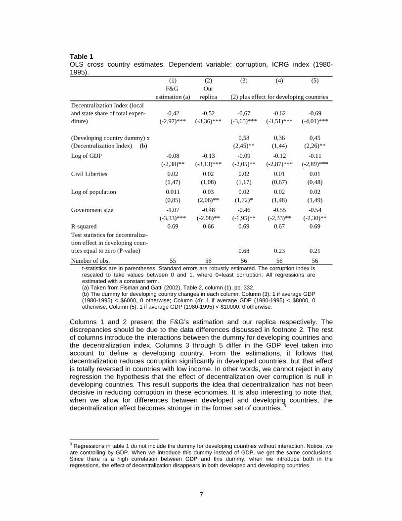
Table 1 OLS cross country estimates. Dependent variable: corruption, ICRG index (1980-1995).

(1) (2) (3) (4) (5)F&G Our

estimation (a) replicaDecentralization Index (local and state share of total expen-diture)

-0,42 (-2,97)***

-0,52 (-3,36)***

-0,67 (-3,65)***

-0,62 (-3,51)***

-0,69 (-4,01)***

(Developing country dummy) x (Decentralization Index) (b)

0,58 (2,45)**

0,36 (1,44)

0,45 (2,26)**

Log of GDP -0.08 -0.13 -0.09 -0.12 -0.11(-2,38)** (-3,13)*** (-2,05)** (-2,87)*** (-2,89)***

Civil Liberties 0.02 0.02 0.02 0.01 0.01(1,47) (1,08) (1,17) (0,67) (0,48)

Log of population 0.011 0.03 0.02 0.02 0.02(0,85) (2,06)** (1,72)* (1,48) (1,49)

Government size -1.07 -0.48 -0.46 -0.55 -0.54(-3,33)*** (-2,08)** (-1,95)** (-2,33)** (-2,30)**

R-squared 0.69 0.66 0.69 0.67 0.69Test statistics for decentraliza-tion effect in developing coun-tries equal to zero (P-value) 0.68 0.23 0.21Number of obs. 55 56 56 56 56

(2) plus effect for developing countries

t-statistics are in parentheses. Standard errors are robustly estimated. The corruption index is rescaled to take values between 0 and 1, where 0=least corruption. All regressions are estimated with a constant term. (a) Taken from Fisman and Gatti (2002), Table 2, column (1), pp. 332. (b) The dummy for developing country changes in each column. Column (3): 1 if average GDP (1980-1995) < $6000, 0 otherwise; Column (4): 1 if average GDP (1980-1995) < $8000, 0 otherwise; Column (5): 1 if average GDP (1980-1995) < $10000, 0 otherwise.

Columns 1 and 2 present the F&G’s estimation and our replica respectively. The discrepancies should be due to the data differences discussed in footnote 2. The rest of columns introduce the interactions between the dummy for developing countries and the decentralization index. Columns 3 through 5 differ in the GDP level taken into account to define a developing country. From the estimations, it follows that decentralization reduces corruption significantly in developed countries, but that effect is totally reversed in countries with low income. In other words, we cannot reject in any regression the hypothesis that the effect of decentralization over corruption is null in developing countries. This result supports the idea that decentralization has not been decisive in reducing corruption in these economies. It is also interesting to note that, when we allow for differences between developed and developing countries, the decentralization effect becomes stronger in the former set of countries. 3

3 Regressions in table 1 do not include the dummy for developing countries without interaction. Notice, we are controlling by GDP. When we introduce this dummy instead of GDP, we get the same conclusions. Since there is a high correlation between GDP and this dummy, when we introduce both in the regressions, the effect of decentralization disappears in both developed and developing countries.

8

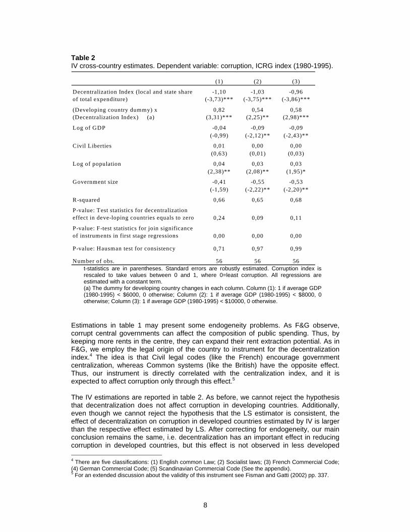
Table 2 IV cross-country estimates. Dependent variable: corruption, ICRG index (1980-1995).

t-statistics are in parentheses. Standard errors are robustly estimated. Corruption index is rescaled to take values between 0 and 1, where 0=least corruption. All regressions are estimated with a constant term. (a) The dummy for developing country changes in each column. Column (1): 1 if average GDP (1980-1995) < $6000, 0 otherwise; Column (2): 1 if average GDP (1980-1995) < $8000, 0 otherwise; Column (3): 1 if average GDP (1980-1995) < $10000, 0 otherwise.

Estimations in table 1 may present some endogeneity problems. As F&G observe, corrupt central governments can affect the composition of public spending. Thus, by keeping more rents in the centre, they can expand their rent extraction potential. As in F&G, we employ the legal origin of the country to instrument for the decentralization index.4 The idea is that Civil legal codes (like the French) encourage government centralization, whereas Common systems (like the British) have the opposite effect. Thus, our instrument is directly correlated with the centralization index, and it is expected to affect corruption only through this effect.5 The IV estimations are reported in table 2. As before, we cannot reject the hypothesis that decentralization does not affect corruption in developing countries. Additionally, even though we cannot reject the hypothesis that the LS estimator is consistent, the effect of decentralization on corruption in developed countries estimated by IV is larger than the respective effect estimated by LS. After correcting for endogeneity, our main conclusion remains the same, i.e. decentralization has an important effect in reducing corruption in developed countries, but this effect is not observed in less developed 4 There are five classifications: (1) English common Law; (2) Socialist laws; (3) French Commercial Code; (4) German Commercial Code; (5) Scandinavian Commercial Code (See the appendix). 5 For an extended discussion about the validity of this instrument see Fisman and Gatti (2002) pp. 337.

(1) (2) (3)

Decentralization Index (local and state share of total expenditure)

-1,10 (-3,73)***

-1,03 (-3,75)***

-0,96 (-3,86)***

(Developing country dummy) x (Decentralization Index) (a)

0,82 (3,31)***

0,54 (2,25)**

0,58 (2,98)***

Log of GDP -0,04 -0,09 -0,09(-0,99) (-2,12)** (-2,43)**

Civil Liberties 0,01 0,00 0,00(0,63) (0,01) (0,03)

Log of population 0,04 0,03 0,03(2,38)** (2,08)** (1,95)*

Government size -0,41 -0,55 -0,53(-1,59) (-2,22)** (-2,20)**

R-squared 0,66 0,65 0,68

P-value: Test statistics for decentralization effect in deve-loping countries equals to zero 0,24 0,09 0,11

P-value: F-test statistics for join significance of instruments in first stage regressions 0,00 0,00 0,00

P-value: Hausman test for consistency 0,71 0,97 0,99

Number of obs. 56 56 56

9

economies. How can this outcome be explained? We care on this issue in the rest of the paper. 3. The Decentralized Federation We start by analysing an incomplete information model of political accountability and corruption in a single jurisdiction, i.e. when the federation is totally decentralized. The game is played by the jurisdiction’s voters, their respective incumbent and one local elite. There is also an organized local group interested in good governance that is called the accountability sector. This sector is not a formal player in the game, but just an information technology. In the game, the local elite demands corruption from the incumbent (in form of public resources) in order to obtain private gains. The resources allocated by the incumbent in this activity are identified as corruption. Incumbent At the beginning of the game, there is an incumbent who is (exogenously) in office. This incumbent has an amount of resources τ(y) that should be invested in a public good z but might go to corruption r. τ are the locally generated taxes, which are assumed to be a positive function of the regional income y (i.e. 0' >τ ). The unit price of the public good is normalized to be one. Thus, the incumbent budget constraint is

rz +=τ . All these variables are measured in per capita terms. The incumbent can be of two types t ∈ {c,n}, where c stands for corrupt and n for non-corrupt, with γ== )ntPr( . An incumbent of type n receives an infinitely negative utility from corruption; thus, he will always reject any corruption demand. An incumbent of type c receives a linear positive utility from corruption. For any unit of resources that he allocates to corruption to serve the elite’s demand, he will ask for himself an exogenous share β ∈ (0,1). We shall refer to β as the incumbent’s share. It can be understood as the incumbent’s share arising from a bargaining game between the incumbent and the elite. Thus, when incumbent accepts a level of corruption r, he will receive βr units of utility. The remaining (1-β)r will go to the elite. No matter his type, an incumbent gets spoils (“ego-rents”) S>0 if he stays in office. Accountability sector In our framework, political accountability is understood as the capacity of citizens to detect the incumbent in corruption and to remove him from the office. In the model there is an accountability sector that cares on improving political accountability in order to encourage good governance. You can think this sector is formed by civic associations, independent (non-influenced) media, and central government’s control offices. This sector is endowed with an amount of resources A that is totally invested in supervising the incumbent’s performance. These resources are also measured in per capita terms. We allow these resources to depend positively on the per capita jurisdiction’s income (y), then A=A(y) with 0'A > . The main task of the accountability sector is to send a signal to the citizens announcing whether the incumbent is corrupt or not. This sector can be understood as a technology that invests all its resources into accountability and makes an announcement about the incumbent’s type. In particular, it is not a formal player. We assume this sector is not

10

influenced by any player in the game; thus, it will only transmit true information to the voters. Voters Let )z(u be the utility that voters receive from the public good supplied by the incumbent, with u strictly increasing. An incumbent of type n will provide a utility )(u τ to the voters, whereas an incumbent of type c will deliver )r(u −τ . After observing the outcome, voters must decide whether they re-elect the incumbent or randomly elect a candidate from the opposition whose type will be n with probability γ. Nevertheless, we assume that voters are not able to observe their payoff directly at the time of elections but only a signal from the accountability sector. If the incumbent’s type is n, the accountability sector will receive and send a signal s=n. However, if the incumbent is corrupt, it will receive and send a signal s=c with probability δ ∈ [0,1], and s=n with probability 1-δ. Whit this information, the citizens vote in order to maximize their expected utility. The probability of detecting the incumbent in corruption (δ) will be established endogenously in the model. We will define it formally later on. Elite The elite demands corruption r from the jurisdiction’s incumbent in order to produce some personal benefits. One can think in some specific project that affects the benefits on the elite directly and positively: licenses, public contracts, market interventions, etc.6 When the incumbent accepts the corruption demand, the elite receives the fraction 1-β of r. With this amount of resources, it is going to produce ( )r)1(Q β− benefits, where

0'Q > . We assume that the elite can influence the political process by affecting the probability of detecting the incumbent in corruption (δ). It can do it through two mechanisms. First, it can invest some resources H in order to hold up the task of the accountability sector. In this way the elite reduces δ. For instance, these resources may be spent on bribing other involved public workers, falsifying some documents, altering the account books, and so on. Second, the elite has economic control over a proportion θ ∈ [0,1/2) of citizens, which makes it more difficult to detect the incumbent in corruption activities. One can think that the elite has some monopsonistic power in the jurisdiction’s labor market and so it can induce these people to cover any signal of corruption. If this is the case, the resources invested by the accountability sector will be less productive as θ increases. We refer to θ as the elite’s power. To simplify, we assume the elite does not face any cost when it demands corruption to the incumbent. This implies that, if the incumbent’s type is n, the elite will not face any penalty if it insinuates a corruption agreement to the former. Assuming a linear Q(.), the elite’s expected payoff will be ( )( )Hr)1(1 −−−= βγπ .

6 Notice that in some of these cases corruption may also affect the citizens’ welfare positively. However, since our analysis is not about welfare but about corruption, we do not care on these external effects.

11

Detection probability and accountability level Up to now there are three variables affecting the detection probability (δ): A, which is a function of y and has a positive effect on it; and H and θ, which affect δ negatively. In Addition to these three effects, we shall allow for a moral hazard component. This component takes into account the fact that the more rent is allocated to corruption as a proportion of the local taxes, the easier it is for the accountability sector to find out about corruption. To simplify the algebra, while preserving sufficient richness of structure, we will assume:

( ) ( )τΨθδ rHA

A1+

−= (1)

where 0)0( =Ψ , 1)1( =Ψ , 0(.)' >Ψ , 0(.)'' >Ψ , ∞<)0('Ψ , 0)0('' =Ψ , and

∞=→

(.)'limr

Ψτ

. The four first assumptions ensure Ψ belongs to the interval [0,1], and

both the moral hazard probability and its marginal rate strictly increase in τr . The remaining are technical assumptions. Keep in mind that τ is a function of y, so ultimately Ψ(.) is also a function of y. We call this component the moral hazard probability.7 As we mentioned earlier, political accountability in our framework is understood as the ability of citizens to detect the incumbent in corruption and remove her from office. One can be tempted to relate this concept directly to the detection probability. However, δ may not represent this concept accurately because of the moral hazard component. Consider the following situation. Imagine there is a variable that affects the level of corruption negatively and so (.)Ψ , but, at the same time, it affects ( )( ))HA(A1 +−θ (the other part of δ) positively. When the first effect dominates the second effect, the final result is a reduction in δ.8 If we do not make any distinction between the level of accountability and the detection probability, we conclude that the former also decreases. However, since in the new situation either elite has less influence on δ (via H or θ) or the accountability sector is more effective or both, this conclusion is not right at all. Thus, in order to measure the degree of political accountability (δa), we remove the moral hazard probability from δ:

( )HA

A1a +−= θδ (2)

7 Notice that if τ=r , ( ) ( ) 1HAA1 <+−= θδ . However, although δ is not equals one when the incumbent spends the total amount of taxes in corruption, this functional form allows us to obtain an interior solutions for the level of corruption. We could use equation 1 to define δ if τ<r and set 1=δ if

τ=r . It does not add any new to our results. 8 As we shall see later on, the situation described in this example always holds.

12

Game and Equilibrium In order to keep the framework as simple as possible, we assume that an incumbent type c does not extract rents without the elite participation. This allows us to concentrate on the corruption generated from the elite intervention. With the accountability group investing A in accountability, the timing of the game is as follows: Stage 1: Elite offers a contract r,H to the incumbent. Stage 2: The incumbent decides whether to accept (Y) or reject (N) the contract. Stage 3: Citizens observe the accountability sector signal and vote for the candidate (the incumbent or another candidate of unknown type) that maximizes their expected utility. The equilibrium of the game has two components. The first one is the game between the elite and the incumbent, which determines the levels of both corruption and political accountability. The second is the equilibrium in the election game, which establishes whether the incumbent is re-elected or not. To model the equilibrium in the corruption market, we focus on perfect Bayesian equilibrium restricted to pure-strategy equilibria in which citizens always vote for their preferred candidate. The complete description of the equilibrium strategies and proofs of the following propositions can be found in the appendix. Here, we state the equilibrium conditions when there is a positive level of corruption. We now introduce subscript j to denote jurisdictions and superscript d to denote outcomes and parameters under decentralization. Proposition 1. When incumbent is of type c, at equilibrium the incumbent always accepts the contract (with positive corruption) offered by the elite. The equilibrium contract d

jdj r,H satisfies the following conditions:

( )⎟⎟⎟

⎠

⎞

⎜⎜⎜

⎝

⎛ −−=− 2d

j

dj

d

ddjd

r

(.)(.)r(.)'S(.)A1)1(

ΨτΨ

β

θβ (3)

⎟⎟

⎠

⎞

⎜⎜

⎝

⎛−

−= 1S

r(.))1(

(.)AH ddj

d

djd

jΨ

β

θ (4)

where ( ).A and ( ).τ depend on jy , and ( ).Ψ is evaluated at ( ).r d

j τ . Equation 3

implicitly sets the equilibrium level of corruption in jurisdiction j ( djr ) under

decentralization. This happens at the point in which the elite’s marginal income of corruption ( )d1 β− equals the elite’s marginal cost of corruption. Equation 4 sets the

minimum level of djH required by the incumbent to accept d

jr . At equilibrium, the public good supply, the accountability level, and the detection probability are given respectively by:

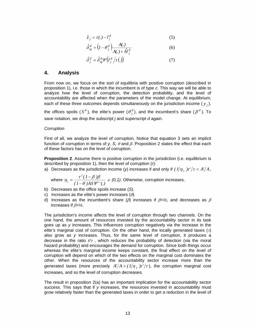
13

djj r(.)z −= τ (5)

( ) dj

dj

daj H(.)A

(.)A1ˆ+

−= θδ (6)

( )( ).rˆˆ dj

daj

dj τΨδδ = (7)

4. Analysis From now on, we focus on the sort of equilibria with positive corruption (described in proposition 1), i.e. those in which the incumbent is of type c. This way we will be able to analyze how the level of corruption, the detection probability, and the level of accountability are affected when the parameters of the model change. At equilibrium, each of these three outcomes depends simultaneously on the jurisdiction income ( jy ),

the offices spoils ( dS ), the elite’s power ( djθ ), and the incumbent’s share ( dβ ). To

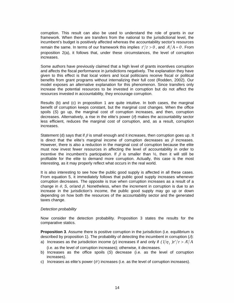
save notation, we drop the subscript j and superscript d again. Corruption First of all, we analyze the level of corruption. Notice that equation 3 sets an implicit function of corruption in terms of y, S, θ and β. Proposition 2 states the effect that each of these factors has on the level of corruption. Proposition 2. Assume there is positive corruption in the jurisdiction (i.e. equilibrium is described by proposition 1), then the level of corruption (r): a) Decreases as the jurisdiction income (y) increases if and only if A'A')1( 1 <ττη ,

where (.)''AS)1(

)1(2

1 Ψθββτη

−−

= ∈ (0,1). Otherwise, corruption increases.

b) Decreases as the office spoils increase (S). c) Increases as the elite’s power increases (θ). d) Increases as the incumbent’s share (β) increases if β<½, and decreases as β

increases if β>½. The jurisdiction’s income affects the level of corruption through two channels. On the one hand, the amount of resources invested by the accountability sector in its task goes up as y increases. This influences corruption negatively via the increase in the elite’s marginal cost of corruption. On the other hand, the locally generated taxes (τ) also grow as y increases. Thus, for the same level of corruption, it produces a decrease in the ratio r/τ , which reduces the probability of detection (via the moral hazard probability) and encourages the demand for corruption. Since both things occur whereas the elite’s marginal income keeps constant, the final effect on the level of corruption will depend on which of the two effects on the marginal cost dominates the other. When the resources of the accountability sector increase more than the generated taxes (more precisely ττη ')1(A'A 1> ), the corruption marginal cost increases, and so the level of corruption decreases. The result in proposition 2(a) has an important implication for the accountability sector success. This says that if y increases, the resources invested in accountability must grow relatively faster than the generated taxes in order to get a reduction in the level of

14

corruption. This result can also be used to understand the role of grants in our framework. When there are transfers from the national to the jurisdictional level, the incumbent’s budget is positively affected whereas the accountability sector’s resources remain the same. In terms of our framework this implies 0' >ττ , and 0A'A = . From proposition 2(a), it follows that, under these circumstances, the level of corruption increases. Some authors have previously claimed that a high level of grants incentives corruption and affects the fiscal performance in jurisdictions negatively. The explanation they have given to this effect is that local voters and local politicians receive fiscal or political benefits from grant programs without internalizing their full cost (Rodden, 2002). Our model exposes an alternative explanation for this phenomenon. Since transfers only increase the potential resources to be invested in corruption but do not affect the resources invested in accountability, they encourage corruption. Results (b) and (c) in proposition 1 are quite intuitive. In both cases, the marginal benefit of corruption keeps constant, but the marginal cost changes. When the office spoils (S) go up, the marginal cost of corruption increases, and then, corruption decreases. Alternatively, a rise in the elite’s power (θ) makes the accountability sector less efficient, reduces the marginal cost of corruption, and, as a result, corruption increases. Statement (d) says that if β is small enough and it increases, then corruption goes up. It is direct that the elite’s marginal income of corruption decreases as β increases. However, there is also a reduction in the marginal cost of corruption because the elite must now invest fewer resources in affecting the level of accountability in order to incentive the incumbent’s participation. If β is smaller than ½, then it will still be profitable for the elite to demand more corruption. Actually, this case is the most interesting, as it may properly reflect what occurs in the real world. It is also interesting to see how the public good supply is affected in all these cases. From equation 5, it immediately follows that public good supply increases whenever corruption decreases. The opposite is true when corruption increases as a result of a change in θ, S, or/and β. Nonetheless, when the increment in corruption is due to an increase in the jurisdiction’s income, the public good supply may go up or down depending on how both the resources of the accountability sector and the generated taxes change. Detection probability Now consider the detection probability. Proposition 3 states the results for the comparative statics. Proposition 3. Assume there is positive corruption in the jurisdiction (i.e. equilibrium is described by proposition 1). The probability of detecting the incumbent in corruption (δ): a) Increases as the jurisdiction income (y) increases if and only if A'A')1( 1 >ττη

(i.e. as the level of corruption increases); otherwise, it decreases. b) Increases as the office spoils (S) decrease (i.e. as the level of corruption

increases). c) Increases as elite’s power (θ ) increases (i.e. as the level of corruption increases).

15

d) Increases as the incumbent’s share (β) increases if and only if )21( ββΦ −−> ,

where 0)1(2(.)'')1( 2 >−−Ψ−=Φ ββτ

θ AS. Notice that if β<½, this condition

always holds (i.e. it increases as the level of corruption increases). We must be careful in the interpretation of results in proposition 3. Essentially, all these results say that the detection probability increases whenever the level of corruption increases and vice versa. This is so because the moral hazard component always dominates the total effect over the detection probability. Thus, when r increases the moral hazard component goes up and so the detection probability9. A direct way to see that the moral hazard probability dominates the final effect on δ is through the incumbent’s participation constraint. At equilibrium, this constraint implies

Srˆ βδ = (See proof of proposition 3). Hence, keeping β and S constant, the detection probability increases whenever the level of corruption increases. When the changes in corruption stem from a variation in S, the final effect is strengthened by it. When it stems from a variation in β, the final effect will depend, among other things, on the value of β (as it is described in proposition 3(d)). Thus, as we have already discussed in section 3, it is better if we focus on an appropriate measure of political accountability. By doing so, we can see whether or not the voters are able to detect a corrupt incumbent not via the level of corruption but via the efficiency of the accountability sector. Political Accountability Equation 2 shows that besides the direct effect of θ and y, the accountability level depends crucially on the elite’s investment H. The comparative statics’ results are stated in proposition 4. Proposition 4. Assume there is positive corruption in the jurisdiction (i.e. equilibrium is described by proposition 1). The level of political accountability (δa): a) Increases as the jurisdiction income (y) increases if and only if

A'A')1( 21 <− ττηη , where 01r)1(.)('' 1

2 >−

=η

τββΨ

Φη . Otherwise, it

decreases. b) Can increase or decrease as the office spoils (S) increase. Only when the effect of

S over r is large enough it increases. c) Decreases as the elite’s power (θ) increases. d) Increases as the incumbent’s share (β) increases if β>½. If β<½, it increases only if

the effect of β over r is small enough. Statement (a) says that when the jurisdiction’s income increases, the resources of the accountability sector must grow at least 211 ηη − times the locally generated taxes in order to observe an increment in accountability. We cannot infer the sign of 211 ηη −

9 This assertion is true when the rise in r is not due to an increment in y (if so, unambiguously r/τ increases). However, when r increases as a result of an increment in y, the ratio r/τ does not necessarily increase, and the final effect on the moral hazard probability is ambiguous. As proposition 3 shows, even in this case, the total effect on δ is also dominated by the change in r.

16

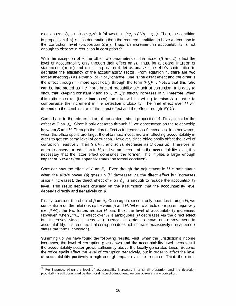
(see appendix), but since η2>0, it follows that )1(1 211 ηηη −> . Then, the condition in proposition 4(a) is less demanding than the required condition to have a decrease in the corruption level (proposition 2(a)). Thus, an increment in accountability is not enough to observe a reduction in corruption.10 With the exception of θ, the other two parameters of the model (S and β) affect the level of accountability only through their effect on H. Thus, for a clearer intuition of statements (b), (c) and (d) in proposition 4, let us analyze the elite’s contribution to decrease the efficiency of the accountability sector. From equation 4, there are two forces affecting H as either S, or θ, or β change. One is the direct effect and the other is the effect through r - more specifically through the term r(.)Ψ . Notice that this ratio can be interpreted as the moral hazard probability per unit of corruption. It is easy to show that, keeping constant y and so τ, r(.)Ψ strictly increases in r. Therefore, when this ratio goes up (i.e. r increases) the elite will be willing to raise H in order to compensate the increment in the detection probability. The final effect over H will depend on the combination of the direct effect and the effect through r(.)Ψ . Come back to the interpretation of the statements in proposition 4. First, consider the effect of S on aδ . Since it only operates through H, we concentrate on the relationship between S and H. Through the direct effect H increases as S increases. In other words, when the office spoils are large, the elite must invest more in affecting accountability in order to get the same level of corruption. However, since office spoils affect the level of corruption negatively, then r(.)Ψ , and so H, decrease as S goes up. Therefore, in order to observe a reduction in H, and so an increment in the accountability level, it is necessary that the latter effect dominates the former. This implies a large enough impact of S over r (the appendix states the formal condition). Consider now the effect of θ on aδ . Even though the adjustment in H is ambiguous when the elite’s power (θ) goes up (H decreases via the direct effect but increases since r increases), the direct effect of θ on aδ is enough to reduce the accountability level. This result depends crucially on the assumption that the accountability level depends directly and negatively on θ. Finally, consider the effect of β on δa. Once again, since it only operates through H, we concentrate on the relationship between β and H. When β affects corruption negatively (i.e. β>½), the two forces reduce H, and thus, the level of accountability increases. However, when β<½, its effect over H is ambiguous (H decreases via the direct effect but increases since r increases). Hence, in order to have an improvement in accountability, it is required that corruption does not increase excessively (the appendix states the formal condition). Summing up, we have found the following results. First, when the jurisdiction’s income increases, the level of corruption goes down and the accountability level increases if the accountability sector grows sufficiently above the locally generated taxes. Second, the office spoils affect the level of corruption negatively, but in order to affect the level of accountability positively a high enough impact over it is required. Third, the elite’s

10 For instance, when the level of accountability increases in a small proportion and the detection probability is still dominated by the moral hazard component, we can observe more corruption.

17

power affects corruption positively and the accountability level negatively. Finally, when β<½ - which actually is the most interesting case - an increment in the incumbent’s share increases the level of corruption but has an ambiguous effect on political accountability. 5. The Centralized Federation So far, the model presented in section 3 describes how both corruption and political accountability are determined in each jurisdiction in a decentralized federation. In this section we consider the case in which the federation is totally centralized. In order to do so, we use exactly the same framework we introduced in section 3. The main difference is that under centralization there is only one central incumbent in the federation who receives corruption demands from J>1 elites, one in each jurisdiction (where J is the number of jurisdictions). From now on, we use superscript c to denote parameters and outcomes under centralization. There are some issues we must take into account in this new framework. First, we are characterizing the national per capita level of corruption cr , i.e. the amount of resources allocated in corruption as proportion of the total population in the federation.

In particular, ∑ == J

1jcj

c rr , where cjr is the amount of resources allocated in

corruption in each jurisdiction j under centralization as proportion of the total population

in the federation. ∑ == J

1jcj

c HH , is defined in a similar way.

Second, under centralization the relevant parameters are those at the federal level. For instance, the power of the elites is their total power at the federal level. We define c

jθ as the percentage of people that elite j controls in its jurisdiction as proportion of the federal population. Thus, the total power of the elites at the federal level is

∑ == J

1jcj

c θθ . The other relevant parameters are the national (federal) per capita

income cy , the central (federal) office spoils cS , and the central incumbent’s share in

corruption cβ . Keeping in mind these changes, we define the probability of detecting the central incumbent in a corruption agreement with the elites in the following way:

( ) ( )( )

( )( ).rH.A

.A1 cc

cc τΨθδ+

−= (8)

where ( ).A and ( ).τ depend on cy . The last issue has to do with the accountability sector. When the system moves from centralization to decentralization, we are implicitly assuming that the accountability sector is decentralized at the same time. In other words, we are imposing that under centralization there is one national accountability sector which supervises the central incumbent, whereas under decentralization there is one group in each jurisdiction carrying out this task. In order to avoid any extra effect, we keep the characteristics of

18

the accountability sector unchanged at the two levels, i.e. both the jurisdictional and the national sector use the same technology11. The timing of the game is similar to that in the decentralization case: Stage 1: Each elite j simultaneously offers a contract c

jcj r,H to the central

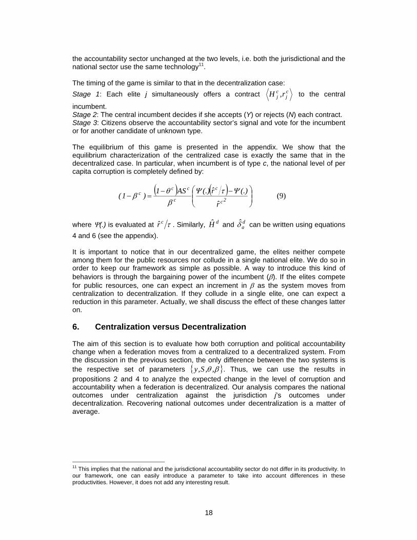
incumbent. Stage 2: The central incumbent decides if she accepts (Y) or rejects (N) each contract. Stage 3: Citizens observe the accountability sector’s signal and vote for the incumbent or for another candidate of unknown type. The equilibrium of this game is presented in the appendix. We show that the equilibrium characterization of the centralized case is exactly the same that in the decentralized case. In particular, when incumbent is of type c, the national level of per capita corruption is completely defined by:

( ) ( )⎟⎟⎠

⎞⎜⎜⎝

⎛ −−=− 2c

c

c

ccc

r

(.)r(.)AS1)1( ΨτΨβθβ (9)

where Ψ(.) is evaluated at τcr . Similarly, dH and d

aδ can be written using equations 4 and 6 (see the appendix). It is important to notice that in our decentralized game, the elites neither compete among them for the public resources nor collude in a single national elite. We do so in order to keep our framework as simple as possible. A way to introduce this kind of behaviors is through the bargaining power of the incumbent (β). If the elites compete for public resources, one can expect an increment in β as the system moves from centralization to decentralization. If they collude in a single elite, one can expect a reduction in this parameter. Actually, we shall discuss the effect of these changes latter on. 6. Centralization versus Decentralization The aim of this section is to evaluate how both corruption and political accountability change when a federation moves from a centralized to a decentralized system. From the discussion in the previous section, the only difference between the two systems is the respective set of parameters { }βθ ,,S,y . Thus, we can use the results in propositions 2 and 4 to analyze the expected change in the level of corruption and accountability when a federation is decentralized. Our analysis compares the national outcomes under centralization against the jurisdiction j’s outcomes under decentralization. Recovering national outcomes under decentralization is a matter of average. 11 This implies that the national and the jurisdictional accountability sector do not differ in its productivity. In our framework, one can easily introduce a parameter to take into account differences in these productivities. However, it does not add any interesting result.

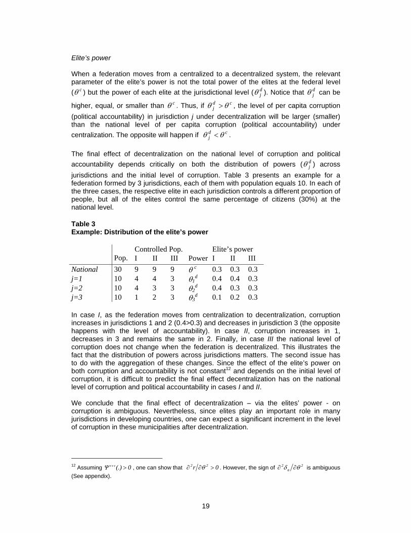
19

Elite’s power When a federation moves from a centralized to a decentralized system, the relevant parameter of the elite’s power is not the total power of the elites at the federal level ( cθ ) but the power of each elite at the jurisdictional level ( d

jθ ). Notice that djθ can be

higher, equal, or smaller than cθ . Thus, if cdj θθ > , the level of per capita corruption

(political accountability) in jurisdiction j under decentralization will be larger (smaller) than the national level of per capita corruption (political accountability) under centralization. The opposite will happen if cd

j θθ < . The final effect of decentralization on the national level of corruption and political accountability depends critically on both the distribution of powers ( d

jθ ) across jurisdictions and the initial level of corruption. Table 3 presents an example for a federation formed by 3 jurisdictions, each of them with population equals 10. In each of the three cases, the respective elite in each jurisdiction controls a different proportion of people, but all of the elites control the same percentage of citizens (30%) at the national level.

Table 3 Example: Distribution of the elite’s power Controlled Pop. Elite’s power

Pop. I II III Power I II III

National 30 9 9 9 θ c 0.3 0.3 0.3 j=1 10 4 4 3 θ1

d 0.4 0.4 0.3 j=2 10 4 3 3 θ2

d 0.4 0.3 0.3 j=3 10 1 2 3 θ3

d 0.1 0.2 0.3 In case I, as the federation moves from centralization to decentralization, corruption increases in jurisdictions 1 and 2 (0.4>0.3) and decreases in jurisdiction 3 (the opposite happens with the level of accountability). In case II, corruption increases in 1, decreases in 3 and remains the same in 2. Finally, in case III the national level of corruption does not change when the federation is decentralized. This illustrates the fact that the distribution of powers across jurisdictions matters. The second issue has to do with the aggregation of these changes. Since the effect of the elite’s power on both corruption and accountability is not constant12 and depends on the initial level of corruption, it is difficult to predict the final effect decentralization has on the national level of corruption and political accountability in cases I and II. We conclude that the final effect of decentralization – via the elites’ power - on corruption is ambiguous. Nevertheless, since elites play an important role in many jurisdictions in developing countries, one can expect a significant increment in the level of corruption in these municipalities after decentralization.

12 Assuming 0(.)''' >Ψ , one can show that 0r 22 >∂∂ θ . However, the sign of 2

a2 θδ ∂∂ is ambiguous

(See appendix).

20

Per capita income To see the effect of decentralization - via per capita income - on corruption, we must compare the national per capita income ( cy ) against the per capita income of each jurisdiction j (yj). This analysis makes sense if the federation has an important dispersion of income across jurisdictions. Such is the case in most developing economies. The per capita income in jurisdiction j may be higher, equal, or smaller than the national per capita income (yc). Additionally, the change in per capita income when a federation moves from centralization to decentralization may affect the resources of the accountability sector and the generated taxes in a different proportion. Thus, in order to understand the effect of decentralization on both corruption and accountability, we need to consider all the possible situations that can arise. Table 4 summarizes these situations for the corruption outcome. For obvious reasons, the case in which c

j yy = is not reported. Table 4 Effect of Decentralization -Via Per Capita Income- on Corruption

a) ττη '1A'A 1>

r decreases

Rich regions with a relatively strong accountability sector

cj yy >

b) ττη '1A'A 1<

r increases

Rich regions with a relatively weak accountability sector

c) ττη '1A'A 1>

r decreases

Poor regions with a relatively strong accountability sector

cj yy <

d) ττη '1A'A 1<

r increases

Poor regions with a relatively weak accountability sector

When the per capita income in jurisdiction j is larger than the national per capita income, then ( ) ( )c

j yAyA > and ( ) ( )cj yy ττ > . Nevertheless, both the resources of

the accountability sector and the locally generated taxes can be affected in different proportions. If ττη '1A'A 1> , i.e. the jurisdiction j is a rich region with a relative strong accountability sector (case (a) in table 4), the level of corruption in this jurisdiction under decentralization will be smaller than the national level of corruption under centralization. The opposite will happen if ττη '1A'A 1< , i.e. the jurisdiction j is a rich region with a relatively weak accountability sector (case (b) in table 4). Like table 4 shows, a similar analysis can be done when c

j yy < (cases (c) and (d)). Similarly, using the result in proposition 4(c) one can analyse the effect of decentralization on political accountability. Once again, the final effect of decentralization (via per capita income) on the national level of corruption is ambiguous. It depends on how the jurisdictions are distributed among the four cases characterized in table 4. However, it is not difficult to think that most of the jurisdictions in developing countries can be classified in cases (b) and (d) i.e. regions with weak accountability sectors. Thus, our prediction is that the level of corruption (accountability) will increase (decrease) in an important proportion of

21

jurisdictions and only decrease (increase) in a few rich jurisdictions with a relatively strong accountability sector. Another issue to take into account is the use of grants or transfers under decentralization. In the presence of significant between-jurisdiction income inequalities, the design of central transfers plays an important role. As we mentioned in section 3, transfers affect the level of corruption positively. Since these inequalities across regions are relatively larger in developing countries than they are in developed countries, and because most of the developing countries use these transfers intensively to finance the poorest (the majority of) jurisdictions, the final effect of decentralization on the overall corruption may be positive. To avoid a re-escalation of corruption through the transfer system, its design must involve transfers to the accountability sector.

Office Spoils Now consider the office spoils S. Since the effect of spoils on political accountability is ambiguous, we concentrate only on their effect on corruption. Office spoils in a jurisdiction ( dS ) are surely smaller than national ones ( cS ) everywhere around the world. From our results, this implies that, when the system moves from centralization to decentralization, there must be an increment in the level of corruption in every jurisdiction and so in the national level of corruption. A priory, there is not any significant difference between a developing and a developed country in this effect. Nevertheless, it is important to note that many developing countries have moved from a centralized to a decentralized system by assigning an important amount of decisions to small municipalities. Since the office spoils in small municipalities are farther from the national ones than the respective spoils in states, corruption is expected to increase more in those countries in which decentralization focuses on small jurisdictions than in those in which it focuses on states. Thus, the decentralization design is an issue that should be taken into account. Incumbent’s share Since the effect of β on the level of political accountability is ambiguous, once again we concentrate on its effect on corruption. We do not have any explicit expectation about the change of β as the economy moves from a centralized to a decentralized system. Some authors (e.g. Tanzi, 1995) have claimed that rewards to local politicians are relatively smaller than those received by central bureaucrats, i.e. dc ββ > . If this is the case, the common perception is that the level of corruption under decentralization must be larger than the respective level under centralization. This should be so because local governments are cheaper than the central government. Assume dc ββ > . We have shown that if β has a rational value (i.e. β<½), and it decreases, corruption is expected to be smaller in every jurisdiction under decentralization. In other words, if dc ββ > , then decentralization reduces the level of corruption in the federation. This result is opposite to the informal perception mentioned above. The reason is that we are taking into account the strategic behaviour of the elite. As the incumbent’s share decreases, the elite’s marginal income of corruption (1-β) increases. If β is small enough, the elite has to invest fewer resources (H) in order to

22

persuade the incumbent, and then the level of corruption decreases to recover the equilibrium condition in equation 4. The analysis carried out in this section indicates that several factors affect the relationship between decentralization and corruption. Depending on both how these forces operate in each jurisdiction and how the jurisdictional outcomes are distributed across the federation, one can observe either an increment or a reduction in the nationwide level of corruption. Nevertheless, the evidence presented in section 2 suggests that decentralization has not been decisive in reducing the level of corruption in developing countries. This outcome can be explained by the opposite effects that our model predicts. 7. Conclusions There is a partial agreement in both theoretical and empirical literature that decentralization reduces the level of corruption. We have shown in this paper that this is the case in developed countries in which the mechanisms that allow decentralization to incentive good governance work properly. However, because such mechanisms usually fail in developing countries, it is not more the case for these economies. As we have shown, the power of local elites in these countries may be one of the aspects that reduces political accountability and encourages bad governance. Thus, the implementation of policies that affect this power negatively can be useful in order to reduce corruption. For instance, if there is an important degree of monopsony in the labor market, it may be required to promote industrial or agricultural competition and to foster between-jurisdiction migration. Although we emphasize the negative impact that local elites have on both the degree of political accountability and the level of corruption, there are other factors that have not allowed decentralization to work appropriately in developing countries. For instance, the existence of regions with a relatively weak accountability sector can explain this issue. Another important aspect is the high between jurisdiction income inequality in these countries, which intensifies the use of transfers in order to finance the poorest regions. We have shown that these grants affect corruption positively if the transfer system does not involve any improvement in the productivity of the accountability sector. Our theoretical results suggest that, in order to avoid corruption, any increase in the amount of transfers must be accompanied by a rise - at least as large as the rise in the transfers - in the amount of resources allocated to political accountability. Finally, most developing countries have moved from a centralized system to a decentralized system that assigns an important amount of decisions to small municipalities. In terms of our model, this implies a dramatic reduction in the office spoils which encourages corruption. In order to take advantage of the potential benefits of decentralization while persuading politicians against corruption, it may be useful to empower states’ governments in which the office spoils are not too far from the central ones.

23

References Bardhan, P., 1997. Corruption and Development. Journal of Economic Literature 35,

1320-1346. Bardhan, P., Mookherjee, D., 2000. Capture and Governance at the Local and National

Levels. The American Economic Review 90, 135-39. Basley, T., Prat, A., 2006. Handcuffs for the grabbing hand? Media capture and

government accountability. The American Economic Review 96, 720-736. Basley, T., Coate, S., 2003. Centralized versus decentralized provision of local public

goods: A political economy approach. Journal of Public Economics 87, 2611-37. Brenna, G., Buchanan, J.M., 1980. The power to tax: Analytical foundations of fiscal

constitution. Cambridge University Press, Cambridge. Fisman, R., Gatti, R., 2002. Decentralization and corruption: Evidence across

countries. Journal of Public Economics 83, 325-45. Litvack, J., Ahmad, J., Bird, R., 1998. Rethinking decentralization in developing

countries. Sector studies series, World Bank. Mocan, N., 2004. What determines corruption? International evidence from micro data.

National Bureau of Economics Research, Working Paper 10460. Prud’homme, R., 1995. The dangers of decentralization. The World Bank Research

Observer, 10(2), 201-220. Rodden, J., 2000. The dilemma of fiscal federalism: Grants and fiscal performance

around the world. American Journal of Political Science 46, 670-687. Seabright, P., 1996. Accountability and decentralization in government: An incomplete

contracts model. European Economic Review 40, 61-89. Tanzi, V., 1995. Fiscal federalism and decentralization: A review of some efficiency and

Macroeconomic Aspects. In: World Bank (Eds.), Annual World Bank Conference on Development Economics 1995, Washington DC.

Treisman, D., 2000. The cause of corruption: a cross-national study. Journal of Public Economics 76, 399-457.

Treisman, D., 2002. Decentralization and Quality of Government. Unpublished.

24

Appendix In propositions 1 through 4 we omit the subscript j and the superscript c. Proof of proposition 1. The equilibrium strategies are: 1. The elite offers the incumbent a contract r,H to that satisfies the following

conditions:

⎟⎠⎞

⎜⎝⎛ −−

=− 2r(.)r(.)'AS)1()1( ΨτΨ

βθβ (A1)

⎟⎟⎠

⎞⎜⎜⎝

⎛−

−= 1S

r(.))1(AH Ψ

βθ (A2)

2. An incumbent of type n rejects the contract, and an incumbent of type c accepts it. 3. Voters re-elect the incumbent if s=n; otherwise they do not re-elect the incumbent

and vote for a challenger who is non-corrupt with probability γ. Now, we prove that the previous strategies characterize any pure-strategy perfect Bayesian equilibrium of the game. First, consider the voters’ behaviour whose strategies are conditioned to the signal s. The voters’ beliefs are given by:

⎪⎪⎩

⎪⎪⎨

⎧ =−−+==

Otherwise

nsifnt

0

)1)(1()Pr( δγγγ

(A3)

To remove the incumbent from the office when s=c is a strictly dominant strategy. Now let’s assume s=n. If in this case voters do not re-elect the incumbent and choose a challenger, the latter will be non-corrupt with probability γ. Nevertheless, since

( ) γδγγγ ≥−−+ )1)(1( for any δ ∈ [0,1], then to re-elect the incumbent is a strictly dominant strategy. Now consider the incumbent’s strategy. Since an incumbent of type n receives an infinitively negative utility from corruption she will always reject (N) any offer of the elite with positive corruption. Incumbent’s type c payoffs are S)N,c(V = if she rejects the elite’s contract, and r)rS)(1()Y,c(V δββδ ++−= if she accepts it. Thus, she will accept any contract in which )N,c(V)Y,c(V ≥ . This implies Srβδ ≤ , which actually is the incumbent’s participation constraint. The elite maximizes its payoff ( )( )Hr)1(1 −−−= βγπ , subject to Srβδ ≤ (Incumbent participation constraint), 0H ≥ , and τ≤≤ r0 . The first constraint implies

⎟⎟⎠

⎞⎜⎜⎝

⎛−

−≥ 1S

r)r()1(AH τΨ

βθ

. Since π strictly decreases in H, then the incumbent will

25

choose ⎟⎟⎠

⎞⎜⎜⎝

⎛−

−= 1S

r)r()1(AH τΨ

βθ

. Notice this implies that at equilibrium the

incumbent’s participation constraint holds with equality. We assume the parameters of the model are such that 0H > , for that it is required that S)1(.)(r θΨβ −< . This reduces the problem to the following programme:

⎥⎦

⎤⎢⎣

⎡⎟⎟⎠

⎞⎜⎜⎝

⎛−

Ψ−−−−= 1)()1()1()1( S

rrArMax

r

τβθβγπ

s.t. τ≤≤ r0 Equation A1 characterizes the first order condition (FOC) of this programme. Notice

that 2arar r(.)r(.)'limAS)1()1(

rlim ΨΨ

βθβπ −−

−−=∂∂

→→, where a is any constant. Using

L’Hopital, and from the properties of Ψ, 0(.)''lim2

1r

(.)r(.)'lim0r220r

==−

→→Ψ

τΨΨ

. Thus,

0)1(lim0

>−=∂∂

→βπ

rr. From the characteristics of Ψ, it also follows that

−∞=∂∂

→ rlimr

πτ

. Then, there is at least one interior solution for r. The second order

condition (SOC) of the programme is given by:

⎟⎟⎠

⎞⎜⎜⎝

⎛Ψ

−−

Ψ−Ψ−=

∂∂ (.)'')1((.)(.)')1(21

222

2

τβθτ

βθπ AS

rrAS

rr (A4)

From the FOC, the first term in the parenthesis of equation A4 equals to )1(2 β− . It follows that at any maximum 2AS(.)'')1()1(2 τΨθββ −<− . Plugging the optimal corruption in the incumbent’s participation constraint, we get

⎟⎟⎠

⎞⎜⎜⎝

⎛−

−= 1S

r)r()1(AH τΨ

βθ

. At equilibrium, the elite offers the contract r,H to the

incumbent independently on its type, and an incumbent of type c always accepts it. Proof of proposition 2. Equation 3 sets an implicit function of corruption in terms of the parameters of the model. Call ( ) ( ) ( ) 0(.)r(.)'AS1r1L 2 =−−−−= ΨτΨθββ .

Using the implicit theorem function, rLlL

lr

∂∂∂∂

−=∂∂

, where l={y, θ, β, S}. Notice

( ) ΦββΨτθ r)1(2(.)'')AS)(1(rrL 2 −=−−−−=∂∂ , where (.)''AS)1( 2 ΨτθΦ −=

ββ )1(2 −− . From the SOC (see proof of proposition 1) it follows that 0>Φ , thus, 0rL <∂∂ . We use it for the following computations.

Jurisdiction’s income: Deriving L with respect to y, applying the implicit function theorem, and manipulating algebraically the expression we get:

26

( )(.))r(.)'('A'(.)'')r(Ar

S)1(yr 32 ΨτΨτΨτ

Φθ

−−−

=∂∂

Using equation 3 and reorganizing terms, we can write this derivative as:

( )A'A)1('(.)''AS)1)(1(ryr 2 ββττΨτθ

Φ−−−=

∂∂ (A6)

Calling (.)''AS)1(

)1(2

1 Ψθββτη

−−

= , statement (a) follows. Notice that from the SOC the

denominator in η1 is higher than its numerator, thus η1 ∈ (0,1). Office Spoils: Deriving L with respect to S, applying the implicit function theorem, using

equation 3, and reorganizing terms we get 0Sr)1(

Sr

<−

−=∂∂

Φββ

.

Elite’s power: Deriving L with respect to θ, applying the implicit function theorem, using

equation 3, and reorganizing terms we get 0)1(

r)1(r>

−−

=∂∂

θΦββ

θ. It can be also

shown that ( )( )( )

( ) ( ) ⎟⎟⎠

⎞⎜⎜⎝

⎛⎟⎠⎞

⎜⎝⎛ −−∂∂

−−∂∂

−

−=

∂∂ Φθ

θΦθΦ

θθΦββ

θ1r1r

11r

2

2, with

( )⎟⎠⎞

⎜⎝⎛

∂∂−

=∂∂

θτΨθ

τθΦ r'''1AS

2 . If we assume 0''' <Ψ , then 0r2

2>

∂∂θ

.

Incumbent’s share: Deriving L with respect to β, applying the implicit function theorem,

and reorganizing terms we get r)21(rΦ

ββ

−=

∂∂

. This derivative is positive if and only if

β<½, and negative if and only if β>½. Proof of proposition 3. There are two possibilities to analyze the effect of y, S,θ and β on the detection probability. The first one is to analyze what occurs to H when any of these exogenous change by using equation 4. With this information and the results in proposition 2 we can get the final effect on δ. However, there is a simpler way to do it. Since at equilibrium the incumbent’s participation constraint holds with equality, we can use the fact that ( )Srˆ βδ = . From here, we get the following results.

Jurisdiction’s income:yr

Sy ∂∂

=∂∂ βδ

, then ( ) ( )yrsignysign ∂∂=∂∂δ .

Office Spoils: 0rSSr

Sr

S 2 <⎟⎠⎞

⎜⎝⎛ −∂∂

=∂∂ βδ

, since 0Sr <∂∂ .

27

Elite’s power: 0rS

>∂∂

=∂∂

θβ

θδ

, since 0r >∂∂ θ .

Incumbent’s share: ⎟⎠⎞

⎜⎝⎛ −+=⎟⎟

⎠

⎞⎜⎜⎝

⎛∂∂

+=∂∂

Φββ

ββ

βδ )21(1

Srrr

S1

. Thus, 0>∂ δβδ if and

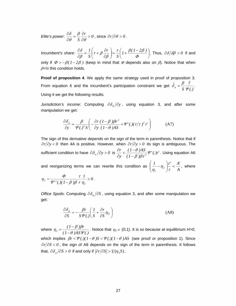
only if )21( ββΦ −−> (keep in mind that Φ depends also on β). Notice that when β<½ this condition holds. Proof of proposition 4. We apply the same strategy used in proof of proposition 3.

From equation 6 and the incumbent’s participation constraint we get (.)r

Sˆ

a Ψβδ = .

Using it we get the following results. Jurisdiction’s income: Computing ya ∂∂δ , using equation 3, and after some manipulation we get:

⎟⎟⎠

⎞⎜⎜⎝

⎛+

−−

∂∂

−=∂∂

')r(.)('AS)1(r)1(

yr

S(.)y2

2

2a ττΨ

θββ

Ψβδ

(A7)

The sign of this derivative depends on the sign of the term in parenthesis. Notice that if

0yr <∂∂ then 4A is positive. However, when 0yr >∂∂ its sign is ambiguous. The

sufficient condition to have 0ya >∂∂δ is '(.)')1(

AS)1(yr

2 τΨβτβ

θ−−

<∂∂

. Using equation A6

and reorganizing terms we can rewrite this condition as A'A'1

21

<⎟⎟⎠

⎞⎜⎜⎝

⎛−

ττη

η, where

01r)1(.)('' 1

2 >−

=η

τββΨ

Φη .

Office Spoils: Computing Sa ∂∂δ , using equation 3, and after some manipulation we get:

⎟⎠⎞

⎜⎝⎛

∂∂

+−=∂∂

3a

Sr

S1

(.)Sr

Sη

Ψβδ

(A8)

where (.)AS)1(

r)1(3 Ψθ

ββη−−

= . Notice that η3 ∈ (0,1). It is so because at equilibrium H>0,

which implies AS)1(.)(S)1(.)(r θΨθΨβ −<−< (see proof or proposition 1). Since 0Sr <∂∂ , the sign of A8 depends on the sign of the term in parenthesis. It follows

that, 0Sa >∂∂δ if and only if )(1 3SSr η>∂∂ .

28

Elite’s power: Computing θδ ∂∂ a , using equation 3, and after some manipulation we

get 0rS(.)3

a <∂∂

−=∂∂

θΨβη

θδ

.

Incumbent’s share: Computing βδ ∂∂ a , using equation 3, and after some manipulation we get:

⎟⎟⎠

⎞⎜⎜⎝

⎛∂∂

−=∂∂

3a r1

S(.)r βη

βΨβδ

(A9)

It is direct that if β>½, then 0r <∂∂ β and so 0a >∂∂ βδ . However, if β<½ the sign of

A9 is ambiguous. The sufficient condition to have 0a >∂∂ βδ is 21r βηβ <∂∂ , otherwise expression in A9 is negative. Centralized Model. Assume there are J>1 elites demanding corruption to the central incumbent (one in each of the J jurisdictions) indexed by j and endowed with economic power θj. At equilibrium, the citizens’ strategies are exactly the same we described in the decentralized game (see proof of proposition 1). Thus, let us study the behaviour of the rest of the players.

Elite j maximizes its payoff cj

cj

cj Hr)1( −−= βπ , subject to

cccc Srβδ ≤ (with

∑ == J

1jcj

c rr ), 0H cj ≥ , τ≤≤ c

jr0 , τ≤cr , and taking as given cir ji ≠∀ . The first

constraint implies ∑ ≠−⎟⎟

⎠

⎞⎜⎜⎝

⎛−

−≥

jici

cc

c

c

ccj H1S

r)r()1(AH τΨ

βθ

. Since cjπ strictly

decreases in cjH , then the elite chooses

∑ ≠−⎟⎟

⎠

⎞⎜⎜⎝

⎛−

−=

jici

cc

c

c

ccj H1S

r)r()1(AH τΨ

βθ

. It implies that at equilibrium

⎟⎟⎠

⎞⎜⎜⎝

⎛−

−= 1S

r)r()1(AH c

c

c

c

cc τΨ

βθ

, where ∑ == J

1jcj

c HH . We assume the

parameters of the model are such that 0H cj > . This reduces the elite j problem to the

following programme:

( ) ∑ ≠+⎟⎟

⎠

⎞⎜⎜⎝

⎛−

−−−= ji

ci

cc

c

c

ccj

ccjr

H1Srr)1(Ar)1(Max

j

τΨβθβπ

s.t. τ≤≤ cjr0 and τ≤cr

At equilibrium, the level of corruption in region j must satisfy:

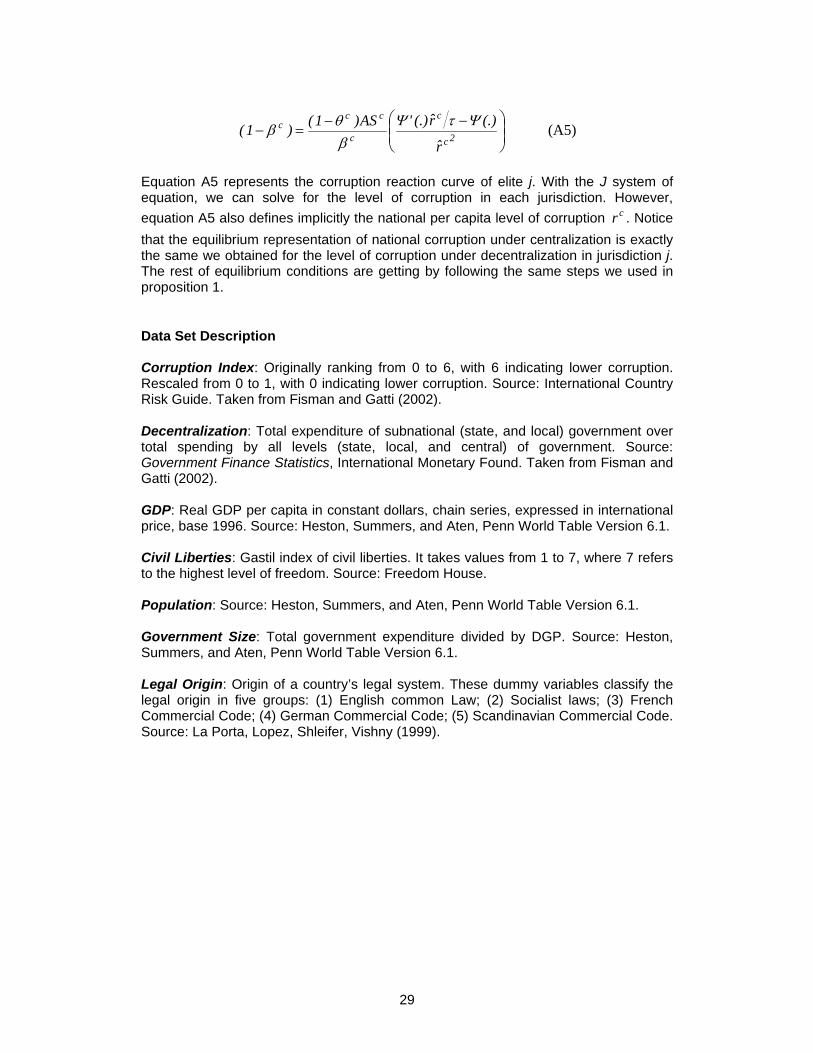
29

⎟⎟⎠

⎞⎜⎜⎝

⎛ −−=− 2c

c

c

ccc

r

(.)r(.)'AS)1()1( ΨτΨβθβ (A5)

Equation A5 represents the corruption reaction curve of elite j. With the J system of equation, we can solve for the level of corruption in each jurisdiction. However, equation A5 also defines implicitly the national per capita level of corruption cr . Notice that the equilibrium representation of national corruption under centralization is exactly the same we obtained for the level of corruption under decentralization in jurisdiction j. The rest of equilibrium conditions are getting by following the same steps we used in proposition 1. Data Set Description Corruption Index: Originally ranking from 0 to 6, with 6 indicating lower corruption. Rescaled from 0 to 1, with 0 indicating lower corruption. Source: International Country Risk Guide. Taken from Fisman and Gatti (2002). Decentralization: Total expenditure of subnational (state, and local) government over total spending by all levels (state, local, and central) of government. Source: Government Finance Statistics, International Monetary Found. Taken from Fisman and Gatti (2002). GDP: Real GDP per capita in constant dollars, chain series, expressed in international price, base 1996. Source: Heston, Summers, and Aten, Penn World Table Version 6.1. Civil Liberties: Gastil index of civil liberties. It takes values from 1 to 7, where 7 refers to the highest level of freedom. Source: Freedom House. Population: Source: Heston, Summers, and Aten, Penn World Table Version 6.1. Government Size: Total government expenditure divided by DGP. Source: Heston, Summers, and Aten, Penn World Table Version 6.1. Legal Origin: Origin of a country’s legal system. These dummy variables classify the legal origin in five groups: (1) English common Law; (2) Socialist laws; (3) French Commercial Code; (4) German Commercial Code; (5) Scandinavian Commercial Code. Source: La Porta, Lopez, Shleifer, Vishny (1999).