Čekerevac Z., DrSc, Associate Professor,

“Union“ University Belgrade, Faculty of Business Industrial Management

Živković D., MSc, Lecturer, Business School - Čačak

MANUFACTURING DISCRETE EVENTS SIMULATION

USING MS EXCEL AND VBA

Business decision making is certainly the most important task of every manager and it is often a very

difficult one. Decisions are made mostly in uncertain and dynamic environment where input variables are

subject of frequent change. Due to a large number of factors affecting a business, in the case of

manufacturing systems, it is almost impossible to develop only one, but adequate analytical model.

Therefore, researches use different simulation models to adequately represent different business systems.

Another big challenge for manufacturers is that commercial simulation software is very expensive. Creating

of such software requires enormous simulation expertise to construct a simulation program that is not

necessary in everyday simulation problems. Within this context, authors suggest to use spreadsheet as

simulation environment. For tactical simulation problems this article suggests a use of: Three-phase

simulation strategy, Activity Cycle Diagram (ACD), Visual Basic for Application and Microsoft Excel.

Using Excel has a lot of advantages, including Excel popularity and strong analytic and reporting tools.

Introduction. In today’s increasingly competitive world, simulation has become

an irreplaceable problem solving methodology for engineers, designers and

managers. Simulation is one of the most powerful tools available to decision-makers

responsible for business systems managing in general, and particularly manufacturing

systems. It makes possible to study, to analyze and to evaluate some specific business

situations that otherwise would not be possible. The use of spreadsheets, combined

with the Visual Basic for Application® (VBA) programming language, can become

powerful tool for simulation software implementation to conduct discrete event

simulation experiments.

Although the term simulation can have various meanings depending on its

application, it generally refers to use computer to perform experiments on a model of

real system. In other words, it is a process which mimics the relevant features of a

target process. Experiments by simulations may be undertaken before a real system is

operational, to support its design, to show how the system might react on changes in

its operational rules. Also, they allow evaluating the system’s responses on changes

in its structure. They are particularly suitable for situations when system is influenced

by great number of factors, and when great number of variables exists. In such

situations it is almost impossible to develop one and only adequate analytical model.

Real systems can be deterministic or stochastic, static or dynamic (with discrete

or continuous event). Depending of their characteristics, real systems can be

analyzed using various tools. For this study, of a special interest are stochastic

dynamic systems with discrete events. They are analyzed by using a discrete event

simulation (DEC) methodology.

Discrete event simulation is a kind of simulation where complex system and

processes are represented by the chronological sequence of events that comprise

them. To write simulation programs it is possible to use two kinds of computer

languages:

- General-purpose programming languages and

- Simulation oriented programming languages.

Both of them have their advantages and disadvantages. Model creation using

simulation software requires experience and/or training as well as good knowledge of

simulation theory. [1] [2] Alternative approach uses general-purpose programming

languages, and, for this analysis, the combination of Microsoft Office Excel® and

Visual Basic for Application (VBA) is chosen. Excel provides almost complete set of

tools for a simulation. [3] VBA, language for programming Microsoft Office

applications, is based on a core set of commands and extends on a per-application

basis. This means that VBA for Excel understand terms like workbook, worksheet,

cell and so on, while VBA for Access knows, among other things, about tables,

queries, reports, data entry forms.[4] Core part of VBA can be licensed to the third

party companies and used in their applications (for example Arena® Simulation

Software by Rockwell Automation). Excel-VBA combination has a lot of advantages.

Very important fact is that Excel has been very widely accepted by IT and ordinary

business people. Therefore, Excel can be used as good communication tool during

model development phase. Further Excel-VBA is very cheap compared with some

other simulation languages. There are also a number of other advantages, but it

should be mentioned that Excel-VBA combination is very suitable for solving a huge

number of everyday, tactical manufacturing problems. [5]

The essence or purpose of simulation modeling is to help decision-makers to

solve a problem. Therefore, they must merge problem solving techniques with

programming practice. One of the steps in this direction is conceptual model

formulation. This means preliminary model developing, either graphically (e.g. block

diagrams, Petri nets or process flow charts) or in pseudo-code (e.g. condition

specification), to define the components, descriptive variables and interactions (logic)

that constitute the system. For this phase it is suitable to use Activity Cycle Diagrams

(ACD) as a natural way to visually represent knowledge about a real system.

Conceptual model with ACD has network structure and represent logical and

temporal relationships among entity activities. For translation of ACD conceptual

models into computer models, in here applied discrete event simulator Michael

Pidd’s Three-phase approach [6] is used.

Activity Cycle Diagrams, Three-Phase Algorithm and Excel-VBA combination

are basic ingredients of here used discrete event simulator - DESim.

Activity cycle diagram and Three-Phase algorithm. The activity cycle

diagram (ACD) depicts the interaction of entities by composing their life’s cycles.

Here an entity means any component of a system which retains its identity through

time. ADC entities are divided into two types:

entities that are servers and

entities that are being served.

Activities to be constructed by the same resource(s) can be linked together

according to their logical sequence to form an activity chain, which is defined as the

activity cycle of the resource. The activity cycle of a resource may have only one

activity, and it should not be considered as a separate one if this activity can be

included in the activity cycle of another resource. An entity could be either in a

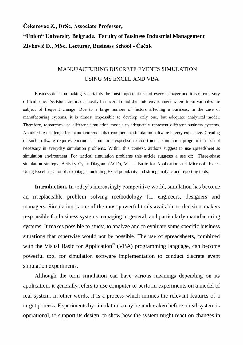
Passive State (in Queue) or in an Active State (in Activity). ACD graphical language

just requires the use three types of graphical objects: Rectangles (for activities),

Circles (for queues) and Arrows (for links). Sometimes, we use special symbol for

queue which represent environment. In this paper, environment queue is represented

with ellipse. For all symbols see Figure 1. It is important to note:

1 The duration of an activity is always known in advance (given by some

stochastic distribution), and an activity state usually involves the co-

operation of different types of entities. For an activity to start, it is necessary

that entities exist in the preceding queues in required numbers and with

adequate attributes. When these conditions hold, it is possible to start

activity. When the activity ends, the entities involved are moved to

consequent queues.

2 The duration of an entity in a queue cannot be known in advance.

3 In the ACD based three-phase approach each activity must begin, end, and

be executed.

4 Activities can be either bounded (begin and end time are known) or

conditional (resource must be available for the activity to begin).

Queue Environment Activity

Figure 1. Basic Elements of the ACD representation

There are some basic rules or conventions for constructing an ACD:

1 A Queue must contain only one type of entity.

2 Entity ACD consists of alternating sequence of the form: QUEUE –

ACTIVITY-QUEUE-ACTIVITY ... (when there are no reason for queuing

before an activity, dummy queues may be incorporated into the model).

3 All life cycles of each entity type should be closed.

In short, ACD uses three constructs to represent real systems: entity, queue

and activity. ACD model has activity world view, where a simulation analyst

thinks in terms of activities. [7]

The most common and classical example of an ACD representation is the

“English Pub Example”. Here, for brevity, we will show a simplified version. In

this case, the model contains three entities: “customer”, “bartender” and the

“entry”. After arrival, the customer waits for service. Bartender services

customers. When customer is serviced, he/she waits in ready queue for drinks.

The bartender either services customers or is idle. The entry could be blocked or

in arrival activity. The ACD for this simplified version of the „Pub” is showed in

figure 2.

Environment

DRINK

ARRIVAL

SERVICE

Idle

Wait

Preparation

Ready

Customer life cycle

Bartender life

cycle

Entry life cycle

Figure 2. Simplified ACD of the English Pub Model

Theoretical foundation for transformation of conceptual ACD simulation

model into computer program is Three-phase algorithm (TPA). Basic building

block of TPA is an activity and two events: the start of activity event and end of

activity event. Those events are considered to be activities of duration-zero time

units. With this definition, end of activity event is B activity (bound, planned to

occur) and start of activity event is C activity (conditional upon certain

conditions being true).

The 'three' in three-phase refers to the number of phases that are executed in

each cycle of the simulation. Job of each phase can be summarized as follows:

Phase 1: Determine when the next event in the simulation model is due.

This event will usually be completion of current/on-going activity.

Advance the simulation clock to the time of this event.

Phase 2: Execute the events identified in phase 1, this will usually

involve moving the entities from the activities that have just completed

into appropriate queues in the model.

Phase 3. Attempt any events in the model that are conditional in turn,

and execute those for which the conditions are satisfied. Repeat this

process until no more conditional events can take place (i.e. no more

activities can start).

These three phases are repeated until the simulation is complete – when the

terminating condition is reached, for example. Flow chart diagram of three-

phased algorithm is showed in Figure 3.

Start

Initialisation

Find next event and advance the clock to the time in

which this event is due

Execute all the B activities (the direct consequences

of the scheduled events) which are due at that time

The executive tries to execute all of the C activities

(any action whose start depends on resources and

entities whose state may have changed in B phase)

Simulation

finish ?

Simulation reports

Stop

A phase

B phase

C phase

No

Yes

Figure 3. Flow chart diagram of three-phase algorithm

Design and implementation. Idea behind this research is to design software

with VBA and Excel which enable user to take data from ACD and write them in

Excel worksheet, initiate simulation and get results of simulation also in Excel

worksheet. This approach simplifies the simulation task by automatic translation of

ACD into a computer model with very little or without additional programming. First

step in that direction is to extend convention ACD symbols for queue and activity.

After that, it is necessary to define rules on how to accept data into Excel worksheet

from ACD. Finally, according to those rules and three-phase algorithm, it is

necessary to write VBA programs to implement our discrete event simulator tool -

DESim.

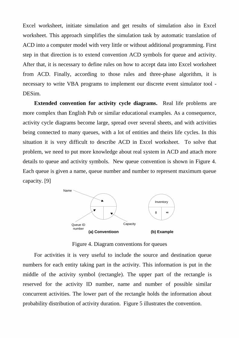
Extended convention for activity cycle diagrams. Real life problems are

more complex than English Pub or similar educational examples. As a consequence,

activity cycle diagrams become large, spread over several sheets, and with activities

being connected to many queues, with a lot of entities and theirs life cycles. In this

situation it is very difficult to describe ACD in Excel worksheet. To solve that

problem, we need to put more knowledge about real system in ACD and attach more

details to queue and activity symbols. New queue convention is shown in Figure 4.

Each queue is given a name, queue number and number to represent maximum queue

capacity. [9]

Name

Queue ID

number

Capacity

(a) Conventioon (b) Example

Inventory

8 ∞

Figure 4. Diagram conventions for queues

For activities it is very useful to include the source and destination queue

numbers for each entity taking part in the activity. This information is put in the

middle of the activity symbol (rectangle). The upper part of the rectangle is

reserved for the activity ID number, name and number of possible similar

concurrent activities. The lower part of the rectangle holds the information about

probability distribution of activity duration. Figure 5 illustrates the convention.

Activity

name

Activity ID

number

Concurrency

number

‘To’ queue

Statistical distribution

‘From’ queue

Entity name

5 Work center 1 1

8, Customer order, 12

20, Worker, 20

Normal(10,2)

(a) Convention (b) Example

Xx, nnnnn, yy

Figure 5. Diagram conventions for activities

Ready

10 1

Wait

30

∞

Envionment

50

Idle

20

1

Preparation

40

∞

∞

ARRIVAL1 1

10, Entry, 10

50, Customer, 20

3 DRINK m

40, Customer, 50

Normal(p3,q3)

2 SERVICE 1

20, Customer, 40

30, Bartender, 30

Normal (p2,q2)

Normal(q1,p1)

Figure 6. Application of new conventions for ACD from Figure 2

In the example the activity takes place when a 'Customer order' is available in

queue 8 and a 'Worker' in queue 20. Activity duration is normally distributed with a

mean of 10 minutes and standard deviation of 2 minutes. On completion of activity

'Customer order' moves to queue 12 and the 'Worker' returns to queue 20. Note that

it is necessary that names of queues and activities, and also queues ID numbers and

activities ID numbers, are unique. Figure 6 shows application of new conventions

based on ACD from Figure 2. Now, more information, about how the model

represents the real world, is available. In the model there is only one bartender.

Customer drinks only one beverage and leaves the pub. There are not any other

constraints, such as the pub capacity, number of glasses and so on. But model

simplicity does not hide the general idea of the design of a simulation tool.

So, all prerequisites to describe the conceptual model of the English Pub into

Excel worksheet are present.

Acceptation of the data into an Excel worksheet from ACD. There is a number of

ways to accept data into Excel worksheet from ACD, and one of them is design Excel

form, as shown on Figure 7. The form has five tabs:

1. General, initial tab with some help information.

2. Entities, for input of data about all entities in model.

3. Queues, for input of data about all queues in model.

4. Activities, for input of data about all activities in model.

5. Execution, for input of execution parameters, generates VBA code and

start simulation experiment.

When all ACD data are entered, it's time to start simulation. First task of

simulation program is to conduct verification of accepted data of conceptual model.

If all entered data are OK, simulation continues, otherwise, program generates error

message to inform user about nature of error(s).

Simulation model components for the DESim simulator where built using

Object-Oriented Programming and Discrete-Event Simulation concepts. These

reusable components were implemented in the class structure of the VBA. Because

we has limited space in this paper to describe structure of all VBA procedures, we

presents simulation object model on Figure 8 which shows how each of the

simulation component relate to each other in class hierarchy. Ours custom class

library is implemented in VBA. We hope that our approach how to design

simulation tool is sufficient clear. Focus of the rest of discussion on Initialization

procedure is on two classes: FutureEventList and RandomNumberGenerator.

Figure 7. Form for enter ACD model data into Excel worksheet

The mechanism for advancing simulation time and guaranteeing that all events

occur in correct chronological order is based on future event list (FEL). This list

contain all event notices for events that have been scheduled to occur at future time.

Scheduling a future event means that at the instant an activity begins, its duration is

computed from statistical distribution and the end-activity event, together with its

event time, is placed on the future event list. FEL is ordered by event time,

meaning that the events are arranged chronologically. Our FutureEventList class

has methods for put event on the list and get next event from the list.

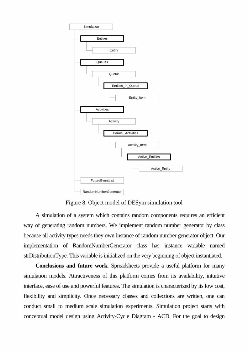
Simulation

Entities

Entity

Queues

Queue

Entities_In_Queue

Entity_Item

Activities

Activity

Paralel_Activities

Activity_Item

Active_Entities

Active_Entity

FutureEventList

RandomNumberGenerator

Figure 8. Object model of DESym simulation tool

A simulation of a system which contains random components requires an efficient

way of generating random numbers. We implement random number generator by class

because all activity types needs they own instance of random number generator object. Our

implementation of RandomNumberGenerator class has instance variable named

strDistributionType. This variable is initialized on the very beginning of object instantiated.

Conclusions and future work. Spreadsheets provide a useful platform for many

simulation models. Attractiveness of this platform comes from its availability, intuitive

interface, ease of use and powerful features. The simulation is characterized by its low cost,

flexibility and simplicity. Once necessary classes and collections are written, one can

conduct small to medium scale simulation experiments. Simulation project starts with

conceptual model design using Activity-Cycle Diagram - ACD. For the goal to design

Discrete Event simulation software - DESim, some modifications were made to standard

ACD. With those modifications it was put more knowledge about real system into ACD. It,

also, makes easier task of accepting ACD data into Excel spreadsheet.

Future work on DESim software should be concentrated on the following

improvements:

Use of the MS Office Visio as a graphical editor;

Extend semantics of ACD;

Improvement of reports on the simulation result, especially in the domain of

Excel graphical possibilities;

Design of the DESim software as Excel Add-on, and

Export and import of simulation data using XML or connecting with Access

database

With these improvements it is possible to get an easy-to-use, automated, robust and

flexible simulation modeling tool.

Works cited

1. Čerić V. Simulacijsko modeliranje/ V.Čerić// Školska knjiga, Zagreb.-1993.

2. Barlow J.F. Excel Models for Business and Operations Management/ J.F. Barlow//

John Wiley & Son.-2007.

3. Walkenbach J. Microsoft Office Excel 2007 Power Programming with VBA/J.

Walkenbach// Wiley Publishing Inc.-2007.

4. Getz K. and Gilbert M. VBA vodič za programere/ K. Getz and M. Gilbert// Mikro

knjiga, Beograd.-1997.

5. Green J. and all Excel®

2007 VBA Programmer’s Reference/ J. Green and all//

Wiley Publishing.-2007.

6. Pidd M. Computer Simulation in Management Science/ M. Pidd// John Wiley &

Sons.-1998.

7. Law A. M. Simulation Modeling & Analysis/ A.M. Law// McGraw – Hill. -2007.

8. Čekerevac Z. Upravljanje kvalitetom/ Z. Čekerevac// VPŠ Čačak.-2011.-ISBN 978-

86-7860-105-7