Contents lists available at ScienceDirect

Cement and Concrete Research

journal homepage: www.elsevier.com/locate/cemconres

Can the compressive strength of concrete be estimated from knowledge ofthe mixture proportions?: New insights from statistical analysis and machinelearning methodsBenjamin A. Younga, Alex Hallb, Laurent Pilona, Puneet Guptac, Gaurav Santd,e,f,⁎

a Department of Mechanical and Aerospace Engineering, Henry Samueli School of Engineering and Applied Science, University of California, Los Angeles, CA 90095, UnitedStatesb Suffolk Construction, Boston, MA 02119, United StatescDepartment of Electrical and Computer Engineering, Henry Samueli School of Engineering and Applied Science, University of California, Los Angeles, CA 90095, UnitedStatesd Laboratory for the Chemistry of Construction Materials (LC2), Department of Civil and Environmental Engineering, Henry Samueli School of Engineering and AppliedScience, University of California, Los Angeles, CA 90095, United Statese California Nanosystems Institute, University of California, Los Angeles, CA 90095, United StatesfDepartment of Materials Science and Engineering, Henry Samueli School of Engineering and Applied Science, University of California, Los Angeles, CA 90095, UnitedStates

A R T I C L E I N F O

Keywords:StrengthMixture designPredictive modelingMachine learningRegression analysis

A B S T R A C T

The use of statistical and machine learning approaches to predict the compressive strength of concrete based onmixture proportions, on account of its industrial importance, has received significant attention. However, pre-vious studies have been limited to small, laboratory-produced data sets. This study presents the first analysis of alarge data set (> 10,000 observations) of measured compressive strengths from actual (job-site) mixtures andtheir corresponding actual mixture proportions. Predictive models are applied to examine relationships betweenthe mixture design variables and strength, and to thereby develop an estimate of the (28-day) strength. Thesemodels are also applied to a laboratory-based data set of strength measurements published by Yeh et al. (1998)and the performance of the models across both data sets is compared. Furthermore, to illustrate the value of suchmodels beyond simply strength prediction, they are used to design optimal concrete mixtures that minimize costand embodied CO2 impact while satisfying imposed target strengths.

1. Introduction

A concrete's compressive strength after 28 days of aging is the mostcommonly used metric of its engineering properties and performanceand forms a critical input in structural design [1,2]. Indeed, structuralconcrete is most often specified on the basis of its compressive strengthafter 28 days of aging, and the compressive strength is known to beproportional to other mechanical properties such as the flexural andtensile strength [1]. Furthermore, it is well-known that concretestrength is chiefly influenced by w/c (water-to-cement ratio, massbasis). But, even for a given w/c, substantial variations in concretestrength may be observed based on the characteristics of constituentmaterials; e.g., cement type, the type of aggregate used, the pastecontent, mineral and chemical admixtures, etc. [1,2]. Therefore, a

robust, predictive model that could estimate compressive strength as afunction of the mixture proportions would be useful in enabling high-throughput mixture design, and reducing the empirical, labor intensivenature of “trial batching” approaches that are the basis of industrialpractice today.

Physical models that are capable of strength prediction (i.e., withoutempirical calibration) are difficult to construct, due to: (i) our inabilityto rigorously model cement hydration, and microstructure develop-ment, (ii) the unavailability of constituent material properties – forexample, while the mechanical properties of the constituent materials,and cement hydrates are better known, chemical data especially asneeded to model reaction kinetics is much less available [3–5], (iii)nonlinear elastic behavior of the cement paste which evolves with time[6–9], and (iv) the unpredictable effects of mineral and chemical

https://doi.org/10.1016/j.cemconres.2018.09.006Received 16 December 2017; Received in revised form 30 July 2018; Accepted 21 September 2018

⁎ Corresponding author at: Laboratory for the Chemistry of Construction Materials (LC2), Department of Civil and Environmental Engineering, Henry SamueliSchool of Engineering and Applied Science, University of California, Los Angeles, CA 90095, United States.

E-mail address: gsant@ucla.edu (G. Sant).

Cement and Concrete Research 115 (2019) 379–388

Available online 27 September 20180008-8846/ © 2018 Elsevier Ltd. All rights reserved.

T

admixture interactions, such as water-reducing admixtures (WRAs) orair-entraining admixtures (AEAs), on cement hydration and strengthdevelopment. Therefore, there is great interest in applying statisticaland machine learning (ML) methods (e.g. multiple linear regression,artificial neural networks) to model compressive strength evolution as afunction of the concrete's mixture proportions.

However, the vast majority of prior studies based on statistical orML approaches have been limited to smaller data sets consisting ofaround 1000 compressive strength measurements or less [10–19].Furthermore, these data sets typically encompass laboratory specimensproduced under controlled conditions. As such, it is unclear as to howwell these predictive models may perform when applied to data col-lected from industrial concrete production (“ready mix”) operations.This is because production data is likely to contain more unexplainablevariance whose effects on the accuracy of strength prediction modelsremains unknown. Therefore, the present study aims to evaluate theperformance of predictive models for estimating a concrete's compres-sive strength using a large data set of job-site based concrete strengthmeasurements.

2. Background

2.1. Machine learning/data mining algorithms

Machine learning and data mining algorithms that have been de-veloped over the past few decades provide a means of developingpredictive models from empirical data, without a need for detailedknowledge of the underlying physical mechanisms [20,21]. Therefore,such models may be well-suited for predicting a concrete's compressivestrength – a material property that can be influenced by compositional,processing and testing variables. This section provides a brief overviewof the modeling techniques used in this study while further details re-garding their formulation, and implementation can be found elsewhere[21].

2.1.1. Artificial neural networks (ANNs)Artificial neural networks (ANNs) are statistical models that seek to

determine input-output relationships via a series of connected datastructures or “neurons” [21,22]. The neurons are organized into layers,with each neuron being functionally related to all neurons in the pre-vious layer. Fig. 1 shows a schematic of a typical neural network modelwith p= 4 input variables, a hidden layer with k= 3 hidden neurons,and a single output.

Mathematically, the relationship between each hidden neuron andthe input variables can be expressed as [21],

=h w x( )iT

i (1)

where, x= [x1,…,xp]T is the vector of p input variables, wi = [wi, 1,…,wi, p]T are the “weights” corresponding to each input variable, and σis a nonlinear “activation function.” For regression problems, a sig-moidal function is most commonly used as the activation function, i.e.,[21],

=+ e

w x( ) 11

Ti w xi

T (2)

Similarly, the predicted output Y is related to the hidden neurons haccording to [21],

=Y g h( )T (3)

where, h= [h1,…,hk]T is the vector of hidden neuron values andβ= [β1,…,βk]T is another set of weight factors. Here again, g can be anonlinear function, however, it is typically taken as the identity matrixsuch that =Y hT .

Neural networks are “trained” by identifying the appropriate valuesof the weight factors w and β which minimize a measure of predictionerror for a given training data set. Often, the root-mean-squared error

(RMSE) provides an adequate measure of error, and can be expressedas,

==

Y YN

RMSE ( )

i

Ni i

1

2

(4)

where, Yi is the observed or measured output corresponding to ob-servation i, Yi is the predicted output, and N is the number of ob-servations or data points in the training set. Common numericalmethods such as the Levenberg–Marquardt algorithm [22], can be usedto identify the appropriate weight factors. The large number of fittingparameters in neural network models (i.e., the weight factors w and β)allows them to easily identify nonlinear interactions between inputvariables, resulting in a powerful predictive tool. But, if used indis-criminately, neural networks that have a large number of hidden layersand/or hidden neurons in each layer are prone to over-fitting data,leading to generalization errors [20,21]. Therefore, the size of a neuralnetwork should be chosen carefully based on cross-validation, as de-scribed below.

2.1.2. Decision treesDecision trees are a family of machine learning methods that can be

used for both data classification and regression problems [20,21,23]. Incontrast to neural networks, decision trees are “rule-based” models, i.e.,they aim to identify logical splits in the data rather than fit a set ofparameters in a mathematical formula. In other words, the tree splitsthe input space into a series of partitions or “leaf nodes,” and then usesa simple model (i.e., often simply a constant value) to predict the outputin each partition [21]. The splits are selected to minimize some metricof error, typically the sum-of-squared errors between predicted andobserved outputs (Eq. (4)). A popular method of determining the splitsis the classification and regression tree (CART) algorithm [23]. Clearly,the size of a tree must be limited in some way to prevent the tree frombecoming too large and over-fitting the data; this is typically done bylimiting the number of splits, or by ensuring that each leaf node con-tains a minimum number of data points [21,23].

The performance of decision tree regression models can be im-proved by building ensembles, or large collections of individual deci-sion trees, and aggregating their predictions. Such ensemble methodscan both increase prediction accuracy and reduce over-fitting andgeneralization errors [21]. One popular ensemble model is the so-calledrandom forest model, which trains a large number of trees individuallyusing only a random subset of the input variables [20,21]. In addition,each tree does not use the entire set of training data, but rather abootstrap sample of the training data [21]. This procedure is known asbootstrap aggregation or “bagging.” The predictions of each individualtree are then averaged to obtain the prediction of the random forestensemble. Gradient boosting [21] is another established tree ensemblemethod. In this case, an initial tree is trained using the entire set ofinput data and all input variables. Then, a second tree is trained to fitthe residuals of the first tree (i.e., the differences between the predictedand observed values) to the input data. This procedure is repeated for aspecified number of iterations (typically several hundred). Then, thepredictions of each tree are added to obtain the predictions of thegradient-boosted ensemble [20,21]. In order to avoid over-fitting, thecontribution of each tree beyond the first to the sum is reduced by afactor known as the learning rate, which typically varies between 0.01and 0.1 [20] and can be tuned by cross-validation.

2.1.3. Support vector machines (SVMs)Support vector machines (SVMs) are a family of regression models

that are effective for nonlinear problems [20,21,24,25]. Rather thanusing the sum-of-squared errors (Eq. (4)) as an objective function whenfitting the model, SVMs use another measure of error known as hingeloss or ε-insensitive loss. In this case, errors smaller than a set thresholdε do not contribute to the overall error measure. The hinge loss function

B.A. Young et al. Cement and Concrete Research 115 (2019) 379–388

380

can then be expressed as,

= <>

L Y Y Y YY Y Y Y

( ) 0 if | || | if | |

.i ii i

i i i i (5)

SVMs seek to fit a model of the form,

==

Y c kx x x( ) ( , )i

Ni i

1 (6)

where, the parameters ci are referred to as choice coefficients, and theGaussian kernel function k(x,xi) is defined as,

=k ex x( , ) .ix xi 2 (7)

This kernel function measures the similarity, quantified as aGaussian distance, between the set of inputs x and those of the ith pointin the training set xi. Note that because such a quantity is used, theinput data should be centered and scaled (i.e. subtracted from its meanand divided by its standard deviation) such that each variable is ren-dered unitless. Furthermore, Eq. (6) indicates that there are as manyparameters (the N choice coefficients) in the model as points in thetraining set. To make the problem mathematically feasible, a regular-ization term (i.e., a penalty term for large choice coefficients) must beadded to the objective function. The objective function can then beexpressed as,

= += = = =

J L Y c k c c kx x x x( , ) ( , ).i

N

ij

N

j i ji

N

j

N

i j i j1 1 1 1 (8)

The regularization factor λ determines how much the large choicecoefficients are penalized and should be tuned appropriately via cross-validation [21].

2.2. Previous studies on concrete strength prediction using statisticalmethods

Numerous authors have applied statistical and machine learningtechniques to predict the compressive strength of concrete based on itsmixture proportions [10–19]. Notably, Yeh et al. [10] published a

dataset consisting of 1031 measured compressive strengths as a func-tion of w/c, cement, fly ash and blast furnace slag contents, coarse andfine aggregate contents, superplasticizer dosage, and age, and usedartificial neural networks (ANNs) to develop a strength predictionmodel. The authors found that their ANN model offered a coefficient ofdetermination (R2) as high as 0.92 when comparing measured versuspredicted strengths on their test data. Several other studies[11,12,18,26] have used the same dataset published by Yeh et al. [10]to evaluate the performance of other machine learning models in pre-dicting compressive strength. These studies too have reported similarresults, with various models including neural networks [11,12],boosted and bagged regression trees [11], and SVMs [12] resulting inR2 > 0.9. In addition, other studies [13–17,19] have used different,smaller data sets to develop predictive models for compressive strength,primarily using neural networks [13–17,19]. Because most studies oncompressive strength prediction have used the same data set, or verysmall data sets secured under carefully-controlled laboratory condi-tions, it is unclear how well these predictive models can estimate thestrengths of industrially produced ready-mix concrete (RMC). This issignificant as in industrial operations, variables such as the ambienttemperature, type of mixing (central mixing, or truck mixing) or themoisture content of aggregates may be controlled imprecisely or not atall [27–29]. Therefore, one would expect the performance of predictivemodels to suffer from the extra noise introduced into the data by theseunobserved and/or uncontrolled variables.

The present study aims to quantify the extent of such noise on modelperformance, and identify if such uncontrolled parameters may induceunexplainable variance in compressive strength predictions of in-dustrially-produced concretes.

3. Analysis

3.1. Data collection

Two data sets were considered in this study. The first was the datasetpublished by Yeh et al. [10] consisting of 1031 measured compressivestrengths, as previously discussed. Because this data set has been used by

Fig. 1. A schematic of a typical feed-forward artificial neural network (ANN) with a single hidden layer.

B.A. Young et al. Cement and Concrete Research 115 (2019) 379–388

381

several previous studies, it provided a useful benchmark by which togauge model performance. Furthermore, as the present study is not fo-cused on the effect of age on concrete strength (N.B.: the 28 days strengthis most often captured during industrial production), only data forsamples with ages greater than or equal to 28 days were considered. Intotal, 706 of the 1031 measurements were used from the data set of Yehet al. while a subset of the data was neglected on account of havingstrengths measured before this 28-days reference age [10].

The second data set was provided by an international vertically-integrated cement/concrete producer (VIP) from across a range of dif-ferent concrete production sites and consisted of 9994 measured com-pressive strengths from job-site mixtures that were sampled acrossvarious locations in the United States. Three samples corresponding to agiven mixture was collected at the job-site (i.e., in the form of 6″ × 12″cylinders) and cured following ASTM C39 for 28 days after which timetheir compressive strengths were measured. The data set containedmixture proportions in terms of: w/c, cement and fly ash contents (in kgper m3 of concrete), water-reducing admixture (WRA) and air-en-training admixture contents (in kg per 100 kg of cementitious material),coarse and fine aggregate contents (in kg per m3 of concrete), and freshair content (in volume %) for each mixture. The mixture proportionsreported reflect the actual mixture proportions, i.e., based on the batchweights. Furthermore, all mixtures in the industrial dataset used ASTMC150 compliant Type I/II OPC. In general, Class F fly ash compliantwith ASTM C618 was used in all relevant cases. Finally, the aggregatesused were compliant with ASTM C33.

Prior to model training and evaluation, the VIP data set was subjectto a preprocessing step in which measurements that appeared to becorrupted by obvious recording/procedural errors were eliminated.However, measurements were not removed solely on the grounds ofbeing classified as outliers, as doing so would provide an overly opti-mistic view of performance. Indeed, robustness to such outliers is animportant quality of a useful predictive model, and care must be takento ensure that training and validation data are not manipulated ex-cessively prior to analysis.

To illustrate the variables in the data set, Fig. 2 plots the concrete'scompressive strength (fc, MPa) as a function of the eight input variablesin the VIP data set. As expected, there is an inverse relationship

between w/c and compressive strength, however, the range of mea-sured compressive strengths for a given w/c is still very large. Fur-thermore, it is difficult to recognize the effect of each input variable onthe compressive strength with seemingly no trends being visually evi-dent in the case of several (supposedly influential) input variables in-cluding: the fly ash content, fine aggregate content, etc.

3.2. Data splitting

In order to obtain estimates of the generalization error for thepredictive models developed in this study, each data set was partitionedinto training and test sets. The data was partitioned at random, witharound 80% of all data points used for training data and the remaining20% used for validation. For the Yeh et al. data set, 564 data pointswere used as training points while the remaining 142 were used asvalidation points. For the VIP dataset, the training set consisted of 7995measurements and the validation data set consisted of 1999 measure-ments. In each case, the training data set was used to develop and tunethe strength prediction models, while the validation data was used onlyfor final assessments of model performance.

3.3. Model tuning and cross-validation

Compressive strength prediction models were implemented followingfour distinct modeling approaches: neural network, gradient-boosted tree,random forest, and SVM. As discussed previously, each of these modelsinvolves a number of extra parameters that must be appropriately tunedto optimize performance. To accomplish this, a 5-fold cross-validation

Fig. 2. The relationship between the eight input (i.e., mixture proportion) variables and the concrete's compressive strength in the VIP's data set.

Table 1The parameters obtained following cross-validation for each compressivestrength prediction model.

Model Parameters

Neural network 2 hidden layers with 10 and 5 neurons eachRandom forest 500 trees in ensemble, 3 input variables used for each

treeGradient-boosted tree 500 trees in ensemble, learning rate = 0.09SVM ε = 2 MPa, λ= 13.5

B.A. Young et al. Cement and Concrete Research 115 (2019) 379–388

382

procedure was used [20,21] which consisted of the following steps:

1) To randomly partition the training set into 5 “folds”,2) To train the model using data from 4 of the 5 folds and use the 5th to

estimate the error,3) To repeat this procedure such that each of the 5 folds is used once to

estimate the error,4) To average the estimated errors from each of the 5 folds to obtain

the cross-validation error.

This procedure provides an estimate of the generalization errorwithin the same training sample. It can then be used to optimize themodel parameters by finding the values of the parameters that mini-mize the cross-validation error. Table 1 summarizes the parametersused by each model as tuned by cross-validation.

3.4. Concrete mixture optimization

The ability to estimate compressive strengths based on the mixtureproportions would allow a concrete producer to design and proportion“optimal” mixtures that minimize monetary cost and/or embodied CO2

impact, while still meeting a designer's strength requirements. Here,this is demonstrated by first identifying mixtures of minimal cost for agiven range of strengths (i.e., a two-objective optimization problem)and then identifying mixtures that minimize cost and embodied CO2

impact while still adhering to specified target strengths (three-objectiveoptimization). Because there are multiple objectives in each optimiza-tion scenario, there is no single optimal solution but rather a series ofoptimal (“Pareto”) solutions that emerge. Both optimization procedureswere conducted using the artificial neural network (ANN) modeltrained on the VIP dataset. This model is better suited for use in agradient-based optimization procedure because it is “smooth” with re-spect to the input parameters, as opposed to the tree-based modelswhich may contain non-differentiable points. The optimization wascarried out using the Broyden-Fletcher-Goldfarb-Shanno (BFGS) algo-rithm [30] within MATLAB's optimization toolbox. In an effort toidentify global rather than local optima, a pattern search method wasused to generate a large number of initial points. The optimization wasperformed for each of these points, and the best resulting solution wasconsidered as the global optimum.

Because concrete mixtures with a higher cementitious content havehigher compressive strengths, and because cementitious materials aremore expensive than aggregates, there is a trade-off between the ex-pected compressive strength and monetary cost of a mixture. The es-timated monetary costs of each mixture component on a mass basis arelisted in Table 2. The cost of mixing water was assumed to be negligible.The cost of fly ash can vary depending on location [31]; but to set arange, fly ash is proposed to cost between one-half to on par with ce-ment (i.e., ordinary portland cement, OPC) as noted below.

The objective function is the total cost of the concrete mixture per m3

of material, which can be expressed as,

= + + + +C p C p C p C p C pTotal cost ($/m ) c c fla fla fa fa ca ca WRA WRA3 (9)

where, Ci and pi are the dosage (in kg/m3) and cost (in $/kg) of mixturecomponent i, respectively. The optimization problem is defined by a

series of constraints, the first of which is that the compressive strength ofthe mixture must not be less than some target strength fc,target, such that:

f fx( )c pred c target, , (10)

where, fc,pred(x) is the compressive strength predicted by the neuralnetwork model as a function of the mixture parameters x. Next, it isnecessary that the sum of the volume fractions of each mixture compo-nent add up to one,

+ + + + + =C C C C C C 1c

c

w

w

fla

fla

fa

fa

ca

ca

WRA

WRA (11)

where, ρi is the density of each component (in kg/m3). Furthermore,upper and lower bounds were placed on some of the mixture parameters,as shown in Table 4. These bounds were based on the range of valuesobserved in the training fraction of the VIP data set; extrapolation be-yond them would likely lead to poor model performance and less certainresults.

The dosage of WRA was not treated as a free parameter – instead, itwas assumed to be directly proportional to the cementitious materialcontent at a mass ratio of 0.0031 kg WRA per kg of cement [35]. Fi-nally, in order to fully define the problem, the air content and AEAdosage (if present) are required as inputs to the strength predictionmodel. These parameters were assumed to be constant and to corre-spond to either air-entrained mixtures with an air content of 6 vol% andan AEA dosage of 0.03 mass % (by mass of cement), or to non-air-entrained mixes with an air content of 2 vol%; wherein no AEA isadded. These values were based on the average values in the VIP da-taset for air-entrained and non-air entrained concrete mixtures.

4. Results and discussion

4.1. Compressive strength prediction

Table 4 summarizes the performance of each model when applied tothe test set data from each of the two data sets. Three error metrics arereported, namely (i) root-mean-square error (RMSE, in MPa), (ii) R2-value (i.e., the strength of the linear relationship between predicted andobserved values), and (iii) mean absolute percentage error (MAPE). Forcomparison, the performance of a simple linear regression model of theform,

= +Y xT0 (12)

is also reported. First, Table 4 establishes that the R2-value of the pre-dictive models was higher when applied to the data set published byYeh et al. [10]. In other words, the models were able to explain more ofthe variance in compressive strength for this data set, as compared tothe job-site data from the VIP. However, the RMSE was also larger,indicating that the absolute compressive strength was predicted lessaccurately on average than for the VIP data set. Taken together, theseresults show that, unsurprisingly, the VIP data set features more un-explainable variance, than the data set of Yeh et al. Furthermore, whilethe more advanced models clearly out-performed the linear regressionmodel for the Yeh et al. data set, this difference was far less substantialfor the VIP data set; perhaps due to the increased noise (variance).

Overall, the contrast in model performance between data sets showsthat while statistical/ML models are very effective in predicting com-pressive strength of laboratory-curated mixtures based on their mixtureproportions, they are less effective in predicting the strength of concreteproduced in an industrial setting. To improve predictive performance inthe latter case, it may be necessary to expand the range of mixture(input) variables considered including: mixing temperature, mixingtype (central, or truck mixing), relative humidity, aggregate source andtype, moisture content, curing temperature profiles, potential job-siteretempering of the concrete (if any), uncertainty in batch weights,changes in cement, or fly ash behavior upon silo restocking, etc. Despite

Table 2The estimated bulk density and cost of each concrete mixture component.

Mixture component Subscript Density (kg/m3) Cost ($/kg) Ref.

Cement C 3150 0.110 [32]Water W 1000 0.000Fly ash fla 2500 0.055 [33]Coarse aggregate ca 2500 0.010 [32]Fine aggregate fa 2650 0.006 [32]WRA WRA 1350 2.940 [34]

B.A. Young et al. Cement and Concrete Research 115 (2019) 379–388

383

(a) (b)

(c) (d)

RMSE: 4.5 MPa RMSE: 4.8 MPa

RMSE: 4.4 MPa RMSE: 4.5 MPa

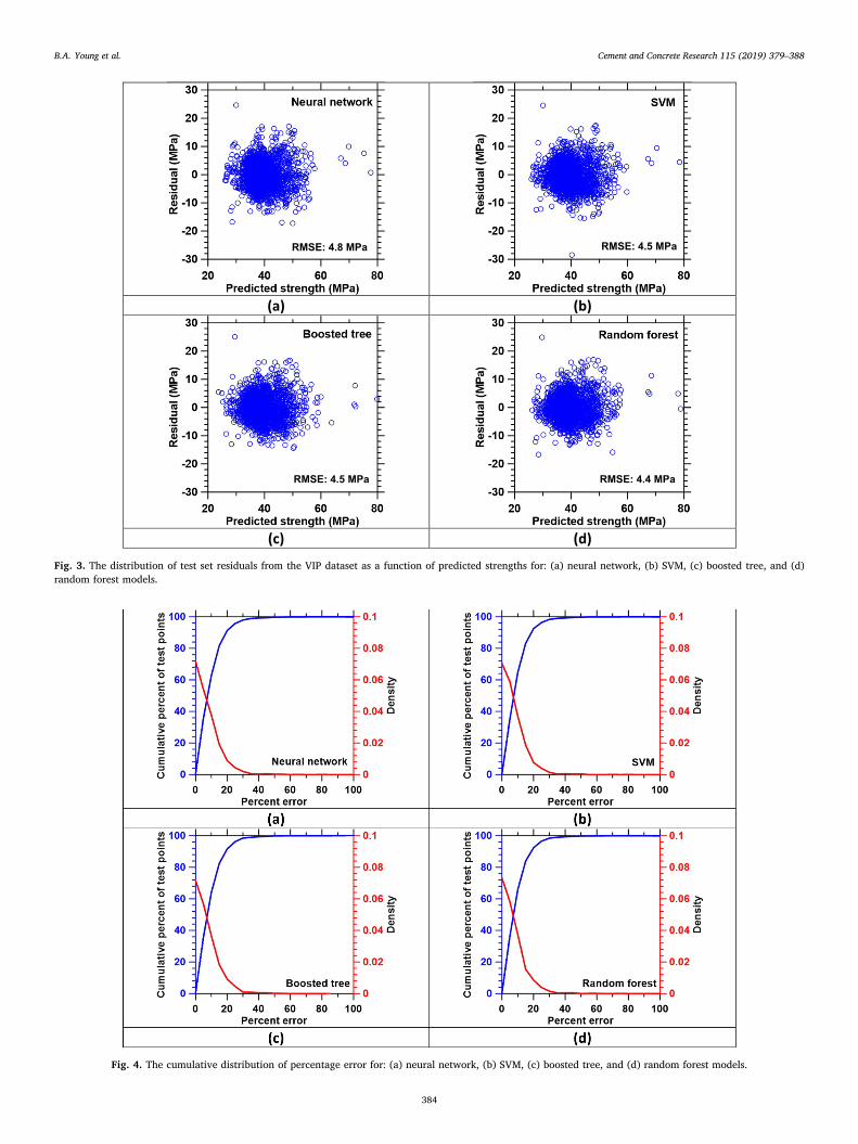
Fig. 3. The distribution of test set residuals from the VIP dataset as a function of predicted strengths for: (a) neural network, (b) SVM, (c) boosted tree, and (d)random forest models.

Fig. 4. The cumulative distribution of percentage error for: (a) neural network, (b) SVM, (c) boosted tree, and (d) random forest models.

B.A. Young et al. Cement and Concrete Research 115 (2019) 379–388

384

these shortcomings, each model was still able to predict compressivestrength with an average relative error of < 10% – a very favorableoutcome – even when applied to the industrial VIP data set. Further,while the performance of each machine learning method was similar,the random forest model exhibited the lowest RMSE and highest R2-value for both data sets. However, such small differences in perfor-mance between models suggest that each is equally well-suited forpredicting the compressive strength of industrial concrete, and there-fore, selection between them can be made based on their ease of im-plementation when used for a procedure such as the mixture optimi-zation examples that are demonstrated in the following section.

For clarity, Fig. 3 plots the test (validation data) set residuals fromthe VIP dataset (i.e., the difference between the measured and predictedstrengths) as a function of predicted strengths for each of the fourstatistical models considered, namely: (a) neural network, (b) SVM, (c)boosted tree, and (d) random forest. First, Fig. 3 shows that there is nosignificant correlation between the predicted strengths and the re-siduals. Additionally, the distribution of residuals is similar across eachof the four models. These observations are important because theysuggest that the errors in each model's predictions are due to un-explainable variance in the data, rather than due to the models failingto recognize important interactions between the input variables andcompressive strength. Finally, as an additional test of model perfor-mance, Fig. 4 plots the cumulative error distributions (i.e., showing thepercentage of test set points that are predicted within a given errorthreshold) for each of the four models, along with the empirical prob-ability density of the percentage errors. Indeed, each model was able topredict the strength within 10% relative error for over 60% of the testpoints, and within 20% error for over 80% of the test points. Onceagain, the performance of each model was similar, further reinforcing

the conclusion that each was able to identify the underlying patternsrepresented in the training dataset.

4.2. Mixture optimization

4.2.1. Cost-strength optimizationFig. 5 plots the minimum achievable mixture cost as a function of its

target strength (i.e., the “Pareto front”) for both: (a) air-entrained and(b) non-air entrained mixtures, computed via the previously describedoptimization procedure. Also shown are the predicted strengths andcosts of the mixtures from the VIP data set. In general, concrete mix-tures were considered to be air-entrained if they had an air content >4 vol% and non-air entrained otherwise [36]. It should be noted thatonly mixtures that conformed to the imposed optimization constraints(shown in Table 3) within ± 5% are shown. In general, Fig. 5 estab-lishes that all the job-site mixtures lie above the Pareto front, i.e., eachmixture has a higher estimated cost than necessary to achieve its targetstrength. It should be noted, however, that some of the mixtures offeredwithin the VIP dataset may have been subject to additional constraintsdepending on project specifications that were not considered in ouroptimization procedure.

Furthermore, Table 5 shows the resulting “optimal” mixture para-meters for various target strengths for both air-entrained and non-air-entrained mixes. As expected, the cementitious material content andthus the minimum achievable cost of each mixture increased with in-creasing target strength. Furthermore, the costs of air-entrained mixeswere higher, as higher air contents decrease the compressive strengthand thus must be compensated for by adding more cementitious ma-terial. Interestingly, most of the optimized mixtures contained themaximum allowable amount of fly ash, i.e., fly ash comprised 30% ofthe total cementitious material. This suggests that the reduction instrength arising from cement replacement by fly ash is more thancompensated for by 28 days by the reduced cost of the fly ash as

Fig. 5. The Pareto front showing the minimum possible (mixture) cost as a function of its target strength for: (a) air-entrained and (b) non-air entrained concretemixtures. Also shown are the estimated strengths and costs of mixtures from the VIP data set. These mixture optimizations were carried out using the ANN model.

Table 3The upper and lower bound constraints placed on the mixture parameters.

Mix parameter Expression Lowerbound

Upper bound

Cementitious material content Cc + Cfla 300 kg/m3 500 kg/m3

w/c Cw/(Cc + Cfla) 0.20 0.60Fly ash content Cfla 0 kg/m3 150 kg/m3

Coarse aggregate content Cca 500 kg/m3 1100 kg/m3

Fine aggregate content Cfa 600 kg/m3 1200 kg/m3

Fly ash/total cementitiousmaterial ratio

Cfla/(Cc + Cfla) 0.00 0.30

Total volume fraction ofaggregates

+Cfa

faCca

ca

0.60 0.75

Coarse/fine aggregate ratio CfaCca

0.50 1.00

Table 4A comparison of model performance in predicting the compressive strength foreach of the two data sets (Yeh et al. [10] and the VIP data set).

Model Yeh et al. dataset VIP data set

RMSE(MPa)

R2 MAPE (%) RMSE(MPa)

R2 MAPE (%)

Linear regression 8.8 0.66 22 5.0 0.49 10Neural network 6.3 0.82 14 4.8 0.54 9Random forest 5.7 0.86 14 4.4 0.60 9Boosted tree 5.8 0.85 13 4.5 0.59 9SVM 6.4 0.83 15 4.5 0.59 9

B.A. Young et al. Cement and Concrete Research 115 (2019) 379–388

385

compared to that of cement (N.B.: fly ash is assumed to cost 55% ofcement in this example). However, this nature of compensation is un-likely as the cost of fly ash increases, and the cost of fly ash and cementachieve parity. This is even more complicated by the fact that often,constraints on fly ash contents in industrial concretes are imposed dueto reduced rates of strength gain at early ages which results in reducedconstructability; a project specific constraint that cannot be genericallyfactored into approaches such as those demonstrated herein, i.e.,without introducing a penalty factor that assesses the financial impactof reduced strength gain rates.

Because the cost of fly ash might vary between regions, and fromseason to season, it is important to ascertain a “critical” fly ash costbeyond which the inclusion of fly ash (whether Class C or Class F) in aconcrete mixture is no longer an optimal choice – for cost minimization.To investigate these aspects, mixture optimization was performedacross a range of possible fly ash costs. As such, Fig. 6 plots the optimalratio of fly ash to total cementitious material as a function of the fly ashcost expressed as a percent of cement cost, for air-entrained concrete.Interestingly, for target strengths of 45 and 50 MPa, fly ash was stillpresent in the optimal mixture even when it was 90% as expensive as

cement. However, for a target strength of 55 MPa, fly ash was no longerincluded even when it was 75% as expensive as cement. This suggeststhat the inclusion of fly ash is a particularly effective cement dilutionapproach in conventional concrete mixtures, i.e., those which feature acompressive strength < 50 MPa.

4.2.2. Strength-cost-embodied CO2 optimizationAnother criterion that is expected to attain increasing prominence

for concrete mixtures is their embodied CO2 impact that is primarilyattributed to its cement (OPC) content. In general, industrial by-products (IBPs) such as fly ash are not attributed any embodied CO2

impact. The production of one metric ton of cement releases approxi-mately 900 kg of CO2 [37]. Therefore, the expected embodied CO2

impact of a concrete mixture (i.e., in kg of CO2 emitted per m3 ofconcrete produced) can be expressed as,

=CO 0.9Cembodied2, c (13)

where, Cc is the cement content of the concrete formulation. Thus, theprimary means of reducing embodied CO2 for conventional concretemixture is to substitute cement by fly ash (or another supplementarycementitious material, SCM, which in general have a lower embodiedCO2 impact than OPC). As shown in the previous section, substitutingcement by fly ash can reduce the cost of the formulation. However, it ispossible that in some cases, fly ash may be more expensive than cement.In this situation, there is a trade-off between minimizing cost andminimizing embodied CO2. In such cases, the mixture optimizationprocedure can be modified to account for such complexities by in-troducing an additional constraint given by,

0.9C COc 2,max (14)

where CO2,max is the maximum embodied CO2 (in kg/m3). In this case,optimal mixtures are those that not only fulfill the imposed targetstrength but also the imposed maximum embodied CO2 constraint.

Fig. 7 shows the Pareto front cost of optimal concrete mixtures as afunction of both the target strength and maximum embodied CO2 im-pact. As bounding cases, in Fig. 7(a), the price of fly ash was taken asone-half that of cement, whereas in Fig. 7(b) it was taken as 1.5 timesthat of cement. In Fig. 7(a), the curves overlap because both cost andembodied CO2 can be simultaneously minimized by replacing as muchcement as possible, by fly ash. This is because increasing the allowableembodied CO2, and allowing for increased cement content, doesnothing to reduce mixture cost. In contrast, Fig. 7(b) shows that in-creasing the embodied CO2 impact – and thus requiring less fly ash –leads to a lower cost. Furthermore, there were some cases when thetarget strength and embodied CO2 impact could not be achieved. Forexample, it was not possible to identify a mixture which featured astrength of 45 MPa but had an embodied CO2 impact of < 250 kg of

Table 5The optimized mixture parameters for concretes that achieve a series of target strengths, for both air-entrained and non-air entrained concrete formulations.

Target strength(MPa)

Min Cost($/m3)

Optimal mixture parameters Constraint values

w/c Fly ash(kg/m3)

Coarse aggregate(kg/m3)

Fine aggregate(kg/m3)

Total cementitiousmaterial (kg/m3)

Total agg.vol.%

Fly ash/cementitiousratio

Fine/coarseaggregate ratio

Air-entrained30 46.1 0.51 90 955 955 300 0.74 0.30 1.0035 46.3 0.6 90 1095 759 300 0.72 0.30 0.6940 53.6 0.6 58.3 1100 639 352 0.67 0.17 0.5845 60.1 0.24 129 1100 837 429 0.75 0.30 0.7650 62.7 0.25 138 1100 776 458 0.72 0.30 0.71

Non-air entrained30 45.6 0.60 90 946 899 300 0.72 0.30 0.9535 45.7 0.57 90 933 933 300 0.73 0.30 1.0040 46.2 0.49 90 963 963 300 0.75 0.30 1.0045 53.8 0.33 112 978 952 373 0.75 0.30 0.9750 55.7 0.29 117 965 965 392 0.75 0.30 1.00

Fig. 6. The optimal fly ash content expressed as a fraction of the total ce-mentitious content as a function of the price of fly ash scaled by the price ofcement. Cement is assumed to cost $ 0.110 per kg in this example. Thesemixture optimizations were carried out using the ANN model.

B.A. Young et al. Cement and Concrete Research 115 (2019) 379–388

386

CO2 per m3 of concrete produced. This nature of analyses offers themeans to rapidly screen, and eliminate unfeasible mixtures, and therebyconstrain and restrict (validatory) trial batching activities only to thosemixture formulations which are expected to feature the lowest cost, andembodied CO2 impact.

5. Summary and outlook

This study has examined the use of statistical and machine learningmethods to predict the compressive strength of concrete as a function ofits mixture proportions, so as to consequently improve the practice ofconcrete mixture design, quality control, and quality assurance. A largedataset with over 10,000 measured compressive strengths was obtainedfrom a vertically integrated cement/concrete producer (VIP) across arange of concrete production sites and used to train the predictivemodels. While the models have been shown to be very effective inpredicting compressive strength of laboratory-produced concrete sam-ples, they were less accurate when applied to the job-site data, possiblydue to additional noise introduced by uncontrolled or unreported pro-cess variables, and variance within the formulation, proportioning,mixture and casting, and testing process. However, despite this, themodels could still predict compressive strength with an average relativeerror of < 10%.

It should be noted however that the VIP data which spans a sub-stantial time-period of production includes diversity in: ambientweather conditions, the batches (and hence behavior) of cement and flyash used, mixing action (truck or central-plant mixing) and aggregatecomposition and grading as may be expected for large volume pro-duction operations. This is only further complicated by differences inhow water corrections are carried out and aggregate moisture content ismeasured which may be handled differently across different concreteproduction sites. These styles of differences may explain why themodeling approaches used herein are less effective at estimating job-site based concrete compressive strengths as compared to laboratorysourced data. This suggests a need to: (a) expand the size of the datasets used for training and testing the models, as doing so simultaneouslyimproves the ability of models to distinguish meaningful patterns in thedata from noise and allows for more refined hyperparameter tuningthrough cross-validation, and (b) incorporate a wider range of inputvariables for their influences on affecting concrete strength.

Finally, a mixture optimization procedure was demonstrated usingan ANN based strength prediction model to identify mixtures thatminimized the cost for a given target strength, while imposing limits onthe estimated embodied CO2 footprint of the mixture. These approachesoffer a means to rapidly screen promising formulations for more

intensive trial batching based evaluations – while reducing the laborand time intensity of concrete batching/trial operations. The outcomesof this paper are significant since they demonstrate a mathematicalbasis to estimate the strength of concrete – without a need for cementhydration, or microstructure models. Rather, the paper highlights thataccess to carefully curated large volumes of data, wherein the inputvariables are well-known (i.e., without needing to be carefully con-trolled) is a powerful means to apply big data analytics to rationalize,improve and accelerate concrete production operations: from the per-spective of performance, quality control, and robustness – while redu-cing material (over)use, and wastage, and limiting overdesign. Each ofthese aspects are valuable to enable the design of cost-efficient andenvironmentally-friendly concrete mixtures for the construction ofbuildings and infrastructure which are often substantially overdesignedon account of poor predictability of in-place engineering performance.

Acknowledgements

The authors acknowledge financial support for this research provi-sioned by: Infravation ERA-NET grant (ECLIPS: 31109806.0001), and,U.S. National Science Foundation (CAREER: 1253269). The authorsalso acknowledge financial support provided by the Office of the Vice-Chancellor for Research at UCLA via the ‘Sustainable L.A. GrandChallenge’. The contents of this paper reflect the views and opinions ofthe authors who are responsible for the accuracy of data presented. Thisresearch was carried out in the Laboratory for the Chemistry ofConstruction Materials (LC2) and Molecular Instrumentation Center atUCLA. As such, the authors gratefully acknowledge the support that hasmade these laboratories and their operations possible.

References

[1] M.L. Wilson, S.H. Kosmatka, Design and control of concrete mixtures, Skokie, Ill.:Portland Cement Assn, 15 edition, 2011.

[2] S. Mindess, J.F. Young, D. Darwin, Concrete, 2nd edition, Pearson, Upper SaddleRiver, NJ, 2002.

[3] J.J. Thomas, et al., Modeling and simulation of cement hydration kinetics andmicrostructure development, Cem. Concr. Res. 41 (12) (Dec. 2011) 1257–1278.

[4] K.O. Kjellsen, R.J. Detwiler, Reaction kinetics of portland cement mortars hydratedat different temperatures, Cem. Concr. Res. 22 (1) (Jan. 1992) 112–120.

[5] J.W. Bullard, et al., Mechanisms of cement hydration, Cem. Concr. Res. 41 (12)(Dec. 2011) 1208–1223.

[6] D.P. Bentz, Three-dimensional computer simulation of portland cement hydrationand microstructure development, J. Am. Ceram. Soc. 80 (1) (Jan. 1997) 3–21.

[7] Z.C. Grasley, D.A. Lange, Constitutive modeling of the aging viscoelastic propertiesof portland cement paste, Mech. Time-Depend. Mater. 11 (3–4) (Dec. 2007)175–198.

[8] R. Alizadeh, J.J. Beaudoin, L. Raki, Viscoelastic nature of calcium silicate hydrate,Cem. Concr. Compos. 32 (5) (May 2010) 369–376.

Fig. 7. The cost of optimized concrete mixes as a function of both their target strength and embodied CO2 impact for different minimum cement contents. To setbounds on the analysis, in (a) the price of fly ash was set as one-half that of cement, while in (b) it was set as 1.5 times higher than cement. The mixture optimizationswere carried out using the ANN model.

B.A. Young et al. Cement and Concrete Research 115 (2019) 379–388

387

[9] X. Li, Z.C. Grasley, J.W. Bullard, E.J. Garboczi, Computing the time evolution of theapparent viscoelastic/viscoplastic Poisson's ratio of hydrating cement paste, Cem.Concr. Compos. 56 (Feb. 2015) 121–133.

[10] I.-C. Yeh, Modeling of strength of high-performance concrete using artificial neuralnetworks, Cem. Concr. Res. 28 (12) (Dec. 1998) 1797–1808.

[11] J.-S. Chou, C.-K. Chiu, M. Farfoura, I. Al-Taharwa, Optimizing the prediction ac-curacy of concrete compressive strength based on a comparison of data-miningtechniques, J. Comput. Civ. Eng. 25 (May 2011) 242–253.

[12] K. O. Akande, T. O. Owolabi, S. Twaha, S.O. Olatunji, Performance comparison ofSVM and ANN in predicting compressive strength of concrete, IOSR J. Comput. Eng.16 (5) (2014) 88–94.

[13] M.H.F. Zarandi, I.B. Türksen, J. Sobhani, A.A. Ramezanianpour, Fuzzy polynomialneural networks for approximation of the compressive strength of concrete, Appl.Soft Comput. 8 (1) (2008) 488–498.

[14] U. Atici, Prediction of the strength of mineral admixture concrete using multi-variable regression analysis and an artificial neural network, Expert Syst. Appl. 38(8) (2011) 9609–9618.

[15] J. Kasperkiewicz, J. Racz, A. Dubrawski, HPC strength prediction using artificialneural network, J. Comput. Civ. Eng. 9 (4) (1995) 279–284.

[16] H. Ni, J. Wang, Prediction of compressive strength of concrete by neural networks,Cem. Concr. Res. 30 (8) (2000) 1245–1250.

[17] A. Öztaş, M. Pala, E. Özbay, E. Kanca, N. Caglar, M.A. Bhatti, Predicting the com-pressive strength and slump of high strength concrete using neural network, Constr.Build. Mater. 20 (9) (2006) 769–775.

[18] M.H. Rafiei, W.H. Khushefati, R. Demirboga, H. Adeli, Supervised deep restrictedBoltzmann machine for estimation of concrete, ACI Mater. J. 114 (2) (2017).

[19] I.B. Topcu, M. Sarıdemir, Prediction of compressive strength of concrete containingfly ash using artificial neural networks and fuzzy logic, Comput. Mater. Sci. 41 (3)(2008) 305–311.

[20] M. Kuhn, K. Johnson, Applied Predictive Modeling, Springer, New York, NY, 2013.[21] Z.Q. John Lu, The elements of statistical learning: data mining, inference, and

prediction, J. R. Stat. Soc. A. Stat. Soc. 173 (3) (Jul. 2010) 693–694.

[22] H.B. Demuth, M.H. Beale, O. De Jess, M.T. Hagan, Neural Network Design, 2nd ed.,Martin Hagan, USA, 2014.

[23] L. Breiman, J. Friedman, C.J. Stone, R.A. Olshen (Eds.), Classification andRegression Trees, UK ed., Chapman and Hall/CRC, Boca Raton, 1984.

[24] M.C. Mozer, M.I. Jordan, T. Petsche, Advances in Neural Information ProcessingSystems 9: Proceedings of the 1996 Conference, MIT Press, 1997.

[25] The Nature of Statistical Learning Theory Vladimir Vapnik Springer.[26] N.K. Nagwani, S.V. Deo, Estimating the concrete compressive strength using hard

clustering and fuzzy clustering based regression techniques, Sci. World J. 2014(Oct. 2014) e381549.

[27] K. Wang, J. Hu, Use of a moisture sensor for monitoring the effect of mixing pro-cedure on uniformity of concrete mixtures, J. Adv. Concr. Technol. 3 (3) (2005)371–383.

[28] Z. Bofang, Thermal Stresses and Temperature Control of Mass Concrete,Butterworth-Heinemann, 2013.

[29] G.H. Tattersall, Workability and Quality Control of Concrete, CRC Press, 2003.[30] “Wiley: Practical Methods of Optimization, 2nd edition - R. Fletcher.” ([Online].

Available: http://www.wiley.com/WileyCDA/WileyTitle/productCd-0471494631.html. Accessed: 15-Sep-2017).

[31] M. Ahmaruzzaman, A review on the utilization of fly ash, Prog. Energy Combust.Sci. 36 (3) (Jun. 2010) 327–363.

[32] U.S. Geological Survey, Mineral Commodity Summaries, (2017).[33] Ashgrove Cement Company, ASTM Class F Fly Ash Information Sheet, (1999).[34] M. Collepardi, Admixtures used to enhance placing characteristics of concrete, Cem.

Concr. Compos. 20 (2) (Jan. 1998) 103–112.[35] B.A.S.F. Corporation, MasterGlenium 7500 Product Data Sheet, (2015).[36] Portland Cement Association, Control of Air Content in Concrete, (Apr. 1998).[37] N. Mahasenan, S. Smith, K. Humphreys, The cement industry and global climate

change: current and potential future cement industry CO2 emissions, in: J. Gale,Y. Kaya (Eds.), Greenhouse Gas Control Technologies - 6th InternationalConference, Pergamon, Oxford, 2003, pp. 995–1000.

B.A. Young et al. Cement and Concrete Research 115 (2019) 379–388

388