central east pacific flight routing - nasa

American Institute of Aeronautics and Astronautics1

Central East Pacific Flight Routing

Shon Grabbe* and Banavar Sridhar†

NASA Ames Research Center, Moffett Field, CA, 94035-1000

Nadia Cheng‡

University of California—San Diego, La Jolla, CA, 92093-0411

This paper examines the potential benefits of transitioning from the fixed Central EastPacific routes to user-preferred routes. A minimum-travel-time, wind-optimal dynamicprogramming algorithm was developed and utilized as a surrogate for the actual user-provided routing requests. After first describing the characteristics of the flights utilizingthe Central East Pacific routes for a five-day period, the results of both nominal and wind-optimal routing simulations are presented. The average potential time and distance savingsfor the wind-optimal routes was 9.9 min and 36 nmi per flight, respectively. When the wind-optimal routing flight plan deviations were confined within the oceanic center boundary, theaverage potential time and distance savings were 4.8 min and 4.0 nmi per flight, respectively.These results are likely an upper bound on the potential savings due to the location of thepolar jet stream during this five-day period. Although the sector loading did notsignificantly change under the wind-optimal routing simulations, the number of simulatedfirst-loss-of-separation events did, which could contribute to increased controller workload.

I. Introductionhe Oakland Oceanic Flight Information Region (FIR) (or Center), which is shown in Fig. 1, controlsapproximately 21.3 million square miles of airspace and borders the Anchorage FIR to the north, the Tokyo FIR

to the west, the Aukland FIR to the south, and the coastline of the contiguous United States on the east.1 In contrast,the twenty Air Route Traffic Control Centers (ARTCCs) in the contiguous U.S. encompass roughly 3 million squaremiles. Despite the vast amount of airspace controlled by Oakland Center, flights, for the most part, are required tofly along fixed route structures and adhere to lateral separation standards that extend up to 100 nmi, longitudinalseparation standards extending up to 15 min, and vertical separation standards of 1000 ft.2 These stringentseparation standards are required because of the limited surveillance capabilities in the ocean and the FAA’s legacyOceanic Display and Planning System (ODAPS).

With the introduction of the FAA’s new Advanced Technologies & Oceanic Procedures (ATOP) at OaklandCenter in 2005, increased route flexibility and reduced separation standards can potentially be accommodated.Some of the major ATOP innovations leading to this increased flexibility are (1) fully integrated flight- and radar-data-processing capabilities, (2) conflict-detection capabilities, and (3) satellite data-link communication andsurveillance capabilities.3 This paper presents the results of a study examining the potential benefits andconsequences of allowing user-preferred routing in place of the fixed Central East Pacific (CEP) routes.

* Research Scientist, Automation Concepts Research Branch, Mail Stop 210-10, [email protected].† Chief, Automation Concepts Research Branch, Mail Stop 210-10, Fellow AIAA.‡ Student, Dept. of Mechanical and Aerospace Engineering.

T

AIAA Guidance, Navigation, and Control Conference and Exhibit21 - 24 August 2006, Keystone, Colorado

AIAA 2006-6773

This material is declared a work of the U.S. Government and is not subject to copyright protection in the United States.


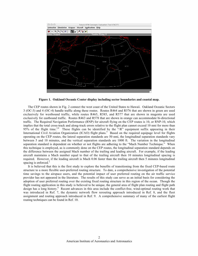
Figure 1. Oakland Oceanic Center display including sector boundaries and coastal map.

The CEP routes shown in Fig. 2 connect the west coast of the United States to Hawaii. Oakland Oceanic Sectors3 (OC-3) and 4 (OC-4) handle traffic along these routes. Routes R464 and R576 that are shown in green are usedexclusively for westbound traffic, while routes R465, R585, and R577 that are shown in magenta are usedexclusively for eastbound traffic. Routes R463 and R578 that are shown in orange can accommodate bi-directionaltraffic. The Required Navigation Performance (RNP) for aircraft flying on the CEP routes is 10, or RNP-10, whichimplies that the total cross-track and along-track errors relative to the flight plan cannot exceed 10 nmi for more than95% of the flight time.2,4 These flights can be identified by the “/R” equipment suffix appearing in theirInternational Civil Aviation Organization (ICAO) flight plans.5 Based on the required equipage level for flightsoperating on the CEP routes, the lateral separation standards are 50 nmi, the longitudinal separation standards varybetween 5 and 10 minutes, and the vertical separation standards are 1000 ft. The variation in the longitudinalseparation standard is dependent on whether or not flights are adhering to the “Mach Number Technique.” Whenthis technique is employed, as is commonly done on the CEP routes, the longitudinal separation standard depends onthe difference between the assigned Mach number of the trailing and leading aircraft. For example, if the leadingaircraft maintains a Mach number equal to that of the trailing aircraft then 10 minutes longitudinal spacing isrequired. However, if the leading aircraft is Mach 0.06 faster than the trailing aircraft then 5 minutes longitudinalspacing is enforced.2

It is believed that this is the first study to explore the benefits of transitioning from the fixed CEP-based routestructure to a more flexible user-preferred routing structure. To date, a comprehensive investigation of the potentialtime savings to the airspace users, and the potential impact of user preferred routing on the air traffic serviceprovider has not appeared in the literature. The results of this study can serve as an initial basis for considering theadoption of user preferred routing over the existing fixed routing structure in this region of the ocean. Though theflight routing application in this study is believed to be unique, the general area of flight plan routing and flight pathdesign has a long history.6 Recent advances in this area include the conflict-free, wind-optimal routing work thatwas introduced in Ref. 7, the dynamic network flow rerouting approach introduced in Ref. 8, and the fleetassignment and routing approach introduced in Ref. 9. A comprehensive summary of many of the earliest flightrouting techniques can be found in Ref. 10.


Figure 2. Central East Pacific (CEP) routes.

The rest of this paper is organized as follows. Section II describes the wind-optimal routing method that wasadopted for this paper. The unmodified characteristics of the CEP routes are described in Section III and themodeling results are presented in Section IV. Finally, Section V ends with some conclusions.

II. Modeling MethodWith ATOP, it is now conceivable to transition from the fixed CEP route structure in the Pacific to a set of

routes that accommodate the airline user’s preferences, which are assumed to be wind-optimal for this study. Tobegin understanding the potential implications of this transition, a minimum-travel-time, wind-optimal dynamicprogramming (DP) algorithm was developed to simulate possible user route preferences. Though the businessmodels, schedules, and aerodynamic performance characteristics of the aircraft in the airline’s fleet will ultimatelygovern the design of the optimal trajectories each airline wishes to fly, a simple minimum-time wind-optimal modelshould initially suffice to understand this change in routing philosophy. The remainder of this section is organizedas follows. In Section II.A, the standard dynamic programming recursion relation will be presented, and detailsconcerning the dynamic programming grid are presented in Section II.B.

A. Dynamic Programming Recursion RelationThe position of an aircraft along a minimum-time wind-optimal route at stage k+1 can be related to the position

at stage k via the following equation:

€

xk+1 = xk + uk (1)

Here

€

uk is the decision variable at stage k. Wind-optimal routes are then calculated on a grid composed of latitudeand longitude values that encompasses the region of airspace in which each aircraft travels. Though the grid isindividually tailored for each flight, it is roughly bounded between the 20o north latitude to the south, 40o northlatitude to the north, 156o west longitude to the west, and 120o west longitude to the east. This grid is sufficient formost flights that either depart or arrive at the west coast of the United States. For flights departing or arriving atinland airports, such as Chicago O’Hare International Airport, the grid is increased accordingly.

Within this problem formulation, the states

€

xk refer to the set of latitude/longitude points,

€

(λk ,τ k ) that areavailable at stage k; and the decision variable

€

uk represents the set of admissible changes in latitude and longitudethat are permitted at each stage. The admissible states and decision variables that are available at each stage will bediscussed in more detail in Section II.B.


Using the principle of optimality, the minimum cost function at stage k,

€

I (x,k) , can be calculated from theminimum cost function at stage k+1,

€

I (xk + uk ,k +1) using the following expression:11

€

I (x,k) = minuk ∈Uk

C xk ,uk ,k( ) + I (xk + uk ,k +1){ } for

€

k ∈ 0,1,...,N −1{ } (4)

Here

€

C (xk ,uk ,k) is the incremental cost associated with transitioning from state

€

xk to

€

xk+1 using the decisionvariable

€

uk at stage k. For our study, the cost is equal to the amount of time required for an aircraft to fly from thecurrent state,

€

xk , to the next state,

€

xk+1. The details of the cost function calculations are provided in the Appendix.The sequence of controls (i.e.,

€

u0,u1,K,uN−1) resulting from the solution of Eq. 4 for

€

0 ≤ k ≤ N −1 is used toconstruct the minimum-time, wind-optimal routes between the origin and destination airport for each flight. For allroutes generated using Eq. 4, the minimum cost function at k=N (i.e.,

€

I (x,N ) ) has been set to zero.To illustrate the use of this algorithm, wind-optimal trajectories for the east- and westbound aircraft that were

nominally flying on the CEP routes are presented in the fourth section of this paper.

B. Dynamic Programming GridFor a given starting- and end-point, the process of generating the set of admissible states and decision variables

for use in Eq. (4) involves three steps. In the first step, a series of

€

(N mid − 2) intermediate, equally spaced points isgenerated along the great circle route connecting the starting- and end-point. If the ending point (i.e., the originairport) is denoted by

€

(λ0mid ,τ 0

mid ) and the starting point (i.e., the destination airport) is denoted by

€

(λN midmid ,τ N mid

mid )

then the remaining

€

(N mid − 2) points are given by12

€

λ imid = tan−1(zi / (xi

2 + yi2)) (5)

€

τ imid = tan−1(yi / xi) (6)

where

€

xi = Ai cosλ0mid cosτ 0

mid + Bi cos λN midmid cosτ N mid

mid (7)

€

yi = Ai cosλ0mid sinτ 0

mid + Bi cosλN midmid sinτ N mid

mid (8)

€

zi = Ai sinλ0mid + Bi sinλN mid

mid (9)

€

Ai = sin((1− f i)d0→N midmid /sind0→N mid

mid ) (10)

€

Bi = sin( f id0→N midmid ) /sind0→N mid

mid (11)

Here

€

f i ∈ {x ∈ ℜ | 0 ≤ x ≤ 1} is the fraction of the distance between the starting and end points at which to create a

new intermediate point and

€

d0→N midmid is the great circle distance between the starting and end points that can be

calculated from Eq. (16) in the Appendix. A simple example in which

€

N mid = 4 and

€

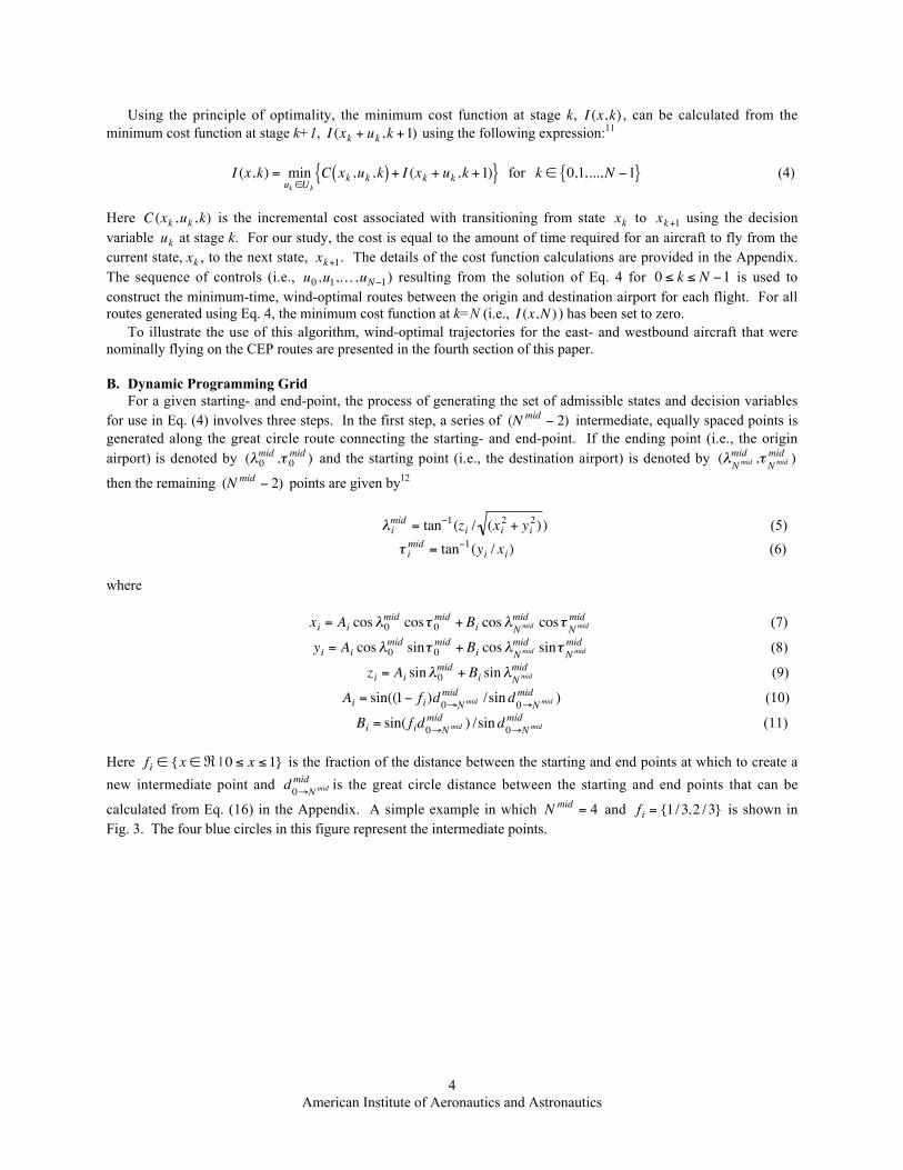
f i = {1/3,2 /3} is shown inFig. 3. The four blue circles in this figure represent the intermediate points.


Figure 3. Sample dynamic programming grid.

The second step in creating the latitude and longitude grid entails the calculation of the upper and lower pointsthat are depicted by the red and green circles, respectively, in Fig. 3. These offset points (i.e., the lower and upperpoints) are calculated using the following methodology:

€

λ ioffset = sin−1 sinλ i

mid cos doffset + cosλ imid sindoffset cosφi[ ] (12)

€

Δτ ioffset = tan−1 sinφi sindi→ j

mid cos λ imid /(cos di→ j

mid − sinλ imid sinλ i

offset )[ ] (13)

€

τ ioffset = mod(τ i

mid − Δτ i + π ,2π ) − π (14)

Here

€

φi =θ i→ jmid ± niΔθ where

€

θi→ jmid is the great circle course angle between the

€

i thand

€

j thmid-point,

€

ni ∈ [1,K,N offset ] is the index of the

€

i th upper/lower offset point,

€

N offset is the number of upper or lower offsetpoints, and

€

Δθ is the upper/lower angular offset. Using the positive sign in the expression for

€

φi gives rise to thepoints that will be referred to as the “upper-offset” points, while the negative sign in this expression will be usedwhen generating the “lower-offset” points. Additionally,

€

doffset is the distance from the

€

i th mid-point at which to

construct the upper/lower offset point, and

€

di→ jmid is the great circle distance between the

€

i th and

€

j th midpoint. It is

important to note that collectively, the set of midpoints, upper-offset points, and lower-offset points comprise thecomplete set of states,

€

xk , that are discussed in Section II.A.The last and final step of the DP grid generation process entails connecting the relevant midpoints and the

upper/lower-offset points (i.e., the states,

€

xk ). This process effectively defines the set of admissible controls,

€

Uk ,

that are available at each stage. Starting with the midpoints, a segment is drawn that connects

€

(λ imid ,τ i

mid )with

€

(λ i−1mid ,τ i−1

mid ) and

€

2N offset segments are drawn between

€

(λ imid ,τ i

mid ) and

€

(λ i−2offset ,τ i−2

offset ) . Notice that the

existence of

€

N offset upper points and

€

N offset lower points are assumed. Using this process, the seven dashed, blueedges depicted in Fig. 3 are constructed. Next, segments are drawn that connect each upper/lower offset point,

€

(λ ioffset ,τ i

offset ) , with their respective upper/lower points denoted by

€

(λ i+1offset ,τ i+1

offset ) . Note that the upper and lower

offset points are not connected as part of this process (e.g., in Fig. 3,

€

(λ0upper ,τ 0

upper ) is not connected to

€

(λ1lower ,τ1

lower)). Finally, the upper/lower-offset points are connected to the midpoints by constructing a segment

between

€

(λ ioffset ,τ i

offset ) and

€

(λ imid ,τ i

mid ) . This process of constructing connecting segments that originate at theupper/lower-offset points, gives rise to the three solid-red segments and three dash-dot-green segments in Fig. 3.


Once a grid has been created, the recursion relation presented in Eq. (4) is used to incrementally construct thewind-optimal route from the destination airport that is labeled “START” in Fig. 3 to the origin airport that is labeled“END.” The optimal sub-route to any node in this grid is determined by calculating the minimum total incrementalcost associated with traveling from the “START” node to the node of interest. For example, to calculate the optimalsub-route from the “START” node to the node labeled

€

(λ0lower ,τ 0

lower) the minimum of

€

C (λ0lower ,τ 0

lower )→ (λ2mid ,τ 2

mid )( ) +C (λ2mid ,τ 2

mid ) and

€

C (λ0lower ,τ 0

lower )→ (λ1lower ,τ1

lower )( ) +C (λ1lower ,τ1

lower ) is

selected. Here

€

C (λ0lower ,τ 0

lower )→ (λ2mid ,τ 2

mid )( ) is the cost associated with routing from

€

(λ0lower ,τ 0

lower) to

€

(λ2mid ,τ 2

mid ) using Eq. (15),

€

C (λ0lower ,τ 0

lower )→ (λ1lower ,τ1

lower )( ) is the cost associated with routing from

€

(λ0lower ,τ 0

lower) to

€

(λ1lower ,τ1

lower) ,

€

C (λ2mid ,τ 2

mid ) is the minimum incremental cost to arrive at

€

(λ2mid ,τ 2

mid ) from

“START,” and

€

C (λ1lower ,τ1

lower ) is the minimum incremental cost to arrive at

€

(λ1lower ,τ1

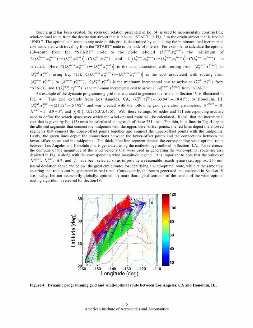
lower) from “START.”An example of the dynamic programming grid that was used to generate the results in Section IV is illustrated in

Fig. 4. This grid extends from Los Angeles, CA,

€

(λ5mid ,τ 5

mid ) = (33.94o,−118.41o) , to Honolulu, HI,

€

(λ0mid ,τ 0

mid ) = (21.32o,−157.92o) and was created with the following grid generation parameters:

€

N offset = 10 ,

€

N mid = 5,

€

Δθ = 3o , and

€

f i ∈ {1/5,2 /5,3/5,4 /5} . With these settings, 86 nodes and 751 corresponding arcs areused to define the search space over which the wind-optimal route will be calculated. Recall that the incrementalcost that is given by Eq. (15) must be calculated along each of these 751 arcs. The thin, blue lines in Fig. 4 depictthe allowed segments that connect the midpoints with the upper/lower-offset points; the red lines depict the allowedsegments that connect the upper-offset points together and connect the upper-offset points with the midpoints.Lastly, the green lines depict the connections between the lower-offset points and the connections between thelower-offset points and the midpoints. The thick, blue line segment depicts the corresponding wind-optimal routebetween Los Angeles and Honolulu that is generated using the methodology outlined in Section II.A. For reference,the contours of the magnitude of the wind velocity that were used in generating the wind-optimal route are alsodepicted in Fig. 4 along with the corresponding wind magnitude legend. It is important to note that the values of

€

N offset ,

€

N mid ,

€

Δθ , and

€

f i have been selected so as to provide a reasonable search space (i.e., approx. 250 nmilateral deviation above and below the great circle route) for identifying a wind-optimal route, while at the same timeensuring that routes can be generated in real time. Consequently, the routes generated and analyzed in Section IVare locally, but not necessarily globally, optimal. A more thorough discussion of the results of the wind-optimalrouting algorithm is reserved for Section IV.

Figure 4. Dynamic programming grid and wind-optimal route between Los Angeles, CA and Honolulu, HI.


III. Unmodified Flow CharacteristicsThis section describes the data sources used and familiarizes the reader with the nominal characteristics of the

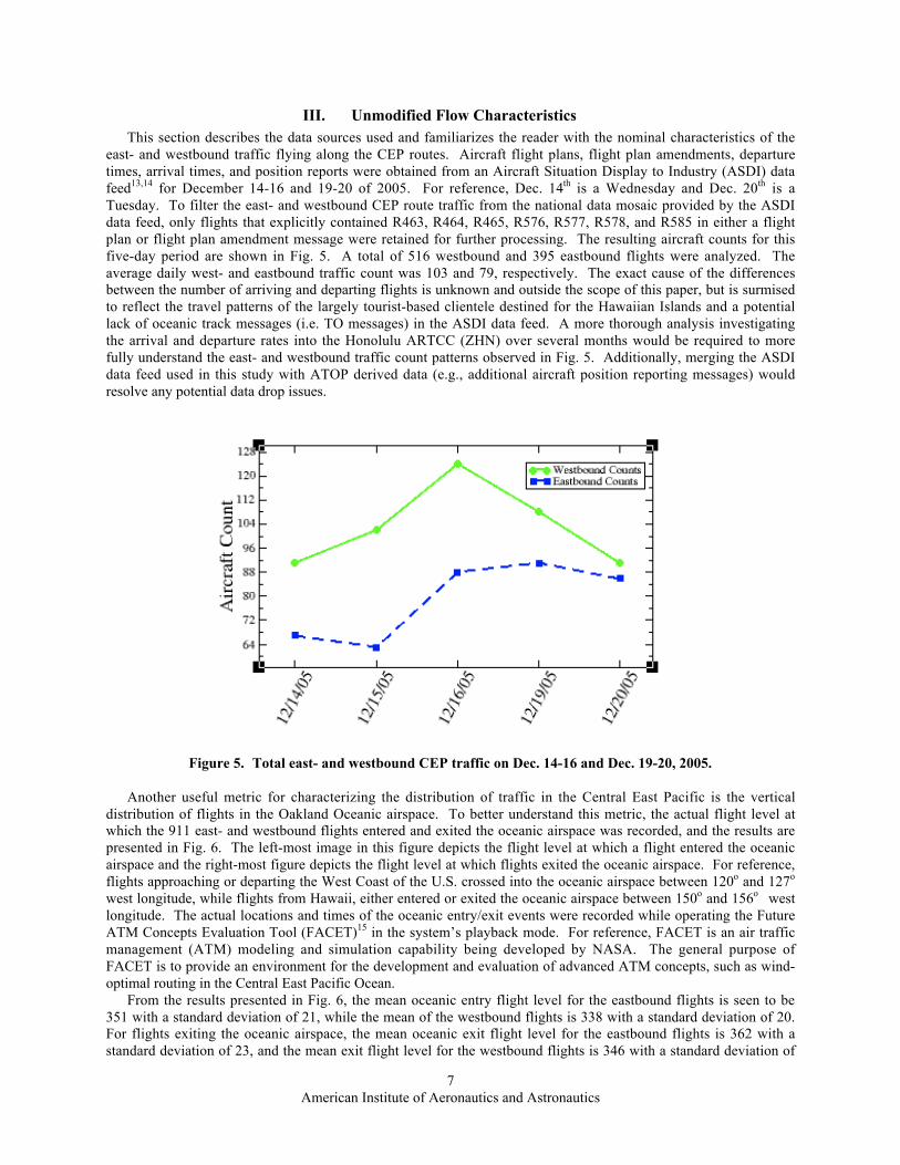
east- and westbound traffic flying along the CEP routes. Aircraft flight plans, flight plan amendments, departuretimes, arrival times, and position reports were obtained from an Aircraft Situation Display to Industry (ASDI) datafeed13,14 for December 14-16 and 19-20 of 2005. For reference, Dec. 14th is a Wednesday and Dec. 20th is aTuesday. To filter the east- and westbound CEP route traffic from the national data mosaic provided by the ASDIdata feed, only flights that explicitly contained R463, R464, R465, R576, R577, R578, and R585 in either a flightplan or flight plan amendment message were retained for further processing. The resulting aircraft counts for thisfive-day period are shown in Fig. 5. A total of 516 westbound and 395 eastbound flights were analyzed. Theaverage daily west- and eastbound traffic count was 103 and 79, respectively. The exact cause of the differencesbetween the number of arriving and departing flights is unknown and outside the scope of this paper, but is surmisedto reflect the travel patterns of the largely tourist-based clientele destined for the Hawaiian Islands and a potentiallack of oceanic track messages (i.e. TO messages) in the ASDI data feed. A more thorough analysis investigatingthe arrival and departure rates into the Honolulu ARTCC (ZHN) over several months would be required to morefully understand the east- and westbound traffic count patterns observed in Fig. 5. Additionally, merging the ASDIdata feed used in this study with ATOP derived data (e.g., additional aircraft position reporting messages) wouldresolve any potential data drop issues.

Figure 5. Total east- and westbound CEP traffic on Dec. 14-16 and Dec. 19-20, 2005.

Another useful metric for characterizing the distribution of traffic in the Central East Pacific is the verticaldistribution of flights in the Oakland Oceanic airspace. To better understand this metric, the actual flight level atwhich the 911 east- and westbound flights entered and exited the oceanic airspace was recorded, and the results arepresented in Fig. 6. The left-most image in this figure depicts the flight level at which a flight entered the oceanicairspace and the right-most figure depicts the flight level at which flights exited the oceanic airspace. For reference,flights approaching or departing the West Coast of the U.S. crossed into the oceanic airspace between 120o and 127o

west longitude, while flights from Hawaii, either entered or exited the oceanic airspace between 150o and 156o westlongitude. The actual locations and times of the oceanic entry/exit events were recorded while operating the FutureATM Concepts Evaluation Tool (FACET)15 in the system’s playback mode. For reference, FACET is an air trafficmanagement (ATM) modeling and simulation capability being developed by NASA. The general purpose ofFACET is to provide an environment for the development and evaluation of advanced ATM concepts, such as wind-optimal routing in the Central East Pacific Ocean.

From the results presented in Fig. 6, the mean oceanic entry flight level for the eastbound flights is seen to be351 with a standard deviation of 21, while the mean of the westbound flights is 338 with a standard deviation of 20.For flights exiting the oceanic airspace, the mean oceanic exit flight level for the eastbound flights is 362 with astandard deviation of 23, and the mean exit flight level for the westbound flights is 346 with a standard deviation of


23. Comparing the entry/exit flight levels for either the east- or westbound flights, one finds that the exit flight levelis on average higher than the entry flight level. Intuitively, this is the expected outcome, since an aircraft’s“optimal” flight level increases with decreasing weight.

Figure 6. Vertical distribution of the east- and westbound flights upon entering (left) and exiting (right) theOakland Oceanic Airspace.

Another key feature used to characterize the nominal flow of traffic was the temporal distribution of these flightsalong the fixed CEP route structure. This metric is useful for identifying arrival and departure pushes to and fromthe Hawaiian Islands. In Fig. 7, the oceanic entry and exit counts as a function of time are displayed for both theeastbound and westbound flights for the five days analyzed. Although minor deviations in the aircraft counts areobserved when comparing the data across multiple days, several prominent features can be extracted. Starting withthe eastbound oceanic entry counts (top-left), a small peak in the traffic counts is observed at 4:30 UTC followed bya larger peak at 10:00 UTC. Since flights departing HNL take approximately 45 minutes to enter the oceanicairspace, these two peaks correspond to eastbound Hawaiian flights that are departing at 5:45 pm and 11:15 pmHawaii-Aleutian Standard Time (HST), respectively. As the eastbound Hawaiian departures exit the oceanicairspace, these flights give rise to the aircraft counts that are shown in the top-right image of Fig. 7. This figureshows a cluster of flights exiting the oceanic airspace at around 7:30 UTC and a prominent peak near 13:00 UTC.Since flights departing Hawaii spend roughly 3 to 3.5 hours in the oceanic environment en route to the west coast ofthe U.S., these two features correspond to the aforementioned 5:45 pm and 11:15 pm HST departures exiting theoceanic airspace.

The last two images (bottom-left and bottom-right) in Fig. 7 correspond to the oceanic entry and exit aircraftcounts for the westbound flights. Beginning first with the oceanic entry counts, two broad features are observed.The first is a cluster around 2:00 UTC and the second more prominent feature that is clustered around 18:00 UTC.Since travel time from a west coast airport to the oceanic center boundary takes approximately 50 minutes (based onthe flight time from LAX), these two features correspond roughly to the 5:10 pm and 11:10 am Pacific StandardTime (PST) departure pushes from the west coast. As these flights cross the Central Pacific, they reemerge at theZHN boundary after approximately 3.5 hours of flight in oceanic airspace. The entry of these flights into ZHNairspace is evident in the bottom-right image in Fig. 7, where a cluster of flights crosses into ZHN at approximately5:30 UTC, while a second more prominent group of flights enters ZHN airspace at approximately 21:30 UTC.


Figure 7. Eastbound oceanic entry (top-left) and exit (top-right) counts and westbound oceanic entry(bottom-left) and exit (bottom-right) counts along the CEP routes.

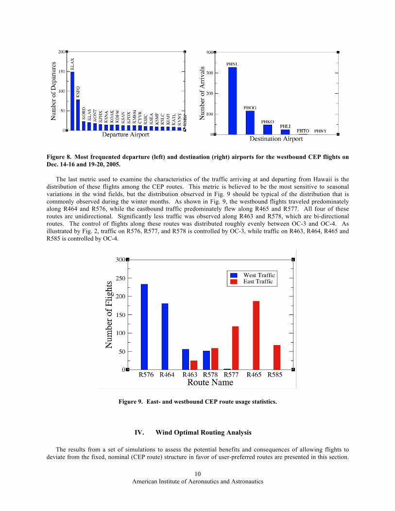
For the flights considered in this study, the total oceanic transit time is fairly constant and generally variesbetween 3 and 4 hours. The dispersion observed in the peaks in Fig. 7 therefore is more strongly influenced by thedestination airport and the airline’s schedules than the total time spent traveling in the oceanic environment. To gainmore insight into the origin and destination airports that are frequented by flights on the CEP routes, Fig. 8 containsdeparture airport usage statistics (left image) and arrival airport usage statistics (right image) for the westbound CEPflights.

For the departure statistics, only the top 21 airports are illustrated, although flights were observed to depart from41 airports during the five-day period analyzed. Roughly 44% of all westbound flights departed from Los AngelesInternational Airport, KLAX, and San Francisco International Airport, KSFO. The names associated with theremaining departure airport acronyms in Fig. 8 follow: Chicago O’Hare (KORD), McCarran Intl. (KLAS), OntarioIntl. (KONT), Phoenix Sky Harbor Intl. (KPHX), John Wayne Airport (KSNA), Oakland Metropolitan Intl.(KOAK), Dallas/Fort Worth Intl. (KDFW), San Diego Intl. (KSAN), Portland Intl. (KPDX), Memphis Intl.(KMEM), Vancouver Intl. (CYVR), Norman Y. Mineta San Jose Intl. (KSJC), Seattle-Tacoma Intl. (KSEA),Sacramento Intl. (KSMF), Salt Lake City Intl. (KSLC), Houston Intl. (KIAH), Atlanta Intl. (KATL), Van Nuys(KVNY), and Minneapolis-St. Paul Intl. (KMSP).

The arrival airport statistics in the rightmost image of Fig. 8, illustrate that approximately 63% of all flightsdestined for Hawaii landed at Honolulu Intl. Airport (PHNL). In contrast, only one flight landed at Lanai (PHNY)and two flights landed at Hilo (PHTO) during the same five-day period. Of the remaining flights, 22% landed atKahului (PHOG), 9% landed at Kona/Keahole Kailua (PHKO), and 5% landed at Lihue/Kauai Island (PHLI).


Figure 8. Most frequented departure (left) and destination (right) airports for the westbound CEP flights onDec. 14-16 and 19-20, 2005.

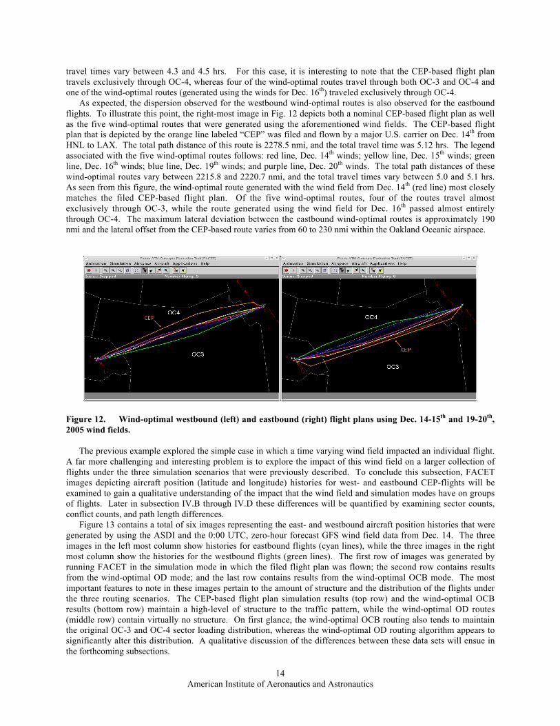
The last metric used to examine the characteristics of the traffic arriving at and departing from Hawaii is thedistribution of these flights among the CEP routes. This metric is believed to be the most sensitive to seasonalvariations in the wind fields, but the distribution observed in Fig. 9 should be typical of the distribution that iscommonly observed during the winter months. As shown in Fig. 9, the westbound flights traveled predominatelyalong R464 and R576, while the eastbound traffic predominately flew along R465 and R577. All four of theseroutes are unidirectional. Significantly less traffic was observed along R463 and R578, which are bi-directionalroutes. The control of flights along these routes was distributed roughly evenly between OC-3 and OC-4. Asillustrated by Fig. 2, traffic on R576, R577, and R578 is controlled by OC-3, while traffic on R463, R464, R465 andR585 is controlled by OC-4.

Figure 9. East- and westbound CEP route usage statistics.

IV. Wind Optimal Routing Analysis

The results from a set of simulations to assess the potential benefits and consequences of allowing flights todeviate from the fixed, nominal (CEP route) structure in favor of user-preferred routes are presented in this section.


Using the ASDI data files and the wind fields from the Global Forecast System (GFS) Atmospheric Model16 forDec. 14-16 and 19-20 of 2005, three sets of simulations were run in FACET. In the first set of simulations, flightstraveled along their filed flight plans, as specified in the ASDI files. For the second set of simulations wind-optimaltrajectories were generated roughly within the oceanic center boundary (OCB), while in the third set of simulations awind-optimal trajectory was generated from the flight’s origin to the destination (OD).

The first set of simulations was designed to serve as a surrogate for current day routing options. FACET couldhave been operated in a playback mode in which the actual aircraft position reports from ASDI would have beenprocessed, as was done in Section III, but later comparisons between the playback results and the wind-optimalresults would have included not only the routing differences but also any aircraft performance modeling differencesas well. To generate the results for the second set of simulations (i.e. the OCB wind-optimal results), routegeneration began at the first waypoint prior to entering one of the CEP routes and ended after the first waypointimmediately following the last CEP route appearing in the nominal flight plan.

The remainder of this section is structured as follows. In subsection IV.A, the modified traffic patterncharacteristics are examined for the three simulations. To assess the potential impact that the wind-optimal routesmight have on the air traffic service provider, the sector count differences and first-loss-of-separation statistics arepresented in subsection IV.B and IV.C, respectively. These metrics are being presented because significantincreases in either of these values may substantially increase controller workload. Finally, the time- and distance-savings statistics for both wind-optimal routing simulations are presented in subsection IV.D.

A. Traffic PatternsIn this section, the individual and aggregate traffic pattern characteristics are examined for flights on both the

nominal CEP-based routes and the two wind-optimal routes. As an example of these different routing scenarios,consider the three routes between ORD and HNL in Fig. 10. The solid green route that is labeled “CEP” in thisfigure is the nominal flight plan that was filed by a major U.S. air carrier on Dec. 14, 2005 between this city pair.The solid magenta line labeled “OCB” is the corresponding OCB wind-optimal route for this flight. In calculatingthis route, route generation began at the “BEBOP” fix, which lies near the ZOA-OAO boundary, and continued upto the “BITTA” fix, which lies near the OAO-ZHN boundary. Finally, the red line in this figure that is labeled“OD” depicts the wind-optimal route that was generated between ORD and HNL. As expected, the amount ofvariance between the “CEP” and “OD” routes is significantly larger than the variance between the “OCB” and“CEP” routes.

Figure 10. Fixed versus wind-optimal routes between ORD and HNL.

Since the magnitude and direction of the winds that were used have such a significant impact on the results, abrief discussion regarding the coverage and characteristics of the National Oceanic and Atmospheric Administration


(NOAA) atmospheric model is appropriate. GFS is a global atmospheric model with a horizontal resolution ofapproximately 0.5o x 0.5o latitude/longitude and an unequally spaced vertical resolution starting at 1000 mb(surface) and extending up to 100 mb. Updates to the GFS model are available every six hours and forecasts areavailable up to 16 days into the future. As an example of the wind fields that were used, the 00:00 UTC, zero hourforecast wind magnitude contours at 250 mb., which roughly encompasses flight levels 310 through 360 over theCentral East Pacific, are shown in Fig. 11. The top-left image in this figure contains the contours for Dec. 14th, thetop-right image shows the Dec. 15th data, the middle-left image shows the Dec. 16th data, the middle-right imageshows the Dec. 19th data, and finally the bottom image shows the contours for Dec. 20th. The legend associated withthe wind magnitude contours follows: > 120 kts., magenta; >105 kts., red; >90 kts. orange; >75 kts., yellow; >60kts., light green; >45 kts., dark green; >30 kts, light blue; >15 kts, blue; and >0 kts, dark blue. Although thedirection of the wind field is not illustrated in these images, the winds are generally westerly (i.e., flowing west toeast) in this region of the Pacific Ocean. For reference, the Hawaiian Islands are shown at the bottom left of eachimage in Fig. 11 and the west coast of the United States is shown on the right side of each image. A region of verystrong, westerly winds (>120 kts.) is shown in each of these figures and the location of these strong winds tended tomove in a northerly direction during the five day period that was examined in this study. As expected, the variablewind fields illustrated in Fig. 11 had a significant impact on the wind-optimal routes and will now be explored inmore detail.

The band of strong winds (>100 kts) that is exhibited in Fig. 11 is most likely the polar jet stream17 that is oftenlocated in this region during the winter. The westerly winds within the core of this jet stream often exceed 100 kts.,as illustrated, and can reach speeds as high as 250 kts. During the summer months, this jet stream tends to weakenand move farther north towards Canada. Since the results of the wind-optimal routing algorithm are, by nature,susceptible to the magnitude and direction of the wind field in which the routing is being performed, the results inthis study should represent an upper bound on the maximum savings and impact that can be expected in this regionof the ocean. A follow-on study that that examines the seasonal savings and impact of wind-optimal routing in thePacific Ocean would be beneficial.


Figure 11. GFS wind contours at 250 mb for Dec. 14th (top-left), Dec. 15th (top-right), Dec. 16th (middle-left), Dec. 19th (middle-right), and Dec. 20th (bottom) in the Central East Pacific.

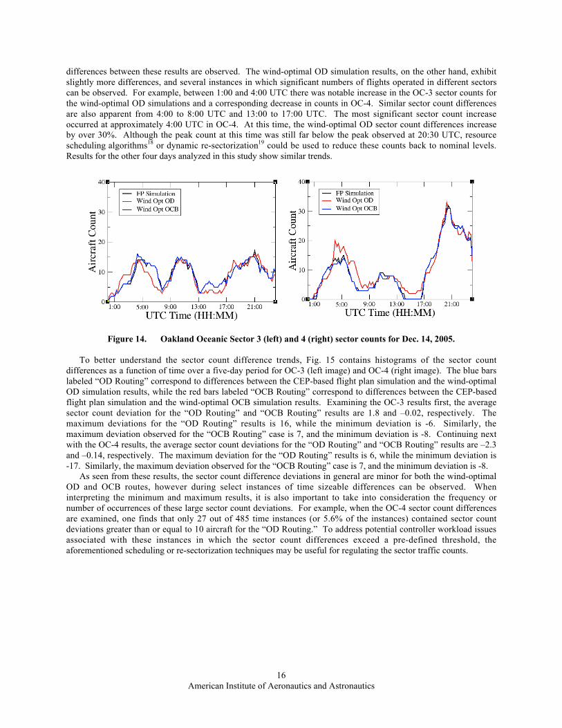
To illustrate the impact that the varying wind fields can have on an individual flight, consider the flight plansdepicted in Fig. 12. The nominal, westbound flight plan, which is represented by the orange line labeled “CEP,”was filed and flown by a major U.S. carrier on Dec. 14, 2005. The total path distance of this route is 2,305 nmi andthe total travel time is 4.52 hrs. The corresponding westbound wind-optimal routes that were generated directlyfrom LAX to HNL using the wind fields illustrated in Fig. 11 are also shown in this image and drawn as follows: redline, Dec. 14th winds; yellow line, Dec. 15th winds; green line, Dec. 16th winds; blue line, Dec. 19th winds; and purpleline, Dec. 20th winds. The maximum lateral spread between the westbound wind-optimal routes is 130 nmi and themaximum lateral offset from the westbound CEP-based flight plan route in the oceanic center varies from 120 to260 nmi. The total path distance of these wind-optimal routes varies between 2218 and 2226 nmi, and the total


travel times vary between 4.3 and 4.5 hrs. For this case, it is interesting to note that the CEP-based flight plantravels exclusively through OC-4, whereas four of the wind-optimal routes travel through both OC-3 and OC-4 andone of the wind-optimal routes (generated using the winds for Dec. 16th) traveled exclusively through OC-4.

As expected, the dispersion observed for the westbound wind-optimal routes is also observed for the eastboundflights. To illustrate this point, the right-most image in Fig. 12 depicts both a nominal CEP-based flight plan as wellas the five wind-optimal routes that were generated using the aforementioned wind fields. The CEP-based flightplan that is depicted by the orange line labeled “CEP” was filed and flown by a major U.S. carrier on Dec. 14th fromHNL to LAX. The total path distance of this route is 2278.5 nmi, and the total travel time was 5.12 hrs. The legendassociated with the five wind-optimal routes follows: red line, Dec. 14th winds; yellow line, Dec. 15th winds; greenline, Dec. 16th winds; blue line, Dec. 19th winds; and purple line, Dec. 20th winds. The total path distances of thesewind-optimal routes vary between 2215.8 and 2220.7 nmi, and the total travel times vary between 5.0 and 5.1 hrs.As seen from this figure, the wind-optimal route generated with the wind field from Dec. 14th (red line) most closelymatches the filed CEP-based flight plan. Of the five wind-optimal routes, four of the routes travel almostexclusively through OC-3, while the route generated using the wind field for Dec. 16th passed almost entirelythrough OC-4. The maximum lateral deviation between the eastbound wind-optimal routes is approximately 190nmi and the lateral offset from the CEP-based route varies from 60 to 230 nmi within the Oakland Oceanic airspace.

Figure 12. Wind-optimal westbound (left) and eastbound (right) flight plans using Dec. 14-15th and 19-20th,2005 wind fields.

The previous example explored the simple case in which a time varying wind field impacted an individual flight.A far more challenging and interesting problem is to explore the impact of this wind field on a larger collection offlights under the three simulation scenarios that were previously described. To conclude this subsection, FACETimages depicting aircraft position (latitude and longitude) histories for west- and eastbound CEP-flights will beexamined to gain a qualitative understanding of the impact that the wind field and simulation modes have on groupsof flights. Later in subsection IV.B through IV.D these differences will be quantified by examining sector counts,conflict counts, and path length differences.

Figure 13 contains a total of six images representing the east- and westbound aircraft position histories that weregenerated by using the ASDI and the 0:00 UTC, zero-hour forecast GFS wind field data from Dec. 14. The threeimages in the left most column show histories for eastbound flights (cyan lines), while the three images in the rightmost column show the histories for the westbound flights (green lines). The first row of images was generated byrunning FACET in the simulation mode in which the filed flight plan was flown; the second row contains resultsfrom the wind-optimal OD mode; and the last row contains results from the wind-optimal OCB mode. The mostimportant features to note in these images pertain to the amount of structure and the distribution of the flights underthe three routing scenarios. The CEP-based flight plan simulation results (top row) and the wind-optimal OCBresults (bottom row) maintain a high-level of structure to the traffic pattern, while the wind-optimal OD routes(middle row) contain virtually no structure. On first glance, the wind-optimal OCB routing also tends to maintainthe original OC-3 and OC-4 sector loading distribution, whereas the wind-optimal OD routing algorithm appears tosignificantly alter this distribution. A qualitative discussion of the differences between these data sets will ensue inthe forthcoming subsections.


Figure 13. Flight Histories for Dec. 14, 2006 for eastbound, nominal (CEP) routes (top-left), westboundnominal (CEP) routes (top-right), eastbound OD routes (mid-left), westbound OD routes (mid-right),eastbound OCB routes (bottom-left), and westbound OCB routes (bottom-right).

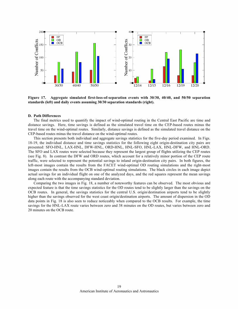
B. Sector CountsTo quantify the impact that wind-optimal routing can have on the airspace, this section contains both detailed

sector count differences for Dec. 14th and aggregate sector count differences for the five-day period. Beginning firstwith the detailed sector count differences shown in Fig. 14, several features are worth noting. The left-most imagein this figure contains the OC-3 sector counts as a function of time, and the right-most image contains the OC-4sector counts. In each image, three different curves are presented that represent the number of unique flightsobserved in a 15-minute period as a function of time. The black curve labeled “FP Simulation” contains the countsresulting from operating FACET in the simulation mode in which aircraft followed their CEP-based flight planroutes, the red line corresponds to the counts when FACET is operated in the wind-optimal OD mode, and finallythe blue line corresponds to the results from a FACET wind-optimal OCB simulation. As expected, both the CEP-based flight plan simulation results and the wind-optimal OCB results are in good agreement, and only minor


differences between these results are observed. The wind-optimal OD simulation results, on the other hand, exhibitslightly more differences, and several instances in which significant numbers of flights operated in different sectorscan be observed. For example, between 1:00 and 4:00 UTC there was notable increase in the OC-3 sector counts forthe wind-optimal OD simulations and a corresponding decrease in counts in OC-4. Similar sector count differencesare also apparent from 4:00 to 8:00 UTC and 13:00 to 17:00 UTC. The most significant sector count increaseoccurred at approximately 4:00 UTC in OC-4. At this time, the wind-optimal OD sector count differences increaseby over 30%. Although the peak count at this time was still far below the peak observed at 20:30 UTC, resourcescheduling algorithms18 or dynamic re-sectorization19 could be used to reduce these counts back to nominal levels.Results for the other four days analyzed in this study show similar trends.

Figure 14. Oakland Oceanic Sector 3 (left) and 4 (right) sector counts for Dec. 14, 2005.

To better understand the sector count difference trends, Fig. 15 contains histograms of the sector countdifferences as a function of time over a five-day period for OC-3 (left image) and OC-4 (right image). The blue barslabeled “OD Routing” correspond to differences between the CEP-based flight plan simulation and the wind-optimalOD simulation results, while the red bars labeled “OCB Routing” correspond to differences between the CEP-basedflight plan simulation and the wind-optimal OCB simulation results. Examining the OC-3 results first, the averagesector count deviation for the “OD Routing” and “OCB Routing” results are 1.8 and –0.02, respectively. Themaximum deviations for the “OD Routing” results is 16, while the minimum deviation is -6. Similarly, themaximum deviation observed for the “OCB Routing” case is 7, and the minimum deviation is -8. Continuing nextwith the OC-4 results, the average sector count deviations for the “OD Routing” and “OCB Routing” results are –2.3and –0.14, respectively. The maximum deviation for the “OD Routing” results is 6, while the minimum deviation is-17. Similarly, the maximum deviation observed for the “OCB Routing” case is 7, and the minimum deviation is -8.

As seen from these results, the sector count difference deviations in general are minor for both the wind-optimalOD and OCB routes, however during select instances of time sizeable differences can be observed. Wheninterpreting the minimum and maximum results, it is also important to take into consideration the frequency ornumber of occurrences of these large sector count deviations. For example, when the OC-4 sector count differencesare examined, one finds that only 27 out of 485 time instances (or 5.6% of the instances) contained sector countdeviations greater than or equal to 10 aircraft for the “OD Routing.” To address potential controller workload issuesassociated with these instances in which the sector count differences exceed a pre-defined threshold, theaforementioned scheduling or re-sectorization techniques may be useful for regulating the sector traffic counts.


Figure 15. Aggregate Oakland Oceanic Sector 3 (left) and 4 (right) sector count differences.

C. First-Loss-of-Separation StatisticsChanges in the traffic patterns in the Central East Pacific cannot only increase the workload of a controller but

can also give rise to an increase in the number of possible losses of separation. With the deployment of the newATOP system, the FAA is proposing to reduce the separation standards on the CEP routes to 30 nmi lateral spacing,30 nmi longitudinal spacing, and 1000 ft vertical separation. Using FACET, the simulated trajectories for all east-and westbound flights were examined for possible losses of separation on both the nominal CEP-based flight planroutes, the OD wind-optimal routes, and the OCB wind-optimal routes using these reduced separation standards andtwo additional sets of more restrictive standards. As previously mentioned, the separation standards for flights onthe CEP routes are as follows:2

o 1,000 feet vertical separationo 50 nmi lateral separationo 5-10 min longitudinal separation using the “Mach Number Technique” that depends on differences in

the Mach number between aircraft pairsSince the primary focus of this study was on developing and assessing the impact of wind-optimal routes, and

not on developing a conflict probe for Oakland Oceanic airspace, a decision was made to greatly simplify thedefinition of a first-loss-of-separation (FLOS) event in this study. Therefore, losses of separation were identifiedunder the following three different separation criteria: (1) 30 nmi lateral spacing, 30 nmi longitudinal spacing, and1000 ft vertical spacing; (2) 40 nmi lateral spacing, 40 nmi longitudinal spacing, and 1000 ft vertical spacing; and(3) 50 nmi lateral spacing, 50 nmi longitudinal spacing, and 1000 ft vertical spacing. For the remainder of thissection, the first of these three separation standards will be referred to as the “30/30” separation standard, the secondwill be referred to as the “40/40” separation standards, and the last of these three will be referred to as the “50/50”separation standard. Both the lateral and longitudinal separation standards for the 30/30 cases are less restrictivethan current standards. For the 40/40 cases, the lateral separation standards are less than current standards, as are thelongitudinal separation standards, except when the Mach number of the leading aircraft is greater thanapproximately Mach 0.05 faster than the trailing aircraft. Finally, for the 50/50 cases, the lateral separationstandards are the same as current day standards, and the longitudinal standards are less restrictive when the Machnumber of the leading aircraft is greater than approximately Mach 0.04 faster than the trailing aircraft.2

For the remainder of this section, FLOS statistics will be presented for both a single day and aggregated over afive-day period. The geographical location for each unique, simulated FLOS event that occurred using the Dec. 16th

data set is presented in Fig. 16 using both the 30/30 (left image) and the 50/50 (right image) separation standards.The red circles in both images depict the unique FLOS locations generated with the CEP-based flight plansimulations, the green squares depict the location generated with the OD wind-optimal routing, and lastly the bluetriangles depict the locations resulting from the OCB wind-optimal routing simulation. For the 30/30 cases, therewere 13 FLOS events for the CEP-based flight plan simulation results, 24 FLOS events for the OD wind-optimalrouting simulation, and 19 FLOS events for the OCB wind-optimal routing simulation. Similarly, for the 50/50cases, 17 FLOS events were observed for the CEP-based flight plan simulation, 48 FLOS events were observed forthe OD wind-optimal routing case, and 31 FLOS events were generated for the OCB wind-optimal routing case.


It is also important to note that the FLOS events depicted in Fig. 16 take place at a wide range of flight levels.For example for the 17 FLOS events associated with the CEP-based flight plan simulations, events were observed atsix different flight levels ranging from 320 through 370. With regard to the geographical location of the FLOSevents depicted in this figure, there were numerous events near the oceanic center boundary, which presumablywould never have occurred if the planes had passed from the Center airspace (e.g. ZHN and ZOA) into the oceanicairspace properly spaced. Recall that the separation standard in the Center airspace is only five nmi in the lateraland longitudinal domain and 1,000 ft in the vertical domain. This refinement would be beneficial to study in moredetail as part of a future study. Another feature to note is the large number of FLOS events, especially for the ODwind-optimal simulation case, that occur at the boundary between OC-3 and OC-4. A large number of these eventsare associated with the westbound traffic streams that were observed to converge on this day at the boundary (seethe middle images in Fig. 13 for example).

Figure 16. Simulated first-loss-of-separation locations using 30/30 (left) and 50/50 (right)latitudinal/longitudinal separation standards for Dec. 16, 2005

To begin understanding the potential long-term implications of reducing the separation standards in the CentralEast Pacific, aggregate FLOS statistics are presented in Fig. 17. The left-most image in this figure contains theaggregate, five-day FLOS counts for the three different FACET simulations, assuming the following separationstandards: 30/30, 40/40, and 50/50. As expected, the number of FLOS events tends to increase with increasingseparation standards, and the rate of increase amongst the three different simulations is roughly equal. For allseparation standards, the OD wind-optimal routing results lead to the largest number of FLOS events, while theCEP-based simulation results lead to the least number of events. This is to be expected, since the OD wind-optimalroutes tend to allow streams of aircraft departing from different areas to converge, whereas the CEP-based routestend to isolate the predominant traffic streams traveling to and from Hawaii.

The second image in Fig. 17 contains the daily FLOS counts at each date for the three different FACETsimulations when the 30/30 separation standards are in place. Typically, the number of FLOS events associatedwith the CEP-based routing is lower than the other simulation results, and the OD wind-optimal simulation resultstend to yield the most number of FLOS events. The total number of FLOS events also tends to track the totalaircraft counts that are displayed in Fig. 5. For example, the lowest aircraft and FLOS counts occurred on Dec. 14th,while the highest aircraft and FLOS counts occurred on Dec. 16th. Based on the results presented in this study, thenumber of FLOS events would significantly increase when transitioning from the nominal (CEP-based) routes toeither the wind-optimal OD or OCB routes, which in turn could increase the workload of a controller handling theseflights. A follow-on study that explores the use of additional control mechanisms, such as departure or speedcontrols, is required to determine if the number of FLOS events for the wind-optimal routes can be reduced to theCEP-routing levels.


Figure 17. Aggregate simulated first-loss-of-separation events with 30/30, 40/40, and 50/50 separationstandards (left) and daily events assuming 30/30 separation standards (right).

D. Path DifferencesThe final metrics used to quantify the impact of wind-optimal routing in the Central East Pacific are time and

distance savings. Here, time savings is defined as the simulated travel time on the CEP-based routes minus thetravel time on the wind-optimal routes. Similarly, distance savings is defined as the simulated travel distance on theCEP-based routes minus the travel distance on the wind-optimal routes.

This section presents both individual and aggregate savings statistics for the five-day period examined. In Figs.18-19, the individual distance and time savings statistics for the following eight origin-destination city pairs arepresented: SFO-HNL, LAX-HNL, DFW-HNL, ORD-HNL, HNL-SFO, HNL-LAX, HNL-DFW, and HNL-ORD.The SFO and LAX routes were selected because they represent the largest group of flights utilizing the CEP routes(see Fig. 8). In contrast the DFW and ORD routes, which account for a relatively minor portion of the CEP routetraffic, were selected to represent the potential savings to inland origin-destination city pairs. In both figures, theleft-most images contain the results from the FACET wind-optimal OD routing simulations and the right-mostimages contain the results from the OCB wind-optimal routing simulations. The black circles in each image depictactual savings for an individual flight on one of the analyzed days, and the red squares represent the mean savingsalong each route with the accompanying standard deviation.

Comparing the two images in Fig. 18, a number of noteworthy features can be observed. The most obvious andexpected feature is that the time savings statistics for the OD routes tend to be slightly larger than the savings on theOCB routes. In general, the savings statistics for the central U.S. origin/destination airports tend to be slightlyhigher than the savings observed for the west coast origin/destination airports. The amount of dispersion in the ODdata points in Fig. 18 is also seen to reduce noticeably when compared to the OCB results. For example, the timesavings for the HNL-LAX route varies between zero and 38 minutes on the OD routes, but varies between zero and20 minutes on the OCB route.


Figure 18. Wind-optimal OD (left) and OCB (right) time savings statistics for select origin-destinationairport pairs

Continuing with the individual distance savings statistics that are presented in Fig. 19, a number of trends thattend to mirror the results in Fig. 18 are observed. The most notable difference between the between the OD (leftimage) and OCB (right image) wind-optimal routing results is the extent to which the data dispersion is reduced inthe OCB simulations. For example, the distance savings results varied between 196 nmi and –16 nmi for flightstraveling between SFO and HNL under the OD simulations, but the variance was only between 51 nmi and –17 nmifor the OCB results. It is worth noting that the large distance deviations (>170 nmi) that were observed for the SFOto HNL flights all occurred when using the data sets for Dec. 19th. As can be seen from the wind fields that aredepicted in Fig. 11, a very strong (>120 kt) head wind existed in much of sector OC-4 on this day. In all four casesin which distance savings greater than 170 nmi were recorded, the filed flight plan routed the plane on a southerlyroute through OC-3, whereas the OCB wind-optimal route flew the plane on a more direct route through OC-4.Finally, a general trend can also be observed for the OD simulations in which the distance savings is greater forinland origin/destination airports (e.g. DFW and ORD) than it is for origin/destination airports on the west coast (e.gSFO and LAX). As expected, this trend does not hold true for the OCB simulations, since wind-optimal routing isnot initiated until the flight reaches the oceanic center boundary.

Figure 19. Wind-optimal OD (left) and OCB (right) distance savings statistics for select origin-destinationairport pairs

Aggregate time and distance saving statistics for all origin-destination pairs over the five-day period examinedare presented in Figs. 20 and 21. The left most image in each of these figures depicts the differences between theflight plan and OD wind-optimal routing simulations, while the right most image depicts differences between theflight plan and OCB wind-optimal routing simulations. Thirty-one time bins ranging from zero minutes of savings


to 30 minutes of savings in increments of one minute were used to classify the data appearing in Fig. 20. Theaverage time savings for the OD simulations was 9.9 min with a standard deviation of 7.3 min, while the averagetime savings for the OCB simulations was 4.8 min with a standard deviation of 5.0 min. For reference, the averagetravel time on the nominal (CEP-based) routes over the five-days was 5.5 hrs.

A number of interesting trends are evident in the two images appearing in Fig. 20. Firstly, the time savingsstatistics are strongly attenuated for the OCB simulations, while the OD simulation results exhibit a large tail. Inregards to the significant number of flights with time savings of 30 minutes, over half of these flights occurred withthe Dec. 19th data set and could be attributed to significant differences between the filed flight plan route and thecalculated wind-optimal routes. For example, in most instances flights filed through OC-4 encountered a significanthead wind, while a more southerly wind-optimal route was available. These very large time savings are by nomeans the norm and can only be expected when (1) the polar jet stream traverses OC-3 or OC-4 and (2) the aircarrier does not compensate for the prevailing wind patterns. Interestingly enough, a sizeable number of the flightswith very large time savings were general aviation (GA) flights, which may not have as sophisticated routingsoftware as the major air carriers servicing this market.

Figure 20. Aggregate wind-optimal time saving statistics for OD routing (left) and OCB routing (right)

The aggregate, five-day distance savings statistics for both the OD (left-image) and the OCB (right-image) wind-optimal routing simulations are presented in Fig. 21. Twenty-four distance bins ranging from –30 nmi to 200 nmi insteps of 10 nmi were used in creating the histograms in these figures. The average distance savings for the ODsimulations was 36 nmi with a standard deviation of 42 nmi, while the average savings for the OCB simulations was4 nmi with a standard deviation of 29 nmi. For reference, the average travel distance on the nominal (CEP-based)routes over the five-days was 2,401 nmi. The most striking difference between these two figures is the variability ofthe distance savings results. As previously mentioned, this is to be expected given the fact that the OD wind-optimalrouting simulations provide each flight with significantly more routing variability than is provided to flights underthe OCB wind-optimal routing simulations. The flights with very large distance savings (>150 nmi) are the sameflights that were previously discussed in which large variations in the filed and wind-optimal routes were observed.


Figure 21. Aggregate wind-optimal distance saving statistics for OD routing (left) and OCB routing (right)

.

V. Concluding RemarksThis paper contains the results of the first extensive study designed to characterize the flow of traffic on the CEP

routes and to assess the potential benefits of transitioning from these fixed routes to user-preferred routes. As asurrogate for the actual user-preferred routes, a minimum-time, wind-optimal dynamic programming algorithm wasdeveloped and utilized in this study. The results of this study are important because with the introduction of theFAA’s new ATOP system at Oakland Center, increased route flexibility and reduced separation standards canpotentially now be accommodated, which can translate directly into increased revenue for the airlines.

The characterization of the traffic patterns on the CEP routes was accomplished by first operating NASA’sFACET in playback mode with 120 hrs. of the FAA’s ASDI data from December 14-16 and 19-20. From this dataset, 911 east- and westbound flights were identified that utilized at least one of the seven CEP routes. Using a suiteof newly developed analysis capabilities, the following metrics were calculated: flight level usage, temporal flightdistribution, CEP route usage, and origin-destination distribution.

Following the characterization of the nominal traffic patterns on the CEP routes, the results of a comprehensiveinvestigation of the potential benefits associated with transitioning from the fixed CEP based routes to user-preferredroutes were presented. To accomplish this task, the aforementioned wind-optimal dynamic programming algorithmwas implemented in FACET, and 15, 24-hour simulations were conducted with the modified system. Of thesesimulations, five routed flights on the nominal (CEP-based) routes, five routed flights between the origin anddestination on wind-optimal trajectories (OD), and the remaining five routed flights on nominal trajectories in thenon-oceanic domain and wind-optimal trajectories in the oceanic domain (OCB).

The results of these 15, 24-hour simulations were characterized in terms sector count deviations, first loss ofseparation events, time savings, and distance savings. In general, only minor differences were found whencomparing the nominal sector counts with the counts resulting from the wind-optimal simulations. This issignificant, since the number of aircraft in a sector contributes significantly to the workload of a controller. Incontrast, the number of simulated first-loss-of-separation events was found to dramatically increase in the wind-optimal simulations. To reduce the number of these events to an acceptable level, research into additional controlstrategies, such as departure control, should be investigated. Finally, the average time savings for the OD and OCBwind-optimal routing simulations was found to be 9.9 min and 4.8 min, respectively, while the average distancesavings was found to be 36 nmi and 4.0 nmi, respectively.

In conclusion, wind-optimal routes offer a clear advantage over nominal (CEP-based) routes for the airspaceusers in the Central East Pacific, and research into new control strategies is essential for alleviating workload issuesassociated with this alternative routing strategy.


AppendixFor the current study, the incremental cost associated with transitioning between two successive states,

€

xk , and,

€

xk+1, is equal to the travel time between these two states. If the initial latitude/longitude position is denoted by

€

λ i ,τ i( ) and the final position is denoted by

€

λ f ,τ f( ) then the cost/travel time is given by20

€

C xk ,uk ,k( ) = t = d /Vg (15)

where

€

d = Rearth ⋅ cos−1 sinλ i ⋅sinλ f + cos(τ f −τ i) ⋅ cosλ i ⋅ cosλ f[ ] (16)

and

€

Vg = ˙ x 2 + ˙ y 2 (17)

Here

€

Rearth is the radius of the Earth, which is taken to be 3,444.046647 nm, and the horizontal components of thevelocity are denoted by

€

˙ x and

€

˙ y . These velocity components are calculated from the horizontal velocity of the

aircraft,

€

vh , the horizontal component of the wind velocity,

€

wh , the aircraft’s commanded heading,

€

χ com , and thehorizontal wind direction,

€

χh , using the following expressions:

€

˙ x = vh ⋅ cosχ com + wh ⋅ cos χh (18)

and

€

˙ y = vh ⋅sinχ com − wh ⋅sinχh (19)

The aircraft’s command heading,

€

χ com , is related the course angle for great circle navigation,

€

χGC , via thefollowing expression:

€

χ com = χGC − sin−1 wh vh( ) ⋅sin(χh − χGC )( ) (20)

where

€

χGC = tan−1sin(τ f −τ i) ⋅ cosλ f

sinλ f ⋅ cos λ i − sinλ i ⋅ cos λ f ⋅ cos(λ f − λ i)

(21)

AcknowledgmentsThe authors would like to acknowledge the help of Mr. Kevin Chamness and Mr. David M. Maynard from the

Federal Aviation Administration for providing the oceanic domain knowledge expertise required to complete thisstudy. The assistance of Dr. Parimal Kopardekar from NASA Ames Research Center and Mrs. Almira Williamsfrom CSSC, Inc. is also acknowledged for contributing to our understanding of flight routing and air trafficprocedures in the Pacific Ocean.

References

1Wu, Y. S., Karakis, T., and Merkle, M., “Performance Metrics for Oceanic Air Traffic Management,” Air Traffic ControlQuarterly, Vol. 12, No. 4, 2004, pp. 315-338.

2”Air Traffic Control,” Order 7110.65R, Federal Aviation Administration, Feb. 16, 2006.


3“Advanced Technologies & Oceanic Procedures (ATOP),” U.S. Dept. of Transportation, Federal Aviation Administration,URL: http://www.faa.gov/airports_airtraffic/technology/atop

4Nolan, M., Fundamentals of Air Traffic Control, 4th ed., Thomson Brooks/Cole, Belmont, CA, pp. 467-4705”Notice of Required Navigation Performance 10 (RNP-10) Implementation in the Oakland Center FIR,” Oakland NOTAM

A4335/98, Federal Aviation Administration, 1998.6Erzberger, H. and Lee, H., “Constrained Optimum Trajectories with Specified Range,” AIAA Journal of Guidance,

Navigation and Control, Vol. 3, Jan-Feb, 1980, pp. 78-85.7Jardin, M., “Real-Time Conflict Free Trajectory Optimization,” 5th USA/Europe ATM 2003 R&D Seminar, Budapest,

Hungary, June 23-27, 2005.8Bertsimas, D. and Patterson, S. S., “The Traffic Flow Management Rerouting Problem in Air Traffic Control: A Dynamic

Network Flow Approach,” Transportation Science, Vol. 34, No. 3, August 2000.9Barnhart, C., Boland, N. L., Clarke, L. W., Johnson, G. L., Nemhauser, and G. L., Shenoi, R. G., “Flight String Models for

Aircraft Fleeting and Routing,” Transportation Sciences, Vol. 32, Issue 3, March 1998.10Jardin, M., “Toward Real-Time En Route Air Traffic Control Optimization,” Ph.D. Dissertation, Stanford University, Dept.

of Aeronautics & Astronautics, April 2003.11Larson, R. E. and Casti, J. L., Principles of Dynamic Programming: Part 1 Basic Analytic and Computational Methods,

Marcel Dekker, Inc., 1978.12Williams, E., “Aviation Formulary, V1.42,” URL: http://williams.best.vwh.net/avform.htm.13“Enhanced Traffic Management System (ETMS),” Report No. VNTSC-DTS56-TMS-002, Volpe National Transportation

Center, U.S. Dept. of Transportation, Cambridge, MA, Oct. 2005.14“Aircraft Situation Display To Industry: Functional Description and Interface Control Document,” Report No. ASDI-FD-

001, Volpe National Transportation Center, U.S. Dept. of Transportation, Cambridge, MA, June 29, 2005.15Bilimoria, K., Sridhar, B., Chatterji, G. B., Sheth, K., and Grabbe, S., “FACET: Future ATM Concepts Evaluation Tool,”

Air Traffic Control Quarterly, Vol. 9, No. 1, 2001, pp. 1-20.16“EMC Model Documentation,” National Centers for Environmental Predictions, National Oceanic and Atmospheric

Administration, URL: http://www.emc.ncep.noaa.gov/modelinfo/.17Ahrens, C. D., Essentials of Meteorology: An Invitation to the Atmosphere, West Publishing Company, St. Paul, MN, 1993,

pp. 177-179.18Bertsimas, D., and Patterson S. S., “The Air Traffic Flow Management Problem with Enroute Capacities,” Operations

Research, Vol. 46, No. 3, May-June 1998, pp. 406-422.19Sridhar, B., Sheth, K. S., Grabbe, S., “Airspace Complexity and its Application in Air Traffic Management,” 2nd

USA/Europe Air Traffic Management R&D Seminar, Orlando, FL, Dec. 1-4, 1998.20Chatterji, G. B., Sridhar, B., and Bilimoria, K. D., “En-route Trajectory Prediction for Conflict Avoidance and Traffic

Management,” AIAA Guidance Navigation and Control Conference, San Diego, CA, July 29-31, 1996.

central east pacific flight routing - nasa

Documents