Central Limit TheoremBernoulli Trials

11/01/2005

Continuous Probability Densities

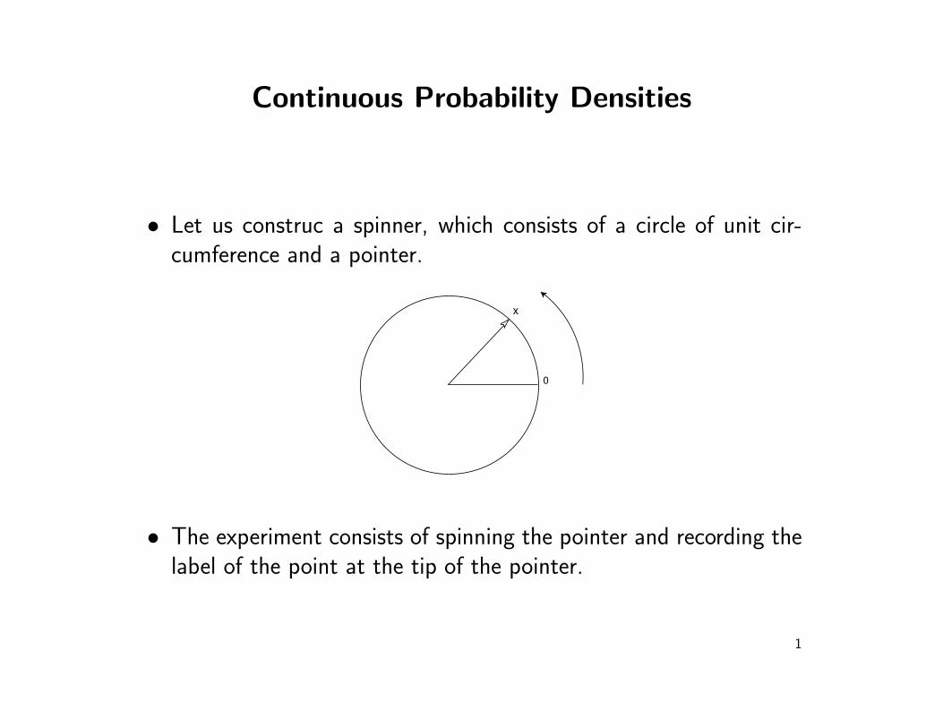
• Let us construc a spinner, which consists of a circle of unit cir-cumference and a pointer.

0

x

• The experiment consists of spinning the pointer and recording thelabel of the point at the tip of the pointer.

1

• We let the random variable X denote the value of this outcome.

• The sample space is clearly the interval [0, 1).

• It is necessary to assign the probability 0 to each outcome.

• The probabilityP (0 ≤ X ≤ 1)

should be equal to 1.

2

• We would like the equation

P (c ≤ X < d) = d− c

to be true for every choice of c and d.

• If we let E = [c, d], then we can write the above formula in theform

P (E) =∫

E

f(x) dx ,

where f(x) is the constant function with value 1.

3

Density Functions of Continuous RandomVariables

Let X be a continuous real-valued random variable. A densityfunction for X is a real-valued function f which satisfies

P (a ≤ X ≤ b) =∫ b

a

f(x) dx

for all a, b ∈ R.

4

• It is not the case that all continuous real-valued random variablespossess density functions.

• In terms of the density f(x), if E is a subset of R, then

P (X ∈ E) =∫

E

f(x) dx .

5

Example

• In the spinner experiment, we choose for our set of outcomes theinterval 0 ≤ x < 1, and for our density function

f(x) ={

1, if 0 ≤ x < 1,0, otherwise.

• If E is the event that the head of the spinner falls in the upperhalf of the circle, then E = {x : 0 ≤ x ≤ 1/2 }, and so

P (E) =∫ 1/2

0

1 dx =12

.

6

• More generally, if E is the event that the head falls in the interval[a, b], then

P (E) =∫ b

a

1 dx = b− a .

7

Example: Continuous Uniform Density

• The simplest density function corresponds to the random variableU whose value represents the outcome of the experiment consist-ing of choosing a real number at random from the interval [a, b].

f(w) =

{1/(b− a), if a ≤ ω ≤ b

0, otherwise.

8

Normal Density

• The normal density function with parameters µ and σ is definedas follows:

fX(x) =1√2πσ

e−(x−µ)2/2σ2.

• The parameter µ represents the“center”of the density.

• The parameter σ is a measure of the“spread”of the density, andthus it is assumed to be positive.

9

-4 -2 2 4

0.1

0.2

0.3

0.4

σ = 1

σ = 2

10

Central Limit Theorem for Bernoulli Trials

• We deal only with the case that µ = 0 and σ = 1.

• We will call this particular normal density function the standardnormal density, and we will denote it by φ(x):

φ(x) =1√2π

e−x2/2 .

11

• Consider a Bernoulli trials process with probability p for successon each trial.

• Let Xi = 1 or 0 according as the ith outcome is a success orfailure, and let Sn = X1 + X2 + · · ·+ Xn.

• Then Sn is the number of successes in n trials.

• We know that Sn has as its distribution the binomial probabilitiesb(n, p, j).

12

0 20 40 60 80 100 1200

0.025

0.05

0.075

0.1

0.125

0.15

0 20 40 60 80 100

0.02

0.04

0.06

0.08

0.1

0.12 p = .5

n = 40

n = 80

n = 160

n = 30

n = 120

n = 270

p = .3

0

13

Standardized Sums

• We can prevent the drifting of these spike graphs by subtractingthe expected number of successes np from Sn.

• We obtain the new random variable Sn − np.

• Now the maximum values of the distributions will always be near0.

• To prevent the spreading of these spike graphs, we can normalizeSn − np to have variance 1 by dividing by its standard deviation√

npq

14

Definition

The standardized sum of Sn is given by

S∗n =Sn − np√

npq.

S∗n always has expected value 0 and variance 1.

15

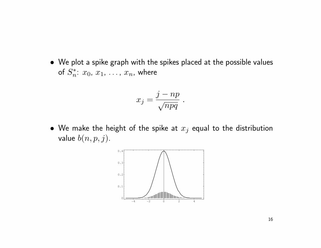
• We plot a spike graph with the spikes placed at the possible valuesof S∗n: x0, x1, . . . , xn, where

xj =j − np√

npq.

• We make the height of the spike at xj equal to the distributionvalue b(n, p, j).

16

• We plot a spike graph with the spikes placed at the possible valuesof S∗n: x0, x1, . . . , xn, where

xj =j − np√

npq.

• We make the height of the spike at xj equal to the distributionvalue b(n, p, j).

-4 -2 0 2 40

0.1

0.2

0.3

0.4

16

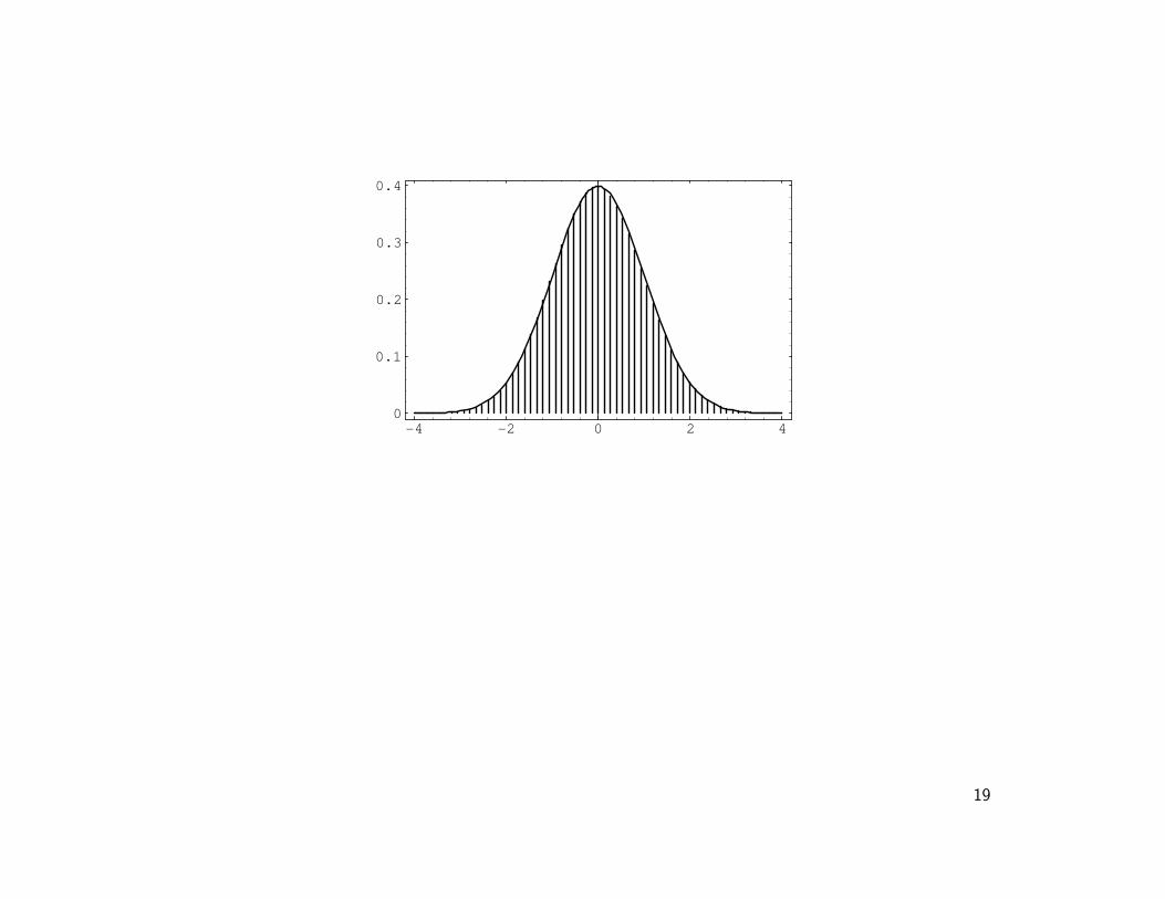
• Let ε be the distance between consecutive spikes.

• to change the spike graph so that the area under this curve hasvalue 1, we need only multiply the heights of the spikes by 1/ε.

• We see that

ε =1√npq

.

17

• Let us fix a value x on the x-axis and let n be a fixed positiveinteger.

• Then the point xj that is closest to x has a subscript j given bythe formula

j = 〈np + x√

npq〉 .

• Thus the height of the spike above xj will be

√npq b(n, p, j) =

√npq b(n, p, 〈np + xj

√npq〉) .

18

-4 -2 0 2 40

0.1

0.2

0.3

0.4

19

Central Limit Theorem for BinomialDistributions

Theorem. For the binomial distribution b(n, p, j) we have

limn→∞

√npq b(n, p, 〈np + x

√npq〉) = φ(x) ,

where φ(x) is the standard normal density.

20

Approximating Binomial Distributions

• To find an approximation for b(n, p, j), we set

j = np + x√

npq

• Solve for x

x =j − np√

npq.

b(n, p, j) ≈ φ(x)√npq

=1√npq

φ

(j − np√

npq

).

21

Example

• Let us estimate the probability of exactly 55 heads in 100 tossesof a coin.

• For this case np = 100 · 1/2 = 50 and√

npq =√100 · 1/2 · 1/2 = 5.

• Thus x55 = (55− 50)/5 = 1 and

P (S100 = 55) ∼ φ(1)5

=15

(1√2π

e−1/2

)

= .0484 .

22