Institute for Empirical Research in Economics University of Zurich

Working Paper Series

ISSN 1424-0459

Working Paper No. 480

Central Limit Theorems When Data Are Dependent:

Addressing the Pedagogical Gaps

Timothy Falcon Crack and Olivier Ledoit

February 2010

Central Limit Theorems When Data Are Dependent: Addressing the Pedagogical Gaps

Timothy Falcon Crack1 University of Otago

Olivier Ledoit2

University of Zurich

Version: August 18, 2009

1Corresponding author, Professor of Finance, University of Otago, Department of Finance and Quantitative Analysis, PO Box 56, Dunedin, New Zealand, tcrack@otago.ac.nz 2Research Associate, Institute for Empirical Research in Economics, University of Zurich, oledoit@iew.uzh.ch

1

Central Limit Theorems When Data Are Dependent: Addressing the Pedagogical Gaps

ABSTRACT

Although dependence in financial data is pervasive, standard doctoral-level econometrics

texts do not make clear that the common central limit theorems (CLTs) contained therein fail

when applied to dependent data. More advanced books that are clear in their CLT assumptions

do not contain any worked examples of CLTs that apply to dependent data. We address these

pedagogical gaps by discussing dependence in financial data and dependence assumptions in

CLTs and by giving a worked example of the application of a CLT for dependent data to the case

of the derivation of the asymptotic distribution of the sample variance of a Gaussian AR(1). We

also provide code and the results for a Monte-Carlo simulation used to check the results of the

derivation.

INTRODUCTION

Financial data exhibit dependence. This dependence invalidates the assumptions of

common central limit theorems (CLTs). Although dependence in financial data has been a high-

profile research area for over 70 years, standard doctoral-level econometrics texts are not always

clear about the dependence assumptions needed for common CLTs. More advanced

econometrics books are clear about these assumptions but fail to include worked examples of

CLTs that can be applied to dependent data. Our anecdotal observation is that these pedagogical

gaps mean that doctoral students in finance and economics choose the wrong CLT when data are

dependent.

2

In what follows, we address these gaps by discussing dependence in financial data and

dependence assumptions in CLTs, giving a worked example of the application of a CLT for

dependent data to the case of the derivation of the asymptotic distribution of the sample variance

of a Gaussian AR(1), and presenting a Monte-Carlo simulation used to check the results of the

derivation. Details of the derivations appear in Appendix A, and MATLAB code for the Monte-

Carlo simulation appears in Appendix B.

DEPENDENCE IN FINANCIAL DATA

There are at least three well-known explanations for why dependence remains in financial

data, even though the profit-seeking motives of thousands of analysts and traders might naively

be expected to drive dependence out of the data: microstructure effects, rational price formation

that allows for dependence, and behavioral biases. First, microstructure explanations for

dependence include robust findings such as thin trading induced index autocorrelation [Fisher,

1966, p. 198; Campbell, Lo, and MacKinlay, 1997, p. 84], spurious cross-autocorrelations

[Campbell, Lo, and MacKinlay, 1997, p. 129], genuine cross-autocorrelations [Chordia and

Swaminathan, 2000], and bid-ask bounce induced autocorrelation [Roll, 1984; Anderson et al.,

2006]. Second, we may deduce from Lucas [1978], LeRoy [1973], and Lo and MacKinlay

[1988] that, even if stock market prices satisfy the “efficient markets hypothesis,” rational prices

need not follow random walks. For example, some residual predictability will remain in returns

if investor risk aversion is high enough that strategies to exploit this predictability are considered

by investors to be too risky to undertake. Third, behavioral biases like “exaggeration,

oversimplification, or neglect” as identified by Graham and Dodd [1934, p. 585] are robust

sources of predictability. Popular examples of these include DeBondt and Thaler [1985, 1987],

3

who attribute medium-term reversal to investor over-reaction to news, and Jegadeesh and Titman

[1993], who attribute short-term price momentum to investor under-reaction to news. More

recently, Frazzini [2006] documents return predictability driven by the “disposition effect” (i.e.,

investors holding losing positions, selling winning positions, and therefore under-reacting to

news).

Dependence in financial data causes problems for statistical tests. Time series correlation

“…is known to pollute financial data…and to alter, often severely, the size and power of testing

procedures when neglected” [Scaillet and Topaloglou, 2005, p. 1]. For example, Hong et al.

[2007] acknowledge the impact of time series dependence in the form of both volatility

clustering and weak autocorrelation for stock portfolio returns. They use a CLT for dependent

data from White [1984] to derive a test statistic for asymmetry in the correlation between

portfolio and market returns depending upon market direction. Cross-sectional correlation also

distorts test statistics and the use of CLTs. For example, Bollerslev et al. [2007] discuss cross-

correlation in stock returns as their reason for abandoning CLTs altogether when trying to derive

an asymptotic test statistic to detect whether intradaily jumps in an index are caused by co-jumps

in individual index constituents. Instead they choose a bootstrapping technique. They argue that

the form of the dependence is unlikely to satisfy the conditions of any CLT, even one for

dependent data. Other authors assume independence in order to get a CLT they can use. For

example, Carrera and Restout [2008, p. 8], who admit their “assumption of independence across

individuals is quite strong but essential in order to apply the Lindberg-Levy central limit theorem

that permits [us] to derive limiting distributions of tests.”

Barbieri et al. [2008] discuss the importance of dependence in financial data. They

discuss CLTs and use their discussion to motivate discussion of general test statistics that are

4

robust to dependence and other violations of common CLTs (e.g., infinite variance and non-

stationarity). Barbieri et al. [2009] discuss CLTs in finance and deviations from the assumptions

of standard CLTs (e.g., time series dependence and time-varying variance). They even go so far

as to suggest that inappropriate use of CLTs that are not robust to violations of assumptions may

have led to risk-management practices (e.g., use of Value at Risk [VaR]) that failed to account

for extreme tail events and indirectly led to the global recession that began in 2007.

Brockett [1983] also discusses misuse of CLTs in risk management. This is, however, an

example of the “large deviation” problem (rather than a central limit problem) discussed in Feller

[1971, pp. 548–553]. Cummins [1991] provides an excellent explanation of Brockett’s work, and

Lamm-Tennant et al. [1992] and Powers et al. [1998] both warn the reader about the problem.

Carr and Wu [2003] are unusual in that they deliberately build a model of stock returns

that violates the assumptions of a CLT. They do so because they observe patterns in option

implied volatility smiles that are inconsistent with the CLT assumptions being satisfied. The

assumption they violate is, however, finiteness of second moments rather than independence.

Research interest in dependence in financial data is nothing new. There has been a

sustained high level of research into dependence in financial data stretching, for example, from

Cowles and Jones [1937] to Fama [1965], to Lo and MacKinlay [1988], to Egan [2008], to

Bajgrowicz and Scaillet [2008], to Barbieri et al. [2008, 2009], and beyond.

Given that dependence in financial data is widespread, causes many statistical problems,

and is the topic of much research, careful pedagogy in the area of the application of CLTs to

dependent data is required.

5

PEDAGOGICAL GAPS

We have identified two pedagogical gaps in the area of the application of CLTs to

dependent data. First, standard doctoral-level econometrics texts do not always make clear the

assumptions required for common CLTs, and they may, by their very nature, fail to contain more

advanced CLTs. For example, looking at the Lindberg-Levy and Lindberg-Feller CLTs in

Greene [2008], it is not at all clear that they do not apply to dependent data [see Theorems

D.18A and D.19A in Greene, 2008, pp. 1054–1055]. Only very careful reading of earlier

material in the book, combined with considerable inference, reveals the full assumptions of these

theorems. The assumptions for these two theorems are, however, clearly stated in more advanced

books [see DasGupta, 2008, p. 63; Davidson, 1997, Theorems 23.3 and 23.6; Feller, 1968, p.

244; Feller, 1971, p. 262; and White, 1984 and 2001, Theorems 5.2 and 5.6]. Second, even

where the assumptions for the simple CLTs do appear clearly and where the more advanced

CLTs for dependent data are present, we have been unable to find any worked example showing

the application of the more advanced CLTs to concrete problems. For example, although Hong et

al. [2007] use a CLT for dependent data from White [1984], they gloss over the implementation

details because theirs is a research paper, not a pedagogical one.

These pedagogical gaps make the area of the application of advanced CLTs to cases of

dependent data poorly accessible to many doctoral students. We believe that the best way to

address this problem is by providing a worked example using a CLT for dependent data in a

simple case. So, in what follows, we derive the asymptotic distribution of the sample variance of

a Gaussian AR(1) process using a CLT from White [1984, 2001]. We also derive the asymptotic

6

distribution of the sample mean for the process. This latter derivation does not need a CLT, but

the result is needed for the asymptotic distribution of the sample variance.

WORKED EXAMPLE OF A CLT FOR DEPENDENT DATA

We assume that the random variable tX follows a Gaussian AR(1) process:

,)(= 1 ttt XX εμρμ +−+ − (1)

where )(0, 2εσε NIIDt ∼ , “IID” means independent and identically distributed, and “ ),( baN ”

denotes a Normal distribution with mean a and variance b . The only other assumption we make

in the paper is that 1|<| ρ (so that tX is stationary).

The functional form of (1) is the simplest example of a non-IID data-generating process.

By restricting our attention to an AR(1), we minimize the complexity of the dependence in the

data while still being able to demonstrate the use of a CLT for dependent data. Our asymptotic

results may be derived without our assumption of Gaussian increments [e.g., using theorems in

Fuller, 1996, Section 6.3; or Brockwell and Davis, 1991, Section 6.4]. The Gaussian

specification of the problem allows, however, for a cleaner pedagogical illustration using an

elegant CLT from White [1984, 2001]. It also allows for a cleaner specification of the Monte-

Carlo simulation we perform.

The Gaussian AR(1) process tX is stationary and ergodic by construction (see the proof

of Lemma 4 in Appendix A). Stationarity and ergodicity are strictly weaker than the IID

assumption of the classical theorems in probability theory (e.g., the Lindberg-Levy and

Lindberg-Feller CLTs). Thus, these theorems do not apply. Stationarity and ergodicity are

sufficient, however, for us to derive asymptotic results analogous to those available in the case

where tX is IID.

7

Let μ̂ , and 2σ̂ denote the usual sample mean and variance of the tX 's,

.)ˆ(1

1ˆ ,1ˆ 2

1=

2

1=μσμ −

−≡≡ ∑∑ t

n

tt

n

tX

nandX

n (2)

The following two lemmas and theorem give the asymptotic distribution of the sample mean μ̂

of the Gaussian AR(1) process.

Lemma 1 We have the following exact distributional result for a Gaussian AR(1):

.)(1

0,1

)ˆ( 2

20

⎟⎟⎠

⎞⎜⎜⎝

⎛−⎥

⎦

⎤⎢⎣

⎡ −⋅

−+−

ρσ

ρρμμ εN

nXXn n ∼ (3)

Proof:

See Appendix A.

Lemma 2 The following probability limit result holds for the second term on the left-

hand side of (3):

0.=1

0⎥⎦

⎤⎢⎣

⎡ −⋅

− nXXplim n

ρρ (4)

Proof:

See Appendix A.

Theorem 1 We have the following asymptotic distributional result for the sample mean

of a Gaussian AR(1) process:1

,1

)(10,)ˆ(2

⎟⎟⎠

⎞⎜⎜⎝

⎛−+

−ρρσμμ Nn

A∼ (5)

where 2σ is the variance of tX .

8

Proof:

Apply Lemma 2 to (3) in Lemma 1 to deduce the asymptotic Normality of )ˆ( μμ −n .

Then use the stationarity of tX (recall 1|<| ρ ) to replace 2εσ by )(1 22 ρσ − , thus completing the

proof. This proof does not require a CLT, but one is needed in the proof of Lemma 4. See van

Belle [2002, p. 8] for a related result and DasGupta [2008, p. 127] for a related exercise.

The following two lemmas and theorem give the asymptotic distribution of the sample

variance 2σ̂ of the Gaussian AR(1) process.

Lemma 3 We may rewrite the term )ˆ( 22 σσ −n as follows:

,ˆˆ1)(=)ˆ(

2222222

nnnsnsnn σσσσσ +⎟⎟

⎠

⎞⎜⎜⎝

⎛⎟⎠⎞

⎜⎝⎛ −

−−−− (6)

where .)(1 21=

2 μ−≡ ∑ tn

tX

ns

Proof:

Direct algebraic manipulation and cancellation of terms.

Lemma 4 The following asymptotic distributional and probability limit results hold for

the three terms on the right-hand side of (6):

,)(1

)(120,)( 2

2422

⎟⎟⎠

⎞⎜⎜⎝

⎛−+

−ρρσσ Nsn

A∼ (7)

andn

nsnplim 0,=ˆ1 22⎥⎦

⎤⎢⎣

⎡⎟⎟⎠

⎞⎜⎜⎝

⎛⎟⎠⎞

⎜⎝⎛ −

− σ (8)

0.=ˆ 2

⎥⎦

⎤⎢⎣

⎡n

plim σ (9)

9

Proof:

This is the most difficult derivation. It requires a CLT for dependent data. See Appendix

A.

Theorem 2 We have the following asymptotic distributional result for the sample

variance of a Gaussian AR(1) process:

.)(1

)(120,)ˆ( 2

2422

⎟⎟⎠

⎞⎜⎜⎝

⎛−+

−ρρσσσ Nn

A∼ (10)

Proof:

Apply the three results in Lemma 4 to the three right-hand side terms, respectively,

appearing in Lemma 3, and deduce the result directly.

The asymptotic results for μ̂ in (5) of Theorem 1 and for 2σ̂ in (10) of Theorem 2 have

elegant interpretations. The higher is the degree of positive autocorrelation ρ , the larger is the

standard error of both μ̂ and 2σ̂ —higher positive ρ means fewer effectively independent

observations of tX . Similarly, the higher is the degree of negative autocorrelation, then the

larger is the standard error of 2σ̂ . We leave the reader with a small challenge: Deduce the

qualitative explanation for why larger negative autocorrelation reduces the standard error of μ̂ .

MONTE-CARLO SIMULATION

We have found that a Monte-Carlo simulation of the process and of the asymptotic

distributions of the sample estimators aids doctoral student understanding significantly. We

10

therefore present MATLAB code for a Monte-Carlo simulation, and we plot the resulting

theoretical and simulated empirical asymptotic distributions.

In the case of the Gaussian AR(1), doctoral students who incorrectly use CLTs for

independent data invariably conclude that the variance on the left-hand side of (10) is 42σ rather

than )(1

)(122

24

ρρσ

−+ . You may then ask your students to perform a Monte-Carlo simulation of the

Gaussian AR(1) process with 0≠ρ , so that they can demonstrate for themselves that they have

statistically significantly underestimated the true standard error.

A portion of our MATLAB code for the Monte-Carlo simulation appears in Appendix B.

We choose the values 0=μ , 0.90=ρ , and 0.50=εσ . Figures 1 and 2 compare the realized

empirical distribution to the theoretical results for both the asymptotic distribution of 2σ̂ and the

actual large sample distribution of 2σ̂ (they are scaled versions of each other because we use the

same random seed). We do not show the analogous results for μ̂ .

Two pedagogical purposes are served by the Monte-Carlo simulation. First, our

experience is that when a doctoral student simulates the process, repeatedly collects the

asymptotic sample statistics, and then forms a distribution, he or she only then attains a clear

concrete notion of what an asymptotic distribution actually is. Second, by comparing the realized

asymptotic distribution to the derived theoretical one, the students understand the power of a

Monte-Carlo in attempting to confirm or deny the consistency of a difficult analytical result—

each of Figures 1 and 2 clearly distinguishes between the competing asymptotic distributions.

[Insert Figures 1 and 2 about here]

11

CONCLUSIONS

In our experience, finance and economics doctoral students have limited exposure to the

use of central limit theorems for dependent data. Given that dependence in financial data is

widespread, causes many statistical problems, and is the topic of much research, careful

pedagogy in the area of the application of CLTs to dependent data is required. We identify,

however, two pedagogical gaps in the area. We fill these gaps by discussing dependence in

financial data and dependence assumptions for CLTs and by showing how to use a CLT for

dependent data to derive the asymptotic distribution of the sample estimator of the variance of a

Gaussian AR(1) process. We also present a Monte-Carlo simulation to aid student understanding

of asymptotic distributions and to illustrate the use of a Monte-Carlo in attempting to confirm or

deny an analytical result.

ENDNOTES

1. If a sequence nb of random variables converges in distribution to a random variable Z

(often written “ Zbd

n → ”), then nb is said to be asymptotically distributed as ZF , where ZF is the

distribution of Z . This is denoted here by “ Z

A

n Fb ∼ ” [as in White, 2001, p. 66].

2. Note that White's “stationarity” is strict stationarity. That is, ∞1=}{ ttZ and ∞

− 1=}{ tktZ have

the same joint distribution for every 0>k [see White, 2001, p. 43; and Davidson 1997, p. 193].

12

REFERENCES

Anderson, R. M., K. S. Eom, S. B. Hahn, and J. H. Park. “Stock Return Autocorrelation Is Not

Spurious,” Working Paper, UC Berkeley and Sunchon National University, (May 2008).

Bajgrowicz, P. and O. Scaillet. “Technical Trading Revisited: Persistence Tests, Transaction

Costs, and False Discoveries,” Swiss Finance Institute Research Paper No. 08-05, (January 1,

2008). Paper available at SSRN: http://ssrn.com/abstract=1095202.

Barbieri, A., V. Dubikovsky, A. Gladkevich, L. R. Goldberg, and M. Y. Hayes. “Evaluating Risk

Forecasts with Central Limits,” (July 9, 2008). Available at SSRN:

http://ssrn.com/abstract=1114216.

Barbieri, A., V. Dubikovsky, A. Gladkevich, L. R. Goldberg, and M. Y. Hayes. “Central Limits

and Financial Risk,” (March 11, 2009). MSCI Barra Research Paper No. 2009-13. Available at

SSRN: http://ssrn.com/abstract=1404089.

Bollerslev, T., T.H. Law, and G. Tauchen, “Risk, Jumps, and Diversification,” (August 16,

2007). CREATES Research Paper 2007-19. Available at SSRN:

http://ssrn.com/abstract=1150071.

Brockett, P. L. “On the Misuse of the Central Limit Theorem in Some Risk Calculations,”

The Journal of Risk and Insurance 50(4) (1983), 727–731.

13

Brockwell, P. J. and R. A. Davis. Time Series: Theory and Methods (New York, 1991), 2nd

Edition, Springer.

Campbell, J. Y., A. W. Lo, and A. C. MacKinlay. The Econometrics of Financial Markets,

(Princeton, 1997), Princeton University Press.

Carr, P. and Liuren Wu, “The Finite Moment Log Stable Process and Option Pricing,”

Journal of Finance 58(2) (2003), 753–777.

Carrera, J. E. and R. Restout. “Long Run Determinants of Real Exchange Rates in Latin

America” (April 1, 2008). GATE Working Paper No. 08-11. Available at SSRN:

http://ssrn.com/abstract=1127121.

Chordia, T. and B. Swaminathan, “Trading Volume and Cross-Autocorrelations in Stock

Returns,” Journal of Finance 55(2) (2000), 913–935.

Cowles, A. and H. Jones. “Some A Posteriori Probabilities in Stock Market Action,”

Econometrica 5 (1937), 280–294.

Cummins, J. D. “Statistical and Financial Models of Insurance Pricing and the Insurance Firm,”

The Journal of Risk and Insurance 58(2) (June, 1991), 261–302.

DasGupta, A. Asymptotic Theory of Statistics and Probability, (New York, 2008), Springer.

14

Davidson, J. Stochastic Limit Theory (New York, 1997), Oxford University Press.

DeBondt, W. and R. Thaler. “Does the Stock Market Overreact?” Journal of Finance 40 (1985),

793–805.

DeBondt, W. and R. Thaler. “Further Evidence on Investor Overreaction and Stock Market

Seasonality,” Journal of Finance 42 (1987), 557–582.

Egan, W. J. “Six Decades of Significant Autocorrelation in the U.S. Stock Market” (January 20,

2008). Available at SSRN: http://ssrn.com/abstract=1088861.

Fama, E. F. “The Behavior of Stock Market Prices,” Journal of Business 38 (1965), 34–105.

Feller, W. An Introduction to Probability Theory and Its Applications (New York, 1968),

Volume I, 3rd Edition, John Wiley and Sons.

Feller, W. An Introduction to Probability Theory and Its Applications (New York, 1971),

Volume II, 2nd Edition, John Wiley and Sons.

Fisher, L., “Some New Stock Market Indexes,” Journal of Business 39 (1966), 191–225.

15

Fuller, W. A. Introduction to Statistical Time Series (New York, 1996), 2nd Edition, John Wiley

and Sons.

Frazzini, A., “The Disposition Effect and Underreaction to News,” Journal of Finance 61(4),

2017–2046.

Graham, B. and D. Dodd, Security Analysis: The Classic 1934 Edition, (New York, 1934),

McGraw-Hill.

Greene, W. H. Econometric Analysis (Upper Saddle River, 2008), 6th Edition, Prentice Hall.

Hamilton, J. D. Time Series Analysis (Princeton, 1994), Princeton University Press.

Hong, Y., J. Tu, and G. Zhou. “Asymmetries in Stock Returns: Statistical Tests and Economic

Evaluation,” Review of Financial Studies 20(5) (2007), 1547–1581.

Ibragimov, I. A. and Y. V. Linnik Independent and Stationary Sequences of Random Variables

(The Netherlands, 1971), ed. by J. F. C. Kingman, Wolters-Noordhoff Publishing Groningen.

Jegadeesh, N. and S. Titman. “Returns to Buying Winners and Selling Losers: Implications for

Stock Market Efficiency,” Journal of Finance 48 (1993), 65–91.

16

Lamm-Tennant, J., L. T. Starks, and L. Stokes. “An Empirical Bayes Approach to Estimating

Loss Ratios,” Journal of Risk and Insurance 59(3) (1992), 426–442.

LeRoy, S. F. “Risk Aversion and the Martingale Property of Stock Prices,” International

Economic Review 14(2) (1973), pp. 436–446

Lo, A. W. and A. C. MacKinlay. “Stock Market Prices Do Not Follow Random Walks: Evidence

from a Simple Specification Test,” Review of Financial Studies 1(1) (1988), 41–66.

Lucas, R. E., “Asset Prices in an Exchange Economy,” Econometrica 46(6) (1978), 1429–1445.

Powers, M.R., M. Shubik, and S.T. Yao, “Insurance Market Games: Scale Effects and Public

Policy,” Journal of Econometrics 67(2) (1998), 109–134.

Roll, R. “A Simple Implicit Measure of the Effective Bid Ask Spread in an Efficient Market,”

Journal of Finance 39(4) (1984), 1127–1139.

Rosenblatt, M. “Dependence and Asymptotic Dependence for Random Processes,” Studies in

Probability Theory (Washington, D.C., 1978), Murray Rosenblatt (ed.), Mathematical

Association of America, 24–45.

Scaillet, O. and N. Topaloglou, “Testing for Stochastic Dominance Efficiency” (July 2005).

FAME Research Paper No. 154. Available at SSRN: http://ssrn.com/abstract=799788.

17

van Belle, Gerald, Statistical Rules of Thumb (New York, 2002), Wiley Series in Probability and

Statistics.

White, H. Asymptotic Theory for Econometricians (San Diego, 1984), Academic Press.

White, H. Asymptotic Theory for Econometricians (San Diego, 2001), Revised 2nd Edition,

Academic Press.

18

APPENDIX A. DERIVATIONS

Proof of Lemma 1: Rewrite the left-hand side of (3) in terms of the residual tε (the

exact distribution of which is known).

⎥⎦

⎤⎢⎣

⎡ −⋅

−+−

nXXn n 0

1)ˆ(

ρρμμ

⎥⎦

⎤⎢⎣

⎡⎟⎠⎞

⎜⎝⎛ −

+−−− n

XXn n 0)ˆ)((1)(1

= ρμμρρ

⎥⎦

⎤⎢⎣

⎡⎥⎦

⎤⎢⎣

⎡⎟⎠⎞

⎜⎝⎛ −

−−−−− n

XXn n 0)ˆ()ˆ()(1

= μμρμμρ

⎥⎦

⎤⎢⎣

⎡⎥⎦

⎤⎢⎣

⎡⎟⎠⎞

⎜⎝⎛ −

−−−−− ∑∑ n

XXXn

Xn

n nt

n

tt

n

t

0

1=1=)(1)(1

)(1= μρμ

ρ

⎥⎦

⎤⎢⎣

⎡⎥⎦

⎤⎢⎣

⎡−−−−−

−∑∑ )()()(

)(11= 0

1=1=XXXX

n nt

n

tt

n

tμρμ

ρ

⎥⎦

⎤⎢⎣

⎡−−−

− −∑∑ )()()(1

1= 11=1=

μρμρ t

n

tt

n

tXX

n

[ ])()()(1

1= 11=

μρμρ

−−−− −∑ tt

n

t

XXn

,)(1

1=1=

t

n

tnε

ρ ∑−

where the last line uses the definition of tε implicit within (1). We may now use

)(0, 2εσε NIIDt ∼ to deduce

,)(1

0,)(1

12

2

1=⎟⎟⎠

⎞⎜⎜⎝

⎛−− ∑ ρσε

ρεN

n t

n

t∼

thus proving the lemma.

19

Proof of Lemma 2:

Let “ ),(⋅var ” “ ),,( ⋅⋅cov ” and “ ),,( ⋅⋅corr ” denote the unconditional variance, covariance,

and correlation operators, respectively. Let 2σ denote )( tXvar . The term

]))/[(1( 0 nXX n ρρ −− is shown to have variance of order )(1/nO as follows:

)(1

1=)(1 0

20 XXvar

nnXXvar n

n −⎟⎟⎠

⎞⎜⎜⎝

⎛−⎥

⎦

⎤⎢⎣

⎡ −⋅

− ρρ

ρρ

[ ]),(2)()(1

1= 00

2

XXcovXvarXvarn nn −+⎟⎟

⎠

⎞⎜⎜⎝

⎛− ρρ

[ ]σσσσρ

ρ ),(21

1= 022

2

XXcorrn n−+⎟⎟

⎠

⎞⎜⎜⎝

⎛−

.1

422

⎟⎟⎠

⎞⎜⎜⎝

⎛−

≤ρ

ρσn

(11)

This derivation assumes 1|<| ρ (so that stationarity of tX gives 20 =)(=)( σXvarXvar n ). We

also use 1),( 0 −≥XXcorr n at the last step.

Tchebychev's Inequality [Greene 2008, p. 1040] says that for random variable V and

small 0,>δ

.)()|>)((| 2δδ VvarVEVP ≤−

We may apply Tchebychev's Inequality to ]))/[(1( 0 nXXV nn ρρ −−≡ , and use (11) to find

20 )(>)(

1 δδ

ρρ nn Vvar

nXXP ≤⎟⎟

⎠

⎞⎜⎜⎝

⎛ −⋅

−

.1

42

2

2

⎟⎟⎠

⎞⎜⎜⎝

⎛−

≤ρ

ρδσ

n

20

Thus, for any 0>δ , we have 0=)|>(|lim δnn VP∞→ . That is, 0=nVplim , thus proving the

lemma.

Proof of Lemma 4: We demonstrate each of Equations (7), (8), and (9) in turn. We begin

with the proof of the asymptotic result in (7):

,)(1

)(120,)( 2

2422

⎟⎟⎠

⎞⎜⎜⎝

⎛−+

−ρρσσ Nsn

A∼

where 21=

2 )(1 μ−≡ ∑ tn

tX

ns , and )(=2

tXvarσ . To derive this result, we apply the following

CLT for non-IID data adapted directly from White [1984].

Theorem [from White 1984, Theorem 5.15, p. 118]

Let tℑ be the sigma-algebra generated by the entire current and past history of a

stochastic variable tZ ; let jt ,ℜ be the revision made in forecasting tZ when information

becomes available at time jt − , that is, )|()|( 1, −−− ℑ−ℑ≡ℜ jttjttjt ZEZE ; let nZ denote the

sample mean of nZZ ,,1 … ; and let )(2nn Znvar≡σ . Then, if the sequence }{ tZ satisfies the

following conditions: 1. }{ tZ is stationary;2 2. }{ tZ is ergodic; 3. ∞<)( 2tZE ; 4.

0)|(..

0

mq

mZE →ℑ− as ∞→m ; and 5. ( )[ ] ∞ℜ∑∞ <1/20,0= jj

var , we obtain the results 22 σσ →n , as

∞→n , and if 0>2σ , then (0,1)NZn An ∼

σ.

We apply the theorem to .)( 22 σμ −−≡ tt XZ With this definition of tZ , we obtain

,=)(1/= 221=

σ−∑ sZnZ tn

tn and, thus, ).(= 22 σ−snZn n However, before we can apply the

21

theorem, we must check that its five conditions are satisfied, and we must calculate

)(lim=lim 2nnnn Znvar∞→∞→ σ . We begin by checking the five conditions.

Condition 1: We have assumed 1|<| ρ . Thus, our Gaussian AR(1) process tX is stationary.

Stationarity of tX yields stationarity of tZ immediately (by definition of tZ ).

Condition 2: White [2001, p. 48] uses Ibragimov and Linnik [1971, pp. 312–313] to deduce that

a Gaussian AR(1) with 1|<| ρ is strong mixing. White [2001, p. 48] then uses Rosenblatt [1978]

to state that strong mixing plus stationarity (recall 1|<| ρ ) implies ergodicity. It follows that tX

is ergodic. This yields ergodicity of tZ immediately (by definition of tZ ).

Condition 3: We note first that since tε is Gaussian, then so too is tX [Hamilton 1994, p. 118].

It is well known that if ),( 2σμNX t ∼ , then 44 3=])[( σμ−tXE . It follows that

]))[((=)( 2222 σμ −−tt XEZE

])(2)[(= 4224 σμσμ +−−− tt XXE

.<2=23= 4444 ∞+− σσσσ (12)

Condition 4: To show that 0)|(..

0

mq

mZE →ℑ− as ∞→m , we must show that 0)|(..mq

mttZE →ℑ − as

∞→m in the special case 0=t . In fact, we can prove convergence in quadratic mean for any t

if we can show 0))]|(([ 2 →ℑ −mttZEE as ∞→m [see White, 1984, p. 117]. To

derive )|( mttZE −ℑ , we first consider the term 22 )(= μσ −+ tt XZ as follows:

22

ttt XX εμρμ +−− − )(= 1

.)(=1

0=kt

km

kmt

m X −

−

− ∑+− ερμρ (13)

With 22 )(= μσ −+ tt XZ , it follows from (13) that

⎥⎥⎦

⎤

⎢⎢⎣

⎡ℑ⎟

⎠

⎞⎜⎝

⎛+−ℑ+ −−

−

−− ∑ mtktk

m

kmt

mmtt XEZE

21

0=

2 )(=)|( ερμρσ

221

0=

22 0)(= εσρμρ km

kmt

m X ∑−

− ++−

22

222

11)(= εσρ

ρμρ ⎟⎟⎠

⎞⎜⎜⎝

⎛−−

+−−

m

mtm X

)](1[11)(= 22

2

222 ρσ

ρρμρ −⎟⎟

⎠

⎞⎜⎜⎝

⎛−−

+−−

m

mtm X

).(1)(= 2222 mmt

m X ρσμρ −+−− (14)

If we now cancel 2σ from both sides of (14), we find

.=])[(=)|( 2222mt

mmt

mmtt ZXZE −−− −−ℑ ρσμρ (15)

It follows that 4424222 2=)(=)]([=))]|(([ σρρρ mmt

mmt

mmtt ZEZEZEE −−−ℑ (using (12) and

stationarity of tZ ). With 1|<| ρ , we deduce that 0))]|(([ 2 →ℑ −mttZEE as ∞→m , and, thus, that

0)|(..mq

mttZE →ℑ − as ∞→m [using White, 1984, p. 117], as required.

Condition 5: Applying (15) to the definition of jt ,ℜ yields

)|()|( 1, −−− ℑ−ℑ≡ℜ jttjttjt ZEZE

23

.= 1)(1)2(2

+−+

− − jtj

jtj ZZ ρρ (16)

By definition, 0,=)( tZE so 0=)( , jtE ℜ , and, thus, )(=)( 2,, jtjt Evar ℜℜ . Manipulating (16), we

get

)(=)( 2,, jtjt Evar ℜℜ

)]([= 21)(

1)2(2+−

+− − jt

jjt

j ZZE ρρ

( ) ),(22= 1)(2441)4(4

+−−++ −+ jtjt

jjj ZZEρσρρ

( ) ),(22= 12441)4(4

−++ −+ tt

jjj ZZEρσρρ (17)

where we used (12) and the fact that 0=)(=)( 1)( +−− jtjt ZEZE . We also used stationarity of tZ to

rewrite )( 1)( +−− jtjt ZZE as )( 1−tt ZZE .

The term )( 1−tt ZZE in (17) may be expanded as follows:

)]))(()[((=)( 221

221 σμσμ −−−− −− tttt XXEZZE

.])()[(= 421

2 σμμ −−− −tt XXE

Plugging this expression for )( 1−tt ZZE into (17) gives

( ) 41)4(4, 2=)( σρρ ++ℜ jj

jtvar

( )421

224 ])()[(2 σμμρ −−−− −+

ttj XXE

( ) ( ),)(22= 421

22441)4(4 σρσρρ −−+ −++

ttjjj YYE (18)

where )( μ−≡ tt XY . The term )( 21

2−tt YYE is a special case of a more general term )( 22

dtt YYE − ,

which we now evaluate (we need the general term later in the proof). From the definition of the

Gaussian AR(1) (1) and from (13), we deduce that ktkd

kdtd

t YY −−

− ∑+ ερρ 1

0== and that tY is

Gaussian with zero-mean. It follows that

24

⎥⎥⎦

⎤

⎢⎢⎣

⎡⎟⎠

⎞⎜⎝

⎛+ −−

−

−− ∑ 221

0=

22 =)( dtktk

d

kdt

ddtt YYEYYE ερρ

)(2)(= 321

0=

42dtkt

kd

k

ddt

d YEEYE −−

−

− ⎟⎠

⎞⎜⎝

⎛+ ∑ ερρρ

)( 221

0=dtkt

kd

kYEE −−

−

⎥⎥⎦

⎤

⎢⎢⎣

⎡⎟⎠

⎞⎜⎝

⎛+ ∑ ερ

221

0=

242 03= εσρσσρ kd

k

d ∑−

++

)](1[113= 22

2

2242 ρσ

ρρσσρ −⎟⎟

⎠

⎞⎜⎜⎝

⎛−−

+d

d

),2(1= 24 dρσ + (19)

where we used independence of dtY − and kt−ε for dk < to separate expectations in the cross-

product term. We also used the mean-zero Normality of dtY − to write 0=)( 3dtYE − , and

44 3=)( σdtYE − . If we now set 1=d in (19) and plug this into (18), we obtain

( ) ( )4242441)4(4, )2(122=)( σρσρσρρ −+−+ℜ ++ jjj

jtvar

.)(12= 444 jρρσ − (20)

Thus, .)(12=)(=)]([ 2442,

1/2,

jjtjt Evar ρρσ −ℜℜ It follows that

( )( ) j

jjt

jvar 2

0=

441/2,

0=)(12= ρρσ ∑∑

∞∞

−ℜ

2

44

1)(12

=ρ

ρσ−

−

2

224

1))(1(12

=ρ

ρρσ−

−+

25

. < 1

)(12= 2

24

∞−+ρρσ

This latter result holds in the special case 0=t , so the fifth and final prerequisite for applying

White's Theorem to tZ is satisfied.

We must now find )(lim=lim 22nnnn Znvar∞→∞→≡ σσ . Recall that we have

22)(= σμ −−tt XZ , so that )(= 22 σ−snZn n , where 21=

21=

2 )(1/=)()(1/ tn

ttn

tYnXns ∑∑ −≡ μ .

With 2σ a constant, we know that )(=)( 2snvarZnvar n . It is easier to work with )( 2nsvar , so

we do that and then adjust the result.

⎟⎠

⎞⎜⎝

⎛∑ 2

1=

2 =)( t

n

tYvarnsvar

2

2

1=

22

1== ⎥

⎦

⎤⎢⎣

⎡⎟⎠

⎞⎜⎝

⎛−

⎥⎥⎦

⎤

⎢⎢⎣

⎡⎟⎠

⎞⎜⎝

⎛ ∑∑ t

n

tt

n

tYEYE

2222

1=1=)(= σnYYE st

n

s

n

t−⎥

⎦

⎤⎢⎣

⎡ ∑∑

( ) 224221

1=2=)()(2= σnYnEYYE tdtt

t

d

n

t−⎥

⎦

⎤⎢⎣

⎡+−

−

∑∑

( ) ,)(3212= 22421

1=2=

4 σσρσ nndt

d

n

t−⎥

⎦

⎤⎢⎣

⎡++∑∑

−

(21)

where we used (19) to replace ( )22dtt YYE − . If we divide (21) by 4σ and combine the final two

terms, we get

( ) )(3212=)( 21

1=2=4

2

nnnsvar dt

d

n

t−++∑∑

−

ρσ

)(31

121)(2= 2

1)2(2

2=nnt

tn

t−+⎥

⎦

⎤⎢⎣

⎡⎟⎟⎠

⎞⎜⎜⎝

⎛−

−+−

−

∑ ρρρ

26

It is easily shown that nnntn

t2)(3=1)(2

2=+−−−∑ , so we get some cancellation as follows:

nnnsvar tn

t21)(

14=)( 1)2(

2=2

2

4

2

+⎥⎦

⎤⎢⎣

⎡−−

−−∑ρ

ρρ

σ

⎟⎟⎠

⎞⎜⎜⎝

⎛−

−⋅

−−

−−+− −

2

1)2(2

2

2

2

22

11

14

1)(121)(4=

ρρρ

ρρ

ρρρ nnn

⎥⎦

⎤⎢⎣

⎡⎟⎟⎠

⎞⎜⎜⎝

⎛−

−+

−−

−−+ −

2

1)2(2

2

2

2

22

111

14

1224=

ρρρ

ρρ

ρρρ nnnn

.)(1

)(14)(1

)(12= 22

22

2

2

ρρρ

ρρ

−−

−−+ nn (22)

It follows immediately that )(1

)(12)( 2

242

ρρσ

−+

→snvar as ∞→n . Using this result in the last

part of White's theorem yields

,)(1

)(120,)( 2

2422

⎟⎟⎠

⎞⎜⎜⎝

⎛−+

−ρρσσ Nsn

A∼

thus proving (7)—the first of the three parts of Lemma 4.

To demonstrate (8)—the second of the three parts of Lemma 4—we need the probability

limit of ( )( )22 ˆ1)/( σnnsn −− . Direct algebraic manipulation yields

222 )ˆ(=ˆ1 μμσ −⎥⎦

⎤⎢⎣

⎡⎟⎟⎠

⎞⎜⎜⎝

⎛⎟⎠⎞

⎜⎝⎛ −

− nn

nsn

2

2

2

1)(1)ˆ(

1)(11=

⎥⎥⎥⎥⎥

⎦

⎤

⎢⎢⎢⎢⎢

⎣

⎡

−+

−⋅⎥⎦

⎤⎢⎣

⎡−+

ρρσμμ

ρρσ n

n

,1

)(11= 22

nQn ⎥

⎦

⎤⎢⎣

⎡−+ρρσ (23)

27

where

⎥⎥⎥⎥⎥

⎦

⎤

⎢⎢⎢⎢⎢

⎣

⎡

−+

−≡

ρρσμμ

1)(1)ˆ(

2

nQn is asymptotically standard Normal (a consequence of Theorem 1). We

may now apply a result analogous to Slutsky's Theorem for probability limits [see Greene, 2008,

p. 1045] to deduce that 21

2 χA

nQ ∼ (that is, 2nQ is asymptotically chi-square with one degree of

freedom). Thus, 2nQ is of bounded variance. It follows that one application of Tchebychev's

Inequality to (23) produces the result:

0,=ˆ1 22⎥⎦

⎤⎢⎣

⎡⎟⎟⎠

⎞⎜⎜⎝

⎛⎟⎠⎞

⎜⎝⎛ −

− σn

nsnplim

thus proving (8)—the second of the three parts of Lemma 4.

To demonstrate (9)—the third and final part of Lemma 4—we need the probability limit

of )./ˆ( 2 nσ Algebraic manipulation gives

.)ˆ(11

=ˆ 222 μμσ −⎟⎠⎞

⎜⎝⎛

−−⎟

⎠⎞

⎜⎝⎛

− nns

nn (24)

The variance of 2s goes to zero as ∞→n (a consequence of (22)). The variance of 2)ˆ( μμ −

goes to zero as ∞→n (a consequence of 21

2 χA

nQ ∼ , from above). In (24), the coefficients

11)/( →−nn as ∞→n . It follows that 0)ˆ( 2 →σvar with n . An application of Tchebychev's

Inequality yields immediately

0,=ˆ 2

⎥⎦

⎤⎢⎣

⎡

nplim σ

thus proving the third and final part of Lemma 4.

28

APPENDIX B. MATLAB MONTE-CARLO CODE

clear;

rho=0.90;sigmae=0.50;mu=0;sigma=sigmae/sqrt(1-rho^2);

N=500000;NUMBREPS=10000; rseed=20081103; randn('seed',rseed);

collect=[ ];

for J=1:NUMBREPS

Y=[]; epsilon=randn(N,1); xpf=epsilon*sigmae;

bpf=1; apf=[1 -rho]; Y=filter(bpf,apf,xpf);

collect=[collect' [mean(Y) var(Y)]']';

end

asymeanv=0; asyvarv=2*(sigma^4)*(1+rho^2)/(1-rho^2);

asymeanv1=0; asyvarv1=2*(sigma^4); v=sqrt(N)*(collect(:,2)-sigma^2);

hpdf=[];mynormpdf=[];[M,X]=hist(v,250);M=M';X=X';dx=min(diff(X));

hpdf=M/(sum(M)*dx);

mynormpdf=(1/(sqrt(2*pi)*sqrt(asyvarv))).*exp(

-0.5*((X-asymeanv)/sqrt(asyvarv)).^ 2);

mynormpdf1=(1/(sqrt(2*pi)*sqrt(asyvarv1))).*exp(

-0.5*((X-asymeanv1)/sqrt(asyvarv1)).^2);

plot(X,[hpdf mynormpdf mynormpdf1],'k')

xlabel('Asymptotic Sample Variance of the Gaussian AR(1)');

ylabel('Frequency');

29

Figure 1. Histogram of Simulated Empirical PDF of )ˆ( 22 σσ −n

We use MATLAB to simulate a time series of 500,000 observations of the Gaussian

AR(1) using 0.90=ρ , 0.50=εσ , and 0=μ . We then record the sample variance 2σ̂ of the

process. We repeat this 10,000 times and plot (the uneven line) the realized density

of )ˆ( 22 σσ −n . We overlay on the plot the correct theoretical density ⎟⎟⎠

⎞⎜⎜⎝

⎛−+

)(1)(120, 2

24

ρρσN and

the most common incorrect student-derived theoretical density ( )40,2σN . The correct density is

the one close to the empirical density; the incorrect density is more peaked.

30

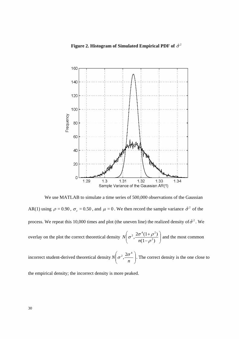
Figure 2. Histogram of Simulated Empirical PDF of 2σ̂

We use MATLAB to simulate a time series of 500,000 observations of the Gaussian

AR(1) using 0.90=ρ , 0.50=εσ , and 0=μ . We then record the sample variance 2σ̂ of the

process. We repeat this 10,000 times and plot (the uneven line) the realized density of 2σ̂ . We

overlay on the plot the correct theoretical density ⎟⎟⎠

⎞⎜⎜⎝

⎛−+

)(1)(12, 2

242

ρρσσ

nN and the most common

incorrect student-derived theoretical density ⎟⎟⎠

⎞⎜⎜⎝

⎛n

N4

2 2, σσ . The correct density is the one close to

the empirical density; the incorrect density is more peaked.