central tendency, dispersion, correlation and regression analysis

Business Statistic

Central Tendency, Dispersion, Correlation and Regression Analysis Case study for MBA program

CHUOP Theot Therith 12/29/2010

Business Statistic

Prepared by: CHUOP Theot Therith 1

SOLUTION

1. CENTRAL TENDENCY

- The different measures of Central Tendency are:

(1). Arithmetic Mean (AM)

(2). Median

(3). Mode

(4). Geometric Mean (GM)

(5). Harmonic Mean (HM)

- The uses of different measures of Central Tendency are as following:

Depends upon three considerations:

1. The concept of a typical value required by the problem.

2. The type of data available.

3. The special characteristics of the averages under consideration.

• If it is required to get an average based on all values, the arithmetic mean or geometric mean

or harmonic mean should be preferable over median or mode.

• In case middle value is wanted, the median is the only choice.

• To determine the most common value, mode is the appropriate one.

• If the data contain extreme values, the use of arithmetic mean should be avoided.

• In case of averaging ratios and percentages, the geometric mean and in case of averaging the

rates, the harmonic mean should be preferred.

• The frequency distributions in open with open-end classes prohibit the use of arithmetic

mean or geometric mean or harmonic mean.

Business Statistic


• If the distribution is bell-shaped and symmetrical or flat-topped one with few extreme

values, the arithmetic mean is the best choice, because it is less affected by sampling

fluctuations.

• If the distribution is sharply peaked, i.e., the data cluster markedly at the middle or if there

are abnormally small or large values, the median has smaller sampling fluctuations than the

arithmetic mean.

• The arithmetic mean should ordinarily be used, because, it is simple, rigidly defined, based

on all observations and amenable to further statistical treatment, unless nature of data

strongly prohibits its use.

Conclusion to choose of an Average:

- Arithmetic Mean (AM): is used in generally

- Median: is used when data are extremely value

- Mode: is used to find the most common use/need/demand…

- Geometric Mean (GM): is used to find the average of ratio/percentage

- Harmonic Mean (HM): is used to find the average speed.

2. EXPLAIN THE DIFFERENCE BETWEEN ABSOLUTE AND RELATIVE MEASURES OF

DISPERSION

Absolute and Relative Measures of Variation:

• Absolute measures of dispersion are expressed in the same statistical unit in which the

original data are given such as riels, kilograms, tones, etc. These values may be used to

compare the variation in two distributions provided the variables are expressed in the same

units and of the same average size.

Business Statistic


• In case the two sets of data are expressed in different units, such as quintals of sugar versus

tones of sugarcane or if the average size is very different such as managers’ salary versus

workers’ salary the relative measures of dispersion should be used.

3. COMPUTE THE SAMPLE ARITHMETIC MEAN:

Time in second

Lower limit

Upper limit

Number of Customers (f)

Mid-point (m) fm

20 -29 20 29 60 24.5 1470

30 -39 30 39 160 34.5 5520

40 -49 40 49 210 44.5 9345

50 -59 50 59 290 54.5 15805

60 -69 60 69 250 64.5 16125

70 -79 70 79 220 74.5 16390

80 -89 80 89 110 84.5 9295

90 -99 90 99 70 94.5 6615

100 -109 100 109 40 104.5 4180

110 -119 110 119 10 114.5 1145

120 -129 120 129 20 124.5 2490

N=∑f=1440 ∑f m= 88380

By formula: 375.611440

88380

N

fmX

Interpret the result: in generally, cashiers need 61.375 seconds (around 62 seconds) in average to

serve each customer.

4. THE MEDIAN AND MODAL INCOMES

Income (in $) Number of Households c.f.

Less than 2000 151 151

2000 up to 3000 183 334

3000 up to 4000 212 546

4000 up to 5000 184 730

5000 up to 6000 157 887

6000 and greater 113 1000

N= 1000

a. Find the median incomes

- Median class = size of N/2 th

item = 1000/2=500

- Median lies in the class of 3000 up to 4000

Business Statistic


if

fcN

LMedian

..

2

Where L = 3000, the lower limit of the median class

N = 1000, total number of households (total frequency)

f = 212, households’ number (frequency) of median class

c.f. = 334, cumulative frequency of the class preceding the median class

i = 1000, the class interval of the median class (4000-3000)

Hence,

$37833783.01891000212

3342

500

3000

Median

Therefore, the median of households’ incomes is 3783 dollars

b. Find the modal incomes

The highest frequency (number of households) is 212, so the modal class is 3000-4000.

By formula:

iLMo

21

1

Where L = 3000, the lower limit of the modal class

1 = 212 – 183 = 29

2 = 212 – 184 = 28

i = 1000

Hence, 77.3508$10002829

293000

Mo

Therefore, the modal of households’ incomes is 3508.77 dollars

Business Statistic


5. THE FOLLOWING DATA ARE THE ESTIMATED MARKET VALUES (IN $ MILLIONS)

OF 50 COMPANIES IN THE AUTO PARTS BUSINESS.

Nº x xxi 2xxi

1 26.8 9.642 92.968164

2 28.3 11.142 124.144164

3 11.7 -5.458 29.789764

4 6.7 -10.458 109.369764

5 6.1 -11.058 122.279364

6 8.6 -8.558 73.239364

7 15.5 -1.658 2.748964

8 18.5 1.342 1.800964

9 31.4 14.242 202.834564

10 0.9 -16.258 264.322564

11 6.5 -10.658 113.592964

12 31.4 14.242 202.834564

13 6.8 -10.358 107.288164

14 30.4 13.242 175.350564

15 9.6 -7.558 57.123364

16 30.6 13.442 180.687364

17 23.4 6.242 38.962564

18 22.3 5.142 26.440164

19 20.6 3.442 11.847364

20 35 17.842 318.336964

21 15.4 -1.758 3.090564

22 4.3 -12.858 165.328164

23 12.9 -4.258 18.130564

24 5.2 -11.958 142.993764

25 17.1 -0.058 0.003364

26 18 0.842 0.708964

27 20.2 3.042 9.253764

28 29.8 12.642 159.820164

29 37.8 20.642 426.092164

30 1.9 -15.258 232.806564

31 7.6 -9.558 91.355364

32 33.5 16.342 267.060964

33 1.3 -15.858 251.476164

34 13.4 -3.758 14.122564

35 1.2 -15.958 254.657764

36 21.5 4.342 18.852964

37 7.9 -9.258 85.710564

Business Statistic


38 14.1 -3.058 9.351364

39 18.3 1.142 1.304164

40 16.6 -0.558 0.311364

41 11 -6.158 37.920964

42 11.2 -5.958 35.497764

43 29.7 12.542 157.301764

44 27.1 9.942 98.843364

45 31.1 13.942 194.379364

46 10.2 -6.958 48.413764

47 1 -16.158 261.080964

48 18.7 1.542 2.377764

49 32.7 15.542 241.553764

50 16.1 -1.058 1.119364

8818.5486

2 xx

a. Determine the standard deviation of the market values.

By formula:

N

x

2

Where 158.1750

9.857

50

... 5021

xxx

N

x

And according to the table above, the standard deviation

475573.1050

8818.54862

N

x (in million dollar)

Therefore the standard deviation of the market values is 10.47 (million dollars)

b. Determine the coefficient of variation.

%05536.61100158.17

475573.10100..

xVC

Therefore the coefficient of variation is C.V. = 61.05536%

Business Statistic


6. DETERMINE KARL PEARSON’S COEFFICIENT OF CORRELATION

Year R&D spent

( x )

Annual Profit ( y )

xx yy 2xx 2xx ))(( yyxx

2000 2 20 -4.1 -12.8 16.81 163.84 52.48

2001 3 25 -3.1 -7.8 9.61 60.84 24.18

2002 5 34 -1.1 1.2 1.21 1.44 -1.32

2003 4 30 -2.1 -2.8 4.41 7.84 5.88

2004 11 40 4.9 7.2 24.01 51.84 35.28

2005 5 31 -1.1 -1.8 1.21 3.24 1.98

2006 6 35 -0.1 2.2 0.01 4.84 -0.22

2007 8 36 1.9 3.2 3.61 10.24 6.08

2008 7 38 0.9 5.2 0.81 27.04 4.68

2009 10 39 3.9 6.2 15.21 38.44 24.18

x

=61

y

=328

2

xx

=76.9

2

yy

=369.6

yyxx

=153.2

By formula

22)(

))((

yyxx

yyxxr

Where

20.153

60.369

90.76

8.3210

328

1.610

61

2

2

yyxx

yy

xx

N

yy

N

xx

Hence,

9087.060.36990.76

20.153

r

Therefore coefficient of correlation is r = 0.9087

Business Statistic


- Explain the relationship between the amount spent on R&D and profit of the company.

The value of correlation coefficient r = 0.9087, it indicates that the relationship between the

amount spent on R&D and profit of the company is high degree of positive correlation. Means, the

company should spend more on R&D to get more its annual profit.

7. CORRELATION AND REGRESSION, SCATTER DIAGRAM.

- The difference between correlation and regression Correlation: is a statistical tool, which studies or measures the relationship between two

variables. It enables us to have an idea about the degree and direction of the relationship between the

two variables under study. Examples, the relationship between advertisement expense and sales,

amount spend on R&D and annual profit.

Regression: is another one important statistical tools, which studies or measures the impact of

one variable to other. It means the estimation or the prediction of the unknown value of one variable

from the known value of the other variable. Examples, the impact of the advertisement expense to

sales, the estimation of earnings from sales.

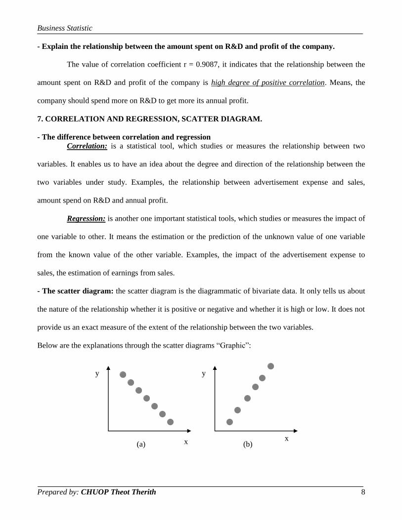
- The scatter diagram: the scatter diagram is the diagrammatic of bivariate data. It only tells us about

the nature of the relationship whether it is positive or negative and whether it is high or low. It does not

provide us an exact measure of the extent of the relationship between the two variables.

Below are the explanations through the scatter diagrams “Graphic”:

x x

y y

(a) (b) x

Business Statistic


1. Picture (a) indicates the correlation is perfect and positive because all the points lie on a

straight line starting from the left bottom and going up towards the right top. It is perfect

positive correlation, means, 100% increase/decrease of x ==> 100% increase/decrease of

y (this case coefficient of correlation is r = +1). Picture (b) indicates the correlation is

perfect and negative because all the points lie on a straight line starting from the left top

and coming down to the right bottom. It is perfect negative correlation, means, 100%

increase/decrease of x ==> 100% decrease/increase of y (this case coefficient of

correlation is r = -1)

2. Picture (c) shows the correlation is positive since this reveals that the values of the two

variables move in the same direction because the plotted points reveal an upward trend

rising from lower left hand corner and going upward to the upper right hand corner. If x

increases/decreases ==> y increases/decreases. Picture (d) shows the correlation is

negative since in this case the values of the two variables move in the opposite direction

because the points depict a downward trend from the upper left hand corner to the lower

right hand corner. If x increases/decreases ==> y decreases/increases.

3. If the points are very dense, i.e., very close to each other, a fairly good amount of

correlation may be expected between the two variables. If the points are widely scattered,

a poor correlation may be expected between them.

y y

x x (c) (d)

x

Business Statistic


8. REGRESSION ANALYSIS

a. Determine the regression equation

Company Sales X

($ millions) Earnings Y ($ millions)

xx yy 2xx 2xx ))(( yyxx

Lucky 89.200 4.900 47.442 -0.442 2250.712 0.195 -20.953

KFC 28.600 6.000 -13.158 0.658 173.142 0.433 -8.663

Mekong Bus 18.200 1.300 -23.558 -4.042 554.995 16.335 95.215

Sorya Bus 69.200 12.800 27.442 7.458 753.045 55.627 204.669

Bayon Bakery 17.500 2.600 -24.258 -2.742 588.467 7.517 66.508

Apsara Bakery 11.900 1.700 -29.858 -3.642 891.520 13.262 108.734

Tiger Beer 71.700 8.000 29.942 2.658 896.503 7.067 79.595

Angkor Beer 58.600 6.600 16.842 1.258 283.642 1.583 21.192

Pizza World 19.600 3.500 -22.158 -1.842 490.992 3.392 40.808

Master Roll 18.600 4.400 -23.158 -0.942 536.308 0.887 21.807

Akira 51.200 8.200 9.442 2.858 89.145 8.170 26.987

Nokia 46.800 4.100 5.042 -1.242 25.418 1.542 -6.260

x

=501.100

y

=64.100

2

xx

=7533.889

2

yy

=116.009

yyxx

=629.641

According to the table above,

641.629

009.116

889.7533

342.512

1.64

758.4112

1.501

2

2

yyxx

yy

xx

N

yy

N

xx

Find the coefficients:

42751.5

009.116

641.629

08357.0889.7533

641.629

22

22

yy

yyxx

dy

dxdyb

xx

yyxx

dx

dxdyb

xy

yx

Business Statistic


Hence,

Equation of line of regression of earnings on sales (y on x):

8513.108357.0

4897.3341.508357.0

)758.41(08357.0341.5

)(

xy

xy

xy

xxbyy yx

Therefore Equation of line of regression of earnings on sales (y on x): y = 0.08357x + 1.8513

Equation of line of regression of sales on earnings (x on y):

766.1242751.5

99195.28758.4142751.5

)342.5(42751.5758.41

)(

yx

yx

yx

yybxx xy

Therefore Equation of line of regression of sales on earnings (x on y): 766.1242751.5 yx

b. Estimate the earnings for a small company with $50.0 million in sales

As equation of line of regression of earnings on sales (y on x): 8513.108357.0 xy so the earnings is

0297.68513.15008357.0 y (in million dollars)

Therefore the earning of that company with $50.0 million in sales is $6.0297 million.

central tendency, dispersion, correlation and regression analysis

Documents