centre for economic performance
TRANSCRIPT

CENTRE FOR ECONOMIC PERFORMANCE
DISCUSSION PAPER NO. 266
October 1995
HOW DOES FINANCIAL PRESSURE AFFECT FIRMS?
Stephen Nickell and Daphne Nicolitsas

ABSTRACT
How does monetary policy work? While one aspect of the investigation has focusedon the behaviour of consumers, another has concentrated on the behaviour ofcompanies faced with the kind of financial pressure associated with tight monetarypolicy. The general focus in this area is on the impact of financial constraints oninvestment expenditures including fixed capital and inventories. Our purpose is toshift this focus somewhat and to concentrate on the impact of financial pressure onother aspects of company behaviour. We first discuss briefly the theoreticalbackground and the empirical formulation. Then, using panel data on a largenumber of UK companies, we derive a number of results.
This paper was produced as part of the Centre'sProgramme on Corporate Performance

HOW DOES FINANCIAL PRESSURE AFFECT FIRMS?
Stephen Nickell and Daphne Nicolitsas
OCTOBER 1995

Published byCentre for Economic Performance
London School of Economics and Political ScienceHoughton Street
London WC2A 2AE
©S.Nickell and D.Nicolitsas
ISBN 0 7530 0229 9

HOW DOES FINANCIAL PRESSURE AFFECT FIRMS?
Stephen Nickell and Daphne Nicolitsas
Page
Introduction 1
1. Theoretical Background 2
2. The Empirical Formulation 4
3. Results 8
Endnotes 12Tables 14Data Appendix 20Table A1 28Table A2 29References 30
The Centre for Economic Performance is financed by the Economic and SocialResearch Council.

ACKNOWLEDGEMENTS
This paper was originally prepared for the CEPR Conference on "InternationalPerspectives on the Microeconomic and Macroeconomic Implications of FinancingConstraints" at the University of Bergamo, October 6-8, 1994. We would like to thankSteve Bond, Robert Cherinko, Glenn Hubbard, Anil Kashyap, Costas Meghir, GerardPfann and Fabio Schiantarelli for helpful comments, and the Economic and SocialResearch Council and the Leverhulme Trust for financial support.

HOW DOES FINANCIAL PRESSURE AFFECT FIRMS?
Stephen Nickell and Daphne Nicolitsas
Introduction
How does monetary policy work? There has been renewed interest in this
question in recent years, sparked by the apparently important role played by
monetary policy in the severe fluctuations in many OECD economies in the last
decade. While one aspect of the investigation has focused on the behaviour of
consumers (see King, 1994, for example), another has concentrated on the behaviour
of companies faced with the kind of financial pressure associated with tight monetary
policy.
A pithy summary of the issues involved is provided in Gertler and Gilchrist
(1993). The general focus in this area is on the impact of financial constraints on
investment expenditures including fixed capital and inventories. We now possess a
large body of microeconometric evidence that liquidity constraints of various kinds
influence investment spending, controlling - at least in part, for current and expected
shifts in product demand.1
Our purpose here is to change this focus somewhat and to concentrate on the
impact of financial pressure on other aspects of company behaviour. We shall
investigate a number of issues. First, do liquidity constraints directly affect
employment as well as investment, again controlling for direct demand shifts?2
Second, in addition to "cutting back", how else do firms respond to financial
pressure? Do they, for example, attempt to negotiate lower wage increases with their
employees? Or do they try and get them to increase productivity by one means or
another? These latter responses will, in fact, offset the potential adverse impact of
financial pressure on employment and investment, by making both activities more
profitable.

2
In order to address these questions, we first discuss briefly the theoretical
background and the empirical formulation. Then, using panel data on a large
number of UK companies, we derive a number of results. These indicate that the
impact of financial pressure on company employment is large and the offsetting
effects on wages and productivity, while detectable, tend to be small.
1. Theoretical Background
In their very useful survey, Gertler and Gilchrist (1993) set out what they describe
as two more or less indisputable facts. First, information asymmetries (between
borrowers and lenders) induce a wedge between the cost of "uncollateralized"
external funds and the price of funds generated by a company internally. Second,
the cost of external funds is increasing not only in the general level of interest rates
but also in the ratio of the size of the loan to "collateralizeable" net worth.
Looking at the first of these, it is clear that even securely collateralized external
funds are likely to be more expensive than internal funds, because of the real costs
involved in evaluating the collateral and monitoring the position of the loan. The
second indisputable fact arises essentially because the probability of bankruptcy rises
when debt rises relative to net worth, and this raises the cost of borrowing because
of the increased risk. Indeed borrowing or credit may even be rationed at some point
but the existence of credit rationing is not necessary to the general argument. Since
a large part of the net worth of a company consists of the present value of future
profits, we can now see how a rise in the general level of interest rates has two
effects on the costs of borrowing for a firm. There is a direct effect because the (safe)
rate of interest has risen and an indirect effect because, as interest rates rise, net
worth falls and so the ratio of debt to net worth rises. The indirect effect, of course,
reinforces the direct effect and is more important the higher is the initial level of debt
(relative to net worth). (See, for example, the discussion in Greenwald and Stiglitz,
1988.)
How will this impact on firms? There are two sorts of impact to consider. First,
there is the direct consequence of the cost of borrowing. Any kind of investment
activity is adversely affected by a rise in borrowing costs, and since these will be

3
more significant when the initial debt position is more adverse, this immediately
implies that the debt position of the company will influence its investment behaviour.
This is confirmed by the results in Bond and Meghir (1994) for fixed capital
investment. The second possible impact relies on the fact that managers' interests are
not the same as shareholders', and that because of informational asymmetries,
managers have some freedom to pursue their interests. These ideas underlie many
conjectures about the behaviour of companies, a good example being the "free cash
flow" theory due to Jensen (1986). In the present context, an important aspect of this
type of analysis is the notion that managers are more concerned by bankruptcy than
are shareholders, basically because the managers have more to lose. So when the
debt position worsens and the threat of bankruptcy looms, managers may not only
cut back on investment of various kinds but may also increase their efforts to cut
costs, raise efficiency, reduce wages and so on. Of course, the very existence of the
"organizational slack" that allows this as a possibility depends on their being a degree
of managerial autonomy in the first place.3
Our investigation here is concerned with a number of these possibilities,
beginning with employment. When borrowing costs rise, investments of all kinds
may be reduced, including the hiring of new employees. Credit restrictions may also
induce a direct contraction of employment by reducing working capital and,
furthermore, the prospective costs of bankruptcy may be reduced if the labour force
is lower. Our main concern here is to investigate the direct impact of financial4
factors on employment controlling for the effect of actual or expected changes in
product demand. This investigation is related to, but is distinct from, that presented
in Sharpe (1994). There, the focus is on how high leverage firms exhibit more
employment responsiveness over the business cycle. Here, we shall be concerned
with actually tracing the consequences of a ceteris paribus increase in financial
pressure on the subsequent behaviour of companies.
Then, as we have already argued, when financial pressure increases, managers
will be very concerned to minimise bankruptcy risks. Workers will also be concerned
if they see their jobs under threat, and this leads naturally to the possibility that
workers and managers will agree both on smaller annual pay increases and on efforts

4
to improve productivity. Both of these will, of course, offset the adverse impact of
financial pressure on investment and employment.
2. The Empirical Formulation
Here we consider the specification of equations which will elucidate the impact
of financial factors on employment, wages and productivity.
Employment
Consider a firm, index i, with a production function
Y = A F(N ,K ) (1)i i i i
where Y = output, N = employment, K = capital, A = efficiency. Then if it sets
prices in an imperfectly competitive environment, the equilibrium level of
employment (ignoring financial factors) is given by
A F (N ,K ) = W (1+t )/P 6 (2)i N i i i 1 i i
where W is the wage, t is the payroll tax rate, P is the price of output and 6 = 1 -i 1 i i
(demand elasticity) . This latter term may systematically vary with current or future−1
expected demand. So if we add in financial factors and dynamics (because of5
adjustment costs), this leads us to investigate a log-linear equation of the form
n = " + " + 8 n + 8 n + " k - " (w -p )it i t 1 it−1 2 it−2 1 it 2 it it
+ " d + " f + , . (3)3 it 4 it it
i refers to company, t to time and " = company effect, " = time effect, n = logi t it
employment, k = log capital, w = log wage, p = log output price,it it it
d = demand terms, f = financial factors. The company effect, " , refers to all thoseit it i
factors (e.g. efficiency) which are company specific but fixed over time. The time
effect, " , captures factors common to all firms such as the payroll tax rate, the safet
rate of interest and so on. Implicit in (3) is an assumption of static expectations.

5
Under non-static expectations, we must also include expected future levels of real
wages and demand. These will be thoroughly investigated in the empirical analysis.
The financial factors which we consider in this and later models are set to capture
the premium on borrowing costs or the probability of credit being rationed
completely. The key variable here is the ratio of debt to "collateralizeable" net worth.
An obvious variable which comes close to capturing this is the ratio of debt to equity.
A typical practical problem here is the fact that while it is easy to obtain the book
value ratio, the market value ratio is much harder to measure correctly. This6
suggests that we consider a flow equivalent, and the most obvious is the ratio of total
interest payments to profits (before tax and interest) plus depreciation. A7
justification for the use of this kind of measure is that if we consider the key variable
to be the ratio of debt to net worth, we could write this as
where D is current debt, B is current profit (including interest payments), r is the safe
interest rate, D is the risk premium, p is the expected rate of inflation and g is the@ e e
expected growth of profits. This ratio can then be written as
Now the first term can arguably be approximated by the ratio of total interest
payments to profits because the average interest payments per unit of debt will
depend on the safe rate and the degree of risk, including a negative element
corresponding to expected growth prospects. The problem with this measure is that
it ignores the second element, namely the fact that part of the interest rate which
corresponds to inflation is effectively being used to pay back the principal.8
Nevertheless this flow measure of financial pressure may well be closer to what is
required than the book value debt-equity ratios, not least because it captures elements
6
of the current cash flow position so beloved of bankers. Indeed, we shall also briefly
consider a third variable precisely because it is one of the bankers' favourite measures
of credit worthiness, namely the "current ratio" which is the ratio of current assets to
current liabilities.9
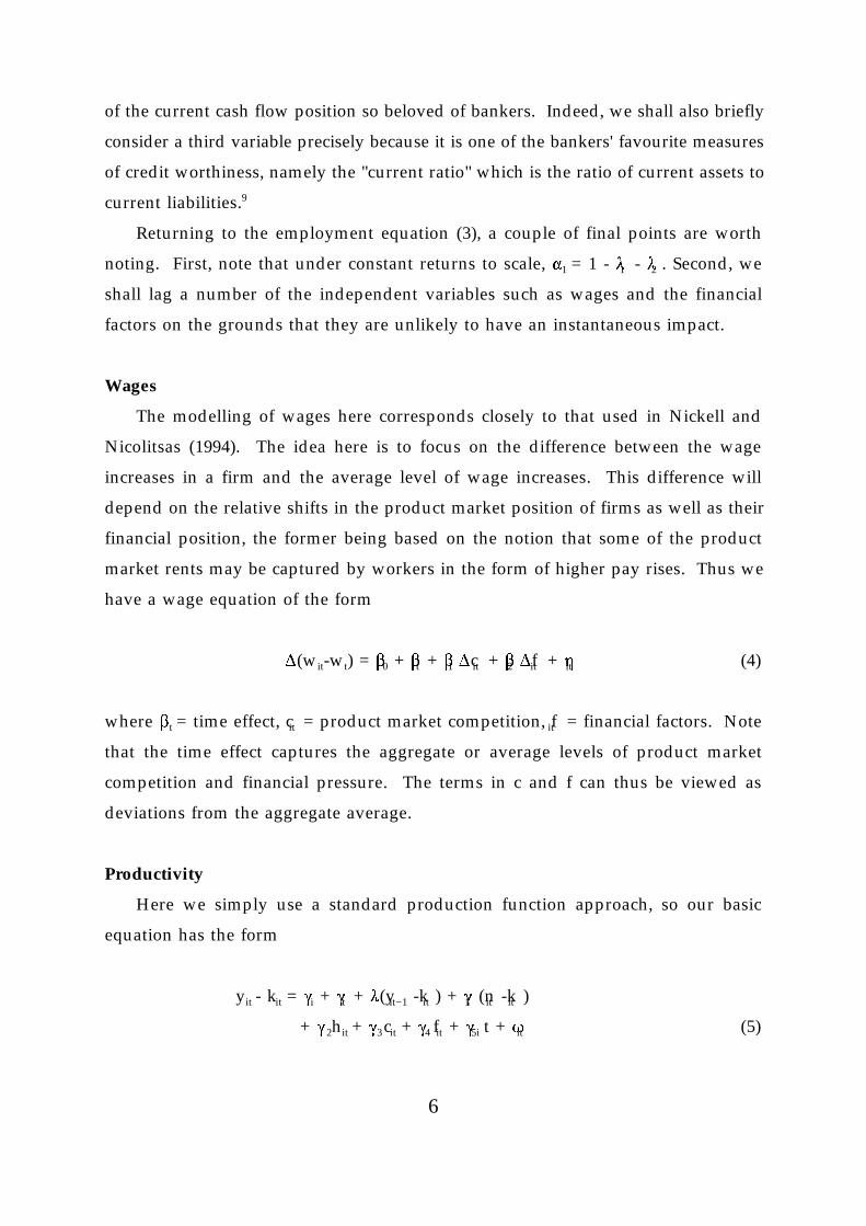
Returning to the employment equation (3), a couple of final points are worth
noting. First, note that under constant returns to scale, " = 1 - 8 - 8 . Second, we1 1 2
shall lag a number of the independent variables such as wages and the financial
factors on the grounds that they are unlikely to have an instantaneous impact.
Wages
The modelling of wages here corresponds closely to that used in Nickell and
Nicolitsas (1994). The idea here is to focus on the difference between the wage
increases in a firm and the average level of wage increases. This difference will
depend on the relative shifts in the product market position of firms as well as their
financial position, the former being based on the notion that some of the product
market rents may be captured by workers in the form of higher pay rises. Thus we
have a wage equation of the form
)(w -w ) = $ + $ + $ )c + $ )f + 0 (4)it t 0 t 1 it 2 it it
where $ = time effect, c = product market competition, f = financial factors. Notet it it
that the time effect captures the aggregate or average levels of product market
competition and financial pressure. The terms in c and f can thus be viewed as
deviations from the aggregate average.
Productivity
Here we simply use a standard production function approach, so our basic
equation has the form
y - k = ( + ( + 8(y -k ) + ( (n -k )it it i t it−1 it 1 it it
+ ( h + ( c + ( f + ( t + T (5)2 it 3 it 4 it 5i it

7
( is a firm effect, ( is a time effect, y = real output, h = cyclical factor based oni t it it
working hours.
So in equation (5) we have a standard constant returns Cobb-Douglas with a
dynamic element to take account of the fact that if new workers join the firm, for
example, it takes some considerable time before they are as proficient and productive
as their more experienced counterparts. The role of product market competition (c)
is to allow for the possibility that competition tends to improve efficiency (see
Nickell, 1993). The financial factors (f) we have already discussed and we also allow
productivity growth to vary systematically across firms via the ( coefficient. This5i
we allow to depend on industry (via 2 digit industry dummies) plus various 3 digit
industry characteristics as well as average firm size.
Data and estimation
The basic data source is the published accounts of around 670 UK manufacturing
companies over the period 1973-86, taken from the EXSTAT data tape. We augment
this with information on a subset of 66 companies from the Confederation of British
Industries (CBI) Wage Settlements survey over the period 1979-86. These data
include information on pay increases for well specified groups of employees and also
whether or not the pay settlement involves the elimination of restrictive labour
practices. The main panel is unbalanced. The number of firms in each year is
available in the Appendix. It peaks in 1980 and then declines rapidly because of
changes in the legal requirements for reporting employment. Detailed definitions of
all the variables may be found in the Appendix.
The employment and productivity models (3), and (5) are specified in levels but
estimated in first differences in order to eliminate the unobserved firm effects. The
wage equation is already in first differences. Generally speaking most current firm
specific variables in these models will have some elements of endogeneity since they
are likely to be influenced by employment, wage and productivity shocks. This
endogeneity extends to the first lag in the first difference context because of the
presence of the lagged error in the equation. The lagged dependent variable is then
automatically endogenous. However, for our present purpose, the most important
endogeneity problems arise with the financial variables. Recall that our key measure

8
of financial pressure is the ratio of interest payments to cash flow which we shall
refer to as the (flow) borrowing ratio. Despite lagging it one period, the danger is
that a lagged shock to employment, caused say by an adverse productivity shock,
will force the firm to increase its borrowings and will subsequently also influence it
directly to change employment. This will generate a spurious correlation between
the lagged borrowing ratio and employment. What we require is a set of instruments
which will impact on the borrowing ratio but have no direct effect on employment.
The instruments we select refer to the performance of the company three years prior
to the employment decision. This will impact on the future borrowing ratio by
influencing its current and hence future debt position but will not influence
employment directly because it is too distant in the past. Recall here that we use a
fixed effects framework so we focus on the time series variation in the data (i.e.
correlating changes with changes) and that we already control for the basic
non-financial factors influencing employment. Furthermore, we are assuming no
serial correlation in the random (non-fixed effect) part of the error, a testable assertion
(see below).
The estimation programme we use was developed by Arrelano and Bond (1991),
and is an efficient extension of the first difference instrumental variables method
suggested for dynamic fixed effects models by Anderson and Hsiao (1981). The
validity of the method depends on the absence of serial correlation in the error
(absence of second order serial correlation in the first difference error) which is
investigated using a robust statistic developed by Arellano and Bond.
3. Results
We begin by looking at some employment regressions which are reported in
Table 1. The reason for reporting a regression using the CBI sample is that the wage
is more accurately measured than in the large sample. In the former case we have
the basic pay for a given number of hours applying to a specific skill group. In the10
large sample, we simply have information on the total wage bill divided by the
number of employees. This measure of pay is corrupted by changes in both hours

9
of work and the skill composition of the workforce as well as measurement error in
employment.
In the first equation reported in Table 1, we have a standard employment
equation with the change in industry output serving as the demand proxy and a flow
measure of leverage, the borrowing ratio (BR). This is the ratio of interest payments
to pre-tax profits with interest payments and depreciation added back in (i.e. cash
flow). We also looked at the debt ratio (DER), that is the ratio of debt to debt plus
equity, both being book value measures. This turns out not to be significant but as
equation 1 reveals, there is some evidence that the borrowing ratio has an
independent effect on employment. In addition, we investigated the impact of the
current ratio (current assets/current liabilities) but it has no important impact either
here or elsewhere, tending to be dominated by the other two variables.
The next five equations in Table 1 are based on a much bigger sample and hence
have more precisely estimated coefficients. The idea of these five equations is to
examine the robustness of the borrowing ratio effect in response to different attempts
to control for current and expected future wages and demand. In equation 3 we
include future wages and industry output, instrumenting these with industry level
forecasts of demand, prices and costs based on the regular surveys published by the
Confederation of British Industry. In equation 4, we treat the future values as
exogenous. Then in equation 5, we include lagged, current and future (real) sales at
the company level treated as endogenous and finally we treat them as exogenous in
equation 6. We recognise that the last three equations are, strictly speaking,
misspecified but we report them simply to see if they reveal any shift in the
borrowing ratio effect. In fact, as Table 1 indicates, the coefficient on the borrowing
ratio remains strongly significant and of the same order of magnitude throughout.
Turning now to Table 2, we investigate some interactions. In columns 1 and 2
we see a slight tendency for the impact of the borrowing ratio to be bigger in firms
with higher levels of debt (relative to equity) and in firms which are relatively
smaller. We also investigated non-linearities, in particular to see whether or not
increases in the borrowing ratio had a bigger impact once the ratio had passed some
threshold. For example, it is said that banks consider that it is prudent for firms to
keep interest payments below a given fraction of profits (e.g. one-quarter). We tried

10
a variety of splines but there was no indication of this effect. Finally, in equation 3,
we see that while the coefficient on the inflation offset to interest payments (pD/B)@
is positively signed, as we might expect, it is both small and insignificant. This
suggests that banks take little or no account of the fact that some of the interest is
actually being used to pay off the debt and should not, therefore, be "counted" as part
of the flow borrowing ratio.
In order to see the orders of magnitude involved in our results, suppose the safe
rate of interest rises from 5 percent to 8 percent (i.e. by 60 percent). Assuming this
implies a 60 percent rise in interest payments, then since the mean value of BR is11
0.2, the effect on BR is an increase of 0.12. Given that the coefficient on BR in Table
1, column 2 is 0.24 this yields a short-run reduction in employment of 2.9 percent.
In the long run this expands to a reduction of around 11 percent. While the rise in
interest rates from 5 to 8 is quite significant, it is by no means exceptional in the
process of tightening monetary policy. So we see that the government can have a12
substantial direct effect on employment by raising interest rates although it takes a
considerable time for the major portion of the effect to come through (e.g two thirds
of the effect takes 5 years). Furthermore, insofar as the firm can enforce a moderation
of wage demands, this will attenuate the employment effect.
Turning now to the impact of financial factors on wage increases, the results
based on equation (4) are reported in Table 3. Both regressions indicate that the flow
borrowing ratio (BR) has some impact on wages. But the effect is not very big. As
we have already noted, a 3 percentage point increase in interest rates from 5 percent
to 8 percent leads to a rise of 0.12 in BR which leads to a short-run reduction in
wages of between 0.2 and 1 percent. The corresponding long-run reduction is around
0.8 percent in equation 1 or 1.6 percent in equation 2. Given that estimated long-run
employment wage elasticities rarely exceed 2.0 (the long-run elasticity in Table 1,
equation 1 is 1.4), this wage reduction is not going to have much of an impact on the
employment effect discussed above, even in the long term (i.e. at most a 3 percent
increase in employment compared to the 11 percent reduction discussed above).
As well as trying to moderate wage bargains, firms under financial pressure may
also attempt to improve efficiency. To capture this effect, in Table 4 we present a
production function estimate based on equation (5). The key result is that the flow

11
borrowing ratio (BR) exhibits a consistent positive effect on (total factor) productivity,
but as with wages, the effect is small. To get some idea of the scale of the effect,
again consider a rise in the interest rate from 5 to 8 percent. This generates an
increase of in total factor productivity of a mere ½ percent in the long run.
Making use of the CBI data set we might be able to gather some information as
to the source of this efficiency improvement. One of the variables reported indicates
whether or not the employees agreed to eliminate restrictive work practices in their
last pay bargain. Since such an event is more or less bound to generate a
productivity improvement, it is worth investigating whether or not the chances of
restrictive practices being eliminated are enhanced if the firm is under financial
pressure. The results are reported in Table 5 and indicate that there may be some
effect from the borrowing ratio in the correct direction (significant at the 10 percent
level) but it is again very small. The usual increase in interest rates from 5 to 8
percent raises the chances of a reduction in restrictive practices by around 1½ percent.
This is, of course, consistent with the small productivity effect. It is worth noting,
however, that there is also an effect from profits per employee which tends to
reinforce the borrowing ratio effect (i.e. a fall in profits raises the chances that
restrictive practices will be removed).
Summary
We have undertaken an investigation of the impact on company behaviour of
increases in financial pressure. Using a flow measure of leverage, interest payments
relative to cash flow, we find that an increase in this variable has a large negative
effect on employment, a fairly small negative effect on pay increases and a small
positive effect on productivity. It also increases the probability that a pay increase
will be associated with the elimination of restrictive labour practices.
The employment coefficients indicate that a rise in interest rates from 5 percent
to 8 percent will generate a short-run employment reduction of nearly 3 percent
which rises to around 11 percent in the long run. The other effects are relatively
small by comparison, although the long-run offset due to lower wages could be as
much as 3 percent.

12
ENDNOTES
1. See, for example, Bond and Meghir (1994); Fazzari et al. (1988); Devereux and
Schiantarelli (1990); Gertler and Gilchrist (1994); Hoshi et al. (1991); and Kashyap et
al. (1994) whose results basically confirm those obtained in the classic study of Meyer
and Glauber (1964). However, the discussion in Chirinko (1994) indicates that some
of this microeconometric evidence is less supportive of finance constraints than is
commonly believed.
2. Earlier results reported in Wadhwani (1987) and Nickell and Wadhwani (1991)
suggest that there may be something in this hypothesis. More recently Sharpe (1994)
finds that high leverage firms have higher employment sales elasticities over the
business cycle (i.e. engage in less labour hoarding). This is obviously consistent with
"liquidity constraints" influencing employment.
3. In the standard, black-box neoclassical model of the firm, costs are minimised by
assumption.
4. Because, for example, employees may be entitled to various forms of
compensation for job loss.
5. The inverse of 6 is the mark-up of price on marginal cost and there is a large andi
inconclusive literature on its cyclical behaviour. See, for example, Bils (1987);
Rotemberg and Saloner (1986); and Layard et al. (1991), Ch. 7.
6. However, it can also be argued that the book value is more exogenous than the
market value so its subsequent impact on employment, say, is easier to interpret.
7. Note this is the inverse of a standard measure of leverage known as the "interest
cover".
8. We shall pursue this issue in the empirical analysis by including an additional
variable in the equation which represents the inflation term (p D/B). @ e

13
9. Current assets include cash, marketable securities, receivables and stocks of
finished goods. If we remove the last, the ratio becomes the "quick" or "acid-test"
ratio.
10. In fact, we have data on the percentage pay increase, but because we estimate
the equation in first differences, this is all we require.
11. Obviously some of a firm's debt has a fixed interest rate but this applies only
to a small proportion.
12. For example, in the final stages of the late 1980s boom, bank base rates rose
from 8.5 percent in 1988 Q1 to 13.0 percent in 1988 Q4.

14
Tab
le 1
Em
plo
ymen
t R
egre
ssio
ns
Con
trol
lin
g fo
r D
eman
d
Dep
end
ent
vari
able
: n i
t
CB
I sa
mpl
eL
arge
sam
ple
('75-
'86)
____
____
____
____
____
____
____
____
____
____
____
____
____
____
____
____
____
____
____
__
'81-
'86
Incl
ude
futu
re v
aria
bles
Incl
ude
firm
out
put
Ind
epen
den
t V
aria
bles
Bas
icB
asic
end
ogen
ous
exog
enou
sen
dog
enou
sex
ogen
ous
12
34
56
*n0.
40(4
.0)
0.89
(11.
8)0.
82(9
.9)
0.82
(10.
4)0.
85(1
1.6)
0.84
(12.
7)it
-1
*n0.
04(0
.5)
-0.1
5(2
.0)
-0.0
8(1
.0)
-0.0
8(1
.2)
-0.0
6(0
.8)
-0.0
6(1
.1)
it-2
*k0.
560.
260.
260.
260.
210.
22it
*w-0
.02
(0.2
)-0
.02
(0.5
)0.
003
(0.0
2)0.
027
(0.7
)it
+1
*)w
-0.2
1(1
.7)
-0.2
6(2
.0)
-0.2
3(1
.9)
-0.2
7(2
.0)
-0.2
4(2
.3)
it
*w-0
.80
(3.1
)-0
.01
(0.1
)-0
.25
(1.7
)-0
.20
(1.5
)-0
.20
(1.5
)-0
.15
(1.3
)it
-1
*y0.
22(1
.4)
0.02
7(0
.4)
0.23
(1.6
)-0
.039
(0.6
)jt+
1
y-0
.06
(0.9
)0.
20(2
.8)
0.27
(3.4
)0.
24(3
.1)
0.14
(1.6
)0.
096
(1.5
)jt y
0.06
(0.9
)-0
.16
(2.2
)-0
.04
(0.5
)-0
.06
(0.9
)0.
02(0
.3)
0.02
(0.4
)jt-
1
*y-0
.03
(0.5
)0.
005
(0.3
)it
+1
*y0.
29(3
.9)
0.31
(10.
1)it
*y-0
.21
(3.3
)-0
.26
(7.6
)it
-1
*Br
-0.0
44(2
.5)
-0.2
4(3
.5)
-0.3
1(4
.1)
-0.3
0(4
.3)
-0.2
6(3
.6)
-0.2
4(3
.7)
it-1
*DE
R-0
.22
(1.2
)-0
.08
(0.4
)-0
.09
(0.5
)-0
.08
(0.5
)-0
.087
(0.5
)it
-1
se0.
078
0.09
10.
088
0.08
80.
078
0.07
7Se
rial
cor
rela
tion
(N
(0,1
))1.
25-0
.048
-0.6
7-0
.55
-1.0
3-0
.98
Inst
rum
ent
valid
ity
P(2
3)=
20.4
P(8
7)=
136.
5P
(80)
=11
5.0
P(8
2)=
116.
8P
(77)
=12
0.6
P(8
2)=
136.
32
22
22
2
Tim
e d
umm
ies
pp
pp
pp
Ind
ustr
y sp
ecif
ic t
rend
sp
pp
pp
pFi
rm d
umm
ies
pp
pp
pp
NT
231
4407
3732
3732
3732
3732
N 6
6 6
75 6
75 6
75 6
75 6
75
15
Tab
le 1
Em
plo
ymen
t R
egre
ssio
ns
Con
trol
lin
g fo
r D
eman
d
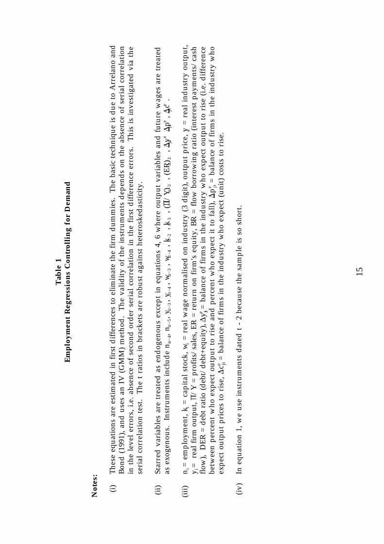
Not
es:
(i
)Th
ese
equa
tions
are
est
imat
ed in
fir
st d
iffe
renc
es t
o el
imin
ate
the
firm
dum
mie
s.
The
basi
c te
chni
que
is d
ue t
o A
rrel
ano
and
Bon
d (
1991
), an
d u
ses
an I
V (
GM
M)
met
hod
. T
he v
alid
ity
of t
he i
nstr
umen
ts d
epen
ds
on t
he a
bsen
ce o
f se
rial
cor
rela
tion
in t
he l
evel
err
ors,
i.e
. abs
ence
of
seco
nd o
rder
ser
ial
corr
elat
ion
in t
he f
irst
dif
fere
nce
erro
rs.
Thi
s is
inv
esti
gate
d v
ia t
hese
rial
cor
rela
tion
tes
t. T
he t
rat
ios
in b
rack
ets
are
robu
st a
gain
st h
eter
oske
das
tici
ty.
(ii)
Star
red
var
iabl
es a
re t
reat
ed a
s en
dog
enou
s ex
cept
in
equa
tion
s 4,
6 w
here
out
put
vari
able
s an
d f
utur
e w
ages
are
tre
ated
as e
xoge
nous
. In
stru
men
ts i
nclu
de
n, n
, y, y
, w, w
, k, k
, (A
/Y
), (
ER
), )
y )
p, )
c.
it−
4it
−5
it−
3it
−4
it−
3it
−4
it−
2it
−3
it−
3it
−3
jtjt
jte
ee
(iii)
n=
empl
oym
ent,
k=
capi
tal
stoc
k, w
= re
al w
age
norm
alis
ed o
n in
dus
try
(3 d
igit
), ou
tput
pri
ce, y
= r
eal
ind
ustr
y ou
tput
,i
i i
j
y=
rea
l fir
m o
utpu
t, A
/Y =
pro
fits/
sale
s, E
R =
ret
urn
on f
irm
's e
quit
y, B
R =
flo
w b
orro
win
g ra
tio
(int
eres
t pa
ymen
ts/
cash
i flow
), D
ER =
deb
t ra
tio (
debt
/deb
t+eq
uity
), )
y=
bal
ance
of
firm
s in
the
ind
ustr
y w
ho e
xpec
t ou
tput
to
rise
(i.e
. dif
fere
nce
jt e
betw
een
perc
ent
who
exp
ect
outp
ut t
o ri
se a
nd p
erce
nt w
ho e
xpec
t it
to
fall)
, )
p=
bal
ance
of
firm
s in
the
ind
ustr
y w
hojt
e
expe
ct o
utpu
t pr
ices
to
rise
, )c
= b
alan
ce o
f fi
rms
in t
he i
ndus
try
who
exp
ect
(uni
t) c
osts
to
rise
.jt
e
(iv
)In
equ
atio
n 1,
we
use
inst
rum
ents
dat
ed t
- 2
bec
ause
the
sam
ple
is s
o sh
ort.

16
Table 2Employment Regressions with Borrowing Ratio Interactions
Dependent variable: nit
BR interaction BR interaction IncludeIndependent Variables with Debt with Size inflation effect
1 2 3
*n 0.82 (9.9) 0.82 (10.1) 0.82 (9.6)it-1
*n -0.08 (1.0) -0.08 (1.0) -0.07 (0.9)it-2
*k 0.26 (0.5) 0.26 0.25it
*w -0.02 (0.2) -0.03 (0.2) -0.02 (0.1)it+1
*)w -0.26 (1.9) -0.26 (2.0) -0.25 (1.9)it
*w -0.25 (1.7) -0.25 (1.7) -0.25 (1.7)it-1
*y 0.22 (1.4) 0.22 (1.4) 0.23 (1.5)jt+1
y 0.28 (3.4) 0.28 (3.4) 0.27 (3.4)jt
y -0.04 (0.5) -0.04 (0.6) -0.04 (0.5)jt-1
*BR -0.32 (3.3)it-1
*(pD/B) 0.03 (0.6)it-1
*BR1D -0.32 (3.4)it-1
*BR2D -0.29 (2.6)it-1
*BR1S -0.27 (2.7)it-1
*BR2S -0.32 (4.0)it-1
*DER -0.08 (0.4) -0.09 (0.5) -0.12 (0.7)it-1
se 0.088 0.087 0.087Serial correlation (N(0.1)) -0.68 -0.73 -0.56
Instrument validity P (79)=114.7 P (79)=114.1 P (79)=114.92 2 2
Time dummies p p pIndustry specific trends p p pFirm dummies p p pNT 3732 3732 3711N 675 675 670
Notes:(i) Starred variables are treated as endogenous. Instruments as in Table 1 (note (ii)).
(ii) Estimation method as in Table 1. Additional variables include pD/B = (absolute) fallein value of debt due to inflation as a proportion of cash flow; BR1D (BR2D) = BR forfirms with above (below) median value of DER; BR1S (BR2S) = BR for firms above(below) median size (as measured by employment).
(iii) Estimation as in Table 1 (note (i)).

17
Table 3Wage Regressions (Dependent variable: )(w -w ))it t
CBI sample ('81-'86) Large sample ('75-'86)Independent Variables 1 2
*)(w -w ) 0.72 (11.0) 0.39 (7.3)it-1 t
)conc -0.043 (1.5) -0.093 (1.9)jt-2
)mksh 0.44 (1.1) 0.62 (3.0)it-2
shock -0.0046 (0.9) -0.016 (1.0)it
*)BR -0.018 (2.1) -0.089 (2.8)it-1
se 0.012 0.062
Serial correlation (N(0,1)) -0.056 -0.46
Instrument validity P (13)=13.0 P (49)=76.42 2
Time dummies p p
NT 231 4113
N 66 618
Notes:
(i) w = nominal wage, w = aggregate nominal wage, conc = industryi j
concentration ratio, mkshi = market share, shock = proportional fall ini i
employment from '79 to '81. The variable is set equal to this fall for the years1982-4 and is set at zero otherwise. BR = flow borrowing ratio.
(ii) Starred variables are treated as endogenous. Additional instruments include
n , n , w , w , y , (B/Y) , ER . See also note (i), Table 1 although in thisit-2 it-3 it-2 it-3 jt it-3 it-3
table, the results are presented in difference form.

18
Table 4
Productivity Regressions (Dependent Variable: y -k )it it
Large sample 1975-86
Independent Variables
*(y -k ) 0.38 (9.6)it-1 it
*(n -k ) 0.62 (11.4)it it
H /H 1.32 (3.9)ojt njt
10 (H /H ) -0.13 (0.5)-3 -1ojt njt
(conc )t -0.038 (2.6)j
(imp )t -0.011 (0.7)j
10 (size )t 0.34 (3.9)-2i
Br 0.030 (1.9)it-2
mksh -1.45 (2.5)it-2
se 0.10
Serial correlation (N(0,1)) -0.14
Instrument validity P (71)=149.12
Firm dummies pTime dummies pIndustry specific trends pNT 4407N 675
Notes:
(i) y = output, k = capital, H = industry overtime hours, H = industry standardi i oj nj
hours, imp = average industry import penetration, average size = average logj
employment, conc = average concentration ratio, BR = flow borrowing ratio,j i
DER = debt ratio, mksh = market share.i i
(ii) Starred variables are treated as endogenous. Additional instruments includey , y , n , n , k , k , (B/Y) (ER) . See also note (i), Table 1.it-2 it-3 it-2 it-3 it-2 it-3 it-3 it-3

19
Table 5Eliminating Restrictive Practices (Dependent variable, )RP)
CBI sample (1981-86)Independent Variables
)mksh -6.71 (2.2)it-2
)(B/N) -0.023 (1.9)it-2
shock 0.27 (1.8)it
)BR 0.12 (1.6)it-1
imp 0.56 (1.9)j
size -0.036 (2.7)i
se 0.28
Serial correlation 1 order(N(0,1)) 0.76st
2 order(N(0,1)) -0.017nd
Time dummies p
Industry dummies p
NT 231
N 66
Notes:
(i) )RP = dummy which takes the value 1 when restrictive practices are reducedi
in the pay round, zero otherwise, mksh = market share, (B/N) = real profiti i
per employee, shock = proportional fall in employment from '79 to '81. Thei
variable is set equal to this fall in the years 1982-4 and is zero otherwise. BRi
= flow borrowing ratio, imp = average industry import penetration, size =j i
average log employment.
(ii) The equation is estimated by OLS but the t ratios are robust to generalheteroskedasticity.

20
DATA APPENDIX
The following datasets are used:
1. The `CBI Sample' consists of longitudinal data on 66 companies over the
period 1979-86 for which we can merge information from the EXSTAT
company database and the Confederation of British Industry (CBI) Pay
Databank. The panel is unbalanced; 10 firms are present for 5 consecutive
years, 7 for 6 years, 8 for 7 and 41 for 8. The first column in Table A2, at the
end of this document, presents the distribution of firms by years.
2. The `Large Sample' consists of longitudinal data on 675 companies for the
period 1972-86 from the EXSTAT company database. The panel is unbalanced
and the distribution of the number of firms by the number of consecutive
years for which they are present is the following:
Years Firms Years Firms
6 112 11 153
7 65 12 15
8 28 13 12
9 51 14 2
10 196 15 41
The second column in Table A2, at the end of this appendix, presents the
distribution of firms across years in this sample. Note that in the wage
regression the sample is reduced to 618 firms since firms for which the Shocki
variable cannot be calculated (i.e. firms which are not present in both 1979 and
1981) have been dropped. It is important to recognise that the reduction in the
sample size after 1981 is not because the relevant firms ceased to exist, merely
that they ceased reporting a consistent measure of employment since they no
longer had any legal requirement to do so.

For the 66 firms in the CBI sample average employment in 1982 is 74131
and median employment is 1764.
21
(A1)
1. Firm-level data
The basic source of the firm-level data are the published company accounts
accessed through the EXSTAT Company Data Service. The definitions of all variables
used and their sources are presented next. Acronyms are presented in brackets next
to the variable descriptions. In general, lower case `versions' of these acronyms,
within the text, refer to the variable in logs.
1. Employment (N )it
Domestic employment (EXSTAT item C15). The firms included in the sample
are fairly large; in 1982 the average employment is 4574 employees and the
median is 961 employees. 1
2. Size (Size )i
This is defined as the average of log employment:
3. Wages (W )it
Two sources for wage information are used:
(a) The published accounts provide information on total domestic
remuneration (EXSTAT item C16). By dividing this by the appropriate
employment figure we get the average total remuneration per
employee. This amount is then converted into real terms by deflating
with the Producer Price Index of the 3-digit industry (see Section 2) to
which the firm belongs.

22
(b) The CBI Pay Databank provides information for a subsample, of 66 out
of the 675 firms, on the pay rise granted for up to 3 bargaining groups.
The pay rise for a manual bargaining group is used here. For this
bargaining group the Databank contains information on:
(i) The month of the pay settlement.
(ii) A manager's estimate of the impact of the settlement on
the gross average earnings in the coming calendar year
and,
(iii) The agreed pay increase.
The last item is not always available. Given, however, that when
available this is nearly always the same as the manager's
estimated increase we use the latter. Information on the month
of the settlement is used to allocate the pay rise over the two
calendar years to which it typically refers (nearly all settlements
last for 12 months).
4. Capital Stock (K )it
This is based on transforming net tangible assets at historic cost into the same
variable at current replacement cost and then normalising on the price index
for plant and machinery. Details of the method are provided in Wadhwani
and Wall (1986).
5. Output (Y )it
Firm sales (EXSTAT item C31) deflated by the producer price index of the
3-digit industry into which the firm belongs.
6. Profits (B )it
Profits before tax (EXSTAT item C34).
7. Effort (RP )it
The existence or otherwise of restrictive practices is used here as a measure of
effort. The CBI Pay Databank provides managers' replies for a subsample, of

23
(A2)
66 out of the 675 firms, on the removal or otherwise of restrictive practices.
The variable is a dummy which takes the value 1 if the reply is affirmative.
The settlement date is used to allocate this variable across the relevant two
calendar years since the removal of restrictive practices is a process lasting for
at least the length of the settlement. In the period 1980-86 around 38 percent
of firms in the sample removed restrictive practices.
_____ 8. Market Share (mksh ) (mksh = 0.011).it it
This is defined as the ratio of firm sales (EXSTAT item C31) over a measure
of industry total sales. Industry total sales (TSALS ) is defined as the productj
of the average number of firms in industry j in a chosen base year (1980) (N )j
with the average sales of a firm in industry j in year t (AVSALS ).jt
The sample of firms used to get the average sales and the number of firms in
each industry contains about 1200 firms including all the major quoted
companies in the industry. The number of firms, N, is held constant to correctj
for the changing composition of the sample.
9. Shock (Shock )i
Shock is defined as the proportional fall in employment from 1979-1981,i
_____that is -(n -n ) (Shock = 0.14).1981 1979 i
____10. Borrowing ratio (BR ) (BR = 0.19).it it

24
(A3)
(A4)
This is defined as:
For those firms for which the denominator in (A3) above takes on a negative
value, that is for firms facing losses prior to the payment of interest rates and
the deduction of depreciation, BR is set equal to 1. Thus BR varies between
0 and 1, its mean value is 0.19 and its median is equal to 0.11. Table A1
presents the average value of BR in each year in the period 1972-1986. The
Borrowing Ratio deteriorated dramatically in 1980 and 1981, consistent with
the decline in profits over the same period, and shows an improvement since
then.
_____11. Debt-Equity ratio (DER ) (DER = 0.52)it it
This is defined as:
As Table A1 indicates, this improved in the 1980s.

25
12. Current Ratio (CURR )it
This is defined as:
Current assets______________Current liabilities
13. Profits over sales (B/Y)
This is the ratio of Profits before tax (EXSTAT item C34) over firm sales
(EXSTAT item C31).
14. Stock Market Returns (ER)
Stock Market returnsare defined as the sum of the dividend received in this
period and the change in the share price as a proportion of the share price in
the last period. That is
where Pt
is the share price in month t and D is the dividend yield att
time t.
The source for this information is the London Business School "London
Share Price Database" (LSPD) and the item is labelled `Log Returns'. The LSPD
contains all companies listed in the London Stock Exchange or in the Unlisted
Securities Market since 1975. Prior to 1975 only a sample of these firms is
reported. LSPD Returns refer to monthly Returns.
Use of Stock Market Returns assumes that the firm is listed in some
market. For firms which are not quoted in either `market' the returns
corresponding to the average of the industry into which they belong have been
used.
The average value of returns over the period 1972-1986 is 18 percent.

26
2. Industry-level variables
1. Producer Price Index (P )jt
Source: British Business and its predecessors and unpublished data from the
Business Statistics Office.
2. Overtime Hours (H )0jt
Weekly overtime hours per operative on overtime times the fraction of
operatives on overtime.
Source: Employment Gazette.
3. Standard Hours (H )njt
Normal weekly hours.
H0jt(mean ____ = 0.07). Hnjt
Source: Employment Gazette.
4. Concentration Ratio (conc )jt
_____Five-firm concentration ratio in terms of sales (conc = 0.41).jt
Source: Annual Report on the Census of Production, Summary Tables,
Table 13.
5. Import Penetration ratio (imp )jt
____Ratio of imports over home demand (sales+imports-exports) (imp = 0.21).jt
Source: Business Monitor MQ12 (collected by S. Machin).
6. Industrial Output (Y )jt
Deflated by Producer Price Index (P ) (see above).jt
Source: Monthly Digest of Statistics.

27
The next 3 variables are forecast variables collected by the CBI in their
Quarterly Industrial Trends Survey. The responses to these questions are
qualitative; only the direction of the expected change has to be reported. The
variable we use is the difference in the proportion of managers expecting a rise
from those expecting a decrease. Data are available at quarterly intervals and
we use the annual average of these. The industry classification adopted by the
CBI is not the same as the Standard Industrial Classification used by official
government statistics. During the period 1972-86 the classification has become
progressively more detailed improving the match between these data and the
firm level data. More specifically the classification has changed twice during
this period; in 1978 and in 1984. The correspondence between the `CBI
Industries' and the Stock Exchange Classification for the periods 1972-77,
1978-83 and 1984-86 are presented in Table 2 below. Note that for the 66 firms
for which we have information from the CBI Pay Databank for the period
1979-1986 the match has been based on the SIC68 information available in the
CBI Pay Databank.
7. Expected change in the volume of output in next 4 months ()y ).j te
8. Expected change in average costs per unit of output ()c ).j te
9. Expected change in the average prices at which domestic orders are booked
()P ).j te
3. Aggregate Variables
1. Wage (W )t
Aggregate wage taken from S. Savouri, `Regional Data 1967-87', Centre for
Economic Performance, London School of Economics, WP No. 133, 1991.

28
Table A1
Financial measures and treasury bill yield in
1972-1986
Year BR Treasury bill DER
yield (%)
1972(422) 0.11 8.48 0.49
1973(435) 0.12 12.82 0.52
1974(450) 0.17 11.30 0.55
1975(494) 0.18 10.93 0.55
1976(649) 0.16 13.98 0.57
1977(669) 0.13 6.39 0.55
1978(664) 0.13 11.91 0.53
1979(664) 0.19 16.49 0.52
1980(660) 0.31 13.58 0.50
1981(620) 0.31 15.39 0.50
1982(307) 0.28 9.96 0.48
1983(125) 0.20 9.04 0.46
1984(102) 0.20 9.33 0.47
1985(88) 0.14 11.49 0.45
1986(83) 0.13 10.94 0.44
Notes:
The numbers in brackets next to the years represent the number of observations from
which the averages have been calculated.
Sources:
1. EXSTAT dataset.
2. Treasury bill yield is from Economic Trends Annual Supplement, 1992 Edition,
Table 47, p.224.

29
Table A2
Number of observations by year
Years `CBI Sample' `Large Sample'
1972 - 422
1973 - 435
1974 - 450
1975 - 494
1976 - 649
1977 - 669
1978 - 664
1979 52 664
1980 55 660
1981 60 620
1982 66 307
1983 65 125
1984 61 102
1985 55 88
1986 39 83

30
References
Anderson, T.W. and Hsiao, C. (1981), "The Estimation of Dynamic Models with Error
Components", Journal of the American Statistical Association, vol. 76, 598-606.
Arrelano, M. and Bond, S.R. (1991), "Some Tests of Specification for Panel Data:
Monte Carlo Evidence and an Application to Employment Equations", Review
of Economic Studies, vol. 58, 277-97.
Bils, M. (1987), "The Cyclical Behaviour of Marginal Cost and Price", American
Economic Review, vol. 77(5), 838-55.
Bond, S. and Meghir, C. (1994), "Dynamic Investment Models and the Firm's Fin
anc
i a l
Pol
i c y
" ,
R e
v i e
w
o f
Eco
n o
mic
Stu
die
s ,
vol.
6 1 (
2 ) ,
197

31
- 2 2
2.
Chirinko, R.S. (1994), "Finance Constraints, Liquidity, and Investment Spending:
Cross-Country Evidence", Research Division, Federal Reserve Bank of Kansas,
RWP 94-05.
Devereux, M. and Schiantarelli, F. (1990), "Investment, Financial Factors and Cash
Flow: Evidence from UK Panel Data", in R.G. Hubbard (ed.), Asymmetric
Information, Corporate Finance and Investment (Chicago: University of
Chicago Press).
Fazzari, S.M., Hubbard, R.G. and Peterson, B.C. (1988), "Financing Constraints and
Corporate Investment", Brookings Papers on Economic Activity, 141-95.
Gertler, M. and Gilchrist, S. (1993), "The Role of Credit Market Imperfections in the
Monetary Transmission Mechanism: Arguments and Evidence", Scandinavian
Journal of Economics, vol. 95(1), 43-64.
Gertler, M. and Gilchrist, S. (1994), "Monetary Policy, Business Cycles, and the
Behaviour of Small Manufacturing Firms", Quarterly Journal of Economics,
CIX, 309-40.
Greenwald, B.C. and Stiglitz, J.E. (1988), "Imperfect Information, Finance Constraints,
and Business Fluctuations", in Meir Kohn and S.C. Tsiang, eds., Finance
Constraints, Expectations and Macroeconomics, Oxford: Oxford University
Press.
Hoshi, T., Kashyap, A. and Scharfstein, D. (1991), "Corporate Structure, Liquidity and
Investment: Evidence from Japanese Industrial Groups", Quarterly Journal of
Economics, vol. 106, 33-60.
32
Jensen, M.C. (1986), "Agency Costs of Free Cash Flow, Corporate Finance and T a
keo
ver
s " ,
A
m e
r i c
a n
Eco
n o
mic
R e
v i e
w ,
P a
per
s
a n
d
Pro
cee
din
g s ,
vol.
7 6 ,
323
- 3 2
9.
Kashyap, A.K., Lamont, O.A. and Stein, J.C. (1994), "Credit Conditions and the
Cyclical Behaviour of Inventories", Quarterly Journal of Economics, CIX,
565-92.

33
King, M. (1994), "Debt Deflation: Theory and Evidence", European Economic Review,
vol. 38, 419-45.
Layard, R., Nickell, S. and Jackman, R. (1991), Unemployment, Macroeconomic
Performance and the Labour Market (Oxford: Oxford University Press).
Meyer, J.R. and Glauber, R.R. (1964), Investment Decisions, Economic Forecasting and
Public Policy (Boston: Harvard University Press)..
Nickell, S. and Nicolitsas, D. (1994), "Wages, Effort and Productivity", Institute of
Economics and Statistics, Oxford University, mimeo.
Nickell, S. and Wadhwani, S. (1991), "Employment Determination in British Industry:
Investigations Using Micro-Data", Review of Economic Studies, vol. 58, 955-69.
Nickell, S. (1993), "Competition and Corporate Performance", Centre for Economic
Performance, London School of Economics, DP No. 182.
Rotemberg, J. and Saloner, G. (1986), "A Super Game Theoretic Model of Price Wars
during Booms", American Economic Review, vol. 76(3), 390-407.
Sharpe, S.A. (1994), "Financial Market Imperfections, Firm Leverage, and the C y
clic
alit
y
o f
Em
plo
y m
ent
" ,
A
m e

34
r i c
a n
Eco
n o
mic
R e
v i e
w ,
vol.
8 4 ,
106
0 - 1
074
.
Wadhwani, S. and Wall, M. (1986), "The UK Capital Stock - New Estimates of Pre
m a
t u r
e
Scr
a p
pin
g " ,
O x
f o r
d
R e
v i e
w
o f
Eco
n o

35
mic
Pol
icy,
vol.
2 ( 3
) ,
4 4 -
55.
Wadhwani, S. (1987), "The Effects of Inflation and Real Wages on Employment",
Economica, vol. 54, 21-40.