centroidal voronoi tessellations applications and algorithms
DESCRIPTION
Centroidal Voronoi Tessellations Applications and AlgorithmsTRANSCRIPT
SIAM REVIEW c© 1999 Society for Industrial and Applied MathematicsVol. 41, No. 4, pp. 637–676
Centroidal Voronoi Tessellations:Applications and Algorithms∗
Qiang Du†
Vance Faber‡
Max Gunzburger§
Abstract. A centroidal Voronoi tessellation is a Voronoi tessellation whose generating points are thecentroids (centers of mass) of the corresponding Voronoi regions. We give some applica-tions of such tessellations to problems in image compression, quadrature, finite differencemethods, distribution of resources, cellular biology, statistics, and the territorial behaviorof animals. We discuss methods for computing these tessellations, provide some analysesconcerning both the tessellations and the methods for their determination, and, finally,present the results of some numerical experiments.
Key words. Voronoi tessellations, centroids, vector quantization, data compression, clustering
AMS subject classifications. 5202, 52B55, 62H30, 6502, 65D30, 65U05, 65Y25, 68U05, 68U10
PII. S0036144599352836
1. Introduction. Given an open set Ω ⊆ RN , the set Viki=1 is called a tessel-
lation of Ω if Vi ∩ Vj = ∅ for i = j and ∪ki=1V i = Ω. Let | · | denote the Euclideannorm on RN . Given a set of points ziki=1 belonging to Ω, the Voronoi region Vicorresponding to the point zi is defined by
Vi = x ∈ Ω | |x − zi| < |x − zj | for j = 1, . . . , k, j = i .(1.1)
The points ziki=1 are called generators. The set Viki=1 is a Voronoi tessellation orVoronoi diagram of Ω, and each Vi is referred to as the Voronoi region correspondingto zi. (Depending on the application, there exist many different names for Voronoi re-gions, including Dirichlet regions, area of influence polygons, Meijering cells, Thiessenpolygons, and S-mosaics.) The Voronoi regions are polyhedra. These tessellations,and their dual tessellations (in R2, the Delaunay triangulations), are very useful in avariety of applications. For a comprehensive treatment, see [47].
∗Received by the editors December 15, 1998; accepted for publication (in revised form) March 3,1999; published electronically October 20, 1999.
http://www.siam.org/journals/sirev/41-4/35283.html†Department of Mathematics, Iowa State University, Ames, IA 50011-2064, and Hong Kong
University of Science and Technology, Clear Water Bay, Kowloon, Hong Kong ([email protected]).The research of this author was supported in part by National Science Foundation grant DMS-9796208 and by grants from HKRGC and HKUST.‡Communications and Computing Division, Los Alamos National Laboratory, Los Alamos, NM
87545. Current address: Lizardtech Inc., 1520 Bellevue Avenue, Seattle, WA 98122 ([email protected]). The research of this author was supported in part by the Department of Energy.§Department of Mathematics, Iowa State University, Ames, IA 50011-2064 (gunzburg@iastate.
edu). The research of this author was supported in part by National Science Foundation grantDMS-9806358.
637

638 QIANG DU, VANCE FABER, AND MAX GUNZBURGER
Fig. 1.1 On the left, the Voronoi regions corresponding to 10 randomly selected points in a square;the density function is a constant. The dots are the Voronoi generators and the circlesare the centroids of the corresponding Voronoi regions. Note that the generators and thecentroids do not coincide. On the right, a 10-point centroidal Voronoi tessellation. Thedots are simultaneously the generators for the Voronoi tessellation and the centroids of theVoronoi regions.
Given a region V ⊆ RN and a density function ρ, defined in V , the mass centroidz∗ of V is defined by
z∗ =
∫V
yρ(y) dy∫V
ρ(y) dy.(1.2)
Given k points zi, i = 1, . . . , k, we can define their associated Voronoi regionsVi, i = 1, . . . , k. On the other hand, given the regions Vi, i = 1, . . . , k, we can definetheir mass centroids z∗i , i = 1, . . . , k. Here, we are interested in the situation where
zi = z∗i , i = 1, . . . , k,(1.3)
i.e., the points zi that serve as generators for the Voronoi regions Vi are themselvesthe mass centroids of those regions. We call such a tessellation a centroidal Voronoitessellation. This situation is quite special since, in general, arbitrarily chosen pointsin RN are not the centroids of their associated Voronoi regions. See Figure 1.1 for anillustration in two dimensions.
One may ask, How does one find centroidal Voronoi tessellations, and are they ofany use? In this paper, we review some answers to these questions. Concerning thefirst question, and to be more precise, consider the following problem:
Givena region Ω ⊆ RN ,a positive integer k, anda density function ρ, defined for y in Ω,
findk points zi ∈ Ω andk regions Vi that tessellate Ω
such that simultaneously for each i,
CENTROIDAL VORONOI TESSELLATIONS 639
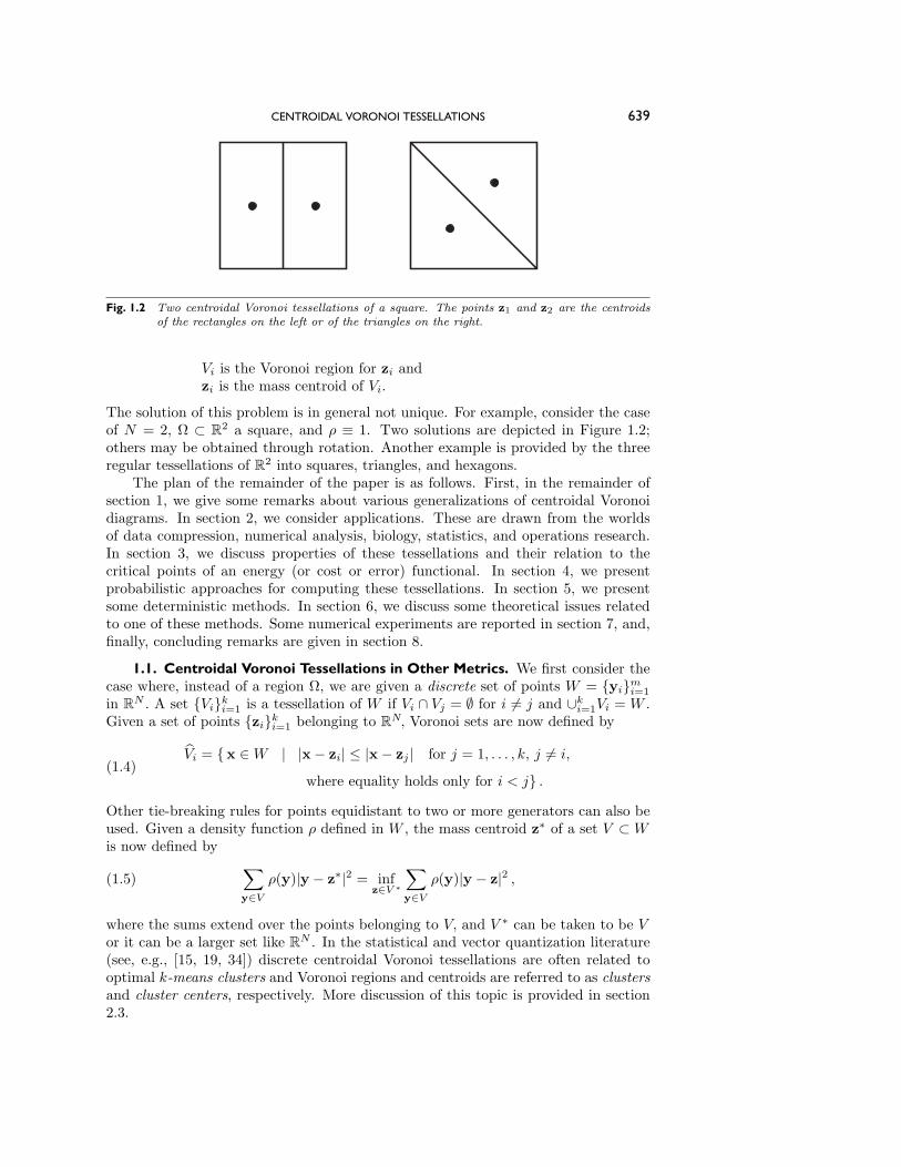
Fig. 1.2 Two centroidal Voronoi tessellations of a square. The points z1 and z2 are the centroidsof the rectangles on the left or of the triangles on the right.
Vi is the Voronoi region for zi andzi is the mass centroid of Vi.
The solution of this problem is in general not unique. For example, consider the caseof N = 2, Ω ⊂ R
2 a square, and ρ ≡ 1. Two solutions are depicted in Figure 1.2;others may be obtained through rotation. Another example is provided by the threeregular tessellations of R2 into squares, triangles, and hexagons.
The plan of the remainder of the paper is as follows. First, in the remainder ofsection 1, we give some remarks about various generalizations of centroidal Voronoidiagrams. In section 2, we consider applications. These are drawn from the worldsof data compression, numerical analysis, biology, statistics, and operations research.In section 3, we discuss properties of these tessellations and their relation to thecritical points of an energy (or cost or error) functional. In section 4, we presentprobabilistic approaches for computing these tessellations. In section 5, we presentsome deterministic methods. In section 6, we discuss some theoretical issues relatedto one of these methods. Some numerical experiments are reported in section 7, and,finally, concluding remarks are given in section 8.
1.1. Centroidal Voronoi Tessellations in Other Metrics. We first consider thecase where, instead of a region Ω, we are given a discrete set of points W = yimi=1in RN . A set Viki=1 is a tessellation of W if Vi ∩ Vj = ∅ for i = j and ∪ki=1Vi = W .Given a set of points ziki=1 belonging to R
N, Voronoi sets are now defined by
Vi = x ∈W | |x − zi| ≤ |x − zj | for j = 1, . . . , k, j = i,where equality holds only for i < j .
(1.4)
Other tie-breaking rules for points equidistant to two or more generators can also beused. Given a density function ρ defined in W , the mass centroid z∗ of a set V ⊂Wis now defined by ∑
y∈Vρ(y)|y − z∗|2 = inf
z∈V ∗∑y∈V
ρ(y)|y − z|2 ,(1.5)
where the sums extend over the points belonging to V, and V ∗ can be taken to be Vor it can be a larger set like RN . In the statistical and vector quantization literature(see, e.g., [15, 19, 34]) discrete centroidal Voronoi tessellations are often related tooptimal k-means clusters and Voronoi regions and centroids are referred to as clustersand cluster centers, respectively. More discussion of this topic is provided in section2.3.
640 QIANG DU, VANCE FABER, AND MAX GUNZBURGER
The notions of Voronoi regions and centroids, and therefore of centroidal Voronoiregions, may be generalized to more abstract spaces and to metrics other than theEuclidean 2-norm. For example,
d(x,y) = ‖x − y‖pp(1.6)
will be of interest to us. For another example, let d(x,y) denote a distance functioninduced by a norm that is equivalent to the l2 norm on RN . Let ≺ be an order ofRN . Then, Voronoi tessellations of Ω, with respect to this metric, are defined by
Vi = x ∈ Ω | d(x, zi) < d(x, zj), j = 1, . . . , k, j = i , andd(x, zi) = d(x, zj), j ≺ i .
(1.7)
Notice that, without the inclusion of the part d(x, zi) = d(x, zj), Vi does not nec-essarily provide a partition of Ω, as there could be nonempty boundaries. Using apartial order, one may decide how portions of boundaries with nonempty interiorsget assigned to specific Voronoi regions. Such a partition, in general, only guaranteesthat the Voronoi regions are star shaped (with respect to the metric) [37].
Note that if one instead considers
Vi = x ∈ Ω | d(x, zi) ≤ d(x, zj), j = 1, . . . , k, j = i ,(1.8)
then the regions may overlap but they remain convex.A generalized definition of the centroid z∗ of a region V with respect to a density
function ρ might be given by∫V
ρ(y)d(z∗,y) dy = infz∈V ∗
∫V
ρ(y)d(z,y) dy .(1.9)
Here, V ∗ can be the closure of V or the region defined by (1.8) or even RN so long asthe existence of z∗ can be guaranteed by either the compactness or the convexity ofthe region and by the convexity of the functional. Centroidal Voronoi tessellations ofΩ can again be defined by (1.3).
One may generalize (1.9) even further to∫V
ρ(y)f(d(z∗,y)) dy = infz∈V ∗
∫V
ρ(y)f(d(z,y)) dy(1.10)
for some function f such that f(d(z∗ − y)) is convex in y.The notion of Voronoi regions may be extended to weighted Voronoi regions [30]
and to more abstract spaces, and the generators can also be lines, areas, or othermore abstract objects [47]. In addition, the metrics need not be induced by a norm.
2. Applications. In this section, we provide a number of applications of cen-troidal Voronoi tessellations.
2.1. Data Compression in Image Processing. The first application is to datacompression. We will use a context from image processing; however, the basic ideasand principles are valid for many other data compression applications.
The setting is as follows. We have a color picture composed of many pixels, eachof which has an associated color. Each color is a combination of basic colors such asred, green, and blue. Let the components of y represent a possible combination ofthe basic colors, and let ρ(y) denote the number of times the particular combinationy occurs in the picture. We let W denote the set of admissible colors, i.e., the set

CENTROIDAL VORONOI TESSELLATIONS 641
of allowable combinations of the basic colors. In a given picture, there may be manydifferent colors. For example, there may be on the order of 106 pixels in a picture,with each pixel potentially having a different color. Our task is to approximate thepicture by replacing the color at each pixel by one from a smaller set of colors ziki=1,where each zi ∈ W . For related discussions, we refer to [24, 25, 32]. In particular, adiscussion of different clustering algorithms in image compression applications can befound in [24].
We give a concrete example. Suppose the picture is composed of 106 pixels andthe color at each pixel is determined by a 24-bit number. (We could, for example,have 8 bits each for the intensity of red, green, and blue.) Then, the cardinality ofW is 224 and the amount of information necessary to describe the picture is 106 × 24bits. Now, suppose we approximate the picture using only 8-bit colors, so that nowwe will use only 256 = 28 possible colors. We still have 106 pixels, so that the amountof information needed to describe the approximate picture is 106 × 8 bits, a reductionof 1/3. Note that we are reducing the amount of data not by reducing the number ofpixels but by reducing the amount of information associated with each pixel.
A natural question is how one assigns the colors in the original picture to thecolors in the set ziki=1. The shell of such an algorithm is given as follows:
Giventhe set of admissible colors W,a positive integer k, anda density function ρ defined in W,
choosek colors zi belonging to W andk sets Vi that tessellate W ,
thenif y is a color appearing in the original picture and y ∈ Vi, replace ywith zi.
(A tie-breaking algorithm must be appended in case y belongs to the boundary ofone of the sets Vi.)
The definition of this algorithm is completed once one specifies how to choosethe sets ziki=1 and Viki=1. Clearly, one would want to choose these sets so thatthe approximate picture using only k colors is a “good” approximation to the givenpicture that contains many more colors.
In a straightforward way, one may use aMonte Carlomethod, using ρ(y) (suitablynormalized) as a probability density, to choose the set of approximating colors ziki=1.Once this set is determined, it is natural to choose the assignment sets Viki=1 to bethe associated Voronoi sets. Unfortunately, even with k = 256, the approximatepictures produced in this manner are not always satisfactory.
A better approximate picture is found if the sets ziki=1 and Viki=1 are chosenso that the functional
E((zi, Vi), i = 1, . . . , k) = k∑i=1
∑yj∈Vi
ρ(yj)|yj − zi|2(2.1)
is minimized over all possible sets of k points belonging to W = yimi=1 and allpossible tessellations ofW into k regions Vi, i = 1, . . . , k. Note that no a priori relationbetween the points zi and subsets Vi is assumed. The motivation for minimizing Eis clear: one is then minimizing the sum of the squares of the distances, in the color

642 QIANG DU, VANCE FABER, AND MAX GUNZBURGER
Fig. 2.1 An 8-bit monochrome picture (top left) and the compressed 3-bit images by the Monte Carlosimulation (top right), the centroidal Voronoi algorithm (bottom left), and the centroidalVoronoi algorithm with dithering (bottom right).
space W and weighted by the density function ρ(y), between the colors yj in thepicture and the reduced color set zi. It is important to note that the minimizationprocess is both over all possible subsets ziki=1 of reduced colors and, independently,over all possible subsets Viki=1 that tessellateW, the only restriction being that bothsets have cardinality k.
In section 3, we shall show that E is minimized when the Vi’s are the Voronoisets for the zi’s and, simultaneously, the zi’s are the mass centroids of the Vi’s, inthe sense of (1.3) and (1.4), respectively. In other words, the zi’s and Vi’s form acentroidal Voronoi tessellation with respect to the density function ρ(y). Note thatthe centroidal Voronoi property is a necessary (but in general not sufficient) optimalitycondition; see the discussion related to Figure 6.1 in section 6.1.
The same principle can be applied to the compression of monochrome pictures.In Figure 2.1, we give an original 8-bit monochrome picture (top left), an approximate3-bit compressed image determined by a Monte Carlo algorithm (top right), and anapproximate 3-bit compressed image determined by a centroidal Voronoi algorithm(bottom left). Clearly, the centroidal Voronoi algorithm results in a better approxi-mate picture. (Of course, there are other image-data compression algorithms that aremore effective than the Monte Carlo algorithm; again, see, e.g., [24] for discussionsand comparisons.)
The compressed image obtained by the centroidal Voronoi algorithm suffers froma phenomenon known as contouring; see the shoulder in the image on the bottom

CENTROIDAL VORONOI TESSELLATIONS 643
left of Figure 2.1. We emphasize that contouring is a difficulty associated with theassignment step of the algorithm and not with the particular choice for the reduced setof colors. Contouring occurs when the colors (or, in the case of a monochrome picture,the shades of gray) in the original, uncompressed picture are changing “continuously.”Then, the colors (or shades) of two neighboring pixels in the physical picture can be onopposite sides of an edge of a Voronoi region in color space. As a result, two differentcolors (or shades) are assigned to the two neighboring pixels so that the distributionof colors in the compressed picture becomes discontinuous, e.g., contours appear inthe image.
Contouring can be ameliorated by dithering. For example, instead of alwaysassigning a color to the nearest color in the reduced set, i.e., to the generator ofthe Voronoi region to which the color belongs, one sometimes assigns a color to thesecond-nearest generator. The assignments can be done based on the relative distancesfrom the point to be assigned to the two nearest generators. Then, if these distancesare nearly equal, i.e., if the point is near the boundary of its Voronoi polygon incolor space, it is almost as probable that the point will be assigned to the secondnearest generator. On the other hand, if the point is near its Voronoi generator, itis much more probable that it will be assigned to that point. If d1 and d2 denotethe distances in color space between the point to be assigned and the nearest andsecond nearest Voronoi generators, respectively, one simple aproach is to assign thepoint to the nearest generator with probability d2/(d1+d2) and to the second nearestgenerator with probability d1/(d1+d2). The bottom right image in Figure 2.1 is thatof a compressed image determined using the same centroidal Voronoi tessellation forthe approximating shades of gray as was used for the bottom left picture, but forwhich the assignment is done by this dithering algorithm. The contours have nowdisappeared.
2.2. Optimal Quadrature Rules. For a given region Ω ⊂ RN and a given positiveinteger k, consider quadrature rules of the type∫
Ωf(y) dy ≈
k∑i=1
Aif(zi) ,
where ziki=1 are k points in Ω and Aiki=1 are the volumes of a set of regions Viki=1that tessellate Ω. We would like to choose the zi’s and Vi’s so that the quadraturerule is, in some sense, as accurate as possible.
Let us examine the quadrature error for the class of Lipschitz continuous functionsf(y) with, say, Lipschitz constant L. In this case, we have that the quadrature errorQ is given by
Q =∣∣∣∣ ∫
Ωf(y) dy −
k∑i=1
Aif(zi)∣∣∣∣
=∣∣∣∣ k∑i=1
∫Vi
(f(y)− f(zi)
)dy∣∣∣∣ ≤ L k∑
i=1
∫Vi
|y − zi| dy .(2.2)
Thus, it is natural to try to choose ziki=1 and Viki=1 so that the right-hand side of(2.2) is minimized.
We may also consider quadrature rules that use the values of the function f andits first p− 1 derivatives evaluated at the points zi. Then, if the (p− 1)st derivativeof f is Lipschitz continuous with Lipschitz constant L, we have that the quadrature

644 QIANG DU, VANCE FABER, AND MAX GUNZBURGER
error Q is now estimated by
Q ≤ Lk∑i=1
∫Vi
|y − zi|p dy .(2.3)
Again, it is natural to try to choose ziki=1 and Viki=1 so that the right-hand sideof (2.3) is minimized.
The minimization of the right-hand side of (2.2) or (2.3) is accomplished whenthe Vi’s are the Voronoi sets for the zi’s and, simultaneously, the zi’s are the masscentroids of the Vi’s, in the sense of (1.7)–(1.9), where d(·, ·) is given by (1.6). Thismay be shown using techniques similar to the ones discussed in section 3.
The problem of finding an optimal numerical quadrature rule has been well stud-ied in the literature. For instance, the classical Gaussian integration rules [7] and thequasi–Monte Carlo rules based on number-theoretic methods all share optimal prop-erties in some sense. We refer to [46] for a comprehensive treatment of the lattersubject; see also [26, 49, 57] for some recent developments. In general, one can con-sider optimal quadrature rules over a given function space and for specific types offunction evaluations. The appearance of the centroidal Voronoi diagrams is the resultof the special function spaces we have chosen here. We note that for integrals overirregular domains, many sophisticated integration rules can provide estimates supe-rior to that for centroidal Voronoi diagrams, but the former require partitioning ormapping into regular regions. On the other hand, the quadrature rules given by thecentroidal Voronoi diagrams can be a convenient method to provide a crude estimatewith very limited information known about the integrand.
2.3. Optimal Representation, Quantization, and Clustering. A related appli-cation is the representation or interpolation of observed data. For example, in one ofthe earliest practical applications of Voronoi diagrams, Thiessen studied the problemof estimating the total precipitation in 1911 in a given geographical region. The math-ematical problem can be described as follows. Given k locations of the pluviometersxi and associated subregions Vi, if p(xi) denotes the precipitation at xi, then thetotal precipitation
P =k∑i=1
∫Vi
p(x) dx
can be estimated byk∑i=1
p(xi)|Vi| ,
where |Vi| denotes the area of Vi. If we wish to find the best locations for the plu-viometers in order to reduce the estimation error, we may follow the discussion insection 2.2 to formulate this optimization problem as an optimal quadrature prob-lem. Another formulation is documented in [47]. Imagine that the function p(x) is arandom variable at x which can be expressed as
p(x) = m(x) + ε(x) ,
where m(x) is a deterministic continuous function of x and ε(x) is a random functionhaving zero expected value. Then, the estimation error can be formulated as
E(xi, i = 1, . . . , k) = E[
k∑i=1
∫Vi
|p(x)− p(xi)|2 dx].

CENTROIDAL VORONOI TESSELLATIONS 645
In the case of constant variance E[ε(x)2] = σ, and if the change in m(x) is smallcompared with the variance σ in the associated region, one can approximate the aboveerror by
E(xi, i = 1, . . . , k) = k∑i=1
∫Vi
2σ2(1− Cov(x,xi)) dx .
Here, Cov(x,xi) is the covariance. Empirically, 1− Cov(x,xi) may be treated as anincreasing function f(|x − xi|) of the distance |x − xi|; thus, the problem of findingthe optimal locations for pluviometers can be formulated as the minimization of thefunctional
E(xi, i = 1, . . . , k) = 2σ2k∑i=1
∫Vi
f(|x − xi|) dx,
which is, again, a problem of finding the centroidal Voronoi diagram.A similar and even earlier example is the question of round-off, i.e., representing
real numbers by the closest integers. This problem has been studied in [56] and theanswer is obviously a simple example of one-dimensional centroidal Voronoi diagrams.
The representation of a given quantity with less information is often referred toas quantization and it is an important subject in information theory. The subject ofvector, i.e., multidimensional, quantization has broad applications in signal process-ing and telecommunications. The image compression example we discussed earlierbelongs to this subject as well. We refer to [15, 17] for surveys on the subject andcomprehensive lists of references to the literature; see also [16].
In the same spirit, centroidal Voronoi diagrams also play a central role in clus-tering analysis; see, e.g., [19, 34, 54]. Clustering, as a tool to analyze similarities anddissimilarities between different objects, is fundamental and is used in various fieldsof statistical analysis, pattern recognition, learning theory, computer graphics, andcombinatorial chemistry. Given a set W of objects, the aim is to partition the setinto, say, k disjoint subsets, called clusters, that best classify the objects accordingto some criteria that distinguishes between them. This is commonly referred to ask-clustering analysis. For example, in combinatorial chemistry, k-clustering analysisis used in compound selection [6], where the similarity criteria may be related to thecompound components as well as their structure. Clustering analysis provides a se-lection of a finite collection of templates that well represent, in some sense, a largecollection of data. To illustrate the connection between centroidal Voronoi diagramsand the optimal k-clustering, let us consider a simple example where W contains mpoints in RN . Given a subset (cluster) V of W with n points, the cluster is to berepresented by the arithmetic mean
xi =1n
∑xj∈V
xj ,(2.4)
which corresponds to the mass centroid of V in the definition (1.5) with V ∗ = RN .The variance is given by
V ar(V ) =∑
xj∈V|xj − x|2,
and for a k-clustering Viki=1 (a tessellation of W into k disjoint subsets), the total
646 QIANG DU, VANCE FABER, AND MAX GUNZBURGER
variance is given by
V ar(W ) =k∑i=1
V ar(Vi) =k∑i=1
∑xj∈Vi
|xj − xi|2 .(2.5)
As observed in [24, 30], the optimal k-clustering having the minimum total varianceoccurs when Viki=1 is the Voronoi partition of W with xiki=1 as the generators;i.e., the optimal k-clustering is a centroidal Voronoi diagram if we use the abovevariance-based criteria.
In computational geometry, criteria such as the diameter or radius of the subsetshave been well studied; see, e.g., [2]. Other criteria have also been proposed, e.g.,L1 based [25] and variance based [62]. In some applications of statistical analysis,only the clusters are of interest; the cluster centers are not important themselves. Inother applications, e.g., the color image compression problem, the cluster centers arethe representative colors to be retained; i.e., they should be elements of W . Thus, itmay be more appropriate to replace the simple arithmetic mean by the more generalnotion of the mass centroid given in section 1.1. For discussions of complexity issuesinvolved in k-clustering as well as related clustering algorithms, see [12, 30, 32, 31, 48]and the references cited therein. Additional references on clustering analysis are alsoprovided in later sections.
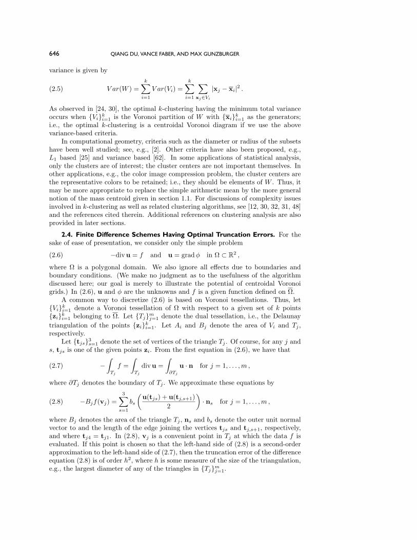
2.4. Finite Difference Schemes Having Optimal Truncation Errors. For thesake of ease of presentation, we consider only the simple problem
−divu = f and u = gradφ in Ω ⊂ R2 ,(2.6)
where Ω is a polygonal domain. We also ignore all effects due to boundaries andboundary conditions. (We make no judgment as to the usefulness of the algorithmdiscussed here; our goal is merely to illustrate the potential of centroidal Voronoigrids.) In (2.6), u and φ are the unknowns and f is a given function defined on Ω.
A common way to discretize (2.6) is based on Voronoi tessellations. Thus, letViki=1 denote a Voronoi tessellation of Ω with respect to a given set of k pointsziki=1 belonging to Ω. Let Tjmj=1 denote the dual tessellation, i.e., the Delaunaytriangulation of the points ziki=1. Let Ai and Bj denote the area of Vi and Tj ,respectively.
Let tjs3s=1 denote the set of vertices of the triangle Tj . Of course, for any j and
s, tjs is one of the given points zi. From the first equation in (2.6), we have that
−∫Tj
f =∫Tj
divu =∫∂Tj
u · n for j = 1, . . . ,m ,(2.7)
where ∂Tj denotes the boundary of Tj . We approximate these equations by
−Bjf(vj) =3∑s=1
bs
(u(tjs) + u(tj,s+1)
2
)· ns for j = 1, . . . ,m ,(2.8)
where Bj denotes the area of the triangle Tj , ns and bs denote the outer unit normalvector to and the length of the edge joining the vertices tjs and tj,s+1, respectively,and where tj4 = tj1. In (2.8), vj is a convenient point in Tj at which the data f isevaluated. If this point is chosen so that the left-hand side of (2.8) is a second-orderapproximation to the left-hand side of (2.7), then the truncation error of the differenceequation (2.8) is of order h2, where h is some measure of the size of the triangulation,e.g., the largest diameter of any of the triangles in Tjmj=1.
CENTROIDAL VORONOI TESSELLATIONS 647
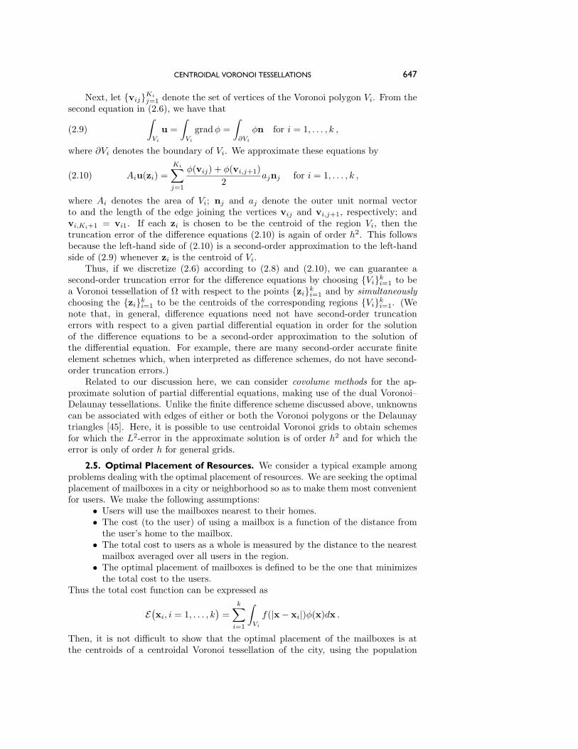
Next, let vijKij=1 denote the set of vertices of the Voronoi polygon Vi. From thesecond equation in (2.6), we have that∫
Vi
u =∫Vi
gradφ =∫∂Vi
φn for i = 1, . . . , k ,(2.9)
where ∂Vi denotes the boundary of Vi. We approximate these equations by
Aiu(zi) =Ki∑j=1
φ(vij) + φ(vi,j+1)2
ajnj for i = 1, . . . , k ,(2.10)
where Ai denotes the area of Vi; nj and aj denote the outer unit normal vectorto and the length of the edge joining the vertices vij and vi,j+1, respectively; andvi,Ki+1 = vi1. If each zi is chosen to be the centroid of the region Vi, then thetruncation error of the difference equations (2.10) is again of order h2. This followsbecause the left-hand side of (2.10) is a second-order approximation to the left-handside of (2.9) whenever zi is the centroid of Vi.
Thus, if we discretize (2.6) according to (2.8) and (2.10), we can guarantee asecond-order truncation error for the difference equations by choosing Viki=1 to bea Voronoi tessellation of Ω with respect to the points ziki=1 and by simultaneouslychoosing the ziki=1 to be the centroids of the corresponding regions Viki=1. (Wenote that, in general, difference equations need not have second-order truncationerrors with respect to a given partial differential equation in order for the solutionof the difference equations to be a second-order approximation to the solution ofthe differential equation. For example, there are many second-order accurate finiteelement schemes which, when interpreted as difference schemes, do not have second-order truncation errors.)
Related to our discussion here, we can consider covolume methods for the ap-proximate solution of partial differential equations, making use of the dual Voronoi–Delaunay tessellations. Unlike the finite difference scheme discussed above, unknownscan be associated with edges of either or both the Voronoi polygons or the Delaunaytriangles [45]. Here, it is possible to use centroidal Voronoi grids to obtain schemesfor which the L2-error in the approximate solution is of order h2 and for which theerror is only of order h for general grids.
2.5. Optimal Placement of Resources. We consider a typical example amongproblems dealing with the optimal placement of resources. We are seeking the optimalplacement of mailboxes in a city or neighborhood so as to make them most convenientfor users. We make the following assumptions:
• Users will use the mailboxes nearest to their homes.• The cost (to the user) of using a mailbox is a function of the distance fromthe user’s home to the mailbox.
• The total cost to users as a whole is measured by the distance to the nearestmailbox averaged over all users in the region.
• The optimal placement of mailboxes is defined to be the one that minimizesthe total cost to the users.
Thus the total cost function can be expressed as
E(xi, i = 1, . . . , k) = k∑i=1
∫Vi
f(|x − xi|)φ(x)dx .
Then, it is not difficult to show that the optimal placement of the mailboxes is atthe centroids of a centroidal Voronoi tessellation of the city, using the population

648 QIANG DU, VANCE FABER, AND MAX GUNZBURGER
density φ as a density function and f(z) = z2. For other choices of f , we also get thecentroidal Voronoi tessellation in the generalized sense. More details can be found in,e.g., [33, 47].
The same formulation can be generalized to other problems related to the optimalplacement of resources, such as schools, distribution centers, mobile vendors, busterminals, voting stations, and service stops.
2.6. Cell Division. There are many examples of animal and plant cells, usu-ally monolayered or columnar, whose geometrical shapes are polygonal. In manycases, they can be identified with a Voronoi tessellation and, indeed, with a centroidalVoronoi tessellation; see, e.g., [27, 28] for examples. Likewise, centroidal Voronoitessellations can be used to model how cells are reshaped when they divide or areremoved from a tissue. Here we consider one example provided in [27, 28], namely,cell division in certain stages in the development of a starfish (Asteria pectinifera)embryo. During this stage, the cells are arranged in a hollow sphere consisting of asingle layer of columnar cells. It is shown in [27, 28] that, viewed locally along thesurface, the cell shapes closely match that of a Voronoi tessellation and, in fact, arethat of a centroidal Voronoi tessellation.
The results of the cell division process can also be described using centroidalVoronoi tessellations; see [27, 28]. We start with a configuration of cells that, byobservation, is a Voronoi tessellation. In this geometrical description of the cell shapes,cell division can be modeled as the addition of another Voronoi generator or, moreprecisely, as the splitting of a Voronoi generator into two generators. Having added agenerator (or more than one if more than one cell divides), how does one determinethe shapes of the new cells and the (necessarily) different shapes of the remaining oldcells? In [27, 28] it is shown that the new shapes are very closely approximated by acentroidal Voronoi tessellation corresponding to the increased number of generators.
The exact geometrical cell division algorithm described in [27, 28] is as follows. Aphotograph of an arrangement of polygonal cells is shown to be closely approximatedby a Voronoi tessellation and is used to define data from which the correspondingVoronoi generators are determined. Additional photographs (taken at later times)are used to identify the parent cells that divide. The generator of a parent cell (nowrepresented by a Voronoi polygon) is replaced by two points lying along a long axisof the cell; the exact placement of the two points turns out to be unimportant. Anew Voronoi tessellation is determined using the generators of the cells that havenot divided along with the points resulting from the replacement of the generators ofthe parent cells. In this manner, two daughter cells are introduced for each parentcell. The shapes of these cells are now adjusted by first moving all the generatorsto the centroids of their corresponding Voronoi polygon and then recomputing theVoronoi tessellation. This procedure is repeated until the cell shapes, i.e., the Voronoipolygons, cease to change. The final arrangement of cells determined by this iterativeprocess is a centroidal Voronoi tessellation (see section 5.2) and matches very wellwith photographs of the actual cells after the cell division process is completed.
2.7. Territorial Behavior of Animals. Many species of animals employ Voronoitessellations to stake out territory. If the animals settle into a territory asynchronously,i.e., one or a few at a time, the distribution of Voronoi generators often resembles thecenters of circles with fixed radius in a random circle packing problem. On the otherhand, if the settling occurs synchronously, i.e., all the animals settle at the sametime, then the distribution of Voronoi centers can be that for a centroidal Voronoitessellation.

CENTROIDAL VORONOI TESSELLATIONS 649
Fig. 2.2 A top-view photograph, using a polarizing filter, of the territories of the male Tilapiamossambica; each is a pit dug in the sand by its occupant. The boundaries of the territories,the rims of the pits, form a pattern of polygons. The breeding males are the black fish, whichrange in size from about 15cm to 20cm. The gray fish are the females, juveniles, andnonbreeding males. The fish with a conspicuous spot in its tail, in the upper-right corner,is a Cichlasoma maculicauda. Photograph and caption reprinted from G. W. Barlow,Hexagonal Territories, Animal Behavior, Volume 22, 1974, by permission of AcademicPress, London.
As an example of synchronous settling for which the territories can be visualized,consider the mouthbreeder fish (Tilapia mossambica). Territorial males of this speciesexcavate breeding pits in sandy bottoms by spitting sand away from the pit centerstoward their neighbors. For a high enough density of fish, this reciprocal spittingresults in sand parapets that are visible territorial boundaries. In [3], the results ofa controlled experiment were given. Fish were introduced into a large outdoor poolwith a uniform sandy bottom. After the fish had established their territories, i.e.,after the final positions of the breeding pits were established, the parapets separatingthe territories were photographed. In Figure 2.2, the resulting photograph from [3]is reproduced. The territories are seen to be polygonal and, in [27, 59], it was shownthat they are very closely approximated by a Voronoi tessellation.
A behavioral model for how the fish establish their territories was given in [22,23, 60]. When the fish enter a region, they first randomly select the centers of theirbreeding pits, i.e., the locations at which they will spit sand. Their desire to place thepit centers as far away as possible from their neighbors causes the fish to continuouslyadjust the position of the pit centers. This adjustment process is modeled as follows.The fish, in their desire to be as far away as possible from their neighbors, tend to movetheir spitting location toward the centroid of their current territory; subsequently, theterritorial boundaries must change since the fish are spitting from different locations.Since all the fish are assumed to be of equal strength, i.e., they all presumably have
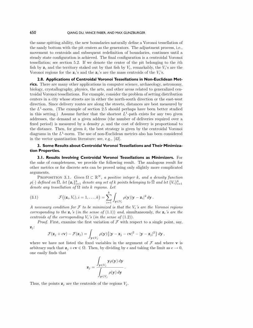
650 QIANG DU, VANCE FABER, AND MAX GUNZBURGER
the same spitting ability, the new boundaries naturally define a Voronoi tessellation ofthe sandy bottom with the pit centers as the generators. The adjustment process, i.e.,movement to centroids and subsequent redefinition of boundaries, continues until asteady state configuration is achieved. The final configuration is a centroidal Voronoitessellation; see section 5.2. If we denote the center of the pit belonging to the ithfish by zi and the territory staked out by that fish by Vi, remarkably, the Vi’s are theVoronoi regions for the zi’s and the zi’s are the mass centroids of the Vi’s.
2.8. Applications of Centroidal Voronoi Tessellations in Non-Euclidean Met-rics. There are many other applications in computer science, archaeology, astronomy,biology, crystallography, physics, the arts, and other areas related to generalized cen-troidal Voronoi tessellations. For example, consider the problem of setting distributioncenters in a city whose streets are in either the north-south direction or the east-westdirection. Since delivery routes are along the streets, distances are best measured bythe L1-norm. (The example of section 2.5 should perhaps have been better studiedin this setting.) Assume further that the shortest L1-path exists for any two givenaddresses, the demand at a given address (the number of deliveries required over afixed period) is measured by a density ρ, and the cost of delivery is proportional tothe distance. Then, for given k, the best strategy is given by the centroidal Voronoidiagrams in the L1-norm. The use of non-Euclidean metrics also has been consideredin the vector quantization literature; see, e.g., [42].
3. Some Results about Centroidal Voronoi Tessellations and Their Minimiza-tion Properties.
3.1. Results Involving Centroidal Voronoi Tessellations as Minimizers. Forthe sake of completeness, we provide the following result. The analogous result forother metrics or for discrete sets can be proved using only slightly more complicatedarguments.Proposition 3.1. Given Ω ⊂ R
N , a positive integer k, and a density functionρ(·) defined on Ω, let ziki=1 denote any set of k points belonging to Ω and let Viki=1denote any tessellation of Ω into k regions. Let
F((zi, Vi), i = 1, . . . , k) = k∑i=1
∫y∈Vi
ρ(y)|y − zi|2 dy .(3.1)
A necessary condition for F to be minimized is that the Vi’s are the Voronoi regionscorresponding to the zi’s (in the sense of (1.1)) and, simultaneously, the zi’s are thecentroids of the corresponding Vi’s (in the sense of (1.2)).
Proof. First, examine the first variation of F with respect to a single point, say,zj :
F(zj + εv)−F(zj) =∫
y∈Vjρ(y)
|y − zj − εv|2 − |y − zj |2dy ,
where we have not listed the fixed variables in the argument of F and where v isarbitrary such that zj+εv ∈ Ω. Then, by dividing by ε and taking the limit as ε→ 0,one easily finds that
zj =
∫y∈Vj
yρ(y) dy∫y∈Vj
ρ(y) dy.
Thus, the points zj are the centroids of the regions Vj .

CENTROIDAL VORONOI TESSELLATIONS 651
Next, let us hold the points ziki=1 fixed and see what happens if we choose atessellation Viki=1 other than the Voronoi tessellation Vjkj=1. Let us compare thevalue of F((zi, Vi), i = 1, . . . , k) given by (3.1) with that of
F((zj , Vj), j = 1, . . . , k
)=
k∑j=1
∫y∈Vj
ρ(y)|y − zj |2 .(3.2)
At a particular value of y,
ρ(y)|y − zj |2 ≤ ρ(y)|y − zi|2 .(3.3)
This result follows because y belongs to the Voronoi region Vj corresponding to zjand possibly not to the Voronoi region corresponding to zi; i.e., y ∈ Vi but Vi is notnecessarily the Voronoi region corresponding to zi. Since Viki=1 is not a Voronoitessellation of Ω, (3.3) must hold with strict inequality over some measurable set ofΩ. Thus,
F((zj , Vj), j = 1, . . . , k) < F((zi, Vi), i = 1, . . . , k)so that F is minimized when the subsets Vi, i = 1, . . . , k, are chosen to be the Voronoiregions associated with the points zi, i = 1, . . . , k.
Another interesting and useful point follows from the above proof. Define thefunctional
K((zi), i = 1, . . . , k) =k∑i=1
∫y∈Vi
ρ(y)|y − zi|2 dy ,(3.4)
where Vi’s are the Voronoi regions corresponding to the zi’s. Note that the functionalin (3.4) is only a function of the zi’s since, once these are fixed, the Vi’s are determined;for the functional in (3.1) it is assumed that the zi’s and Vi’s are independent. Forminimizers of the functionals in (3.1) and (3.4), we have the following result.Proposition 3.2. Given Ω ⊂ R
N , a positive integer k, and a density functionρ(·) defined on Ω, then F and K have the same minimizer.
3.2. Existence of a Minimizer. Given Ω ⊂ RN , a positive integer k, and a densityfunction ρ(·) defined on Ω, let ziki=1 denote any set of k points belonging to Ω and letViki=1 denote any tessellation of Ω into k regions. LetK = Z = (z1, z2, . . . , zk), zj ∈Ω. Let Ai = |Vi|, the area of Vi, and A = (A1, . . . , Ak). Then, one easily obtainsthe following results.Lemma 3.3. A is continuous [47].Lemma 3.4. K is continuous and thus it possesses a global minimum.Proof. Let Z,Z′ ∈ K. Then,
|K(Z)−K(Z′)| =∣∣∣∣ k∑i=1
(∫y∈Vi
−∫
y∈V ′i
)ρ(y)|y − zi|2 dy
+∫
y∈V ′iρ(y)
(|y − zi|2 − |y − z′i|2)dy∣∣∣∣ .
If Ω is compact and ρ is continuous, then there exists a constant C such that
|K(Z)−K(Z′)| ≤ Ck∑i=1
|Ai −A′i|+ |zi − z′i|.

652 QIANG DU, VANCE FABER, AND MAX GUNZBURGER
Then, the continuity of K follows from Lemma 3.3. The existence of the globalminimizer then follows from the compactness of K.
In general, K may also have some local minimizers; we now show that a localminimizer of K will give nondegenerate Voronoi diagrams.Proposition 3.5. Assume that ρ(y) is positive except on a set of measure zero
in Ω. Then, local minimizers satisfy zi = zj for i = j.Proof. Suppose that this is not the case. Without loss of generality, denote a
local minimizer by zimi=1 with 1 ≤ m < k. Define
W(z1, . . . , zm) =m∑i=1
∫y∈Vi
ρ(y)|y − zi|2 dy .
For any small δ > 0, pick zm+1 = zj , j = 1, . . . ,m, with minj |zm+1 − zj | ≤ δ anddefine Vim+1
1 to be the Voronoi regions corresponding to z1, z2, . . . , zm+1. Let
W(z1, . . . , zm+1) =m+1∑i=1
∫y∈Vi
ρ(y)|y − zi|2 dy .
Let f(y) = ρ(y)|y − zi|2 for any y ∈ Vi, i = 1, . . . ,m, and f(y) = ρ(y)|y − zi|2 forany y ∈ Vi, i = 1, . . . ,m+ 1. Then,
W(z1, . . . , zm) =∫
Ωf(y)dy and W(z1, . . . , zm+1) =
∫Ωf(y)dy .
Note that
f(y) = f(y) for any y ∈ Vi ∩ Vi, i = 1, . . . ,m;f(y) ≥ f(y) for any y ∈ Vi \ Vi, i = 1, . . . ,m;f(y) > f(y) for any y ∈ Vm+1.
Since the set Vm+1 has positive measure, W(z1, . . . , zm+1) <W(z1, . . . , zm), which isa contradiction.
Remark 3.6. For the general metric (assuming that ρ vanishes only on a setof zero measure), existence is provided by the compactness of the Voronoi regions.Uniqueness is also attained if the Voronoi regions are convex and if for any y1,y2 ∈ Vi,y1 = y2, the inequality
d(z, λy1 + (1− λ)y2) < λd(z,y1) + (1− λ)d(z,y2)
is valid for some λ ∈ (0, 1) on a subset of Vi with positive measure.3.3. Results for the Discrete Case. There are many results available, especially
in the statistics literature, for centroidal Voronoi tessellations in the discrete casedescribed in section 1.1, for which the given set to be tessellated is finite-dimensional,e.g., W = yimi=1, a set of m points in RN . The energy (which is also often referredto as the variance, cost, distortion error, or mean square error) is now given by
F((zi, Vi), i = 1, . . . , k) = k∑i=1
∑y∈Vi
ρ(y)|y − zi|2 dy,(3.5)
where Viki=1 is a tessellation ofW and ziki=1 are k points belonging toW or, moregenerally, to RN .
CENTROIDAL VORONOI TESSELLATIONS 653
Many results involve properties of centroidal Voronoi tessellations as the numberof sample points becomes large, i.e., as m → ∞. The convergence of the energy wasshown in [40]. The convergence of the centroids, i.e., the cluster centers, was proved in[52] for the Euclidean metric under certain uniqueness assumptions. The asymptoticdistribution of cluster centers was considered in [53], where it was shown that thecluster centers, suitably normalized, have an asymptotic normal distribution. Theseresults generalize those of [20]. Generalization to separable metric spaces was givenin [50].
In [63], some large-sample properties of the k-means clusters (as the number ofclusters k approaches ∞ with the total sample size) are obtained. In one dimension,it is established that the sample k-means clusters are such that the within-clustersums of squares are asymptotically equal, and that the sizes of the cluster intervalsare inversely proportional to the one-third power of the underlying density at themidpoints of the intervals. The difficulty involved in generalizing the results to themultivariate case is mentioned.
In vector quantization analysis [17], clustering k-means techniques have also beenused and analyzed. A vector quantizer is a mapping Q of N -dimensional Euclideanspace RN into itself such that Q has a finite range space of, say, k vectors. Given adistortion measure d(X,Q(X)) between an input vectorX and the quantized represen-tation Q(X), the goal is to find the mapping Q that minimizes the average distortionwith respect to the probability distribution F governing X, D(Q,F ) = Ed(X,Q(X)).The mathematical formulation of the average distortion is similar to that of the energyfunctional given in (3.1) for the continuous case and (3.5) for the discrete case. In[1], several convergence and continuity properties for sequences of vector quantizersor block source codes with a fidelity criterion are developed. Conditions under whichconvergence of a sequence of quantizers Qn and distributions Fn implies convergenceof the resulting distortion D(Qn, Fn) as n → ∞ are also provided. These resultsare in turn used to draw conclusions about the existence and convergence of optimalquantizers.
The results are intuitive and useful for studying convergence properties of designalgorithms used for vector quantizers. Note that there do not yet exist general algo-rithms capable of finding optimal quantizers (except when the distribution has finitesupport and all quantizers can be exhaustively searched). Most algorithms can findonly locally optimal quantizers, and hence convergence results for optimal quantizersare currently of limited application.
Another interesting aspect of the discrete problem involves the reduction of thespatial dimension. For many practical problems, it is desirable to visualize the re-sulting centroidal Voronoi diagrams or the optimal clusters by some means. Varioustechniques, such as the projection pursuit method [11, 18, 29, 58], have been studiedin the statistics literature. They can be used to characterize the centroidal Voronoidiagrams via lower dimensional approximations.
3.4. Connections between the Discrete and Continuous Problems. The dis-crete problem is obviously connected to the continuous problem outlined earlier. Thiswas pointed out in [30], where it was shown that the k-clustering problem can beviewed as a discrete version of the continuous geographical optimization problemstudied in [33]; the latter is equivalent to minimizing the function in (3.1). Theauthors point out that further investigations are deserved.
For nonuniformly distributed points, an alternative formulation of the discretek-clustering problem might reveal even closer ties with the continuous problem. For
654 QIANG DU, VANCE FABER, AND MAX GUNZBURGER
example, consider the set of m points W = ymj=1 in RN along with a clustering
of these points into k clusters Wiki=1 and associated cluster centers xiki=1 givenby (2.4). Next, consider the Voronoi diagram Viki=1 in R
N generated by the pointsxiki=1, with suitable truncation of the possible unbounded regions so that eachVoronoi region remains bounded, i.e., ignoring the overload, as is done in vectorquantization [17]. We may associate with each point xi a weight ρj = 1/|Vj | (|Vi|being the area of the corresponding Voronoi region). Then, if W contains a largenumber of points, i.e., if m is large, and the areas of Vi’s become small, we get from(2.5) that
V ar(W ) =k∑i=1
∑yj∈Wi
|yj − xi|2 =k∑i=1
∑yj∈Wi
ρj |yj − xi|2|Vj |
≈k∑i=1
∫W∗i
ρ(x)|x − x∗i |2 dx = F((x∗i ,W ∗i ), i = 1, . . . , k),with W ∗i forming a Voronoi tessellation of a suitable domain containing W andx∗i being the mass centroids of W
∗i . F is as given in (3.1). ρ is a suitable density
distribution, reflecting how the points in W are distributed in space. In this context,one can see that the connection made in [24, 30] is valid only if the points in W aremore or less uniformly distributed. Indeed, to get uniform density in the continuousproblem, we may define the weighted mean of cluster Wi as
xi =
∑xj∈Wi
ρ−1j xj∑
xj∈Wiρ−1j
and the generalized variances as
V ar(Wi) =∑
xj∈Wi
ρ−1j |xj − xi|2 , V ar(W ) =
k∑i=1
V ar(Wi) .
With the modification, we get, when the Vi’s are small, that
V ar(W ) =k∑i=1
∑xj∈Wi
ρ−1j |xj − xi|2 ≈
k∑i=1
∫W∗i
|x − x∗i |2dx .
With the new formulation, one can perhaps study how to generalize the stochastic 2-clustering or k-clustering algorithms presented in section 4.2. It is possible that newalgorithms may be constructed for which good estimates can be obtained in caseswhere the balancing conditions given in [24, 30] are not met. It may also lead to abetter sampling strategy and improvements in performance.
4. Probabilistic Approaches to Determining Centroidal Voronoi Tessellations.In this section, we discuss probabilistic approaches for the determination of centroidalVoronoi tessellations of a given set.
4.1. A Sequential, Random Sampling Algorithm. We begin with an elegantrandom sequential sampling method which has the advantage that it does not requirethe calculation of Voronoi sets. (It is referred to as the random k-means method, orsimply the k-means method, since it gives a partition of a sample into k sets by takingmeans of sampling points.)
The random k-means method is defined as follows. Given a set Ω, a positiveinteger k, and a probability density function ρ defined on Ω,

CENTROIDAL VORONOI TESSELLATIONS 655
0. select an initial set of k points ziki=1, e.g., by using a Monte Carlo method;set ji = 1 for i = 1, . . . , k;
1. select a y ∈ Ω at random, according to the probability density function ρ(y);2. find the zi that is closest to y; denote the index of that zi by i∗;3. set
zi∗ ←ji∗zi∗ + yji∗ + 1
and ji∗ ← ji∗ + 1 ;
this new zi∗ , along with the unchanged zi, i = i∗, forms the new set of pointsziki=1.
4. If this new set of points meets some convergence criterion, terminate; otherwise,go back to step 1.
Note that (ji − 1) equals the number of times that the point zi has been updated.The random k-means algorithm has the following interpretation. At the th stage
of the algorithm, one starts with the positions of the cluster centers, i.e., the means,zi, i = 1, . . . , k, and a clustering of (+ k − 1) points (the original k points of step 0plus the (− 1) points y previously selected in step 1) into k corresponding clusters.One then selects a new random point y, locates the closest cluster center, and addsthis to the corresponding cluster. Of course, one also updates the mean, i.e., thecluster center, of the enlarged cluster.
The random k-means method has been analyzed in [40], where the almost sureconvergence of the energy is proved. The mass centers often are also referred toas cluster centers, which are simply the means of the Voronoi regions. Employingthe Euclidean metric, for various general optimization problems that correspond tof(s) = sr in (1.10), the mean could be replaced by the median, the mode, or themidrange for r = 1, r → 0, and r → ∞, respectively. In [40], various examples arediscussed for which the k-means methods fail to give the optimal centroidal Voronoiregions. Generalizations to non-Euclidean metrics were also presented there. Thekey is to measure the closeness in the sense of the metric and replace the mean instep 3 by using the more general definition of the mass center. A proof of the weakconvergence of the energy functional was also given in [40].
Extensions to separable metric spaces are given in [51]. Let P be a probabilitymeasure on the separable metric space (T, d). Define the energy functional (clusteringcriterion) by
W (A,P ) =∫
min1≤i≤k
φ(d(x, ai))P (dx) ,
where A = a1, . . . , ak ⊂ T is the set of mass centers (cluster means) and φ is anondecreasing function satisfying certain conditions. Define Wk(P ) = infW (A,P ):|A| = k, and let A∗k(P ) be the class of all minimizing sets A∗ = a∗1, . . . , a∗k. Thealmost sure convergence Wk(Pn)→Wk(P ) as Pn converges to P weakly is proved in[51].
Variations of the k-means methods are proposed in [35] using bootstrapping tech-niques. Advantages of the bootstrap methods are discussed and the performance ofbootstrap confidence sets is compared with that of the Monte Carlo confidence setsdiscussed in [52].
In the discrete, finite-dimensional case (see section 1.1) for which one is given,instead of Ω, a set of points W = ym=1 belonging to R
N , a deterministic variant ofthe k-means algorithm is easily defined by choosing the points y not at random, butsequentially through the setW . In section 5.1, we will return to the finite-dimensional
656 QIANG DU, VANCE FABER, AND MAX GUNZBURGER
version of the algorithm. Some deterministic and stochastic variants of the k-meansalgorithm in the discrete case are given in [4].
4.2. A Random 2-Clustering Algorithm for the Discrete Case. For variance-based k-clustering analysis of a finite-dimensional set of pointsW = yM=1 belongingto RN , another type of probabilistic algorithm, which we refer to as the m-samplealgorithm, has been studied in [24, 30, 31, 32]. The 2-clustering version is given asfollows:
0. Sample an initial subset T of m points from W , e.g., by using a Monte Carlomethod.
1. For every linearly separable 2-clustering (T1, T2) of T ,• compute the centroids t1 and t2 of T1 and T2, respectively;• find a 2-clustering (W1,W2) of W divided by the perpendicular bisector ofthe line segment connecting t1 and t2;
• compute the total variance of the 2-clustering (W1,W2) and maintain theminimum among these values.
2. Output the 2-clustering of W with minimum value above.Note that the preceding algorithm can be generalized to the k-clustering cases. Itwas pointed out that the random m-sample algorithm can be used to find good initialclusters for the deterministic algorithms discussed in section 5.1. Under suitable bal-ancing conditions on the optimal 2-clusters, it was shown in [30, 31] that in O(mNM)time, the m-sample algorithm finds a 2-cluster whose variance is within a factor of1 +O(1/(δm)) of the optimal value with probability 1− δ for small δ.
In the general application of k-clustering, it was proposed [32] that the m-samplealgorithm may be applied in a top-down recursive manner and that the heap is used toobtain the subset with the maximum variance to be divided in the subsequent step.Extensive numerical tests were performed in [32] along with comparisons to othermethods such as those used in [25, 62]. Suggestions on directly sampling k-clusters,without using the top-down binary partition technique, are also proposed.
5. Deterministic Approaches to Determining Centroidal Voronoi Tessella-tions. In this section, we discuss some deterministic approaches for the determinationof centroidal Voronoi tessellations of a given set. We refer to [47] for a discussion andreferences on algorithms to compute arbitrary Voronoi diagrams.
5.1. Sequential Sampling Algorithms for the Discrete Case. We return to thedeterministic version of the k-means algorithm of section 4.1, which can be used in thediscrete case; see [19]. Given a discrete, finite-dimensional set of points W = ym=1belonging to RN , an integer k > 1, and an initial set of cluster centers ziki=1, thenfor each y ∈W ,
1. find the zi that is closest to y; denote the index of that zi by i∗;2. assign y to the cluster corresponding to zi∗ ;3. recompute the cluster center zi∗ to be the mean of the points belonging to the
corresponding cluster.An efficient implementation of this algorithm for large data sets is given in [21]; seealso [10]. It is shown in [55] that, for the quadratic metric, the energy converges to alocal minimum value.
Other deterministic algorithms for determining the cluster centers are given in [25,62, 64]. These involve recursive clustering into hyperboxes having faces perpendicularto the coordinate axes.

CENTROIDAL VORONOI TESSELLATIONS 657
If m is finite, then obviously the clustering problem can be solved in a finitenumber of steps. In fact, the following result is given in [30, 32].Theorem 5.1. For quadratic energies, the clustering problem for m points in
RN into k clusters can be solved in O(mkN+1) steps.This bound is very pessimistic for large k. However, it is also known that, in
general, the problem of finding the optimal clustering is an NP-hard problem [12, 13,48]. Other results on the k-means method and its relation to the optimality conditionsof a related mathematical programming problem can be found in [55].
5.2. Lloyd’s Method. Next, we discuss a method that is an obvious iterationbetween constructing Voronoi tessellations and centroids. Given a set Ω, a positiveinteger k, and a probability density function ρ defined on Ω,
0. select an initial set of k points ziki=1, e.g., by using a Monte Carlo method;1. construct the Voronoi tessellation Viki=1 of Ω associated with the points ziki=1;2. compute the mass centroids of the Voronoi regions Viki=1 found in step 1;
these centroids are the new set of points ziki=1.3. If this new set of points meets some convergence criterion, terminate; otherwise,
return to step 1.(Here we will not discuss termination procedures since they are very much dependenton the specific application.) This method, at least in the electrical engineering litera-ture, is known as Lloyd’s method [39]. (A second method was also proposed by Lloydfor one-dimensional problems; it is similar to a shooting approach, i.e., one guessesthe leftmost mass center, then determines the end-point of the leftmost region, thenextrapolates to get the next leftmost center, etc. No generalization to higher spacedimensions is known.)
Lloyd’s method may be viewed as a fixed point iteration. For example, considerthe case of Ω ⊂ R
N , i.e., of (1.1)–(1.3). Let the mappings Ti : RkN → RN , i =
1, . . . , k, be defined by
Ti(Z) =
∫Vi(Z)
yρ(y) dy∫Vi(Z)
ρ(y) dy,
where
Z = (z1, z2, . . . , zk)T and Vi(Z) = Voronoi region for zi, i = 1, . . . , k .
Let the mapping T : RkN → RkN be defined by
T = (T1,T2, . . . ,Tk)T .
Clearly, centroidal Voronoi tessellations are fixed points of T(Z).
5.3. Variations on Lloyd’s Method. In [38] (see also [15]), a probabilistic varia-tion of Lloyd’s method is proposed. The method is essentially a continuation methodfor the global optimization problem in the spirit of simulated annealing. The data,i.e., the density function, are corrupted (perturbed) by noise. For strong noise, thecentroidal region essentially depends only on the noise; it is assumed that a uniquelocal minimum exists. Then, the noise level is slightly reduced in subsequent stepsand the local minima from previous steps are used as initial guesses for later steps. Itwas argued that the algorithm might converge although new local minima might havebeen introduced. The algorithm stops when the noise level is reduced to zero. No

658 QIANG DU, VANCE FABER, AND MAX GUNZBURGER
convergence theory was provided, but further studies of such ideas were given in [1].There, it is claimed that their analysis implies that globally optimal quantizers canbe designed by adding “nice” noise to the original distribution and then slowly reduc-ing the noise to zero under the requirement that “close” distributions yield “close”optimal quantizers. These properties, however, have not been shown to be valid in allcases.
Another generalization, in the form of a two-stage algorithm, is studied in [61].For that algorithm, the first stage of Lloyd’s iteration is applied so as to reduce thevalue of error functionals such as
k∑i=1
∫Vi
ρ(y)f(d(y, zi)) dy
and its discrete analogs. At the second stage, a search for a minimizer is performed,using a hybrid of a dynamic programming algorithm and a Lloyd-type algorithmthat achieves the absolute optimality of dynamic programming with much less com-putational effort. For a continuous distribution with log-concave density ρ and anincreasing convex weighting function f , a reliable method is presented for comput-ing the optimal parameters with a known precision, using a generalization of Lloyd’smethod.
In image-data compression applications, region-based algorithms have also beenstudied in [8]. Voronoi diagram–based vector quantization techniques are used in high-frequency regions or in regions with uncorrelated data; polynomial approximations areused in smooth regions or in regions with highly correlated data.
A number of other generalizations are discussed in [15, 43].
5.4. Descent or Gradient Methods. One can construct general iterative pro-cedures for determining the centroidal Voronoi tessellations by following a descentsearch algorithm of the type
Z(n+1) = Z(n) − αn∂C∂z(Z(n)) , n = 1, 2, . . . ,(5.1)
where the scalar αn is a suitable chosen step size. Here, one can choose C(Z) to be afunction whose stationary points are fixed points of the Lloyd map T(Z). See section6.2 for a further discussion.
For the discrete case, gradient methods, including steepest descent methods withline searches, are considered in [33]. The relation between centroidal Voronoi tes-sellations, e.g., optimal clustering, and stationary points of associated functions isdiscussed in [55].
5.5. Newton-Like Methods. One may naturally compute the fixed point of Tusing Newton’s method, i.e.,(
I − ∂T∂z(Z(n))
)(Z(n+1) − Z(n)) = −Z(n) +T(Z(n)) , n = 1, 2, . . . .
For smooth density functions, one may easily verify that the Newton iteration islocally convergent at a quadratic rate whenever the initial guess is close enough tothe fixed point. In practice, however, calculations of ∂T/∂z can be expensive inspace dimensions higher than one or if the density function is not smooth. Thus, aquasi-Newton method may offer a better alternative.
CENTROIDAL VORONOI TESSELLATIONS 659
6. Some Results Concerning Lloyd’s Method. Lloyd’s method as given in sec-tion 5.2, or under other names, has been proposed and studied by many authors ina number of different applications contexts. In this section, we discuss some of theproperties associated with Lloyd’s method.
6.1. Derivatives of the Energy and the Lloyd Map. Let U = ujMj=1 ∈ RMN
be the vertices of the Voronoi regions generated by Z = zik1 ∈ RkN . Geometricalconsideration tells us that each uj is the circumcenter of the Delaunay simplex formedby some zi’s whose Voronoi regions share common faces. Clearly, the map: Z → Uis linear; we denote it by G(Z). Also, it is useful to know that if uj and ujll≥1 arethe vertices of the common face ∆nm between two adjacent Voronoi regions generatedby zm and zn, then we have(
λ0uj +∑l≥1
λlujl − (zm + zn))· (zm − zn) = 0(6.1)
for any set of nonnegative parameters λll≥0 with∑l≥0 λl = 1 such that λ0uj +∑
l≥1 λlujl ∈ ∆nm. This is simply the perpendicular bisector property of Voronoidiagrams; i.e., the face ∆nm bisects the line segment joining zm and zn and that linesegment is perpendicular to the face.
Next, we let Vi(U) denote the set of Voronoi regions having U as vertices andlet M be a diagonal matrix with entries
Mi =∫Vi(U)
ρ(y) dy ∀ i .
Let F denote the map that maps vertices U to the mass centroids of Vi(U), i.e.,
F : U →
1Mi
∫Vi(U)
ρ(y)y dy ∀ i.
Clearly, we see that the Lloyd map T is given by T = F G. We shall use thefollowing notation for the derivative maps:
F =dFdu
and G′ =dGdz.
We now investigate the relations between the maps F and G and the derivativemaps of the energy F (see (3.1)), which are recast as
H(Z,U) =k∑i=1
∫Vi(U)
ρ(y)|y − zi|2 dy .
In addition, in light of Propositions 3.1 and 3.2, we also define
G(Z) = H(Z,G(Z)) .Now, it is simple to see that
∂H∂zi
= 2zi∫Vi(U)
ρ(y)dy − 2∫Vi(U)
ρ(y)ydy
so that∂H∂Z
= 2M(U)(Z − F(U)) .(6.2)

660 QIANG DU, VANCE FABER, AND MAX GUNZBURGER
Furthermore, we have
∂2H∂Z2 = 2M(U) .
In order to differentiate with respect to u, we first state a result concerningdifferentiations with respect to change in domain.Lemma 6.1. Let Ω = Ω(U) be a region that depends smoothly on U and that has
a well-defined boundary. If F =∫
Ω(U) f(y)dy, then
dF
dU=∫∂Ω(U)
f(y)y · n dy ,
where n is the unit outward normal and y denotes the derivative of the boundarypoints with respect to changes in U.
Since U = G(Z), we have that ρ(y)|y− zj |2 = ρ(y)|y− zn|2 for any y belongingto ∆nm, where ∆
nm again denotes the common face of the Voronoi regions generated
by zm and zn. Then, by Lemma 6.1, we have that∂H∂U
∣∣∣U=G(Z)
= 0 .
In fact, for U close to G(Z), in the sense that the regions formed by G(Z) aresimple perturbations of that of U with the same topological structure, using theorthogonal bisector property (6.1), we can show that
∂H∂U
= A(U,Z)(U − G(Z)) .
The matrix A, or more precisely its action, is defined as follows. Let the verticesof the common face ∆nm between Vm and Vn be denoted by uj and ujll≥1 andlet y = λ0uj +
∑l≥1 λlujl ∈ ∆nm for parameters λll≥0 belonging to the standard
simplex ∆ = λl ≥ 0 ∀ l, ∑l λl ≤ 1. Then, the matrix A is defined by
(A(U,Z)(U − G(Z)))i = 2∑
uj∈∆nm
∫∆nm
λ0nnm ρ(λ0uj +
∑l≥1
λlujl
)(zm − zn)
·(λ0
(uj − Gj(Z)
)+∑l≥1
λl
(ujl − Gjl(Z)
))dλλλ ,
where nnm is the unit normal of ∆nm that has positive angle with zn − zm. Thus, wehave the following result.Proposition 6.2. The derivative of G is given by
∂G∂Z(Z) = 2M(G(Z))(Z − T(Z)) .(6.3)
Thus, if the density function ρ is positive except on a set of measure zero, the station-ary points of G are given by fixed points of the Lloyd map T(Z).
In componentwise form, (6.3) is equivalent to
∂G∂zi
(Z) = 2zi∫Vi
ρ(y)dy − 2∫Vi
ρ(y)ydy .
Furthermore,
∂2G∂z2 (Z) = 2M(G(Z))(I − F(G(Z))G′(Z))
+2(G′(Z))T (M(G(Z)))T (Z − T(Z)) .

CENTROIDAL VORONOI TESSELLATIONS 661
Fig. 6.1 Two possible moves from the saddle point of the Voronoi tessellations of a square. The leftmove increases the energy while the right move decreases the energy.
Thus, we arrive at the following result.Proposition 6.3. At the stationary point, i.e., whenever Z = T(Z), we have
∂2G∂Z2 (Z) = 2M(G(Z))
(I − ∂T
∂z(Z)).
We see that the local convexity of the energy is related to the Jacobian of theLloyd map, which in turn affects the local convergence properties of the Lloyd fixedpoint iteration.
In fact, if the energy is locally strictly convex at the minimum, then
M(G(Z))(I − ∂T
∂z(Z))
is positive definite.
So, the eigenvalues of
M1/2(I − ∂T
∂z(Z))M−1/2 = I −M1/2 ∂T
∂z(Z)M−1/2
are all positive, which implies that
the eigenvalues of∂T∂z(Z) are real and less than 1,
a necessary condition for T to be a local contraction.On the other hand, a fixed point of the Lloyd map does not necessarily correspond
to a local minimum of the energy. Take the example of two points and the square[−1, 1]2 given in Figure 1.2. One can show that the partition along the midlinecorresponds to a local minimum but the one along the diagonal corresponds to asaddle point. In fact, the energy decreases as the diagonal rotates toward the middlevertical line. (We can treat rotation to the middle horizontal line in a similar manner.)The mass centers move along the points (∓1/2± ε2/6,±1/3ε), where 1/ε is the slope;ε = 1 corresponds to the diagonal and ε = 0 corresponds to the vertical midline. Theenergy is given by 5/12 + ε2/18 − ε4/36, which decreases as ε goes from 1 to 0. Onthe other hand, if we translate the diagonal parallel to itself, i.e., if we move the twopoints along the other diagonal so that one center of mass is closer to the center ofthe square than the other, then the energy increases. Thus, the diagonal partitionforms a saddle point for the energy; see Figure 6.1.
6.2. General Descent Methods and Lloyd’s Method. With the gradient of theenergy given by (6.3), Lloyd’s method can be viewed as a special case of a generalgradient method. One can construct general iterative procedures for determining the

662 QIANG DU, VANCE FABER, AND MAX GUNZBURGER
centroidal Voronoi regions, i.e., for minimizing the energy, by following a descentsearch algorithm of the form
Z(n+1) = Z(n) − αnB(n) ∂G∂z(Z(n)) , n = 1, 2, . . . ,(6.4)
where the matrix B(n) is positive definite and the scalar αn represents the step size.It is easy to see that if αn is small enough, then G(Z(n+1)) < G(Z(n)) unless we havereached a stationary point. Lloyd’s method is simply the special case of (6.4) withαn = 1/2 and B(n) =M(G(Z(n)))−1.
6.3. Convergence of Lloyd’s Method for a Class of One-Dimensional Prob-lems. Lloyd’s method has been shown to be convergent locally for a class of one-dimensional problems; see, e.g., [36]. Here, we present a simple proof for a result ofthis type. Without loss of generality, we assume that Ω = [0, 1]. Let the densityfunction ρ be smooth and strictly positive. In addition, ρ is assumed to be strictlylogarithmically concave; i.e., log ρ is a strictly concave function. This is equivalent to
(log ρ)′′ < 0 or − ρ′
ρstrictly increasing.
Given k points x = xi, i = 1, . . . , k such that 0 ≤ x1 < x2 < · · · < xk−1 <xk ≤ 1, it is clear that the corresponding Voronoi regions are the intervals V1 =[0, x1+x2
2 ], Vi = [xi+xi−12 , xi+xi+1
2 ] for i = 2, . . . , k − 1, and Vk = [xk−1+xk2 , 1]. Let
Mi =∫Viρ(y)dy. The Lloyd map is then defined as
Ti(x) =1Mi
∫Vi
yρ(y) dy .
At the fixed point x = T(x), the Jacobian matrix is a tridiagonal matrix with
∂Ti∂xi−1
=(xi − xi−1)
4Miρ
(xi + xi−1
2
),
∂Ti∂xi+1
=(xi+1 − xi)
4Miρ
(xi + xi+1
2
),
∂Ti∂xi
=∂Ti∂xi−1
+∂Ti∂xi+1
.
One easily sees that ∂T/∂x at the fixed point is a nonnegative matrix. Next, weconsider
M2i
1−∑j
∂Ti∂xj
=M2i − 2M2
i
∂Ti∂xi−1
− 2M2i
∂Ti∂xi+1
.

CENTROIDAL VORONOI TESSELLATIONS 663
Let Vi = [y−, y+] and note that xi = Ti(x); then,
M2i − 2M2
i
∂Ti∂xi−1
− 2M2i
∂Ti∂xi+1
=[∫
Vi
ρ(y)dy]2
− ρ(y−)[∫
Vi
(ρ(y)y − ρ(y)y−
)dy
]−ρ(y+)
[∫Vi
(ρ(y)y+ − ρ(y)y
)dy
]=∫Vi
∫Vi
ρ(s)ρ(t)dsdt−∫Vi
ρ(t)[∫
Vi
(ρ′(s)(s− t) + ρ(s)
)ds
]dt
=∫Vi
∫Vi
ρ′(s)ρ(t)(t− s)dsdt
=12
∫Vi
∫Vi
(ρ′(s)ρ(t)− ρ′(t)ρ(s)
)(t− s)dsdt
=12
∫Vi
∫Vi
ρ(t)ρ(s)(ρ′(s)ρ(s)
− ρ′(t)ρ(t)
)(t− s)dsdt
> 0 ,
where the last step follows from the logarithmic concavity. Thus, by the Gerschgorintheorem, the spectral radius of the Jacobian is less than 1 and we have the localconvergence of the Lloyd iteration.Proposition 6.4. Assume that ρ(x) is a smooth density function that is strictly
positive and strictly logarithmically concave on Ω. Then, the Lloyd map T is a localcontraction map near its fixed points. Consequently, the Lloyd iteration is locallyconvergent.
From the proof, we see that the essential requirement on the density function isto have (
ρ′(s)ρ(t)− ρ′(t)ρ(s))(t− s) > 0
for any (t, s) except for a set of measure zero.As a consequence of Propositions 6.3 and 6.4, we also have the local convexity of
the energy.Proposition 6.5. Under the assumptions on ρ of Proposition 6.4, the energy
functional G is locally strictly convex near any stationary point.
6.4. Other Results in One Dimension.
6.4.1. Equal Partition of Energy. We consider the unit interval with constantdensity ρ(x) = 1. Then, for given k, the optimal centroids with k intervals are givenby xi = (2i− 1)/2k, i = 1, . . . , k. A simple calculation shows that∫
Vi
|x− xi|2dx =1
12k3 ∀ i ,
i.e., the energy is equally partitioned over the k Voronoi regions. One naturally askswhether the centroidal Voronoi diagram for general densities shares the equal partitionof energy property. The answer is negative in general. For example, let the densityfunction be given by ρ(x) = x and k = 2. Then the two centroidal Voronoi regions

664 QIANG DU, VANCE FABER, AND MAX GUNZBURGER
are given by (0, z) and (z, 1), where z = (√5 − 1)/2, and the centers of mass are
given by 2z/3 and 4z/3, respectively. The values of energy on each region are givenby (7− 3
√5)/72 and (83− 37
√5)/72.
An interesting question is related to the distribution of the energy (also referred toas the cost or variance or distortion error, etc., in some contexts) when the number ofgenerators gets large. Let hi = |Vi|. Under the condition that the density is boundedand strictly positive, we have h = maxhi → 0 as k, the number of generators, goesto infinity. Then, from ∫
Vi
ρ(x)(x− xi)dx = 0 ∀ i ,
we get the asymptotic form of the energy in each region as∫Vi
ρ(x)(x− xi)2dx =∫Vi
ρ(x)(x− xi)(x−mi)dx
≈ 112[ρ(mi) + ρ′(mi)(mi − xi)]h3
i +O(h5i ) ∀ i ,
where mi is the midpoint of the interval Vi. On the other hand, using Taylor expan-sions, we obtain∫
Vi
ρ(x)(x− xi)dx = ρ(mi)(mi − xi)hi +112ρ′(mi)h3
i
+124ρ′′(mi)(mi − xi)h3
i +O(h5i ) ∀ i .
Since mi − xi = (hi+1 − hi)/4, we then obtainhi+1 − hih2i
≈ − ρ′(mi)3ρ(mi)
.
From this, we obtain that the energy in each region is approximately given by
112ρ(mi)h3
i ∀ i .
Furthermore, assuming that the mesh sizes hi are of the form
hi ≈ g(mi)τ ∀ i ,where g is a smoothly varying function and τ is a small parameter, yields that
g(mi+1)− g(mi)τg(mi)2
≈ − ρ′(mi)3ρ(mi)
.
On the other hand,
mi+1 −mi =hi+1 + hi
2= τ
g(mi+1) + g(mi)2
≈ τg(mi),
so that
− ρ′(mi)3ρ(mi)
≈ g(mi+1)− g(mi)τg(mi)2
≈ g(mi+1)− g(mi)mi+1 −mi
1g(mi)
≈ g′(mi)g(mi)
.
CENTROIDAL VORONOI TESSELLATIONS 665
We see that this is satisfied by g(mi) ≈ cρ−1/3(mi) for some constant c, i.e.,
|Vi| ≈cτ
ρ1/3(mi).
Substituting into the asymptotic expression for the energy, we obtain∫Vi
ρ(x)(x− xi)2dx ≈112ρ(mi)h3
i ≈c3τ3
12∀ i .
These two properties are the deterministic analog of the results in [63] for the proba-bilistic k-means clustering that we discussed in the previous section; i.e., under someassumptions on the density function, asymptotically speaking, the energy is equallydistributed in the Voronoi intervals and the sizes of the Voronoi intervals are inverselyproportional to the one-third power of the underlying density at the midpoints of theintervals. In [14], an important conjecture is made which states that asymptotically,for the optimal centroidal Voronoi tessellation, all Voronoi regions are approximatelycongruent to the same basic cell that depends only on the dimension. The basiccell is shown to be the regular hexagon in two dimensions [44], but the conjecture re-mains open for three and higher dimensions. The equidistribution of energy principle,however, can be established based on Gersho’s conjecture [14, 17].
6.4.2. Linear Convergence Rate of Lloyd’s Method. We again consider the unitinterval with constant density ρ(x) = 1 and k points so that the optimal centroidsare given by xi = (2i− 1)/2k, i = 1, . . . , k. Let xn0 = 0 and xnk+1 = 1. Then, Lloyd’smethod is simply given by the iteration xn+1
i = (xni−1+2xni +x
ni+1)/4 for i = 1, . . . , k.
Therefore, the error eni = xni − (2i− 1)/2k satisfies 8en+1 = Tk8en, where
Tk =
1/4 1/4 0 . . . . . . 0 0 01/4 1/2 1/4 · · · · · · 0 0 00 1/4 1/2 · · · · · · 0 0 0· · · · · · · · · · · ·· · · · · · · · · · · ·· · · · · · · · · · · ·0 0 0 · · · · · · 1/2 1/4 00 0 0 · · · · · · 1/4 1/2 1/40 0 0 · · · · · · 0 1/4 1/4
.
Let Tk = Tk + diag(1/4, 0, 0, . . . , 0, 0, 1/4); then, we have that ‖Tk‖ ≤ ‖Tk‖ =cos2 π
2(k+1) and also that ‖Tk‖ ≥ ‖Tk−2‖ = cos2 π2(k−1) so that
sin2 π
2(k + 1)≤ 1− ‖Tk‖ ≤ sin2 π
2(k − 1) .
Thus, for large k,
1− ‖Tk‖ ≈(π2
4k2
).
This shows that Lloyd’s method converges linearly.If, in (5.1), we instead let αn = 1 and B(n) = M(G(Z(n)))−1, then the iteration
matrix becomes 2Tk − I. For large k we have that
1− ‖2Tk − I‖ ≈(π2
2k2
)

666 QIANG DU, VANCE FABER, AND MAX GUNZBURGER
−1 −0.8 −0.6 −0.4 −0.2 0 0.2 0.4 0.6 0.8 1−1
−0.8
−0.6
−0.4
−0.2
0
0.2
0.4
0.6
0.8
1
−1 −0.8 −0.6 −0.4 −0.2 0 0.2 0.4 0.6 0.8 1−1
−0.8
−0.6
−0.4
−0.2
0
0.2
0.4
0.6
0.8
1
−1 −0.8 −0.6 −0.4 −0.2 0 0.2 0.4 0.6 0.8 1−1
−0.8
−0.6
−0.4
−0.2
0
0.2
0.4
0.6
0.8
1
−1 −0.8 −0.6 −0.4 −0.2 0 0.2 0.4 0.6 0.8 1−1
−0.8
−0.6
−0.4
−0.2
0
0.2
0.4
0.6
0.8
1
Fig. 7.1 Two-dimensional Voronoi diagrams for a constant density function in [−1, 1]2; left: MonteCarlo simulation; right: centroidal diagrams; top: 64 generators; bottom: 256 generators.
so that, for large k, the convergence will be twice as fast as that for Lloyd’s method.This situation is similar to overrelaxation. Of course, given the largest and the smallesteigenvalues λmax and λmin of Tk, the optimal parameter α is determined from
1 + α(λmax − 1) = −1− α(λmin − 1) ,
i.e.,
αopt =2
2− λmax − λmin,
which implies a convergence rate on roughly the same order as that for the choiceα = 2.
7. Numerical Experiments. We now illustrate centroidal Voronoi tessellationsof a square; we compare them with Monte Carlo–based Voronoi tessellations and alsoshow the effects of different density functions. For the centroidal Voronoi tessellations,we start from the Voronoi diagrams corresponding to a Monte Carlo distribution ofgenerators and then apply the Lloyd algorithm to find centroidal Voronoi diagrams.

CENTROIDAL VORONOI TESSELLATIONS 667
−1 −0.8 −0.6 −0.4 −0.2 0 0.2 0.4 0.6 0.8 1−1
−0.8
−0.6
−0.4
−0.2
0
0.2
0.4
0.6
0.8
1
−1 −0.8 −0.6 −0.4 −0.2 0 0.2 0.4 0.6 0.8 1−1
−0.8
−0.6
−0.4
−0.2
0
0.2
0.4
0.6
0.8
1
−1 −0.8 −0.6 −0.4 −0.2 0 0.2 0.4 0.6 0.8 1−1
−0.8
−0.6
−0.4
−0.2
0
0.2
0.4
0.6
0.8
1
−1 −0.8 −0.6 −0.4 −0.2 0 0.2 0.4 0.6 0.8 1−1
−0.8
−0.6
−0.4
−0.2
0
0.2
0.4
0.6
0.8
1
−1 −0.8 −0.6 −0.4 −0.2 0 0.2 0.4 0.6 0.8 1−1
−0.8
−0.6
−0.4
−0.2
0
0.2
0.4
0.6
0.8
1
−1 −0.8 −0.6 −0.4 −0.2 0 0.2 0.4 0.6 0.8 1−1
−0.8
−0.6
−0.4
−0.2
0
0.2
0.4
0.6
0.8
1
Fig. 7.2 Perturbation (top center) of a uniform square Voronoi diagram (top left) with 64 generatorsleads to a hexagonal-like lattice (bottom right) with Lloyd’s iteration. The pictures aregenerated at iteration numbers 0, 15, 30, 60, and 120.
In Figure 7.1, results for a constant density function are given. The top two imagesare for 64 generators, the bottom two for 256 generators. For the left pair, the genera-tors of the Voronoi tessellation are distributed randomly with uniform probability; forthe right pair, the generators are those for centroidal Voronoi tessellations. The muchgreater uniformity of the centroidal Voronoi tessellation is obvious. It should be notedthat the working precision of our implementation might affect the final appearancesof the images and prevent them from attaining the diagram with absolute minimumenergy. Of course, for 64 and 256 generators in a square, there exist other obviouscentroidal Voronoi tessellations, e.g., those of 8× 8 and 16× 16, respectively, uniformsquare lattices. (There are many other possible solutions; for example, for 64 gener-ators, we also have arrangements of 64× 1, or 32× 2, or 16× 4 rectangles.) We havethe following comparisons of the values of the energy. For 64 generators, the energyfor the computed centroidal Voronoi diagram of Figure 7.1 is approximately equal to0.0411, while with 256 generators, that energy is approximately equal to 0.0102. Fora centroidal Voronoi diagram with k generators corresponding to a uniform squarelattice, the energy is 8/(3k). Thus, for k = 64, the energy is approximately 0.041666,while for k = 256, the energy is approximately 0.0104166. Both values are largerthan those corresponding to the computed centroidal Voronoi diagrams. Asymptot-ically, the centroidal Voronoi diagrams should approach a uniform hexagonal latticewith an energy on the order of 40/(9
√3k) [14, 44]. The uniform square lattice is
unstable under small perturbations. Figure 7.2 shows the evolution from a slight per-turbation (top center) of the uniform square lattice (top left) with 64 generators toa hexagon-like Voronoi diagram (bottom right) using Lloyd’s method. The diagramsare recorded at iterations 0 (the initial perturbed configuration, top center), 15 (topright), 30 (bottom left), 60 (bottom center), and 120 (the final configuration, bottomright).

668 QIANG DU, VANCE FABER, AND MAX GUNZBURGER
−1 −0.8 −0.6 −0.4 −0.2 0 0.2 0.4 0.6 0.8 1−1
−0.8
−0.6
−0.4
−0.2
0
0.2
0.4
0.6
0.8
1
−1 −0.8 −0.6 −0.4 −0.2 0 0.2 0.4 0.6 0.8 1−1
−0.8
−0.6
−0.4
−0.2
0
0.2
0.4
0.6
0.8
1
−1 −0.8 −0.6 −0.4 −0.2 0 0.2 0.4 0.6 0.8 1−1
−0.8
−0.6
−0.4
−0.2
0
0.2
0.4
0.6
0.8
1
−1 −0.8 −0.6 −0.4 −0.2 0 0.2 0.4 0.6 0.8 1−1
−0.8
−0.6
−0.4
−0.2
0
0.2
0.4
0.6
0.8
1
Fig. 7.3 Two-dimensional Voronoi diagrams for the density function e−x2−y2
in [−1, 1]2; left:Monte Carlo simulation; right: centroidal diagrams; top: 64 generators; bottom: 256 gen-erators.
In Figures 7.3–7.6 and Figure 7.8, we repeat the images of Figure 7.1 fornonconstant density functions. Figure 7.3 is for the density function e−x
2−y2. Since
the density variation is relatively small (with a maximum of 1 and a minimum of1/e2), we see little change from the results of Figure 7.1. The density function forFigure 7.4 exhibits much greater variation, ranging from 1 to 1/e20. We now seeconsiderable change from the images of Figure 7.1. For both the Monte Carlo and thecentroidal Voronoi examples, the generators are now clustered near the center of theimages, i.e., near the peak of the density function. However, the clustering is muchmore pronounced for the Monte Carlo simulation.
For Figures 7.5 and 7.6, we choose density functions that have a large peak inthe middle of the square but that also vary, with small amplitude, away from thepeak. We again see that the generators determined through random selection tend tocluster near the peak more than the centroidal Voronoi generators. This is especiallypronounced in Figure 7.6, where the relative height and sharpness of the peak aremore pronounced. This feature of centroidal Voronoi tessellations has important con-
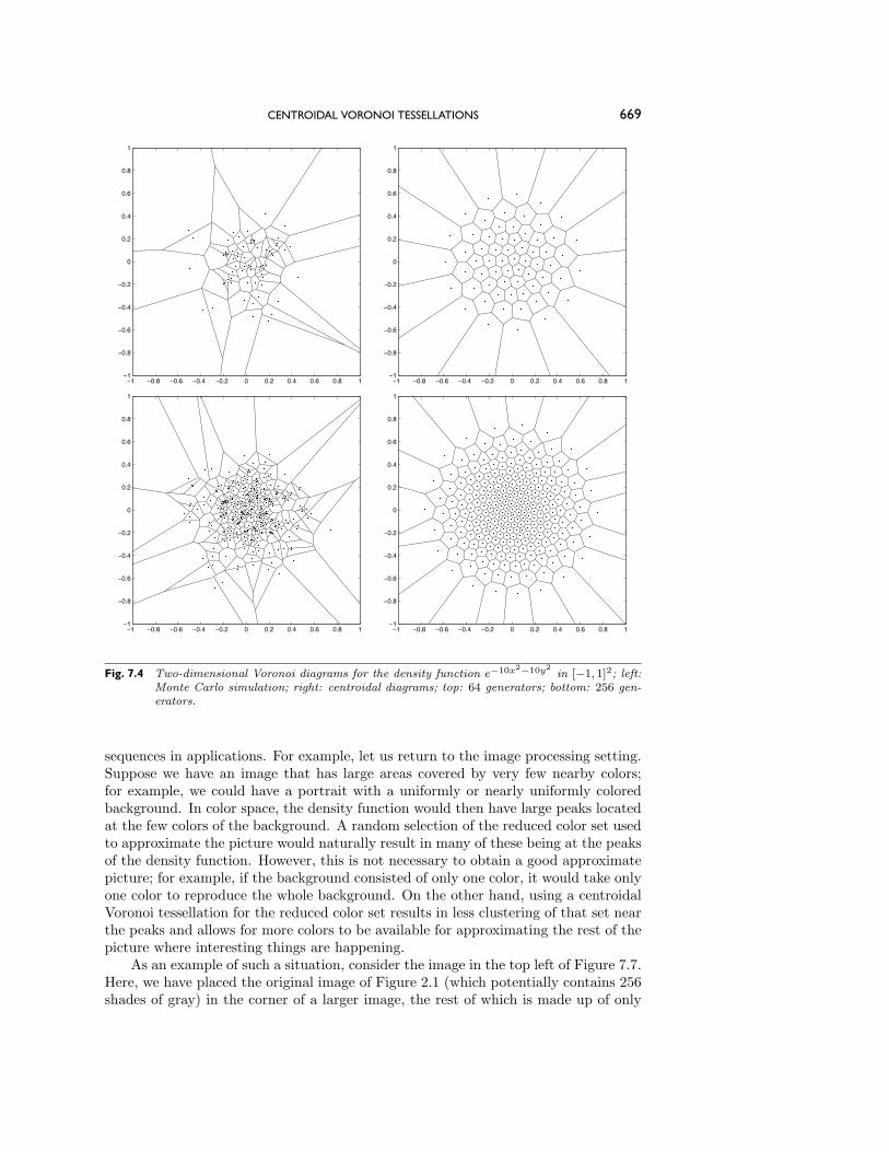
CENTROIDAL VORONOI TESSELLATIONS 669
−1 −0.8 −0.6 −0.4 −0.2 0 0.2 0.4 0.6 0.8 1−1
−0.8
−0.6
−0.4
−0.2
0
0.2
0.4
0.6
0.8
1
−1 −0.8 −0.6 −0.4 −0.2 0 0.2 0.4 0.6 0.8 1−1
−0.8
−0.6
−0.4
−0.2
0
0.2
0.4
0.6
0.8
1
−1 −0.8 −0.6 −0.4 −0.2 0 0.2 0.4 0.6 0.8 1−1
−0.8
−0.6
−0.4
−0.2
0
0.2
0.4
0.6
0.8
1
−1 −0.8 −0.6 −0.4 −0.2 0 0.2 0.4 0.6 0.8 1−1
−0.8
−0.6
−0.4
−0.2
0
0.2
0.4
0.6
0.8
1
Fig. 7.4 Two-dimensional Voronoi diagrams for the density function e−10x2−10y2in [−1, 1]2; left:
Monte Carlo simulation; right: centroidal diagrams; top: 64 generators; bottom: 256 gen-erators.
sequences in applications. For example, let us return to the image processing setting.Suppose we have an image that has large areas covered by very few nearby colors;for example, we could have a portrait with a uniformly or nearly uniformly coloredbackground. In color space, the density function would then have large peaks locatedat the few colors of the background. A random selection of the reduced color set usedto approximate the picture would naturally result in many of these being at the peaksof the density function. However, this is not necessary to obtain a good approximatepicture; for example, if the background consisted of only one color, it would take onlyone color to reproduce the whole background. On the other hand, using a centroidalVoronoi tessellation for the reduced color set results in less clustering of that set nearthe peaks and allows for more colors to be available for approximating the rest of thepicture where interesting things are happening.
As an example of such a situation, consider the image in the top left of Figure 7.7.Here, we have placed the original image of Figure 2.1 (which potentially contains 256shades of gray) in the corner of a larger image, the rest of which is made up of only
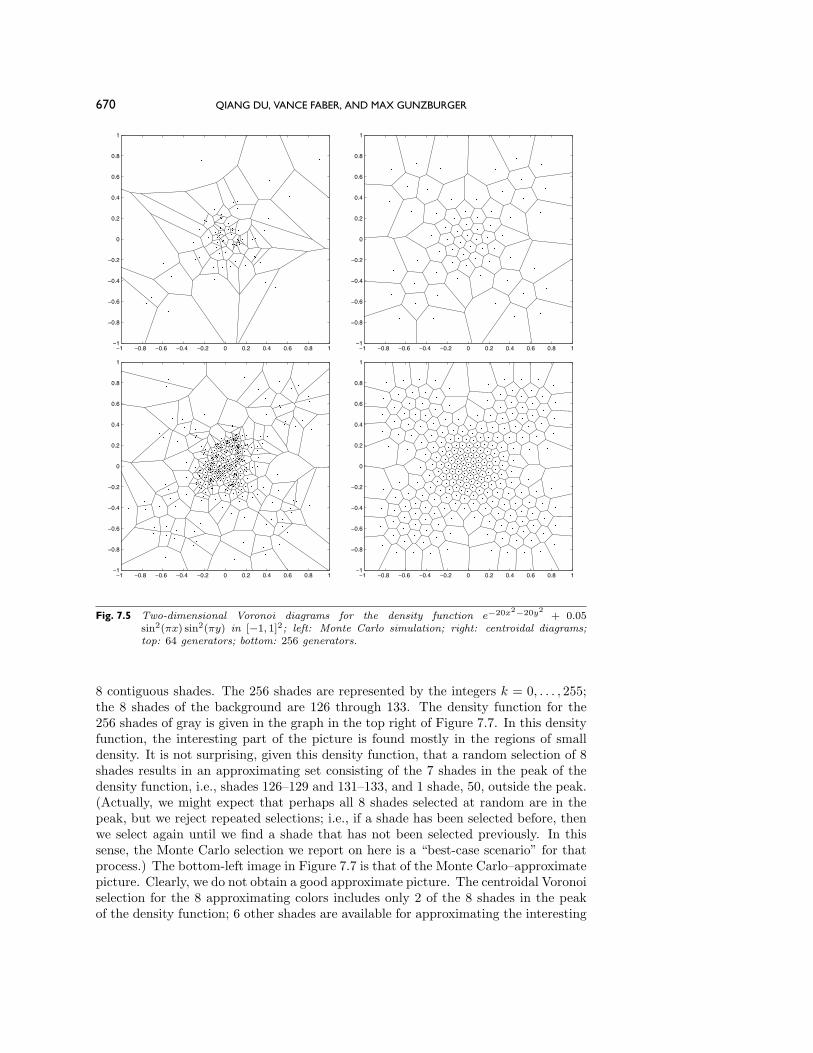
670 QIANG DU, VANCE FABER, AND MAX GUNZBURGER
−1 −0.8 −0.6 −0.4 −0.2 0 0.2 0.4 0.6 0.8 1−1
−0.8
−0.6
−0.4
−0.2
0
0.2
0.4
0.6
0.8
1
−1 −0.8 −0.6 −0.4 −0.2 0 0.2 0.4 0.6 0.8 1−1
−0.8
−0.6
−0.4
−0.2
0
0.2
0.4
0.6
0.8
1
−1 −0.8 −0.6 −0.4 −0.2 0 0.2 0.4 0.6 0.8 1−1
−0.8
−0.6
−0.4
−0.2
0
0.2
0.4
0.6
0.8
1
−1 −0.8 −0.6 −0.4 −0.2 0 0.2 0.4 0.6 0.8 1−1
−0.8
−0.6
−0.4
−0.2
0
0.2
0.4
0.6
0.8
1
Fig. 7.5 Two-dimensional Voronoi diagrams for the density function e−20x2−20y2+ 0.05
sin2(πx) sin2(πy) in [−1, 1]2; left: Monte Carlo simulation; right: centroidal diagrams;top: 64 generators; bottom: 256 generators.
8 contiguous shades. The 256 shades are represented by the integers k = 0, . . . , 255;the 8 shades of the background are 126 through 133. The density function for the256 shades of gray is given in the graph in the top right of Figure 7.7. In this densityfunction, the interesting part of the picture is found mostly in the regions of smalldensity. It is not surprising, given this density function, that a random selection of 8shades results in an approximating set consisting of the 7 shades in the peak of thedensity function, i.e., shades 126–129 and 131–133, and 1 shade, 50, outside the peak.(Actually, we might expect that perhaps all 8 shades selected at random are in thepeak, but we reject repeated selections; i.e., if a shade has been selected before, thenwe select again until we find a shade that has not been selected previously. In thissense, the Monte Carlo selection we report on here is a “best-case scenario” for thatprocess.) The bottom-left image in Figure 7.7 is that of the Monte Carlo–approximatepicture. Clearly, we do not obtain a good approximate picture. The centroidal Voronoiselection for the 8 approximating colors includes only 2 of the 8 shades in the peakof the density function; 6 other shades are available for approximating the interesting
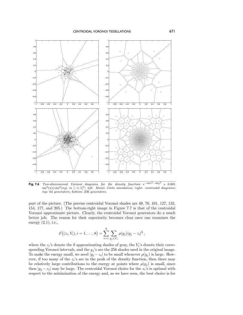
CENTROIDAL VORONOI TESSELLATIONS 671
−1 −0.8 −0.6 −0.4 −0.2 0 0.2 0.4 0.6 0.8 1−1
−0.8
−0.6
−0.4
−0.2
0
0.2
0.4
0.6
0.8
1
−1 −0.8 −0.6 −0.4 −0.2 0 0.2 0.4 0.6 0.8 1−1
−0.8
−0.6
−0.4
−0.2
0
0.2
0.4
0.6
0.8
1
−1 −0.8 −0.6 −0.4 −0.2 0 0.2 0.4 0.6 0.8 1−1
−0.8
−0.6
−0.4
−0.2
0
0.2
0.4
0.6
0.8
1
−1 −0.8 −0.6 −0.4 −0.2 0 0.2 0.4 0.6 0.8 1−1
−0.8
−0.6
−0.4
−0.2
0
0.2
0.4
0.6
0.8
1
Fig. 7.6 Two-dimensional Voronoi diagrams for the density function e−40x2−40y2+ 0.001
sin2(πx) sin2(πy) in [−1, 1]2; left: Monte Carlo simulation; right: centroidal diagrams;top: 64 generators; bottom: 256 generators.
part of the picture. (The precise centroidal Voronoi shades are 49, 76, 101, 127, 132,154, 177, and 205.) The bottom-right image in Figure 7.7 is that of the centroidalVoronoi approximate picture. Clearly, the centroidal Voronoi generators do a muchbetter job. The reason for their superiority becomes clear once one examines theenergy (2.1), i.e.,
E((zi, Vi), i = 1, . . . , 8) = 8∑i=1
∑yj∈Vi
ρ(yj)|yj − zi|2 ,
where the zi’s denote the 8 approximating shades of gray, the Vi’s denote their corre-sponding Voronoi intervals, and the yj ’s are the 256 shades used in the original image.To make the energy small, we need |yj− zi| to be small whenever ρ(yj) is large. How-ever, if too many of the zi’s are in the peak of the density function, then there maybe relatively large contributions to the energy at points where ρ(yj) is small, sincethen |yj − zi| may be large. The centroidal Voronoi choice for the zi’s is optimal withrespect to the minimization of the energy and, as we have seen, the best choice is for

672 QIANG DU, VANCE FABER, AND MAX GUNZBURGER
0 50 100 150 200 250 3000
1
2
3
4
5
6
7x 10
4 Color density distribution
Fig. 7.7 Top left: an 8-bit image embedded in a nearly uniform background. Top right: the gray scaledensity function for the image in the top left. Bottom left: the Monte Carlo compressed3-bit image. Bottom right: the centroidal Voronoi compressed 3-bit image.
two of the zi’s to be within the peak and for the other six to be distributed amongthose points at which the density is small.
The final figure is for a smoothly varying density having a maximum at a corner ofthe image; see Figure 7.8. Many of the features of the previous examples also appearin this figure. In particular, note that, in general, generators chosen according to acentroidal Voronoi tessellation result in much more uniform and symmetric tessella-tions which, at least to these authors, are more pleasing to the eye and which, as wehave seen, are also more useful.
8. Conclusions. There are numerous analytical and computational issues con-nected with centroidal Voronoi tessellations that warrant further examination. Amongthese are the following: How can Lloyd’s method be modified so that it has an accel-erated convergence rate? Can it be proved, for a constant density function, that theoptimal quantizer is given asymptotically by a uniform lattice in higher dimensionalspace? How can we find the centroidal Voronoi tessellations corresponding to theglobal minimum while avoiding local minima? What do centroidal Voronoi solutionsin non-Euclidean metrics look like and how can they be efficiently computed? Whatis the complexity of the local optimal quantizer problem? In this last regard, it wasshown in [13] that a simple case of the general local optimal quantizer problem is NP-complete. Thus, the general problem of communication theory, in its combinatorialforms, has at least that complexity.
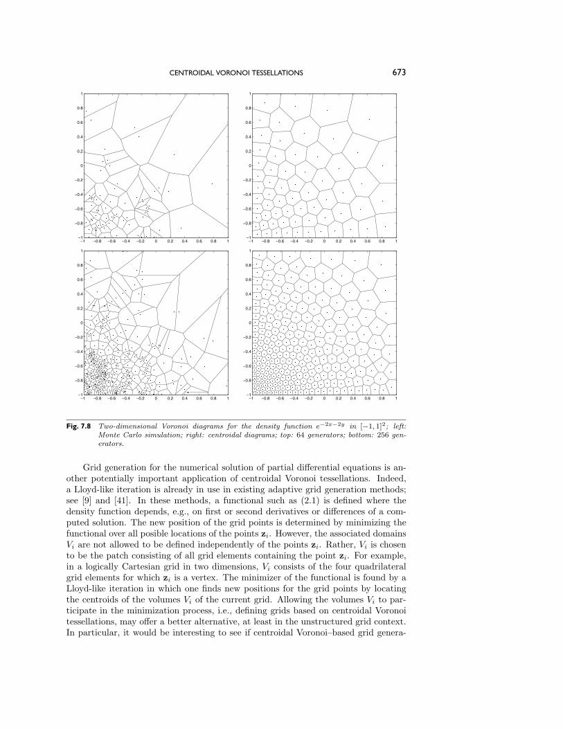
CENTROIDAL VORONOI TESSELLATIONS 673
−1 −0.8 −0.6 −0.4 −0.2 0 0.2 0.4 0.6 0.8 1−1
−0.8
−0.6
−0.4
−0.2
0
0.2
0.4
0.6
0.8
1
−1 −0.8 −0.6 −0.4 −0.2 0 0.2 0.4 0.6 0.8 1−1
−0.8
−0.6
−0.4
−0.2
0
0.2
0.4
0.6
0.8
1
−1 −0.8 −0.6 −0.4 −0.2 0 0.2 0.4 0.6 0.8 1−1
−0.8
−0.6
−0.4
−0.2
0
0.2
0.4
0.6
0.8
1
−1 −0.8 −0.6 −0.4 −0.2 0 0.2 0.4 0.6 0.8 1−1
−0.8
−0.6
−0.4
−0.2
0
0.2
0.4
0.6
0.8
1
Fig. 7.8 Two-dimensional Voronoi diagrams for the density function e−2x−2y in [−1, 1]2; left:Monte Carlo simulation; right: centroidal diagrams; top: 64 generators; bottom: 256 gen-erators.
Grid generation for the numerical solution of partial differential equations is an-other potentially important application of centroidal Voronoi tessellations. Indeed,a Lloyd-like iteration is already in use in existing adaptive grid generation methods;see [9] and [41]. In these methods, a functional such as (2.1) is defined where thedensity function depends, e.g., on first or second derivatives or differences of a com-puted solution. The new position of the grid points is determined by minimizing thefunctional over all posible locations of the points zi. However, the associated domainsVi are not allowed to be defined independently of the points zi. Rather, Vi is chosento be the patch consisting of all grid elements containing the point zi. For example,in a logically Cartesian grid in two dimensions, Vi consists of the four quadrilateralgrid elements for which zi is a vertex. The minimizer of the functional is found by aLloyd-like iteration in which one finds new positions for the grid points by locatingthe centroids of the volumes Vi of the current grid. Allowing the volumes Vi to par-ticipate in the minimization process, i.e., defining grids based on centroidal Voronoitessellations, may offer a better alternative, at least in the unstructured grid context.In particular, it would be interesting to see if centroidal Voronoi–based grid genera-

674 QIANG DU, VANCE FABER, AND MAX GUNZBURGER
tion can be used to avoid problems such as grid crossovers and slivers that occur inother grid generation methods.
Acknowledgments. The authors thank the editors and the reviewers of the paperfor their suggestions and comments, which have resulted in a substantial improvement.
REFERENCES
[1] E. Abaya and F. Wise, Convergence of vector quantizers with applications to optimal quan-tization, SIAM J. Appl. Math., 44 (1984), pp. 183–189.
[2] T. Asano, B. Bhattacharya, M. Keil, and F. Yao, Clustering algorithms based on mini-mum and maximum spanning trees, in Proceedings of the Fourth Annual Symposium onComputational Geometry, University of Illinois, Urbana, 1988, pp. 252–257.
[3] G. Barlow, Hexagonal territories, Animal Behav., 22 (1974), pp. 876–878.[4] G. Celeux and G. Govaert, A classification EM algorithm for clustering and two stochastic
versions, Comput. Statist. Data. Anal., 14 (1992), pp. 315–332.[5] C. Chinrungrueng and C. Sequin, Optimal adaptive k-means algorithm with dynamic ad-
justment of learning rate, IEEE Trans. Neural Net., 6 (1995), pp. 157–169.[6] R. Clark, Optisim—An extended dissimilarity selection method for finding diverse represen-
tative subsets, J. Chem. Inform. Comput. Sci., 37 (1997), pp. 1181–1188.[7] P. Davis and P. Rabinowitz, Methods of Numerical Integration, 2nd ed., Academic Press,
New York, 1984.[8] F. Denatale, G. Desoli, D. Giusto, and G. Vernazza, Polynomial approximation and vector
quantization—A region-based integration, IEEE Trans. Comm., 43 (1995), pp. 198–206.[9] P. Eiseman, Adaptive grid generation, Comput. Methods Appl. Mech. Engrg., 64 (1987), pp.
321–376.[10] R. England and D. Benyon, A remark on Algorithm AS136: k-means clustering algorithm,
Appl. Statist., 30 (1981), pp. 355–356.[11] J. Friedman, Exploratory projection pursuit, J. Amer. Statist. Assoc., 82 (1987), pp. 249–266.[12] M. Garey and D. Johnson, Computers and Intractability: A Guide to the Theory of NP-
Completeness, Freeman, San Francisco, 1979.[13] M. Garey, D. Johnson, and H. Witsenhausen, The complexity of the generalized Lloyd-Max
problem, IEEE Trans. Inform. Theory, 28 (1982), pp. 255–256.[14] A. Gersho, Asymptotically optimal block quantization, IEEE Trans. Inform. Theory, 25 (1979),
pp. 373–380.[15] A. Gersho and R. Gray, Vector Quantization and Signal Compression, Kluwer, Boston, 1992.[16] R. Gray, J. Kieffer, and Y. Linde, Locally optimal block quantizer design, Inform. and
Control, 45 (1980), pp. 178–198.[17] R. Gray and D. Neuhoff, Quantization, IEEE Trans. Inform. Theory, 44 (1998), pp. 2325–
2383.[18] P. Hall, On polynomial-based projection indices for exploratory projection pursuit, Ann.
Statist., 17 (1989), pp. 589–605.[19] J. Hartigan, Clustering Algorithms, Wiley-Interscience, New York, 1975.[20] J. Hartigan, Asymptotic distribution for clustering centers, Ann. Statist., 6 (1978), pp. 117–
131.[21] J. Hartigan and M. Wong, A k-means clustering algorithm, Appl. Statist. 28 (1979), pp.
100–108.[22] M. Hasegawa and M. Tanemura, On the pattern of space division by territories, Ann. Inst.
Statist. Math., 28 (1976), pp. 509–519.[23] M. Hasegawa and M. Tanemura, Spatial patterns of territories, Recent Developments in
Statistical Inference and Data Analysis, K. Matusita, ed., North–Holland, Amsterdam,1980, pp. 73–78.
[24] S. Hasegawa, H. Imai, M. Inaba, N. Katoh, and J. Nakano, Efficient algorithms forvariance-based k-clustering, in Proceedings of the First Pacific Conference on ComputerGraphics and Applications, World Scientific, River Edge, NJ, 1993, pp. 75–89.
[25] P. Heckert, Color image quantization frame buffer display, ACM Trans. Comput. Graph., 16(1982), pp. 297–304.
[26] F. Hickernell and H. Hong, The asymptotic efficiency of randomized nets for quadrature,Math. Comp., 68 (1999), pp. 767–791.
[27] H. Honda, Description of cellular patterns by Dirichlet domains: The two-dimensional case,J. Theoret. Biol., 72 (1978), pp. 523–543.
[28] H. Honda, Geometrical modelling for cells in tissues, Inter. Rev. Cytol., 81 (1983), pp. 191–248.
CENTROIDAL VORONOI TESSELLATIONS 675
[29] P. Huber, Projection pursuit, with discussion, Ann. Statist., 13 (1985), pp. 435–525.[30] H. Imai and M. Inaba, Geometric k-clustering with applications, in Proceedings of the Third
International Congress of Industrial and Applied Mathematics, 1995, to appear.[31] H. Imai, N. Katoh, and M. Inaba, Applications of weighted Voronoi diagrams and ran-
domization to variance-based k-clustering, Proceedings of the 10th ACM Symposium onComputational Geometry, 1994, pp. 332–339.
[32] M. Inaba, H. Imai, and N. Katoh, Experimental results of randomized clustering algorithms,in Proceedings of the 12th ACM Symposium on Computational Geometry: CommunicationSection, 1996, to appear.
[33] M. Iri, K. Murota, and T. Ohya, A fast Voronoi-diagram algorithm with applications togeographical optimization problems, in Proceedings of the 11th IFIP Conference on SystemModelling and Optimzation, Lecture Notes in Control and Inform. Sci. 59, Springer-Verlag,New York, pp. 273–288.
[34] A. Jain and R. Dubes, Algorithms for Clustering Data, Prentice–Hall, Englewood Cliffs, NJ,1998.
[35] M. Jhun, Bootstrapping k-means clustering, J. Japanese Soc. Comput. Statist., 3 (1990), pp.1–14.
[36] J. Kieffer, Uniqueness of locally optimal quantizer for log-concave density and convex errorfunction, IEEE Trans. Inform. Theory, 29 (1983), pp. 42–47.
[37] R. Klein, Concrete and Abstract Voronoi Diagrams, Lecture Notes in Comput. Sci. 400,Springer, New York, 1989.
[38] Y. Linde, A. Buzo, and R. Gray, An algorithm for vector quantizer design, IEEE Trans.Comm., 28 (1980), pp. 84–95.
[39] S. Lloyd, Least square quantization in PCM, IEEE Trans. Inform. Theory, 28 (1982), pp.129–137.
[40] J. MacQueen, Some methods for classification and analysis of multivariate observations, inProceedings, Fifth Berkeley Symposium on Mathematical Statistics and Probability, Vol.I, L. Le Cam and J. Neyman, eds., University of California, Berkeley, 1967, pp. 281–297.
[41] D. McRae and K. Laflin, Dynamic grid adaptation and grid quality, in CRC Handbook ofGrid Generation, CRC, Boca Raton, FL, 1998, pp. 34-1–33.
[42] V. Mathews, Vector quantization of images using the l∞ distortion measure, IEEE SignalProc. Lett., 5 (1997), pp. 33–35.
[43] U. Moller, M. Galicki, E. Baresova, and H. Witte, An efficient vector quantizer providingglobally optimal-solutions, IEEE Trans. Signal Proc., 46 (1998), pp. 2515–2529.
[44] D. Newman, The hexagon theorem, IEEE Trans. Inform. Theory, 28 (1982), pp. 137–139.[45] R. Nicolaides, Direct discretization of planar div-curl problems, SIAM J. Numer. Anal., 29
(1992), pp. 32–56.[46] H. Niederreiter, Random Number Generation and Quasi-Monte Carlo Methods, SIAM,
Philadelphia, 1992.[47] A. Okabe, B. Boots, and K. Sugihara, Spatial Tessellations; Concepts and Applications of
Voronoi Diagrams, Wiley, Chichester, UK, 1992.[48] C. Papadimitriou and K. Steiglitz, Combinatorial Optimization: Algorithms and Complex-
ity, Prentice–Hall, Englewood Cliffs, NJ, 1982.[49] A. Papageorgiou and J. Traub, Fast evaluation of multidimensional integrals, Comput.
Phys., 11 (1997), pp. 574–579.[50] K. Parna, Strong consistency of k-means clustering criterion in separable metric spaces, Tartu
Riikl. Ul. Toimetised, 733 (1986), pp. 86–96.[51] K. Parna, On the stability of k-means clustering in metric spaces, Tartu Riikl. Ul. Toimetised,
798 (1988), pp. 19–36.[52] D. Pollard Strong consistency of k-mean clustering, Ann. Statist., 9 (1981), pp. 135–140.[53] D. Pollard, A central limit theorem for k-means clustering, Ann. Statist., 10 (1982), pp.
919–926.[54] F. Preparata and M. Shamos, Computational Geometry—An Introduction, Springer, New
York, 1985.[55] S. Selim and M. Ismail, K-means-type algorithms: A generalized convergence theorem and
characterization of local optimality, IEEE Trans. Pattern Anal. Mach. Intell., PAMI-6(1984), pp. 81–87.
[56] W. Sheppard, On the calculation of the most probable values of frequency constants for dataarranged according to equidistant divisions of a scale, Proc. London Math. Soc., 24 (1898),pp. 353–390.
[57] I. Sloan and H. Wozniakowski, When are quasi-Monte Carlo algorithms efficient for high-dimensional integrals?, J. Complexity, 14 (1998), pp. 1–33.

676 QIANG DU, VANCE FABER, AND MAX GUNZBURGER
[58] W. Stute and L. Zhu, Asymptotics of k-means clustering based on projection pursuit, SankhyaSer. A, 57 (1995), pp. 462–471.
[59] A. Suzuki and M. Iri, Approximation of a tessellation of the plane by a Voronoi diagram, J.Oper. Res. Soc. Japan, 29 (1986), pp. 69–96.
[60] M. Tanemura and M. Hasegawa, Geometrical models of territory. I. Models for synchronousand asynchronous settlement of territories, J. Theoret. Biol., 82 (1980), pp. 477–496.
[61] A. Trushkin, On the design of an optimal quantizer, IEEE Trans. Inform. Theory, 39 (1993),pp. 1180–1194.
[62] S. Wan, S. Wong, and P. Prusinkiewicz, An algorithm for multidimensional data clusteringACM Trans. Math. Software, 14 (1988), pp. 153–162.
[63] M. Wong, Asymptotic properties of univariate sample k-means clusters, J. Classification, 1(1984), pp. 255–270.
[64] X. Wu and I. Witten, A Fast k-Means Type Clustering Algorithm, Tech. Report, Departmentof Computer Science, University of Calgary, Alberta, Canada, 1985.