arX

iv:1

203.

0478

v1 [

cs.C

G]

2 M

ar 2

012

Certified Approximation of Parametric Space Curves

with Cubic B-spline Curves

Liyong Shena, Chun-Ming Yuanb, Xiao-Shan Gaob

aSchool of Mathematical Sciences, Graduate University of Chinese Academy of SciencesbKey Laboratory of Mathematics Mechanization, AMSS, Chinese Academy of Sciences

Abstract

Approximating complex curves with simple parametric curves is widely used in CAGD,CG, and CNC. This paper presents an algorithm to compute a certified approximation toa given parametric space curve with cubic B-spline curves. By certified, we mean that theapproximation can approximate the given curve to any given precision and preserve thegeometric features of the given curve such as the topology, singular points, etc. The approx-imated curve is divided into segments called quasi-cubic Bezier curve segments which haveproperties similar to a cubic rational Bezier curve. And the approximate curve is naturallyconstructed as the associated cubic rational Bezier curve of the control tetrahedron of aquasi-cubic curve. A novel optimization method is proposed to select proper weights in thecubic rational Bezier curve to approximate the given curve. The error of the approximationis controlled by the size of its tetrahedron, which converges to zero by subdividing the curvesegments. As an application, approximate implicit equations of the approximated curvescan be computed. Experiments show that the method can approximate space curves of highdegrees with high precision and very few cubic Bezier curve segments.

Keywords: Space parametric curve, certified approximation, geometric feature, cubicBezier curve, cubic B-spline curve.

1. Introduction

Parametric curves are widely used in different fields such as computer aided geometricdesign (CAGD), computer graphics (CG), computed numerical control (CNC) systems [1, 2].One basic problem in the study of parametric curves is to approximate the curve withlower degree curve segments. For a given digital curve, there exist methods to find suchapproximate curves efficiently [3, 4, 5, 6]. If the curve is given by explicit expressions,either parametric or implicit, these methods are still usable. However, some importantgeometric features such as singular points cannot be preserved. In this paper, we will focuson computing approximate curves which can approximate the given curve to any precision

Email addresses: shenly@amss.ac.cn (Liyong Shen), cmyuan@mmrc.iss.ac.cn (Chun-Ming Yuan),xgao@mmrc.iss.ac.cn (Xiao-Shan Gao)

Preprint submitted to Elsevier March 5, 2012

and preserve the topology and certain geometric features of the given space curve. Suchan approximate curve is called a certified approximation. Here, the geometric featuresinclude cusps, self-intersected points, inflection points, torsion vanishing points, as well asthe segmenting points and the left(right) Frenet frames of these points.

There are lots of papers tried to approximate a smooth parametric curve segment [1,7, 8, 9, 10, 11, 12, 13, 14]. Among them, Geometric Hermite Interpolation (GHI) is atypical method for the curve approximation. Degen [8] presented an overview over thedevelopments of geometric Hermite approximation theory for planar curves. Several 2Dinterpolation schemes to produce curves close to circles were proposed in [9]. The certifiedapproximation were considered by some authors and they focused on the case of planarcurves [15, 16, 17, 18].

For space curves, Hijllig and Koch [10] improved the standard cubic Hermite interpolationwith approximation order five by interpolating a third point. Xu and Shi [11] consideredthe GHI for space curves by parametric quartic Bezier curve. Pelosi et al. [12] discussed theproblem of Hermite interpolation by using PH cubic segments. Chen et al. [14] enhancedthe GHI by adding an inner tangent point and the approximation was then more accurate.These methods were mainly designed for the local approximation of a parametric curvesegment. The approximate curves obtained generally cannot preserve geometric featuresand topologies for the global approximation. The algorithms had to be improved to meetcertain special conditions. For instance, Wu et al [19] presented an algorithm to preserve thetopology of voxelisation and Chen et al [20] gave the formula of the intersection curve of tworuled surfaces by the bracket method. As a further development for certified approximation,more properties such as the topology and singularities of the curve need to be discussedin the approximation process. We would like to give the local approximation with certainrestrictions. And the local approximation methods can then be used in the global certifiedapproximation naturally.

The certified approximation is also based on the topology determination. For implicitcurves, the problem of topology determination was studied in some papers such as [21, 22,23, 24]. Efficient algorithms were proposed in [25] and [26] to compute the real singularpoints of a rational parametric space curve by the µ-basis method and the generalized D-resultant method respectively. An algorithm was proposed to compute the topology for arational parametric space curve [27]. However, even we have the methods to determine thetopology of space curves and the methods to approximate the space curves with free formcurves, the combination of them is not straightforward. The topology may change whilethe line edges in topology graph are replaced by the approximate free form curve segments.For example, some knots may be brought in or lost such that the crossing number of theapproximate curve is not equivalent to the approximated curve.

In this paper, we compute a certified approximation to a given parametric space curvewith a rational cubic B-spline curve based on the topology. The cubic rational Bezier curveis taken as the approximate curve segment because it is the simplest non-planar curve andhas nice properties [28, 29]. The presented method consists of two major steps.

In the first step, the given space curve segment is divided into sub-segments which havesimilar properties to a cubic rational Bezier curve. Such curve segments are called quasi-

2

cubic Bezier curves. The preliminary work of our division procedure is to compute thesingular points and the topology graph of the given curve, which have already been studiedin [30, 25, 26, 27]. Inflection points and torsion vanishing points of the curve are also added ascharacter points. We further divide the curve segments to ensure that the subdivided curvesegments have similar properties to a cubic Bezier curve. For instance, each curve segmenthas an associated control tetrahedron whose four vertices consist of the two endpoints ofthe curve segment and the two intersection points of the tangent lines and the osculatingplanes at the different endpoints respectively. And the curve segment is inside its associatedcontrol tetrahedron. Furthermore, we need to ensure some monotone properties about theassociated control tetrahedron, which are necessary for the convergence of the algorithm.The tetrahedrons are then just the control polytope of the approximate cubic Bezier curves.In other words, the approximate curve is controlled by the sequence of the tetrahedrons.And this property ensure the topological isotopy for the approximated and approximatecurves. Some more careful discussions are proposed for both cubic Bezier and quasi-cubiccurve segments.

In the second step of the algorithm, we use a cubic rational Bezier spline to approximatea quasi-cubic Bezier curve obtained in the first step. Some different approximation methodscan be used here such as GHI with inner tangent points [14]. However, as we mentioned, aquasi-cubic Bezier curve has an associated control tetrahedron. The associated cubic rationalBezier curve of this tetrahedron is naturally used as the approximate curve. So, each curvesegment and its approximated cubic curve segment share the same control tetrahedron.A novel method, called shoulder point approximation, is proposed to select parameters inthe cubic Bezier curve so that it can optimally approximate the given curve segment. Ifthe distance between the two curve segments is larger than the given precision, we furthersubdivide the given curve segment and approximate each sub-segment similarly. The errorof the approximation is controlled by the size of the associated tetrahedrons, which areproved to converge to zero. In the subdivision process, there is one important differencebetween our algorithm with the others. We only need to check the collision of the sub-tetrahedrons subdivided from which are the intersected before the subdivision, since thesub-tetrahedrons are included in its father tetrahedrons. In general algorithms, one has tocheck the collision of all pair of the approximate curve segments or their control polytopesafter a subdivision. Finally, the rational cubic Bezier curves are converted to a C1 rationalB-spline with a proper knot selection and used as the final approximate curve. After a cubicparametric approximate segment is computed, we can compute its algebraic variety usingthe µ-basis method [31], which can be used as the approximate implicit equations for thegiven parametric curve.

The proposed method is implemented and experimental results show that the methodcan be used to compute certified approximate curves to high degree space curves efficiently.The computed rational B-spline has very few pieces and can approximate the given curveswith high precision.

The rest of this paper is organized as follows. In Section 2, some notations and prelimi-nary results are given. In Section 3, we give the algorithm to compute the dividing pointssuch that each divided segment is a quasi-cubic curve. In Section 4, the method of parameter

3

selection for the cubic rational Bezier segments is proposed and then an algorithm basedon shoulder point approximation is given. We also prove that the termination of the algo-rithm. The final algorithm is given in Section 5, and some examples are used to illustratethe algorithm. In section 6, the paper is concluded.

2. Preliminaries

Basic notations and preliminary results about rational parametric curves and cubic Beziercurves are presented in this section.

2.1. Basic notations

A parametric space curve is defined as

r(t) = (x(t), y(t), z(t)), (2.1)

where x(t), y(t), z(t) ∈ Q(t) and Q is the field of rational numbers. In the univariate case,Luroth’s theorem provides a proper reparametrization algorithm and some improved algo-rithms which can also be found such as [30]. So we assume that (2.1) is a proper parametriccurve in an interval [0, 1] since any interval [a, b] can be transformed to [0, 1] by a parametrictransformation t ← t−a

b−a. Further, the denominators of (2.1) are assumed to have no real

roots in [0, 1].The tangent vector of r(t) is r′(t) = (x′(t), y′(t), z′(t)) and the tangent line of r(t) at a

point r(t0) is T(t0) = r(t0) + λr′(t0), λ ∈ Q. A point r(t0) is called a singular point if itcorresponds to more than one parameters with multiplicities counted. A singular point iscalled a cusp if r′(t0) is the vector of zeros, which means that t0 is a multiple parameter;otherwise, it is an ordinary singular point [26]. The curvature and torsion of the curve are

κ(t) =‖r′(t)× r′′(t)‖

‖r′(t)‖3, τ(t) =

(r′, r′′, r′′′)

‖r′ × r′′‖.

A point is called an inflection if its curvature is zero and called torsion vanishing point ifits torsion is zero. All these points are called character points of the curve, and r(t) is anormal curve if it has a finite number of character points. A rational space curve is alwaysa normal curve. In this paper, we assume that κ(t) 6≡ 0 and τ(t) 6≡ 0, which means that thecurve is not a planar curve.

If r(t0) is not a character point, then the Frenet frame at r(t0) can be defined as F(t0) :=

{r(t0);α(t0),β(t0),γ(t0)} where α(t0) =r′(t0)

‖r′(t0)‖, β(t0) = γ(t0)×α(t0), γ(t0) =

r′(t0)×r

′′(t0)‖r′(t0)×r′′(t0)‖

are the unit tangent vector, unit principal normal vector, and unit bi-normal vector, respec-tively. And the osculating plane is O(t0) := ((x, y, z)− r(t0)) · γ(t0) = 0.

For a point with κ(t0) = 0, the bi-normal vector is not defined, neither is the osculatingplane. Here, we define them using limit. Consider the limit limt→t0 γ(t) of the bi-normalvector at t0. Since the left limit and the right limit are generally different, we define the leftbi-normal vector and the right bi-normal vector as γ−(t0) := limt→t0−0 γ(t) and γ+(t0) :=limt→t0+0 γ(t) respectively. The limitations always exist if r(t) is a rational space curve

4

of form (2.1). As a consequence, the left and right osculating planes at t0 are O−(t0) :=((x, y, z)− r(t0)) ·γ

− = 0 and O+(t0) := ((x, y, z)− r(t0)) ·γ+ = 0. If the κ(t0) 6= 0, one can

find that γ+(t0) = γ−(t0) and O+(t0) = O−(t0).Similarly, if t0 is at a cusp, we define the left and right tangent vectors as α−(t0) :=

limt→t0−0α(t) and α+(t0) := limt→t0+0α(t), respectively. Hence, the corresponding left andright principal vectors are β−(t0) := γ−(t0) × α−(t0) and β+(t0) := γ+(t0) × α+(t0). Wealso denote the left and right tangent lines as T−(t0) = r(t0) + λα−(t0) and T+(t0) =r(t0) + λα+(t0) where λ is the real number parameter. Then, a rational parametric curver(t) always has left and right Frenet frames.

2.2. Rational cubic Bezier curve

A rational Bezier curve with degree n has the following form

p(t) =

∑ni=0 ωipiB

ni (t)

∑ni=0 ωiBn

i (t), t ∈ [0, 1],

where ωi ≥ 0 are associated weights of the control points pi ∈ R3 and Bni (t) =

(

ni

)

(1−t)n−iti.When n = 3, it defines a cubic rational Bezier curve where ♦p0p1p2p3 is called the controltetrahedron of p(t). One can set the weight ω0 = ω3 = 1 up to a parametric transformation.We now consider the cubic curve and omit superscript 3 from B3

i (t)

p(t) =p0B0(t) + ω1p1B1(t) + ω2p2B2(t) + p3B3(t)

B0(t) + ω1B1(t) + ω2B2(t) +B3(t), t ∈ [0, 1]. (2.2)

The rational cubic Bezier curve (2.2) has the following properties.

Lemma 2.1. Let p(t) be a non-planar cubic rational curve of the form (2.2). Then

1) p(t) passes through the endpoints p0,p3 with the corresponding tangent directions p′(0)and p′(1) parallel to p0p1 and p2p3 respectively.

2) p0p1p2 and p1p2p3 are the osculating planes of p(t) at the endpoints p0 and p3, respec-tively.

3) p(t) lies inside its control tetrahedron ♦p0p1p2p3.

4) p(t) has no singular points and κ(t) 6= 0, τ(t) 6= 0 in [0, 1].

5) For any t⋆1 < t⋆2 ∈ [0, 1], the control tetrahedron of p⋆(t) = p(t), t ∈ [t⋆1, t⋆2] is inside the

control tetrahedron of p(t) .

6) ‖p0p01‖, ‖p1p12‖, and ‖p2p23‖ are strictly monotone for t⋆ ∈ (0, 1) where p01,p12, andp23 are the intersection points of the osculating plane O(t⋆) with p0p1,p1p2, and p2p3

respectively.

7) ‖p0p03‖ and ‖p1p12‖ are strictly monotone for t⋆ ∈ (0, 1) where p03 = p1p2p(t⋆)⋂

p0p3

and p12 = p0p3p(t⋆)⋂

p1p2.

5

Proof. Properties 1), 2) and 3) are basic properties of Bezier curves and the proof can befounded in [1]. They also can be checked directly.

For 4), Li and Cripps shown that there is no cusps and inflection points for a non-degenerate rational cubic space curves in [32], and the torsion can be checked directly.Wang et al. also proved that a cubic space curve has no singular points by moving planesmethod in [25].

5) can be proved by a successive Decasteljau subdivision [1]. The control tetrahedron ofp⋆1(t), t ∈ [t⋆1, 1] is inside the control tetrahedron of p(t). Successively, the control tetrahedron

of p⋆(t), t ∈ [t⋆1, t⋆2] lies in the control tetrahedron of p⋆

1(t).Property 6) can be derived from the above five properties. Also this property is a special

case of the following Theorem 3.10 in this paper.For 7), it is sufficient to prove that the planes p1p2p(t

⋆) and p0p3p(t⋆) do not touch

p(t⋆) with t⋆ ∈ (0, 1), respectively. Since p0p3p(t⋆) passes through p0,p3 and p(t) is cu-

bic, p0p3p(t⋆) cannot have any tangent point different from p0,p3. Supposing the plane

p1p2p(t⋆) touches p(t⋆) at t⋆ ∈ (0, 1), the osculating plane O(t⋆) must intersects p1p2p(t

⋆)with the tangent line T(t⋆). By 6), T(t⋆) must intersect p1p2 which is the intersection lineof O(0), O(1). However, according to Decasteljau subdivision, the intersection point of T(t⋆)and O(0) is always different from that of T(t⋆) and O(1). Then there is a contradiction. �

The shoulder point of a cubic Bezier curve will play an important role [28]. The definitionis given below.

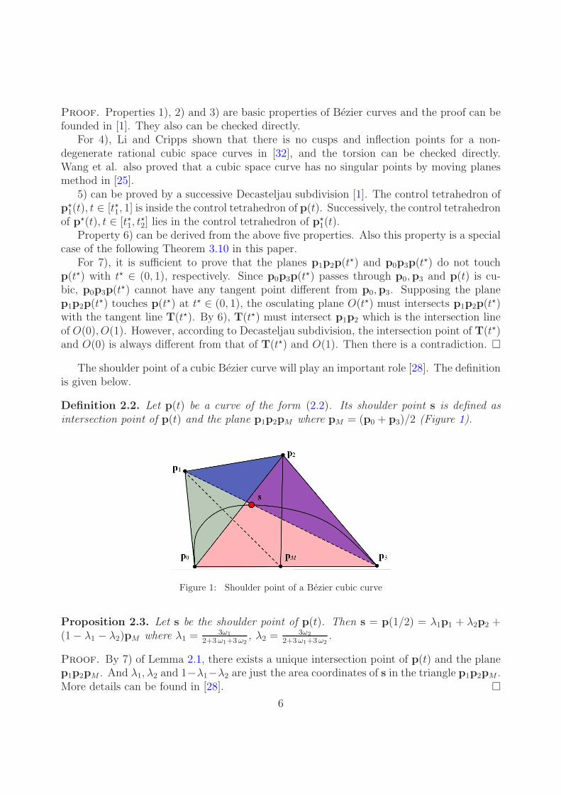
Definition 2.2. Let p(t) be a curve of the form (2.2). Its shoulder point s is defined asintersection point of p(t) and the plane p1p2pM where pM = (p0 + p3)/2 (Figure 1).

Figure 1: Shoulder point of a Bezier cubic curve

Proposition 2.3. Let s be the shoulder point of p(t). Then s = p(1/2) = λ1p1 + λ2p2 +(1− λ1 − λ2)pM where λ1 =

3ω1

2+3ω1+3ω2, λ2 =

3ω2

2+3ω1+3ω2.

Proof. By 7) of Lemma 2.1, there exists a unique intersection point of p(t) and the planep1p2pM . And λ1, λ2 and 1−λ1−λ2 are just the area coordinates of s in the triangle p1p2pM .More details can be found in [28]. �

6

It is known that the curve is closer to the control point when its associated weightis greater. We now consider the point which has the maximum distance to the planesP1 = p0p2p3 and P2 = p0p1p3 respectively.

Definition 2.4. Let r(t), t ∈ [0, 1] be a curve segment on the same side of a plane Q withthe two endpoints on Q. For another plane R parallel to Q, a tangent point of r(t) with theplane R is called a parallel point of r(t) associated to the plane Q.

According to the definition, a parallel point should satisfy

|r′(t),q1 − q0,q2 − q0| = 0, (2.3)

where q0,q1 and q2 are three non co-linear points on Q. In general, there may be severalparallel points for a curve segment and a fixed plane. However, for the rational cubic curvesegment (2.2), there is a unique parallel point associated to P1 = p0p2p3, and similarly,there is a unique parallel point associated to P2 = p0p1p3.

Proposition 2.5. Let p(t) be a non-planar cubic rational curve of the form (2.2). Thenthere are unique parallel points associated to the planes P1 and P2 respectively, and they arepoints of p(t) having the maximal distance to P1 and P2 respectively.

Proof. By equation (2.3), we can find that 3t3−6t2+6t−23t(t−1)2

= ω1 and 3t3−3t2+3t−13t2(t−1)

= ω2 are theconstraint equations for the parallel points associated to P1 and P2 respectively. They aretwo monotone functions for t ∈ (0, 1) with two asymptotes t = 0, 1. It means that for anyweights there is only one parallel point associated to Pi. Furthermore, the parallel point hasthe maximal distance since the endpoints of the curve are on Pi. �

3. Quasi-cubic segments on space parametric curves

In this section, we propose a method to divide a given curve r(t) into segments whichhave similar properties to cubic Bezier curves, which are called quasi-cubic Bezier segmentsand can be approximated by cubic rational Bezier curves nicely.

3.1. Conditions for subdivision

Let t0, t1 be the endpoints of a curve segment r(t). We will define an associated tetrahe-dron for it. Let O+(t0) and O−(t1) be the right and left osculating planes at the endpointsrespectively. We denote their intersection line as L, if they are not parallel. Since L and theright tangent line T+(t0) are coplanar, they intersect at a point r1 if they are not parallel.Similarly, L and the right tangent line T−(t1) intersect at a point r2 if they are not parallel.So we obtain an associated tetrahedron ♦(t0, t1) = ♦r0r1r2r3 where r0 = r(t0) and r3 = r(t1)if r1 6= r2.

We have shown that a cubic Bezier curve segment has eight properties in Lemma 2.1and Proposition 2.5. In the following, we will show how to divide any given rational curvesegment into sub-segments having similar properties.

7

Definition 3.1. A curve segment is called a quasi-cubic Bezier curve segment, or simply aquasi-cubic segment, if it has the eight properties in Lemma 2.1 and Proposition 2.5.

Theorem 3.2. Given r(t) and t0, there always exists t1 > t0 such that r(t), t ∈ [t0, t1] is aquasi-cubic Bezier curve segment.

We leave the proof of this theorem at the end of the subsection 3.2.

Definition 3.3. Let r(t), t ∈ [t0, t1] be a quasi-cubic segment. Then its associated cubicBezier curve segment is defined by the associated tetrahedron of r(t), i.e., the control pointsare r0, r1, r2 and r3.

In order to divide the curve segment into quasi-cubic segments, we first add the inflectionpoints and torsion vanishing points as the dividing points, denoted by P. The parametersof these points can be computed by solving the real roots of κ(t)τ(t) = 0. The left and rightFrenet frames are also needed. There are several efficient methods to find the real roots ofa univariate polynomial [33, 34] and one can use the procedures realroot and isolate inMaple.

We need to find more dividing points. Fix a start point t = t0, we now try to determine t1such that t1−t0 is as big as possible and the segment is included in its associated tetrahedrondesigned above. Several boundary parametric values to exclude some special points withrespect to t0 are computed in the following cases:

Condition I). Let t⋆1 > t0 be its nearest parametric value from P. Find t1 ∈ (t0, t⋆1)

such that F1(s1, s2) := α+(s1) · γ−(s2) 6= 0 and F2(s1, s2) := α−(s2) · γ

+(s1) 6= 0 for anyt0 ≤ s1 < s2 ≤ t1, meaning that the right tangent vector α+(s1) is not parallel to theleft osculating plane O−(s2) and the left tangent vector α−(s2) is not parallel to the leftosculating plane O+(s1).

Since the curve is non-planar, Fi(s1, s2), i = 1, 2 cannot be identically zero. We takea further look at the inequalities F1 6= 0, F2 6= 0. Since the derivative can be computedusing limits, r(t) is differentiable to any order although the left and right derivative may bedifferent. For conveniences, we omit the +,− marks to distinguish between left and rightderivatives. In what below, we give detailed analysis for F1 and the analysis of F2 is similar.

F1(s1, s2) = α(s1) · γ(s2) =|r′(s1), r

′(s2), r′′(s2)|

‖r′(s1)‖‖r′(s2)× r′′(s2)‖.

Assuming s1 = t0 + δ1, s2 = s1 + δ2, δ1 ≥ 0, δ2 > 0, F1(s1, s2) is re-parameterized as

F1(δ1, δ2) =|r′(t0 + δ1), r

′(t0 + δ1 + δ2), r′′(t0 + δ1 + δ2)|

‖r′(t0 + δ1)‖‖r′(t0 + δ1 + δ2)× r′′(t0 + δ1 + δ2)‖.

Expanding the vectors of the numerator at t = t0+δ1 as Taylor series r′S(t0+δ1), r

′S(t0+δ1+δ2)

and r′′S(t0 + δ1 + δ2) respectively, and combining them, we have

F1(δ1, δ2) =δ22|r

′S(t0 + δ1), r

′′S(t0 + δ1 + δ2), r

′′′S (t0 + δ1 + δ2)|

‖r′(t0 + δ1)‖‖r′(t0 + δ1 + δ2)× r′′(t0 + δ1 + δ2)‖, (3.1)

8

where r′′S(t0 + δ1 + δ2) = (r′S(t0 + δ1 + δ2)− r′S(t0 + δ1))/δ2 and r′′′S (t0 + δ1 + δ2) = (r′′(t0 +δ1 + δ2) − r′′S(t0 + δ1 + δ2))/δ2. Furthermore, when δ2 = 0, r′′S(t0 + δ1) = r′′S(t0 + δ1) andr′′′S (t0 + δ1) = r′′′S (t0 + δ1).

Let f1(δ1, δ2) = F1(δ1, δ2)/δ22. Then f1(δ1, 0) = τ(t0 + δ1)/‖r

′(t0 + δ1)‖. F1(δ1, δ2) = 0 isa planar curve in the plane of (δ1, δ2) which has two components: a double line δ22 = 0 andanother planar curve f1(δ1, δ2) = 0. That means f1 = 0 intersects δ2 = 0 with the pointswhich are exactly the torsion vanishing points τ(t0 + δ1) = 0 of r(t). And we need notcompute these points since they are already included in the separating points needed in thetopology computation which is discussed in Section 3.3. Consider the intersection points off1(δ1, δ2) and δ1 = 0. We can find that the real roots of f1(0, δ2) = 0 are associated to thevector α(s1) = r′(t0) just parallelling to the osculating plane O(s2) = O(t0 + δ2).

Thus, condition I) can be reduced to solve the following optimization problem

min δ1 + δ2s.t. F1(δ1, δ2) = 0, δ1 ≥ 0, δ2 > 0

(3.2)

and then t1 can be selected from (t0, t0+ δ1+ δ2). There are numerical methods to solve theoptimization problem. However, we prefer to solve it based on the above discussion sinceit is enough to get a boundary parametric value less than the exact solution of (3.2). Wecan find the positive real roots of f1(δ1, 0) and f1(0, δ2) for δ1 and δ2 respectively. Let δ⋆1 bethe minimal one among all the real roots. Then δ1 + δ2 = δ⋆1 defines a line. If the line doesnot intersect f1 in the first quadrant, then t1 can be in (t0, t0 + δ⋆1). This can be checked byfinding the real roots of f1(δ

⋆1 − δ2, δ2) = 0. Otherwise, set δ⋆1 ← δ⋆1/2 and check the process

repeatedly until the proper δ⋆1 is found. If f1(δ1, 0) and f1(0, δ2) have no positive real roots,δ⋆1 can be initialed as δ⋆1 = t⋆1 − t0.

Similarly, we can find such a δ⋆2 for F2. Finally, let t⋆2 = min(t0 + δ⋆1, t0 + δ⋆2) be theboundary parametric value of t1.

Remark 3.4. The function F1(δ1, δ2) in (3.1) actually has a finite number of terms if theapproximated curve r is a rational curve. If r is a parametric curve in elementary functions,F1(δ1, δ2) will be in the series form. However, the problem (3.2) can still be solved usinga numerical method. Starting with an initial value δ⋆1, we can find a boundary number bychecking whether δ1 + δ2 = δ⋆1 and F1(δ1, δ2) have common points in the first quadrant withone of the directions {δ0 ← δ⋆1/2, δ

0 ← 2δ⋆1}.

Further restrictions will be proposed afterward. We will omit the similar discussions andsolving processes and give the conditions directly.

Condition II). Let t∗2 be the parametric value t1 computed in the above procedure.Find t1 ∈ (t0, t

⋆2) such that

F (s1, s2) := α+(s1)× (r(s2)− r(s1)) ·α−(s2) 6= 0

for any t0 ≤ s1 < s2 ≤ t1, which means that the right tangent line T+(s1) and the lefttangent line T−(s2) are not coplanar.

9

Condition III). Let t∗3 be the parametric value t1 computed in the above procedure.We should find t1 ∈ (t0, t

⋆3) such that F1(s1, s2) := O−(s2)(r(s1)) 6= 0 and F2(s1, s2) :=

O+(s1)(r(s2)) 6= 0, which imply that r(s1) is not on the left osculating plane O−(s2) andr(s2) is not on the right osculating plane O+(s1).

Conditions I), II), and III) are used to guarantee that the tetrahedron ♦r0r1r2r3 is notdegenerated to a plane polygon. However, these conditions are still not sufficient for thecurve segment lying inside ♦r0r1r2r3. We will give one more condition such that the curvesegment lies inside the tetrahedron and has only one parallel points associated to planes P1

and P2 respectively.Let t1 < t⋆4 where t⋆4 is the parameter value obtained from III). Then the curve segment

r(t), t ∈ [t0, t1] satisfies the conditions of I) to III) and r(t) has no character points. We willtry to find t⋆ ∈ (t0, t1] such that for any s1 < s2 < s3 ∈ [t0, t

⋆], the tangent vectors α(s1),α(s2), and α(s3) are not coplanar, i.e.,

|α(s1),α(s2),α(s3)| 6= 0. (3.3)

The following lemma is needed for further discussion.

Lemma 3.5. For a fixed t0 and ∀ǫ > 0, F (s1, s2) := |α(t0),α(s1),α(s2)| = 0 has solutions(s1, s2) in (0, ǫ)2 if and only if r(t) is a planar curve.

Proof. It can be checked by expanding vectors to Taylor series which are partly illustratedabove. �

And the lemma also holds for F mentioned in I) to III). It means that F (s1, s2) has nobranch segment on the first quadrant of the (s1, s2) plane connecting the origin point.

Condition IV). Find t⋆ ∈ (t0, t1) such that F := |α(s1),α(s2),α(s3)| 6= 0 for anys1 < s2 < s3 ∈ [t0, t

⋆] ⊂ [t0, t1]. That means r(t) does not have a triple of linear dependenttangents in [t0, t

⋆]. Suppose s1 = t0 + δ1, s2 = s1 + δ2 and s3 = s2 + δ3 where δ1 ≥ 0, δ2 > 0and δ3 > 0.

If δ1 > 0, then we need to find the least t0 + δ1 + δ2 + δ3 with F (δ1, δ2, δ3) = 0, that is,

min δ1 + δ2 + δ3s.t. F (δ1, δ2, δ3) = 0, δ1, δ2, δ3 > 0.

By Taylor expansion, we find that F (δ1, δ2, δ3) has no branch passing through the (δi, δj)plane from the first octant in the space of (δ1, δ2, δ3). Then we initialize δi, i = 1, 2, 3 in theplane δ1+δ2+δ3 = δ⋆1 = t1 and check the intersection of the plane with F . Set the boundaryparametric value t⋆51 = δ⋆1 if there is no intersection; otherwise set δ⋆1 ← δ⋆1/2 and repeat thechecking process.

If δ1 = 0, then F (δ2, δ3) degenerates to the special case mentioned in Lemma 3.5 and wecan find a boundary parametric value as t⋆52. Finally, let t

⋆ = min(t⋆51, t⋆52).

We have the following key theorem.

Theorem 3.6. Let t⋆ be found by the above process. For any ǫ > 0, t1 = t⋆ − ǫ > t0, theassociated tetrahedron ♦r0r1r2r3 of r(t), t ∈ [t0, t1] is not degenerated. Furthermore,

10

1) r(t) passes through the endpoints r0, r3 with the corresponding tangent directions r′(t0)and r′(t1) parallel to r0r1 and r2r3 respectively.

2) r0r1r2 and r1r2r3 are the osculating planes of r(t) at the endpoints r0 and r3, respectively.

3) r(t) lies inside its control tetrahedron ♦r0r1r2r3.

4) r(t) has no singular points and κ(t) 6= 0, τ(t) 6= 0 in [t0, t1].

5) There exists only one parallel point between r1 and r0r2r3, same to r2 and r0r1r3.

Proof. According to conditions I) to III), the tetrahedron ♦r0r1r2r3 does not degenerate.1), 2), and 4) are also followed by the discussions.

The curve segment is inside the tetrahedron. We claim that the curve segment and r3 areon the same side of plane P3 = r0r1r2. Otherwise, there exists a parallel point p associatedto P3 but on the different side with r3, since r(t) is a smooth segment. Then α(p) is parallelto P3 which contradicts to I). Similarly, the curve and r0 are on the same side of P0 = r1r2r3.Furthermore, the curve and r1 are on the same side of P1 = r0r2r3. Otherwise, there exist atleast two parallel points p1,p2 on different sides of P1. Then |α(p1),α(p2),α(r3)| = 0 whichcontradicts to condition IV). Similarly, the curve and r2 are on the same side of P2 = r0r1r3.Therefore, 3) is followed.

Finally, 5) is correct. Otherwise, there exist at least two parallel points associated to P1

or P2 which will lead a contradiction to condition IV). �

Proposition 3.7. For any t⋆1 < t⋆2 ∈ [t0, t1], the sub-tetrahedron ♦r⋆0r⋆1r

⋆2r

⋆3 of the sub-

segment r⋆(t), t ∈ [t⋆1, t⋆2] also has the properties listed in Theorem 3.6.

Proof. In the dividing process, the conditions in I) to IV) are satisfied for the parametersthrough the interval not just only for the endpoints. Then the properties are all satisfiedwithin [t⋆1, t

⋆2] ⊂ [t0, t1]. �

3.2. Further properties of the divided segment

In this subsection, we prove that the curve segment obtained in the preceding sectionalso has properties 6) and 7) in Lemma 2.1. Before that, we need some preparations.

Suppose that the curve segment r(t), t ∈ [t0, t1] satisfies conditions I) - IV) in the pre-ceding section.

Lemma 3.8. Let ♦r0r1r2r3 be the control tetrahedron of a given curve segment r(t), t ∈[t0, t1]. Then for any t⋆ ∈ (t0, t1), the control tetrahedron ♦r0r

⋆1r

⋆2r

⋆3 of the curve segment

r(t), t ∈ [t0, t⋆] has the following properties:

1. r⋆1 and r1 are on the same side of r0 in the tangent line T(t0);

2. r⋆2 and r2 are on the same side of T(t0) in the osculating plane O(t0).

Proof. Using the first and second order Taylor expansion of r(t), one can prove the lemma.�

11

Lemma 3.9. Let O(t⋆) be the osculating plane of curve r(t) at t⋆ ∈ [t0, t1]. If r(t) does notpass through O(t⋆), then τ(t⋆) = 0.

Proof. Similar to the discussions of condition I), using the third order Taylor expansion,one can see that |r′(t⋆), r′′(t⋆), r′′′(t⋆)| = 0, that is τ(t⋆) = 0. �

We now prove another key property for the curve segments.

Theorem 3.10. Let ♦r0r1r2r3 be the associated tetrahedron of a curve segment r(t), t ∈[t0, t1]. Then ‖r0r01‖, ‖r1r12‖, and ‖r2r23‖ are strictly monotone in (t0, t1) where r01, r12,and r23 are the intersection points of the osculating plane O(t⋆) and r0r1, r1r2, and r2r3respectively.

Proof. Firstly, the intersection point r01 of r0r1 and the osculating plane O(t⋆) must beon the same side with r1 with respect to r0 on the curve segment. Otherwise, subdividingr(t) at t⋆, the sub-segment r⋆1(t), t ∈ [t0, t

⋆] will not be inside its tetrahedron for r01 6= r0 byLemma 3.8. We denote by r02 the intersection point of line r0r2 and O(t⋆). Similarly, r23is on the same side with r2 with respect to r3 and r02 is on the same side with r2 w.r.t. r0(See Figure 2).

Figure 2: The osculating plane

Secondly, we claim that there exist no t⋆1 < t⋆2 in [t0, t1] such that the osculating planesO(t⋆1) and O(t⋆2) have the same intersection point r01 with r0r1. It is sufficient to prove thatthere has no t⋆ ∈ (t0, t1) such that the osculating plane O(t⋆) passes through r1 by assumingt⋆2 = t1 and denote t⋆1 by t⋆. Otherwise, if the osculating plane O(t⋆) passes through r1, thenO(t⋆) passes through the line r1r(t

⋆) but cannot pass through r0 and r3 by the restrictionsin condition I). Hence O(t⋆) has only two possible cases: it either intersects r0r3 and thepolygonal line r0r2r3, or intersects r0r2 and r2r3. In the first case, let the intersection pointsofT(t⋆) and O(t0), O(t1) be rO0

, rO1respectively. Then rO0

and rO1are on the same side with

respect to r(t⋆) in line T(t⋆). Which means that one of the sub-segments r⋆1(t), t ∈ [t0, t⋆]

and r⋆2(t), t ∈ [t⋆, t1] cannot be inside its tetrahedron by the first paragraph of the proof, acontradiction to Proposition 3.7. In the second case, the points r0 and r3 are on the sameside of O(t⋆). By Proposition 3.7, the sub-segment curves at t = t⋆ are also on the same side

12

of O(t⋆). Then the curve r(t) does not pass through O(t⋆) at t⋆, which means that τ(t⋆) = 0by Lemma 3.9. Hence, ‖r0r01‖ and ‖r2r23‖ are monotone.

It is known that r01 lies on r0r1 and r23 lies on r2r3. We claim that r12 must be on r1r2.Otherwise, assuming O(t⋆) has no common points with r1r2, then O(t⋆) must intersect withr0r1, r0r2, r1r3, and r2r3. That means r0 and r3 are on the same side of O(t⋆), and thenτ(t⋆) = 0, a contradiction.

Since the curve is inside its tetrahedron, r(t⋆) is inside the quadrangle r01r12r23r30. Ac-tually, r(t⋆) is inside the triangle r01r12r23. r(t⋆) cannot be on r01 and r23 according tocondition III). So, if r(t⋆) is not inside the triangle r01r12r23, then r(t⋆) is on the oppositeside with r12 with respect to r01r23 or on r01r23. Then T(t⋆)

⋂

O(t0) is not inside r01r12, or,T(t⋆)

⋂

O(t1) is not inside r12r23, since r01r12r23r30 is convex. Without loss of generality,we suppose T(t⋆)

⋂

O(t0) is not in r01r12. Then T(t⋆)⋂

O(t0) are on the same side withr2 w.r.t. r0r1 in O(t0) by Lemma 3.8. Hence, T(t⋆)

⋂

O(t0) and T(t⋆)⋂

O(t1) is on thesame side of r(t⋆) in T(t⋆), which means that one of the sub-segments r⋆1(t), t ∈ [t0, t

⋆] andr⋆2(t), t ∈ [t⋆, t1] cannot be inside its tetrahedron, a contradiction to Proposition 3.7.

Therefore, r(t⋆) can only be inside the triangle r01r12r23, and T(t⋆) can only intersectr01r12 with r012 and intersect r12r23 with r123. Subdivide r(t) at t = t⋆ to get curve seg-ments r⋆1(t), t ∈ [t0, t

⋆], and r⋆2(t), t ∈ [t⋆, t1], and their tetrahedrons as ♦r0r01r012r(t⋆) and

♦r(t⋆)r123r23r3. It has been shown that these two sub-tetrahedrons are inside the tetrahe-dron ♦r0r1r2r3. As a consequence, for any t⋆1 < t⋆2 in [t0, t1], the sub-tetrahedron of thesub-segment r⋆(t), t ∈ [t⋆1, t

⋆2] is inside the tetrahedron ♦r0r1r2r3.

Finally, we prove that ‖r1r12‖ is monotone. It suffices to show that there exist not⋆1 < t⋆2 ∈ [t0, t1] such that O(t⋆1) and O(t⋆2) have a common point in r1r2. Otherwise,we assume O(t⋆1) and O(t⋆2) have a common point r⋆12 in r1r2. Since r0r01 and r2r23 aremonotonously increasing, r01(t

⋆1) and r23(t

⋆1) are on the same side of O(t⋆2). Hence the

intersection line of O(t⋆1) and O(t⋆2) can only be outside of the tetrahedron ♦r0r1r2r3 passingthrough r⋆12. Then the sub-tetrahedron of the sub-segment r⋆12(t), t ∈ [t⋆1, t

⋆2], cannot be inside

the tetrahedron ♦r0r1r2r3, which contradicts to the consequence in the preceding paragraph.�

For clarity, we summarize the properties mentioned in the proof of the above theorem asfollows.

Proposition 3.11. For any t⋆1 < t⋆2 ∈ [t0, t1], the sub-tetrahedron ♦r⋆0r⋆1r

⋆2r

⋆3 of the sub-

segment r⋆(t), t ∈ [t⋆1, t⋆2] is inside the tetrahedron ♦r0r1r2r3.

Similar to 7) of Lemma 2.1, we have the following proposition. The proof is also similarto that of 7) of Lemma 2.1.

Proposition 3.12. ‖r0r03‖ and ‖r1r12‖ are strictly monotone with t⋆ ∈ (t0, t1) where r03and r12 are the intersection points r1r2r(t

⋆)⋂

r0r3 and r0r3r(t⋆)⋂

r1r2 respectively.

Proof. It is sufficient to prove that the planes r1r2r(t⋆) and r0r3r(t

⋆) are not tangent tor(t) at t⋆ ∈ (t0, t1). If the plane r1r2r(t

⋆) is tangent to r(t) at t⋆ ∈ (t0, t1), then the osculating

13

plane O(t⋆) must intersect r1r2r(t⋆) with the tangent line T(t⋆). By Theorem 3.10, T(t⋆)

must intersect r1r2 which is the common line of O(t0) and O(t1). Dividing the curve segmentinto two sub-segments r⋆1(t) and r⋆2(t), then one of them cannot be inside its sub-tetrahedronaccording to Lemma 3.8 which contradicts to Proposition 3.11. And one can similarly discussthe case for the plane r0r3r(t

⋆). �

According to Proposition 3.12, r(t) and the plane r1r2rM have a unique intersection pointsr where rM = (r0 + r3)/2. We call sr the shoulder point of the segment r(t), t ∈ [t0, t1].Similar to Proposition 3.7, we can see that Theorem 3.10 and Proposition 3.12 also hold forany subsegment r⋆(t), t ∈ [t⋆1, t

⋆2].

When we subdivide the approximated curve segment at a point t = t⋆, by Theorem 3.10,we assume that the osculating plane O(t⋆) intersects r0r1, r1r2 and r2r3 at r01, r12 and r23respectively. Then, one can have the following corollary.

Corollary 3.13. Let k1(t⋆) = |r1r01|

|r1r0|, k2(t

⋆) = |r2r12||r2r1|

and k3(t⋆) = |r3r23|

|r3r2|, then ki(t

⋆) is mono-

tone and ki(t⋆) ∈ (0, 1) with t⋆ ∈ (t0, t1), i = 1, 2, 3.

We finally give the Proof of Theorem 3.2 by summarizing the above discussions.

Proof. Set t1 as Theorem 3.6, then r(t), t ∈ [t0, t1] has the eight properties in Theorem 3.6,3.10 and Propositions 3.11, 3.12. It means that the segment r(t), t ∈ [t0, t1] is a quasi-cubicsegment. �

3.3. Subdivision algorithm

As we mentioned in the introduction, the topology graph G of a parametric space curvecan be computed by the method in [27].

A topology graph is a graph G = {V, E} where V is a set of points in the Euclidean spaceV = {vi = (αi, βi, γi)} and E is a set of edges E = {(vi,vj)|vi,vj ∈ V}, any two edges donot intersect except in the endpoints. A graph G is a topology graph of a parametric spacecurve r(t) if G and r(t) have the same topology.

The singular points of the space curve are included as vertices in G. In this paper, weneed to add more information to the vertices in our algorithm. For each vertex vi in thetopology graph, we now update it to

Vi = {vi = r(ti0), {ti0, ti1, . . . , tik},

{F−i0 , . . . ,F

−ik}, {F

+i0 , . . . ,F

+ik}}, (3.4)

where each tij is a real parameter such that r(tij) = vi, F−ij and F+

i0 are the left and rightFrenet frames of vi with respect to the parameters tij , j = 0, . . . , k. The point set V thusupdated is called the extended vertex list. Methods to compute the limitation of the tangentare also introduced in [23].

The edges in G are not used directly in our approximation algorithm, but they give theconnection relationship of two updated vertices. Since the space curve is parametric, theconnection relationship is given by the parameters corresponding to the points in V in theincreasing order. So in our paper, we use the extended vertex list V instead of topologygraph.

14

Example 3.14. Figure 3 (a) shows a space curve with a cusp, whose topology graph isgiven in Figure 3 (b). Figure 4(a) shows a numerical approximate curve which does not passthrough the cusp. We may use the topology graph or a refined topology graph to approximatethe curve segment as shown in Figure 4(b). This method has two drawbacks. First, wegenerally needs hundreds even thousands line segments to approximate the curve segment fora small precision [24]. Second, the approximate curve cannot keep the tangent directions ofleft and right sides of the cusp point. In this paper, we use a cubic Bezier curve instead of aline segment as shown in Figure 4(c), which is not only more precise but keeps the geometricproperties of the original curve.

(a) Origin curve (b) Topology graph

Figure 3: Topology graph of the curve

(a) General numerical method (b) Based on topology (c) Proposed method

Figure 4: Numerical approximate curve

Based on the above analysis, we now give the segment dividing algorithm.

Algorithm 3.15. Curve Subdivision.Input: A normal curve segment r(t), t ∈ [0, 1].Output: An extended vertex list with elements as (3.4).

15

1. Compute the certified vertex list V with all character points as vertices with themethod in [27]. The parameters and the left and right Frenet frames are recorded.Suppose the real roots associated to the character points are si, i = 1, . . . , l − 1 and0 = s0 < s1 < · · · < sl = 1.

2. Divide each interval [si, si+1] as si = si0 < si,1 < · · · < si,ki = si+1 such that eachsegment satisfies the conditions given in I) to IV).

3. Rearrange the sij in an ascending order and rename them as ti, i = 0, . . . , n. Find theleft and right Frenet frames of each segment r(t), t ∈ [ti, ti+1].

4. Add all these new points to the extended vertex list V which is now ready for approx-imation.

Each curve segment is defined by two adjoint vertices of V. By Proposition 3.7, the curvesegment from the algorithm is in the tetrahedron and has the properties in Theorems 3.6,3.10 and Propositions 3.11, 3.12. Hence each curve segment obtained from Algorithm 3.15is a quasi-cubic segment and so are its sub-segments.

4. Shoulder point approximation

In this section, we propose an efficient algorithm to construct a set of cubic Beziercurve segments which approximate a quasi-cubic segment obtained in Algorithm 3.15 to anyapproximate bound.

Firstly, we focus on one quasi-cubic segment r(t), t ∈ [t0, t1]. Let r0, r3 be the endpointsof the segment, r1 the intersection point of the tangent line at r0 and the osculating planeof r3, and r2 the intersection point of the tangent line at r3 and the osculating plane of r0.Then {r0, r1, r2, r3} defines a family of rational cubic curves

p(ω1, ω2, s) =r0B0(s) + ω1r1B1(s) + ω2r2B2(s) + r3B3(s)

B0(s) + ω1B1(s) + ω2B2(s) +B3(s), s ∈ [0, 1]. (4.1)

Then p(ω1, ω2, s) is called the associated cubic Bezier curve segment of r(t). It has beenshown that p(ω1, ω2, s) meets r(t) at its endpoints r(t0) and r(t1). Furthermore, p(ω1, ω2, s)and r(t) have the same left and right tangent directions and osculating planes at the end-points, and the same control tetrahedron ♦r0r1r2r3.

Proposition 4.1. Let p(ω1, ω2, s), s ∈ [0, 1] be the associated cubic Bezier curve segmentof r(t), t ∈ [t0, t1]. Then p(ω1, ω2, s) can approximate r(t) at their endpoints with order twoby setting proper ω1 and ω2, i.e., {p(0) = r(t0),p(1) = r(t1)} and {p′(0) = r′(t0),p

′(1) =r′(t1)}.

Proof. Following the construction of p(s) for r(t), they are G1 interpolated at their end-points with arbitrary weights ω1 and ω2. According to the properties of the cubic Beziercurve, one can set the proper ω1 and ω2 such that p(s) and r(t) are C1 interpolated at theirendpoints. �

16

In Proposition 4.1, the weights are selected to enhance the approximation order fromG1 to C1 at the endpoints. Actually, on can get {p(ω1, ω2, 0) = r(t0),p(ω1, ω2, 1) = r(t1)}and {p′(ω1, ω2, 0) = k1ω1r

′(t0),p′(ω1, ω2, 1) = k2ω2r

′(t1)}, where k1 and k2 are positiveconstants. Hence we can set ω1 and ω2 such that k1ω1 = 1 and k2ω2 = 1. However, in thefollowing paragraphs, we would like to use the freedom of weights to minimize the positionapproximation error. Hence, we will show how to compute the proper weights ω1, ω2 suchthat p(s) is an optimal approximation to r(t).

The selection of the weights often leads to some optimization problems such as minω1,ω2

(maxs,t d(ω1, ω2, s, t)2) where d(ω1, ω2, s, t) is the distance function between p(ω1, ω2, s) and

r(t) in certain forms [3]. The computation is usually not efficient and some global erroranalysis is introduced to simplify the optimization problem [35]. Another possible methodis to approximate the target curve segment by checking the parallel points. We can pushthe parallel points of the approximated curve and the approximate curve (4.1) as near aspossible. It also leads to an optimal problem for a function with degree three. In thefollowing, we introduce a novel method which avoids any optimizations.

The shoulder point sp of p(s) is given in Proposition 2.3. The shoulder point sr of r(t)can be computed as the unique intersection point of r(t) and the triangle r1r2rM . Supposingthe plane P (x, y, z) is defined by r1, r2, and rM , then the shoulder point corresponds to a realroot t⋆ ∈ (t0, t1) of P ◦r(t) with r(t⋆) lying in the triangle r1r2rM . So D(ω1, ω2) = ‖sp−sr‖

2

is a rational function in ω1, ω2 with total degree two. Finding the positive solution from theequations

∂D

∂ω1= 0,

∂D

∂ω2

= 0,(4.2)

we obtain the weights for the approximate cubic curve (4.1).Before the approximation, we will estimate the error between the two curves. Since there

does not have any simple method to compute the distance of two parametric curves withdifferent parameters, we use the distance between r and the implicit variety of a rationalcubic curve p. It has been proved that the associated implicit ideal Ip of p can be computedusing the µ-basis method [31] efficiently:

Lemma 4.2. The associated ideal of p has the form Ip = 〈f(x, y, z), g(x, y, z), h(x, y, z)〉,where f, g and h are quadratic polynomials, i.e., the resultants of p′s µ-basis in pairs.

The algorithm of µ-basis is given in [36]. Generalizing the approximation error functionin [37], we have

e(f, r) =

(

f(r)2

fx(r)2 + fy(r)2 + fz(r)2

)1/2

.

Let e(p, r) := e(f, r)+ e(g, r)+ e(h, r) = e(t) be the univariate error function in t. Then theapproximation error can be set as the following optimization problem:

e = maxt0≤t≤t1

(e(t)).

17

There are many methods to solve this problem. However, for the efficiency in practice, weoften sample t as ti = (t1−t0)i

m, i = 0, . . . , m, for a proper m, say m = 300, and set the

approximate error as max(e(ti)).The following algorithm is proposed to approximate a quasi-cubic curve segment via

shoulder point approximation.

Algorithm 4.3. Shoulder point approximationInput: A quasi-cubic curve segment r(t), t ∈ [t0, t1] and a positive error bound δ.Output: A set of cubic Bezier curves which is a δ-approximation for r(t).

1. Construct the associated tetrahedron of r(t) and the rational Bezier cubic curvep(ω1, ω2, s), s ∈ [0, 1] as shown in (4.1).

2. Compute the weights (ω1, ω2) such that ‖sp − sr‖ is as small as possible.

(a) Compute shoulder points sr and sp(ω1, ω2) of r(t) and p(s) respectively.(b) Find a pair of real roots (ω1, ω2) by solving the equation system (4.2).

3. Compute the approximate error δ = e(t). If δ < δ then output p(s). Otherwise, divider(t) to two parts on its middle point of arc length and repeat the approximation processfor each subsegment.

Example 4.4. A curve segment r(t), t ∈ [0, 21/32] represented by the black curve with degreesix is given by Algorithm 3.15 and the approximate cubic Bezier curve is the red dash curvein Figure 5. The weights are ω1 = ω2 = 1 in the left figure. After executing step 2 ofAlgorithm 4.3, we have ω1 = 5/11, ω2 = 16/31 in the right figure. The numerical errors are0.29 and 0.04 respectively computed from error function e(t) by setting m = 300.

Figure 5: Selecting the weights for Bezier cubic curve

To show the termination of the above algorithm, we need the following lemma.

Lemma 4.5. The edge of the sub-tetrahedron in Algorithm 4.3 converges to zero when thearc length of its subdivided curve segment converges to zero.

18

Proof. There exists a t = t⋆1 ∈ (t0, t1) such that k1 = 1/2 since k1(t) is monotone with t in(t0, t1) by Corollary 3.13. Consider the subsegment r(t), t ∈ [t0, t

⋆1] and subdivide it at t = t⋆2

such that k2 = 1/2 for the sub-tetrahedron ♦(t0, t⋆1). Then, subdivide r(t), t ∈ [t0, t

⋆2] at t = t⋆3

such that k3 = 1/2 for ♦(t0, t⋆3). Let t

(1) = t⋆3. We obtain a subsegment r(t), t ∈ [t0, t(1)] whose

sub-tetrahedron ♦(t0, t(1)) has vertices r

(1)0 = r0, r

(1)1 , r

(1)2 , r

(1)3 . Similarly, we can construct

r(i)j , j = 0, 1, 2, 3 and t(i). According to the subdividing process, let r

(0)j = rj, j = 0, 1, 2, 3.

Then, we have ‖r(i)0 r

(i)1 ‖ < ‖r

(i−1)0 r

(i−1)1 ‖/2, ‖r

(i)1 r

(i)2 ‖ < ‖r

(i−1)0 r

(i−1)1 ‖/2+ ‖r

(i−1)1 r

(i−1)2 ‖/2 and

‖r(i)2 r

(i)3 ‖ < ‖r

(i−1)0 r

(i−1)1 ‖/2 + ‖r

(i−1)1 r

(i−1)2 ‖ + ‖r

(i−1)2 r

(i−1)3 ‖/2 for i > 0. Hence, the lengthes

of the three edges ‖r(i)0 r

(i)1 ‖, ‖r

(i)1 r

(i)2 ‖ and ‖r

(i)2 r

(i)3 ‖ of a sub-tetrahedron ♦(t0, t

(i)) convergeto zero when i → ∞. Since r(t), t ∈ [t0, t1] is a rational curve and has no singular point,t(i) − t0 converges to zero when i→∞.

Let t ∈ [t0, t1] and ♦r0r′1(t)r

′2(t)r

′3(t) its tetrahedron. Then s(t) = ‖r0r

′1(t)‖+‖r

′1(t)r

′2(t)‖+

‖r′2(t)r′3(t)‖ converges to zero when t → t0, since r(t) has no singularities in [t0, t1]. Hence

when the arc length of its subdivided curve segment converges to zero, which means t→ t0,the edge of sub-tetrahedron converges to zero. �

The termination of Algorithm 4.3 can be guaranteed by the following theorem.

Theorem 4.6. In Algorithm 4.3, the approximation error converges to zero for the subdi-vision procedure.

Proof. By Lemma 4.5, when the arc length of its subdivided curve segment converges tozero, the edge of the sub-tetrahedron converges to zero. Since the approximation error iscontrolled by the edges, it converges to zero for the subdivision procedure. �

Remark 4.7. In Algorithm 4.3, the Step 3 is given to simplify the proof of the convergence.In fact, for less computation, we always implement the algorithm with the following stepinstead of 3.

3′. Compute the approximate error δ = e(t). If δ < δ then output p(s). Otherwise, divider(t) to two parts on its shoulder point sr repeat the approximation process for eachsubsegment.

According to the proof of Lemma 4.5, the algorithm fails if a subsequence of si does notconverge to zero under shoulder point subdivision process, and it never happened in ourexperiments. It is an interesting problem to prove the termination of this version of thealgorithm.

5. Algorithms and experimental results

After dividing the curve to segments by Algorithm 3.15, we can approximate each curvesegment by the shoulder approximation method in Algorithm 4.3. In this section, we givethe main approximation algorithm and the experimental results.

19

The global approximation is based on the local approximation and topology determi-nation in the above sections. Some relationships of the approximate curve segments areconsiderable in the global view. In our approximation, the line edges in the topology graphare replaced by the associated cubic Bezier curve segments. To ensure the topological iso-topy before and after the replacement, we restrict the cubic curve segments to have theappropriate topology based on the topology graph.

It is shown that an associated cubic Bezier curve segment are decided by its tetrahedron.Let ♦p1

0p11p

12p

13 and ♦p2

0p21p

22p

23 be two control tetrahedrons of two cubic Bezier curve seg-

ments p1(s) and p2(s). Then p1(s) and p2(s) can have no common points except for theirendpoints. In the further consideration, we give two cases for the problem. The first case isthat p1(s) and p2(s) have only one common point being the endpoint and the same Frenetframes at this endpoint. And the other positional situations of p1(s) and p2(s) are includedin the second case.

If all the pairs of cubic Bezier curves satisfy the second case, then to ensure that cubiccurve segment does not bring in the unexpected knots while it replaces the line edge, onecan give a sufficient condition that each cubic curve segment has no common points withthe control tetrahedron of another curve segment except for the endpoint. This conditioncan be strengthened if we do not want to check the collision between a cubic curve segmentand a tetrahedron. The condition can be that the two tetrahedrons have no inner points.By Lemma 4.5, the condition can be satisfied by subdividing the curve segments. Then theapproximate curve have same topology with the given curve, since the approximate curveis controlled by the sequence of the tetrahedrons. Each tetrahedron has no common innerpoints with other tetrahedrons.

We then only need to discuss the pairs of cubic Bezier curves belong to the first case.Assuming p1

0 = p20, then p2

1 is on the radial (1 − λ)p10 + λp1

1, λ ≥ 0, and p22 is on the same

side with p12 on the plane p1

0p11p

12. According to the monotonicity of the Bezier curve in

Lemma 2.1, p1(s) and p2(s) can replace the their associated line edges without topologymodification.

Algorithm 5.1. Certified B-spline approximation with error bound.Input: A normal curve segment r(t), t ∈ [t0, t1] and a positive error bound δ.Output: A cubic B-spline p(s) such that the approximate error between p(s) and r(t) isless than δ and the approximate implicit spline for r(t).

1. Divide the curve r(t) into quasi-cubic segments by Algorithm 3.15.

2. Check the topology conditions.

(a) Check the intersection of any pair of cubic Bezier curves which have the sameFrenet frame at the endpoint, divide them to two parts on their shoulder pointsrespectively, if they have common points more the endpoints.

(b) Check the collision of any pair of tetrahedrons, divide them to two parts on theirshoulder points respectively, if they have inner points.

3. For each segment, find the cubic Bezier curves which approximate the given curvesegment with precision δ by Algorithm 4.3.

20

4. Find the implicit form for the cubic Bezier curves with the µ-basis method [31].

5. Convert the resulting rational cubic Bezier curves to a rational B-spline with a properknot selection as the method presented in [2].

Remark 5.2. In the process of topology conditions checking, we only need to check the colli-sion of the sub-tetrahedrons subdivided from which are the intersected before the subdivision,since the sub-tetrahedrons are included in its father tetrahedrons. It means that the less andless pairs of tetrahedrons need to be checked in the subdivision process.

Theorem 5.3. From Algorithm 5.1, we obtain a piecewise C1 continuous approximate cubicB-spline curve which keeps the singular points, inflection points, and torsion vanishing pointsof the approximated parametric curve. At cusps, the approximate curve is C0 continuous.

Proof. Algorithm 5.1 gives the G1 cubic Bezier spline since it is constructed as the hermiteinterpolation of the original curve, if the character points are not cusps. Then C1 continuitycan be ensured from the conversion from the Bezier spline with a proper knot selection [2].The singular points of the curve are treated as segmenting points. Since at the segmentingpoints, the left and right Frenet frames are preserved, the origin curve and the approximatecurve have the same singular points. Since the cubic spline introduces no more singularpoints, the algorithm keeps the singular points. At a cusp, its left (right) tangent andosculating plane are kept according to Algorithm 3.15, and the approximate curve is thenonly C0 continuous.

The character points include the vertices of the topology graph. The topology conditionsensure that the topology is persevered while the topolgy line edges are replaced by the cubicBezier curve segments. According to Theorem 4.6, the approximate curve from Algorithm 5.1converges to the approximated curve and they have the same topology.

The left and right Frenet frames of the approximate curves are the same as that ofthe approximated curve at the character points, which means that the principal normalvector and the osculating plane are both kept. Then the principal normal vector changes itsdirection at the inflection point. Similarly, the curve does not pass through the osculatingplane at the torsion vanishing point. �

Finally, we give several examples to illustrate the algorithm.

Example 5.4. The space curve r1(t) from Example 6 in [27] has a singular point (0, 0, 0)at t = ±1,±∞, where

r1(t) =

(

1− t2

(t2 + 1)2,t (1− t2)

(t2 + 1)2,t2 (1− t2)

(t2 + 1)4

)

.

The curve segment r1(t), t ∈ [−2, 2] and its approximate spline curve p(s) are shown inFigure 6, they are shown in the same figure for comparison and the tetrahedron sequence isalso given in Figure 7, the numerical error e(t) is shown in Figure 8.

As we know, the point (0, 0, 0) is a characteristic point from the topology determining. Itis preserved in p(s) and p(s) is C1 at this point. Each corresponding segment of p(s) and

21

Figure 6: r1(t) and p(s)

Figure 7: r1(t) v.s. p(s) and control tetrahedron

Figure 8: Numerical error for r1 with m = 300

r1(t) is interpolated with the Frenet Frames at the endpoints. One can find that r1(t), t ∈[−∞,+∞] is an asymmetric space trifolium curve. To approximate the other two parts oft ∈ [−∞,−2] and t ∈ [2,+∞], we can transform t = ±∞ to t = 0 by a reparametrizationas t′ = 1/t. Then approximating r1(t

′), t′ ∈ [−1/2, 1/2] and combining the former spline

22

segment, we can get the approximation of the whole trifolium curve.

Example 5.5. Two more space curves are given in this example. r2(t) has a complex sin-gular point and r3(t) is a random curve with degree nine.

r2(t) =

(

t2 (t− 1)2

(1 + t2)2,t (t− 1)3

1 + t2,t (t− 1)4

1 + t2.

)

, t ∈ [−1/16, 3/2]

r3(t) =

(

t(1181 t8−1878 t7−1236 t6+1960 t5+2058 t4−2688 t3+532 t2−9+72 t)−2+9 t−72 t2+308 t3−840 t4+1218 t5−952 t6+588 t7−408 t8+149 t9

,

−t(−1686 t7+287 t8+3252 t6−2464 t5+462 t4+168 t3−28 t2+9)

−2+9 t−72 t2+308 t3−840 t4+1218 t5−952 t6+588 t7−408 t8+149 t9,

−4t2(263 t7−924 t6+1338 t5−1190 t4+861 t3−483 t2+154 t−18)

−2+9 t−72 t2+308 t3−840 t4+1218 t5−952 t6+588 t7−408 t8+149 t9

)

, t ∈ [0, 1]

The approximated curves, approximate spline curves, and the numerical errors are shownin the following figures (Figures 9, 10, 11). In r2(t), (0, 0, 0) is a self-intersected point witht = 0, 1, it is also a cusp point at t = 1. This point is preserved in our approximate B-splinecurve p(s). Furthermore, the limited tangent directions of the cusp are also preserved. p(s)is C1 or C0 at (0, 0, 0) when p(s) passes through (0, 0, 0) as a self-intersected or a cusp pointrespectively. The approximation information for curves r1, r2, and r3 is listed in Table 1.

Figure 9: r2(t) v.s. p2(s) and r3(t) v.s. p3(s)

curve degree error segments interval

r1 8 0.004157 8 [−2, 2]

r2 5 0.0001677 4 [− 116, 32]

r3 9 0.03298 6 [0, 1]

Table 1: Numerical Approximation

23

Figure 10: Numerical error for r2

Figure 11: Numerical error for r3

6. Conclusion and further work

We present an algorithm to construct a rational cubic B-spline approximation for a spaceparametric curve. The main purpose of the work is to present an isotopic approximationmethod which preserves the geometric features of the original curve. The approximatedcurve is divided into quasi-cubic segments which have similar properties to those of a cubicBezier curve. Sufficient conditions are proposed for a divided segment having the expectedproperties and then its approximate Bezier spline is naturally constructed. Based on theseproperties, the shoulder point approximate algorithm is presented and it is proved to beconvergent. An approximate implicitization can be found by the µ-basis method. Themethod is applicable for any parametric space curve in theory, although the given conditionsare more difficult to compute when the parametric expression is not in rational form.

The intersection curve of a parametric surface and an implicit surface is another impor-tant type of space curves. The curve can be regarded as parametric form with two parametersand a constraint function for them. As a further work, we will study the approximation ofthis type of space curve.

Acknowledgements

This work is partially supported by National Natural Science Foundation of China underGrant 10901163, 11101411, 60821002, a National Key Basic Research Project of China

24

(2011CB302400) and a China Postdoctoral Science Foundation. The authors also wish tothank the anonymous reviewers for their helpful comments and suggestions.

References

[1] J. Hoschek, D. Lasser, Fundamentals of computer aided geometric design, A. K. Peters, Ltd., Natick,MA, USA, translator-Schumaker, Larry L., 1993.

[2] L. Piegl, W. Tiller, The NURBS book (2nd ed.), Springer-Verlag New York, Inc., New York, NY, USA,1997.

[3] H. Pottmann, S. Leopoldseder, M. Hofer, Approximation with Active B-Spline Curves and Surfaces, in:PG ’02: Proceedings of the 10th Pacific Conference on Computer Graphics and Applications, 8, 2002.

[4] R. J. Renka, Shape-preserving interpolation by fair discrete G3 space curves, Comput. Aided Geom.Des. Vol.22 (No.8) (2005) 793–809.

[5] M. Aigner, Z. Sır, B. Juttler, Evolution-based least-squares fitting using Pythagorean hodograph splinecurves, Comput. Aided Geom. Des. Vol.24 (2007) 310–322.

[6] V. P. Kong, B. H. Ong, Shape preserving approximation by spatial cubic splines, Comput. Aided Geom.Des. Vol.26 (No.8) (2009) 888–903.

[7] W. L. F. Degen, High accurate rational approximation of parametric curves, Comput. Aided Geom.Des. Vol.10 (No.3-4) (1993) 293–313.

[8] W. L. F. Degen, Geometric Hermite interpolation: in memoriam Josef Hoschek , Comput. Aided Geom.Des. Vol.22 (No.7) (2005) 573–592.

[9] G. Farin, Geometric Hermite interpolation with circular precision, Computer-Aided DesignVol.40 (No.4) (2008) 476–479.

[10] K. Hijllig, J. Koch, Geometric Hermite interpolation, Comput. Aided Geom. Des. Vol.12 (No.6) (1995)567–580.

[11] L. Xu, J. Shi, Geometric Hermite interpolation for space curves, Comput. Aided Geom. Des.Vol.18 (No.9) (2001) 817–829.

[12] F. Pelosi, R.T. Farouki, C. Manni, A. Sestini, Geometric Hermite interpolation by spatial Pythagorean-hodograph cubics, Advances in Computational Mathematics Vol.22 (2005) 325–352.

[13] A. Rababah, High accuracy Hermite approximation for space curves in Rd, Journal of MathematicalAnalysis and Applications Vol.325 (No.2) (2007) 920–931.

[14] X.D. Chen, W. Ma, J.C. Paul, Cubic B-spline curve approximation by curve unclamping , Computer-Aided Design Vol.42 (No.6) (2010) 523–534.

[15] X.S. Gao, M. Li, Rational quadratic approximation to real algebraic curves, Comput. Aided Geom.Des. Vol.21 (No.8) (2004) 805–828.

[16] X. Yang, Curve fitting and fairing using conic splines, Computer-Aided Design Vol.36 (No.5) (2004)461 – 472.

[17] M. Li, X.S. Gao, S.C. Chou, Quadratic approximation to plane parametric curves and its applicationin approximate implicitization, Vis. Comput. Vol.22 (No.9) (2006) 906–917.

[18] S. Ghosh, S. Petitjean, G. Vegter, Approximation by Conic Splines, Mathematics in Computer ScienceVol.1 (2007) 39–69.

[19] Z.K. Wu, F. Lin, S. H. Soon, Topology preserving voxelisation of rational Bezier and NURBS curves,Computers & Graphics Vol.27 (No.1) (2003) 83–89.

[20] Y. Chen, L.Y. Shen, C.M. Yuan, Collision and intersection detection of two ruled surfaces using bracketmethod, Comput. Aided Geom. Des. Vol.28 (No.2) (2011) 114–126.

[21] J. G. Alcazar, J. R. Sendra, Computation of the topology of real algebraic space curves, Journal ofSymbolic Computation Vol.39 (No.6) (2005) 719–744.

[22] C. Liang, B. Mourrain, J.P. Pavone, Subdivision Methods for the Topology of 2d and 3d ImplicitCurves, in: Geometric Modeling and Algebraic Geometry, 199–214, 2009.

[23] D. N. Daouda, B. Mourrain, O. Ruatta, On the computation of the topology of a non-reduced implicit

25

space curve, in: ISSAC ’08: Proceedings of the twenty-first international symposium on Symbolic andalgebraic computation, 47–54, 2008.

[24] J.S. Cheng, X.S. Gao, J. Li, Topology determination and isolation for implicit plane curves, in: Proc.ACM Symposium on Applied Computing, 1140–1141, 2009.

[25] H. Wang, X. Jia, R. Goldman, Axial moving planes and singularities of rational space curves, Comput.Aided Geom. Des. Vol.26 (No.3) (2009) 300–316.

[26] R. Rubio, J. M. Serradilla, M. P. Velez, Detecting real singularities of a space curve from a real rationalparametrization, J. Symb. Comput. Vol.44 (No.5) (2009) 490–498.

[27] J. G. Alcazar, G. M. Dıaz-Toca, Topology of 2D and 3D rational curves, Comput. Aided Geom. Des.Vol.27 (No.7) (2010) 483–502.

[28] A. Forrest, The twisted cubic curve: a computer-aided geometric design approach, Computer-AidedDesign Vol.12 (No.4) (1980) 165–172.

[29] J. Chen, S. Zhang, H. Bao, Q. Peng, G3 continuous curve modeling with rational cubic Bezier spline,Process in Natural Science Vol.12 (2002) 217–221.

[30] D. Manocha, J. F. Canny, Detecting cusps and inflection points in curves, Comput. Aided Geom. Des.Vol.9 (No.1) (1992) 1–24.

[31] D. A. Cox, T. W. Sederberg, F. Chen, The moving line ideal basis of planar rational curves, Comput.Aided Geom. Des. Vol.15 (No.8) (1998) 803–827.

[32] Y.M. Li, R. J. Cripps, Identification of inflection points and cusps on rational curves, Computer AidedGeometric Design Vol.14 (No.5) (1997) 491 – 497.

[33] F. Rouillier, P. Zimmermann, Efficient isolation of polynomial’s real roots, J. Comput. Appl. Math.Vol.162 (No.1) (2004) 33–50.

[34] J.S. Cheng, X.S. Gao, C.-K. Yap, Complete numerical isolation of real roots in zero-dimensional trian-gular systems, Journal of Symbolic Computation Vol.44 (No.7) (2009) 768–785.

[35] T. Dokken, Approximate implicitization, in: Mathematical Methods for Curves and Surfaces: Oslo2000, 81–102, 2001.

[36] J. Deng, F. Chen, L.Y. Shen, Computing µ-bases of rational curves and surfaces using polynomialmatrix factorization, in: ISSAC ’05: Proceedings of the 2005 international symposium on Symbolic andalgebraic computation, 132–139, 2005.

[37] J. H. Chuang, C. M. Hoffmann, On local implicit approximation and its applications, ACM Trans.Graph. Vol.8 (No.4) (1989) 298–324.

26