Certified Random:

A New Order for Co-Authorship1

Debraj Ray ® Arthur Robson

August 2016, revised September, 2017

Forthcoming, American Economic Review

Contact information:

Debraj Ray, Department of Economics, New York University, 19 W. 4th Street, New York, NY

10012, USA, and Department of Economics, University of Warwick, Coventry CV4 7AL, UK.

Phone (212) 998-8906. Email debraj.ray@gmail.com.

Arthur Robson, Department of Economics, Simon Fraser University, 8888 University Drive, Burn-

aby, BC, Canada V5A 1S6. Phone 604 682 4403. Email robson@sfu.ca.

ABSTRACT

Alphabetical name order is the norm for joint publications in economics. However, alphabet-

ical order confers greater benefits on the first author. In a two-author model, we introduce and

study certified random order: the uniform randomization of names made universally known by a

commonly understood symbol. Certified random order (a) distributes the gain from first author-

ship evenly over the alphabet, (b) allows either author to signal when contributions are extremely

unequal, (c) will invade an environment where alphabetical order is dominant, (d) is robust to de-

viations, (e) may be ex-ante more efficient than alphabetical order, and (f) is no more complex than

the existing alphabetical system modified by occasional reversal of name order.

1Ray thanks the National Science Foundation for support under grant numbers SES-1261560 and SES-1629370. Rob-son thanks the Canada Research Chairs Program and the Social Sciences and Humanities Research Council of Canada.We thank four referees, Nageeb Ali, Dan Ariely, Joan Esteban, Itzhak Gilboa, Ed Green, Johannes Horner, NavinKartik, Laurent Mathevet, Sahar Parsa, James Poterba, Andy Postlewaite, Phil Reny, Ariel Rubinstein, Larry Samuel-son, Rakesh Vohra, and Leeat Yariv for helpful comments.

1. BACKGROUND

Our last names above appear in alphabetical order, but a coin was tossed to determine name place-

ment. The symbol ® between our names is a signal that the names are in random order. Certified

random order — randomization that is institutionally marked by a commonly understood symbol

such as ® — is the topic of this paper.

Alphabetical order is the norm for name order in joint research in economics. Table 1 reports the

prevalence of this norm. Around 85% of two-author economics papers are written with the authors

listed in alphabetical order.2 That percentage falls with more authors, possibly capturing the fear

of et al oblivion, or there could be research assistants involved.3 Compare this to the physical

sciences, in which first authorship is given — presumably not without occasional disagreement —

to the lead contributor, while other not-so-subtle signals such as lab leadership are sent through

ancillary ordering conventions. Possibly the civility of the alphabetical norm lends itself to more

joint work, as the possible rancor in settling on a name order at publication time is thereby avoided.

And yet, there are serious issues with alphabetical order:

1. Psychologically, names that appear first are more likely to be given “extra credit.” This order

effect is certainly in line with research on marketing: products presented earlier exhibit higher

probabilities of selection, as the aptly ordered article by Carney and Banaji (2012) observes. Even

stocks with earlier names in the alphabet are more likely to be traded; see another aptly ordered

paper by Jacobs and Hillert (2016), or Itzkowitz, Itzkowitz and Rothbort (2016).

2. Earlier names appear bunched together on a bibliographical or reference list, promoting the

citation of the paper. Haque and Ginsparg (2009) — aptly ordered again — note that article po-

sitioning in the ArXiv repository is correlated with citations of that article. Feenberg, Ganguli,

Gaule, and Gruber (2015) demonstrate that the same bias exists in the downloading and citation of

NBER “New This Week” Working Papers, which led to a change in NBER Policy.4

2Certainly, alphabetical order is occasionally overturned (see Table 1 again) and when it is, it is a clear signal that theauthor who now appears first has done the bulk of the work. This option is central to the theory we develop.3The influence of the et al possibility is possibly captured better by papers in which only the first author is out ofalphabetical order; this percentage is, inevitably, lower as Table 1 reveals.4An email from James Poterba dated September 2, 2015, states that “beginning next week, the order of papers in eachof the more than 23,000 “New This Week” messages that we send will be determined randomly. This will mean thatroughly the same number of message recipients will see a given paper in the first position, in the second position, andso on.”

2

Number of Authors

Two Three Four FiveTotal 53858 17857 1865 340Alphabetical 45337 13124 1155 163Non-Alphabetical 8521 4733 710 177% Non-Alpha 15.82 26.51 38.07 52.06First Author Non-Alpha 8521 2754 339 95% First Author Non-Alpha 15.82 15.42 18.18 27.94

Table 1. Alphabetical Order in Peer-Reviewed Journals in Economics. Sources and Notes. EconLit,1969–2013, using the list of 69 leading economics journals in Engemann and Wall (2009).

3. There is at least one major journal in economics (the Review of Economic Studies) which

publishes articles in alphabetical order (using the last name of the first author). Because many

other journals use the convention that the lead article is special, and because many do not know

that the Review of Economic Studies follows this policy, this confers a potential advantage on

earlier names.

4. The et al convention, which is widely used in citations and especially on slides in seminars,

obscures the identity of later authors. Even if et al were to be banned in journal publications,

it cannot be banned from slides. In addition, it is widespread practice in verbal presentations

to mention the name of the first author and then add “and coauthors”: an understandable but

inequitable shortcut.

There is good evidence that these considerations matter. In a paper published in the Journal of

Economic Perspectives, Einav and Yariv (2006) write (we quote their abstract in full):

“We present evidence that a variety of proxies for success in the U.S. econom-

ics labor market (tenure at highly ranked schools, fellowship in the Econometric

Society, and to a lesser extent, Nobel Prize and Clark Medal winnings) are correl-

ated with surname initials, favoring economists with surname initials earlier in the

alphabet. These patterns persist even when controlling for country of origin, eth-

nicity, and religion. We suspect that these effects are related to the existing norm

in economics prescribing alphabetical ordering of authors’ credits. Indeed, there

is no significant correlation between surname initials and tenure at departments of3

psychology, where authors are credited roughly according to their intellectual con-

tribution. The economics market participants seem to react to this phenomenon.

Analyzing publications in the top economics journals since 1980, we note two con-

sistent patterns: authors with higher surname initials are significantly less likely to

participate in projects with more than three authors and significantly more likely to

write papers in which the order of credits is non-alphabetical.”

There are other papers that buttress the Einav-Yariv empirical findings; see, for instance, the im-

peccably hedged Chambers, Boath and Chambers (2001), or the unavoidably unordered van Praag

and van Praag (2008). Going beyond Einav and Yariv (2006), this last article finds “significant

effects of the alphabetic rank of an economist’s last name on scientific production, given that an

author has already a certain visibility in academia . . . Being an A author and thereby often the first

author is beneficial for someone’s reputation and academic performance.” Moreover, as they go on

to observe, the recognition accorded to earlier authors appears to cumulate over time: “Professor

A, who has been a first author more often than Professor Z, will have published more articles and

experienced a faster productivity rate over the course of her career as a result of reputation and

visibility.” A recent survey by Weber (2016) summarizes the literature thus: “there is convincing

evidence that alphabetical discrimination exists.”

2. NAME-ORDER CONVENTIONS AND INSTITUTIONS

Social conventions — name-order norms here — may be viewed as equilibria that are immune to

deviations by individuals (or segments of the population). For instance, can private randomization

arise as a deviation from alphabetical order? Suppose that Jane Austen and Lord Byron, working

together,5 contemplate the randomization of their joint authorship, perhaps over a sequence of

papers. There are difficulties. Given an “alphabetical society,” an order reversal is a clear signal

that the newly christened first author has done the bulk of the work. That is, “Byron and Austen”

would be a statement that Byron has done most of the research on the paper, whereas “Austen and

Byron” would indicate very little, any such signal being swallowed in most part by the naming

convention. Therefore Austen gains nothing over alphabetical order when her name comes first,

5This stretches realism a bit. Although Austen and Byron were contemporaries, there is no evidence of their meet-ing, let alone collaborating. A key advantage of this pairing of coauthors is that it makes the use of “he” or “she”unambiguous.

4

while Byron gains a lot when his does.6 Byron will agree to the ex-ante randomization, but Austen

will not. This is true even when their randomization is recorded in the publication itself; say in

a lead footnote. After all, research often becomes visible through written citations and verbal

references rather than direct persual; see Section 7.1 for more discussion. We will formalize these

remarks by showing that alphabetical order is robust to deviations — deterministic or random —

given the set of alternatives available to authors today (Theorem 1).

But institutions can change that. Here is a simple variant of the randomization scheme which will

set it apart from private randomization. Suppose that any randomized name order is presented with

the symbol ® between the names; e.g., Ray ® Robson (2016) is the appropriate reference for this

paper. Suppose, moreover, that such a symbol is certified by the American Economic Association,

for example, simply acknowledging that this alternative is available.

It is unclear that this “mutant” would successfully take over the population. But we are going

to argue that it will. The key point that makes this argument possible is that economics does

not entirely follow alphabetical order. There are exceptions, which occur when the author who is

lower down the alphabetical food chain has really contributed disproportionately. These exceptions

are made quite often. Table 1 shows that over 15% of two-author publications in the 69 leading

economics journals identified by Engemann and Waall (2009) have their names reversed. That

percentage rises significantly for three or more authors.

How are these exceptions made? Presumably the first author concedes the reversal in circum-

stances where the second author has made a much larger contribution. The exact source of the

concession is unimportant. It may be a sense of fair play or guilt. It may be an aversion to an

unpleasant conversation. It might be the result of a rational calculation made by the first author

when agreeing or disagreeing to reverse name order. For instance, the second author might refuse

to collaborate again with the first author if he feels he has been treated unfairly. We summarize

6Engers et al (1999) emphasize this point, arguing that alphabetical order can disadvantage “early authors,” becausea reversal can be used to signal a higher contribution by the late author, but there is no comparable signal for theearly author. That may well be true, but on the other hand Engers et al have no counterpart to the direct premiumfrom first-authorship that we will posit. The empirical literature that we’ve discussed suggests that such a premiumis a first-order consideration, and indeed it is the central motivation for our paper. The Engers et al model does notgenerate the advantage to first authorship seen in the data, because the authors’ payoffs are only the Bayesian rationalassignment of credit. For example, if authors are always listed alphabetically, then the credit assigned in their modelwill be equal.

5

all this by introducing a suitable loss function that is experienced by the first author if the second

author has a high contribution relative to the credit he publicly receives.

It will turn out that this capacity for name reversal also facilitates certified random order, but not

private randomization. The key reason that ® outperforms private randomization is that the nota-

tion ® is permanently attached to all subsequent references to the paper, whereas private random-

ization is not.7 Once certified random order is introduced, it breaks the alphabetical order equilib-

rium, even though this equilibrium is robust to the possibility of private randomization (Theorem

2). The reverse is not true: random order is robust to invasion by alphabetical order or by reverse

order (Theorems 3 and 4).

The possibility of successful invasion does not imply that the replacement is “socially better.” There

is a constant-sum component of the payoffs— if, for example, Austen achieves a higher credit

based on the social perception of her contribution, that necessarily reduces the social credit share

for Byron. However, the cost that is generated by a gap between an author’s actual contribution and

that imputed to him or her by society introduces a nonzero sum component to the payoffs. The two

conventions considered here can therefore differ in terms of the sum of expected payoffs. Theorem

5 illustrates this by comparing the new ® convention and the current convention for the tractable

special case in which the distribution of contributions is uniform. Here, ® achieves a higher sum

of expected payoffs than the Economics convention.8 In this example, then, any quasiconcave

Bergson-Samuelson welfare function defined over author payoffs would prefer random order to

alphabetical order.

To summarize, ® can be introduced not as a requirement but as a nudge, because our results predict

that it will invade alphabetical order in a decentralized way. It may provide a gain in efficiency.

But, more importantly, it is fairer. Random order distributes the gain from first authorship evenly

over the alphabet. Moreover, it allows “outlier contributions” to be recognized in both directions;

7Even if a lead footnote details the randomization, this information is lacking in subsequent references.8There are other efficiency arguments. For instance, individuals put effort into doing research. Unequal division of thecredits from that research might be surplus-dominated — even Pareto-dominated — by equal division, as efforts adjustto the more equitable distribution of credits. This approach to team production with moral hazard is not followed here.Engers et al (1999) derive the contributions of authors from endogenous effort choices. They show that alphabeticalorder prevails over meritocracy in equilibrium, despite the greater efficiency of the latter (in their model). There arealso possible efficiency losses from the strategic choice of co-authors when it is feared that lexicographic relegation tothe end of the name order (or even to the anonymity of et al) might lead to a decreased payoff. Einav and Yariv (2004)provide evidence that individuals further down the alphabet are more averse to writing with multiple co-authors. SeeRay (2013) for notes on strategic choice of co-authors.

6

that is, given the convention that puts “Austen ® Byron” (or “Byron ® Austen”) on center-stage,

both “Austen and Byron” and “Byron and Austen” would acquire entirely symmetric meanings.

Finally, except for the addition of a simple symbol, random order is no more complex than the

existing alphabetical convention.

Now for the details.

3. A MODEL OF NAME-ORDER CONVENTIONS

Suppose a paper is worth a total credit of 1 unit. There are two authors: Austen and Byron.9 Their

contributions are x and 1 − x respectively, where x is distributed on [0, 1] with strictly positive

density given by f . Ex post, (x, 1− x) is observed by the authors but not by the public, who must

infer these shares from the social convention in force and the particular name order followed.

We allow for a general class of distributions, including those that are asymmetric. Asymmetry may

stem from co-author characteristics that are publicly observable, such as professor-student pairs,

or the presence of a particularly eminent co-author.

3.1. Conventions and Defaults. Let n be a naming scheme—that is, alphabetical order (n = α),

reverse-alphabetical order (n = ρ), or certified random order (n = ®). We assume that, in each

naming scheme, names must be presented sequentially.10 There is some set of available naming

schemes. For the Economics convention, this set is formally α, ρ; for the certified random

order convention, it is enlarged to α, ρ®. We also permit private randomization across naming

schemes.

The use of a particular scheme sends signals about the contributions (x, 1 − x). But these signals

also depend on the naming convention in place in society: a map from contributions (x, 1 − x) to

allowable naming schemes. For instance, pure meritocracy is the convention that chooses α when

x > 1/2, and ρ when x < 1/2. Pure alphabetical order is the convention that chooses α no matter

what the contributions are.

A convention is associated with a default action, one that either party can insist on. The Economics

convention is close to pure alphabetical order, with the occasional reversal of name order to signal a

9The analysis of three or more authors is an interesting open question.10That is, in every scheme, one name is stated first, then the other. This is certainly true of any spoken scheme.

7

significant imbalance in contributions. We therefore suppose that the default under the Economics

convention is alphabetical order, which is invoked in the event of disagreement, and can be insisted

upon by either party.

3.2. Credit. Let A(n,C) and B(n,C) denote the socially imputed credits to Austen and Byron

respectively under convention C when the naming scheme n is followed. These social credits

are respectively the conditional expectations of x and 1 − x entailed by n under the convention

C. (These are not overall payoffs, which will include two other components to be described.)

Economics uses what might be described as a modified alphabetical convention Et with name

reversal when Austen’s contribution drops below some threshold t. Then the use of n = α yields

a credit of

(3.1) A(α,Et) = h(t) and B(α,Et) = 1− h(t)

to Austen and Byron respectively, where h(t) stands for the expectation of Austen’s contribution

conditional on that contribution exceeding t. Likewise, if ρ is observed, the corresponding credits

are

(3.2) A(ρ, Et) = l(t) and B(ρ, Et) = 1− l(t),

where l(t) is the expectation of Austen’s contribution conditional on that contribution falling short

of t.11

Of course, A(n,C) +B(n,C) = 1; that is, a total credit of 1 is always being divided.12

3.3. Reputational Payoff. We suppose that each name order yields a gain δ > 0 in the reputation

of the first author in the order. This is due to visibility, bunching in reference lists, the et al effect

and so on, and it accrues over and above the “direct credits” A(n,C) and B(n,C) that the public

will estimate. This reputational payoff is central to our model.

11By convention, l(0) = 0 and h(1) = 1, while h(0) = l(1) is the unconditional mean of Austen’s contribution.12It is possible that name order also affects total credit. For instance, “Byron and Austen” will garner less overallattention than “Austen and Byron” in a reference list. As Nageeb Ali pointed out to us, that could tilt both Austenand Byron towards “Austen ® Byron” over “Byron ® Austen”, so that, conceivably, Austen and Byron might add ®without actually randomizing. Whether Byron agrees to such a ploy depends on whether the “bibliography effect”dominates the even shot at having his name first. We are therefore assuming that the former effect is small relative toname arrangement. This issue could be addressed by requiring that all randomizations be carried out by the publishingoutlet.

8

3.4. Loss Function. Our final component of the payoffs incorporates the disutility or loss gener-

ated when the imputed credit departs substantially from relative contributions. We summarize this

loss by a function Γ, which is experienced by the author if her co-author has been treated badly. It

has as its argument the difference z between the true credit due to the co-author, and the inferred

credit that the co-author obtains in the public eye from the announced name order and the going

convention.13

For example, consider the Economics convention with threshold t. Suppose that (x, 1− x) are the

true contributions, whereas the inferred contribution from alphabetical order underEt is h(t), 1− h(t).

Then the shortfall for Byron is zB = [1 − x] − [1 − h(t)] = h(t) − x, and the resulting loss that

Austen experiences is Γ(h(t)− x).

We impose the following restrictions on Γ. First, Γ(z) = 0 when z ≤ 0. Second, Γ is continuously

differentiable everywhere, strictly increasing and strictly convex for z ≥ 0.14 Finally, we impose

two conditions that concern extreme outcomes. Let mA and mB be the unconditional expected

contributions of Austen and Byron—that is, of x and 1− x, respectively. We assume that

(3.3) Γ (mA) > mA + δ and Γ (mB) > mB + δ,

and

(3.4) Γ

(1

2

)≤ 1.

Condition (3.3) can be interpreted as follows. Suppose, for example, that Byron has done all the

work, and Austen none, so that (x, 1−x) = (0, 1). Austen is then offered a binary choice between

conceding full credit to Byron, thereby obtaining a payoff of 0, or taking the net payoff from

alphabetical order evaluated at her expected contribution, which is mA + δ − Γ(mA). Inequality

(3.3) states that Austen will wish to reverse authorship in this case. (A similar argument for Byron

13As mentioned above, there are multiple potential sources of such a loss. It could arise from a sense of fair-play,for example, or it could instead serve as reduced-form expression for the future consequences of short-changing aco-author.14The strict convexity of Γ means that each author is increasingly intolerant of a greater divergence between the actualand imputed contribution of a coauthor. This implies that an author wants to concede first authorship to a co-author ifthe contribution of the latter exceeds a certain threshold, but not otherwise. See (4.3) below and the analysis around it.It might well be possible to require only that Γ be convex beyond a certain point.

9

yields the second inequality in (3.3).) Without some such limitation on Γ, the co-existence of

alphabetical order and reversal, as in Table 1, would not be observed.

To understand (3.4), suppose that each author makes an equal contribution, so that x = 1/2, and

that there is no δ-premium to name order. Now Austen is offered the purely hypothetical choice

between being assigned full social credit for herself, with payoff 1 − Γ(1/2), or conceding full

credit to Byron, which yields her 0. Inequality (3.4) asserts that Austen would then weakly prefer

her name to go first, rather than reverse names. This assumption serves to limit the impact of the

loss term.

3.5. Overall Payoffs from a Convention. Consider any convention C that maps realized contri-

butions x to a naming scheme n that will be used in publication. Austen’s overall payoffs at x are

then uA(C, x, n), which is

(i) her socially imputed credit from n, which is A(n,C) plus

(ii) δ if her name comes first under n, or 0 if it comes second; minus

(iii) the loss Γ(A(n,C)− x) generated by n at x, as described above.

A parallel formulation holds for Byron’s overall payoff uB(C, x, n). Note that a convention could

also include randomizations over name order for some realizations of x, in which case we take

expected values over the above payoffs.

3.6. Equilibrium Conventions. We now describe an equilibrium convention. We do not need to

specify the strategic interaction between the authors explicitly. We only require that it have the

following properties. Consider any x ∈ [0, 1] where C(x) = n, say. Then:

[I] It cannot be that either author strictly prefers d to n, where d is the default naming scheme

under C. That is, if ui(C, x, d) > ui(C, x, n) for either i = A or i = B, then C(x) 6= n.

This requirement formalizes the favored role of the default d. In particular, given x, if for every

allowable non-default naming scheme, n′, some author strictly prefers d to n′, then d is the only

equilibrium naming scheme.

[II] It cannot be that both authors strictly prefer a scheme n′ to the implemented n. That is, if

ui(C, x, n′) > ui(C, x, n) for both i = A and i = B, then C(x) 6= n.

10

An equilibrium convention is a convention satisfying [I] and [II] for every x ∈ [0, 1]. The existence

of such an equilibrium convention is established by construction in each of the cases examined

below. Here is a specific non-cooperative game with outcomes that satisfy [I] and [II].

Contributions (x, 1− x) are revealed, and then Austen and Byron simultaneously propose an out-

come from the set of naming schemes available in the convention. If the same action is chosen by

both authors, this is implemented. If the two authors take different non-default actions, then the

default is implemented. Finally, if one author chooses the default, and the other another action n,

then the author who chose the default naming scheme as the action is given the opportunity to agree

to n, or make a new proposal n′ of her own. If the counterproposal is accepted, it is implemented.

If not, the default is implemented.

3.7. Rational Disruption of a Convention. Suppose a new action is added to the set of allowable

actions in an equilibrium convention. For instance, suppose that ®, which does not exist in the

Economics convention, makes an appearance. We will model the payoffs from the use of ® as

arising from an accurate social perception of author contributions when this new action is taken.

More precisely, suppose that ® is available only to a vanishingly small group of coauthors, so that

the social assessment of all existing actions is undisturbed. This vanishingly small group has all

types (x, 1 − x) in it, with the same distribution as that in the population at large. On seeing ®,

suppose social credits of (a∗, 1− a∗) are assigned. With credits assigned to all outcomes, suppose

that there is a non-negligible set P of types (within the negligible “mutant” group of coauthors) that

choose the new action in equilibrium; that is, for whom the the new action satisfies the equilibrium

conditions [I] and [II] of Section 3.6. Suppose moreover that (a∗, 1 − a∗) is the expectation of

(x, 1 − x), conditional on (x, 1 − x) ∈ P . Then we say that there has been a rational disruption

of the existing equilibrium convention, and moreover, that the types in P have rationally deviated

from that convention.

11

3.8. Rational Disruption: A Discussion. Our notion of a rational disruption embodies the ra-

tional use of social expectations about the identity of “deviators.” This is captured by two require-

ments: the deviators see their deviation as “equilibrium play” in the situation with a new action,

and the public computes the expectation over all such deviator types to assign social credit.15

Rational disruption might be viewed as an equilibrium refinement. However, it differs importantly

from standard refinements, which trim beliefs emanating from unplayed but universally available

actions. We have here an action that is not available (initially at least) to most author pairs, but is,

nevertheless, correctly interpreted by the academic public who assess credit. A rational disruption

is then an equilibrium of a modified situation in which only a vanishingly small set of agents have

access to the new action. This small set retains the full type distribution. They will deviate if and

only if the public assessment of the new action makes it profitable to do so.16

The conceptual basis of the approach here is then different from that for standard refinements,

but it may still be illuminating to contrast the two approaches. To do so, we proceed informally,

supposing that there is a single player, Austen, in the first stage.17 For simplicity, we restrict

attention to the limiting case that δ = 0, so that the signals are payoff-irrelevant.

In the Economics convention, where only α and ρ are used, Austen can readily be deterred from

adopting the new action ® by the accompanying belief that she made no contribution at all, so that

x = 0. What implications would the “intuitive criterion” of Cho and Kreps (1987, p. 202) have

here?18 Does it rule out such “extreme” beliefs?

Consider then the set S(®) of Austen’s types who could not possibly gain from using ® relative

to the current equilibrium. However, any type x ∈ [0, 1] could possibly gain from deviation, if the

15Our concept is therefore related to neologism-proofness (Farrell 1993), in that it permits certain types of authorpairs to profitably choose a fresh action, where the social evaluation of that action derives from the set of types whorationally deviate to that action.16Hence a rational disruption is related to the notion of stability from evolutionary game theory. The definition of arational disruption assumes that the size of the mutant group is vanishingly small. This simplifies the argument, butit could be replaced by the requirement that the size of mutant group is positive but sufficiently small, at the cost ofgreater complexity.17After all, in the Economics convention with alphabetical default, it is Austen’s preferences that are pivotal in de-termining the name order chosen in equilibrium. A more general analysis, one that allows for other conventions aswell, would have to account for Byron’s presence.18The intuitive criterion is one of the best known equilibrium refinements. Cho and Kreps also provide a brief butclear survey of the entire literature.

12

social assignment of credit following ® is favorable enough.19 Hence S(®) = ∅. Cho and Kreps

then ask if any type not in S(®) inevitably gains from using ®, where the support of the beliefs

involved excludes S(®). However, any type can be made worse off after choosing ®, if the beliefs

this generates are unfavorable enough.20 The intuitive criterion is therefore satisfied, and it has no

effect in trimming relevant extreme beliefs here.

Our notion of “rational disruption” significantly restricts out-of-equilibrium beliefs relative to the

intuitive criterion. Out-of-equilibrium beliefs that will dissuade Austen from deviating are not

ruled out here by the intuitive criterion, as discussed. However, our requirement that there be a new

equilibrium where ® is available to a vanishingly small mutant group generates less unfavorable

beliefs, derived from the set of types who actually choose ®, and such a mutant group prospers.

4. THE ECONOMICS CONVENTION AS AN EQUILIBRIUM

In this section, we analyze the Economics convention Et, which is alphabetical order, modified by

name-reversal when x < t, for some threshold t > 0. Under this convention, using (3.1) applied

to realized credits (x, 1− x), Austen’s utility from α is

(4.1) A(α,E) + δ − Γ (zB) = h(t) + δ − Γ (h(t)− x) ,

while, using (3.2), her utility from ρ is

(4.2) A(ρ, E)− Γ (z′B) = l(t)− Γ (l(t)− x) .

The only options available are alphabetical order α or reverse-alphabetical order ρ (and private

randomizations over these schemes). We establish:

Theorem 1. There is t ∈ (0, 1) such that the Economics convention Et is an equilibrium.

We relegate proofs to the appendix, but we include this particular proof in the text as it helps to

understand the subsequent results.

19More precisely, Austen’s payoff in the Economics convention is l(ε) − Γ(l(ε) if x ≤ ε and h(ε) − Γ(h(ε) − x) ifx > ε. Either of these payoffs is less than or equal to maxb∈[0,1] [b− Γ(b− x)].20That is, Austen’s payoff in the Economics convention is l(ε) − Γ(l(ε) if x ≤ ε and h(ε) − Γ(h(ε) − x) if x > ε.Either payoff is greater than or equal to minb∈[0,1][b− Γ(b− x)].

13

Proof. We solve for the value of x ∈ [0, 1] at which Austen’s preferences between α and ρ re-

verse, and then use a simple fixed point argument to ensure it coincides with society’s anticipated

threshold, t. From (4.1) and (4.2), observe that Austen will weakly prefer to reverse when

(4.3) Γ (h(t)− x)− Γ (l(t)− x) ≥ ∆(t) + δ,

where ∆(t) ≡ h(t) − l(t). By strict convexity of Γ, the left hand side is strictly decreasing in x,

and so there exists a unique x∗ ≥ 0 such that Austen will strictly prefer to reverse if and only if x

is smaller than x∗. In equilibrium, x∗ = t, so using (4.3), t must solve

(4.4) Γ (h(t)− t)− Γ (l(t)− t) = Γ (h(t)− t) = ∆(t) + δ,

whenever it is strictly positive. Noting that mA = h(0), Eq (3.3) guarantees such an t exists.

We claim that Et is an equilibrium convention. When x ∈ (t, 1], Austen strictly prefers α to ρ (and

all randomizations over α and ρ) because

Γ (h(t)− x)− Γ (l(t)− x) = Γ (h(t)− x) < Γ (h(t)− t) = ∆(t) + δ.

Therefore α is the equilibrium outcome, by [I] of Section 3.6.

When x ∈ [0, t), Austen strictly prefers ρ to α because

Γ (h(t)− x)− Γ (l(t)− x) > Γ (h(t)− t)− Γ (l(t)− t) = Γ (h(t)− t) = ∆(t) + δ.

When x ∈ [0, t], Byron also strictly prefers ρ to α, despite the possibility that he will now feel

he is treating Austen unfairly. It is sufficient to consider the case in which Austen has contributed

x = t but only receives a credit of l(t), in which case Byron receives the overall payoff δ + [1 −

l(t)]−Γ (t− l(t)) on reversal. Under α, he gets 1− h(t). Consequently, Byron will strictly prefer

reversal at x = t provided that

(4.5) Γ (t− l(t)) < ∆(t) + δ.

Given (4.4) and Γ increasing, this condition holds if

(4.6) h(t)− t > t− l(t).

14

So proving (4.6) completes the argument.21 Suppose, on the contrary, that h(t)− t ≤ t− l(t). Then

t ≥ [h(t) + l(t)]/2 so h(t)− t ≤ [h(t)− l(t)]/2 = ∆(t)/2. Using (4.4), we must conclude that

(4.7) Γ

(∆(t)

2

)≥ ∆(t) + δ.

Now, the function Ω(z) ≡ Γ(z/2) − z is convex, with Ω(0) = 0. It follows that if Ω(z) > 0 for

some z ∈ (0, 1], then Ω(1) > 0. It then follows from 4.7) that

Γ

(1

2

)> 1,

but this contradicts (3.4).

So, when x ∈ [0, t), ρ is strictly preferred by both authors to α and therefore is the equilibrium

outcome, by [II] of Section 3.6.22

The same result holds if private coordinated randomization is allowed. That is, suppose Austen

and Byron agree to randomize name order by tossing a (possibly biased) coin at some (x, 1 − x).

The expected utility (to Austen) of such a coin flip is sandwiched between the two utilities from α

and ρ, so that if, say, the expected utility beats that from α, it must in turn be bettered by the utility

from ρ. Generically (in x), such private randomization can never then occur.

Notice how the strict convexity of Γ and the conditions (3.3) and (3.4) are necessary to get what

we see in practice. For instance, if Γ is linear, then Austen simply trades off units of her credit for

Byron’s. She will want to either always reverse, or never reverse. We see neither, which suggests

that the “marginal loss” climbs as Byron’s contribution climbs, for a fixed name order.

However, as already noted, the mere fact of being an equilibrium convention does not guarantee

robustness to rational disruptions. We now turn to an examination of this question.

21The argument that follows is needed repeatedly in the Appendix, where it is given as Lemma 3.22If x = t, Austen is indifferent between α and ρ, while Byron prefers reversal. This zero-probability case can beresolved either way.

15

5. DISRUPTING Et WITH CERTIFIED RANDOM ORDER ®

Certified random order ® is an option that is institutionally provided, say by a consortium of the

leading journals, so that the meaning of ® is commonly known. The question is whether such

certification can disrupt the Economics convention that utilizes α as the default but also involves

the occasional reversal to ρ.

Given that the Economics convention is in effect, credits from the choice of α or ρ will continue to

be given by (3.1) and (3.2), where t is pinned down by (4.4).23 Should Austen and Byron employ

random order for some realizations of x? If they do, a new pair of payoffs will be generated. These

will consist of δ/2 to each (in expected value), plus possibly asymmetric socially assigned credits,

and any relevant loss terms. Of these three components, assigned credits will depend on society’s

view of just when the authors are agreeing to randomize. If, for instance, it is believed that they

are doing so on an interval of x-realizations that is symmetric around 1/2, and the density f is

symmetric, then the credit will be split equally. The assignment of credit to previously unused

strategies is restricted as in the notion of a rational disruption, as described in Section 3.7.

Theorem 2. The equilibrium convention Et is rationally disrupted by certified random order, ®,

once this option is introduced. Almost all the author pairs in this rational disruption who have ®

available and actually choose it are thereby made strictly better off.

The Appendix provides a complete proof of this central result. This proof is involved, but we

outline it here. Fix the equilibrium convention Et, where t is given by (4.4). Suppose that society

assigns an arbitrary social credit pair (a, 1−a) to random order. For each such assignment, we find

two thresholds defined on the domain of Austen’s actual credit. One, which we call xα(a), is such

that Austen strictly prefers random order to alphabetical order if and only if her realized credit falls

below xα(a); (see Lemma 1). Another, called xρ(a), is such that Austen strictly prefers random

order to reverse order if and only if her realized credit lies above xρ(a) (see Lemma 2). Over a

subdomain of the a’s, the former threshold lies above the latter, so there is a zone in which Austen

strictly prefers random order to both alphabetical and reverse order. Moreover, by an intermediate

value argument, there is a particular assignment of credit a = a∗ for which the conditional expected

value of Austen’s credit over this zone equals a∗.23Recall that any rational disruption is adopted, at first, by a “small” fraction of the population of author pairs, so thepayoffs ascribed to the author listings α and ρ are unaffected by the presence of the mutants.

16

Define x∗1 ≡ xρ(a∗) and x∗2 ≡ xα(a∗). The proof is completed by showing that in the zone (x∗1, x∗2),

® is a rational deviation, as in Section 3.6, while it cannot be a rational deviation outside the zone

[x∗1, x∗2].

24 Recall that ® is Austen’s favorite outcome in (x∗1, x∗2). Moreover, we will also show that

Byron strictly prefers random order in this range to alphabetical order (see Lemma 4). Therefore

® strictly dominates the default and cannot be strictly dominated itself. Hence it is a rational

deviation in (x∗1, x∗2), in the light of [I] and [II] of Section 3.6. In contrast, for x > x∗2, Austen

strictly prefers the default to ®, so ® cannot be a rational deviation, by [I] of Section 3.6. And for

x < x∗1, Austen strictly prefers ρ to ®, and it can be shown that Byron does too (see Lemma 5).

So ρ strictly Pareto dominates ®, so that the latter cannot be an “equilibrium choice,” by [II] of

Section 3.6. We therefore have a rational disruption of the convention Et.

6. EQUILIBRIUM FOR THE RANDOM ORDER CONVENTION

We now analyze the certified random order convention, in which the action ® is the default choice

for either author. The set of available actions is now d, α, ρ, where the default is d =®. The new

option entails the two players randomizing with equal probability over the name orders α and ρ,

with the ® symbol attached to each realized outcome.25

Formally, a certified random order convention is described by two thresholds t and µ, such that

0 ≤ t < µ ≤ 1. If x ∈ [t, µ], the order of names is randomized, with the ® symbol invoked

for certification. The assumptions we have made will ensure that the randomization zone [t, µ]

is nontrivial. The other two zones [0, t) and (µ, 1] may or may not be nonempty. These are the

“exception zones.” In the first of these, Austen’s contribution is small, and ρ is used. In the second,

Austen’s contribution is large, and α is used. Below, we show that at least one of these exception

zones is nonempty.

If the distribution of contributions is symmetric, it will turn out that there is a symmetric equilib-

rium convention; that is, there is t ∈ (0, 1/2) such that (i) if x < t then the outcome is ρ, (ii) if

x > 1− t ≡ µ then the outcome is α, and (iii) if x ∈ [t, µ] then ® is the outcome. Because at least

one exception zone is nonempty, both exception zones are now nonempty, by symmetry.

24The end-points x∗1 and x∗2 have zero probability.25Private correlated randomizations are also available, but they will never be used, and so we ignore them.

17

But there could be publicly observed situations — adviser-advisee pairs, research assistants, or the

presence of a particularly reputable scholar — in which that symmetry is not to be had. In such

situations we impose the following additional restriction. Recall that Γ is strictly increasing and

continuously differentiable. Define:

G = infz>0

Γ′(z)z

Γ(z).

Because Γ is strictly convex, G ≥ 1. (For instance, if Γ(z) = zk for z > 0 and some k > 1,

then G = k.) We assume that the density function of contributions f is such that the following

condition is satisfied: for every pair (t, t′) with t < t′,

(6.1) l(t′)− l(t) ≤ G[t′ − e] and h(t′)− h(t) ≤ G[t′ − t].

It is not hard to see that there exists a non-empty set of f for which these conditions hold.26

6.1. Equilibrium With Certified Random Order. We maintain the description of co-author in-

teraction from Section 3.6. Specifically, contributions (x, 1 − x) are first revealed. Next, Austen

and Byron interact. It is presumed that no outcome to which either player strictly prefers the de-

fault can be an equilibrium. Further, if any outcome is strictly Pareto-dominated, it cannot be an

equilibrium outcome.

Theorem 3. If f satisfies (6.1), there exists an equilibrium random-order convention with thresholds

(t, µ), where t < µ, so that ® is always used over a range of relative contributions. Moreover,

either t > 0 or µ < 1 or both, so that at least one of the exception zones is nonempty.

If f is symmetric, there exists a symmetric equilibrium random-order convention where 0 < t <

µ = 1 − t < 1, so randomization, alphabetical order and reverse alphabetical order are all used

under the convention.

26The simplest example is that of a uniform density: f(x) = 1 for all x ∈ [0, 1]. In this case, l(t′) − l(t) =(1/2)(t′ − t) < G(t′ − t), since G ≥ 1. Similarly, h(t′) − h(t) = (1/2)(t′ − t) < G(t′ − t). This conditionsuggests that density functions that are sufficiently close to uniform will also work. More precisely, consider (6.1) asit applies to l; the argument for h is analogous. Since l is differentiable, it is sufficient to show that dl

dt ≤ G. We have

l(t) =∫ t0xf(x)dx

F (t) so that dldt = f(t)

F (t)2

[tF (t)−

∫ t

0xf(x)dx

]. Suppose that the density function is bounded above and

below so that f(x) ∈ [f, f ], for all x ∈ [0, 1], where f ≥ 1 ≥ f > 0. Since F (t) ≤ ft and∫ t

0xf(x)dx ≥ ft2/2, it

follows that dldt ≤ y2 − y/2, where y = f

f . Hence dldt ≤ G if f

f ≤ 1/4 +√G+ 1/16. That is, Eq (6.1) is satisfied

for all distributions whose density functions are suitably bounded above and below. The range of bounds is alwaysnon-empty, and becomes larger, with larger G.

18

The Appendix contains a detailed proof of existence; here is an outline of the argument. Suppose

that certified randomization carries the credits (m, 1 −m), where m can be shown to be the con-

ditional expectation of x over a non-empty interval that contains m. For all contributions, x, by

Austen that are smaller than m, define a function t where t(m) is Austen’s indifference threshold

for reverse order ρ (set t(m) = 0 if she never wishes to switch). Likewise, for all contributions by

Austen larger than m, let µ(m) be the analogous threshold for Byron for switching to alphabetical

order α. Our assumptions on f guarantee that t and µ are uniquely defined and continuous in m.

Therefore the mapping

m 7→ m′ ≡ E(x|x ∈ [t(m), µ(m)])

is well-defined and continuous and so admits a fixed point m∗. Let t∗ = t(m∗) and µ∗ = µ(m∗).

To prove that such a convention is an equilibrium, consider first the exception zone [0, t∗), provided

it is nonempty. By construction of our fixed point, Austen strictly prefers ρ to ® in this region.

But we show this is true of Byron as well. Indeed, ρ is Byron’s favorite outcome when x ≤ t∗.

Thus ρ strictly Pareto-dominates the default and cannot be strictly Pareto-dominated itself, so it is

an equilibrium outcome in this range, by [I] and [II] of Section 3.6. By an analogous argument, α

is an equilibrium outcome when x lies in the exception zone (µ∗, 1].

To complete the argument, consider the randomization zone [t∗, µ∗]. In the sub-region (t∗,m∗], the

default ® is Austen’s favorite outcome, so it is the equilibrium outcome, by [I] of Section 3.6. (At

t∗, it remains a possible equilibrium outcome.) A similar argument involving Byron holds in the

sub-region [m∗, µ∗].

6.2. Do Rational Disruptions Exist? Consider now the possibility of rational disruptions from

the equilibria established in Theorem 3. By the definition of equilibrium, it is clear there can be

no rational disruption involving a name-order that is already in use. What if an exception zone is

empty? Suppose, for example, that 0 = t < µ < 1, so that the name order ρ is not used for Austen

and Byron. Could there be a rational disruption based on ρ? The following theorem describes the

possibilities:

Theorem 4. There can be no rational disruption of the equilibrium random-order convention

involving a name scheme already in use. Furthermore, if t = 0, there can be no rational disruption19

to ρ that involves any x < m∗; similarly if µ = 1, there can be no rational disruption to α that

uses any x > m∗.

Theorem 4 states that ® is robust to rational disruptions that retain the “natural meaning” of the

name order used in the disruption. First, if both exception zones are nonempty — this is true in

the symmetric case — stability of the equilibrium to all disruptions is guaranteed, since all name

orders have established equilibrium meanings.

Now suppose that one of the exception zones — say the one that involves ρ — is empty. That

is, the order Byron-Austen is never observed, owing to some asymmetry in f . However, it is

reasonable to suppose there are other author pairs with a similar asymmetry but in the reverse

order. Suppose Charlotte Bronte and W.H. Auden are such a reversed pair. That is, Bronte’s 1− x

in the Bronte-Auden pair is distributed the same way as Austen’s x in the Austen-Byron pair. Since

the order Austen-Byron is observed, so too must the order Bronte-Auden be observed, since the

random-order convention here has no intrinsic alphabetical bias. The Bronte-Auden order implies

that Bronte contributed the lion’s share. That is, a reversal of the alphabetic order has the “natural

meaning” that the author who is now first did most of the work. Hence, although the name order

ρ does not arise for Austen and Byron, it arises elsewhere (for Bronte and Auden) and so it has an

established meaning. We restrict the meaning of the unused ρ for Austen and Byron to be that x

(Austen’s contribution) is small relative to 1− x.

Indeed, Theorem 4 states that no rational disruption by ρ can involve any x < m∗, where m∗ is

the mean contribution for Austen, conditional on being in the randomization zone. Hence Aus-

ten’s contribution cannot be small relative to that of Byron when such a surprise deviation to ρ is

observed.27

6.3. Efficiency Gain From the Random Order Convention: An Example. So far, we have

shown that the Economics convention is an equilibrium with the action set α, ρ but is subject

to rational disruption using the name order ®, once this option is introduced. On the other hand,

the random order convention is an equilibrium and is not subject to rational disruption from the

27The reason that there is no rational disruption by ρ that preserves the natural meaning of ρ is that the originalequilibrium was constructed allowing a role for ρ to signal a disproportionate contribution by Byron, but this role wasnot needed. Interestingly, we cannot rule out a rational deviation to ρ that gives ρ a completely new interpretation—signaling that the contributions are intermediate between those for ® and those for α.

20

set ®, α, ρ, if these orders are already used. If α or ρ is not used, there cannot be a rational

disruption that respects the natural meanings of these orders. Put another way, no intervention is

necessary to break out of the equilibrium Et convention or to remain in the ® convention. In this

section, we show further that the equilibrium ® convention may generate higher aggregate welfare

and is not simply fairer.

There is a clear basis for an efficiency advantage of ® over the Economics convention. The social

credit and the pure gain from first authorship, δ, are both constant-sum components of the two

players’ payoffs. The loss function terms, however, are not constant-sum. Certified random order

may then reduce loss on average since it uses three signals instead of two, permitting signals for

exceptional contributions for both Austen and Byron. That could then reduce the extreme values of

loss, and hence the average values as well. But this intuition is incomplete: it is a priori possible

for the three ranges under ® to be so badly situated that the total expected payoff under Et is

greater. We therefore explore the issue further by considering, as an example, the analytically

tractable case of a uniform density of contributions.

Theorem 5. Assume that f is uniform on [0, 1]. Then a symmetric random order convention using

® is more efficient than the Economics convention Et, in the sense of having a strictly higher sum

of expected overall payoffs for the two agents.

In this special case, at least, the case for ® does not rely on considerations of fairness. The sum of

the two agents’ expected utilities is higher under ® than under E, so that any symmetric quasicon-

cave welfare criterion (including Bentham’s additive utilitarianism) would strictly prefer ® to E.28

7. REMARKS AND EXTENSIONS

7.1. Private Versus Certified Randomization. The mechanism of private randomization is not

a novel one. In the simplest case, this involves two researchers flipping a coin to decide the order

of names and — in its most effective form — including a lead footnote to that effect. This has

been used previously on a number of occasions. The present mechanism of certified randomization

differs from such private randomization. In particular, the exact comparison of the two mechanisms

depends on the channel through which published papers come to the attention of other researchers.28We assume that such a welfare criterion is defined on the expected utilities of the agents. This is appropriate if the“publication game” is repeated often, so that there are many independent draws of x.

21

The present paper is motivated by the key channel of written citations to the paper in the sub-

sequent literature. In this case, certified randomization outperforms private randomization. What

is important here is that the symbol ® is maintained in subsequent references, whereas the lead

footnote with private randomization is not. This implies that private randomization can generate

only two permanently observed configurations for Austen and Byron—α or ρ, which limits its

effectiveness.

But there are other channels. The most obvious is direct viewing of the paper by another re-

searcher. Given that there is a lead footnote indicating private randomization, presumably noted

by the researcher, as is the symbol ® under our mechanism, the two mechanisms are essentially

equivalent, if direct viewing is the only channel. That is, there are four possible outcomes of a

collaboration between Austen and Byron under private randomization: α, ρ, α F© or ρ F©, where

ρ F©, for example, means that the authors are listed as first Byron, then Austen, and there is a lead

footnote. These possibilities correspond precisely to the four possibilities under the ® mechanism,

with only notational differences. But the correspondence is weakened as written citations to the

paper co-exist with direct readings.

The last channel that seems worthy of mention concerns verbal and written allusions to the pub-

lished paper in seminars. What happens here depends on how exactly this citation is made. If the

symbol ® is retained (e.g., on slides), whereas the lead footnote escapes attention, the advantages

of our mechanism over private randomization remain. If no mention is made of ®, the effectiveness

of our mechanism — at least along this one dimension — will be reduced to match that of private

randomization. Certified randomization is always, then, at least as effective as private random-

ization, and, for at least one important channel, that of written citations in subsequent literature,

strictly more effective.

7.2. Partial Adoption by Journals. Our model shows that a small group of coauthors can suc-

cessfully invade the Et convention. What if adoption by journals were also incomplete to begin

with? What if the American Economic Association, for instance, threw its weight behind this new

scheme, but other journals did not? If articles that were published in the American Economic

Review with the ® symbol were still referenced in other journals complete with the new symbol,22

our analysis would apply with minimal reinterpretation. That is, partial adoption in these circum-

stances by journals would simply serve to scale down the effective size of the group using the new

convention, without changing the payoffs.

If other journals declined to print the symbol ® in their references, payoffs to an invading group

would be modified. These payoffs would now reflect a combination of the payoffs from a correct

interpretation of the symbol ®, and the old Economics equilibrium convention, since ® is sub-

sequently lost. If Austen knows that nobody will reproduce the ® in their citations, use of this

option is tantamount to her randomizing across α and ρ. Such randomization could occur at the

reversal threshold t, and nowhere else. If more generally, a small fraction of citations respects the

new symbol in citations, then the fixed point argument used to obtain a rational disruption zone

should work much as it did before. This could generate a smaller disruption zone, but one that will

still overlap the threshold t.

It would be useful if the AEA not merely adopted this new convention, but also used their influence

to pressure other journals adopt it as well, or at least to respect the new style by including ® in

references to AEA papers. However, the effect of the AEA using its influence like this would

merely be to speed up the evolution towards the new system; wider acceptance does not seem

crucial to ultimate success.

7.3. Other Conventions And Actions. In a world where contributions (x, 1 − x) are common

knowledge to the two authors, there are alternative conventions that can achieve higher degrees of

efficiency, and mutants built along those lines could invade the random order convention.

Indeed, there is a formal mechanism that attains full efficiency, as follows. Suppose that for each

x < 1/2, ρ is used and x© is appended to the names, whereas, if x ≥ 1/2, α is used and x© is

appended. Neither agent then ever experiences any loss, so that overall expected payoffs are 1 + δ,

which is the upper bound. Moreover, there can be no disruption of this convention that both authors

would participate in.

But such a mechanism pushes very hard the assumption that the agents have common knowledge

of x. Presumably, agreement would be elusive and there would be endless bitter arguments about

the exact value of x. Consider, on the other hand, a solitary pair of authors who disagree about the

value of x in the context of the random order convention. In the first place, even if these authors23

disagree about the exact value of x, it is enough that they agree it is in the range where a particular

name order is chosen. It is, furthermore, helpful that, in the random order convention, the default

can only be overturned by mutual consent. That is, even if Austen, for example, believes that x

warrants the naming scheme α whereas Byron believes that x warrants the scheme ®, it is at least

clear to both authors that ® will be chosen.

7.4. Randomizing Citations. An alternative to our proposed mechanism would be to keep pub-

lished papers with the authors names’ listed alphabetically, but to randomize 50-50 each time a

citation is made.29 Such a randomization might be strictly socially optimal even with social indif-

ference between the two name orders. This would reflect randomization being assessed as a fair

means for allocating an indivisible item, as with “Machina’s Mom” (Machina 1989). We believe

that the ® mechanism has advantages over this scheme.

In the first place, as a practical matter, it would be hard to ensure that all researchers citing the paper

diligently randomize, as might be especially true in seminar presentations. Although it might be

possible to cite the famous paper as Douglas-Cobb instead of Cobb-Douglas, for example, it seems

it would be difficult to cite it sometimes as Cobb-Douglas and sometimes as Douglas-Cobb.30

Moreover, this alternative mechanism does not allow co-authors to indicate the infrequent (but

by no means exceptional) situation in which one of them has done the lion’s share of the work.

For example, the order of names describing the Stolper-Samuelson theorem signalled the greater

contributions of Stolper, as graciously acknowledged by Samuelson. This possibility would be lost

under the randomization of citations but is preserved — and made symmetric — under the certified

random order convention.

7.5. Strategic Authorship Decisions. Authors may choose whom to co-author with, given the

going convention. For instance, later authors may be more reluctant to engage in projects with

multiple co-authors, for fear of falling into et al oblivion. One might also make the converse

argument: that under alphabetical order, early authors are more willing to offer co-authorship to

late authors, knowing that this will have only a small effect on their payoffs, being listed first

29Leeat Yariv proposed this device, perhaps as a supplement to the mechanism here.30However, it would be useful to find some way of equalizing credit for past publications, where ® cannot be retro-actively imposed.

24

anyway.31 Indeed, Austen might be excessively eager to offer co-authorship to Zeno, anticipating

that “Austen and Byron” would now be transformed into “Austen et al.” Einav and Yariv (2006) find

some evidence for both these effects: late authors are more likely to be involved in publications

that involve non-alphabetical orderings; the effect is particularly strong when there are three or

more authors. It is also the case that early authors are more likely to be involved in four- or five-

author projects. A full accounting of these and other strategic factors in the selection of co-authors

demands a model; one of us has indeed written down a set of notes to this effect; Ray (2013).

7.6. Three Or More Authors. The entire analysis in this paper has been for the case of two

authors. While we foresee no great difficulty in extending the analysis to the case of three or

more authors, there are additional complications that will need to be addressed. For instance, one

possible choice would be partial randomization of the form:

[Zeno ® Byron] and Austen.

The best initial approach might be to rule out such possibilities and restrict attention to randomiz-

ation over the entire list; e.g.,

Zeno ® Austen ® Byron.

The extension of the analysis in this paper to such conventions should then be relatively straight-

forward.

8. CONCLUSIONS

In this paper we describe a scheme — certified random order — for assigning credit to papers

with two coauthors. We first characterize the current system of joint authorship as modified-

alphabetical, where the author who is earlier in the alphabet can offer first authorship to the other,

if the contributions are very unequal. This is motivated by a loss term for the earlier author.

The new scheme involves flipping a coin to determine first authorship and adding the notation

® to the list of the two authors when this has been done. In addition, we allow either author to

offer first authorship to the other, without the ® notation, again motivated by a loss term when the

contributions have been extremely unequal.

31We are grateful to Sahar Parsa and Phil Reny, both lexicographically challenged and clearly on the lookout for suchdangers, for this point.

25

We show that if such a scheme is made available, then it will enter into existing society via a

“rational disruption” of the existing convention based on alphabetical order. On the other hand,

there is no possibility of reverting to alphabetical order once in the new convention comes to

dominate. In short, we do not seek to impose such a system. We only claim that if it is offered, it

will be adopted. Moreover, we show that the new equilibrium convention may generate a higher

sum of expected utilities than does the old. The new mechanism would then be strictly preferred

on the basis of efficiency criteria, in addition to the core principle of fairness across authors.

The beauty of the mechanism ® is that it does not demand any more of the agents than does the

present Economics convention E. The convention ® simply allows either player to concede first

authorship, instead of allowing only the first author to have this option, as in the convention E.

Although such an option can lead to arguments, it is indeed exercised on occasion in reality.32

The analysis in this paper focuses on equilibrium conventions, ones where the alphabetical order

prevails or where certified random order prevails. A more complete analysis would examine the

full dynamical system in which both systems could co-exist. In the transition from an old to a new

convention, the default choice would have to switch at some point from the old convention default

to the new. The key issue is to model how this transition might occur.

In summary, certified random order: (a) distributes the gain from first authorship evenly over the

alphabet, (b) allows either author to signal credit when contributions are extremely unequal, (c)

will be willingly adopted even in an environment where alphabetical order is the default, (d) is

robust to deviations, (e) may dominate alphabetical order on the grounds of ex-ante efficiency, and

(f) with the minor exception of a simple symbol, it is no more complex than the old system.

REFERENCES

Carney, D. R. and Banaji, M. R. (2012), “First is Best,” PLoS ONE 7(6), e35088.

doi:10.1371/journal.pone.0035088

Chambers, R., Boath, E., and Chambers, S. (2001), “The A to Z of Authorship: Analysis of

Influence of Initial Letter of Surname on Order of Authorship,” British Medical Journal 323(22-29

Dec.), 1460–1461. doi:10.1136/bmj.323.7327.1460

32Flipping a coin and adding ® to the list of authors also entail costs, but these seem trivial.26

Cho, I.-K. and D. Kreps (1987), “Signaling Games and Stable Equilibria” Quarterly Journal of

Economics 102, 179-221.

Einav, L. and L. Yariv (2006), “What’s in a Surname? The Effects of Surname Initials on Academic

Success,” Journal of Economic Perspectives 20, 175–188.

Engemann, K. and H. Wall (2009), “A Journal Ranking for the Ambitious Economist,” Federal

Reserve Bank of St. Louis Review 91, 127–39.

Engers, Maxim; Gans, Joshua S.; Grant, Simon; and King, Stephen P. (1999) “First-Author Con-

ditions,” Journal of Political Economy 107, 859-883.

Farrell, Joseph. (1993). “Meaning and Credibility in Cheap-Talk Games,” Games and Economic

Behavior 5, 514-531.

Feenberg, Daniel R., Ganguli, Ina, Gaule, Patrick and Jonathan Gruber (2015) “It’s Good to be

First: Order Bias in Reading and Citing NBER Working Papers,” NBER Working Paper No.

21141.

Haque, A., and Ginsparg, P. (2009), “Positional Effects on Citation and Readership in arXiv,”

Journal of the American Society for Information Science and Technology 60 (11), 2203–2218.

doi:10.1002/asi.21166

Itzkowitz, J., Itzkowitz, J., and Rothbort, S. (2016), “ABCs of Trading: Behavioral Biases Affect

Stock Turnover and Value,” Review of Finance 20, 663–692.

Jacobs, H. and Hillert, A. (2016), “Alphabetic Bias, Investor Recognition, and Trading Behavior,”

Review of Finance 20, 693–723.

Machina, M. (1989), “Dynamic Consistency and Non-Expected Utility Models of Choice under

Uncertainty,” Journal of Economic Literature 27, 1622-1668.

Ray, D. (2013), “All the Names: Some Strategic Consequences of Alphabetical Order in Joint

Research,” mimeo., New York University.

van Praag, C. M. and van Praag, B. M. S. (2008), “The Benefits of Being Economics Professor A

(Rather than Z),” Economica 75, 782–796. doi:10.1111/j.1468-0335.2007.00653.

27

Weber, Matthias (2016) “The Effects of Listing Authors in Alphabetical Order: A Survey of the

Empirical Evidence.”

SSRN: http://ssrn.com/abstract=2803164, or http://dx.doi.org/10.2139/ssrn.2803164

28

9. APPENDIX: PROOFS

Proof of Theorem 2. Fix an equilibrium convention Et with its associated reversal threshold t > 0,

given by (4.4), and suppose that society assigns a credit pair (a, 1 − a), for a ∈ [0, 1], to the

observation of random order. We begin with a lemma that compares random order to α for Austen.

Lemma 1. There exists a ∈ (l(t), h(t)) with the following properties: there is a continuous func-

tion xα such that, for all a ∈ [l(t), a], xα(a) ∈ [0, 1], and Austen strictly prefers random order

over α whenever realized contributions (x, 1 − x) satisfy x ∈ [0, xα(a)), and strictly prefers α to

random order when x ∈ (xα(a), 1]. Moreover,

(9.1) xα(l(t)) > t > l(t) > 0,

and

(9.2) xα(a) > a for all a ∈ [l(t), a) with xα(a) = a.

Proof. Random order at realization (x, 1− x) yields an expected payoff to Austen of

(9.3) a+δ

2− Γ (a− x)

while alphabetical order generates a payoff of

h(t) + δ − Γ (h(t)− x)

as described in (4.1). Therefore random order is weakly preferred to α if

(9.4) Γ (h(t)− x)− Γ (a− x) + a ≥ h(t) +δ

2.

If this inequality holds for some x, then equality must hold for some xα(a), because for x large

enough the inequality (9.4) is strictly reversed.33 If (9.4) fails for all x, we formally set xα(a) = 0.

Because Γ(z) is strictly convex when z > 0, the LHS of (9.4) is strictly decreasing in x. Supposing,

for the moment, that xα(a) > 0, this shows that Austen will strictly prefer random order to α

33Recall that Γ(z) = 0 for all z ≤ 0, and is continuous everywhere. This, combined with a ≤ h(t), guarantees that(9.4) must fail for x large enough.

29

when x ∈ [0, xα(a)), will be indifferent at xα(a), and will strictly prefer α to random order when

x ∈ (xα(a), 1].

To establish (9.1), set a = l(t) and x = t. Then

Γ (h(t)− x)− Γ (a− x) + a = Γ (h(t)− t)− Γ (l(t)− t) + l(t)

= Γ (h(t)− t) + l(t)

= ∆(t) + δ + l(t) > h(t) +δ

2,

where the third equality employs the definition of t in (4.4).34 That shows that (9.4) holds as a strict

inequality when x = t. Since the left-hand side of (9.4) is decreasing in x, (9.1) is true.

It follows that xα is continuous in a, whenever xα(a) > 0. Indeed, it is continuous always given

the formal assumption that xα(a) = 0 if (9.4) fails for all x. Since (9.4) must fail for every x

when a = h(t), it follows that xα(h(t)) = 0. By the Intermediate Value Theorem, there exists

a ∈ (l(t), h(t)) such that xα(a) = a. Because xα(a) is continuous on [l(t), h(t)] and xα(l(t)) >

l(t), there is a smallest such a; call it a. It must be that xα(a) > a for all a ∈ [l(t), a), which

establishes (9.2) and completes the proof.

Our next lemma establishes a corresponding threshold for the comparison of random order and

reverse-alphabetical order ρ. We will work on the domain [l(t), a].

Lemma 2. There is a continuous function xρ : [l(t), a] → [0, 1] such that Austen strictly prefers

random order to ρ if x ∈ (xρ(a), 1], and strictly prefers ρ to random order if x ∈ [0, xρ(a)).

Moreover,

(9.5) xρ(l(t)) = 0, and xρ(a) < a for all a ∈ [l(t), a].

Proof. Reverse order ρ yields a payoff to Austen given by (4.2), which is

l(t)− Γ (l(t)− x) .

34The credits are assigned are the same as in ρ, and Austen is indifferent between α and ρ at t. So she will strictlyprefer random order, which yields the same credit to Byron but gives Austen the extra payoff of δ half the time.

30

Combining with (9.3), we see that random order is weakly preferred to ρ if

(9.6) Γ (a− x)− Γ (l(t)− x)− a ≤ δ

2− l(t).

Again, because Γ(z) is strictly convex when z > 0, the LHS of (9.6) is strictly decreasing in x,

thereby showing that (9.6) holds over some interval of the form [xρ(a), 1]. Note that (9.6) must

hold, in particular, at x = 1, since a ≥ l(t). Hence xρ(a) is either zero, if (9.6) always holds, or it

is the value xρ(a) > 0 for which (9.6) holds with equality.

Finally, we establish (9.5). When a = l(t), the same social credits are associated with random

order as with reversal. So the value of Γ at a = l(t) is the same whether Austen reverses or

randomizes, but in the latter case she also picks up the δ payoff with probability 1/2. So Austen

will strictly prefer random order. That is, at a = l(t), (9.6) holds for all (x, 1−x), so xρ(l(t)) = 0.

To establish the second part of (9.5), suppose that at (a, 1− a), the realized contributions are also

(a, 1− a). Setting x = a, we see that

Γ (a− x)− Γ (l(t)− x)− a = Γ (0)− Γ (l(t)− a)− a = −a ≤ −l(t) < δ

2− l(t),

which shows that (9.6) is satisfied with strict inequality when x = a.35 Therefore xρ(a) < a.

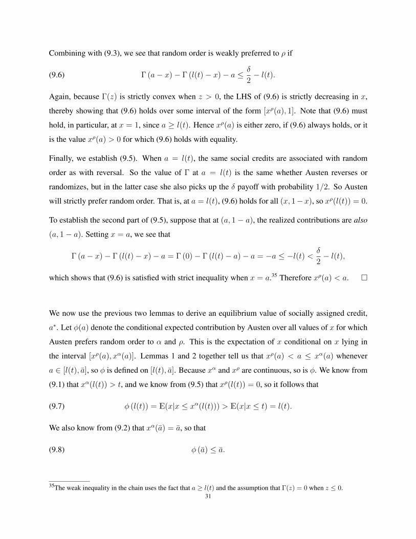
We now use the previous two lemmas to derive an equilibrium value of socially assigned credit,

a∗. Let φ(a) denote the conditional expected contribution by Austen over all values of x for which

Austen prefers random order to α and ρ. This is the expectation of x conditional on x lying in

the interval [xρ(a), xα(a)]. Lemmas 1 and 2 together tell us that xρ(a) < a ≤ xα(a) whenever

a ∈ [l(t), a], so φ is defined on [l(t), a]. Because xα and xρ are continuous, so is φ. We know from

(9.1) that xα(l(t)) > t, and we know from (9.5) that xρ(l(t)) = 0, so it follows that

(9.7) φ (l(t)) = E(x|x ≤ xα(l(t))) > E(x|x ≤ t) = l(t).

We also know from (9.2) that xα(a) = a, so that

(9.8) φ (a) ≤ a.

35The weak inequality in the chain uses the fact that a ≥ l(t) and the assumption that Γ(z) = 0 when z ≤ 0.31

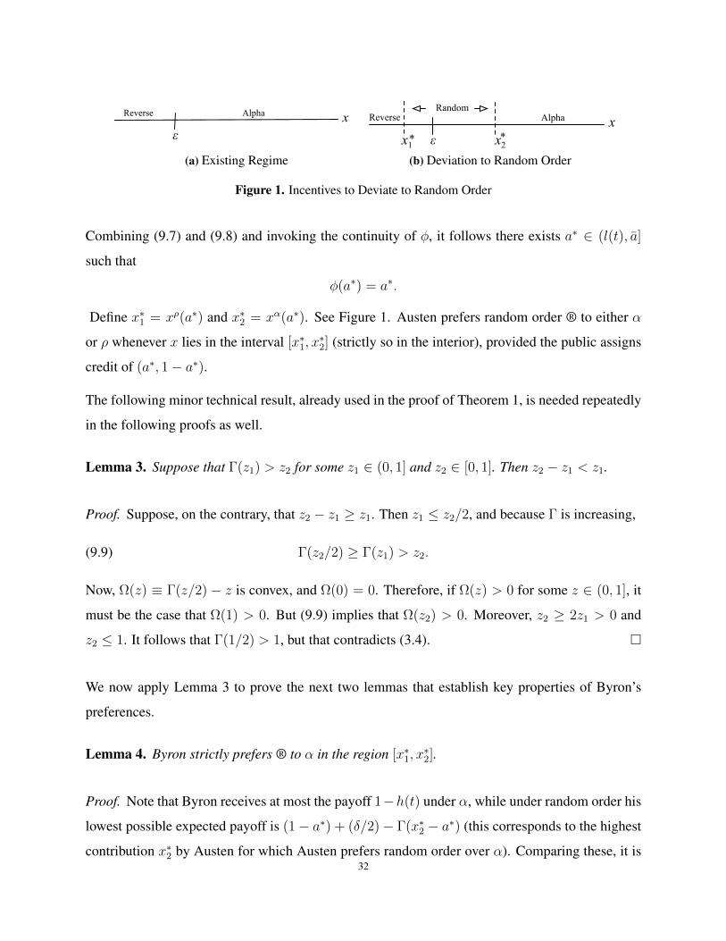
xε

Reverse Alpha

(a) Existing Regime

xε

Reverse Alpha

x1

Random

x2**

(b) Deviation to Random Order

Figure 1. Incentives to Deviate to Random Order

Combining (9.7) and (9.8) and invoking the continuity of φ, it follows there exists a∗ ∈ (l(t), a]

such that

φ(a∗) = a∗.

Define x∗1 = xρ(a∗) and x∗2 = xα(a∗). See Figure 1. Austen prefers random order ® to either α

or ρ whenever x lies in the interval [x∗1, x∗2] (strictly so in the interior), provided the public assigns

credit of (a∗, 1− a∗).

The following minor technical result, already used in the proof of Theorem 1, is needed repeatedly

in the following proofs as well.

Lemma 3. Suppose that Γ(z1) > z2 for some z1 ∈ (0, 1] and z2 ∈ [0, 1]. Then z2 − z1 < z1.

Proof. Suppose, on the contrary, that z2 − z1 ≥ z1. Then z1 ≤ z2/2, and because Γ is increasing,

(9.9) Γ(z2/2) ≥ Γ(z1) > z2.

Now, Ω(z) ≡ Γ(z/2)− z is convex, and Ω(0) = 0. Therefore, if Ω(z) > 0 for some z ∈ (0, 1], it

must be the case that Ω(1) > 0. But (9.9) implies that Ω(z2) > 0. Moreover, z2 ≥ 2z1 > 0 and

z2 ≤ 1. It follows that Γ(1/2) > 1, but that contradicts (3.4).

We now apply Lemma 3 to prove the next two lemmas that establish key properties of Byron’s

preferences.

Lemma 4. Byron strictly prefers ® to α in the region [x∗1, x∗2].

Proof. Note that Byron receives at most the payoff 1−h(t) under α, while under random order his

lowest possible expected payoff is (1− a∗) + (δ/2)− Γ(x∗2 − a∗) (this corresponds to the highest

contribution x∗2 by Austen for which Austen prefers random order over α). Comparing these, it is32

sufficient to show that

(9.10)δ

2+ (h(t)− a∗) > Γ(x∗2 − a∗).

Recall that Austen herself is indifferent over the two options at x∗2, so that

δ + h(t)− Γ (h(t)− x∗2) =δ

2+ a∗ − Γ(a∗ − x∗2) =

δ

2+ a∗,

(where the second equality comes from x∗2 = xα(a∗) ≥ a∗ by (9.2)). Transposing terms,

(9.11)δ

2+ [h(t)− a∗] = Γ (h(t)− x∗2) .

Define z1 ≡ h(t) − x∗2 and z2 ≡ h(t) − a∗. Since a∗ ≤ a < h(t) and (9.11) holds, the conditions

of Lemma 3 are met. It follows that x∗2 − a∗ < h(t) − x∗2. Combining this inequality with (9.11)

and recalling that Γ is increasing, we obtain (9.10).

Lemma 5. Byron strictly prefers ρ to ® when x < x∗1.

Proof. Under random order, Byron’s payoff is (1 − a∗) + (δ/2), there being no additional loss

because x < x∗1 < a∗. Under ρ, Byron’s lowest payoff occurs when x = x∗1, and it is given by

[1− l(t)] + δ − Γ(x∗1 − l(t)). So it is sufficient to show that

(9.12) a∗ − l(t) +δ

2> Γ(x∗1 − l(t)).

Because x < x∗1, we have x∗1 > 0, so that Austen is indifferent between ρ and ® at x∗1. Therefore

a∗ − l(t) +δ

2= Γ(a∗ − x∗1)− Γ(l(t)− x∗1).

Because a∗ > l(t), (9.12) is trivially true when x∗1 ≤ l(t). So we suppose that x∗1 > l(t), in which

case the above equality can be written as

(9.13) a∗ − l(t) +δ

2= Γ(a∗ − x∗1).

Define z1 ≡ a∗ − x∗1 and z2 ≡ a∗ − l(t). Since a∗ ≥ x∗1 ≥ l(t) and (9.13) holds, the conditions of

Lemma 3 are met. It follows that a∗ − x∗1 > x∗1 − l(t). Combining this inequality with (9.13) and

recalling that Γ is increasing, we obtain (9.12). 33

We can now complete the proof of the theorem. First we show that in the zone (x∗1, x∗2), ® is

an equilibrium outcome. Recall that ® is Austen’s favorite outcome in this range. By Lemma

4, Byron strictly prefers random order in this range to alphabetical order. Therefore ® strictly

Pareto-dominates the default and is not strictly Pareto-dominated itself, so it is a rational deviation

for all types in (x∗1, x∗2), by [I] and [II] of Section 3.6. (The zero probability endpoint x = x∗ can

be attached to either ® or ρ, and a similar assertion holds for x = x∗2.) Next, for x > x∗2, Austen

strictly prefers the default α to ®, so ® cannot be a rational deviation, by [I] of Section 3.6. For

x < x∗1, Austen strictly prefers ρ to ® by the construction of x∗1, and Byron does too, by Lemma 5.

Therefore ρ strictly Pareto dominates ®, which means that the latter cannot be a rational deviation,

by [II] of Section 3.6. We have therefore established that Et is rationally disrupted by random

order.

Proof of Theorem 3. We begin by setting up a particular random order convention (t∗, µ∗), and

then show it is an equilibrium. To this end, define for any m ∈ [0, 1] and t ∈ [0,m],

(9.14) ΨA(t,m) ≡ [m− l(t)] +δ

2− Γ(m− t),

and for any µ ∈ [m, 1],

(9.15) ΨB(µ,m) ≡ [h(µ)−m] +δ

2− Γ(µ−m).

First consider the general case in which f satisfies (6.1). The following lemma helps to obtain the

equilibrium socially assigned credit, m∗.

Lemma 6. Assume that (6.1) holds. Then whenever ΨA(t,m) ≤ 0, ΨA(t,m) > ΨA(t′,m) for all

t′ < t, and whenever ΨB(µ,m) ≤ 0, ΨB(µ,m) > ΨB(µ′,m) for all µ′ > µ.

Proof. Suppose that ΨA(t,m) ≤ 0. Pick t′ < t. Then

ΨA(t,m)−ΨA(t′,m) = [Γ(m− t′)− Γ(m− t)]− [l(t)− l(t′)]

≥ Γ′(m− t)(t− t′)− [l(t)− l(t′)]

≥ GΓ(m− t)(t− t′)

m− t− [l(t)− l(t′)]

≥ GΓ(m− t)(t− t′)

m− t−G(t− t′) > 0,

34

where the first inequality uses the convexity of Γ, the second inequality uses (6.1), and the very

last strict inequality uses the fact that ΨA(t,m) ≤ 0, so that Γ(m − t) > m − l(t) > m − t. The

proof for ΨB uses an entirely analogous argument.

Lemma 6 and the fact that ΨA(m,m) > 0 imply that for each m ∈ [0, 1], either ΨA(t,m) > 0 for

all t ∈ [0,m], or there is a unique value of t — call it t(m) — at which ΨA(t(m),m) = 0. In the

former case, set t(m) = 0 to complete the definition of this function t, where t(m) < m for all

m ∈ [0, 1]. In an analogous way, define a function µ, by µ(m) = 1 if ΨB(µ,m) > 0 for all µ ∈

[m, 1], or otherwise as the unique solution to ΨB(µ,m) = 0, so that µ(m) > m, for all m ∈ [0, 1].

Now define a mapping ζ as the conditional expectation ζ(m) = E(x|x ∈ [t(m), µ(m)]). Clearly,

ζ is continuous, and so has a fixed point. Pick any such fixed point; call it m∗ and fix it for the rest

of this proof. Define (t∗, µ∗) ≡ (t(m∗), µ(m∗)). This generates a random-order convention with

the following properties:

(i) 0 ≤ t∗ < m∗ < µ∗ ≤ 1; in particular, the randomization zone is always non-empty.

(ii) If t∗ > 0, then ΨA(t,m∗) < 0 when t < t∗ and ΨA(t,m∗) > 0 when t > t∗, where

ΨA(t∗,m∗) = 0 , with analogous properties for µ∗ and ΨB.

We claim that either at least one of the exception zones is nonempty. Suppose, on the contrary, that

t∗ = 0 and µ∗ = 1. Then m∗ = mA, and so ΨA(0,m∗) = mA + δ2− Γ(mA) ≥ 0, because t∗ = 0.

But this contradicts (3.3).

In the particular case where f is symmetric, (6.1) need not hold. Set m = 1/2, and note that

ΨA(1/2, 1/2) = 1/2 − l(1/2) + δ/2 > 0 but ΨA(0, 1/2) = 1/2 + δ/2 − Γ(1/2) < 0 by (3.4).

Hence there exists t∗ > 0 such that ΨA(t∗, 1/2) = 0. Set µ∗ = 1 − t∗ < 1. The symmetry here

implies that ΨB(µ∗, 1/2) = 0 and that m∗ ≡ E(x|x ∈ [t∗, µ∗]) = E(x|x ∈ [t∗, 1 − t∗) = 1/2 so

(t∗, 1− t∗) is our convention for the symmetric case, with all zones nontrivial.

We claim that any such solution described above — the fixed point for the non-symmetric case and

the symmetric convention for the symmetric case — is an equilibrium random-order convention.

To prove the claim, consider first the range 0 ≤ x < t∗, presuming this range is non-empty. We

show that in this range, Austen strictly prefers ρ to ®, while Byron strictly prefers ρ to either ® or

α; the latter being only relevant when used by the convention; that is, when µ∗ < 1.35

Begin with the claim for Austen. Observe that ρ yields Austen l(t∗)−Γ(l(t∗)−x), while ® yields

Austen m∗ + δ/2− Γ(m∗ − x). The difference between the latter and the former is given by

Λ ≡[m∗ +

δ

2− Γ(m∗ − x)

]− [l(t∗)− Γ(l(t∗)− x)] .

If x ≥ l(t∗), then Γ(l(t∗)− x) = 0 and so it is immediate that

Λ = [m∗ − l(t∗)] +δ

2− Γ(m∗ − x) < [m∗ − l(t∗)] +

δ

2− Γ(m∗ − t∗) = ΨA(t∗,m∗) = 0,

where the last equality follows from the definition of t∗ and the fact that t∗ > 0 in this case.

If x < l(t∗), then by the strict convexity of Γ (when positive), we see that Γ(m∗−x)−Γ(l(t∗)−x) >

Γ(m∗ − t∗)− Γ(l(t∗)− t∗) = Γ(m∗ − t∗), so that

Λ ≡ [m∗ − l(t∗)] +δ

2− [Γ(m∗ − x)− Γ(l(t∗)− x)] < ΨA(t∗,m∗) = 0.

In short, Λ < 0 whenever x < t∗, establishing the claim for Austen.

Turning now to Byron’s preferences in the range x < t∗, we first show that Byron strictly prefers ρ

to ®. Byron’s lowest payoff under ρ occurs when x = t∗; it is 1− l(t∗) + δ− Γ(t∗− l(t∗)). Under

®, his payoff is (1 −m∗) + (δ/2) − Γ(x −m∗), which is bounded above by (1 −m∗) + (δ/2).

Consequently, it suffices to show that

(9.16) [m∗ − l(t∗)] +δ

2> Γ(t∗ − l(t∗)).

Now, given that t∗ > 0, we know that

(9.17) ΨA(t∗,m∗) = [m∗ − l(t∗)] +δ

2− Γ(m∗ − t∗) = 0,

Define z1 ≡ m∗ − t∗ and z2 ≡ m∗ − l(t∗). Since m∗ ≥ t∗ ≥ l(t) and (9.17) holds, the conditions

of Lemma 3 are met. It follows that m∗ − t∗ > t∗ − l(t∗). Combining this inequality with (9.17)

and recalling that Γ is increasing, we obtain (9.16).

To complete the proof of the claim when x < t∗, we show that Byron strictly prefers ρ to α. For

ρ yields Byron a payoff of 1− l(t∗) + δ − Γ(x− l(t∗)), whereas α yields at most 1− h(µ∗). The

36

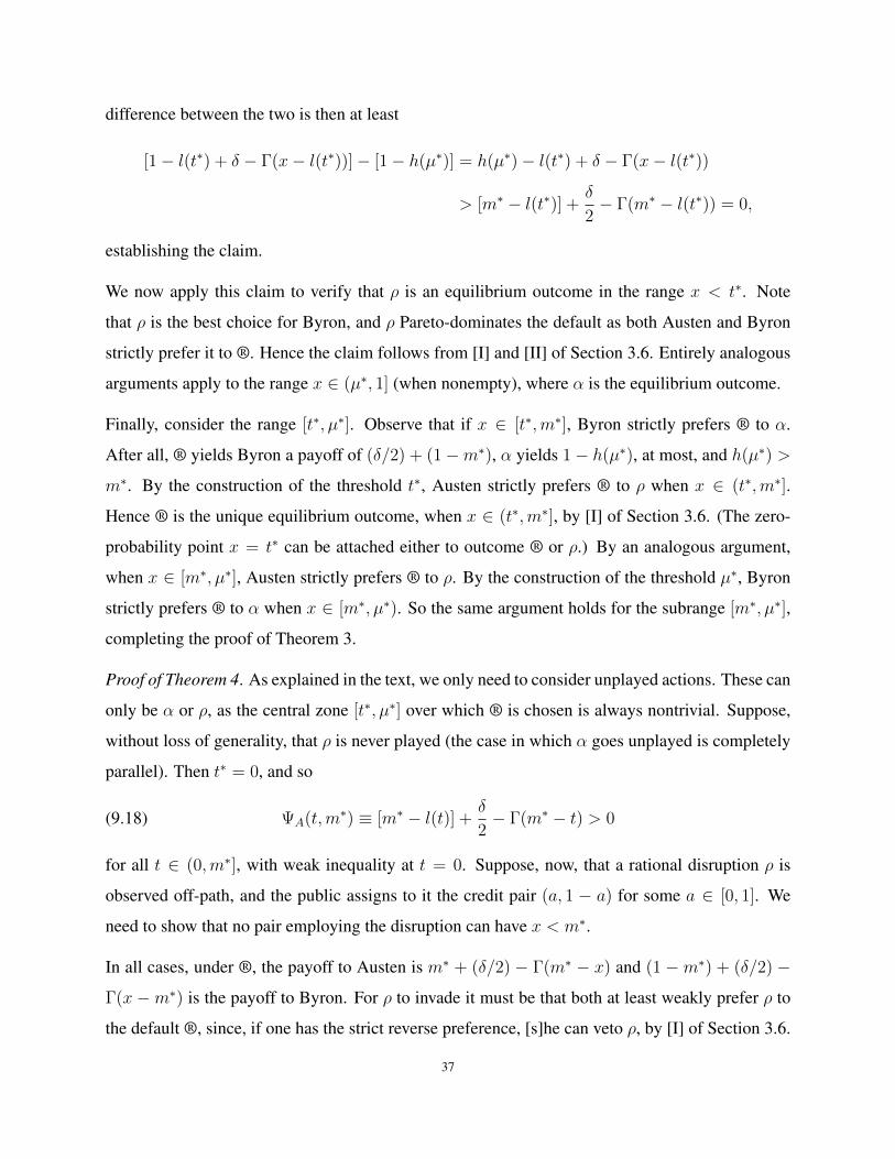
difference between the two is then at least

[1− l(t∗) + δ − Γ(x− l(t∗))]− [1− h(µ∗)] = h(µ∗)− l(t∗) + δ − Γ(x− l(t∗))

> [m∗ − l(t∗)] +δ

2− Γ(m∗ − l(t∗)) = 0,

establishing the claim.

We now apply this claim to verify that ρ is an equilibrium outcome in the range x < t∗. Note

that ρ is the best choice for Byron, and ρ Pareto-dominates the default as both Austen and Byron

strictly prefer it to ®. Hence the claim follows from [I] and [II] of Section 3.6. Entirely analogous

arguments apply to the range x ∈ (µ∗, 1] (when nonempty), where α is the equilibrium outcome.

Finally, consider the range [t∗, µ∗]. Observe that if x ∈ [t∗,m∗], Byron strictly prefers ® to α.

After all, ® yields Byron a payoff of (δ/2) + (1−m∗), α yields 1− h(µ∗), at most, and h(µ∗) >

m∗. By the construction of the threshold t∗, Austen strictly prefers ® to ρ when x ∈ (t∗,m∗].

Hence ® is the unique equilibrium outcome, when x ∈ (t∗,m∗], by [I] of Section 3.6. (The zero-

probability point x = t∗ can be attached either to outcome ® or ρ.) By an analogous argument,

when x ∈ [m∗, µ∗], Austen strictly prefers ® to ρ. By the construction of the threshold µ∗, Byron

strictly prefers ® to α when x ∈ [m∗, µ∗). So the same argument holds for the subrange [m∗, µ∗],

completing the proof of Theorem 3.

Proof of Theorem 4. As explained in the text, we only need to consider unplayed actions. These can

only be α or ρ, as the central zone [t∗, µ∗] over which ® is chosen is always nontrivial. Suppose,

without loss of generality, that ρ is never played (the case in which α goes unplayed is completely

parallel). Then t∗ = 0, and so

(9.18) ΨA(t,m∗) ≡ [m∗ − l(t)] +δ

2− Γ(m∗ − t) > 0

for all t ∈ (0,m∗], with weak inequality at t = 0. Suppose, now, that a rational disruption ρ is

observed off-path, and the public assigns to it the credit pair (a, 1 − a) for some a ∈ [0, 1]. We

need to show that no pair employing the disruption can have x < m∗.

In all cases, under ®, the payoff to Austen is m∗ + (δ/2) − Γ(m∗ − x) and (1 −m∗) + (δ/2) −

Γ(x −m∗) is the payoff to Byron. For ρ to invade it must be that both at least weakly prefer ρ to

the default ®, since, if one has the strict reverse preference, [s]he can veto ρ, by [I] of Section 3.6.

37

We must therefore have

a−Γ(a−x) ≥ m∗+(δ/2)−Γ(m∗−x) and (1−a)+δ−Γ(x−a) ≥ (1−m∗)+(δ/2)−Γ(x−m∗).

Combining these two inequalities, we have

(9.19) Γ(m∗ − x)− Γ(a− x) ≥ m∗ +δ

2− a ≥ Γ(x− a)− Γ(x−m∗).

Suppose first that a ≤ m∗. If x ≥ m∗, the left-hand side of (9.19) must be zero, while the middle

term is strictly positive, given that m∗ ≥ a, which is a contradiction. Therefore no pair with

x ≥ m∗ can deviate from ® to ρ. No pair playing α would want to deviate to ρ either. For such

a pair, x ≥ µ∗ > m∗, and each co-author weakly prefers α to ®, and even ® cannot be weakly

improved upon for both parties when x ≥ m∗. Hence it must be that x < m∗, if a ≤ m∗.

Suppose then that (9.19) holds for a nontrivial set of x ≥ 0, and let z ∈ (0,m∗] be the supremum

of the values of x for which (9.19) holds. By the convexity of Γ, it is easy to see that the LHS of

(9.19) is nonincreasing in x, while the RHS is nondecreasing. It follows that the set of deviants is

given by the set [0, z]. By rationality of disruptions, it must be that

(9.20) a = E(x|x ≤ z) = l(z).

In particular, z > a, so Γ(a− z) = 0. Therefore (9.19) implies

Γ(m∗ − z) ≥ m∗ +δ

2− a.

Using (9.20), we have

(9.21) Γ(m∗ − z) ≥ m∗ + (δ/2)− l(z),

but (9.21) and z > 0 contradict (9.18). Hence there can be no nontrivial disruption when a ≤ m∗.

This leaves the possibility that a > m∗. It cannot be that a ∈ (m∗,m∗ + δ/2). For there has to be

some pair with x ≥ a who would like to deviate. But for any x ≥ a, the LHS of (9.19) is zero,

while the middle term is positive, a contradiction. Therefore, a ≥ m∗ + δ/2. Now the lowest x

that might deviate is bounded below by m∗, for if x < m∗, then the LHS of (9.19) is negative, the

middle term is non-positive, and the RHS is zero, a contradiction.

38

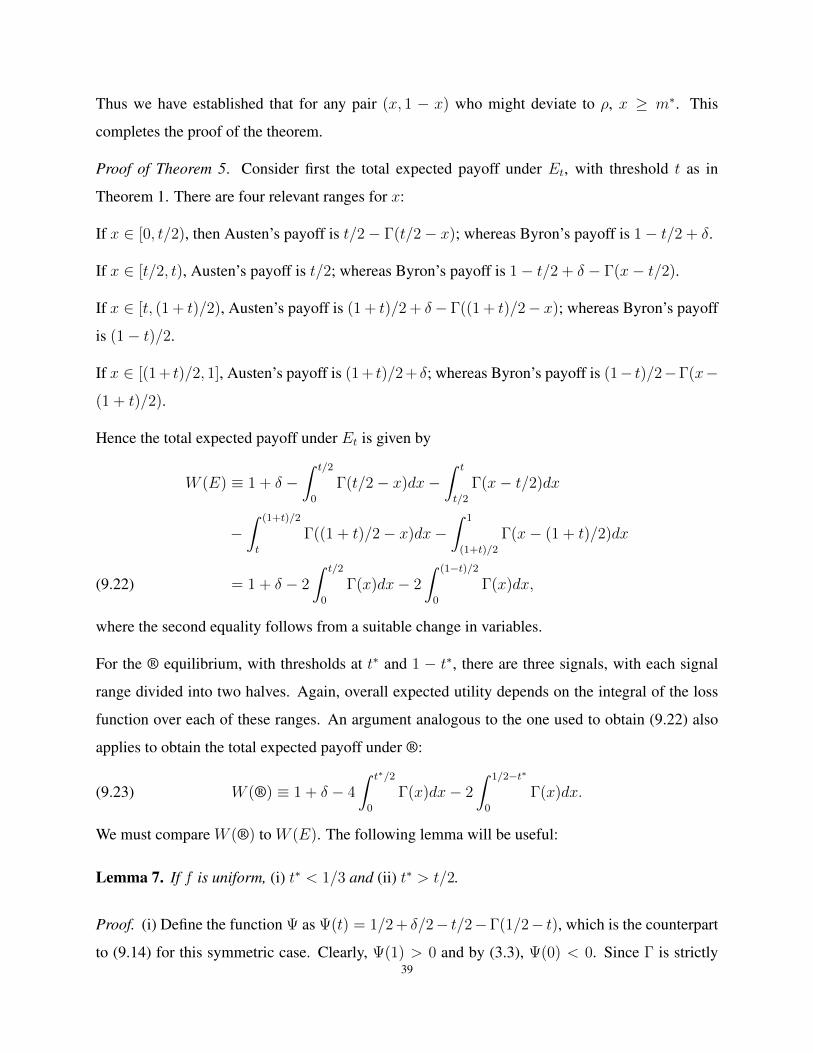
Thus we have established that for any pair (x, 1 − x) who might deviate to ρ, x ≥ m∗. This

completes the proof of the theorem.

Proof of Theorem 5. Consider first the total expected payoff under Et, with threshold t as in

Theorem 1. There are four relevant ranges for x:

If x ∈ [0, t/2), then Austen’s payoff is t/2− Γ(t/2− x); whereas Byron’s payoff is 1− t/2 + δ.

If x ∈ [t/2, t), Austen’s payoff is t/2; whereas Byron’s payoff is 1− t/2 + δ − Γ(x− t/2).

If x ∈ [t, (1 + t)/2), Austen’s payoff is (1 + t)/2 + δ− Γ((1 + t)/2− x); whereas Byron’s payoff

is (1− t)/2.

If x ∈ [(1 + t)/2, 1], Austen’s payoff is (1 + t)/2 + δ; whereas Byron’s payoff is (1− t)/2−Γ(x−

(1 + t)/2).

Hence the total expected payoff under Et is given by

W (E) ≡ 1 + δ −∫ t/2

0

Γ(t/2− x)dx−∫ t

t/2

Γ(x− t/2)dx

−∫ (1+t)/2

t

Γ((1 + t)/2− x)dx−∫ 1

(1+t)/2

Γ(x− (1 + t)/2)dx

= 1 + δ − 2

∫ t/2

0

Γ(x)dx− 2

∫ (1−t)/2

0

Γ(x)dx,(9.22)

where the second equality follows from a suitable change in variables.

For the ® equilibrium, with thresholds at t∗ and 1 − t∗, there are three signals, with each signal

range divided into two halves. Again, overall expected utility depends on the integral of the loss

function over each of these ranges. An argument analogous to the one used to obtain (9.22) also

applies to obtain the total expected payoff under ®:

(9.23) W (®) ≡ 1 + δ − 4

∫ t∗/2

0

Γ(x)dx− 2

∫ 1/2−t∗

0

Γ(x)dx.

We must compare W (®) to W (E). The following lemma will be useful:

Lemma 7. If f is uniform, (i) t∗ < 1/3 and (ii) t∗ > t/2.

Proof. (i) Define the function Ψ as Ψ(t) = 1/2 + δ/2− t/2−Γ(1/2− t), which is the counterpart

to (9.14) for this symmetric case. Clearly, Ψ(1) > 0 and by (3.3), Ψ(0) < 0. Since Γ is strictly39

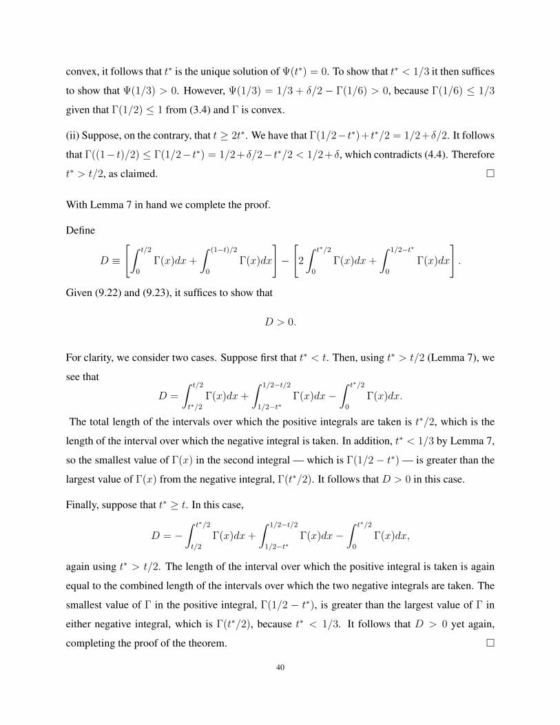
convex, it follows that t∗ is the unique solution of Ψ(t∗) = 0. To show that t∗ < 1/3 it then suffices

to show that Ψ(1/3) > 0. However, Ψ(1/3) = 1/3 + δ/2 − Γ(1/6) > 0, because Γ(1/6) ≤ 1/3

given that Γ(1/2) ≤ 1 from (3.4) and Γ is convex.

(ii) Suppose, on the contrary, that t ≥ 2t∗. We have that Γ(1/2− t∗)+ t∗/2 = 1/2+δ/2. It follows

that Γ((1− t)/2) ≤ Γ(1/2− t∗) = 1/2+δ/2− t∗/2 < 1/2+δ, which contradicts (4.4). Therefore

t∗ > t/2, as claimed.

With Lemma 7 in hand we complete the proof.

Define

D ≡

[∫ t/2

0

Γ(x)dx+

∫ (1−t)/2

0

Γ(x)dx

]−

[2

∫ t∗/2

0

Γ(x)dx+

∫ 1/2−t∗

0

Γ(x)dx

].

Given (9.22) and (9.23), it suffices to show that

D > 0.

For clarity, we consider two cases. Suppose first that t∗ < t. Then, using t∗ > t/2 (Lemma 7), we

see that

D =

∫ t/2

t∗/2

Γ(x)dx+

∫ 1/2−t/2

1/2−t∗Γ(x)dx−

∫ t∗/2

0

Γ(x)dx.

The total length of the intervals over which the positive integrals are taken is t∗/2, which is the

length of the interval over which the negative integral is taken. In addition, t∗ < 1/3 by Lemma 7,

so the smallest value of Γ(x) in the second integral — which is Γ(1/2− t∗) — is greater than the

largest value of Γ(x) from the negative integral, Γ(t∗/2). It follows that D > 0 in this case.

Finally, suppose that t∗ ≥ t. In this case,

D = −∫ t∗/2

t/2

Γ(x)dx+

∫ 1/2−t/2

1/2−t∗Γ(x)dx−

∫ t∗/2

0

Γ(x)dx,

again using t∗ > t/2. The length of the interval over which the positive integral is taken is again

equal to the combined length of the intervals over which the two negative integrals are taken. The

smallest value of Γ in the positive integral, Γ(1/2 − t∗), is greater than the largest value of Γ in

either negative integral, which is Γ(t∗/2), because t∗ < 1/3. It follows that D > 0 yet again,

completing the proof of the theorem.

40