cesifo, a munich-based, globe-spanning economic research ......venice summer institute 2014 ... the...

Venice Summer Institute 2014

REFORMING THE PUBLIC SECTOR

Organiser: Apostolis Philippopoulos

Workshop to be held on 25 – 26 July 2014 on the island of San Servolo in the Bay of Venice, Italy

HAIRCUT SIZE, HAIRCUT TYPE AND THE

PROBABILITY OF SERIAL SOVEREIGN DEBT

RESTRUCTURINGS

Christoph Schroeder CESifo GmbH • Poschingerstr. 5 • 81679 Munich, Germany

Tel.: +49 (0) 89 92 24 - 1410 • Fax: +49 (0) 89 92 24 - 1409

E-Mail: [email protected] • www.cesifo.org/venice

July 2014

CESifo, a Munich-based, globe-spanning economic research and policy advice institution

Venice Summer Institute

Haircut Size, Haircut Type and the Probability of

Serial Sovereign Debt Restructurings

Christoph Schröder* (ZEW Mannheim)

First Draft: February 2014

This Draft: June 2014

Work in Progress Do not cite without author’s permission

Abstract: This paper complements the empirical literature on sovereign debt restructurings by

analyzing potential impediments of the probability of (near-term) follow-up restructur-

ings after a restructuring has taken place. I look for these impediments in the restructur-

ings themselves by asking whether there are certain features to debt renegotiation pro-

cesses and outcomes that hamper serial restructurings. The probability of follow-up re-

structurings is estimated by means of survival models using a unique dataset that has

kindly been provided by Cruces and Trebesch (2013). I find that more comprehensive

debt remissions decrease the probability of serial restructurings significantly. Moreover,

outright face value haircuts reduce the probability of serial restructurings more strongly

than reductions in net present value due to maturity extensions and/or interest rate

reductions, which seems to contradict basic economic theory.

JEL Classification Code: H63, N20 Keywords: serial restructurings, sovereign debt restructuring

* Corresponding author:

Christoph Schröder, Department of Corporate Taxation and Public Finance, Centre for European Economic Research (ZEW), L7, 1, 68161 Mannheim, Germany, +49 (0)621 1235-390, [email protected]

1

1. Introduction

Even though Reinhart and Rogoff (2004, p. 53) acknowledge that “‘serial default’ is the

rule, not the exception”, there is still no study examining this phenomenon in greater

detail. Thus, to complement the literature, this paper provides an analysis of potential

impediments of serial sovereign debt restructurings. Most importantly, I look for these

impediments in sovereign restructurings themselves, asking whether there are certain

features to debt renegotiation outcomes that hamper (near-term) follow-up restructur-

ings. The results may be very important for answering the question of which measures

could be taken to reduce the probability of a country’s debt burden to become unsus-

tainable again (shortly) after the implementation of a debt restructuring. The paper’s

findings may also contribute to the discussion of a sovereign debt restructuring mecha-

nism for emerging markets (Krueger, 2000) or for European countries (Gianviti, Krue-

ger, Pisani-Ferry, Sapir, and von Hagen, 2010).

The sovereign debt literature has traditionally been concerned with the costs of defaults

and/or restructurings1 because these costs are often viewed to be the main reason why

sovereigns repay their debt. The idea is that, in the factual absence of legal enforcement

mechanisms, creditors of sovereigns generally cannot count ex ante on a debtor country

to repay its debt, if default or restructuring were non-costly alternatives (seminal paper

by Eaton and Gersovitz, 1981). The literature2 specifically discusses (i) direct credit

market costs like capital market exclusion or higher borrowing costs (Eaton and Gerso-

vitz, 1981; Gelos, Sandleris, and Sahay, 2011; Aguiar and Gopinath, 2006; Mendoza and

Yue, 2008; Borensztein and Panizza, 2009; Richmond and Diaz, 2009; Asonuma, 2010;

Yue, 2010; Cruces and Trebesch 2013), (ii) costs in the form of a trade decline or trade

sanctions (Rose, 2005; Martinez and Sandleris, 2011), (iii) a decline in economic output

(Tomz and Wright, 2007; Arellano, 2008; Mendoza and Yue, 2008; De Paoli, Hoggarth,

and Saporta, 2009; Levy-Yeyati and Panizza, 2011), (iv) adverse effects on the financial

and banking sector (Borensztein and Panizza, 2009; Levy-Yeyati, Martinez Peria, and

Schmukler, 2010; Gennaioli, Martin, and Rossi, Forthcoming), (v) negative spill-overs on

the private credit sector (Arteta and Hale, 2008; Das, Papaioannou, and Trebesch, 2012),

1 I distinguish between the terms “sovereign debt restructuring” and “sovereign default” because a default occurs when a country misses out on any interest or principal payment on the due date or beyond a pre-specified grace period while a restructuring can take place even in the absence of an outright default, i.e. pre-emptively, in order to prevent a probable default. 2 For a thorough review of the literature and an overview of stylized facts about sovereign debt restructurings in general, please see Das, Papaioannou and Trebesch (2012) as well as Panizza et al. (2009), Sturzenegger and Zettelmeyer (2006), as well as Tomz and Wright (2013).

2

(vi) adverse effects on FDI inflows (Fuentes and Saravia, 2010), and (vii) administrative

and negotiation costs (Das, Papaioannou, and Trebesch, 2012).

Even though many studies provide evidence for the general existence of negative conse-

quences of sovereign defaults and debt restructurings, the empirical literature is not

completely at one when it comes to the magnitude, the timing, and the duration of the

different costs considered. For example, some studies find that credit markets have a

rather short time memory when it comes to direct credit market costs like higher bor-

rowing costs and capital market exclusion (see e.g. Borensztein and Panizza, 2009, Gelos

et al., 2004). Nevertheless, at least for “final restructurings”3 Cruces and Trebesch

(2013) find that, when controlling for the sizes of haircuts, capital market exclusion can

take a long time and borrowing costs can be significantly higher following a restructur-

ing. Also Richmond and Diaz (2009) estimate the average duration of capital market ex-

clusion to be non-negligible, taking approximately six to eight years. Unfortunately,

these authors do not control for the restructuring history: They do not explicitly take

into account whether a country had been a serial defaulter or not, which potentially in-

fluences their reputation as good debtors and the resulting capital market sanctions sig-

nificantly.

In spite of all potential costs mentioned above, debt restructuring can be a well justified

measure for a country facing an unmanageable debt burden in order to regain long-term

debt sustainability. However, the lack of a reliable sovereign debt restructuring mecha-

nism creates uncertainty for both debtors and creditors and may hamper the enforce-

ment of necessary debt exchanges that could in fact restore debt sustainability. The IMF

(2013, p. 15) argues that “unsustainable debt situations often fester before they are re-

solved and, when restructurings do occur, they do not always restore sustainability and

market access in a durable manner, leading to repeated restructurings.” Generally, noth-

ing is gained if a country restructures its debt too late and to an extent that is insufficient

for regaining long(er) term debt sustainability. “[T]oo little and too late” (IMF, 2013, p.

7) restructurings likely have negative consequences for debtors, creditors and, depend-

ing on the relative importance of the country in question, for the international financial

system. Persistent unsustainable debt levels impede investment and growth in the debt-

or country, thereby reducing the value of creditors’ claims even further.

3 Cruces and Trebesch (2013) define final restructurings as restructurings that were not succeeded by another restructuring with commercial creditors within four years.

3

The confident assumption in this paper is that serial and apparently insufficient restruc-

turings are in sum more costly than a single deemed-to-satisfy restructuring because

they do not raise a country’s reputation of being a good borrower but likely destroy the

reputation even more. Additionally, the administrative costs as well as the economic

costs due to the uncertain outcome of debt renegotiations (in terms of debt sustainabil-

ity) have to be incurred over and over again. Fuentes and Saravia (2010) find that the

decrease of FDI inflows is even stronger for serial defaulters than for single defaulters.

The IMF (2013, pp. 23-24) states that “[s]ince a restructuring process is disruptive and

costly to the debtor’s perceived creditworthiness, it is not desirable to repeat it.”

Throughout this paper, I neglect the possibility that a country might restructure its debt

serially for strategic reasons. Even if single restructurings were “strategic” in nature, the

series is likely not to be. Such a strategy is highly precarious, bears high risks and uncer-

tainty, and is thus quite likely to be an exception to the rule.

The empirical literature on serial sovereign debt restructurings is unfortunately very

scarce if not non-existent. There are merely a few studies relying on basic descriptive

observations and case studies. One study by Moody’s (2012) touches upon the issue and

suggests that an initial debt exchange was followed by further exchanges when the ini-

tial debt exchange was not large enough in relation to a country’s total debt (even when

the haircut of the initial exchange was large). Das et al. (2012, p. 33) speculate on a simi-

lar reason. They argue that debt relief in restructurings with official creditors (i.e. within

the so-called Paris Club4) has been too low before the 1990s, thus triggering serial de-

faults more often during the 1970s/1980s. The IMF (2013, p. 1) highlights that debt re-

structurings “have often been too little and too late, thus failing to re-establish debt sus-

tainability and market access in a durable way”. It further makes a case for the avoid-

ance of outright default and promotes pre-emptive debt restructurings in the view of

serious liquidity or solvency problems because pre-emptive restructurings entail pre-

dictable cash flows (as opposed to defaults) which make the consequences for the econ-

omy more predictable, too. The IMF (2013) further argues that materialized defaults

may undermine a country’s capacity to re-access international private capital markets in

the medium term.

I test these partly intuitive statements statistically and econometrically by estimating so-

called survival models. Additionally, I explore whether outright cuts in face value have

4 “The Paris Club is an informal group of official creditors whose role is to find coordinated and sustainable solutions to the payment difficulties experienced by debtor countries.” See http://www.clubdeparis.org/

4

the same impeding effect on serial restructurings as maturity lengthening and the lower-

ing of interest payments that lead to an equally sized haircut in net present value. Eco-

nomic theory suggests that any reduction in net present value, no matter whether it is

effectuated by cuts in face value, maturity extension or a lower interest rate, should have

the same impact on a country’s debt sustainability. I also investigate which characteris-

tics of the affected debt and the outcomes of the negotiations are correlated with the

probability of a follow-up restructuring.

The main findings suggest that higher overall haircuts in net present value are indeed

associated with a lower probability of serial restructurings. Interestingly, cuts in face

value have a stronger negative impact on this probability than reductions in net present

value by the means of maturity extensions and/or interest rate reductions. This puzzling

finding challenges theoretical expectations.

The remainder of the paper is structured as follows. Section 2 describes the dataset used

and provides some stylized facts. Section 3 descriptively analyzes correlations between

restructuring characteristics and the probability of (near-term) follow-up restructur-

ings. Section 4 presents the estimation results of Cox (1972) proportional hazard models

and section 5 concludes.

2. Data

2.2. Data Source for Restructurings with Commercial Creditors

The main dataset I use covers all 180 sovereign debt restructurings with foreign com-

mercial creditors in 68 countries since 1970 and has kindly been provided by Cruces

and Trebesch (2013)5. They report sovereign debt restructurings of public or publicly

guaranteed debt with foreign private creditors. The authors focus on distressed debt

exchanges, which they define as restructurings of bonds or bank loans at less favorable

conditions than the original bond or bank loan. They restrict the sample to medium and

long-term debt restructurings. Short-term agreements like 90-day debt rollovers or the

upkeep of short-term credit lines (e.g. trade credit) are disregarded and agreements

with maturity extension of less than one year are excluded. Cases where short-term debt

is exchanged for debt with a maturity of more than one year are, in turn, included. Final-

ly, the dataset covers only restructurings that have actually been implemented.

5 The dataset is freely accessible online: https://sites.google.com/site/christophtrebesch/data

5

The value of the dataset does not only lie in the mere listing of all these restructurings

but especially in the provision of information on the characteristics of the restructur-

ings. Most importantly, Cruces and Trebesch (2013, p. 87) estimate the “wealth loss of

the average creditor participating in the exchange”, i.e. they estimate what is generally

called a haircut in net present value. The authors use two different haircut measures: the

“market haircut” and the, in their view better suited, “SZ haircut” according to the meth-

odology of Sturzenegger and Zettelmeyer (2006, 2008)6. The dataset also includes the

magnitude of the cut in the nominal value of the debt, which is zero in 123 of the 180

cases.

Furthermore, Cruces and Trebesch (2013) provide information on the absolute amount

of debt (in current US dollars) that had been affected as well as other important features

of debt contracts, the debt affected and negotiation outcomes. The features of the debt

contracts and the debt affected include information on whether the debt was in the form

of bonds or bank loans, whether all of the debt affected had already fallen due at the

time of debt renegotiations, whether the debt affected included previously restructured

debt, and whether short-term debt with a maturity of less than one year had also been

restructured such that the new maturity exceeded one year. The features of negotiation

outcomes include information on whether the restructuring deal was a buy-back deal

(i.e. a country buys back its debt at large discount), whether the restructuring deal was a

so-called Brady deal7 (i.e. loosely speaking an exchange of bank loans for partly collat-

eralized tradable bonds), whether the deal was “donor-funded or supported by bilateral

or multilateral money, e.g. via funds by International Development Association Debt Re-

duction Facility”, and whether the deal “include[d] the provision of new money or con-

certed lending” (Cruces and Trebesch, 2013, online Appendix A5, p. 39).

6 The traditional “market haircut” compares the present value of new debt contracts to the face value of the old debt contracts, whereas the “SZ haircut” is computed according to the methodology by Sturzenegger and Zet-telmeyer (2008) who evaluate old debt contracts in present value terms and discount both new and old debt in-struments at the same interest rate. See Sturzenegger and Zettelmeyer (2008) as well as Cruces and Trebesch (2013) for a discussion of the advantages and disadvantages of the two haircut concepts. 7 Brady deals featured the conversion of bank loans to a variety of new tradable bonds for mostly Latin Ameri-can countries. The new bonds were partly collateralized by U.S. Treasury 30-year zero-coupon bonds. The main advantage was the possibility for commercial banks to exchange their claims on developing countries into trada-ble debt instruments, which greatly reduced the concentration of risk on their balance sheets. Argentina, Brazil, Bulgaria, Costa Rica, Côte d'Ivoire, Dominican Republic, Ecuador, Jordan, Mexico, Morocco, Nigeria, Panama, Peru, Philippines, Poland, Uruguay, Venezuela and Vietnam deployed the Brady program, named after the U.S. Treasury Secretary Nicholas Brady.

6

2.2. Data Source for Paris Club Debt Restructurings

Although I focus on debt restructurings with commercial creditors in the descriptive and

econometric sections 3 and 4, I include the restructurings with official creditors (Paris

Club) in the subsection 2.3 on the stylized facts. This helps the reader to get a more

complete picture of the problem.

I gathered the available data on all Paris Club restructurings since 1950 from the Paris

Club’s website8 and double-checked this list of restructurings with that of Das et al.

(2012). Surprisingly, there are ten Paris Club Restructurings in their list which I cannot

find on the official Paris Club’s website. I work with those 421 restructurings of 86 coun-

tries since 1970 that I could find on the Paris Club’s website.

2.3. Some Stylized Facts about Serial Restructurings

When simply looking at the timing of sovereign debt restructurings, one can easily make

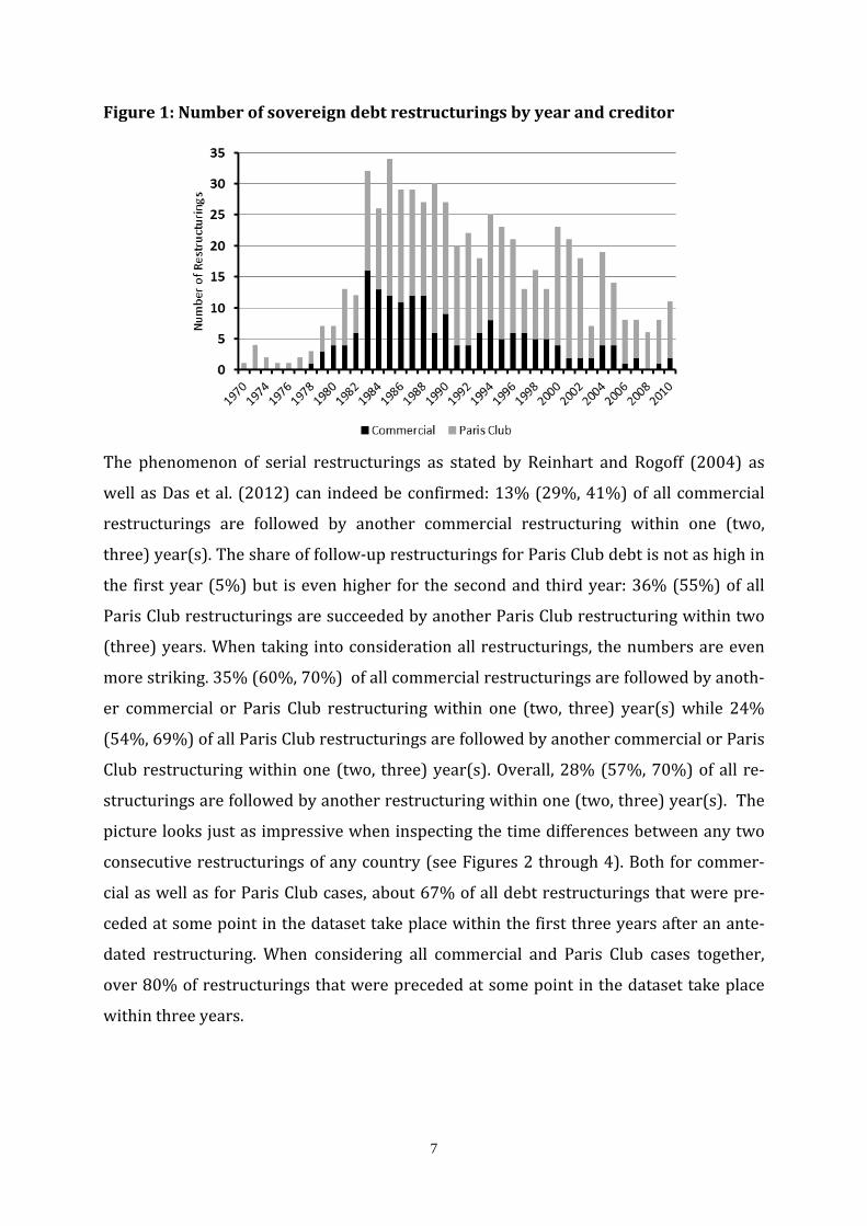
out restructuring clusters. Figure 19 shows a sharp increase in the number of restructur-

ings worldwide in the beginning of the 1980s and an overall peak in 1983. Especially the

number of commercial restructurings was highest during this decade and also peaked in

1983. While there were only four commercial restructurings in the 1970s (all of them in

the late 1970s) their number declined significantly starting in the late 1980s until 2010.

The trend looks similar for Paris Club restructurings, even though the volatility of the

number of restructurings per year was much higher. Das et al. (2012, p. 33) explain the

higher number and frequency of Paris Club restructurings (as opposed to commercial

restructurings) by the “Paris Club’s reluctance to grant debt relief” before the 1990s.

They hypothesize that “[t]his likely triggered a pattern of serial rescheduling with some

debtors.”

8 http://www.clubdeparis.org/ 9 A similar figure can be found in Das et al. (2012).

7

Figure 1: Number of sovereign debt restructurings by year and creditor

The phenomenon of serial restructurings as stated by Reinhart and Rogoff (2004) as

well as Das et al. (2012) can indeed be confirmed: 13% (29%, 41%) of all commercial

restructurings are followed by another commercial restructuring within one (two,

three) year(s). The share of follow-up restructurings for Paris Club debt is not as high in

the first year (5%) but is even higher for the second and third year: 36% (55%) of all

Paris Club restructurings are succeeded by another Paris Club restructuring within two

(three) years. When taking into consideration all restructurings, the numbers are even

more striking. 35% (60%, 70%) of all commercial restructurings are followed by anoth-

er commercial or Paris Club restructuring within one (two, three) year(s) while 24%

(54%, 69%) of all Paris Club restructurings are followed by another commercial or Paris

Club restructuring within one (two, three) year(s). Overall, 28% (57%, 70%) of all re-

structurings are followed by another restructuring within one (two, three) year(s). The

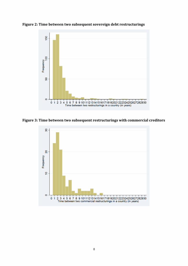
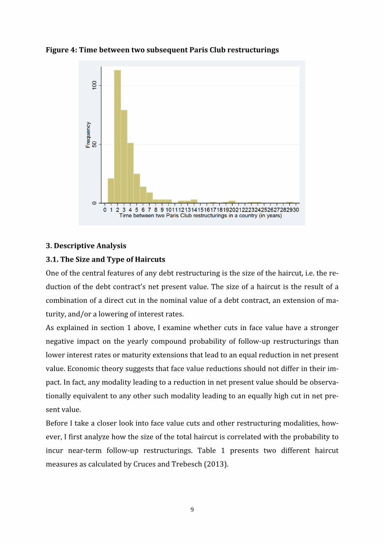
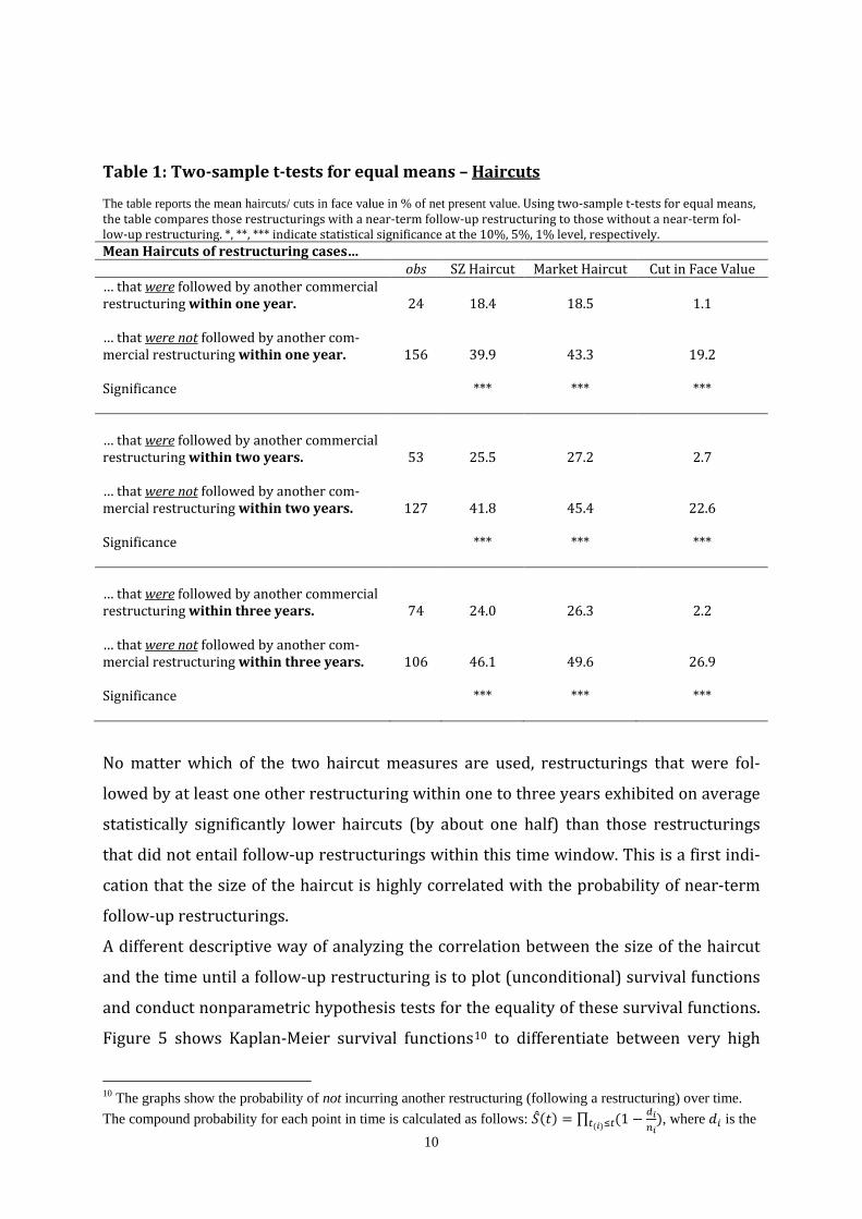
picture looks just as impressive when inspecting the time differences between any two

consecutive restructurings of any country (see Figures 2 through 4). Both for commer-

cial as well as for Paris Club cases, about 67% of all debt restructurings that were pre-

ceded at some point in the dataset take place within the first three years after an ante-

dated restructuring. When considering all commercial and Paris Club cases together,

over 80% of restructurings that were preceded at some point in the dataset take place

within three years.

8

Figure 2: Time between two subsequent sovereign debt restructurings

Figure 3: Time between two subsequent restructurings with commercial creditors

9

Figure 4: Time between two subsequent Paris Club restructurings

3. Descriptive Analysis

3.1. The Size and Type of Haircuts

One of the central features of any debt restructuring is the size of the haircut, i.e. the re-

duction of the debt contract’s net present value. The size of a haircut is the result of a

combination of a direct cut in the nominal value of a debt contract, an extension of ma-

turity, and/or a lowering of interest rates.

As explained in section 1 above, I examine whether cuts in face value have a stronger

negative impact on the yearly compound probability of follow-up restructurings than

lower interest rates or maturity extensions that lead to an equal reduction in net present

value. Economic theory suggests that face value reductions should not differ in their im-

pact. In fact, any modality leading to a reduction in net present value should be observa-

tionally equivalent to any other such modality leading to an equally high cut in net pre-

sent value.

Before I take a closer look into face value cuts and other restructuring modalities, how-

ever, I first analyze how the size of the total haircut is correlated with the probability to

incur near-term follow-up restructurings. Table 1 presents two different haircut

measures as calculated by Cruces and Trebesch (2013).

10

Table 1: Two-sample t-tests for equal means – Haircuts

The table reports the mean haircuts/ cuts in face value in % of net present value. Using two-sample t-tests for equal means, the table compares those restructurings with a near-term follow-up restructuring to those without a near-term fol-low-up restructuring. *, **, *** indicate statistical significance at the 10%, 5%, 1% level, respectively. Mean Haircuts of restructuring cases… obs SZ Haircut Market Haircut Cut in Face Value … that were followed by another commercial restructuring within one year. 24 18.4 18.5 1.1 … that were not followed by another com-mercial restructuring within one year. 156 39.9 43.3 19.2 Significance *** *** *** … that were followed by another commercial restructuring within two years. 53 25.5 27.2 2.7 … that were not followed by another com-mercial restructuring within two years. 127 41.8 45.4 22.6 Significance *** *** *** … that were followed by another commercial restructuring within three years. 74 24.0 26.3 2.2 … that were not followed by another com-mercial restructuring within three years. 106 46.1 49.6 26.9 Significance *** *** ***

No matter which of the two haircut measures are used, restructurings that were fol-

lowed by at least one other restructuring within one to three years exhibited on average

statistically significantly lower haircuts (by about one half) than those restructurings

that did not entail follow-up restructurings within this time window. This is a first indi-

cation that the size of the haircut is highly correlated with the probability of near-term

follow-up restructurings.

A different descriptive way of analyzing the correlation between the size of the haircut

and the time until a follow-up restructuring is to plot (unconditional) survival functions

and conduct nonparametric hypothesis tests for the equality of these survival functions.

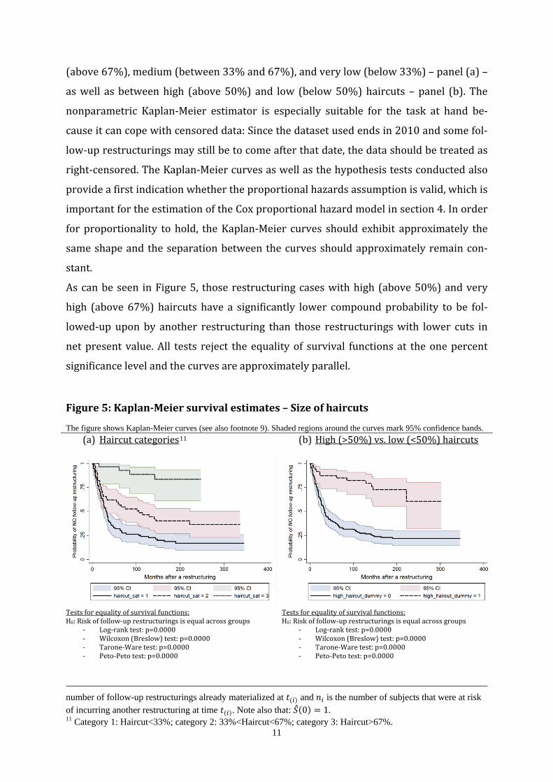
Figure 5 shows Kaplan-Meier survival functions10 to differentiate between very high

10 The graphs show the probability of not incurring another restructuring (following a restructuring) over time. The compound probability for each point in time is calculated as follows: �̂�(𝑡) = ∏ (1 − 𝑑𝑖

𝑛𝑖)𝑡(𝑖)≤𝑡 , where 𝑑𝑖 is the

11

(above 67%), medium (between 33% and 67%), and very low (below 33%) – panel (a) –

as well as between high (above 50%) and low (below 50%) haircuts – panel (b). The

nonparametric Kaplan-Meier estimator is especially suitable for the task at hand be-

cause it can cope with censored data: Since the dataset used ends in 2010 and some fol-

low-up restructurings may still be to come after that date, the data should be treated as

right-censored. The Kaplan-Meier curves as well as the hypothesis tests conducted also

provide a first indication whether the proportional hazards assumption is valid, which is

important for the estimation of the Cox proportional hazard model in section 4. In order

for proportionality to hold, the Kaplan-Meier curves should exhibit approximately the

same shape and the separation between the curves should approximately remain con-

stant.

As can be seen in Figure 5, those restructuring cases with high (above 50%) and very

high (above 67%) haircuts have a significantly lower compound probability to be fol-

lowed-up upon by another restructuring than those restructurings with lower cuts in

net present value. All tests reject the equality of survival functions at the one percent

significance level and the curves are approximately parallel.

Figure 5: Kaplan-Meier survival estimates – Size of haircuts

The figure shows Kaplan-Meier curves (see also footnote 9). Shaded regions around the curves mark 95% confidence bands. (a) Haircut categories11

Tests for equality of survival functions: H0: Risk of follow-up restructurings is equal across groups

- Log-rank test: p=0.0000 - Wilcoxon (Breslow) test: p=0.0000 - Tarone-Ware test: p=0.0000 - Peto-Peto test: p=0.0000

(b) High (>50%) vs. low (<50%) haircuts



number of follow-up restructurings already materialized at 𝑡(𝑖) and 𝑛𝑖 is the number of subjects that were at risk of incurring another restructuring at time 𝑡(𝑖). Note also that: �̂�(0) = 1. 11 Category 1: Haircut<33%; category 2: 33%<Haircut<67%; category 3: Haircut>67%.

12

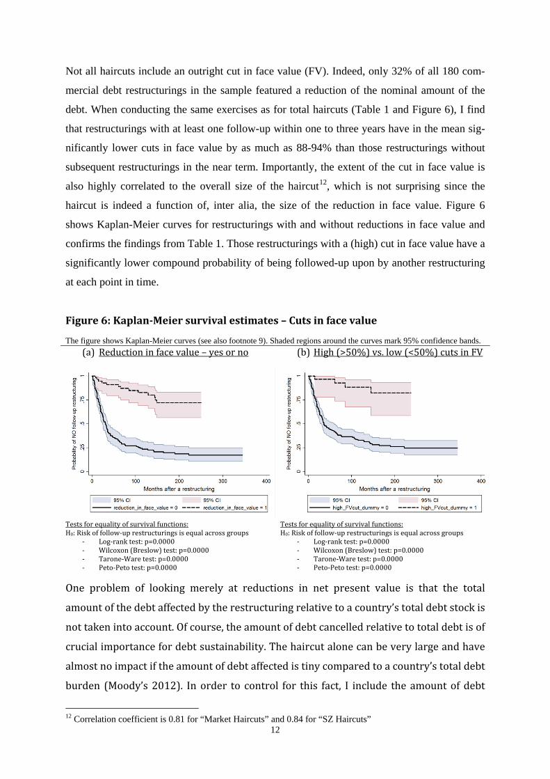
Not all haircuts include an outright cut in face value (FV). Indeed, only 32% of all 180 com-

mercial debt restructurings in the sample featured a reduction of the nominal amount of the

debt. When conducting the same exercises as for total haircuts (Table 1 and Figure 6), I find

that restructurings with at least one follow-up within one to three years have in the mean sig-

nificantly lower cuts in face value by as much as 88-94% than those restructurings without

subsequent restructurings in the near term. Importantly, the extent of the cut in face value is

also highly correlated to the overall size of the haircut12, which is not surprising since the

haircut is indeed a function of, inter alia, the size of the reduction in face value. Figure 6

shows Kaplan-Meier curves for restructurings with and without reductions in face value and

confirms the findings from Table 1. Those restructurings with a (high) cut in face value have a

significantly lower compound probability of being followed-up upon by another restructuring

at each point in time.

Figure 6: Kaplan-Meier survival estimates – Cuts in face value

The figure shows Kaplan-Meier curves (see also footnote 9). Shaded regions around the curves mark 95% confidence bands. (a) Reduction in face value – yes or no



(b) High (>50%) vs. low (<50%) cuts in FV



One problem of looking merely at reductions in net present value is that the total

amount of the debt affected by the restructuring relative to a country’s total debt stock is

not taken into account. Of course, the amount of debt cancelled relative to total debt is of

crucial importance for debt sustainability. The haircut alone can be very large and have

almost no impact if the amount of debt affected is tiny compared to a country’s total debt

burden (Moody’s 2012). In order to control for this fact, I include the amount of debt

12 Correlation coefficient is 0.81 for “Market Haircuts” and 0.84 for “SZ Haircuts”

13

affected by the restructuring relative to a country’s total debt stock as a control variable

in the estimations in section 5.

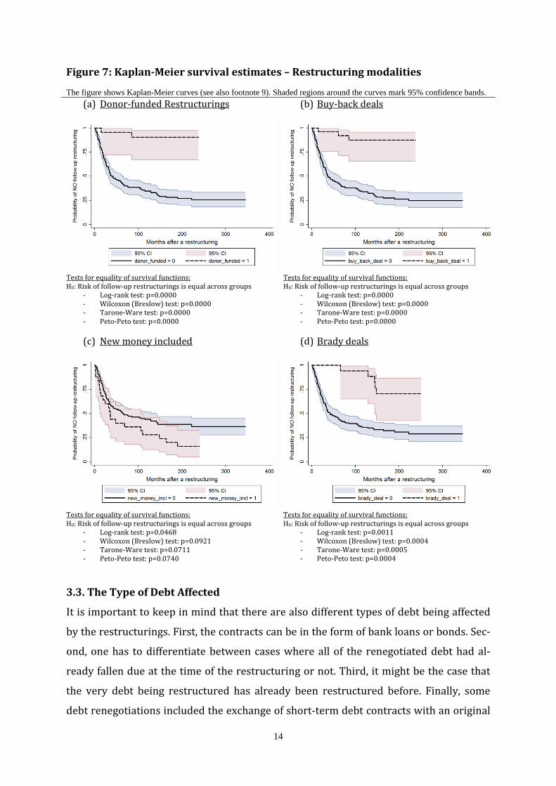
3.2. Other Modalities of Debt Restructurings

Of course, the size of a restructuring and the type of haircut is not the only outcome of

debt renegotiations that is potentially correlated with the probability of follow-up re-

structurings. Cruces and Trebesch (2013) also provide information on whether a re-

structuring has been donor funded, whether it comprised a buy-back of debt contracts,

whether the restructuring was a Brady deal (i.e. loosely speaking an exchange of bank

loans for partly collateralized tradable bonds) or whether it included the provision of

new money or concerted lending. Indeed, all of these features, except for the provision of

new money, are negatively and significantly correlated with the compound probability

of observing at least one follow-up restructuring (see Figure 7).

Donor funded restructurings (panel a) generally seem not to entail (many) near-term

follow-up restructurings but the causality is not clear at all. It might well be that donors

only provide funds to debtors, if they expect them to have a low probability of their debt

stock becoming unsustainable and having to restructure again in the future. Thus, we

cannot know whether donor funding just works well with respect to a lower probability

of serial restructurings or whether these restructuring cases were characterized by a

lower probability of serial default, to begin with.

The argument for buy-back deals (panel b) and restructurings that included the provi-

sion of new money (panel c) is similar. Countries which can afford to buy back their debt

contracts (even if they do so at a large discount) may anticipate a higher probability of

being sustainable afterwards. Oftentimes, donor funding and buying back debt even co-

incide, which makes the exogeniety assumption for these dummy variables with respect

to the probability of serial restructurings even more difficult to defend. Due to these po-

tential reverse causality problems, the baseline estimations in the econometric section

4.2 will not include these variables. Furthermore, I will check for robustness of overall

results by excluding these restructurings in section 4.3. This way, I can circumvent any

potential omission of variables that should actually necessarily be included in order to

control for particularities of these restructurings.

The exchange of bank loans for tradable Brady bonds in the 1980s also seems to have

worked quite well, when it comes to preventing near-term follow-up restructurings.

However, some of the countries had to restructure again 6 to 13 years later.

14

Figure 7: Kaplan-Meier survival estimates – Restructuring modalities

The figure shows Kaplan-Meier curves (see also footnote 9). Shaded regions around the curves mark 95% confidence bands. (a) Donor-funded Restructurings



(b) Buy-back deals



(c) New money included



(d) Brady deals



3.3. The Type of Debt Affected

It is important to keep in mind that there are also different types of debt being affected

by the restructurings. First, the contracts can be in the form of bank loans or bonds. Sec-

ond, one has to differentiate between cases where all of the renegotiated debt had al-

ready fallen due at the time of the restructuring or not. Third, it might be the case that

the very debt being restructured has already been restructured before. Finally, some

debt renegotiations included the exchange of short-term debt contracts with an original

15

maturity of at most one year for new debt instruments with a longer-term maturity ex-

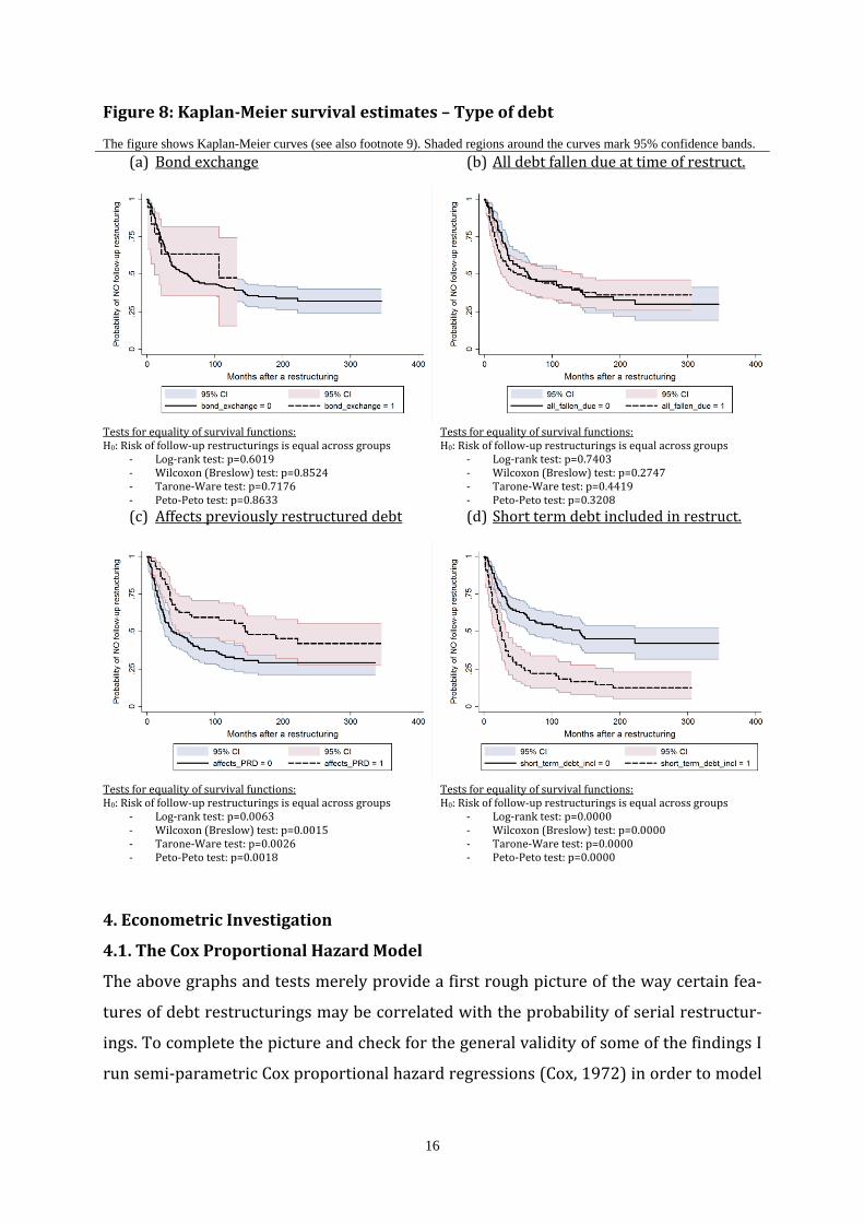
ceeding one year. When looking at the survival functions (Figure 8), only the facts that

previously restructured debt (PRD) has been renegotiated again (panel c) and that

short-term debt has been exchanged for longer-term debt (panel c) seem to be correlat-

ed with the compound probability of follow-up restructurings. Those cases where previ-

ously restructured debt has been restructured again, exhibit a statistically significant

lower probability of being followed by another restructuring at each point in time. This

may be the case because in these restructurings it was clear that the previous restruc-

turing had not been sufficient for the country to regain medium to long term debt sus-

tainability. These restructurings are by definition follow-up restructurings themselves.

Those restructurings where originally short-term debt was exchanged for longer-term

debt exhibit a higher compound probability of follow-up restructurings at each point in

time, which may initially be surprising. However, short-term debt being affected is a sign

of perceived liquidity problems (rather than real solvency problems). Exchanging short

to longer term debt is an attempt to reduce any acute liquidity pressure. Therefore it is

also not surprising that only two out of a total of 54 cases, where short-term debt had

been included, featured a (low) reduction in face value. The other 52 cases only com-

prised maturity lengthening and at best interest rate reductions. These cases may well

have developed to become real solvency problems, though. Thus, they are followed by

further restructurings with higher probability.

16

Figure 8: Kaplan-Meier survival estimates – Type of debt

The figure shows Kaplan-Meier curves (see also footnote 9). Shaded regions around the curves mark 95% confidence bands. (a) Bond exchange



(b) All debt fallen due at time of restruct.



(c) Affects previously restructured debt



(d) Short term debt included in restruct.



4. Econometric Investigation

4.1. The Cox Proportional Hazard Model

The above graphs and tests merely provide a first rough picture of the way certain fea-

tures of debt restructurings may be correlated with the probability of serial restructur-

ings. To complete the picture and check for the general validity of some of the findings I

run semi-parametric Cox proportional hazard regressions (Cox, 1972) in order to model

17

the simultaneous impact of certain debt renegotiation outcomes and debt characteristics

on the probability of a follow-up restructuring taking place at any point in time.

The Cox proportional hazard model allows estimating the hazard rate ℎ(𝑡) (i.e. the risk

of a follow-up restructuring to occur at a time 𝑡) and can be written as follows,

ℎ(𝑡) = ℎ0(𝑡) ∗ exp (𝛽1𝑋1 + 𝛽2𝑋2 + ⋯+ 𝛽𝑛𝑋𝑛) ,

where 𝑋1, … ,𝑋𝑛 denote the covariates and 𝛽1, … ,𝛽𝑛 are the corresponding coefficients.

The term ℎ0(𝑡) is the baseline hazard rate at time 𝑡 for all covariates being equal to zero

(similar to the constant term in simple linear regressions). The baseline hazard rate is

then shifted up or down by an order of proportionality when one of the covariates

changes.

The main advantage of the Cox proportional hazard model is the fact that the baseline

hazard function is left unparameterized, meaning that one does not have to assume a

specific functional form. This of course, can also be a disadvantage, since the proportion-

ality assumption must hold for the reduced form model to be correct. In addition to the

Kaplan-Meyer plots and the hypotheses tests for the equality of survival functions in

section 3 above, I also conduct post-estimation tests on the basis of Schoenfeld residuals

to check for the validity of this crucial assumption.

Another big advantage of the Cox model is that it can cope with left truncation and right

censoring, which is the case for the data at hand. Countries enter the dataset at different

points in time and some potential future follow-up restructurings cannot be observed

because the dataset ends after 2010.

The Cox proportional hazard model is estimated using pseudo maximum likelihood and

I use the Efron (1977) method to handle ties (i.e. if two observations have the same sur-

vival time).13 Each regression includes region dummies to control for time invariant re-

gional particularities. Standard errors are clustered at the country level.

Unfortunately, the available data are far from perfect, let alone complete14, which makes

it difficult to clearly and unchallengeably identify potential causal relationships econo-

metrically. The number of observations is arguably low, ranging between 142 and 157

for the baseline case, depending on which covariates are included. Nevertheless, some of

the found, robust correlations contribute to a better understanding of what kind of re-

structurings entail serial restructurings with high probability.

13 When using the exact method overall results do not change (see section 4.3). 14 Control variables for many of the countries that restructured their debt between 1970 and 2010 are hard to find, especially for the 1970s and 1980s.

18

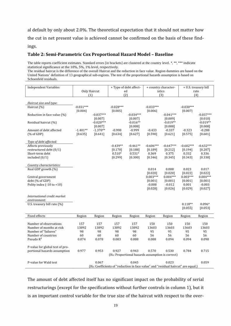
4.2. Baseline Estimation Results

Table 2 shows baseline estimation results for the full sample. The haircut measure used

here is computed according to the method by Sturzenegger and Zettelmeyer (2008).

Moreover, the estimations contain only those variables that have been shown to be suit-

able for inclusion into the Cox proportional hazard regressions in section 3. Specifically,

the variables included have been tested for significantly different and approximately

parallel Kaplan-Meier functions. The dummy variables indicating donor-funding, buy-

back deals, Brady deals and new money being included are disregarded in the estima-

tions due to potential endogeniety issues. All variables are described in more detail in

Table A1 in the Appendix. Table A2 provides some descriptive statistics.

Each regression is estimated twice: first, with the overall haircut as a regressor and, sec-

ond, with separate regressors for the cut in face value and the residual reduction in net

present value due to maturity extensions and/or interest rate cuts. Control variables are

included subsequently in table 2. Column 1 comprises only the haircuts, column 2 in-

cludes debt characteristics, countries’ economic and political fundamentals are included

in column 3, and the U.S. treasury bill rate as a proxy for international capital market

conditions is added in column 4. The estimation results are tested for robustness in sec-

tion 2.3.

The regression output confirms the descriptive findings as well as the IMF’s (2013)

claim that higher haircuts lead to a lower compound probability of follow-up restructur-

ings. A higher haircut in net present value of 1 percentage point is on average associated

with a (exp(−0.03) − 1) ∗ 100 = −3 % lower compound probability of observing a fol-

low-up restructuring. The IMF’s (2013) call for higher haircuts thus seems to be justi-

fied, if – as explained in the introductory section 1 – one assumes that a single haircut is

less expensive than serial restructurings (with the same aggregate haircut).

When discriminating between the effects of a haircut in face value and the residual hair-

cut due to maturity prolongation or/and interest rate reductions the coefficients are

both significantly negative but, surprisingly, we can reject the null hypothesis that they

are equal on the 5-10% significance levels, depending on the specification. This implies

that a reduction in face value has a stronger negative impact on the probability of serial

restructurings than a reduction of net present value due to maturity extension and/or

an interest rate reduction. While a one percentage point increase in the face value hair-

cut reduces the probability of a follow-up restructuring by 3.6%, an equally sized haircut

due to maturity extension and/or interest rate reduction reduces the probability of seri-

19

al default by only about 2.0%. The theoretical expectation that it should not matter how

the cut in net present value is achieved cannot be confirmed on the basis of these find-

ings.

Table 2: Semi-Parametric Cox Proportional Hazard Model – Baseline

The table reports coefficient estimates. Standard errors [in brackets] are clustered at the country level. *, **, *** indicate statistical significance at the 10%, 5%, 1% level, respectively. The residual haircut is the difference of the overall Haircut and the reduction in face value. Region dummies are based on the United Nations’ definition of 13 geographical sub-regions. The test of the proportional hazards assumption is based on Schoenfeld residuals. Independent Variables

Only Haircut (1)

+ Type of debt affect-ed (2)

+ country character-istics (3)

+ U.S. treasury bill rate (4)

Haircut size and type: Haircut (%) -0.031*** -0.028*** -0.033*** -0.030*** [0.004] [0.005] [0.006] [0.007] Reduction in face value (%) -0.037*** -0.034*** -0.041*** -0.037*** [0.007] [0.007] [0.009] [0.010] Residual haircut (%) -0.020*** -0.016** -0.019** -0.019** [0.007] [0.008] [0.008] [0.008] Amount of debt affected -1.401** -1.370** -0.998 -0.999 -0.433 -0.337 -0.323 -0.288 (% of GDP) [0.635] [0.641] [0.634] [0.627] [0.590] [0.621] [0.575] [0.601] Type of debt affected: Affects previously -0.439** -0.461** -0.606*** -0.647*** -0.602*** -0.632*** restructured debt (0/1) [0.170] [0.188] [0.189] [0.212] [0.194] [0.207] Short-term debt 0.510* 0.531* 0.369 0.375 0.332 0.336 included (0/1) [0.299] [0.300] [0.346] [0.345] [0.343] [0.338] Country characteristics: Real GDP growth (%) 0.014 0.008 0.023 0.017 [0.020] [0.020] [0.022] [0.022] Central government 0.003*** 0.004*** 0.003*** 0.004*** debt (% of GDP) [0.001] [0.001] [0.001] [0.001] Polity index (-10 to +10) -0.008 -0.012 0.001 -0.003 [0.028] [0.026] [0.029] [0.027] International credit market environment: U.S. treasury bill rate (%) 0.118** 0.096* [0.055] [0.053] Fixed effects Region Region Region Region Region Region Region Region Number of observations 157 157 157 157 150 150 150 150 Number of months at risk 13892 13892 13892 13892 13603 13603 13603 13603 Number of “failures” 98 98 98 98 95 95 95 95 Number of countries 60 60 60 60 56 56 56 56 Pseudo R² 0.074 0.078 0.083 0.088 0.088 0.094 0.094 0.098 P-value for global test of pro-portional hazards assumption 0.977 0.953 0.927 0.943 0.570 0.530 0.784 0.715 (H0: Proportional hazards assumption is correct) P-value for Wald test 0.067 0.045 0.023 0.059 (H0: Coefficients of “reduction in face value” and “residual haircut” are equal.)

The amount of debt affected itself has no significant impact on the probability of serial

restructurings (except for the specifications without further controls in column 1), but it

is an important control variable for the true size of the haircut with respect to the over-

20

all debt burden. Estimations where this variable is omitted nevertheless generate very

similar results (not shown here).

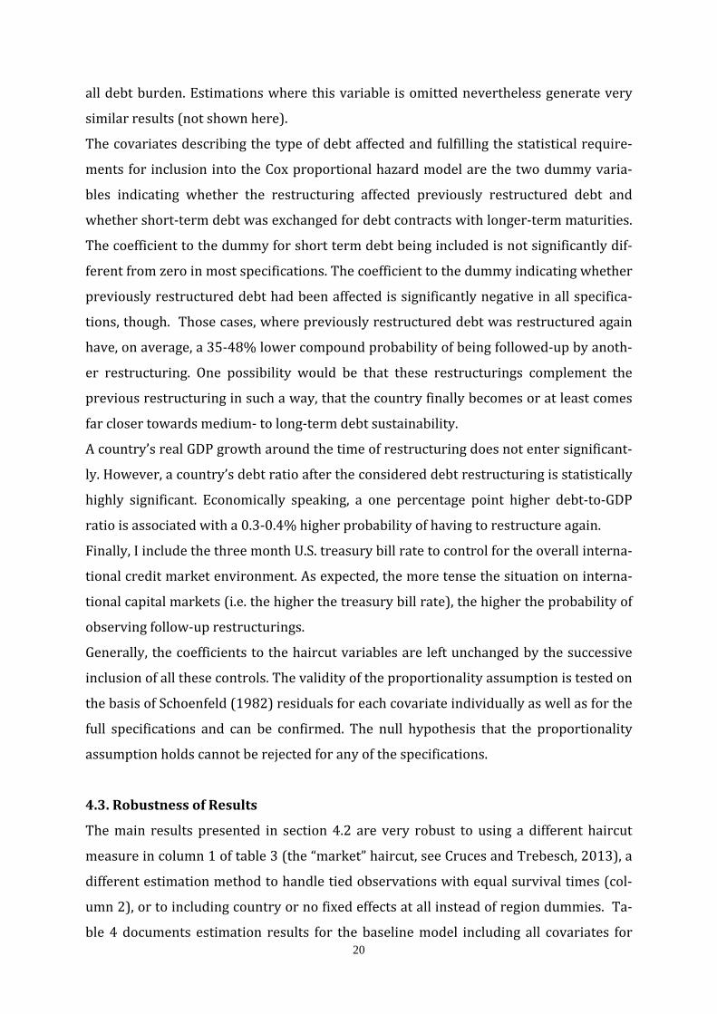
The covariates describing the type of debt affected and fulfilling the statistical require-

ments for inclusion into the Cox proportional hazard model are the two dummy varia-

bles indicating whether the restructuring affected previously restructured debt and

whether short-term debt was exchanged for debt contracts with longer-term maturities.

The coefficient to the dummy for short term debt being included is not significantly dif-

ferent from zero in most specifications. The coefficient to the dummy indicating whether

previously restructured debt had been affected is significantly negative in all specifica-

tions, though. Those cases, where previously restructured debt was restructured again

have, on average, a 35-48% lower compound probability of being followed-up by anoth-

er restructuring. One possibility would be that these restructurings complement the

previous restructuring in such a way, that the country finally becomes or at least comes

far closer towards medium- to long-term debt sustainability.

A country’s real GDP growth around the time of restructuring does not enter significant-

ly. However, a country’s debt ratio after the considered debt restructuring is statistically

highly significant. Economically speaking, a one percentage point higher debt-to-GDP

ratio is associated with a 0.3-0.4% higher probability of having to restructure again.

Finally, I include the three month U.S. treasury bill rate to control for the overall interna-

tional credit market environment. As expected, the more tense the situation on interna-

tional capital markets (i.e. the higher the treasury bill rate), the higher the probability of

observing follow-up restructurings.

Generally, the coefficients to the haircut variables are left unchanged by the successive

inclusion of all these controls. The validity of the proportionality assumption is tested on

the basis of Schoenfeld (1982) residuals for each covariate individually as well as for the

full specifications and can be confirmed. The null hypothesis that the proportionality

assumption holds cannot be rejected for any of the specifications.

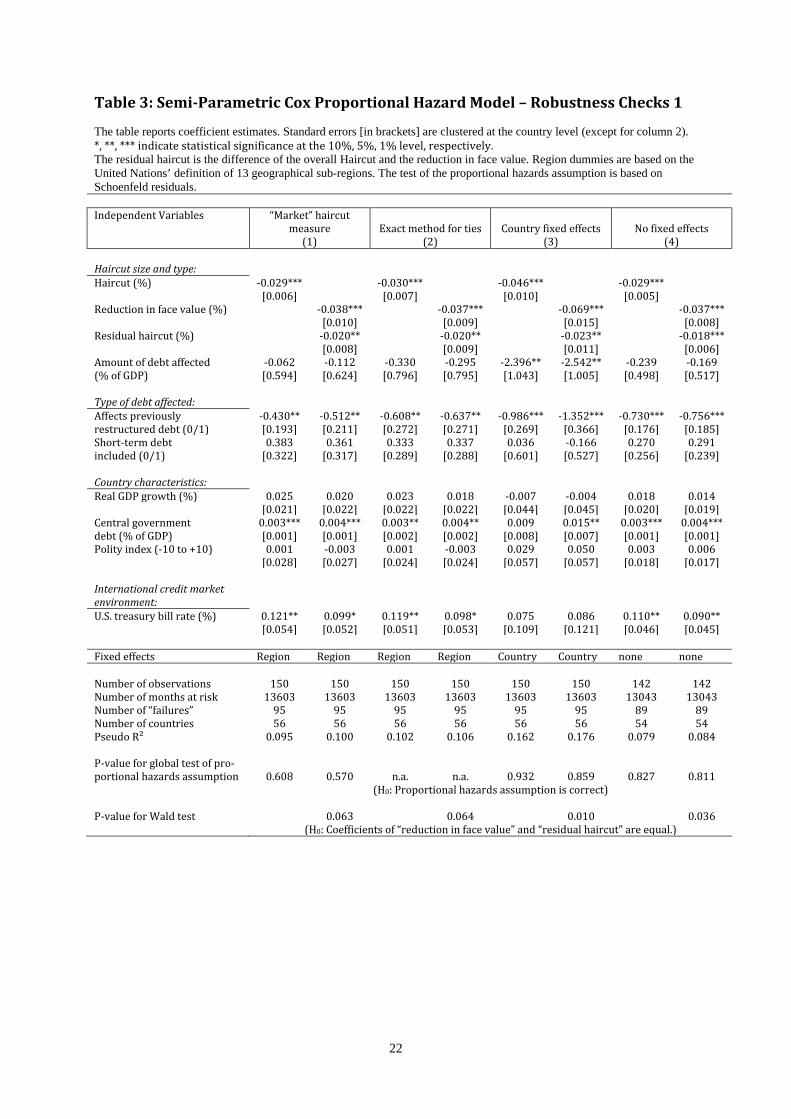
4.3. Robustness of Results

The main results presented in section 4.2 are very robust to using a different haircut

measure in column 1 of table 3 (the “market” haircut, see Cruces and Trebesch, 2013), a

different estimation method to handle tied observations with equal survival times (col-

umn 2), or to including country or no fixed effects at all instead of region dummies. Ta-

ble 4 documents estimation results for the baseline model including all covariates for

21

important subsamples, to check whether not controlling for other restructuring features

affects the results in any significant way because any variable omissions may lead to bi-

ased coefficients. Table 3 confirms all findings presented in section 4.2. Most important-

ly, higher haircuts lead to a lower probability of serial restructurings and the impact of

cuts in face value is significantly stronger than that of maturity extensions and/or inter-

est rate reductions. These effects are even more pronounced in the specification includ-

ing country dummies instead of region dummies (column 3). However, some of the oth-

er results from section 4.2 are lost in this specification. Note that, due to the large num-

ber of countries and the relatively small number of observations, the results from this

specification should be interpreted with caution.

The estimation results for different subsamples in table 4 further substantiate the main

results. The overall haircut as well as the cut in face value and the residual haircut all

enter negatively and (mostly) statistically significantly. The coefficients’ sizes are ex-

tremely similar to all previous estimations, too. Tests for the equality of the effects of a

cut in face value and the residual haircut largely confirm the above finding: The coeffi-

cient to a cut in face value is significantly larger in absolute value than the coefficient to

the residual haircut in the first two columns. Even though this significance is lost in col-

umns 3 and 4, the magnitudes of the coefficients remain very stable.

When running all the regressions using the full sample with a dummy variable control-

ling for a Brady deal, a donor-funded deal, a buy-back deal and/or a debt exchange in-

cluding the provision of new money (not shown here), results are still robust. The coeffi-

cient to this dummy variable is generally significantly negative.

Finally, tests for the validity of the proportional hazard assumption imply that specifica-

tions in tables 3 and 4 fulfill this critical assumption.

22

Table 3: Semi-Parametric Cox Proportional Hazard Model – Robustness Checks 1

The table reports coefficient estimates. Standard errors [in brackets] are clustered at the country level (except for column 2). *, **, *** indicate statistical significance at the 10%, 5%, 1% level, respectively. The residual haircut is the difference of the overall Haircut and the reduction in face value. Region dummies are based on the United Nations’ definition of 13 geographical sub-regions. The test of the proportional hazards assumption is based on Schoenfeld residuals. Independent Variables “Market” haircut

measure (1)

Exact method for ties (2)

Country fixed effects (3)

No fixed effects (4)

Haircut size and type: Haircut (%) -0.029*** -0.030*** -0.046*** -0.029*** [0.006] [0.007] [0.010] [0.005] Reduction in face value (%) -0.038*** -0.037*** -0.069*** -0.037*** [0.010] [0.009] [0.015] [0.008] Residual haircut (%) -0.020** -0.020** -0.023** -0.018*** [0.008] [0.009] [0.011] [0.006] Amount of debt affected -0.062 -0.112 -0.330 -0.295 -2.396** -2.542** -0.239 -0.169 (% of GDP) [0.594] [0.624] [0.796] [0.795] [1.043] [1.005] [0.498] [0.517] Type of debt affected: Affects previously -0.430** -0.512** -0.608** -0.637** -0.986*** -1.352*** -0.730*** -0.756*** restructured debt (0/1) [0.193] [0.211] [0.272] [0.271] [0.269] [0.366] [0.176] [0.185] Short-term debt 0.383 0.361 0.333 0.337 0.036 -0.166 0.270 0.291 included (0/1) [0.322] [0.317] [0.289] [0.288] [0.601] [0.527] [0.256] [0.239] Country characteristics: Real GDP growth (%) 0.025 0.020 0.023 0.018 -0.007 -0.004 0.018 0.014 [0.021] [0.022] [0.022] [0.022] [0.044] [0.045] [0.020] [0.019] Central government 0.003*** 0.004*** 0.003** 0.004** 0.009 0.015** 0.003*** 0.004*** debt (% of GDP) [0.001] [0.001] [0.002] [0.002] [0.008] [0.007] [0.001] [0.001] Polity index (-10 to +10) 0.001 -0.003 0.001 -0.003 0.029 0.050 0.003 0.006 [0.028] [0.027] [0.024] [0.024] [0.057] [0.057] [0.018] [0.017] International credit market environment: U.S. treasury bill rate (%) 0.121** 0.099* 0.119** 0.098* 0.075 0.086 0.110** 0.090** [0.054] [0.052] [0.051] [0.053] [0.109] [0.121] [0.046] [0.045] Fixed effects Region Region Region Region Country Country none none Number of observations 150 150 150 150 150 150 142 142 Number of months at risk 13603 13603 13603 13603 13603 13603 13043 13043 Number of “failures” 95 95 95 95 95 95 89 89 Number of countries 56 56 56 56 56 56 54 54 Pseudo R² 0.095 0.100 0.102 0.106 0.162 0.176 0.079 0.084 P-value for global test of pro-portional hazards assumption 0.608 0.570 n.a. n.a. 0.932 0.859 0.827 0.811 (H0: Proportional hazards assumption is correct) P-value for Wald test 0.063 0.064 0.010 0.036 (H0: Coefficients of “reduction in face value” and “residual haircut” are equal.)

23

Table 4: Semi-Parametric Cox Proportional Hazard Model – Robustness Checks 2

The table reports coefficient estimates. Standard errors [in brackets] are clustered at the country level. *, **, *** indicate statistical significance at the 10%, 5%, 1% level, respectively. The residual haircut is the difference of the overall Haircut and the reduction in face value. Region dummies are based on the United Nations’ definition of 13 geographical sub-regions. The test of the proportional hazards assumption is based on Schoenfeld residuals. Independent Variables

All 18 bond exchang-es excluded

(1)

All 17 Brady deals excluded

(2)

All 28 donor funded and/or buy-back deals excluded15

(3)

All 25 restructurings with provision of new

money excluded (4)

Haircut size and type: Haircut (%) -0.031*** -0.028*** -0.025*** -0.028*** [0.009] [0.006] [0.008] [0.006] Reduction in face value (%) -0.039*** -0.036*** -0.039** -0.035*** [0.013] [0.009] [0.017] [0.009] Residual haircut (%) -0.022** -0.017** -0.020** -0.020** [0.010] [0.008] [0.008] [0.008] Amount of debt affected -0.100 -0.107 0.080 0.141 -0.635 -0.424 -0.153 -0.041 (% of GDP) [0.626] [0.664] [0.843] [0.875] [0.653] [0.611] [0.887] [0.855] Type of debt affected: Affects previously -0.639*** -0.671*** -0.532** -0.609** -0.723*** -0.659*** -0.755*** -0.768*** restructured debt (0/1) [0.223] [0.231] [0.241] [0.260] [0.213] [0.231] [0.214] [0.219] Short-term debt 0.288 0.285 0.336 0.308 0.267 0.268 0.715* 0.718** included (0/1) [0.399] [0.390] [0.339] [0.351] [0.342] [0.332] [0.377] [0.363] Country characteristics: Real GDP growth (%) 0.025 0.020 0.019 0.013 0.020 0.017 0.019 0.013 [0.021] [0.022] [0.021] [0.022] [0.024] [0.023] [0.026] [0.026] Central government 0.004*** 0.005*** 0.003*** 0.004*** 0.004 0.004 0.003*** 0.004*** debt (% of GDP) [0.001] [0.002] [0.001] [0.001] [0.003] [0.003] [0.001] [0.001] Polity index (-10 to +10) 0.003 -0.001 -0.001 -0.005 0.003 -0.003 0.003 0.004 [0.031] [0.030] [0.032] [0.029] [0.028] [0.029] [0.030] [0.029] International credit market environment: U.S. treasury bill rate (%) 0.152** 0.131** 0.118** 0.095* 0.088 0.077 0.162*** 0.146** [0.065] [0.063] [0.055] [0.053] [0.054] [0.053] [0.060] [0.061] Fixed effects Region Region Region Region Region Region Region Region Number of observations 136 136 133 133 126 126 127 127 Number of months at risk 12866 12866 10498 10498 10337 10337 11835 11835 Number of “failures” 88 88 90 90 92 92 76 76 Number of countries 56 56 52 52 43 43 55 55 Pseudo R² 0.109 0.113 0.095 0.100 0.067 0.069 0.117 0.120 P-value for global test of pro-portional hazards assumption 0.475 0.283 0.985 0.997 0.401 0.025 0.868 0.907 (H0: Proportional hazards assumption is correct) P-value for Wald test 0.092 0.055 0.297 0.129 (H0: Coefficients of “reduction in face value” and “residual haircut” are equal.)

15 Many buy back deals are also donor funded, which is why these two categories largely overlap. Results are almost identical, if only one of the categories is excluded.

24

5. Conclusion

This paper complements existing empirical literature on sovereign debt restructurings

by analyzing whether the often stated claims that higher restructurings reduce the

probability of (near-term) follow-up restructurings are valid. I further distinguish be-

tween reductions in net present value of the debt in the form of cuts in face value as op-

posed to reductions in net present value due to maturity extensions or/and reductions

in interest rates. Finally, I investigate whether other restructuring features are correlat-

ed with the probability of serial restructurings.

The most important finding is that higher total debt remissions are significantly nega-

tively related to the probability of serial restructurings – most likely because higher debt

remissions move a country closer to a sustainable debt level than low alleviation. This

finding is rather straight forward and some studies already anticipated it (IMF, 2013;

Das et al., 2012; Moody’s, 2102). An immediate implication for future restructurings

would be that debtors and creditors should, whenever possible, dare to accept higher

debt remissions in order to prevent the debtor country from having to restructure over

and over again.

The estimation results also suggest that haircuts in face value reduce the probability of

serial restructurings by about twice as much as haircuts due to maturity extensions

or/and reductions in interest rates. This result refutes the theoretical logic that it is the

overall reduction in net present value which may impact a country’s debt sustainability,

no matter how this reduction comes about – a puzzle remaining to be explained in

greater detail by further research on this topic.

Unfortunately, the effects of donor funded restructurings, buy-back deals, brady deals

and restructurings including the provision of new money cannot be conclusively re-

solved because the expectations with respect to a country’s future debt sustainability

may e.g. drive decisions to provide funding along with granting debt relief. Nevertheless,

descriptive statistics show that these restructuring features are highly and significantly

correlated with a lower probability of serial restructurings.

25

References

Abbas , S. Ali, Nazim Belhocine, Asmaa ElGanainy, and Mark Horton. 2010. “A His-

torical Public Debt Database.” International Monetary Fund (IMF) Working Paper

10/245.

Aguiar, Mark, and Gita Gopinath. 2006. “Defaultable debt, interest rates and

the current account.” Journal of International Economics 69 (1): 64-83.

Arellano, Cristina. 2008. "Default Risk and Income Fluctuations in Emerging Econo-

mies." American Economic Review, 98(3): 690-712.

Arteta, Carlos, and Galina Hale. 2008. “Sovereign Debt Crises and Credit to the Private

Sector.” Journal of International Economics, 74 (1): 53-69

Asonuma, Tamon. 2010. “Serial Default and Debt Renegotiation.” Unpublished Paper,

Banco de Espana.

Borensztein, Eduardo, and Ugo Panizza. 2009. “The Costs of Sovereign Default.” IMF

Staff Papers 56 (4): 683-741

Cox, David R. (1972). “Regression Models and Life tables.” Journal of the Royal Statisti-

cal Society 34: 187-220.

Cruces, Juan J., and Christoph Trebesch. 2013. "Sovereign Defaults: The Price of Hair-

cuts." American Economic Journal: Macroeconomics 5 (3): 85-117.

Das, Udaibir S., Michael G. Papaioannou, and Christoph Trebesch. 2010. “Sovereign

Default Risk and Private Sector Access to Capital in Emerging Markets.” International

Monetary Fund (IMF) Working Paper 10/10.

Das, Udaibir S., Michael G. Papaioannou, and Christoph Trebesch. 2012. “Sovereign

Debt Restructurings 1950-2012: Literature Survey, Data, and Stylized Facts.” Interna-

tional Monetary Fund (IMF) Working Paper 12/203.

De Paoli, Bianca, Glenn Hoggarth, and Victoria Saporta. 2009. “Output costs of sov-

ereign crises: some empirical estimates.” Bank of England Working Paper 362.

Eaton, Jonathan, and Mark Gersovitz. 1981. "Debt with Potential Repudiation: Theo-

retical and Empirical Analysis." Review of Economic Studies 48 (2): 289-309.

Fuentes, Miguel, and Diego Saravia. 2010. “Sovereign defaulters: Do international

capital markets punish them?” Journal of Development Economics, 91 (2): 336-347.

Gelos, Gaston R., Guido Sandleris, and Ratna Sahay. 2011. “Sovereign borrowing by

developing countries: What determines market access?” Journal of International Eco-

nomics 83 (2): 243-254.

26

Gennaioli, Nicola, Alberto Martin, and Stefano Rossi. Forthcoming “Sovereign De-

fault, Domestic Banks, and Financial Institutions.” Journal of Finance, forthcoming.

Gianviti, François, Anne O. Krueger, Jean Pisani-Ferry, André Sapir, and Jürgen von

Hagen. 2010. "A European mechanism for sovereign debt crisis resolution: a proposal."

Bruegel Blueprint Series, Volume X.

IMF. 2013. Sovereign Debt Restructuring – Recent Developments and Implications for the

Fund’s Legal and Policy Framework. International Monetary Fund (IMF). Washington, DC,

April 26.

Krueger, Anne O. 2002. A New Approach To Sovereign Debt Restructuring. International

Monetary Fund (IMF). Washington, DC, April.

Levy-Yeyati, Eduardo, Maria S. Martinez Peria, and Sergio L. Schmukler. 2010. “De-

positor Behavior under Macroeconomic Risk: Evidence from Bank Runs in Emerging

Economies.” Journal of Money, Credit and Banking 42 (4): 585-614.

Levy-Yeyati, Eduardo, and Ugo Panizza. 2011. “The elusive costs of sovereign de-

faults.” Journal of Development Economics 94 (1): 95-105.

Marshall, Monty G., Keith Jaggers, Ted R. Gurr. 2011. “POLITY™ IV PROJECT – Politi-

cal Regime Characteristics and Transitions, 1800-2010.” Dataset Users’ Manual, Center

for Systemic Peace.

Martinez, Jose V., and Guido Sandleris. 2011. “Is it punishment? Sovereign defaults

and the decline in trade” Journal of International Money and Finance 30 (6): 909-930.

Mendoza, Enrique G., and Vivian Z. Yue. 2008. “A Solution to the Default Risk-

Business Cycle Disconnect” Board of Governors of the Federal Reserve System: Interna-

tional Finance Discussion Papers 924.

Moody’s. 2012. “Investor Losses in Modern-Era Sovereign Bond Restructurings.”

Soverign Defaults Series, Special Comment, August 7.

Panizza, Ugo, Federico Sturzenegger, and Jeromin Zettelmeyer. 2009. “The Eco-

nomics and Law of Sovereign Debt and Default.” Journal of Economic Literature 47 (3):

651-698.

Richmond, Christine, and Daniel A. Diaz. 2009. “Duration of Capital Market Exclusion:

An Empirical Investigation.” Unpublished Paper, University of Illinois at Urbana-

Champaign.

Rose, Andrew K. 2005. “One reason countries pay their debts: renegotiation and inter-

national trade.” Journal of Development Economics 77 (1): 189-206.

27

Schoenfeld D. 1982. “Residuals for the proportional hazards regression model.” Bio-

metrika 69(1): 239-241.

Sturzenegger, Frederico, and Jeromin Zettelmeyer. 2006. Debt Defaults and Lessons

from a Decade of Crises. Cambridge, MA: MIT Press.

Sturzenegger, Frederico, and Jeromin Zettelmeyer. 2008. “Haircuts: Estimating In-

vestor Losses in Sovereign Debt Restructurings, 1998-2005.” Journal of International

Money and Finance 27 (5): 780-805.

Tomz, Michael, and Mark L. J. Wright. 2007. “Do Countries Default in ‘Bad Times’?”

Journal of the European Economic Association 5 (2-3): 352-360.

Tomz, Michael, and Mark L. J. Wright. 2013. “Empirical Research on Sovereign Debt

and Default.” Annual Review of Economics 5(1): 247-272.

World Bank. 2007. Debt Reduction Facility for IDA-Only Countries: Progress Update and

Proposed Extension. World Bank Board Report 39310. Washington, DC, April.

Yue, Vivian Z. 2010. “Sovereign default and debt renegotiation.” Journal of International

Economics 80 (2): 176-187.

28

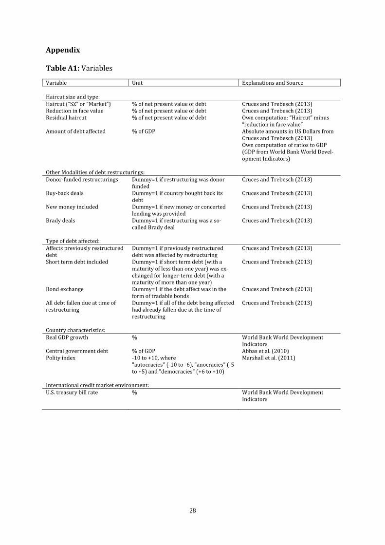
Appendix Table A1: Variables

Variable Unit Explanations and Source Haircut size and type: Haircut (“SZ” or “Market”) % of net present value of debt Cruces and Trebesch (2013) Reduction in face value % of net present value of debt Cruces and Trebesch (2013) Residual haircut % of net present value of debt Own computation: “Haircut” minus

“reduction in face value” Amount of debt affected % of GDP Absolute amounts in US Dollars from

Cruces and Trebesch (2013) Own computation of ratios to GDP (GDP from World Bank World Devel-opment Indicators)

Other Modalities of debt restructurings: Donor-funded restructurings Dummy=1 if restructuring was donor

funded Cruces and Trebesch (2013)

Buy-back deals Dummy=1 if country bought back its debt

Cruces and Trebesch (2013)

New money included Dummy=1 if new money or concerted lending was provided


Brady deals Dummy=1 if restructuring was a so-called Brady deal


Type of debt affected: Affects previously restructured debt

Dummy=1 if previously restructured debt was affected by restructuring


Short term debt included Dummy=1 if short term debt (with a maturity of less than one year) was ex-changed for longer-term debt (with a maturity of more than one year)


Bond exchange

Dummy=1 if the debt affect was in the form of tradable bonds


All debt fallen due at time of restructuring

Dummy=1 if all of the debt being affected had already fallen due at the time of restructuring


Country characteristics: Real GDP growth % World Bank World Development

Indicators Central government debt % of GDP Abbas et al. (2010) Polity index -10 to +10, where

"autocracies" (-10 to -6), "anocracies" (-5 to +5) and "democracies" (+6 to +10)

Marshall et al. (2011)

International credit market environment: U.S. treasury bill rate % World Bank World Development

Indicators

29

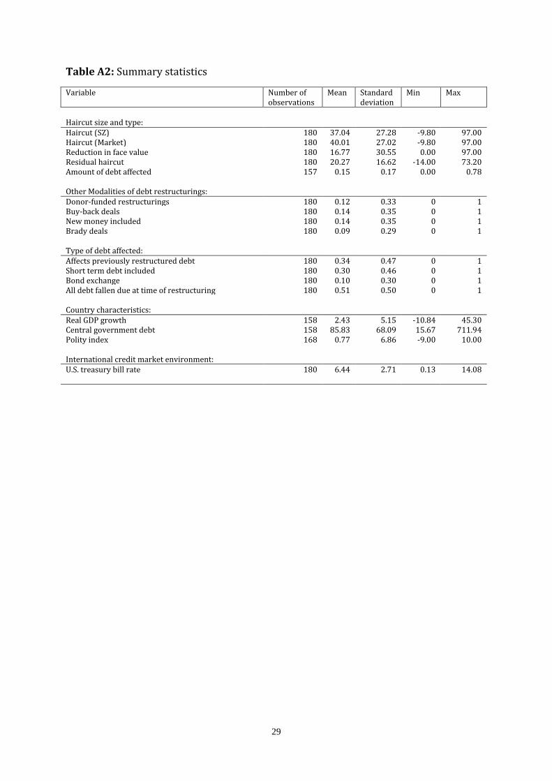
Table A2: Summary statistics

Variable Number of observations

Mean Standard deviation

Min Max

Haircut size and type: Haircut (SZ) 180 37.04 27.28 -9.80 97.00 Haircut (Market) 180 40.01 27.02 -9.80 97.00 Reduction in face value 180 16.77 30.55 0.00 97.00 Residual haircut 180 20.27 16.62 -14.00 73.20 Amount of debt affected 157 0.15 0.17 0.00 0.78 Other Modalities of debt restructurings: Donor-funded restructurings 180 0.12 0.33 0 1 Buy-back deals 180 0.14 0.35 0 1 New money included 180 0.14 0.35 0 1 Brady deals 180 0.09 0.29 0 1 Type of debt affected: Affects previously restructured debt 180 0.34 0.47 0 1 Short term debt included 180 0.30 0.46 0 1 Bond exchange 180 0.10 0.30 0 1 All debt fallen due at time of restructuring 180 0.51 0.50 0 1 Country characteristics: Real GDP growth 158 2.43 5.15 -10.84 45.30 Central government debt 158 85.83 68.09 15.67 711.94 Polity index 168 0.77 6.86 -9.00 10.00 International credit market environment: U.S. treasury bill rate 180 6.44 2.71 0.13 14.08

cesifo, a munich-based, globe-spanning economic research ......venice summer institute 2014 ... the...

Documents