Copyright © 2012 by ASME 1

INTRODUCTION

This work is a collaborative effort between the Biomechanics and

Living System Analysis Laboratory (BIOLISYS) in Cyprus and the

Biomechanics Laboratory of IACM/FORTH in Greece. Both labs

combine interdisciplinary skills from engineering, medicine and

biology to provide solutions to clinical problems associated with

cardiovascular and other diseases. For this study, numerical flow

simulations were performed using: a) open source software VMTK

and commercial software ICEM CFD as pre-processors, b) the finite

volume based solver Fluent and c) Tecplot 360 (Amtec Inc.) for post-

processing.

METHODS

Solver type and details

We used the finite volume solver Fluent v.12.1.4 (Ansys Inc.) for the

numerical approximation of the Navier-Stokes equations. For the

steady state cases the Coupled scheme was selected for pressure

velocity coupling using the pressure-based coupled solver. For the

transient solutions the PISO scheme was selected for the pressure

velocity coupling using the pressure-based segregated solver. We

apply the second order upwind scheme to discretise the convection

terms in the momentum equations and a second order pressure

interpolation scheme. A first order iterative time advancement scheme

is applied for the transient solutions. Gradients are computed using the

Green-Gauss node based method.

Mesh and boundary conditions

We use tools from VMTK to apply cylindrical flow extensions at the

inlet (Dinlet ~ 0.56 cm) and outlet of the domain so that we prescribe a

fully developed flow boundary condition at the inlet and a traction free

boundary condition at the outlet. The length of the outflow extension

was calculated based on the approximate relation for the entrance

length for steady laminar rigid pipe flow: Le/D~0.06Re where Le is the

entrance length, D is the tube diameter and Re the Reynolds number

[1]. In our case the maximum Re is 649 corresponding to a peak

systolic flow rate of 11.42 ml/s. Based on the outlet diameter (0.44

cm) the outflow length using the above relation should be at least 17

cm. An extension of 25 cm was applied.

We used ICEM CFD v12.1 (Ansys Inc.) to discretise the

computational domain and generate an unstructured mesh. The

computational domain (excluding flow extensions) is discretised with

~2.1 106 hybrid, linear elements with an average cell center spacing of

0.25 mm. Near-wall layers of prism elements were used throughout

the domain for boundary layer refinement with a 10-2 Dinlet distance of

the center of the first element from the wall. Triangles were used to

discretise the surface of the aneurysm and quads for the extensions.

Pyramid and tetrahedral elements were used to fill the core of the

computational domain in the aneurysm. The o-grid method was used

to generate layers of hexahedral elements in the flow extensions. A

parabolic velocity profile was applied at the inlet for the steady flow

cases with a mean velocity corresponding to the required flow rate.

For the transient flow cases the velocity profiles prescribed at the inlet

at each time step were obtain from the Womersley solution

(Womersley number~3.5) based on the flow waveform provided

(scaled appropriately to generate the desired mean flow rates) .

Steady-state flow computations were obtained on a HP Z800

workstation with 4 quadratic Intel Xeon processors in parallel. The

total CPU time was around 380 hrs corresponding to total wall clock

time of 95 hrs. Time varying solutions were obtained on an Intel Xeon

X5355 @ 2.66 GHz processor based Linux cluster requiring a total

CPU time of 75 hrs per flow cycle.

Grid size and time step independence study

We refined our mesh by reducing the mean cell center distance from

0.25 to 0.18 mm thus increasing the number of elements in the

aneurysm (excluding the extensions) from ~2.1 106 to ~4 106 and

Proceedings of the ASME 2012 Summer Bioengineering Conference SBC2012

June 20-23, Fajardo, Puerto Rico, USA

CFD CHALLENGE: SOLUTIONS USING THE COMMERCIAL FINITE VOLUME SOLVER,

FLUENT

Nicolas Aristokleous1, Mohammad Iman Khozeymeh

1, Yannis Papaharilaou

2, Georgios C.

Georgiou3, Andreas S. Anayiotos

1

1Department of Mechanical

Engineering and Materials Science

and Eng., Cyprus University of

Technology, Limassol, 3503, Cyprus

Proceedings of the ASME 2012 Summer Bioengineering Conference SBC2012

June 20-23, Fajardo, Puerto Rico

SBC2012-80691

1Department of Mechanical

Engineering and Materials Science

and Eng., Cyprus University of

Technology, Limassol, 3503, Cyprus

2Institute of Applied and Computational

Mathematics, Foundation for Research and

Technology – Hellas, Heraklion, Crete,

71110, Greece

3Department of Mathematics and

Statistics, University of Cyprus,

Nicosia, 1678, Cyprus

Copyright © 2012 by ASME 2

repeated our steady flow computations for the maximum flow case

(Q=11.42 ml/s). Our results indicated a maximum difference of less

than 1% in the computed centerline pressures between the coarse and

refined mesh. The initial mesh was thus considered sufficient.

A time step of 2.5 10-4 s was selected based on the expected peak

streamwise velocity and the mean element spacing in the aneurismal

sac. This corresponds to 3960 time-steps per flow cycle. To ensure

time step independence we repeated our transient computation for

Case 1 with a time step of 1.25 10-4 s or ½ the initial time step. The

maximum difference in the computed centerline pressures was less

than 1%.

Time periodicity and solution convergence

To exclude flow transients that appear during the early stages of the

numerical computation from our results we solve for 4 consecutive

flow cycles and present the results of the last cycle. We compared

peak systolic centerline pressures for the 3rd and 4th flow cycle and

found a maximum difference of less than 1% indicating that a time

periodic solution has been achieved in the fourth cycle. The total force

integrated over the aneurysm surface was also used as a measure to

verify time periodicity of the transient solution and convergence for

the steady flow case.

RESULTS

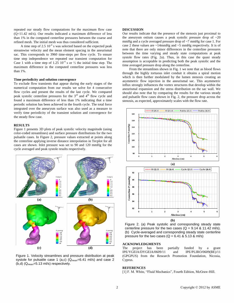
Figure 1 presents 3D plots of peak systolic velocity magnitude (using

color-coded streamlines) and surface pressure distributions for the two

pulsatile cases. In Figure 2, pressure values extracted at points along

the centerline applying inverse distance interpolation in Tecplot for all

cases are shown. Inlet pressure was set to 90 and 120 mmHg for the

cycle averaged and peak systole results respectively.

DISCUSSION

Our results indicate that the presence of the stenosis just proximal to

the aneurysm ostium causes a peak systolic pressure drop of ~20

mmHg and a cycle averaged pressure drop of ~7 mmHg for case 1. For

case 2 these values are ~14mmHg and ~5 mmHg respectively. It is of

note that there are only minor differences in the centerline pressures

between the time varying and steady state computations at peak

systole flow rates (Fig. 2a). Thus, in this case the quasi steady

assumption is acceptable in predicting both the peak systolic and the

time averaged pressure drop along the centerline.

From the streamlines shown in Fig. 1 we note that as blood flows

through the highly tortuous inlet conduit it obtains a spiral motion

which is then further modulated by the lumen stenosis creating an

asymmetric flow injection in the aneurismal sac. This asymmetric

influx strongly influences the vortex structures that develop within the

aneurismal expansion and the stress distribution on the sac wall. We

should also note that by comparing the results for the various steady

and pulsatile flow cases shown in Fig. 2, the pressure drop across the

stenosis, as expected, approximately scales with the flow rate.

ACKNOWLEDGMENTS

The project has been partially funded by a grant

IPE/YGEIA/DYGEIA/0609/11 and IPE/PLIRO/0609(BE)/11

(GPGPUS) from the Research Promotion Foundation, Nicosia,

Cyprus.

REFERENCES

[1] F. M. White, “Fluid Mechanics”, Fourth Edition, McGraw-Hill.

(a)

(b)

(c)

(d)

Figure 1. Velocity streamlines and pressure distribution at peak systole for pulsatile case 1 (a,c) (Qmean=6.41 ml/s) and case 2 (b,d) (Qmean=5.13 ml/s) respectively.

98

102

106

110

114

118

122

0 1 2 3 4 5 6

Abscissa (cm)

Cen

terl

ine

P (

mm

Hg)

SS Q9.14 SS Q11.42 PeakSys Q5.13 PeakSys Q6.41

(a)

82

84

86

88

90

92

0 1 2 3 4 5 6

Abscissa (cm)

Cen

terli

ne P

(m

mH

g)

SS Q5.13 SS Q6.41 CycAv Q5.13 CycAv Q6.41

(b)

Figure 2. (a) Peak systolic and corresponding steady state centerline pressure for the two cases (Q = 9.14 & 11.42 ml/s). (b) Cycle-averaged and corresponding steady state centerline pressure for the two cases (Q = 6.41 & 5.13 & ml/s)