CFD simulation of a safety relief valve for improvementof a one-dimensional valve model in RELAP5Master’s thesis in the Master’s program Innovative and Sustainable Chemical Engineering

ANNA BUDZISZEWSKILOUISE THOREN

Department of Applied PhysicsDivision of Nuclear EngineeringCHALMERS UNIVERSITY OF TECHNOLOGYGothenburg, Sweden 2012Master’s thesis CTH-NT-260

MASTER’S THESIS IN THE MASTER’S PROGRAM INNOVATIVE AND SUSTAINABLECHEMICAL ENGINEERING

CFD simulation of a safety relief valve for improvement of aone-dimensional valve model in RELAP5

ANNA BUDZISZEWSKILOUISE THOREN

Department of Applied PhysicsDivision of Nuclear Engineering

CHALMERS UNIVERSITY OF TECHNOLOGY

Gothenburg, Sweden 2012

CFD simulation of a safety relief valve for improvement of a one-dimensional valve model in RELAP5

ANNA BUDZISZEWSKILOUISE THOREN

c© ANNA BUDZISZEWSKI , LOUISE THOREN, 2012

Master’s thesis CTH-NT-260ISSN 1653-4662Department of Applied PhysicsDivision of Nuclear EngineeringChalmers University of TechnologySE-412 96 GothenburgSwedenTelephone: +46 (0)31-772 1000

Cover:The picture on the front page shows the safety relief valve including streamlines describing the fluidbehavior in the valve. The different colors of the streamlines represent the fluid velocity.

Chalmers ReproserviceGothenburg, Sweden 2012

CFD simulation of a safety relief valve for improvement of a one-dimensional valve model in RELAP5

Master’s thesis in the Master’s program Innovative and Sustainable Chemical EngineeringANNA BUDZISZEWSKILOUISE THORENDepartment of Applied PhysicsDivision of Nuclear EngineeringChalmers University of Technology

Abstract

In the Swedish nuclear power plants a structural verification of the pipe systems is a necessity toensure that the pipes are strong enough to withstand the forces which can result from a sudden event.One example of a component which generates forces in the systems while operating is the safety reliefvalve. Safety relief valves are used in order to prevent overpressure in a process system by releasing avolume of fluid from the process when a predetermined maximum pressure is reached.

In order to analyze the forces from water and steam in the pipe systems the software RELAP5, whichperforms calculations in one dimension, is commonly used within nuclear engineering. The valve modelwhich is currently used when simulating a safety relief valve in RELAP5 is the motor valve model. However,the usage of this model with present settings results in forces higher than in reality in the pipe systems.

The purpose of this project was to investigate how a safety relief valve can be modeled with CFD andto find interesting parameter relations to be implemented in RELAP5 in order to obtain more realisticresults of generated forces in the pipe systems. The aim was to modify the currently used motor valvemodel and to develop a servo valve model which is a more flexible model to use in RELAP5. The purposeof this project was also to investigate if a CFD simulation in 2D of the valve gives similar results as a 3Dsimulation.

The investigated valve in this project was a proportional valve. It starts to open at a set pressure of31 bar(g) and is completely opened at 10 % overpressure, i.e. 34.1 bar(g), where the maximum lift of8.5 mm is reached. The movement of the spindle is determined by the different forces acting on it. In thisproject the hydraulic forces, the spring force and the gravity force were considered.

The CFD simulations were performed in ANSYS FLUENT v.13. Dynamic layering was used in orderto change the mesh during the opening process of the valve. The 2D and 3D geometries were created andmeshed in ANSA v.13.2.1. Axisymmetry was used as a boundary condition in the 2D model, and in the3D model mirror symmetry was used. The used turbulence model was SST k − ω. A sensitivity analysiswas performed in order to investigate if and to which extent different mesh densities, turbulence modelsand time step sizes influence the results of the CFD simulations.

A verification of the 3D geometry and force calculations was performed, with the conclusion that theyseem to be consistent with reality. The transient 2D and 3D simulations were conducted with both aninstant and a gradual increase of inlet pressure. Differences could be observed between the 2D and 3Dsimulations but similarities were also evident. The simulations performed with a gradual increase of inletpressure were verified with experimental data. Interesting relations were found such as that the totalhydraulic force acting on the spindle is a function of different pressures in the valve and the mass flowthrough the valve.

In the currently used motor valve model in RELAP5 an opening time of 1 ms, an instant increase ofinlet pressure and the abrupt area change model are used. This model was modified by using an openingtime of 41 ms which was a result from the 3D CFD simulation. This modification resulted in lower forcesgenerated in the pipe right after the valve. The generated forces also reached more realistic magnitudesthan the forces generated from the currently used model.

A servo valve model was developed in RELAP5 by specifying all necessary relations, needed for thevalve to function, in control variables. One relation from the CFD simulations, describing the totalhydraulic force acting on the spindle, was implemented successfully. The usage of the abrupt area changemodel in combination with short pipes resulted in a stable system and realistic forces. The trends in theopening process were fairly consistent with reality when the inlet pressure was gradually increased.

Both the motor and the servo valve model were also modified by using the smooth area change modelincluding the implementation of a Cv table. This modification did not decrease the magnitude of theforces and instabilities were observed in the system.

The opening process of the valve, simulated both with CFD and in RELAP5, is faster than the openingprocess observed in experimental data. This concludes that the models are conservative, which is arequirement within the nuclear industry.

Keywords: Safety relief valve, Computational Fluid Dynamics, RELAP5, Nuclear engineering, Dynamiclayering, UDF

ii

Preface

This Master of Science thesis has been performed by Anna Budziszewski and Louise Thoren, studentsat the Master’s program Innovative and Sustainable Chemical Engineering at Chalmers University ofTechnology in Gothenburg, Sweden. The thesis has been performed at FS Dynamics in collaborationwith the Department of Applied Physics at Chalmers University of Technology during spring 2012. TheMaster’s thesis was supervised by Anna Nystrom and Mattias Wangblad at FS Dynamics, and theexaminer at Chalmers University of Technology was Christophe Demaziere.

Acknowledgements

First of all, we would like to express our gratitude to our supervisors Anna Nystrom and Mattias Wangbladat FS Dynamics for their commitment and help during the project. We would also like to thank ourexaminer Christophe Demaziere at Chalmers University of Technology for his encouragement and support.

We would like to thank Mikael Stallgard and Fredrik Carlsson at FS Dynamics and Bengt Anderssonat Chalmers University of Technology for their helpful discussions regarding difficulties we have run intoduring the CFD simulations. We would also like to thank Anders Bystrom at Ringhals NPP for providingus with the original drawing of the valve and experimental data enabling us to validate our CFD models.

We would also like to thank Ori Levin at FS Dynamics for the great discussions and all the supportregarding the RELAP5 simulations of the valve. Without his help we would never have finished the servovalve model on time. We would also like to give a great thank you to Fredrik Larsson at FS Dynamics ITsupport who have helped us with all computational problems we have run into (or caused). We wouldalso like to thank Ulf Engdar and Fredrik Erling for giving feedback on the report, and Linn Svard for thesupport during the writing of the report.

Lastly, we would like to show our appreciation to everyone at FS Dynamics for their warm welcomingand enjoyable discussions during lunchtime.

Gothenburg, June 8, 2012Anna Budziszewski and Louise Thoren

iii

iv

Nomenclature

Roman

A area [m2]ac layer collapse factor [−]as layer split factor [−]

Cv flow coefficient used in RELAP5 [m3/s√Pa

]

F force [N ]g gravity [m/s2]h cell height [m]k spring constant [N/m]k kinetic energy [J ]K energy loss coefficient [−]l turbulent length scale [m]L pipe length [m]m mass [kg]P pressure [Pa]t time [s]T temperature [K]U fluid velocity [m/s]u turbulent fluid velocity [m/s]v velocity of the spindle [m/s]x lift of the spindle [m]

Greek

α volume fraction of gas or liquid [−]ε energy dissipation rate [m2/s3]µ molecular viscosity [kg/(m · s)]µf friction coefficient [−]ν kinematic viscosity [m2/s]νT turbulent viscosity [m2/s]ρ density [kg/m3]τT Reynolds stresses [N/m2]τ viscous stresses [N/m2]ω specific dissipation [1/s]Γ volumetric mass exchange rate [kg/(m3 · s)]

Abbreviations

CFD Computational Fluid DynamicsSST Shear Stress TransportUDF User Defined Function6DOF Six Degree Of Freedom

v

vi

Contents

Abstract i

Preface iii

Acknowledgements iii

Nomenclature v

Contents vii

1 Introduction 1

1.1 Purpose . . . . . . . . . . . . . . . . . . . . . . . . . . . . . . . . . . . . . . . . . . . . . . . . 1

1.2 Constraints . . . . . . . . . . . . . . . . . . . . . . . . . . . . . . . . . . . . . . . . . . . . . . 1

1.3 Method . . . . . . . . . . . . . . . . . . . . . . . . . . . . . . . . . . . . . . . . . . . . . . . . 2

2 Safety relief valves 3

2.1 Design . . . . . . . . . . . . . . . . . . . . . . . . . . . . . . . . . . . . . . . . . . . . . . . . . 3

2.2 Lifting and reseating . . . . . . . . . . . . . . . . . . . . . . . . . . . . . . . . . . . . . . . . . 4

2.3 Movement of the spindle . . . . . . . . . . . . . . . . . . . . . . . . . . . . . . . . . . . . . . . 5

2.3.1 Forces acting on the spindle . . . . . . . . . . . . . . . . . . . . . . . . . . . . . . . . . . . . 5

2.3.2 Forces considered in this project . . . . . . . . . . . . . . . . . . . . . . . . . . . . . . . . . 7

3 Geometry and meshing 9

3.1 Geometry . . . . . . . . . . . . . . . . . . . . . . . . . . . . . . . . . . . . . . . . . . . . . . . 9

3.2 Meshing . . . . . . . . . . . . . . . . . . . . . . . . . . . . . . . . . . . . . . . . . . . . . . . . 11

3.2.1 y+ value . . . . . . . . . . . . . . . . . . . . . . . . . . . . . . . . . . . . . . . . . . . . . . 11

3.2.2 2D model . . . . . . . . . . . . . . . . . . . . . . . . . . . . . . . . . . . . . . . . . . . . . . 11

3.2.3 3D model . . . . . . . . . . . . . . . . . . . . . . . . . . . . . . . . . . . . . . . . . . . . . . 13

4 CFD simulations of a safety relief valve 14

4.1 Governing equations . . . . . . . . . . . . . . . . . . . . . . . . . . . . . . . . . . . . . . . . . 14

4.1.1 Continuity equation . . . . . . . . . . . . . . . . . . . . . . . . . . . . . . . . . . . . . . . . 14

4.1.2 Momentum equation . . . . . . . . . . . . . . . . . . . . . . . . . . . . . . . . . . . . . . . . 14

4.2 Modeling of turbulent flow . . . . . . . . . . . . . . . . . . . . . . . . . . . . . . . . . . . . . . 15

4.2.1 Realizable k − ε model . . . . . . . . . . . . . . . . . . . . . . . . . . . . . . . . . . . . . . . 16

4.2.2 Shear Stress Transport (SST) k − ω model . . . . . . . . . . . . . . . . . . . . . . . . . . . 17

4.3 Near wall flow . . . . . . . . . . . . . . . . . . . . . . . . . . . . . . . . . . . . . . . . . . . . . 17

4.4 Dynamic mesh . . . . . . . . . . . . . . . . . . . . . . . . . . . . . . . . . . . . . . . . . . . . 17

4.4.1 Dynamic layering . . . . . . . . . . . . . . . . . . . . . . . . . . . . . . . . . . . . . . . . . . 18

4.4.2 User Defined Function . . . . . . . . . . . . . . . . . . . . . . . . . . . . . . . . . . . . . . . 19

5 One-dimensional simulations of a safety relief valve 20

5.1 Governing equations . . . . . . . . . . . . . . . . . . . . . . . . . . . . . . . . . . . . . . . . . 20

5.1.1 Phasic continuity equations . . . . . . . . . . . . . . . . . . . . . . . . . . . . . . . . . . . . 20

5.1.2 Phasic momentum equations . . . . . . . . . . . . . . . . . . . . . . . . . . . . . . . . . . . 21

5.2 Modeling of valves in RELAP5 . . . . . . . . . . . . . . . . . . . . . . . . . . . . . . . . . . . 21

5.2.1 Motor and servo valve models . . . . . . . . . . . . . . . . . . . . . . . . . . . . . . . . . . . 22

5.3 Force calculations . . . . . . . . . . . . . . . . . . . . . . . . . . . . . . . . . . . . . . . . . . . 23

vii

6 Settings used in the CFD and RELAP5 simulations 246.1 Initial valve opening of 5 % . . . . . . . . . . . . . . . . . . . . . . . . . . . . . . . . . . . . . 246.2 Spring settings . . . . . . . . . . . . . . . . . . . . . . . . . . . . . . . . . . . . . . . . . . . . 246.3 Mass of spindle . . . . . . . . . . . . . . . . . . . . . . . . . . . . . . . . . . . . . . . . . . . . 246.4 Mesh . . . . . . . . . . . . . . . . . . . . . . . . . . . . . . . . . . . . . . . . . . . . . . . . . . 256.5 Numerical settings in ANSYS FLUENT . . . . . . . . . . . . . . . . . . . . . . . . . . . . . . 256.6 Numerical settings in RELAP5 . . . . . . . . . . . . . . . . . . . . . . . . . . . . . . . . . . . 26

7 Sensitivity analysis of the CFD simulations 287.1 Mesh density . . . . . . . . . . . . . . . . . . . . . . . . . . . . . . . . . . . . . . . . . . . . . 287.2 Turbulence models and time step sizes . . . . . . . . . . . . . . . . . . . . . . . . . . . . . . . 29

8 Results 328.1 Verification of 3D geometry and force calculations . . . . . . . . . . . . . . . . . . . . . . . . 328.2 CFD simulations of the safety relief valve . . . . . . . . . . . . . . . . . . . . . . . . . . . . . 338.2.1 3D model - Instant increase of inlet pressure . . . . . . . . . . . . . . . . . . . . . . . . . . 338.2.2 2D model - Instant increase of inlet pressure . . . . . . . . . . . . . . . . . . . . . . . . . . 428.2.3 Gradual increase of inlet pressure . . . . . . . . . . . . . . . . . . . . . . . . . . . . . . . . . 458.3 One-dimensional simulations of the safety relief valve . . . . . . . . . . . . . . . . . . . . . . . 538.3.1 Motor valve model . . . . . . . . . . . . . . . . . . . . . . . . . . . . . . . . . . . . . . . . . 538.3.2 Servo valve model . . . . . . . . . . . . . . . . . . . . . . . . . . . . . . . . . . . . . . . . . 55

9 Overall discussion 609.1 Conclusions . . . . . . . . . . . . . . . . . . . . . . . . . . . . . . . . . . . . . . . . . . . . . . 619.2 Future studies . . . . . . . . . . . . . . . . . . . . . . . . . . . . . . . . . . . . . . . . . . . . . 61

A Appendix - UDF 63A.1 UDF for CFD simulation in 3D . . . . . . . . . . . . . . . . . . . . . . . . . . . . . . . . . . . 63A.2 UDF for CFD simulation in 2D . . . . . . . . . . . . . . . . . . . . . . . . . . . . . . . . . . . 68

B Appendix - Motor valve model 73B.1 Currently used motor valve model . . . . . . . . . . . . . . . . . . . . . . . . . . . . . . . . . 73B.2 Motor valve model with abrupt area change and 41 ms opening time . . . . . . . . . . . . . . 77B.3 Motor valve model with smooth area change and 41 ms opening time . . . . . . . . . . . . . . 77

C Appendix - Servo valve model 78

viii

1 IntroductionAll pressurized systems require safety devices in order to protect people, processes and properties. As soonas mankind was able to boil water to create steam, the necessity of the safety device became evident. Earlyin the 19th century, boiler explosions on ships and locomotives frequently resulted from non-working safetydevices, which led to the development of the first safety relief valves. In order to prevent overpressure in asystem the safety relief valve is an important type of device. The safety relief valve operates by releasinga volume of fluid from within the system when a predetermined maximum pressure is reached, therebyreducing the excess pressure in a safe way [1].

Safety relief valves are today used in all types of process plants, and nuclear power plants constitutesuch an example. In the Swedish nuclear power plants a structural verification of the pipe systems isa necessity to ensure that the pipes are strong enough to withstand the forces which can result from asudden event. A typical pipe system in a nuclear power plant consists of several process componentswhich generate forces in the pipe system while operating. The safety relief valve is one example of such acomponent.

In order to analyze the forces from water and steam in the pipe systems in a nuclear power plant, thesoftware RELAP5 is commonly used. RELAP5 is used for modeling of process systems and is performingone-dimensional calculations. In RELAP5 a valve is modeled as a junction between two pipes. The modelwhich is currently used when simulating the effects of a safety relief valve in RELAP5 is the motor valvemodel, where flow coefficients and opening rates are specified. However, the usage of this model withpresent settings results in forces higher than in reality in the pipe systems, since the simulated valve opensfaster than what is physically possible. Unstable solutions are sometimes also a result from the usage ofthis model with present settings.

1.1 Purpose

To achieve more realistic results, when investigating the forces from water and steam in nuclear pipesystems, the currently used valve model needs to be improved. This can be accomplished by simulatingthe safety relief valve with CFD and integrating the results with the currently used model in RELAP5.The purpose of this project is therefore to investigate how a safety relief valve can be modeled in 3D inANSYS FLUENT and to find what parameters are important in order to obtain a realistic 1D model inRELAP5. The aim is to modify the existing motor valve model and to compare the new settings withthe currently used settings. In addition to the modification of the motor valve model another aim is todevelop a servo valve model which is a more flexible model to use when investigating effects of valves inRELAP5. The purpose of this project is also to investigate if a 2D simulation of the valve in ANSYSFLUENT will give similar results as the 3D simulation, which would make future simulations easier andwould require less computational time.

1.2 Constraints

This project has the following restrictions:

• The fluid flowing through the safety relief valve is chosen to be liquid water, which is assumed to beincompressible in the CFD simulations.

• In order to avoid phase changes in the system the water is assumed to be at ambient temperature of25◦C.

• It is assumed that there is water in the entire system (both at the inlet and outlet of the valve) asinitial condition of the simulations.

• Due to fluid structure interactions fluid and solid domains will affect each other. However, thedeformation of the solid parts will not be considered in this project.

• Only the opening process of the valve is considered.

• Damping of the valve is not considered during the simulations, due to lack of data.

1

1.3 Method

The safety relief valve was simulated in ANSYS FLUENT v.13 and the valve was simulated in both 2Dand 3D. The geometries were drawn and meshed in ANSA v.13.2.1. To check if the 3D geometry wascorrect, steady state simulations were performed at specific magnitudes of lift of the spindle and thecalculated total force acting on the spindle was compared with experimental data. Transient simulationswere performed in order to investigate the dynamic behavior of the safety relief valve and the dynamiclayering method was used. The transient simulations were performed with both an instant and a gradualincrease of the inlet pressure. A sensitivity analysis was also carried out in order to investigate theinfluence of different parameters on the simulations. By using data from the transient simulations inANSYS FLUENT, the motor valve model in RELAP5 was modified and a servo valve model was developed.The modified motor valve model was compared with the currently used motor valve model by observingthe forces generated in the pipe system created due to the opening of the valve. The developed servovalve model was compared with the 3D CFD model and experimental data.

2

2 Safety relief valves

Safety relief valves are used in order to prevent overpressure in a process system by releasing a volumeof fluid from the process when a predetermined maximum pressure is reached. The excess pressure isthereby reduced in a safe manner.

A wide range of different safety relief valves are available for many different applications and performancecriteria. A safety relief valve is generally characterized by rapid opening (pop action/full lift), or byopening proportionally to the increase of overpressure. The full lift safety relief valve is mainly used forcompressible fluids and the proportional valve for incompressible fluids [1].

2.1 Design

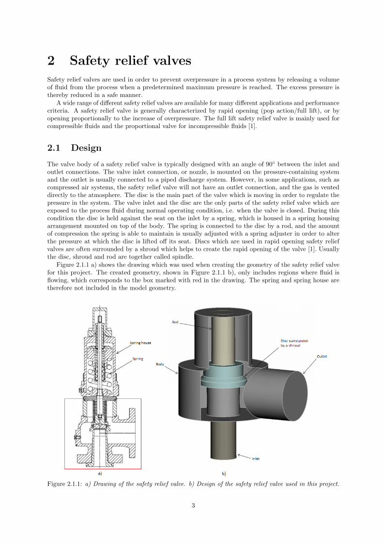
The valve body of a safety relief valve is typically designed with an angle of 90◦ between the inlet andoutlet connections. The valve inlet connection, or nozzle, is mounted on the pressure-containing systemand the outlet is usually connected to a piped discharge system. However, in some applications, such ascompressed air systems, the safety relief valve will not have an outlet connection, and the gas is venteddirectly to the atmosphere. The disc is the main part of the valve which is moving in order to regulate thepressure in the system. The valve inlet and the disc are the only parts of the safety relief valve which areexposed to the process fluid during normal operating condition, i.e. when the valve is closed. During thiscondition the disc is held against the seat on the inlet by a spring, which is housed in a spring housingarrangement mounted on top of the body. The spring is connected to the disc by a rod, and the amountof compression the spring is able to maintain is usually adjusted with a spring adjuster in order to alterthe pressure at which the disc is lifted off its seat. Discs which are used in rapid opening safety reliefvalves are often surrounded by a shroud which helps to create the rapid opening of the valve [1]. Usuallythe disc, shroud and rod are together called spindle.

Figure 2.1.1 a) shows the drawing which was used when creating the geometry of the safety relief valvefor this project. The created geometry, shown in Figure 2.1.1 b), only includes regions where fluid isflowing, which corresponds to the box marked with red in the drawing. The spring and spring house aretherefore not included in the model geometry.

Figure 2.1.1: a) Drawing of the safety relief valve. b) Design of the safety relief valve used in this project.

3

2.2 Lifting and reseating

The maximum pressure in the system for which the spindle remains in its original position attachedto the seat of the inlet is called the set pressure. When the inlet static pressure rises above the setpressure of the safety relief valve, the disc will begin to lift off its seat. As soon as the spindle startsto lift the spring compresses and the spring force increases. This means that the fluid pressure has toincrease beyond the set pressure in order to lift the spindle further. The additional pressure rise, above setpressure, is called the overpressure. The overpressure required to open the valve completely is different fordifferent valves and applications. When the fluid is compressible, the overpressure for a fully open valve isnormally between 3 % and 10 % of the set pressure. For incompressible fluids the overpressure is normallybetween 10 % and 25 % [1]. In this project the set pressure is 31 bar(gauge) and the overpressure is 10 %which means that the valve will start to open at a pressure higher than 31 bar(g) and be fully open at34.1 bar(g). As the spindle lifts the lower surface of the shroud changes the direction of the flow providinga dynamic force which further enhances the lift of the spindle.

Once acceptable operating conditions have been restored in the system, the valve should close again.But since a larger area of the spindle is exposed to the fluid when the valve is open, the valve will notclose until the pressure has dropped below the original set pressure. This phenomenon is called hysteresis.The difference between the set pressure and the reseating pressure is called the blowdown, and it is usuallyspecified as a percentage of the set pressure. For compressible fluids, the blowdown is usually less than10 %, and for incompressible fluids it can be up to 20 % of set pressure [1]. However, the closing of thevalve in this project is not considered.

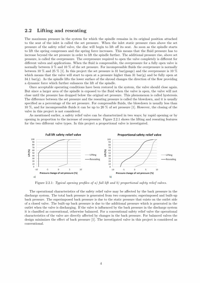
As mentioned earlier, a safety relief valve can be characterized in two ways; by rapid opening or byopening in proportion to the increase of overpressure. Figure 2.2.1 shows the lifting and reseating featuresfor the two different valve types. In this project a proportional valve is investigated.

Figure 2.2.1: Typical opening profiles of a) full lift and b) proportional safety relief valves.

The operational characteristics of the safety relief valve may be affected by the back pressure in thedischarge system. The total back pressure is generated from two components; superimposed and built-upback pressure. The superimposed back pressure is due to the static pressure that exists on the outlet sideof a closed valve. The built-up back pressure is due to the additional pressure which is generated in theoutlet when the valve is discharging. If the valve is influenced by the back pressure in the discharge systemit is classified as conventional, otherwise balanced. For a conventional safety relief valve the operationalcharacteristics of the valve are directly affected by changes in the back pressure. For balanced valves thedesign minimizes the effect of back pressure [1]. The investigated valve in this project is considered asconventional.

4

2.3 Movement of the spindle

The movement of the spindle can be described with Newton’s Second Law, see equation (2.3.1).

F = ma = mdv

dt(2.3.1)

By integrating equation (2.3.1) the expression for the velocity of the spindle becomes

vt = vt−∆t +F

m∆t (2.3.2)

It is here assumed that the force remains constant during ∆t.

2.3.1 Forces acting on the spindle

Since the spindle only can move in one direction the motion of the spindle is determined by the forcesacting on it in the direction of movement, i.e. vertically in this project. These forces are;

• Fhydraulic,1 – Fluid pressure forces acting on the lower surface of the disc and shroud

• Fhydraulic,2 – Fluid pressure forces acting on the upper surface of the shroud

• Fviscous – Forces acting on the surface of the spindle due to the movement of the fluid

• Fspring – Force due to the compression of the spring

• Fgravity – Force due to the weight of the spindle under gravity

• Ffriction – Friction force between solid moving parts

• Fdamping – Force due to friction elements which function is to slow down rapid motions of the spindle

• Fspringhouse – Pressure force acting on the top of the rod due to the pressure inside the spring house

The net force acting on the spindle is

F = Fhydraulic,1 +Fhydraulic,2 +Fviscous+Fspring +Fgravity +Ffriction+Fdamping +Fspringhouse (2.3.3)

Hydraulic forcesA major force causing the disc to lift off its seat is the fluid pressure force acting on the lower surface ofthe spindle, Fhydraulic,1, resulting in a lifting force. Fhydraulic,2 is mainly due to the back pressure in thevalve. A momentum balance on a body in a fluid shows that the magnitude of the hydraulic forces can beexpressed as follows

Fhydraulic = PA (2.3.4)

This shows that the magnitude of the hydraulic force is equal to the product of the pressure in the fluidand the area exposed to the fluid [1]. When the lift begins, a larger area of the lower surface of thespindle is exposed to the fluid pressure from the valve inlet and the opening force Fhydraulic,1 is thereforeincreasing as the valve opens. Figure 2.3.1 shows the difference in exposed area between a closed and anopen valve respectively.

5

Figure 2.3.1: A larger area of the spindle is exposed to the fluid in open position than in closed position,which results in a larger hydraulic force from beneath, Fhydraulic,1.

When the fluid enters the chamber in the valve body, the back pressure increases. Fhydraulic,2, whichis due to the back pressure in the valve will therefore increase with higher lift and hence reduce the totallift force on the spindle.

Viscous forcesThe viscous forces, also called shear forces, are acting on the surfaces of the spindle as a result of themovement of the fluid surrounding the spindle. The force is acting in the same direction as the fluid flowsaround the spindle. The shear force can be expressed as

Fviscous = τA (2.3.5)

The viscous stress, τ , is a tensor quantity which requires magnitude, direction, and orientation withrespect to a plane for identification. The stress is identified by two directions, indicated by the subscriptsi and j. One of the subscripts is indicating the direction perpendicular to the plane of action and theother is indicating the direction of the plane of action [2]. For Newtonian fluids such as water, the shearstress can be expressed as

τij = µ

(∂Ui∂xj

+∂Uj∂xi

)(2.3.6)

where µ is the molecular viscosity.

Spring forceDuring valve opening the spring force, Fspring, increases due to the compression of the spring. The springforce can be described with Hooke’s law, equation (2.3.7).

Fspring = −kx (2.3.7)

where k is the spring constant and x is the compression of the spring. At the equilibrium position of thespring the spring force is equal to 0 N. However, in a safety relief valve the spring will never be in itsequilibrium position. In this type of valve it is crucial that the valve remains closed until the set pressureis reached. Therefore, an initial tension force is applied on the spring which keeps the spring compressedeven at closed valve position and not only during discharge of fluid. For a safety relief valve the springforce expression can instead be written as

Fspring = −(F0 + kxlift) = −k(x0 + xlift) (2.3.8)

where F0=kx0 is the initial tension force and x0 is the initial compression of the spring.

Gravity forceAll objects with a mass are affected by the gravity, resulting in a force which magnitude can be expressedas

Fgravity = mg (2.3.9)

6

Friction forcesFriction is the force resisting the relative motion of solid surfaces sliding against each other [3]. Themagnitude of the force can be expressed as

Ffriction = µfFn (2.3.10)

where µf is the coefficient of friction and Fn is the normal force.

Damping forceIn valves where unstable features can be observed such as fluttering or chattering a damper device maybe used. The damper is attached to the rod inside the spring house and eliminates valve stem oscillations[4]. In the safety relief valve used in this project a smaller spring in combination with friction elementsform the damper device.

Pressure forceThe pressure inside the spring house is causing a pressure force acting on the top of the rod. This forceis acting in the opposite direction of the lifting of the spindle and is therefore reducing the total liftforce acting on the spindle. The magnitude of this pressure force can be expressed with equation (2.3.4)where A is the cross-sectional area of the rod and P is the pressure in the spring house. In this projectatmospheric pressure is prevailing inside the spring house.

2.3.2 Forces considered in this project

In this project only the hydraulic forces, the spring force and the gravity force are taken into account.The pressure force from the pressure inside the spring house is constant and is included in the initialtension, F0, of the spring. The contributions from the viscous and friction forces are assumed to be verysmall compared to the other forces and are therefore neglected in the model. The damping forces areneglected since no data was available, which made it impossible to include in the model. The net forceacting on the spindle in this project is therefore

F = Fhydraulic,1 + Fhydraulic,2 + Fspring + Fgravity (2.3.11)

Figure 2.3.2 shows a schematic picture of the valve where the forces considered in this project are included.

7

Figure 2.3.2: Considered forces acting on the spindle in this project.

8

3 Geometry and meshingIn this chapter the geometry of the safety relief valve model is described. Furthermore, the meshingprocedure is explained and the meshes of the 2D and 3D models are presented. The meshes are used inorder to perform simulations in ANSYS FLUENT.

3.1 Geometry

In this project the geometry of the safety relief valve has been created in ANSA v.13.2.1. ANSA is aCAE (Computer-Aided Engineering) preprocessing tool developed by BETA CAE Systems. The softwareis typically used for cleanup and refinement of CAD geometries and has the ability to generate meshesof high quality [5]. ANSA can also be used to create geometries from scratch, which is the case in thisproject since a CAD drawing was not available. By using the dimensions given in the original drawingfrom a valve manufacturer the 2D and 3D geometries of the valve were created. Some simplifications ofthe valve were made in order to make the meshing easier and more structured. Two examples of thesimplifications are sharper edges and the neglect of small structures. Figure 3.1.1 shows a) the availabledrawing and b) the simplified geometry created in ANSA including the dimensions used. Figure 3.1.2shows a close-up of the spindle and its dimensions. All dimensions are presented in Table 3.1.1.

Figure 3.1.1: a) Original drawing and b) geometry created in ANSA.

9

Figure 3.1.2: Close-up of the spindle.

Table 3.1.1: Dimensions of the geometry of the model

Label Value Label Valued1 100 mm l1 75.7 mmd2 51.8 mm l2 56.0 mmd3 115 mm l3 16.2 mmd4 54.1 mm h1 105.5 mmd5 60.5 mm h2 41.8 mmd6 47.6 mm h3 0-8.5 mmθ 44.2◦

10

3.2 Meshing

In order to analyze fluid flows, the flow domain is split into small control volumes, also called cells, whichtogether form a mesh. The mesh can be built up in different ways. For 2D simulations the mesh can bebuilt up by quadrilaterals or triangles and in 3D the mesh can be built up by polyhedrons, hexahedronsor tetrahedrons. During simulation in ANSYS FLUENT, the governing equations which will be explainedin Chapter 4, are discretized and solved over each cell. When the mesh is built up by quadrilaterals orhexahedrons, and when a regular connectivity exists between the cells, the mesh is called structured.Structured meshes usually require less computational time and require less memory than unstructuredmeshes [6].

3.2.1 y+ value

At a wall the no-slip boundary condition is applied which means that the fluid velocity is zero at the wall.In the region closest to the wall the fluid velocity therefore changes rapidly from zero velocity to the freestream velocity. This region can be divided into three sub-layers. The y+ value is a dimensionless walldistance and indicates in which sub-layer the cells closest to the wall are included. For some turbulencemodels a low y+ value for the cell layer closest to the wall is necessary in order to improve the calculationsat the wall. Finer mesh close to the wall reduces the value of y+ [6]. A refinement of the mesh can beperformed with a y+ adaption in FLUENT, but also manually in ANSA.

3.2.2 2D model

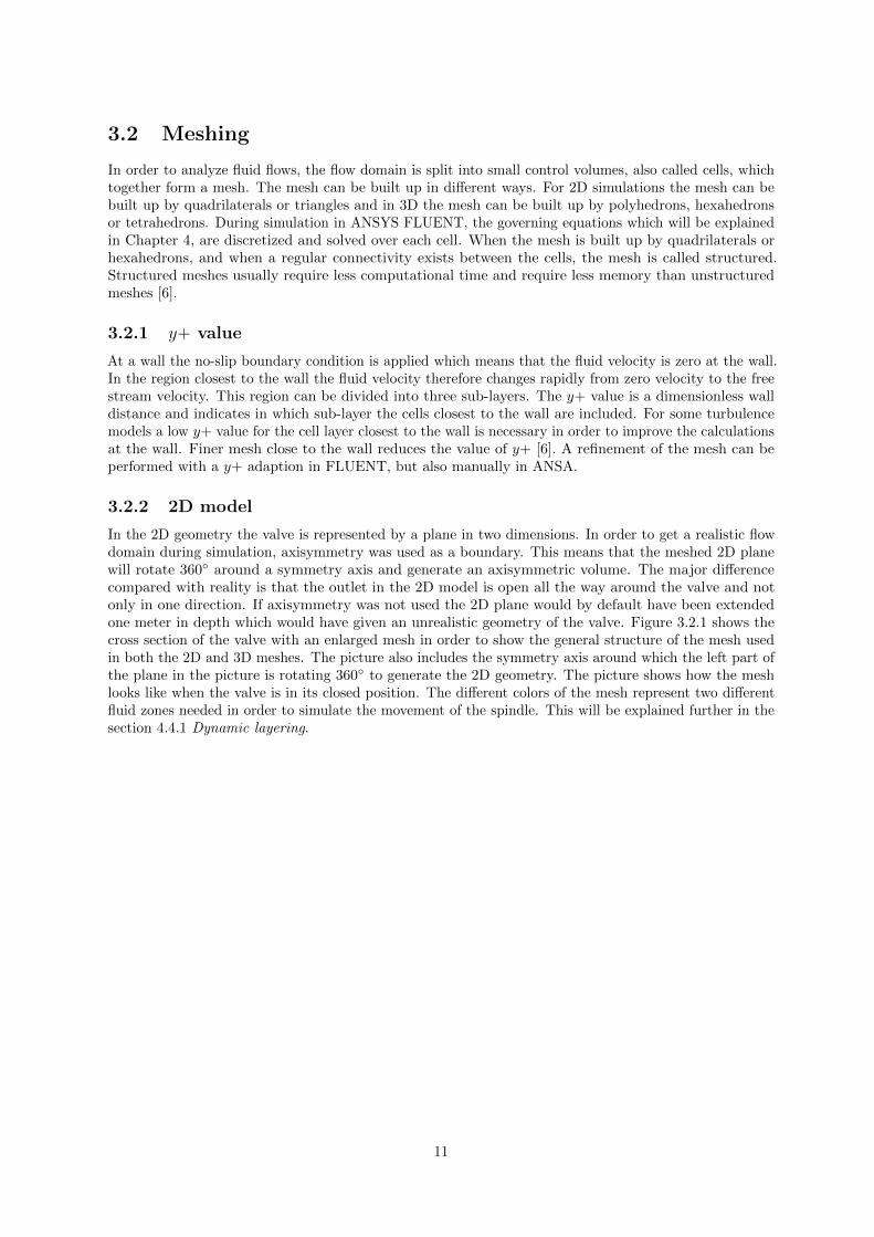
In the 2D geometry the valve is represented by a plane in two dimensions. In order to get a realistic flowdomain during simulation, axisymmetry was used as a boundary. This means that the meshed 2D planewill rotate 360◦ around a symmetry axis and generate an axisymmetric volume. The major differencecompared with reality is that the outlet in the 2D model is open all the way around the valve and notonly in one direction. If axisymmetry was not used the 2D plane would by default have been extendedone meter in depth which would have given an unrealistic geometry of the valve. Figure 3.2.1 shows thecross section of the valve with an enlarged mesh in order to show the general structure of the mesh usedin both the 2D and 3D meshes. The picture also includes the symmetry axis around which the left part ofthe plane in the picture is rotating 360◦ to generate the 2D geometry. The picture shows how the meshlooks like when the valve is in its closed position. The different colors of the mesh represent two differentfluid zones needed in order to simulate the movement of the spindle. This will be explained further in thesection 4.4.1 Dynamic layering.

11

Figure 3.2.1: Cross section of the valve showing the general structure of the mesh used in both the 2D and3D models. The left part of the picture corresponds to the meshed 2D plane which is rotated 360◦ aroundthe symmetry axis.

12

3.2.3 3D model

The 3D geometry is more realistic than the 2D axisymmetric geometry since the valve geometry is createdin three dimensions. In order to reduce the computational time in the 3D simulations mirror symmetry isused. This means that the geometry is cut in half along the cross-sectional plane seen in Figure 3.2.1, andthe number of cells in the mesh is therefore also reduced by half. The cross-sectional plane was chosen tobe the mirror symmetry boundary. This type of boundary implies that no net transport is allowed acrossthe symmetry plane [6]. Figure 3.2.2 shows the volume mesh around the spindle at its closed position andFigure 3.2.3 shows a close-up of the critical area below the spindle, where the fluid flow abruptly changesdirection during discharge. The reason why four layers of mesh are present in the closed valve positionis that a mesh has to exist beneath the spindle in order to simulate the movement of the spindle withdynamic layering. This will be explained further in the section 4.4.1 Dynamic layering and in the section6.1 Initial valve opening of 5 %.

Figure 3.2.2: The 3D mesh around the spindle.

Figure 3.2.3: Close-up of the 3D mesh.

13

4 CFD simulations of a safety relief valveSafety relief valves have been modeled with computational fluid dynamics several times in the past.Amongst others, Xue Guan Song et al. modeled a pressure safety valve in 2D [7] and 3D [8] using ANSYSCFX, and J. Francis et al. [9] modeled a pressure relief valve with incompressible flow and compared itwith experimental data.

The CFD simulations of the safety relief valve in this project were chosen to be performed in ANSYSFLUENT v.13. ANSYS FLUENT is a computer software for modeling of fluid flow, heat transfer andchemical reactions. It predicts the fluid behavior and can handle simulations in complex geometries. Amesh needs to be provided before settings can be chosen and calculations be performed.

The theory in the following chapter is from the ANSYS FLUENT 13 Theory guide [10] and from thebook Computational Fluid Dynamics for Chemical Engineers [6].

4.1 Governing equations

In computational fluid dynamics four governing equations are solved; the continuity equation, themomentum equation, the energy equation and the balance equation for species. The energy equation isnot considered when modeling a safety relief valve since the energy transport in this case is negligible.Also, since only water is flowing through the valve the balance equation for species is not described furtherin this chapter.

4.1.1 Continuity equation

The continuity equation is formulated as

∂ρ

∂t+∂ρUi∂xi

= S(ρ) (4.1.1)

where the first term is the rate of accumulation of mass, the second term is the transport of mass byconvection and the third term the source term. The subscript i ranges from 1 to 3 in 3D.

Since one phase, incompressible flow, i.e. a Mach number < 0.3, is modeled in this project the sourceterm and the accumulation term can be excluded which results in the equation

∂Ui∂xi

= 0 (4.1.2)

As mentioned in Chapter 3, the 2D model has an axisymmetric boundary. The continuity equation can inthis case be written as

∂Ux∂x

+∂Ur∂r

+Urr

= 0 (4.1.3)

4.1.2 Momentum equation

The momentum equation, also known as the Navier-Stokes equation, is written as

∂Ui∂t

+ Uj∂Ui∂xj

= −1

ρ

∂P

∂xi+

1

ρ

∂τji∂xj

+ gi (4.1.4)

where the first term on the left-hand side describes the accumulation of momentum and the second termdescribes the convective acceleration. On the right-hand side the terms describe the pressure forces, shearforces and gravity force [2].

For incompressible flows the density, ρ, and the molecular viscosity, µ, are constant. Therefore, thekinematic viscosity, ν = µ/ρ, is also constant. By combining equation (4.1.4) and (2.3.6) the momentumequation can be written as

∂Ui∂t

+ Uj∂Ui∂xj

= −1

ρ

∂P

∂xi+ ν

∂2Ui∂xj∂xj

+ gi (4.1.5)

14

This equation can also be rewritten for the 2D model with axisymmetric boundary. The axial and radialmomentum equations are in this case formulated as

∂Ux∂t

+1

r

∂(rUxUx)

∂x+

1

r

∂(rUrUx)

∂r=

−1

ρ

∂P

∂x+

1

ρ

1

r

∂

∂x

[rµ

(2∂Ux∂x− 2

3

(∂Ux∂x

+∂Ur∂r

+Urr

))]+ (4.1.6)

1

ρ

1

r

∂

∂r

[rµ

(∂Ux∂r

+∂Ur∂x

)]

∂Ur∂t

+1

r

∂(rUxUr)

∂x+

1

r

∂(rUrUr)

∂r=

−1

ρ

∂P

∂r+

1

ρ

1

r

∂

∂r

[rµ

(2∂Ur∂r− 2

3

(∂Ux∂x

+∂Ur∂r

+Urr

))]+ (4.1.7)

1

ρ

1

r

∂

∂r

[rµ

(∂Ur∂x

+∂Ux∂r

)]− 2µ

Urr2

+2

3

µ

r

(∂Ux∂x

+∂Ur∂r

+Urr

)+ ρ

U2z

r

4.2 Modeling of turbulent flow

It is assumed that the flow through the valve in this project is turbulent since high fluid velocities areachieved when the valve is discharging. A turbulent flow can be solved firstly by decomposing the velocitiesand pressure by using Reynolds decomposition and then combine it with the Navier-Stokes equation(4.1.5). The decomposition means that the variables are split into a mean and a fluctuating part, seeequation (4.2.1) and (4.2.2).

Ui = 〈Ui〉+ ui (4.2.1)

P = 〈P 〉+ p (4.2.2)

The momentum equation can then be written as

∂〈Ui〉∂t

+ 〈Uj〉∂〈Ui〉∂xj

= −1

ρ

∂

∂xj

{〈P 〉δij + µ

(∂〈Ui〉∂xj

+∂〈Uj〉∂xi

)− ρ〈uiuj〉

}(4.2.3)

which is also called Reynolds Average Navier-Stokes (RANS) equation. The δij is the Kronecker delta.The term −ρ〈uiuj〉 in equation (4.2.3) describes the transfer of momentum by turbulence and is

referred to as Reynolds stresses, τT,ij , where i and j range from 1 to 3 in 3D simulations. This term is asecond order tensor and therefore consists of nine terms. However, since it is symmetric it only has sixunknown terms that need to be modeled.

Boussinesq proposed that the Reynolds stresses can be assumed to be proportional to the mean velocitygradients. In his equation the turbulence is modeled as a diffusive process by using a turbulent viscosity,νT , which is comparable with molecular viscosity.

τT,ijρ

= −〈uiuj〉 = νT

(∂〈Ui〉∂xj

∂〈Uj〉∂xi

)− 2

3kδij (4.2.4)

The Boussinesq approximation, equation (4.2.4), is based on the assumptions that the turbulenceis isotropic and that there is a local equilibrium between stress and strain. The turbulent viscosity isunknown but can be estimated with turbulence models. By combining equation (4.2.3) and (4.2.4) thefollowing equation is obtained

∂〈Ui〉∂t

+ 〈Uj〉∂〈Ui〉∂xj

= −1

ρ

∂〈P 〉∂xi

− 2

3

∂k

∂xi+

∂

∂xj

[(ν + νT )

(∂〈Ui〉∂xj

+∂〈Uj〉∂xi

)](4.2.5)

15

where the turbulent kinetic energy, k, is defined as

k =1

2〈uiui〉 (4.2.6)

Turbulence models that are based on the RANS-equation and the Boussinesq approximation consist ofa set of equations that determine the turbulent viscosity, which is proportional to the turbulent velocity,u, and the turbulent length scale, l, see equation (4.2.7).

νT = Cvul (4.2.7)

Cv is a proportionality constant. The turbulent viscosity can be estimated with models consisting of zero,one, two or more equations. The two-equation models are frequently used in the general-purpose flowsimulations since the turbulent velocity and length scales are calculated independently. The realizablek − ε model and the SST k − ω model described below, both belong to the two-equation category. Theturbulent velocity can be calculated by solving the transport equations for the kinetic energy, k, andthe length scale can be estimated with transport equations for, amongst others, the energy dissipationrate, ε, or the specific dissipation, ω. The following equations describe the relationships between theturbulent velocity and kinetic energy, and between the length scale and energy dissipation rate and specificdissipation;

u = k1/2 l =k3/2

εl =

√k

ω(4.2.8)

4.2.1 Realizable k − ε model

In the realizable k − ε model the turbulent viscosity is expressed with the turbulent kinetic energy, k, andthe dissipation rate, ε.

νT = Cvul = Cµk2

ε(4.2.9)

The variable Cµ is expressed as

Cµ =1

A0 +ASkU∗

ε

(4.2.10)

where A0, AS and U∗ are model constants.The following two equations are the transport equations for k and ε. The different terms are described

below each equation.

∂k

∂t+ 〈Uj〉

∂k

∂xj= νT

[(∂〈Uj〉∂xj

+∂〈Uj〉∂xj

)∂〈Uj〉∂xj

]− ε+

∂

∂xj

[(ν +

νTσk

)∂k

∂xj

](4.2.11)

The physical interpretation of the terms from left to right are:1. Accumulation of k2. Convection of k by the mean velocity3. Production of k4. Dissipation of k5. The effective diffusivity of k

∂ε

∂t+ 〈Uj〉

∂ε

∂xj=

∂

∂xj

[(ν +

νTσε

)∂ε

∂xj

]+ C1Sε− C2

ε2

k +√νε

(4.2.12)

The physical interpretation of the terms from left to right are:1. Accumulation of ε2. Convection of ε by the mean velocity3. Diffusion of ε4. Production of ε5. Dissipation of ε

C1, C2, σk and σε are model constants.

16

The realizable k − ε model is similar to the standard k − ε model. The transport equation for kineticenergy is the same in both models, except for the model constants. However, the transport equationfor the dissipation energy is modified in the realizable model compared to the standard model and theequation for the turbulent viscosity (4.2.9) includes a variable Cµ which prevents the normal stresses frombecoming negative.

The realizable k − ε turbulence model gives a better prediction of swirling flows and flow separationsthan the standard k − ε turbulence model.

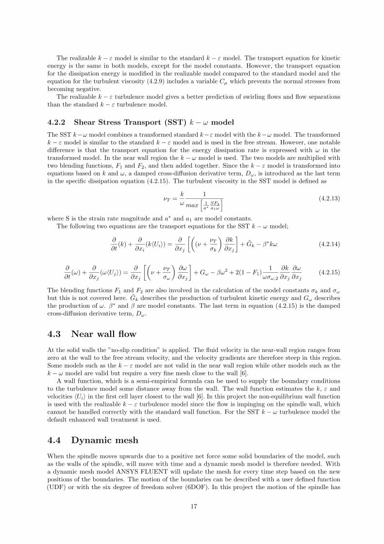
4.2.2 Shear Stress Transport (SST) k − ω model

The SST k−ω model combines a transformed standard k−ε model with the k−ω model. The transformedk − ε model is similar to the standard k − ε model and is used in the free stream. However, one notabledifference is that the transport equation for the energy dissipation rate is expressed with ω in thetransformed model. In the near wall region the k − ω model is used. The two models are multiplied withtwo blending functions, F1 and F2, and then added together. Since the k − ε model is transformed intoequations based on k and ω, a damped cross-diffusion derivative term, Dω, is introduced as the last termin the specific dissipation equation (4.2.15). The turbulent viscosity in the SST model is defined as

νT =k

ω

1

max[

1a∗

SF2

a1ω

] (4.2.13)

where S is the strain rate magnitude and a∗ and a1 are model constants.The following two equations are the transport equations for the SST k − ω model;

∂

∂t(k) +

∂

∂xi(k〈Ui〉) =

∂

∂xj

[((ν +

νTσk

)∂k

∂xj

]+ Gk − β∗kω (4.2.14)

∂

∂t(ω) +

∂

∂xj(ω〈Uj〉) =

∂

∂xj

[(ν +

νTσω

)∂ω

∂xj

]+Gω − βω2 + 2(1− F1)

1

ωσω,2

∂k

∂xj

∂ω

∂xj(4.2.15)

The blending functions F1 and F2 are also involved in the calculation of the model constants σk and σωbut this is not covered here. Gk describes the production of turbulent kinetic energy and Gω describesthe production of ω. β∗ and β are model constants. The last term in equation (4.2.15) is the dampedcross-diffusion derivative term, Dω.

4.3 Near wall flow

At the solid walls the ”no-slip condition” is applied. The fluid velocity in the near-wall region ranges fromzero at the wall to the free stream velocity, and the velocity gradients are therefore steep in this region.Some models such as the k − ε model are not valid in the near wall region while other models such as thek − ω model are valid but require a very fine mesh close to the wall [6].

A wall function, which is a semi-empirical formula can be used to supply the boundary conditionsto the turbulence model some distance away from the wall. The wall function estimates the k, ε andvelocities 〈Ui〉 in the first cell layer closest to the wall [6]. In this project the non-equilibrium wall functionis used with the realizable k − ε turbulence model since the flow is impinging on the spindle wall, whichcannot be handled correctly with the standard wall function. For the SST k − ω turbulence model thedefault enhanced wall treatment is used.

4.4 Dynamic mesh

When the spindle moves upwards due to a positive net force some solid boundaries of the model, suchas the walls of the spindle, will move with time and a dynamic mesh model is therefore needed. Witha dynamic mesh model ANSYS FLUENT will update the mesh for every time step based on the newpositions of the boundaries. The motion of the boundaries can be described with a user defined function(UDF) or with the six degree of freedom solver (6DOF). In this project the motion of the spindle has

17

been described with a UDF, which will be explained in section 4.4.2 User Defined Function. FLUENThas three methods for updating the mesh [10];

• Smoothing methods

• Remeshing methods

• Dynamic layering

The smoothing methods include spring-based smoothing, diffusion-based smoothing, Laplaciansmoothing and boundary smoothing. These methods can only be used if the boundary displacement,relative to the cell size, is small since no new cells will be added during the transient simulation. Insteadthe original cells in the mesh are stretched out or compressed since the edges between two mesh nodesbehave like springs.

The remeshing methods are used if the boundary displacement is large relative to the cell size. Cellsthat do not satisfy the skewness criterion are remeshed during the transient simulation. This methodworks on most types of problems. However, it requires large computational power.

Dynamic layering adds or removes layers of cells which are adjacent to the extending boundary. Thismethod can only be used if the mesh is structured and consists of quadrilateral, hexahedral or wedgedmesh.

These three methods can be used separately or combined.

4.4.1 Dynamic layering

In this project the dynamic layering method is used. To achieve a mesh of good quality during thetransient simulation it is practical to divide the fluid domain into two parts, see Figure 4.4.1. The largestpart of the fluid domain is called stationary zone. In this part no change in the volume mesh takes placeduring the transient simulation. The part around the spindle is called the rigid zone and moves along thespindle with the same speed. The dynamic layering takes place within this zone and a structured mesh isa necessity.

Figure 4.4.1: Important parts for the dynamic layering method.

18

When the spindle moves upwards, layers below the spindle in the rigid zone will expand at the extendingboundary and then split according to;

hmin > (1 + as)hideal,e (4.4.1)

where hmin is the minimum cell height of a cell layer, hideal,e is the value of ideal height of the new celllayer beneath the spindle and as is the layer split factor. At the collapsing boundary at the top of therigid zone, the layers are compressed until they collapse according to;

hmin < achideal,c (4.4.2)

where ac is the layer collapse factor and hideal,c is the ideal height of the new cell layer above the spindle.Between the rigid zone and the stationary zone, and within the stationary zone non-conformal interfaces

are present, see Figure 4.4.1. They allow the mesh on each side of the interface to be different. This isnecessary in this project because of two reasons. Firstly, an interface is needed on each side of the spindlesince the structured mesh around the spindle will change with time while the mesh on the other sideof the interface stays unchanged. Secondly, the interfaces at the outlet and the inlet allow the mesh inthese regions to be larger than the mesh around the spindle and consequently reduces the mesh density.However, the difference in mesh size on each side of the interface may not be too large since this couldresult in incorrect calculations. The different meshes on each side of the interfaces can also be observed inFigure 3.2.1.

The dynamic layering method requires that at least one cell layer is present at the extending boundaryin the beginning of the simulation from which next layers can be formed. The safety relief valve cantherefore not be modeled from a completely closed starting position. The valve is therefore chosen to be5 % open from the beginning of the simulation.

4.4.2 User Defined Function

A UDF is written in C programming language and allows the simulations in ANSYS FLUENT to becustomized. The customized settings are defined with DEFINE macros. In this project the UDF is usedto define the movement of the spindle based on the forces acting on it, to define the inlet boundaryconditions and to write data to a text document.

The UDF consists of three different types of macros, and in total six macros are used. In the first type,DEFINE ADJUST, the hydraulic forces on the spindle are calculated by taking the sum of the product ofthe pressure in each cell and the cell area. These calculations are executed at every iteration before thetransport equations are solved. A separate DEFINE ADJUST macro calculates the mass flow throughthe valve.

The second type, DEFINE EXECUTE AT END, consists of three macros. The calculations in thesemacros take place at the end of each time step. The first macro calculates the movement of the spindle,in other words the actual lift, which is also necessary to calculate the spring force. The second macrocalculates the forces acting on the spindle, except from the hydraulic force which was calculated inDEFINE ADJUST. The velocity of the spindle is calculated from the achieved forces with equation (2.3.2).The third macro writes a text document which includes the values of velocity of the spindle, hydraulicforce, spring force, net force, time elapsed, the lift of the spindle, the total pressure at the inlet and themass flow for every time step of the simulation.

The third type of macro, DEFINE CG MOTION, is used to specify the spindle movement. Both linearand angular velocities can be returned to FLUENT through this macro. However, in this project the spindlemovement is linear and the angular velocity is therefore set to zero. In this UDF the velocity of the spindleis calculated in the macro DEFINE EXECUTE AT END and then through DEFINE CG MOTION thevelocity is returned to FLUENT.

The UDF for the 2D and the 3D simulations are similar. However, the calculations of the hydraulicforces in the 3D case are exact, while in the 2D case the spindle is divided into four parts where theaverage pressure is calculated in each part and thereafter multiplied with the total area of the part.

The UDFs used in the 2D and 3D simulations are attached in Appendix A.

19

5 One-dimensional simulations of a safetyrelief valve

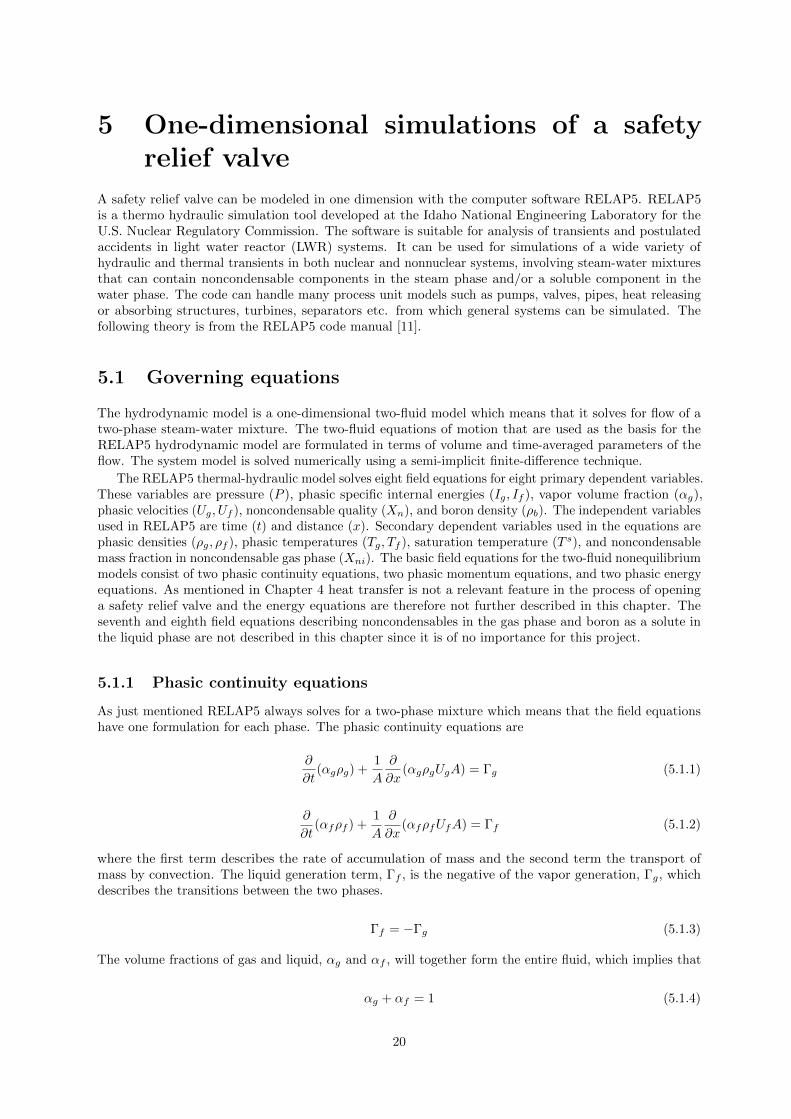
A safety relief valve can be modeled in one dimension with the computer software RELAP5. RELAP5is a thermo hydraulic simulation tool developed at the Idaho National Engineering Laboratory for theU.S. Nuclear Regulatory Commission. The software is suitable for analysis of transients and postulatedaccidents in light water reactor (LWR) systems. It can be used for simulations of a wide variety ofhydraulic and thermal transients in both nuclear and nonnuclear systems, involving steam-water mixturesthat can contain noncondensable components in the steam phase and/or a soluble component in thewater phase. The code can handle many process unit models such as pumps, valves, pipes, heat releasingor absorbing structures, turbines, separators etc. from which general systems can be simulated. Thefollowing theory is from the RELAP5 code manual [11].

5.1 Governing equations

The hydrodynamic model is a one-dimensional two-fluid model which means that it solves for flow of atwo-phase steam-water mixture. The two-fluid equations of motion that are used as the basis for theRELAP5 hydrodynamic model are formulated in terms of volume and time-averaged parameters of theflow. The system model is solved numerically using a semi-implicit finite-difference technique.

The RELAP5 thermal-hydraulic model solves eight field equations for eight primary dependent variables.These variables are pressure (P ), phasic specific internal energies (Ig, If ), vapor volume fraction (αg),phasic velocities (Ug, Uf ), noncondensable quality (Xn), and boron density (ρb). The independent variablesused in RELAP5 are time (t) and distance (x). Secondary dependent variables used in the equations arephasic densities (ρg, ρf ), phasic temperatures (Tg, Tf ), saturation temperature (T s), and noncondensablemass fraction in noncondensable gas phase (Xni). The basic field equations for the two-fluid nonequilibriummodels consist of two phasic continuity equations, two phasic momentum equations, and two phasic energyequations. As mentioned in Chapter 4 heat transfer is not a relevant feature in the process of openinga safety relief valve and the energy equations are therefore not further described in this chapter. Theseventh and eighth field equations describing noncondensables in the gas phase and boron as a solute inthe liquid phase are not described in this chapter since it is of no importance for this project.

5.1.1 Phasic continuity equations

As just mentioned RELAP5 always solves for a two-phase mixture which means that the field equationshave one formulation for each phase. The phasic continuity equations are

∂

∂t(αgρg) +

1

A

∂

∂x(αgρgUgA) = Γg (5.1.1)

∂

∂t(αfρf ) +

1

A

∂

∂x(αfρfUfA) = Γf (5.1.2)

where the first term describes the rate of accumulation of mass and the second term the transport ofmass by convection. The liquid generation term, Γf , is the negative of the vapor generation, Γg, whichdescribes the transitions between the two phases.

Γf = −Γg (5.1.3)

The volume fractions of gas and liquid, αg and αf , will together form the entire fluid, which implies that

αg + αf = 1 (5.1.4)

20

5.1.2 Phasic momentum equations

The momentum formulations used in RELAP5 are simplified, which is not the case for the formulations ofmass and energy conservation, since momentum effects are secondary to mass and energy conservation inreactor safety analysis. A less exact formulation of the momentum is therefore acceptable, especially sincenuclear reactor flows are dominated by large sources and sinks of momentum. Examples of simplificationsof the momentum equations are that the Reynolds and phasic viscous stresses are neglected and thephasic pressures are assumed to be equal. The phasic momentum equations for the gas and liquid phaserespectively are

∂Ug∂t

+1

2

∂U2g

∂x= − 1

ρg

∂P

∂x+Bx − FWG(Ug) +

Γgαgρg

(UgI − Ug)−

FIG(Ug − Uf )− Cαfρmρg

[∂(Ug − Uf )

∂t+ Uf

∂Ug∂x− Ug

∂Uf∂x

] (5.1.5)

∂Uf∂t

+1

2

∂U2f

∂x= − 1

ρf

∂P

∂x+Bx − FWF (Uf )− Γf

αfρf(UfI − Uf )−

FIF (Uf − Ug)− Cαgρmρf

[∂(Uf − Ug)

∂t+ Ug

∂Uf∂x− Uf

∂Ug∂x

] (5.1.6)

The terms on the left-hand sides in the momentum equations describe the accumulation of momentumand convective acceleration respectively. The force terms on the right-hand sides in the momentumequations are the pressure gradient, the body force due to gravity, wall friction, momentum transferdue to interface mass transfer, interface frictional drag, and force due to virtual mass. The last threeterms are included in the RELAP5 model since the model solves for the two phases, gas and liquid,simultaneously and therefore must take multiphase terms into consideration. This is different from themomentum formulation used in FLUENT, see equation (4.1.4). The formulation in FLUENT does notinclude the multiphase terms since FLUENT has other equations which separately describe multiphaseinteractions. But since only one phase is present in the safety relief valve model the multiphase interactionsare disregarded in FLUENT. The terms FWG and FWF in equations (5.1.5) and (5.1.6) are the vaporand liquid wall drag coefficients respectively. FIG and FIF are the interface drag coefficients for gasand liquid respectively. C is the coefficient of virtual mass and UI is the velocity at the interface formultiphase calculations.

5.2 Modeling of valves in RELAP5

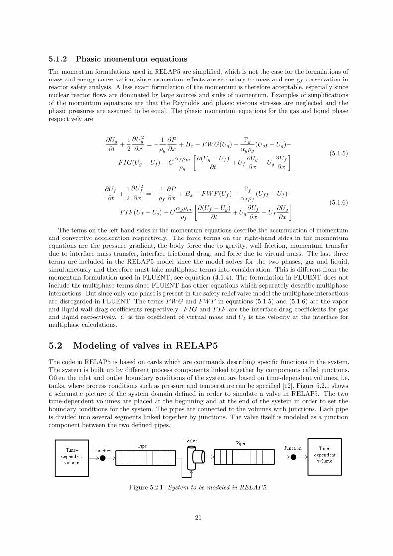
The code in RELAP5 is based on cards which are commands describing specific functions in the system.The system is built up by different process components linked together by components called junctions.Often the inlet and outlet boundary conditions of the system are based on time-dependent volumes, i.e.tanks, where process conditions such as pressure and temperature can be specified [12]. Figure 5.2.1 showsa schematic picture of the system domain defined in order to simulate a valve in RELAP5. The twotime-dependent volumes are placed at the beginning and at the end of the system in order to set theboundary conditions for the system. The pipes are connected to the volumes with junctions. Each pipeis divided into several segments linked together by junctions. The valve itself is modeled as a junctioncomponent between the two defined pipes.

Figure 5.2.1: System to be modeled in RELAP5.

21

Since the valve is modeled as a junction component the user has the possibility to vary the junctionflow area as a function of time and/or hydrodynamic properties. Valve action is modeled explicitly andtherefore lags the hydrodynamic calculational results by one time step.

Valves are classified as quasi-steady models in RELAP5, which means that some phenomena areconsidered as steady state whereas others are considered as transient during the same simulation. Severalvalve models are available in RELAP5. The models can be classified into two categories; valves that openor close instantly and valves that open or close gradually. The first category includes trip valves and checkvalves, whereas the second category includes the inertial swing check valves, motor valves, servo valves,and relief valves [11]. In this project the motor and servo valve models are investigated.

5.2.1 Motor and servo valve models

There are some similarities between the motor and the servo valve models. Both valve models use anormalized stem position which means that the position of the spindle ranges between 0.0 for the closedposition and 1.0 for the fully open position. For both valves a general table can be used to describe thenormalized flow area for a given normalized stem position. If the general table is not used, the normalizedflow area is set to equal the normalized stem position.

The flow through both valve types is determined by the flow area and the energy losses. There aretwo models available in RELAP5 to calculate the losses; the abrupt area change model and the smootharea change model. In the abrupt area change model the valve flow area is treated as the orifice area. Inthis project that means that the area between the inlet and the outlet of the valve changes abruptly, seeFigure 5.2.2. The kinetic form losses are calculated with respect to the valve area by RELAP5.

Figure 5.2.2: Illustration of how the valve area changes with the abrupt area change model.

The smooth area change model requires that a Cv table is included which contains forward and reverseflow coefficients as a function of normalized valve area or normalized stem position. The Cv table isspecified by the user and the flow coefficients are further converted to energy loss coefficients, K, through

K = 2A2valve

C2vρo

=∆P

ρU2/2(5.2.1)

where ρo is the density of water at 288.71 K.The main difference between the two valve models is how the actual opening and closing features of

the valve are controlled.

Motor valve modelWith the motor valve model the opening and closing of the valve are controlled by two trips. The trips

describe at what conditions the valve should be opened or closed, for example during a specified timeinterval in the simulation or in a specific pressure interval. A constant rate parameter is used in order tocontrol the speed at which the valve area changes and hence the positioning of the valve. The constantrate parameter can also control the valve stem position in combination with a general table which relatesthe stem position to a valve flow area.

Servo valve modelWith the servo valve model the opening and closing processes of the valve are controlled with controlvariables. The control variables allow the user to specify what calculations that should be performedduring simulation, which makes the servo valve model the most flexible model to use when simulating

22

a valve in RELAP5. Variables such as pressure, mass flow, density, temperature etc. can be accessedthrough the control variables. In the servo valve model in this project the control variables are used inorder to calculate the forces acting on the spindle. These calculations are very similar to the calculationsin the UDF which was used in FLUENT. The following forces are included in the servo valve model; thegravity force, the spring force and the total hydraulic force.

Ftot = Fg + Fs + Fh (5.2.2)

Fg = mg (5.2.3)

Fs = −k(xo + h) (5.2.4)

The equation explaining the total hydraulic force, Fh, is however unknown. In RELAP5 this force cannotbe calculated by multiplying the local pressure at the spindle with the surface area of the spindle, asin FLUENT, since the valve in RELAP5 is a 1D model which lacks details of the geometry. Insteadthe hydraulic force needs to expressed with the inlet and/or the outlet pressure and maybe some moreunknown terms. When all the forces acting on the spindle are known the velocity of the spindle, v, can becalculated according to;

v − vold =

∫F

mdt =

1

2m(F + Fold)∆t (5.2.5)

and the lift of the spindle, h, is determined with;

h− hold =

∫v dt =

1

2(v + vold)∆t (5.2.6)

These two equations were obtained by approximating the integrals according to the trapetzoidal method.

5.3 Force calculations

The opening of a valve generates forces acting on the pipe systems. According to Newton’s second law theforce in a pipe segment is equal to the change of total momentum within the fluid, see equation (5.3.1).

F =d

dt

∫ L

0

mdL (5.3.1)

where L is the total pipe length. In RELAP5 this integral can be solved by discretization where the pipelength is subdivided into smaller segments.∫ L

0

mdL ≈n∑i=1

mi∆L (5.3.2)

where n is the number of junctions within the pipe, ∆L describes the distance between the center pointsof each segment and mi is the mass flow through each junction within the pipe. In this project the forcesin the pipes are calculated according to equation (5.3.3). For the first and last element in the pipes onlyhalf of the element length is used in order to include the first and last halves of the end segments in theforce calculations.

F =d

dt

(m1

∆L

2+

n−1∑i=2

mi∆L+ mn∆L

2

)(5.3.3)

23

6 Settings used in the CFD and RELAP5simulations

This chapter summarizes important information and settings for the CFD and RELAP5 simulations ofthe safety relief valve.

6.1 Initial valve opening of 5 %

The geometries of the 2D and 3D CFD models were created according to the dimensions mentioned inChapter 3. In order to use the dynamic layering method at least one layer of cells is needed initiallybeneath the spindle. This means that the valve cannot be completely closed at the initial position.Furthermore, if the valve is completely closed, the mesh between the inlet and the valve body wouldbe disconnected. This would cause numerical difficulties since information cannot be transported in thefluid domain. In this project a start opening of 5 % of maximum opening is used which equals an initialopening of 0.425 mm. One motivation of this choice is that an initial opening of 0.425 mm leaves enoughspace for building four initial layers of mesh beneath the spindle, which is considered as a better startingmesh for simulation of turbulent flow. With a smaller opening the mesh quality would decrease sincefewer mesh layers would exist and the quality of the calculations would decrease.

It has also been observed that a safety relief valve starts to leak fluid before it is about to open [13].Therefore, the assumed initial opening in the model may be a representative assumption of the leakage offluid before the valve starts to open.

6.2 Spring settings

For the spring, two constants were specified; the spring constant k and the initial tension force F0, seeequation (2.3.8). The value of k was chosen as a mean value of measured k values during a series of threeexperiments conducted by the valve manufacturer. The value of F0 was calculated as the force acting onthe bottom surface of the spindle at completely closed position at the set pressure 31 bar(g). The usedconstants are

k = 722150 N/m2

F0 = 7126 N

6.3 Mass of spindle

The mass of importance in the valve model is the mass of the spindle which includes the disc, the shroudand the rod. The total moving mass is

m = 3.1928 kg

The material of the spindle was given in the original drawing which means that the density of the spindlewas known. The total volume of the spindle was assumed to be equal to the volumes of the disc, theshroud and the rod using dimensions from the original drawing. Other structures might therefore belongto the spindle volume which are not included in this mass calculation which means that the used massmight be underestimated.

24

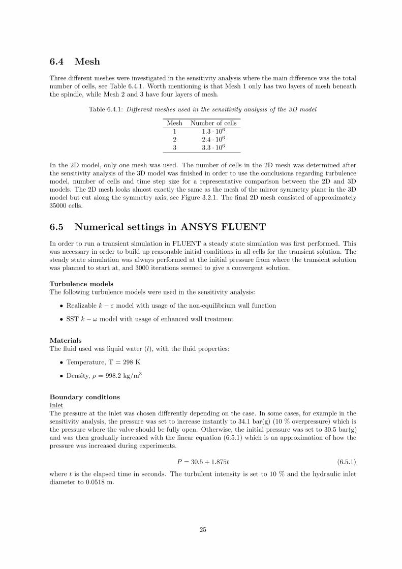
6.4 Mesh

Three different meshes were investigated in the sensitivity analysis where the main difference was the totalnumber of cells, see Table 6.4.1. Worth mentioning is that Mesh 1 only has two layers of mesh beneaththe spindle, while Mesh 2 and 3 have four layers of mesh.

Table 6.4.1: Different meshes used in the sensitivity analysis of the 3D model

Mesh Number of cells1 1.3 · 106

2 2.4 · 106

3 3.3 · 106

In the 2D model, only one mesh was used. The number of cells in the 2D mesh was determined afterthe sensitivity analysis of the 3D model was finished in order to use the conclusions regarding turbulencemodel, number of cells and time step size for a representative comparison between the 2D and 3Dmodels. The 2D mesh looks almost exactly the same as the mesh of the mirror symmetry plane in the 3Dmodel but cut along the symmetry axis, see Figure 3.2.1. The final 2D mesh consisted of approximately35000 cells.

6.5 Numerical settings in ANSYS FLUENT

In order to run a transient simulation in FLUENT a steady state simulation was first performed. Thiswas necessary in order to build up reasonable initial conditions in all cells for the transient solution. Thesteady state simulation was always performed at the initial pressure from where the transient solutionwas planned to start at, and 3000 iterations seemed to give a convergent solution.

Turbulence modelsThe following turbulence models were used in the sensitivity analysis:

• Realizable k − ε model with usage of the non-equilibrium wall function

• SST k − ω model with usage of enhanced wall treatment

MaterialsThe fluid used was liquid water (l), with the fluid properties:

• Temperature, T = 298 K

• Density, ρ = 998.2 kg/m3

Boundary conditionsInletThe pressure at the inlet was chosen differently depending on the case. In some cases, for example in thesensitivity analysis, the pressure was set to increase instantly to 34.1 bar(g) (10 % overpressure) which isthe pressure where the valve should be fully open. Otherwise, the initial pressure was set to 30.5 bar(g)and was then gradually increased with the linear equation (6.5.1) which is an approximation of how thepressure was increased during experiments.

P = 30.5 + 1.875t (6.5.1)

where t is the elapsed time in seconds. The turbulent intensity is set to 10 % and the hydraulic inletdiameter to 0.0518 m.

25

OutletThe static pressure at the outlet was set to 0 bar(g). The turbulent intensity is set to 10 % and thehydraulic outlet diameter to 0.1 m.

Dynamic meshUnder the Dynamic Mesh tab in FLUENT the Layering method is chosen and all surfaces and fluidregions inside the rigid zone, see Figure 4.4.1, have to be created by denoting them as rigid or stationarydepending on their function in the movement of the spindle. The boundaries where the mesh is growingfrom and where it is collapsing are denoted as stationary. Following settings were used in the dynamicmesh;

• hideal,e is different for the investigated meshes since different number of cell layers beneath thespindle were used. For Mesh 1 where two layers of cells were initially existing, hideal,e was 0.2 mm.For Mesh 2 and 3, hideal,e was 0.1 mm since four layers of mesh were initially existing.

• hideal,c had the same value, 0.6 mm, for all three meshes since there was no difference in mesh sizein that region between the investigated meshes.

• In this project the values of as and ac were constant for all simulations, as =0.4 and ac=0.2.

Solution methods

• The scheme for pressure velocity coupling is chosen to be coupled.

• During the steady state simulations, second order upwind was used for the momentum. First orderupwind was used for the turbulent kinetic energy and specific dissipation rate.

• During the transient simulations, second order upwind was always used for momentum, turbulentkinetic energy and specific dissipation rate.

Solution controls

• Courant number of 20 was always used.

• Explicit relaxation factor of momentum: 0.25

• Explicit relaxation factor of pressure: 0.25

MonitorsFor the steady state simulations, no residuals have been used. For the transient simulations all residualshad the default value of 10−3 except from the continuity which was set to 10−5.

Run calculation

• During steady state simulations 3000 iterations were used.

• During transient simulations the number of time steps varied depending on the case. In the sensitivityanalysis three different time step sizes were investigated; 0.1, 0.25 and 0.5 ms. During the simulationwhere the pressure was gradually increased from 30.5 bar(g) until the valve was fully open a timestep size of 1 ms was used.

6.6 Numerical settings in RELAP5

The time dependent volumes had a volume of 50 m3 and the used fluid was water with a temperature of298 K. The pipes were divided into 20 segments with a length of 0.1 m. The total length of the two pipeswas therefore 2 meters each.

26

Valve models

• For the currently used motor valve model an opening time of 1 ms was used and the inlet pressurewas set to 34.1 bar(g).

• In the modified motor valve model the opening time was changed to 41 ms and a Cv table wasincluded describing forward and reverse flow coefficients as a function of normalized stem position.The inlet pressure was set to 34.1 bar(g).

• In the servo valve model control variables were written for all relations necessary for the simulationof the valve in this project. The inlet pressure was gradually increased, with equation (6.5.1), from30.5 bar(g) until the valve was fully open.

The code for the currently used and the modified motor valve models are attached in Appendix B and thecode for the servo valve model is attached in Appendix C.

27

7 Sensitivity analysis of the CFD simulationsA sensitivity analysis was performed in order to investigate if and to which extent different mesh densities,turbulence models and time step sizes influence the results of the CFD simulations. The 3D geometrywas used for the analysis and the inlet pressure was instantly increased to 34.1 bar(g). The conclusionsfrom the investigation formed the basis of the settings used in the main simulations. The results of thesensitivity analysis are presented in this chapter.

7.1 Mesh density

Three different mesh densities were investigated; 1.3, 2.4 and 3.3 million cells. The results are illustratedin Figures 7.1.1 and 7.1.2. It can be observed in Figure 7.1.1 a) and b) that the overall behavior of thesafety relief valve is the same for all three mesh densities. However, the 1.3 million mesh differs the mostwith a shorter opening time of the valve and a higher velocity of the spindle. The difference from the othertwo meshes might be due to that only two layers of initial mesh exist beneath the spindle in the 1.3 millionmesh at the starting position. The mesh might not be fine enough in order for the transport equations tobe solved correctly. Another reason for the deviation might be that the difference in mesh size on bothsides of the interfaces in the 1.3 million mesh is large, which might cause incorrect calculations over theinterfaces.

The difference between the 2.4 and 3.3 million meshes is insignificant, both in opening times of thevalve and velocities of the spindle. In these meshes four layers of mesh were existing beneath the spindleat the starting position which is an improvement by a factor two compared with the 1.3 million mesh. Themesh quality is better in these two meshes and the meshes at the interfaces are more uniform. Figure 7.1.2shows that there is no difference in opening time between the 2.4 and 3.3 million meshes and the conclusionis that the solution seems to be mesh independent. Further refining of the mesh is not considered asnecessary.

Figure 7.1.1: a) Opening profile of the valve and b) velocity of the spindle, for different mesh densities.

28

Figure 7.1.2: Opening times for the different mesh densities. There is no difference in opening timebetween the 2.4 and 3.3 million meshes.

From these observations the mesh with 3.3 million cells was chosen for the main simulations since afiner mesh should give more accurate results and the computational time was not much longer than forthe mesh with 2.4 million cells.

7.2 Turbulence models and time step sizes

Two different turbulence models were investigated for transient simulation in the sensitivity analysis; theSST k − ω model and the realizable k − ε model. The 3.3 million mesh was used during the investigation.The impact of the different time steps 0.5 ms, 0.25 ms and 0.1 ms, were also investigated for the differentturbulence models during the transient simulations.

The steady state simulations, which are performed at the closed position of the valve, were simulatedwith the SST k−ω model. The transient simulations were then performed with the two different turbulencemodels. This is based on the assumption that when the valve is closed there is almost no mass flowthrough the valve and therefore the choice of turbulence model should not affect the results in the steadystate simulation.

In Figures 7.2.1 and 7.2.2 it can be observed that the safety relief valve opens faster with the SSTmodel. It can also be observed that the opening time of the valve decreases with shorter time step, whichis most distinguishable for the realizable k− ε model. The opening times for the SST model do not changemuch for different time steps, which gives an indication that the SST model seems to be more consistentthan the realizable model. The difference in opening time between the two models is relatively largewith the longest time step, 0.5 ms, where the opening time was 41 ms with the SST model and 53.5 mswith the realizable model. With the shortest time step, 0.1 ms, the opening time was 40.5 ms with theSST model and 45.5 ms with the realizable model. This shows that the time step during the transientsimulation has a large impact on the results.

29

Figure 7.2.1: a) Lift of spindle vs. time for different turbulence models and time steps. b) A close-up ofthe final part of the opening process where the differences are more apparent.

Figure 7.2.2: Opening time of the valve vs. time step in the transient simulations for the differentturbulence models.

In Figure 7.2.3 an even more apparent difference between the two turbulence models can be observed.This figure shows how the velocity of the spindle changes with time. During the first 15 ms of thesimulation the velocity of the spindle for both turbulence models and all time steps is almost equal.However, when the spindle accelerates the second time, differences appear between the models. Thevelocity increases faster with the SST model and the spindle reaches the maximum lift, 8.5 mm, with highvelocity. The velocity increases less with the realizable model and then declines which leads to that thespindle is almost standing still before the maximum lift is reached. In this figure it can also be observedthat the velocity of the spindle reaches higher values with a shorter time step for both models. However,the difference between the time steps within the realizable model is larger than the difference within theSST model which again indicates that the SST model seems to be more consistent.

When these two turbulence models were compared it was observed that the realizable model estimatesa higher turbulence in this valve model than the SST model. This can explain the lower velocity of thespindle when using the realizable model since a higher turbulence results in lower fluid pressure and thuslower hydraulic forces acting on the spindle. Lower hydraulic forces result in lower velocity of the spindle.The difference in turbulence prediction can also be the reason why the largest difference of velocity can beobserved at the end of the simulation since the turbulence increases with the lift of the spindle.

30

Figure 7.2.3: Velocity of spindle vs. time for different turbulence models and time steps.

Since the two models show a different behavior during the opening of the valve, which have beenobserved in Figure 7.2.3, it is impossible to say which of the turbulence models that predicts the realbehavior of the valve. However, the SST k − ω model is chosen for the main simulations because of threereasons:

• The SST model gives the shortest opening times of the valve. When there is an uncertainty withinnuclear engineering the most conservative choice, i.e. the worst case should be chosen. A shorteropening time of a valve creates larger forces on the pipes downstream which is considered as a worstcase scenario and hence the most conservative case.

• The SST model seems to be more consistent than the realizable model. When the time step sizewas decreased the difference between the three simulations using the SST model was small.

• Since there is no large difference between the different time steps with the SST model the largesttime step, 0.5 ms, can be chosen for the main simulations which gives a shorter computational timethan if shorter time steps were used. This is an advantage for the SST model compared with therealizable model where a short time step might have been necessary in order to achieve reasonableresults, and the calculations would have been more time consuming.

31

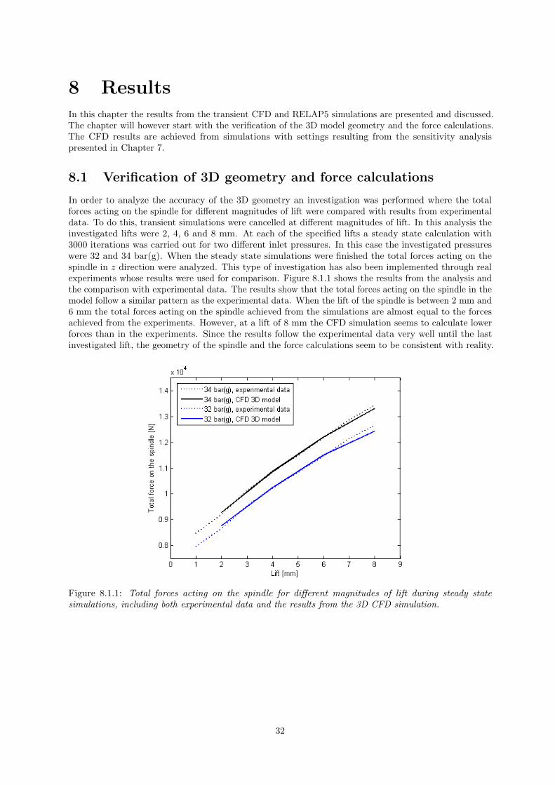
8 ResultsIn this chapter the results from the transient CFD and RELAP5 simulations are presented and discussed.The chapter will however start with the verification of the 3D model geometry and the force calculations.The CFD results are achieved from simulations with settings resulting from the sensitivity analysispresented in Chapter 7.

8.1 Verification of 3D geometry and force calculations

In order to analyze the accuracy of the 3D geometry an investigation was performed where the totalforces acting on the spindle for different magnitudes of lift were compared with results from experimentaldata. To do this, transient simulations were cancelled at different magnitudes of lift. In this analysis theinvestigated lifts were 2, 4, 6 and 8 mm. At each of the specified lifts a steady state calculation with3000 iterations was carried out for two different inlet pressures. In this case the investigated pressureswere 32 and 34 bar(g). When the steady state simulations were finished the total forces acting on thespindle in z direction were analyzed. This type of investigation has also been implemented through realexperiments whose results were used for comparison. Figure 8.1.1 shows the results from the analysis andthe comparison with experimental data. The results show that the total forces acting on the spindle in themodel follow a similar pattern as the experimental data. When the lift of the spindle is between 2 mm and6 mm the total forces acting on the spindle achieved from the simulations are almost equal to the forcesachieved from the experiments. However, at a lift of 8 mm the CFD simulation seems to calculate lowerforces than in the experiments. Since the results follow the experimental data very well until the lastinvestigated lift, the geometry of the spindle and the force calculations seem to be consistent with reality.

Figure 8.1.1: Total forces acting on the spindle for different magnitudes of lift during steady statesimulations, including both experimental data and the results from the 3D CFD simulation.

32

8.2 CFD simulations of the safety relief valve

In this section the results from the transient CFD simulations of the safety relief valve are presented.Firstly, the results from the 3D simulation, where the inlet pressure was instantly increased to 34.1 bar(g),are presented and discussed. This is followed by the results from the corresponding investigation performedwith the 2D model in order to compare the two different models. The last part of the section coversthe simulations where the inlet pressure was gradually increased from 30.5 bar(g) until the valve wascompletely opened. In this part the results from the 2D and 3D simulations are integrated and comparedwith experimental data. Interesting observations and parameter relations are discussed. These relationsare further used in the one-dimensional simulations in RELAP5, whose results are presented in the nextsection.

The results presented for the CFD simulations in 3D, with an instant increase of inlet pressure, areachieved from simulations performed with a mesh consisting of 3.3 million cells, SST k − ω as turbulencemodel and a time step size of 0.5 ms. The results from the corresponding 2D simulations are achievedfrom simulations performed with the same turbulence model, the same time step size but with a meshconsisting of approximately 35000 cells. These settings are based on the results from the sensitivityanalysis. In the simulations where the inlet pressure is gradually increased the time step size is 1 ms butthe other settings mentioned remain the same.

8.2.1 3D model - Instant increase of inlet pressure

Within nuclear engineering conservative settings are of importance in order to analyze worst case scenar-ios. Therefore, the valve features were investigated when the inlet pressure was instantly increased to34.1 bar(g) which is the pressure where the valve should be fully open. The instant increase of inletpressure should give the shortest opening time of the valve which would be the most conservative case.Figure 8.2.1 shows the opening profile of the valve, i.e. the lift of the spindle vs. time when the valve issimulated in 3D. It takes 41 ms for the valve to be completely opened.

Figure 8.2.1: Opening profile of the valve when the inlet pressure is instantly increased. The opening timeof the valve is 41 ms.

Figures 8.2.2, 8.2.3 and 8.2.4 show how the total pressure, fluid velocity and turbulent kinetic energychange during the opening process of the valve. The figures consist of a series of pictures from the openingprocess of the valve at six different times; 0, 10, 20, 30, 40 and 50 ms denoted by a)-f) respectively in thefigures. Since the valve is fully open at 41 ms the last pictures in the series, f), show the behavior of thefully open valve.

33

In Figure 8.2.2, where the total pressure distribution is shown, it can be observed that almost theentire pressure drop occurs beneath the shroud. The pressure in the inlet pipe decreases slightly duringthe opening process which is reasonable since the high pressure fluid starts to discharge out from thevalve. When the valve is completely open the pressure builds up again in the inlet pipe which is likelysince the pressure at the inlet boundary is held constant at 34.1 bar(g).

In Figure 8.2.3, which shows how the fluid velocity changes during discharge, it can be observed thatthe highest fluid velocity in the valve is 81 m/s which occurs at the valve opening where the fluid area issmall. It has been observed that the highest fluid velocities are reached at this location when the valve is5 % opened. The velocity decreases with higher lift since the flow area in the valve opening increases.The figure also shows where eddies are created in the valve during discharge. The fluid behavior seemsrealistic.

In the original drawing the maximum capacity of the valve was given as 63 kg/s. In this CFD simulationthe mass flow at fully open valve position was 64.2 kg/s. The difference between the calculated resultand the maximum capacity is only 1.9 % which is considered as an acceptable deviation. Therefore, itseems like the simulation generates realistic results. The difference between the mass flow at the inletand the outlet is 0.002454 kg/s, when the valve is fully open, which implies that everything that goesinto the valve comes out and almost no accumulation occurs. This is another indication of the fact thatthe simulations seem to be correct. The magnitude of the mass flow through the valve might also be anindication of how well the model estimates turbulence. Overestimation of the turbulence results in thatthe flow is caught up in eddies which increase the resistance of the flow and the calculated mass flowbecomes smaller than in reality. But since the calculated mass flow in this simulation is similar to themaximum capacity of 63 kg/s, the used turbulence model seems to be reasonable. In figure 8.2.4 theturbulent kinetic energy is shown. It is evident that distinct shear layers, i.e. velocity gradients, appearduring discharge which indicates that turbulence is generated, especially beneath the shroud.

34

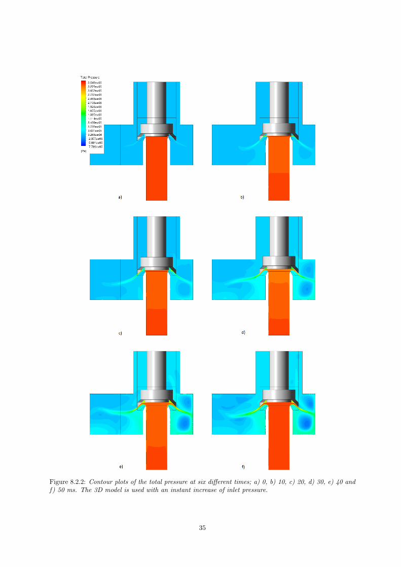
Figure 8.2.2: Contour plots of the total pressure at six different times; a) 0, b) 10, c) 20, d) 30, e) 40 andf) 50 ms. The 3D model is used with an instant increase of inlet pressure.

35

Figure 8.2.3: Vector plots of the velocity distribution at six different times; a) 0, b) 10, c) 20, d) 30, e) 40and f) 50 ms.

36

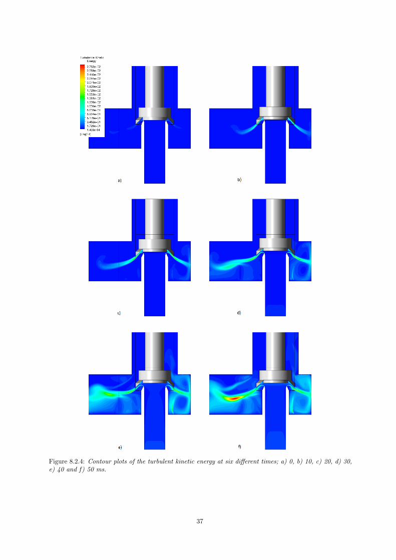
Figure 8.2.4: Contour plots of the turbulent kinetic energy at six different times; a) 0, b) 10, c) 20, d) 30,e) 40 and f) 50 ms.

37

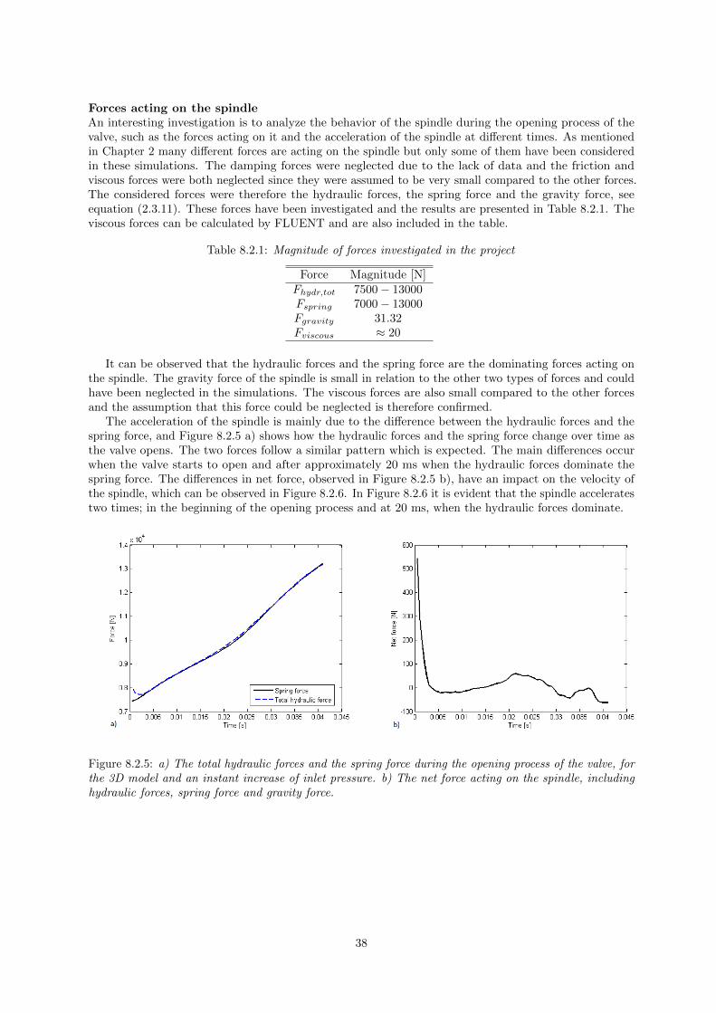
Forces acting on the spindleAn interesting investigation is to analyze the behavior of the spindle during the opening process of thevalve, such as the forces acting on it and the acceleration of the spindle at different times. As mentionedin Chapter 2 many different forces are acting on the spindle but only some of them have been consideredin these simulations. The damping forces were neglected due to the lack of data and the friction andviscous forces were both neglected since they were assumed to be very small compared to the other forces.The considered forces were therefore the hydraulic forces, the spring force and the gravity force, seeequation (2.3.11). These forces have been investigated and the results are presented in Table 8.2.1. Theviscous forces can be calculated by FLUENT and are also included in the table.

Table 8.2.1: Magnitude of forces investigated in the project

Force Magnitude [N]Fhydr,tot 7500− 13000Fspring 7000− 13000Fgravity 31.32Fviscous ≈ 20

It can be observed that the hydraulic forces and the spring force are the dominating forces acting onthe spindle. The gravity force of the spindle is small in relation to the other two types of forces and couldhave been neglected in the simulations. The viscous forces are also small compared to the other forcesand the assumption that this force could be neglected is therefore confirmed.

The acceleration of the spindle is mainly due to the difference between the hydraulic forces and thespring force, and Figure 8.2.5 a) shows how the hydraulic forces and the spring force change over time asthe valve opens. The two forces follow a similar pattern which is expected. The main differences occurwhen the valve starts to open and after approximately 20 ms when the hydraulic forces dominate thespring force. The differences in net force, observed in Figure 8.2.5 b), have an impact on the velocity ofthe spindle, which can be observed in Figure 8.2.6. In Figure 8.2.6 it is evident that the spindle acceleratestwo times; in the beginning of the opening process and at 20 ms, when the hydraulic forces dominate.

Figure 8.2.5: a) The total hydraulic forces and the spring force during the opening process of the valve, forthe 3D model and an instant increase of inlet pressure. b) The net force acting on the spindle, includinghydraulic forces, spring force and gravity force.

38

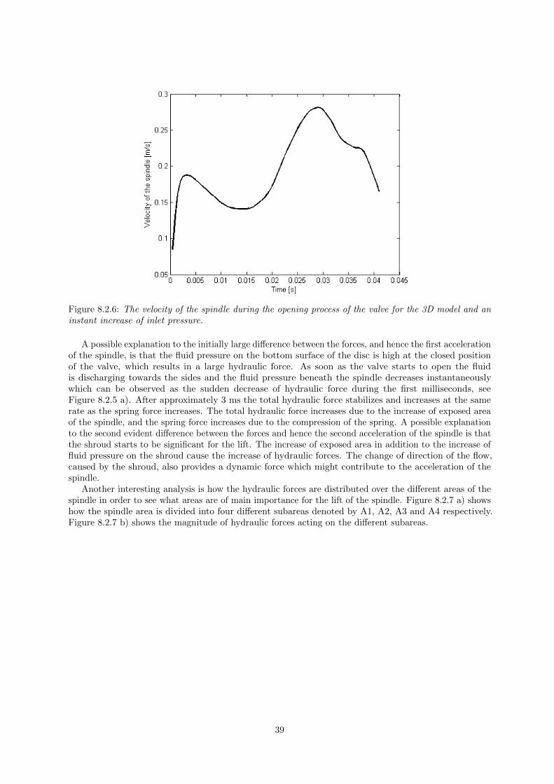
Figure 8.2.6: The velocity of the spindle during the opening process of the valve for the 3D model and aninstant increase of inlet pressure.

A possible explanation to the initially large difference between the forces, and hence the first accelerationof the spindle, is that the fluid pressure on the bottom surface of the disc is high at the closed positionof the valve, which results in a large hydraulic force. As soon as the valve starts to open the fluidis discharging towards the sides and the fluid pressure beneath the spindle decreases instantaneouslywhich can be observed as the sudden decrease of hydraulic force during the first milliseconds, seeFigure 8.2.5 a). After approximately 3 ms the total hydraulic force stabilizes and increases at the samerate as the spring force increases. The total hydraulic force increases due to the increase of exposed areaof the spindle, and the spring force increases due to the compression of the spring. A possible explanationto the second evident difference between the forces and hence the second acceleration of the spindle is thatthe shroud starts to be significant for the lift. The increase of exposed area in addition to the increase offluid pressure on the shroud cause the increase of hydraulic forces. The change of direction of the flow,caused by the shroud, also provides a dynamic force which might contribute to the acceleration of thespindle.

Another interesting analysis is how the hydraulic forces are distributed over the different areas of thespindle in order to see what areas are of main importance for the lift of the spindle. Figure 8.2.7 a) showshow the spindle area is divided into four different subareas denoted by A1, A2, A3 and A4 respectively.Figure 8.2.7 b) shows the magnitude of hydraulic forces acting on the different subareas.

39

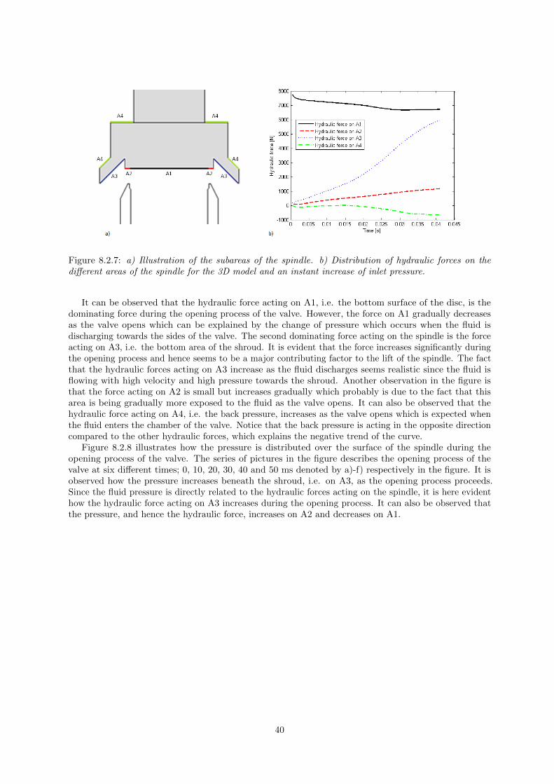
Figure 8.2.7: a) Illustration of the subareas of the spindle. b) Distribution of hydraulic forces on thedifferent areas of the spindle for the 3D model and an instant increase of inlet pressure.

It can be observed that the hydraulic force acting on A1, i.e. the bottom surface of the disc, is thedominating force during the opening process of the valve. However, the force on A1 gradually decreasesas the valve opens which can be explained by the change of pressure which occurs when the fluid isdischarging towards the sides of the valve. The second dominating force acting on the spindle is the forceacting on A3, i.e. the bottom area of the shroud. It is evident that the force increases significantly duringthe opening process and hence seems to be a major contributing factor to the lift of the spindle. The factthat the hydraulic forces acting on A3 increase as the fluid discharges seems realistic since the fluid isflowing with high velocity and high pressure towards the shroud. Another observation in the figure isthat the force acting on A2 is small but increases gradually which probably is due to the fact that thisarea is being gradually more exposed to the fluid as the valve opens. It can also be observed that thehydraulic force acting on A4, i.e. the back pressure, increases as the valve opens which is expected whenthe fluid enters the chamber of the valve. Notice that the back pressure is acting in the opposite directioncompared to the other hydraulic forces, which explains the negative trend of the curve.

Figure 8.2.8 illustrates how the pressure is distributed over the surface of the spindle during theopening process of the valve. The series of pictures in the figure describes the opening process of thevalve at six different times; 0, 10, 20, 30, 40 and 50 ms denoted by a)-f) respectively in the figure. It isobserved how the pressure increases beneath the shroud, i.e. on A3, as the opening process proceeds.Since the fluid pressure is directly related to the hydraulic forces acting on the spindle, it is here evidenthow the hydraulic force acting on A3 increases during the opening process. It can also be observed thatthe pressure, and hence the hydraulic force, increases on A2 and decreases on A1.

40

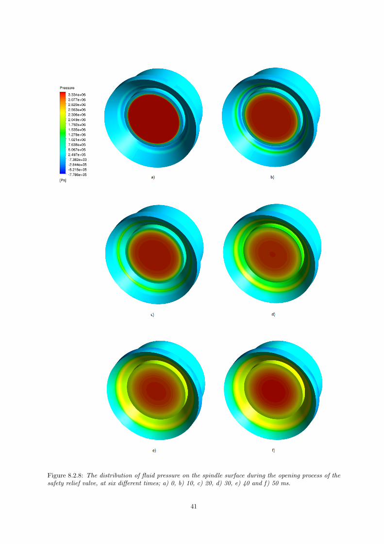
Figure 8.2.8: The distribution of fluid pressure on the spindle surface during the opening process of thesafety relief valve, at six different times; a) 0, b) 10, c) 20, d) 30, e) 40 and f) 50 ms.

41

8.2.2 2D model - Instant increase of inlet pressure

A simulation with an instant increase of inlet pressure to 34.1 bar(g) was also performed with the 2Dmodel. Figure 8.2.9 shows the opening profile of the valve, both for the 2D and the 3D models. Eventhough the total opening time for both models are nearly the same; 42.5 ms for the 2D model and 41 msfor the 3D model, the behavior of the opening process differs slightly between the two models.

Figure 8.2.9: Opening profile of the valve when the inlet pressure is instantly increased, both for the 2Dmodel and the 3D model.

The velocity of the spindle in the 2D and 3D simulations can be observed in Figure 8.2.10. In thisfigure the difference between the 2D and 3D models is even more distinguishable. During the first 30 msof the opening process the velocity of the spindle is lower with the 2D model than with the 3D model.But during the last milliseconds of the simulation the velocity of the spindle increases significantly for the2D model. These observations explain the differences seen in Figure 8.2.9 and also why the total openingtime between the two models do not differ much.

Figure 8.2.10: Velocity of the spindle during the opening process of the valve for an instant increase ofinlet pressure, both for the 2D model and the 3D model.

42

Figure 8.2.11 might give an explanation to why the 2D model of the valve behaves differently thanthe 3D model. The figure shows the hydraulic forces acting on the different parts of the spindle for the2D and the 3D simulation respectively. The hydraulic forces acting on A1 and A2 behave similarly inboth simulations. But the hydraulic force due to back pressure, denoted as the hydraulic force on A4, isalmost zero during the entire simulation of the opening process with the 2D model. This is a consequenceof using axisymmetry as a boundary in the model. The outlet of the valve model is open all the wayaround the valve since the 2D plane is rotated 360◦ around the symmetry axis. Since the outlet is largerin the model than in reality the back pressure does not build up as it should, which causes a difference inbehavior between the 2D and the 3D models.

Another major difference between the models can be observed in Figure 8.2.11. As mentioned earlier,the hydraulic force on A3 represents the hydraulic force acting on the bottom area of the shroud. Whenthe corresponding curves for the 2D and the 3D simulations are compared it is evident that the hydraulicforce acting on the shroud in the 2D model is lower than in the 3D model. This difference probablycontributes to the difference in behavior during the opening process observed earlier. Since the hydraulicforce is calculated differently in the two models it is expected that the results may differ. In the 3D modelthe pressure on the spindle is calculated in each cell and multiplied with the cell area whereas in the 2Dmodel the average pressure is calculated for each of the four subareas of the spindle and then multipliedwith the area for each subarea.

Figure 8.2.11: Comparison of the hydraulic forces acting on the different areas of the spindle during theopening process of the valve for the 2D and 3D model, for an instant increase of inlet pressure.

Figure 8.2.12 shows the contour plots of a) the total pressure and b) the turbulent kinetic energy,and c) a vector plot of the fluid velocity when the valve is fully open at 50 ms. It can be observed thatthe contour plot of turbulent kinetic energy in the 2D model differs significantly from the contour plotof turbulent kinetic energy in the 3D model, see Figure 8.2.4. The kinetic energy is larger beneath theshroud in the 2D model. This indicates that the turbulence is different in the 2D model compared to the3D model. Since the turbulence is affecting the fluid pressure, this results in different hydraulic forcesbetween the 2D and 3D models. In Figure 8.2.12 it can also be observed that there is almost no backpressure and that the fluid velocities are very low in the outlet since the outlet is large.

43

Figure 8.2.12: Contour plots of a) the total pressure and b) the turbulent kinetic energy, and c) a vectorplot of the velocity, when the valve is fully open at 50 ms for the 2D model and an instant increase of inletpressure.

44

8.2.3 Gradual increase of inlet pressure

In order to further investigate the features of the safety relief valve, a gradual increase of the inlet pressurewas performed where the inlet pressure increased linearly from 30.5 bar(g) until the valve was completelyopen. The linear equation (6.5.1) is an approximation of how the pressure was gradually increased duringexperiments.

In Figure 8.2.13 the static and dynamic pressure respectively, at the inlet of the valve, are presentedfor the 3D simulation when the inlet pressure is gradually increased. It is evident that the static pressureis gradually increased until the valve starts to open at 32.4 bar(g). At that moment the fluid starts todischarge out of the valve and the static pressure converts into dynamic pressure which is a functionof the fluid velocity. The static pressure rapidly decreases to approximately 29.6 bar(g) where it stayssomewhat constant which implies that the valve fulfills its purpose by keeping the pressure in the systemat an acceptable level.

Figure 8.2.13: a) Static pressure and b) dynamic pressure at the inlet of the valve during the openingprocess when the inlet pressure is gradually increased.

Figure 8.2.14 shows the lift of the spindle when the inlet pressure is gradually increased, both forthe 3D and 2D simulations. In the figure the experimental data are also included in order to validatethe results from the simulations with the reality. It can be observed that the experimental data followthree trends. The valve starts to open at 31 bar(g) and in the beginning of the opening process the valveopens slowly in relation to the increase of pressure. When the valve has lifted approximately 2 mm theopening process accelerates and the valve opens rapidly to an approximate lift of 7 mm. The remaininglift proceeds slowly until the maximum lift is reached. It can be observed that the 3D simulation followsthe two latter trends similarly. The simulation lacks the first gradual lifting process and opens at a higherpressure than the experimental data which probably is due to that the model is 5 % opened at the startingposition. The valve opens rapidly from 0.425 mm to 7.5 mm where a dip occurs. The final gradualincrease of the lift is similar to the experimental data and proceeds until the valve is completely opened.In the 2D simulation the valve opens slightly during the first part of the opening process similar to theexperimental data, but opens rapidly from 1 mm to 8.5 mm and thus lacks the final smooth opening. The2D simulation opens at an even higher pressure compared to the experimental data and the 3D simulation,which is probably due to the initial opening of 5 %. Another possible explanation to the late openingduring the 2D simulation might be due to the fact that the hydraulic forces acting on the bottom surfaceof the shroud are smaller than in the 3D simulation which cause a delayed opening process.

45

Figure 8.2.14: Comparison of the lift of the spindle when the inlet pressure is gradually increased for the2D model, the 3D model and experimental data.

The rapid opening which occurs in both the 2D and the 3D simulations is probably a result of the highacceleration which the spindle gets during the opening process. This can be observed in Figure 8.2.15which shows how the velocity of the spindle increases significantly as soon as the valve starts to open inthe 3D simulation. The initial time, t = 0, corresponds to when the inlet pressure was 30.5 bar(g) and theelapsed time is associated with the gradual increase of inlet pressure.

Figure 8.2.15: Velocity of the spindle during the opening process when the inlet pressure is graduallyincreased during the 3D simulation.

A possible explanation to the high acceleration of the spindle is that the spindle may include morestructures which are not considered in this project, which in that case means that the mass of the spindleis too small. Another source of error concerning the spindle might also be that some dimensions of the

46

spindle were not given in the drawing and they were therefore estimated for this project. This uncertaintyaffects the estimation of the volume of the spindle and hence its mass. An additional explanation tothe high acceleration of the spindle might be that damping forces are neglected in these simulations. Ifdamping would have been included, rapid accelerations would be slowed down and the opening process ofthe valve would be smoother. The high acceleration of the spindle might also be the reason why a dipoccurs at a lift of 7.5 mm in the 3D simulation. Due to the high acceleration of the spindle, it moves toorapidly upwards until the spring force becomes larger than the hydraulic force and makes it stop. Thespindle then has to wait for the inlet pressure to increase further in order to overcome the spring forceand the increase of back pressure which occurs during discharge. When this is accomplished the openingprocess can be completed.

One explanation to why the valve in the 2D simulation opens completely without the slower part inthe end of the opening process, seen in Figure 8.2.14, is probably due to the lack of back pressure which isa result of the outlet geometry for the axisymmetric case.

In Figure 8.2.14 it can also be observed that the valve is fully open at a lower pressure than 34.1 bar(g)for both the 2D and 3D simulations. The high acceleration of the spindle and thus the rapid opening ofthe valve is probably the cause to this behavior. Worth mentioning is that the experimental data alsoshow that the valve was fully open at a pressure lower than 34.1 bar(g).

Figure 8.2.16 shows how the lift of the spindle changes with time for the 3D simulation, 2D simulationand experimental data. As mentioned before, t = 0 corresponds to when the inlet pressure was 30.5 bar(g)and the elapsed time is associated with the increase of inlet pressure. The time it takes for the valve tobe fully opened counted from the start of the simulation was approximately 1.3 s for the 2D model and1.55 s for the 3D model. For the experiments the corresponding time was approximately 2.4 s. The largedifference in opening time between the models and the experimental data is probably due to that thelinear approximation of the increase in inlet pressure does not correctly represent the actual increase ofpressure used in the experiments, see Figure 8.2.17. In this figure it is evident that the inlet pressure inthe experiments are affected by the opening process of the valve which causes the nonlinear behavior at16 s. The difference between the experimental data and the approximated linear equation may explain whydifferences occur in Figure 8.2.16. This does not mean that the CFD models are incorrect, only that thegradual pressure increase proceeds differently in the CFD simulations compared to the experiments. Thedifference in opening time might also be due to the large acceleration of the spindle during the openingprocess.

Figure 8.2.16: Comparison of opening times of the valve when the inlet pressure is gradually increased forthe 2D model, the 3D model and experimental data.

47

Figure 8.2.17: Experimental gradual increase of inlet pressure and linear approximation of the gradualincrease used in this project.

The opening processes can be related to how the hydraulic forces are acting on the different subareason the spindle. The pictures in figure 8.2.18 show the distribution of hydraulic forces in the 3D and 2Dsimulation respectively, during the gradual increase of inlet pressure. By observing these pictures it is clearthat even though the hydraulic forces on the different subareas follow the same trends in both models, thehydraulic forces in the 2D model are delayed. This explains why the 2D model opens later than the 3Dmodel, which was observed in Figure 8.2.16, and at a higher pressure, which was observed in Figure 8.2.14.

Figure 8.2.18: Distribution of hydraulic forces acting on the different areas of the spindle during theopening process of the valve for a) the 3D model and b) the 2D model, when the inlet pressure was graduallyincreased.

When the data from the 3D simulation were analyzed further some interesting features were found,such as that the mass flow and the total hydraulic force follow a very similar pattern during the openingprocess of the valve, see Figure 8.2.19. This behavior is also similar to the hydraulic force acting on A3,which was observed in Figure 8.2.18 a). From these findings it is evident that the mass flow might havean impact on the total hydraulic force since they behave in a similar way.

48

Figure 8.2.19: a) Mass flow through the valve and b) total hydraulic force acting on the spindle during theopening process of the valve when the inlet pressure was gradually increased.

In order to implement the CFD results in RELAP5, a relation between the total hydraulic force andthe parameters available in RELAP5 is necessary. The fluid pressures and hence the hydraulic forcesacting on the surfaces of the spindle can partly be explained by the total pressure, consisting of a staticand a dynamic pressure, at the inlet and outlet of the valve. However, in this case when the geometryis complex, the inlet and outlet pressures are not enough to explain the total hydraulic force acting onthe spindle. The remaining part of the force might be possible to express with the mass flow throughthe valve. Since the mass flow is clearly related to the total hydraulic force, which was observed inFigure 8.2.19, it is possible that the mass flow which is flowing towards the shroud during dischargecontributes to the pressure beneath the shroud, creating the large hydraulic force acting on A3. Themass flow in the valve might therefore be an important variable related to the shape and the angle of theshroud when describing how the hydraulic forces are acting on the spindle.

Five equations, (8.2.1)-(8.2.5), describing the total hydraulic force acting on the spindle, are proposedwhere it is assumed that the force is a function of different pressures in the valve and the mass flowthrough the valve. In equation (8.2.1) the total hydraulic force depends on the inlet pressure and the massflow. The inlet pressure is divided into a static and a dynamic pressure, since RELAP5 does not use thetotal pressure in the calculations. In equation (8.2.2) an additional term, Pbackpressure, is added describingthat the total hydraulic force also depends on the back pressure in the valve. Both these equations includethe unknown constants α and β. Equation (8.2.2) and (8.2.3) are very similar; they both describe thetotal hydraulic force as a function of the pressure difference between inlet pressure and back pressure, andthe mass flow. The main difference between the equations is that the back pressure in equation (8.2.3)has its own constant, γ. In equation (8.2.4) and (8.2.5) the back pressure is replaced by an expression forthe static and dynamic pressure at the outlet of the valve. These two equations follow the same structureas equations (8.2.2) and (8.2.3), where the only difference between the equations is that a constant γ isincluded in the last equation.

Fh = α(Pstat,in +1

2ρU2

1 ) + βm (8.2.1)

Fh = α[(Pstat,in +1

2ρU2

1 )− Pbackpressure] + βm (8.2.2)

Fh = α(Pstat,in +1

2ρU2

1 ) + γPbackpressure + βm (8.2.3)

Fh = α[(Pstat,in +1

2ρU2

1 )− (Pstat,out +1

2ρU2

2 )] + βm (8.2.4)

Fh = α(Pstat,in +1

2ρU2

1 ) + γ(Pstat,out +1

2ρU2

2 ) + βm (8.2.5)

49

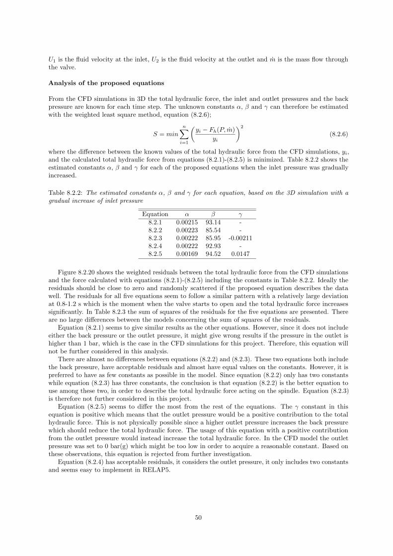
U1 is the fluid velocity at the inlet, U2 is the fluid velocity at the outlet and m is the mass flow throughthe valve.

Analysis of the proposed equations

From the CFD simulations in 3D the total hydraulic force, the inlet and outlet pressures and the backpressure are known for each time step. The unknown constants α, β and γ can therefore be estimatedwith the weighted least square method, equation (8.2.6);

S = min

n∑i=1

(yi − Fh(P, m)

yi

)2

(8.2.6)

where the difference between the known values of the total hydraulic force from the CFD simulations, yi,and the calculated total hydraulic force from equations (8.2.1)-(8.2.5) is minimized. Table 8.2.2 shows theestimated constants α, β and γ for each of the proposed equations when the inlet pressure was graduallyincreased.

Table 8.2.2: The estimated constants α, β and γ for each equation, based on the 3D simulation with agradual increase of inlet pressure

Equation α β γ8.2.1 0.00215 93.14 -8.2.2 0.00223 85.54 -8.2.3 0.00222 85.95 -0.002118.2.4 0.00222 92.93 -8.2.5 0.00169 94.52 0.0147

Figure 8.2.20 shows the weighted residuals between the total hydraulic force from the CFD simulationsand the force calculated with equations (8.2.1)-(8.2.5) including the constants in Table 8.2.2. Ideally theresiduals should be close to zero and randomly scattered if the proposed equation describes the datawell. The residuals for all five equations seem to follow a similar pattern with a relatively large deviationat 0.8-1.2 s which is the moment when the valve starts to open and the total hydraulic force increasessignificantly. In Table 8.2.3 the sum of squares of the residuals for the five equations are presented. Thereare no large differences between the models concerning the sum of squares of the residuals.

Equation (8.2.1) seems to give similar results as the other equations. However, since it does not includeeither the back pressure or the outlet pressure, it might give wrong results if the pressure in the outlet ishigher than 1 bar, which is the case in the CFD simulations for this project. Therefore, this equation willnot be further considered in this analysis.

There are almost no differences between equations (8.2.2) and (8.2.3). These two equations both includethe back pressure, have acceptable residuals and almost have equal values on the constants. However, it ispreferred to have as few constants as possible in the model. Since equation (8.2.2) only has two constantswhile equation (8.2.3) has three constants, the conclusion is that equation (8.2.2) is the better equation touse among these two, in order to describe the total hydraulic force acting on the spindle. Equation (8.2.3)is therefore not further considered in this project.

Equation (8.2.5) seems to differ the most from the rest of the equations. The γ constant in thisequation is positive which means that the outlet pressure would be a positive contribution to the totalhydraulic force. This is not physically possible since a higher outlet pressure increases the back pressurewhich should reduce the total hydraulic force. The usage of this equation with a positive contributionfrom the outlet pressure would instead increase the total hydraulic force. In the CFD model the outletpressure was set to 0 bar(g) which might be too low in order to acquire a reasonable constant. Based onthese observations, this equation is rejected from further investigation.

Equation (8.2.4) has acceptable residuals, it considers the outlet pressure, it only includes two constantsand seems easy to implement in RELAP5.

50

Figure 8.2.20: Weighted residuals between the total hydraulic force calculated from CFD simulations andwith the equations (8.2.1)-(8.2.5).

Table 8.2.3: The sum of squares of the residuals for the five equations (8.2.1)-(8.2.5)

Equation Weighted least square8.2.1 0.0438.2.2 0.0328.2.3 0.0328.2.4 0.0478.2.5 0.030

51

Equations (8.2.2) and (8.2.4) were chosen to be implemented in the servo valve model in RELAP5.Both equations seem to describe the CFD model relatively well, see Figure 8.2.21.

Figure 8.2.21: a) The total hydraulic force acting on the spindle with the 3D CFD model and with equation(8.2.2). b) The total hydraulic force with the 3D CFD model and with equation (8.2.4).

The constants α, β and γ were also estimated based on data acquired from the 3D simulation withan instant increase of inlet pressure, see Table 8.2.4. Since these values are similar to the constants inTable 8.2.2, which are based on a gradual increase of pressure, this indicates that the constants areindependent of the inlet boundary condition.

Table 8.2.4: The estimated constants α, β and γ for each equation, based on the 3D simulation with aninstant increase of inlet pressure

Equation α β γ8.2.1 0.00200 93.12 -8.2.2 0.00207 88.92 -8.2.3 0.00223 85.26 -0.003888.2.4 0.00205 93.12 -8.2.5 0.00200 93.12 0

Interpretation of α and βBy observing the purposed equations (8.2.2) and (8.2.4), it is evident that the first term has similaritieswith the primary equation describing hydraulic forces, F = PA. It can therefore be assumed that theconstant α corresponds to some kind of area. When analyzing the calculated values of α it was observedthat the values seem to correspond to the cross-sectional area of the inlet pipe of the valve in this project.More exactly, the values seem to correspond to the mean value of the pipe inlet area, since the inlet pipebecomes slightly wider closer to the spindle.

For the second term, which includes the constant β, it is more difficult to find an exact meaning.Probably the term can be related to the shroud, since the hydraulic force acting on A3 increases significantlyduring discharge. It is possible that the term is equal to 0 if the disc lacks a shroud. The exact meaningof the constant β is thus difficult to define. However, the unit of β is m/s which means that the constantcorresponds to some kind of velocity. The magnitude of β is approximately 93 m/s which is higher thanthe maximum fluid velocity through the safety relief valve. Probably the constant takes the geometry ofthe spindle into consideration which increases the value of β.

52

8.3 One-dimensional simulations of the safety relief valve

In this section the results from the RELAP5 simulations of the safety relief valve are presented. Firstly,the results from the motor valve model are presented and discussed. The currently used motor valvemodel is compared with the modified motor valve model where new input data are implemented. This isfollowed by the results from the servo valve model where amongst others the relations found from theCFD simulations are implemented.

8.3.1 Motor valve model

In the currently used motor valve model an opening time of 1 ms, an instant increase of inlet pressure andthe abrupt area change model are used. With these settings, the simulated valve generates higher forcesin the pipe systems than in reality. One of the aims in this project was therefore to try to improve thesimulations in order to reduce the unrealistic forces created in the systems.

Firstly, a new opening time was implemented in the model. When the valve was simulated in 3Din FLUENT with an instant increase of inlet pressure the opening time of the valve was 41 ms, whichis considered as more realistic than 1 ms. This opening time was used as input data in RELAP5 andthe abrupt area change model was still used. The pipes in the system were subdivided into 20 smallersegments with a length of 0.1 m each. For the abrupt area change model a constant value of the energyloss coefficient K was calculated from the CFD result and used as input. The value given is a measureof the energy loss in the valve when it is fully open and RELAP5 changes this value depending on theopening of the valve. The K value was calculated to 3.593 from equation (5.2.1) (K = ∆P/(ρU2/2))which resulted in a maximum mass flow of 63.7 kg/s through the valve which is similar to the CFD resultand the maximum capacity given in the original drawing.

Figure 8.3.1 shows the forces generated in the pipe right after the valve, from the currently usedmotor valve model with an opening time of 1 ms and the modified model with an opening time of 41 msrespectively. It can be observed that the forces are reduced by the implementation of the new openingtime. The forces in the pipe prior to the valve show a similar behavior. The two curves in Figure 8.3.1show a different behavior of the forces which apparently depends on the difference in opening time ofthe valve. The fluctuations in the currently used valve model are a result from Joukowski effects whichare due to that the valve opens too rapidly and generates limitations of the pressure drop. The modifiedvalve model generates an instantaneous high force in the beginning of the opening process but the forcesdecline as the valve continues to open.

Figure 8.3.1: Forces generated in the pipe after the valve for the currently used motor valve model and themodified motor valve model where the opening time of the valve is different.

53

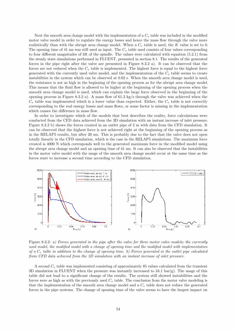
Next the smooth area change model with the implementation of a Cv table was included in the modifiedmotor valve model in order to regulate the energy losses and hence the mass flow through the valve morerealistically than with the abrupt area change model. When a Cv table is used, the K value is set to 0.The opening time of 41 ms was still used as input. The Cv table used consists of four values correspondingto four different magnitudes of lift of the spindle. The values were calculated with equation (5.2.1) fromthe steady state simulations performed in FLUENT, presented in section 8.1. The results of the generatedforces in the pipe right after the valve are presented in Figure 8.3.2 a). It can be observed that theforces are not reduced when the Cv table is implemented. The highest force is equal to the highest forcegenerated with the currently used valve model, and the implementation of the Cv table seems to createinstabilities in the system which can be observed at 0.02 s. When the smooth area change model is used,the resistance is not as high in the beginning of the opening process as for the abrupt area change model.This means that the fluid flow is allowed to be higher at the beginning of the opening process when thesmooth area change model is used, which can explain the large force observed in the beginning of theopening process in Figure 8.3.2 a). A mass flow of 61.3 kg/s through the valve was achieved when theCv table was implemented which is a lower value than expected. Either, the Cv table is not correctlycorresponding to the real energy losses and mass flows, or some factor is missing in the implementationwhich causes the difference in mass flow.

In order to investigate which of the models that best describes the reality, force calculations wereconducted from the CFD data achieved from the 3D simulation with an instant increase of inlet pressure.Figure 8.3.2 b) shows the forces created in an outlet pipe of 2 m with data from the CFD simulation. Itcan be observed that the highest force is not achieved right at the beginning of the opening process asin the RELAP5 results, but after 20 ms. This is probably due to the fact that the valve does not opentotally linearly in the CFD simulation, which is the case in the RELAP5 simulations. The maximum forcecreated is 4000 N which corresponds well to the generated maximum force in the modified model usingthe abrupt area change model and an opening time of 41 ms. It can also be observed that the instabilitiesin the motor valve model with the usage of the smooth area change model occur at the same time as theforces start to increase a second time according to the CFD simulation.

Figure 8.3.2: a) Forces generated in the pipe after the valve for three motor valve models; the currentlyused model, the modified model with a change of opening time and the modified model with implementationof a Cv table in addition to the change of opening time. b) Forces generated in the outlet pipe calculatedfrom CFD data achieved from the 3D simulation with an instant increase of inlet pressure.

A second Cv table was implemented consisting of approximately 85 values calculated from the transient3D simulation in FLUENT when the pressure was instantly increased to 34.1 bar(g). The usage of thistable did not lead to a significant change of the results. The system still showed instabilities and theforces were as high as with the previously used Cv table. The conclusion from the motor valve modeling isthat the implementation of the smooth area change model and a Cv table does not reduce the generatedforces in the pipe systems. The change of opening time of the valve seems to have the largest impact on

54

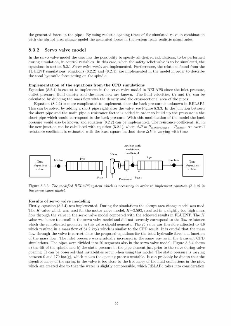
the generated forces in the pipes. By using realistic opening times of the simulated valve in combinationwith the abrupt area change model the generated forces in the system reach realistic magnitudes.

8.3.2 Servo valve model

In the servo valve model the user has the possibility to specify all desired calculations, to be performedduring simulation, in control variables. In this case, when the safety relief valve is to be simulated, theequations in section 5.2.1 Servo valve model are implemented. Furthermore, the relations found from theFLUENT simulations, equations (8.2.2) and (8.2.4), are implemented in the model in order to describethe total hydraulic force acting on the spindle.

Implementation of the equations from the CFD simulationsEquation (8.2.4) is easiest to implement in the servo valve model in RELAP5 since the inlet pressure,outlet pressure, fluid density and the mass flow are known. The fluid velocities, U1 and U2, can becalculated by dividing the mass flow with the density and the cross-sectional area of the pipes.

Equation (8.2.2) is more complicated to implement since the back pressure is unknown in RELAP5.This can be solved by adding a short pipe right after the valve, see Figure 8.3.3. In the junction betweenthe short pipe and the main pipe a resistance factor is added in order to build up the pressure in theshort pipe which would correspond to the back pressure. With this modification of the model the backpressure would also be known, and equation (8.2.2) can be implemented. The resistance coefficient, K, inthe new junction can be calculated with equation (5.2.1), where ∆P = Pbackpressure − Poutlet. An overallresistance coefficient is estimated with the least square method since ∆P is varying with time.

Figure 8.3.3: The modified RELAP5 system which is necessary in order to implement equation (8.2.2) inthe servo valve model.

Results of servo valve modelingFirstly, equation (8.2.4) was implemented. During the simulations the abrupt area change model was used.The K value which was used for the motor valve model, K=3.593, resulted in a slightly too high massflow through the valve in the servo valve model compared with the achieved results in FLUENT. The Kvalue was hence too small in the servo valve model and did not correctly correspond to the flow resistancewhich the complicated geometry in this valve should generate. The K value was therefore adjusted to 4.6which resulted in a mass flow of 64.2 kg/s which is similar to the CFD result. It is crucial that the massflow through the valve is correct since the proposed equations for the total hydraulic force is a functionof the mass flow. The inlet pressure was gradually increased in the same way as in the transient CFDsimulations. The pipes were divided into 20 segments also in the servo valve model. Figure 8.3.4 showsa) the lift of the spindle and b) the static pressure in the pipe element just prior to the valve during valveopening. It can be observed that instabilities occur when using this model. The static pressure is varyingbetween 0 and 170 bar(g), which makes the opening process unstable. It can probably be due to that theeigenfrequency of the spring in the valve is too close to the frequency of the fluid oscillations in the pipe,which are created due to that the water is slightly compressible, which RELAP5 takes into consideration.

55

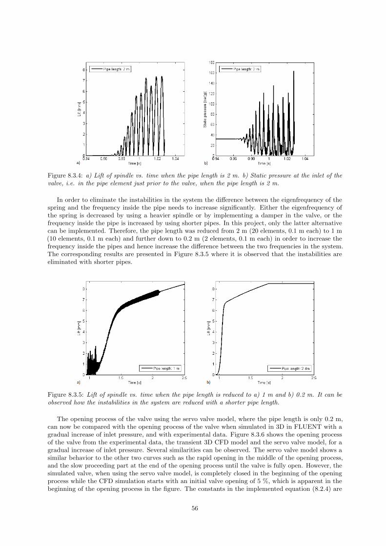
Figure 8.3.4: a) Lift of spindle vs. time when the pipe length is 2 m. b) Static pressure at the inlet of thevalve, i.e. in the pipe element just prior to the valve, when the pipe length is 2 m.

In order to eliminate the instabilities in the system the difference between the eigenfrequency of thespring and the frequency inside the pipe needs to increase significantly. Either the eigenfrequency ofthe spring is decreased by using a heavier spindle or by implementing a damper in the valve, or thefrequency inside the pipe is increased by using shorter pipes. In this project, only the latter alternativecan be implemented. Therefore, the pipe length was reduced from 2 m (20 elements, 0.1 m each) to 1 m(10 elements, 0.1 m each) and further down to 0.2 m (2 elements, 0.1 m each) in order to increase thefrequency inside the pipes and hence increase the difference between the two frequencies in the system.The corresponding results are presented in Figure 8.3.5 where it is observed that the instabilities areeliminated with shorter pipes.

Figure 8.3.5: Lift of spindle vs. time when the pipe length is reduced to a) 1 m and b) 0.2 m. It can beobserved how the instabilities in the system are reduced with a shorter pipe length.

The opening process of the valve using the servo valve model, where the pipe length is only 0.2 m,can now be compared with the opening process of the valve when simulated in 3D in FLUENT with agradual increase of inlet pressure, and with experimental data. Figure 8.3.6 shows the opening processof the valve from the experimental data, the transient 3D CFD model and the servo valve model, for agradual increase of inlet pressure. Several similarities can be observed. The servo valve model shows asimilar behavior to the other two curves such as the rapid opening in the middle of the opening process,and the slow proceeding part at the end of the opening process until the valve is fully open. However, thesimulated valve, when using the servo valve model, is completely closed in the beginning of the openingprocess while the CFD simulation starts with an initial valve opening of 5 %, which is apparent in thebeginning of the opening process in the figure. The constants in the implemented equation (8.2.4) are

56

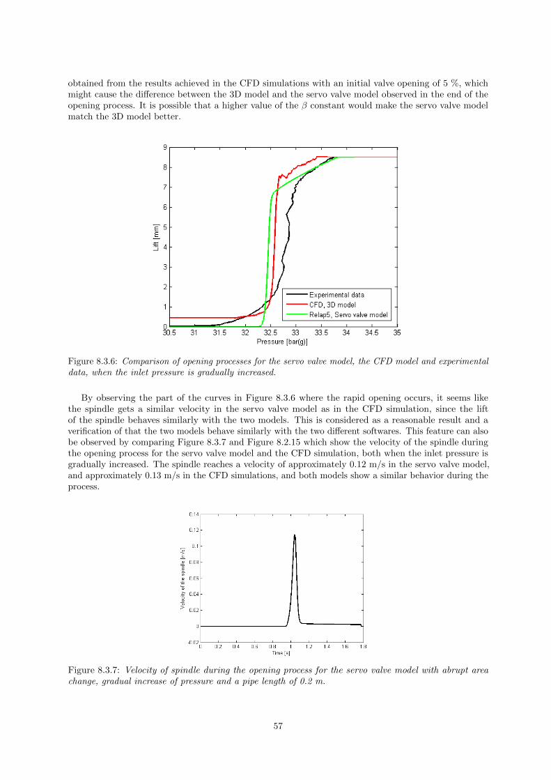
obtained from the results achieved in the CFD simulations with an initial valve opening of 5 %, whichmight cause the difference between the 3D model and the servo valve model observed in the end of theopening process. It is possible that a higher value of the β constant would make the servo valve modelmatch the 3D model better.

Figure 8.3.6: Comparison of opening processes for the servo valve model, the CFD model and experimentaldata, when the inlet pressure is gradually increased.

By observing the part of the curves in Figure 8.3.6 where the rapid opening occurs, it seems likethe spindle gets a similar velocity in the servo valve model as in the CFD simulation, since the liftof the spindle behaves similarly with the two models. This is considered as a reasonable result and averification of that the two models behave similarly with the two different softwares. This feature can alsobe observed by comparing Figure 8.3.7 and Figure 8.2.15 which show the velocity of the spindle duringthe opening process for the servo valve model and the CFD simulation, both when the inlet pressure isgradually increased. The spindle reaches a velocity of approximately 0.12 m/s in the servo valve model,and approximately 0.13 m/s in the CFD simulations, and both models show a similar behavior during theprocess.

Figure 8.3.7: Velocity of spindle during the opening process for the servo valve model with abrupt areachange, gradual increase of pressure and a pipe length of 0.2 m.

57

Another similarity between the servo valve model and the CFD simulation is how the static pressurechanges in the inlet of the valve as the valve opens, which can be observed by comparing Figures 8.3.8and 8.2.13 a). The two models behave very similarly which is yet another verification of that the twodifferent models seem to behave similarly in the two different softwares.

Figure 8.3.8: Static pressure at the inlet of the valve, i.e. in the pipe element just prior to the valve.

The forces generated in the pipe right after the valve were also investigated for the servo valve model,and the result is shown in Figure 8.3.9 a). The generated forces are very small, only with a magnitudeof approximately 180 N. This might not be a representative result since the pipes are very short, only0.2 m, and do not represent a system with long pipes. But since water is almost incompressible the forcesgenerated in a pipe with a length of 2 m would be increased with a factor of approximately 10, henceresulting in a force of 1800 N.

In order to compare the servo valve model with reality, the generated forces in the outlet pipe with alength of 0.2 m were also calculated from data achieved in the 3D CFD simulation with a gradual increaseof pressure. The result is shown in Figure 8.3.9 b). It can be observed that the same magnitude of force isgenerated both with the servo valve model and with the CFD simulation which is an indication that theservo valve model generates forces with a realistic magnitude. The main difference is that the main forceoccurs earlier in the RELAP5 simulation than in the CFD simulation which probably is due to the factthat the valve starts to open earlier in the RELAP5 simulation, which was observed in Figure 8.3.6.

Figure 8.3.9: a) Generated forces in the pipe right after the valve when the servo valve model with equation(8.2.4) and the abrupt area change model is implemented. b) Forces generated in the outlet pipe calculatedfrom CFD data achieved from the 3D simulation with a gradual increase of inlet pressure.

58

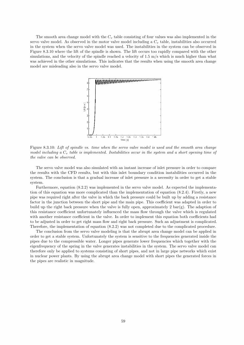
The smooth area change model with the Cv table consisting of four values was also implemented in theservo valve model. As observed in the motor valve model including a Cv table, instabilities also occurredin the system when the servo valve model was used. The instabilities in the system can be observed inFigure 8.3.10 where the lift of the spindle is shown. The lift occurs too rapidly compared with the othersimulations, and the velocity of the spindle reached a velocity of 1.5 m/s which is much higher than whatwas achieved in the other simulations. This indicates that the results when using the smooth area changemodel are misleading also in the servo valve model.

Figure 8.3.10: Lift of spindle vs. time when the servo valve model is used and the smooth area changemodel including a Cv table is implemented. Instabilities occur in the system and a short opening time ofthe valve can be observed.

The servo valve model was also simulated with an instant increase of inlet pressure in order to comparethe results with the CFD results, but with this inlet boundary condition instabilities occurred in thesystem. The conclusion is that a gradual increase of inlet pressure is a necessity in order to get a stablesystem.

Furthermore, equation (8.2.2) was implemented in the servo valve model. As expected the implementa-tion of this equation was more complicated than the implementation of equation (8.2.4). Firstly, a newpipe was required right after the valve in which the back pressure could be built up by adding a resistancefactor in the junction between the short pipe and the main pipe. This coefficient was adapted in order tobuild up the right back pressure when the valve is fully open, approximately 2 bar(g). The adaption ofthis resistance coefficient unfortunately influenced the mass flow through the valve which is regulatedwith another resistance coefficient in the valve. In order to implement this equation both coefficients hadto be adjusted in order to get right mass flow and right back pressure. Such an adjustment is complicated.Therefore, the implementation of equation (8.2.2) was not completed due to the complicated procedure.

The conclusion from the servo valve modeling is that the abrupt area change model can be applied inorder to get a stable system. Unfortunately the system is sensitive to the frequencies generated inside thepipes due to the compressible water. Longer pipes generate lower frequencies which together with theeigenfrequency of the spring in the valve generates instabilities in the system. The servo valve model cantherefore only be applied to systems consisting of short pipes, and not in large pipe networks which existin nuclear power plants. By using the abrupt area change model with short pipes the generated forces inthe pipes are realistic in magnitude.

59

9 Overall discussion

The safety relief valve in this project was simulated in both 3D and 2D. Since the computational time forthe 2D simulation is only a fractional part of the computational time for the 3D simulation, it is preferableto use the 2D model if possible. Both models result in similar opening times when an instant increase ofpressure was used as inlet boundary condition. Also, the order of magnitude of the hydraulic forces actingon the spindle are similar with some differences. The 2D model might therefore be correct enough to beused for some simpler applications such as calculation of the opening time of the valve. However, it isimportant to be aware of the differences in accuracy between the two models. In the 2D simulations withan instant increase of inlet pressure, the spindle moved more slowly during the first half of the openingprocess and faster at the end. The axisymmetric boundary condition used in the 2D model probablycontributes to the difference in opening behavior. The turbulence is different in the 2D model which alsoaffects the hydraulic forces acting on the spindle, causing the observed differences between the models.The 3D simulation where the inlet pressure was gradually increased showed a more realistic behavior ofthe opening process than the 2D simulation, from which one can conclude that the 3D simulation is morerealistic. In this project the results from the CFD simulations were used in order to find equations todescribe the total hydraulic forces acting on the spindle. In that case the results from the 2D simulationswere not satisfactory enough and the results from the 3D simulations were therefore used.

Since no CAD drawing was available, the geometry of the valve was created in ANSA. The geometrywas verified by calculating the forces acting on the spindle at different magnitudes of lift during steadystate simulations, and comparing the results with experimental data. This investigation concluded thatthe geometry and the force calculations seem to be consistent with reality. However, a CAD drawingwould probably have given even more correct results. Since all dimensions were not given in the availabledrawing, the created ANSA geometry is a source of error. It has been observed that small deviationsin dimensions of the inlet pipe or of the spindle can result in apparent differences in hydraulic forces.However, the meshing procedure with the aim to achieve a structured mesh had been more difficult witha CAD drawing, since some structures in the valve are rounded in reality.

One source of error with the CFD simulations in this project is that the valve cannot be completelyclosed at the start of the simulations, since a dynamic mesh method is needed in order to change themesh as the valve opens. In this project the dynamic layering method was used which requires at leastone layer of cells as starting condition. Another source of error in the CFD simulations is that it wasdifficult to decrease the y+ value around the spindle, since it had to be performed manually in ANSA.ANSYS FLUENT has a function where the mesh with high y+ values is refined, but this could not beused in this model without affecting the layer from which the mesh would be built up from.

The modified motor valve model with a realistic opening time of 41 ms generated lower forces in thepipe system than the currently used motor valve model with an opening time of 1 ms. However, the actualopening time is different for different valves and the opening time found in this project cannot be used forall cases. In order to make this type of modification in a motor valve model, the actual opening time forthe investigated valve must be acquired, for example from experiments or with a 2D CFD simulation.A 2D simulation will probably give an opening time which is accurate enough. But even though the2D simulations have short computational times, it still takes time to construct the actual model. Usingexperimental data, if available, would probably be the most efficient way to modify the model. However,the currently used motor valve model, with an opening time of 1 ms, might in some cases be good enoughand less time consuming.

Two of the five proposed equations describing the total hydraulic force acting on the spindle wereimplemented in the servo valve model in RELAP5. One of them, equation (8.2.4), showed similar openingbehavior and forces on the pipe system as the 3D CFD model. The other one, equation (8.2.2), wasdifficult to implement and did not open correctly. Both the CFD simulation in 3D and the servo valvemodel with equation (8.2.4) and with abrupt area change, open faster than the safety relief valve does inreality. These models do therefore not underestimate the forces acting on the pipe system which is in linewith the conservative requirements within nuclear engineering. However, the servo valve model cannotreplace the currently used motor valve model in all cases. With the settings in this project the servo valvemodel only works with short pipes. Usually large pipe systems are analyzed within nuclear engineering. Ifa damper is included in the model and/or the weight of the spindle is higher, this servo valve model mightwork with longer pipes. Furthermore, the servo valve model does not work when an instant increase of

60

inlet pressure is used as a boundary condition. This is another disadvantage for this servo valve model.It was observed that the implementation of the smooth area change model with a Cv table caused

instabilities in both the motor valve simulations and in the servo valve simulations. This was a disappointingresult, since the smooth area change model was expected to give more correct mass flows and hence lowerforces in the systems.

9.1 Conclusions

• The steady state simulations in CFD at different magnitudes of lift of the spindle showed that thecreated 3D geometry of the valve and the force calculations seem to be consistent with reality.

• The hydraulic forces and the spring force are the dominating forces contributing to the movement ofthe spindle.

• The CFD simulations in 2D and 3D show similarities, such as the opening time of the valve andthe order of magnitude of hydraulic forces, when the inlet pressure is instantly increased. However,some differences are evident between the models, such as the built up back pressure and the openingprocess during gradual increase of inlet pressure.

• The modified motor valve model with an opening time of 41 ms generates lower forces in the pipesystem than the currently used motor valve model.

• The total hydraulic force acting on the spindle can be described as a function of the inlet pressure,the outlet pressure and the mass flow.

• With present settings the servo valve model only works with short pipes and a gradual increase ininlet pressure as boundary condition. If the pipes are longer or if the inlet pressure is increasedinstantaneously instabilities occur in the system.

• The smooth area change model including a Cv table causes instabilities both in the motor valvemodel and in the servo valve model, which means that the abrupt area change model needs to beapplied in order to get a stable system.

• The 2D and 3D CFD models, and the servo valve model in RELAP5 open faster than the safetyrelief valve does in reality. This makes the models conservative which is a requirement within nuclearengineering.

9.2 Future studies

In future studies it would be interesting to find a method for simulating a safety relief valve in CFD froma completely closed position. Or at least make the initial opening smaller than 5 % and try to includemore layers beneath the spindle in order to be able to use the y+ adaption tool in ANSYS FLUENTwithout affecting the dynamic layering.

It would also be interesting to investigate if equation (8.2.4) for estimating the total hydraulic forceacting on the spindle also works for simulations of other safety relief valves and not only for the valveinvestigated in this project. The constant α is probably related to the cross-sectional area of the inlet ofthe valve, but how the β constant is exactly related to the valve is difficult to define.

It would be interesting to investigate why the servo valve model is unstable when the inlet pressure isincreased instantaneously. It would also be interesting to investigate why instabilities occur when thesmooth area change model with a Cv table is used.

61

References[1] Spirax Sarco. The steam and condensate loop book - An Engineer’s Best Practice Guide For Saving

Energy. 2011. isbn: 978-0-9550691-5-4.[2] Welty et al. Fundamentals of momentum, heat, and mass transfer. John Wiley and Sons, Inc., 2008.

isbn: 978-0470128688.[3] Connie J. Wells. Practice makes perfect - Physics. McGraw-Hill, USA, 2011. isbn: 9780071746960.[4] Avtar Singh. “An analytical study of the dynamics and stability of a spring loaded safety valve”. In:

Nuclear Engineering and Design 72 (1982), pp. 197–204.[5] ANSA. BETA CAE Systems USA, Inc., 2011. url: www.beta-cae.gr/ansa.htm,2012-04-12.[6] Bengt Andersson et al. Computational Fluid Dynamics for engineers. Gothenburg, Sweden, 2011.[7] Xue Guan Song et al. 2-D Dynamic Analysis of a Pressure Relief Valve by CFD. Proceedings of

the 9th WSEAS Int. Conference on Applied Computer and Applied Computational Science. isbn:978-960-474-173-1.

[8] Lin Wang Xue Guan Song and Young Chul Park. “Transient Analysis of a Spring-Loaded PressureSafety Valve Using Computational Fluid Dynamics (CFD)”. In: Journal of Pressure Vessel Technology132 (2010), pp. 054501–1 –054501–5.

[9] J. Francis and P. L. Betts. “Modelling incompressible flow in a pressure relief valve”. In: Proceedingsof the Instutution of Mechanical Engineers 211 (1997), pp. 83–93.

[10] ANSYS FLUENT 13. Theory guide. ANSYS Inc., 2010.[11] RELAP5/mod3.3 code manual. Volume I. Information systems laboratories, Inc., Rockville, Maryland,

Idaho Falls, Idaho, 2003.[12] RELAP5/mod3.3 code manual. Volume II. Information systems laboratories, Inc., Rockville, Mary-

land, Idaho Falls, Idaho, 2003.[13] Anders Bystrom. Oral reference. Ringhals NPP, 2012-04-10.

62

A Appendix - UDF

A.1 UDF for CFD simulation in 3D

#include "udf.h"

#include "mem.h"

/*global variables*/

static real k = 722150.0; /*spring constant*/

static real gravity = -9.81; /*gravity constant*/

static real x_max=0.0085; /*the maximum lift is 8.5 mm*/

static real f0=7126.0; /*initial spring force */

static real mass=3.1928; /*spindle mass*/

real total_force=0.0;

real pressure_force=0.0; /*the total hydraulic force over the entire spindle*/

real pressure_force1=0.0; /*hydraulic force beneath the disc, in contact with inlet*/

real pressure_force2=0.0; /*hydraulic force beneath the disc outside the seat*/

real pressure_force3=0.0; /*hydraulic force beneath the shroud*/

real pressure_force4=0.0; /*hydraulic force above the spindle */

real spring_force=0.0;

real x= 0.000425; /*simulation starts with an opening of 0.425 mm*/

real velocity1=0.0;

real velocity2=0.0;

real massflow=0.0;

real total_area1=0.0;

real total_area2=0.0;

real total_area3=0.0;

real mass_flow1=0.0;

real mass_flow2=0.0;

real mass_flow3=0.0;

real timestep=0.0;

real dx=0.008075;

real velocity =0.0;

real total_time=0.0;

real time_step=0.0;

real pressure=0.0;

real inlet_pressure=0.0;

/***********************************************************************************/

DEFINE_ADJUST(force_calculation,domain)

{

/* This function calculates the hydraulic forces acting on the spindle*/

int surface_thread_id1=26;

int surface_thread_id2=30;

int surface_thread_id3=31;

int surface_thread_id4=32;

pressure_force1=0.0;

pressure_force2=0.0;

pressure_force3=0.0;

pressure_force4=0.0;

#if !RP_HOST

Thread *thread1; /*structure data type that stores data that is common to the

group of cells or faces that it represents*/

Thread *thread2;

63

Thread *thread3;

Thread *thread4;

face_t face; /* an integer data type that indentifies

a particular face within a face thread*/

real area[ND_ND];

/*get the thread pointer for which this motion is defined*/

thread1 = Lookup_Thread(domain,surface_thread_id1);

thread2 = Lookup_Thread(domain,surface_thread_id2);

thread3 = Lookup_Thread(domain,surface_thread_id3);

thread4 = Lookup_Thread(domain,surface_thread_id4);

/*compute pressure forces on body by looping through all faces*/

begin_f_loop(face,thread1)

if (PRINCIPAL_FACE_P(face,thread1)) /* test if the face is the principle face*/

{

F_AREA(area,face,thread1);

pressure_force1+=area[2]*F_P(face,thread1);

}

end_f_loop(face,thread1)

begin_f_loop(face,thread2)

if (PRINCIPAL_FACE_P(face,thread2))

{

F_AREA(area,face,thread2);

pressure_force2+=area[2]*F_P(face,thread2);

}

end_f_loop(face,thread2)

begin_f_loop(face,thread3)

if (PRINCIPAL_FACE_P(face,thread3))

{

F_AREA(area,face,thread3);

pressure_force3+=area[2]*F_P(face,thread3);

}

end_f_loop(face,thread)

begin_f_loop(face,thread4)

if (PRINCIPAL_FACE_P(face,thread4))

{

F_AREA(area,face,thread4);

pressure_force4+=area[2]*F_P(face,thread4);

}

end_f_loop(face,thread4)

pressure_force=pressure_force1+pressure_force2+pressure_force3+pressure_force4;

#endif

#if RP_NODE

/*the value from all nodes are summed*/

pressure_force = PRF_GRSUM1(pressure_force);

pressure_force1 = PRF_GRSUM1(pressure_force1);

pressure_force2 = PRF_GRSUM1(pressure_force2);

pressure_force3 = PRF_GRSUM1(pressure_force3);

pressure_force4 = PRF_GRSUM1(pressure_force4);

#endif

64

/*the data from the nodes is sent to the host*/

node_to_host_real_5(pressure_force,pressure_force1,

pressure_force2, pressure_force3, pressure_force4);

/********************************************************************************/

DEFINE_ADJUST(velocity_calculation,domain)

{

int surface_thread_id1=5;

int surface_thread_id2=34;

int surface_thread_id3=13;

total_area1=0.0;

total_area2=0.0;

total_area3=0.0;

mass_flow1=0.0;

mass_flow2=0.0;

mass_flow3=0.0;

#if !RP_HOST

Thread *thread1;

Thread *thread2;

Thread *thread3;

face_t face;

real area[ND_ND];

thread1 = Lookup_Thread(domain,surface_thread_id1);

thread2 = Lookup_Thread(domain,surface_thread_id2);

thread3 = Lookup_Thread(domain,surface_thread_id3);

begin_f_loop(face,thread1)

if (PRINCIPAL_FACE_P(face,thread1))

{

F_AREA(area,face,thread1);

total_area1 += NV_MAG(area);

mass_flow1+=F_FLUX(face,thread1);

}

end_f_loop(face,thread1)

begin_f_loop(face,thread2)

if (PRINCIPAL_FACE_P(face,thread2))

{

F_AREA(area,face,thread2);

total_area2 += NV_MAG(area);

mass_flow2+=F_FLUX(face,thread2);

}

end_f_loop(face,thread2)

begin_f_loop(face,thread3)

if (PRINCIPAL_FACE_P(face,thread3))

{

F_AREA(area,face,thread3);

total_area3 += NV_MAG(area);

mass_flow3+=F_FLUX(face,thread3);

65

}

end_f_loop(face,thread3)

#endif

#if RP_NODE

mass_flow1 = PRF_GRSUM1(mass_flow1);

mass_flow2 = PRF_GRSUM1(mass_flow2);

mass_flow3 = PRF_GRSUM1(mass_flow3);

total_area1 =PRF_GRSUM1(total_area1);

total_area2 =PRF_GRSUM1(total_area2);

total_area3 =PRF_GRSUM1(total_area3);

#endif

massflow=mass_flow1;

node_to_host_real_1(massflow);

}

/*******************************************************************************/

DEFINE_CG_MOTION(spindle, dt, vel, omega, time, dtime)

{

/*reset velocities*/

NV_S(vel, =, 0.0);

NV_S(omega,=, 0.0); /*no angular motion*/

/*set y-component of velocity*/

vel[2] = velocity;

/*variable needed in execute_at_end*/

timestep=dtime;

}

/********************************************************************************/

DEFINE_EXECUTE_AT_END(Velocity)

{

/*Calculation of velocity*/

real dv=0;

real gravity_force=0.0;

spring_force=0.0;

/* calculate the total force acting on the spindle*/

gravity_force = mass*gravity;

/*calculate the spring force*/

spring_force = -k*x - f0;

/*calculate the total hydraulic force since mirror symmetry is used*/

pressure_force=pressure_force*2;

total_force=pressure_force + gravity_force + spring_force;

dv = timestep * total_force/mass;

velocity+=dv;

66

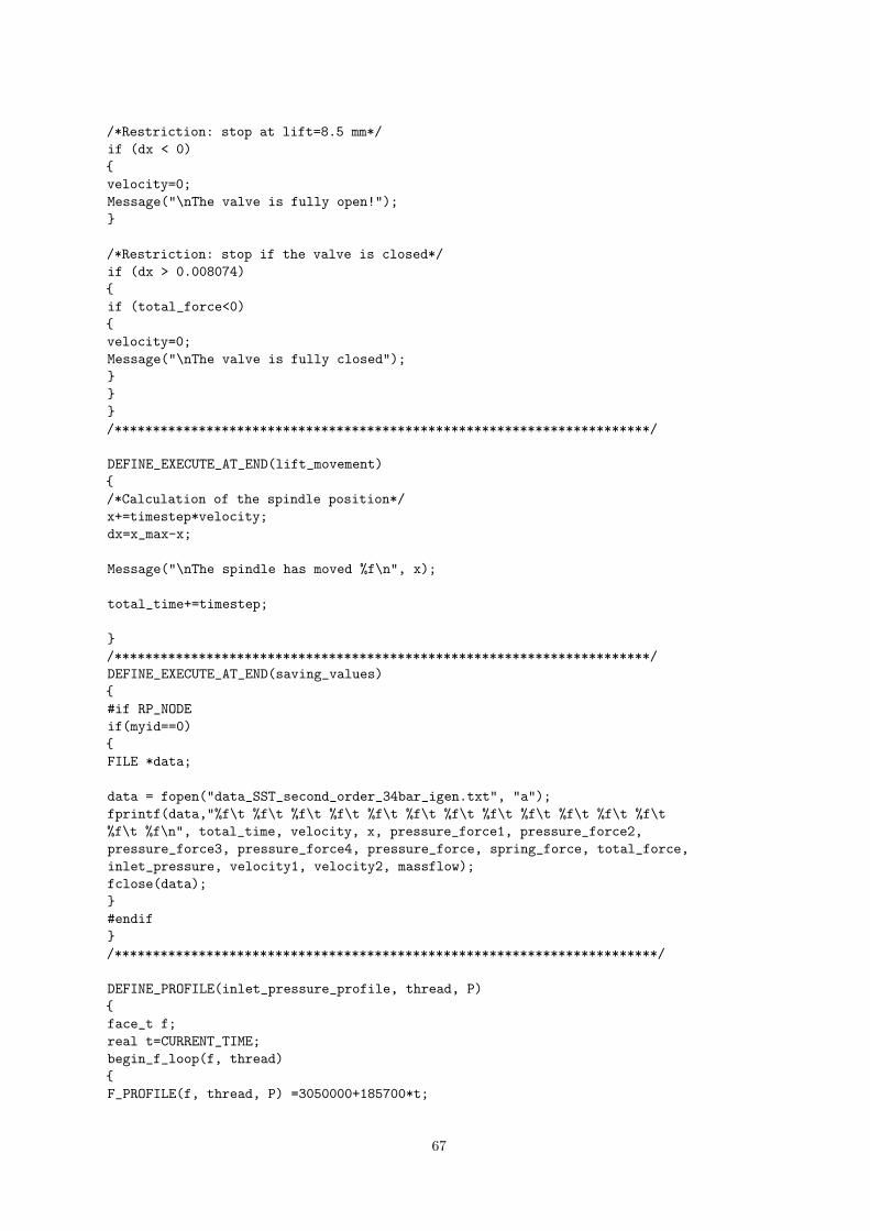
/*Restriction: stop at lift=8.5 mm*/

if (dx < 0)

{

velocity=0;

Message("\nThe valve is fully open!");

}

/*Restriction: stop if the valve is closed*/

if (dx > 0.008074)

{

if (total_force<0)

{

velocity=0;

Message("\nThe valve is fully closed");

}

}

}

/**********************************************************************/

DEFINE_EXECUTE_AT_END(lift_movement)

{

/*Calculation of the spindle position*/

x+=timestep*velocity;

dx=x_max-x;

Message("\nThe spindle has moved %f\n", x);

total_time+=timestep;

}

/**********************************************************************/

DEFINE_EXECUTE_AT_END(saving_values)

{

#if RP_NODE

if(myid==0)

{

FILE *data;

data = fopen("data_SST_second_order_34bar_igen.txt", "a");

fprintf(data,"%f\t %f\t %f\t %f\t %f\t %f\t %f\t %f\t %f\t %f\t %f\t %f\t

%f\t %f\n", total_time, velocity, x, pressure_force1, pressure_force2,

pressure_force3, pressure_force4, pressure_force, spring_force, total_force,

inlet_pressure, velocity1, velocity2, massflow);

fclose(data);

}

#endif

}

/***********************************************************************/

DEFINE_PROFILE(inlet_pressure_profile, thread, P)

{

face_t f;

real t=CURRENT_TIME;

begin_f_loop(f, thread)

{

F_PROFILE(f, thread, P) =3050000+185700*t;

67

}

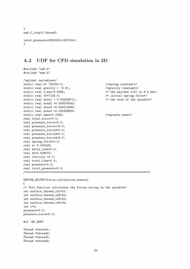
end_f_loop(f,thread)

inlet_pressure=3050000+185700*t;

}

A.2 UDF for CFD simulation in 2D

#include "udf.h"

#include "mem.h"

/*global variables*/

static real k= 722150.0; /*spring constant*/

static real gravity = -9.81; /*gravity constant*/

static real x_max=0.0085; /* the maximum lift is 8.5 mm*/

static real f0=7126.0; /* initial spring force*/

static real area1 = 0.002298711; /* the area of the spindle*/

static real area2 =0.000576042;

static real area3 =0.004213464;

static real area4 =0.005308694;

static real mass=3.1928; /*spindle mass*/

real total_force=0.0;

real pressure_force=0.0;

real pressure_force1=0.0;

real pressure_force2=0.0;

real pressure_force3=0.0;

real pressure_force4=0.0;

real spring_force=0.0;

real x= 0.000425;

real delta_time=0.0;

real dx=0.008075;

real velocity =0.0;

real total_time=0.0;

real pressure=0.0;

real inlet_pressure=0.0;

/**************************************************************************/

DEFINE_ADJUST(force_calculation,domain)

{

/* This function calculates the forces acting on the spindle*/

int surface_thread_id1=21;

int surface_thread_id2=22;

int surface_thread_id3=23;

int surface_thread_id4=24;

int i=0;

pressure=0.0;

pressure_force=0.0;

#if !RP_HOST

Thread *thread1;

Thread *thread2;

Thread *thread3;

Thread *thread4;

68

face_t face;

/*get the thread pointer for which this motion is defined*/

thread1 = Lookup_Thread(domain,surface_thread_id1);

thread2 = Lookup_Thread(domain,surface_thread_id2);

thread3 = Lookup_Thread(domain,surface_thread_id3);

thread4 = Lookup_Thread(domain,surface_thread_id4);

/*compute pressure forces on body by looping through all faces*/

begin_f_loop(face,thread1)

if (PRINCIPAL_FACE_P(face,thread1))

{

pressure+=F_P(face,thread1);

i+=1;

}

end_f_loop(face,thread)

if (i>0)

pressure_force1 =pressure/77 * area1;

if (i==0)

pressure_force1=0;

/*------------------------------------------*/

i=0;

pressure=0.0;

begin_f_loop(face,thread2)

if (PRINCIPAL_FACE_P(face,thread2))

{

pressure+=F_P(face,thread2);

i+=1;

}

end_f_loop(face,thread)

if (i>0)

pressure_force2 =pressure/22 * area2;

if (i==0)

pressure_force2=0;

/*---------------------------------------------*/

i=0;

pressure=0.0;

begin_f_loop(face,thread3)

if (PRINCIPAL_FACE_P(face,thread3)) /* test if the face is the principle face*/

{

pressure+=F_P(face,thread3);

i+=1;

}

end_f_loop(face,thread)

if (i>0)

pressure_force3 =pressure/43 * area3;

if (i==0)

pressure_force3=0;

/*---------------------------------------------------*/

69

i=0;

pressure=0.0;

begin_f_loop(face,thread4)

if (PRINCIPAL_FACE_P(face,thread4)) /* test if the face is the principle face*/

{

pressure+=F_P(face,thread4);

i+=1;

}

end_f_loop(face,thread)

if (i>0)

pressure_force4 =pressure/17 * area4;

if (i==0)

pressure_force4=0;

pressure_force=pressure_force1+pressure_force2+pressure_force3-pressure_force4;

#endif

#if RP_NODE

/*the value from all nodes are summed*/

pressure_force = PRF_GRSUM1(pressure_force);

pressure_force1 = PRF_GRSUM1(pressure_force1);

pressure_force2 = PRF_GRSUM1(pressure_force2);

pressure_force3 = PRF_GRSUM1(pressure_force3);

pressure_force4 = PRF_GRSUM1(pressure_force4);

#endif

/*the data from the nodes is sent to the host*/

node_to_host_real_5(pressure_force, pressure_force1, pressure_force2,

pressure_force3, pressure_force4);

}

/******************************************************************/

DEFINE_CG_MOTION(spindle, dt, vel, omega, time, dtime)

{

/*reset velocities*/

NV_S(vel, =, 0.0);

NV_S(omega,=, 0.0); /*no angular motion*/

/*set y-component of velocity*/

vel[0] = velocity;

/*variables needed in execute_at_end*/

delta_time=dtime;

}

/*****************************************************************/

DEFINE_EXECUTE_AT_END(lift_movement)

{

/*Calculation of the spindle position*/

x+=delta_time*velocity;

dx=x_max-x;

Message("\nThe spindle has moved %f\n", x);

total_time+=delta_time;

}

/*****************************************************************/

70

DEFINE_EXECUTE_AT_END(Velocity)

{

/*Calculation of velocity*/

/*Compute change in velocity, i.e., dv = F ’ dt/mass*/

real dv=0;

real gravity_force=0.0;

spring_force=0.0;

/* calculate the total force acting on the spindle*/

gravity_force = mass*gravity;

/*calculate the spring force*/

spring_force = -k*x -f0;

/*calculate total force*/

total_force = pressure_force + gravity_force +spring_force;

dv = delta_time * total_force/mass;

velocity+=dv;

/*Restriction: stop at lift=8.5 mm*/

if (dx < 0)

{

velocity=0;

Message("\nThe valve is fully open!");

}

if (dx > 0.008074)

{

if(total_force<0)

{

velocity=0;

Message("\nThe valve is fully closed");

}

}

}

/*******************************************************************/

DEFINE_EXECUTE_AT_END(saving_values)

{

#if RP_NODE

if(myid==0)

{

FILE *data;

data = fopen("data_2D_34_1bar_bra_massa.txt", "a");

fprintf(data,"%f\t %f\t %f\t %f\t %f\t %f\t %f\t %f\t

%f\t %f\t %f\n", total_time, velocity, x, pressure_force1,

pressure_force2, pressure_force3, pressure_force4, pressure_force,

spring_force, total_force, inlet_pressure);

fclose(data);

}

#endif

}

/*********************************************************************/

71

DEFINE_PROFILE(inlet_pressure_profile, thread, P)

{

face_t f;

real t=CURRENT_TIME;

begin_f_loop(f, thread)

{

F_PROFILE(f, thread, P) =3050000+185700*t;

}

end_f_loop(f,thread)

inlet_pressure=3050000+185700*t;

}

72

B Appendix - Motor valve modelIn this appendix the code for the currently used motor valve model, the modified motor valve model withabrupt area change and the modified model with smooth area change are presented. Since the code for thetime-dependent volumes, pipes etc. is the same for all three motor valve models it will only be describedonce.

B.1 Currently used motor valve model

*title standard ventil

=test.i

*==================================================================

* Problem type and option (card 100)

*==================================================================

0000100 new transnt *a new transient problem

*==================================================================

* Input check or run (card 101)

*==================================================================

0000101 run *the problem is executed if no errors are detected

*==================================================================

* Units selection (card 102)

*==================================================================

*input unit, output unit

0000102 si si * SI units

*==================================================================

* Timestep cards (201-299)

*==================================================================

* end min max ctrl minr-edt/plt majr-edt/plt rst-freq

0000201 100.0 1.0e-10 1.000e-002 7 100 1000000 1000000

0000202 105.0 1.0e-10 1.000e-005 7 13 1000000 1000000

*==================================================================

* Trip cards, variable trips (401-599)

*==================================================================

401 time 0 gt null 0 101.0 n * true if t>=101.0 s

402 time 0 ge null 0 200.0 n * true if t>=200.0 s

*==================================================================

* Control variable numbers

*==================================================================

20500000 9999

*==================================================================

* time-dependent volume component

*==================================================================

1000000 Tank1 tmdpvol

* Geometry card: area, length, volume, az-angle, inc-angle, elevation change

1000101 5.0 10.0000 0.0 0.0 0.0 0.0

* Geometry card: wall roughness, hydraulic diameter, volume_flags

1000102 0.000045 0.0 0

* Data control word card: ebt-flag trip alpha idnum

1000200 103 0 time 0

* Data card: time pressure temperature

1000201 0.0 3.51e+6 298.000

*==================================================================

* single junction 101

*==================================================================

1010000 junction sngljun

73

* Geometry card: from, to, area, forward flow energy loss,

*reverse flow energy loss, control flags: jefvcahs

1010101 100000000 102010001 0 0.000 0.000 0

* Control word: if 0; the next two words are velocities, if 1;

*the next two words are mass flows. Initial liquid mass flow.

*Initial vapor mass flow. Interface velocity

1010201 1 0.000 0.000 0.0

*==================================================================

* pipe1 component 102

*==================================================================

1020000 pipe1 pipe

* Pipe info: number of volumes within pipe

1020001 20

* Pipe x-coord areas: cross section area in x direction, volume number

1020101 2.1074118e-003 20

* Pipe x-coord lengths: length of pipe element, volume number

1020301 0.1 20

* Pipe volumes vertical angles: vertical angle, volume number

1020601 0.000 20

* wall roughness, hydraulic diameter, volume number

1020801 0.000045 0.0 20

* Volume x-coord control flags: tlpvbfe, volume number

1021001 0 20

* Pipe volume initial conditions:

* ebt; 1:water, 0:0 boron present, 3:one component; pressure, temperature,

* Word 4-6 = 0.0 since t=3, volume number

1021201 103 3.51e+6 298.000 0.0 0.0 0.0 20

* control word: if 0; the first & second words on card 1021301 are velocities.

* if 1; the first & second words on card 1021301 are mass flows

1021300 1

* Pipe junction initial conditions: liquid flow, vapor flow, interface

* velocity, junction number

1021301 0.000 0.000 0.0 19

*==================================================================

*Valve component 103

*==================================================================

1030000 Ventil valve

* Geometry card: from, to, area, forward flow energy loss,

*reverse flow energy loss, control flags: jefvcahs

*(a=1 means full abrupt area change)

1030101 102200002 104010001 1.444661e-003 3.593 3.593 00000100

* Control word: if 0; the next two words are velocities, if 1;

*the next two words are mass flows. Initial liquid mass flow.

*Initial vapor mass flow. Interface velocity

1030201 1 0.000 0.000 0.0

*type of valve - Motor valve

1030300 mtrvlv

* open trip number, close trip number, valve opening change rate,

* inital position, valve table number, valve closing change rate

1030301 401 402 1000.0 0 0 10.0

*==================================================================

* pipe2 component 104

*==================================================================

1040000 pipe2 pipe

* Pipe info: number of volumes within pipe

74

1040001 20

* Pipe x-coord areas: cross section area in x direction, volume number

1040101 7.8539816e-003 20

* Pipe x-coord lengths: length of pipe element, volume number

1040301 0.1 20

* Pipe volumes vertical angles: vertical angle, volume number

1040601 0.000 20

* wall roughness, hydraulic diameter, volume number

1040801 0.000045 0.0 20

* Volume x-coord control flags: tlpvbfe, volume number

1041001 0 20

* Pipe volume initial conditions:

* ebt; 1:water, 0:0 boron present, 3:one component

* pressure, temperature, Word 4-6 = 0.0 since t=3, volume number

1041201 103 1.000e+5 298.000 0.0 0.0 0.0 20

* control word: if 0; the first & second words on card 1021301 are velocities.

* if 1; the first & second words on card 1021301 are mass flows

1041300 1

* Pipe junction initial conditions: liquid flow, vapor flow, interface

* velocity, junction number

1041301 0.000 0.000 0.0 19

*==================================================================

* single junction 105

*==================================================================

1050000 junction sngljun

* Geometry card: from, to, area, forward flow energy loss,

*reverse flow energy loss, control flags: jefvcahs

1050101 104200002 106000000 0 0.000 0.000 0

* Control word: if 0; the next two words are velocities, if 1;

*the next two words are mass flows. Initial liquid mass flow.

*Initial liquid mass flow. Interface velocity

1050201 1 0.000 0.000 0.0

*==================================================================

* time-dependent volume component 106

*==================================================================

1060000 Tank2 tmdpvol

* Geometry card: area, length, volume, az-angle, inc-angle, elevation change

1060101 5.0 10.0000 0.0 0.0 0.0 0.0

* Geometry card: wall roughness, hydraulic diameter, volume_flags

1060102 0.000045 0.0 0

* Data control word card: ebt-flag trip alpha idnum

1060200 103 0 time 0

* Data card: time pressure temperature

1060201 0.0 1.000e+5 298.000

*==================================================================

* Calculation of forces in pipe 1 & 2.

*==================================================================

*Alphanumeric name, control component type, scaling factor, initial value,

*initial value flag; 0 means no initial condition calculation and W4 is used as

*the initial condition, 1 means compute initial condition.

*diffrend means...

20501020 force102 diffrend 1.0 0.0 0

*control variable 1104 is derived in order to calculate the force

20501021 cntrlvar 1104

*Alphanumeric name, control component type, scaling factor, initial value,

75

*initial value flag; 0 means no initial condition calculation and W4 is used as

*the initial condition, 1 means compute initial condition.

20511020 flow102 sum 1.0 0.0 0

*Summation of mass flow through junctions in pipe 1

20511021 0.0 0.05 mflowj 101000000 0.1 mflowj 102010000

20511022 0.1 mflowj 102020000 0.1 mflowj 102030000

20511023 0.1 mflowj 102040000 0.1 mflowj 102050000

20511024 0.1 mflowj 102060000 0.1 mflowj 102070000

20511025 0.1 mflowj 102080000 0.1 mflowj 102090000

20511026 0.1 mflowj 102100000 0.1 mflowj 102110000

20511027 0.1 mflowj 102120000 0.1 mflowj 102130000

20511028 0.1 mflowj 102140000 0.1 mflowj 102150000

20511030 flow103 sum 1.0 0.0 0

20511031 0.0 0.1 mflowj 102160000 0.1 mflowj 102170000

20511032 0.1 mflowj 102180000 0.1 mflowj 102190000

20511033 0.05 mflowj 103000000

20511040 flow104 sum 1.0 0.0 0

20511041 0.0 1.0 cntrlvar 1102

20511042 1.0 cntrlvar 1103

*Alphanumeric name, control component type, scaling factor, initial value,

*initial value flag; 0 means no initial condition calculation and W4 is used as

*the initial condition, 1 means compute initial condition.

*diffrend means...

20501040 force104 diffrend 1.0 0.0 0

*control variabel 1107 is derived in order to calculate the force

20501041 cntrlvar 1107

*Alphanumeric name, control component type, scaling factor, initial value,

*initial value flag; 0 means no initial condition calculation and W4 is used as

*the initial condition, 1 means compute initial condition.

20511050 flow105 sum 1.0 0.0 0

*Summation of mass flow through junctions in pipe 2

20511051 0.0 0.05 mflowj 103000000 0.1 mflowj 104010000

20511052 0.1 mflowj 104020000 0.1 mflowj 104030000

20511053 0.1 mflowj 104040000 0.1 mflowj 104050000

20511054 0.1 mflowj 104060000 0.1 mflowj 104070000

20511055 0.1 mflowj 104080000 0.1 mflowj 104090000

20511056 0.1 mflowj 104100000 0.1 mflowj 104110000

20511057 0.1 mflowj 104120000 0.1 mflowj 104130000

20511058 0.1 mflowj 104140000 0.1 mflowj 104150000

20511060 flow106 sum 1.0 0.0 0

20511061 0.0 0.1 mflowj 104160000 0.1 mflowj 104170000

20511062 0.1 mflowj 104180000 0.1 mflowj 104190000

20511063 0.05 mflowj 105000000

20511070 flow107 sum 1.0 0.0 0

20511071 0.0 1.0 cntrlvar 1105

20511072 1.0 cntrlvar 1106

.end

76

B.2 Motor valve model with abrupt area change and 41 msopening time

*==================================================================

*Valve component 103

*==================================================================

1030000 Ventil valve

* Geometry card: from, to, area, forward flow energy loss,

*reverse flow energy loss, control flags: jefvcahs

*(a=1 means full abrupt area change)

1030101 102200002 104010001 1.444661e-003 3.593 3.593 00000100

* Control word: if 0; the next two words are velocities, if 1;

*the next two words are mass flows. Initial liquid mass flow.

*Initial vapor mass flow. Interface velocity

1030201 1 0.000 0.000 0.0

*type of valve - Motor valve

1030300 mtrvlv

* open trip number, close trip number, valve opening change rate,

* inital position, valve table number, valve closing change rate

1030301 401 402 24.39 0 0 10.0

B.3 Motor valve model with smooth area change and 41 msopening time

*==================================================================

*Valve component 103

*==================================================================

1030000 Ventil valve

* Geometry card: from, to, area, forward flow energy loss,

*reverse flow energy loss, control flags: jefvcahs

*(a=1 means full abrupt area change)

1030101 102200002 104010001 1.444661e-003 0.0 0.0 00000000

* Control word: if 0; the next two words are velocities, if 1;

*the next two words are mass flows. Initial liquid mass flow.

*Initial vapor mass flow. Interface velocity

1030201 1 0.000 0.000 0.0

*type of valve - Motor valve

1030300 mtrvlv

* open trip number, close trip number, valve opening change rate,

* inital position, valve table number, valve closing change rate

1030301 401 402 24.39 0 0 10.0

*CSUBV table

1030401 0.235294 54.2807647 54.2807647 *2mm

1030402 0.470588 51.20322163 51.20322163 *4mm

1030403 0.705882 49.39047332 49.39047332 *6mm

1030404 0.941176 46.73574445 46.73574445 *8mm

77

C Appendix - Servo valve modelThis appendix presents the code for the servo valve model when equation (8.2.4) is used.

*title servo valve

=test.i

*=======================================================================

* Problem type and option (card 100)

*=======================================================================

0000100 new transnt *a new transient problem

*=======================================================================

* Input check or run (card 101)

*=======================================================================

0000101 run *the problem is executed if no errors are detected

*=======================================================================

* Units selection (card 102)

*=======================================================================

*input unit, output unit

0000102 si si * SI units

*=======================================================================

* Analysis start time (card 200)

*=======================================================================

* Timestep cards (201-299)

*=======================================================================

* end min max ctrl minr-edt/plt majr-edt/plt rst-freq

0000201 101.0 1.0e-10 1.000e-002 7 10 1000000 1000000

0000202 105.0 1.0e-10 1.000e-005 7 13 1000000 1000000

*=======================================================================

* Trip cards, variable trips (401-599)

*=======================================================================

401 time 0 gt null 0 2.5 n * sann da t>=2.5 s

402 time 0 ge null 0 100.0 n * sann da t>=100.0 s

*=======================================================================

* Control variable numbers

*=======================================================================

20500000 9999

*=======================================================================

* time-dependent volume component 100

*=======================================================================

1000000 Tank1 tmdpvol

* Geometry card: area, length, volume, az-angle, inc-angle, elevation change

1000101 5.0 10.0000 0.0 0.0 0.0 0.0

* Geometry card: wall roughness, hydraulic diameter, volume_flags

1000102 0.000045 0.0 0

* Data control word card: ebt-flag trip alpha idnum

1000200 103 0 time 0

* Data card: time pressure temperature

1000201 0.0 3.05e+6 298.000

1000202 101.0 3.05e+6 298.000

1000203 104.0 3.6125e+6 298.000

*=======================================================================

* single junction 101

*=======================================================================

1010000 junction sngljun

* Geometry card: from, to, area, forward flow energy loss,

*reverse flow energy loss, control flags: jefvcahs

78

1010101 100000000 102010001 0 0.000 0.000 0

* Control word: if 0; the next two words are velocities, if 1;

*the next two words are mass flows. Initial liquid mass flow.

*Initial vapor mass flow. Interface velocity

1010201 1 0.000 0.000 0.0

*=======================================================================

* pipe1 component 102

*=======================================================================

1020000 pipe1 pipe

* Pipe info: number of volumes within pipe

1020001 2

* Pipe x-coord areas: cross section area in x direction, volume number

1020101 2.1074118e-003 2

* Pipe x-coord lengths: length of pipe element, volume number

1020301 0.1 2

* Pipe volumes vertical angles: vertical angle, volume number

1020601 0.000 2

* wall roughness, hydraulic diameter, volume number

1020801 0.000045 0.0 2

* Volume x-coord control flags: tlpvbfe, volume number

1021001 0 2

* Pipe volume initial conditions:

* ebt; 1:water, 0:0 boron present, 3:one component; pressure, temperature,

* Word 4-6 = 0.0 since t=3, volume number

1021201 103 3.1e+6 298.000 0.0 0.0 0.0 2

* control word: if 0; the first & second words on card 1021301 are velocities.

* if 1; the first & second words on card 1021301 are mass flows

1021300 1

* Pipe junction initial conditions: liquid flow, vapor flow, interface

* velocity, junction number

1021301 0.000 0.000 0.0 1

*=======================================================================

*Valve component 103

*=======================================================================

1030000 Ventil valve

* Geometry card: from, to, area, forward flow energy loss,

*reverse flow energy loss, control flags: jefvcahs

*(a=1 means full abrupt area change)

1030101 102020002 104010001 1.444661e-003 4.6 4.6 00000100 *4.6

* Control word: if 0; the next two words are velocities, if 1;

*the next two words are mass flows. Initial liquid mass flow.

*Initial vapor mass flow. Interface velocity

1030201 1 0.000 0.000 0.0

*type of valve - Servo valve

1030300 srvvlv

*cntrlvar table_nr

1030301 8387 183

* Area table

20218300 normarea 0 692.203915 1.0

20218301 0.000000 0.00000 * stem position at full closed area

20218302 1.444661e-003 1.00000 * stem position at full open area

20583010 ms constant 3.1928 * mass of moving parts

20583050 g constant 9.81 * gravitational acceleration

20583070 outletA constant 0.007853981 * outlet area

20583110 As constant 0.002107411 * inlet area

79

20583130 h0 constant 0.0085 * max stem position

20583150 x0 constant 0.009867756 * spring displacement length

20583170 k constant 722150.0 * spring constant

20583190 alpha constant 0.0022175332 * alpha

20583200 beta constant 92.928729939 * beta

20583210 Fg mult -1.0 0.0 0 * Fg = -ms * g

20583211 cntrlvar 8301 cntrlvar 8305

20583310 rhofluid sum 0.5 0.0 0 * density in valve opening

20583311 0.0 1.0 rho 102020000

20583312 1.0 rho 104010000

20583330 Arhof mult 1.0 0.0 0 * As * rhofluid

20583331 cntrlvar 8311 cntrlvar 8331

20583350 vfluid div 1.0 0.0 0 * equivalent velocity in valve opening

20583351 cntrlvar 8333 mflowj 103000000

20583370 absvrel stdfnctn 1.0 0.0 0 * absolute value of relative velocity

20583371 abs cntrlvar 8335

20583390 rhovrel2 mult 0.5 0.0 0 * rho * |v| * v/2 (dynamic pressure)

20583391 cntrlvar 8331 cntrlvar 8337

20583392 cntrlvar 8335

20583410 Fh/Ap sum 1.0 0.0 0 * Pin = Pstat + Pdynamisk =p1 +

rho * |vrel| * vrel/2

20583411 0.0 1.0 p 102020000

20583412 1.0 cntrlvar 8339

20583340 Outrho mult 1.0 0.0 0 * OutletA * rhofluid

20583341 cntrlvar 8331 cntrlvar 8307

20583360 v2fluid div 1.0 0.0 0 * equivalent velocity in valve outlet

20583361 cntrlvar 8334 mflowj 103000000

20583380 absv2 stdfnctn 1.0 0.0 0 * absolute value of outlet velocity

20583381 abs cntrlvar 8336

20583400 Pdyn2 mult 0.5 0.0 0 * rho * |v| * v/2 (dynamik pressure) at outlet

20583401 cntrlvar 8331 cntrlvar 8336

20583402 cntrlvar 8338

20583420 tryck sum 1.0 0.0 0 *sum of inlet and outlet pressure

20583421 0.0 1.0 cntrlvar 8341

20583422 -1.0 p 104010000

20583423 -1.0 cntrlvar 8340

20583440 alphaP mult 1.0 0 0 * alpha*P

20583441 cntrlvar 8319 cntrlvar 8342

20583460 betamas mult 1.0 0.0 0 * beta*massflow

20583461 cntrlvar 8320 mflowj 103000000

20583480 Fh sum 1.0 0.0 0 * Fh = alpha*Pin + beta*massflow

20583481 0.0 1.0 cntrlvar 8344

20583482 1.0 cntrlvar 8346

20583450 Fs/k sum -1.0 0.0 0 * -(x0 + h)

20583451 0.0 1.0 cntrlvar 8315

20583452 1.0 cntrlvar 8383

20583470 Fs mult 1.0 0.0 0 * Fs = -k * (x0 + h)

20583471 cntrlvar 8317 cntrlvar 8345

20583490 Fold sum 1.0 0.0 0 * Old Ftot from last time step

20583491 0.0 1.0 cntrlvar 8351

20583510 F sum 1.0 0.0 0 * Ftot = Fg + Fh + Fs

20583511 0.0 1.0 cntrlvar 8321

20583512 1.0 cntrlvar 8348

20583513 1.0 cntrlvar 8347

20583530 m-1 div 1.0 0.0 0 * 1/m

80

20583531 cntrlvar 8301

20583550 F+Fold sum 0.5 0.0 0 * (F + Fold)/2

20583551 0.0 1.0 cntrlvar 8349

20583552 1.0 cntrlvar 8351

20583570 Fdt mult 1.0 0.0 0 * (F + Fold)/2m * dt

20583571 cntrlvar 8353

20583572 cntrlvar 8355 dt 0

20583590 vold sum 1.0 0.0 0 * Old v from last time step

20583591 0.0 1.0 cntrlvar 8369

20583610 v sum 1.0 0.0 0 * v = vold + (F + Fold)/2m * dt

20583611 0.0 1.0 cntrlvar 8359

20583612 1.0 cntrlvar 8357

* The following is evaluated for the old h

555 cntrlvar 8383 ge cntrlvar 8313 0.0 n * True for h >= h0

556 cntrlvar 8361 ge null 0 0.0 n * True for v >= 0

557 cntrlvar 8383 le null 0 0.0 n * True for h <= 0

558 cntrlvar 8361 le null 0 0.0 n * True for v <= 0

753 555 and 556 n * True for h >= h0 and v >= 0

754 557 and 558 n * True for h <= 0 and v <= 0

20583630 T1 tripunit 1.0 0.0 0 * T1 = 0 for h >= h0 and v >= 0

20583631 -753

20583650 T2 tripunit 1.0 0.0 0 * T2 = 0 for h <= 0 and v <= 0

20583651 -754

20583670 T3 tripunit 1.0 0.0 0 * T3 = 0 for t < trip time

20583671 402

20583690 v mult 1.0 0.0 0 * v = v * T1 * T2 *T3

20583691 cntrlvar 8361 cntrlvar 8363

20583692 cntrlvar 8365 cntrlvar 8367

20583710 v+vold sum 0.5 0.0 0 * (v + vold)/2

20583711 0.0 1.0 cntrlvar 8369

20583712 1.0 cntrlvar 8359

20583730 vdt mult 1.0 0.0 0 * vdt = (v + vold)/2 * dt

20583731 cntrlvar 8371 dt 0

20583750 hold-h0 sum 1.0 0.0 0 * Old h-h0 from last time step

20583751 0.0 1.0 cntrlvar 8383

20583752 -1.0 cntrlvar 8313

20583770 h-h0 sum 1.0 0.0 0 * hold + (v + vold)/2 * dt

20583771 0.0 1.0 cntrlvar 8375

20583772 1.0 cntrlvar 8373

20583790 h-h0 mult 1.0 0.0 0 * h - h0 = (h - h0) * T1 * T3

20583791 cntrlvar 8377 cntrlvar 8363

20583810 h sum 1.0 0.0 0 * h = (h - h0) + h0

20583811 0.0 1.0 cntrlvar 8313

20583812 1.0 cntrlvar 8379

20583830 h mult 1.0 0.0 0 * h = h * T2

20583831 cntrlvar 8381 cntrlvar 8365

20583870 hnorm div 1.0 0.0 0 3 0.0 1.0 * hnorm = h/h0

20583871 cntrlvar 8313 cntrlvar 8383

*=======================================================================

* pipe2 component 104

*=======================================================================

1040000 pipe2 pipe

81

* Pipe info: number of volumes within pipe

1040001 2

* Pipe x-coord areas: cross section area in x direction, volume number

1040101 7.8539816e-003 2

* Pipe x-coord lengths: length of pipe element, volume number

1040301 0.1 2

* Pipe volumes vertical angles: vertical angle, volume number

1040601 0.000 2

* wall roughness, hydraulic diameter, volume number

1040801 0.000045 0.0 2

* Volume x-coord control flags: tlpvbfe, volume number

1041001 0 2

* Pipe volume initial conditions:

* ebt; 1:water, 0:0 boron present, 3:one component

* pressure, temperature, Word 4-6 = 0.0 since t=3, volume number

1041201 103 1.000e+5 298.000 0.0 0.0 0.0 2

* control word: if 0; the first & second words on card 1021301 are velocities.

* if 1; the first & second words on card 1021301 are mass flows

1041300 1

* Pipe junction initial conditions: liquid flow, vapor flow, interface

* velocity, junction number

1041301 0.000 0.000 0.0 1

*=======================================================================

* single junction 105

*=======================================================================

1050000 junction sngljun

* Geometry card: from, to, area, forward flow energy loss,

*reverse flow energy loss, control flags: jefvcahs

1050101 104020002 106000000 0 0.000 0.000 0

* Control word: if 0; the next two words are velocities, if 1;

*the next two words are mass flows. Initial liquid mass flow.

*Initial liquid mass flow. Interface velocity

1050201 1 0.000 0.000 0.0

*=======================================================================

* time-dependent volume component 106

*=======================================================================

1060000 Tank2 tmdpvol

* Geometry card: area, length, volume, az-angle, inc-angle, elevation change

1060101 5.0 10.0000 0.0 0.0 0.0 0.0

* Geometry card: wall roughness, hydraulic diameter, volume_flags

1060102 0.000045 0.0 0

* Data control word card: ebt-flag trip alpha idnum

1060200 103 0 time 0

* Data card: time pressure temperature

1060201 0.0 1.000e+5 298.000

82