cfd simulation of fluid flow in millilitre vials used for
TRANSCRIPT

CFD simulation of fluid flow in millilitre vials used for crystal
nucleation experiments
MARCIN JANUSZ KOŁAKOWSKI
KE200X Degree Project in Chemical Engineering Stockholm, Sweden 2016
Abstract This work investigates the fluid flow in a cylindrical millilitre vial stirred by a
magnetic stirred bar using Computational Fluid Dynamic (CFD). Stirred millilitre vials are
used to study nucleation phenomena and crystallization as an outline of literature study of
nucleation and crystallization phenomena and the role of stirring in this process.
The baffle free vial was meshed with around 500,000 cells. To simulate the stirring
a rotary frame and moving walls were used. Stirring speeds were between 100 and 1000 rpm
where considered, correspondently to a stirrer Reynolds number between 260 and 2600.
For stirring speeds bellow 500 rpm, simulations by both the both laminar flow model
and the k-ε model where run, while above 500 rpm only k-ε was used. Results of the two
models were very similar indicative the adequacy of k-ε to simulate the flow even at low
Reynolds.
The flow shows expected circulation pattern with upwards pumping close to side
walls and downwards pumping in the centre of cylindrical vial. At 1000 rpm circulation
patterns expands up to the top of the vial while at 300 rpm and lower the upper half of the
vial is poorly mixed.
The average turbulent energy of the flow is very low comparing with the squared
stirrer tip speed and the power number decrees with Reynolds number, indicating that the
flow is not fully turbulent.
2
Streszczenie W pracy zbadano proces mieszania wody mieszadłem magnetycznym w militrowej
próbówce za pomocą obliczeniowej mechaniki płynów (CFD). Omawiana próbówka jest używana do wykonwania eksperymentów doczyczących zjawiska krystalizacji oraz procesu
nukleacji. Ponadto uzyskano dokonano podstawowego przeglądu literatury na temat
omawianych zjawisk, które stanowiły powód pracy magsteriskiej ze szczególnym
uwzględnieniem wpływu mieszania na proces nukleacji.
Do symulacji układu użyto około 500 000 komórek obliczeniowych, jednocześnie
wykorzysując obracający się układ odniesienia oraz ściany boczne. Symulacja obejmowała
prędkości mieszania z zakresu od 100 do 1000 obrotów na minutę, które odpowiadają
liczbom Reynoldsa mieszania z zakresu od 260 do 2600 .
Dla prędkosci obrotowych mieszadła poniżej 500 obrotów na minutę wykonano
symulację za pomocą modelu laminarnego oraz modelu k-ε, natomiast dla obrotowych
mieszadła powyżej 500 obrotów na minutę wykonano symulację jedynie za pomocą modelu
k-ε. Porównanie obu tych modeli wykazało dobrą zbierzność wyników obu modeli oraz
udowodniło, iż model k-ε może być używany również do niskich wartości liczb Reynoldsa.
Przepływ wywołany mieszaniem wykazał spodziewaną cyrkulację charakteryzującą
się przepływem w górę na przy ściankach układu oraz przepływem w dół w osi układu. Dla
prędkości obrotowej mieszadła 1000 obrótów na minutę cyrkulacja obejmowała całą
próbówkę natomiast dla prędkości obrotowej mieszadła poniżej 300 obrótów na minutę
w górnych częściach próbówki nie zaobserwowano spadek prędkości mieszania do wartości
bliskich zeru oraz powstawanie stref martwych.
Średnia objętościowa z burzliwej energii kinetycznej wykazuje bardzo małe wartości
w porównaniu do kwadratu prędkości liniowej końcówki mieszadła oraz watości liczb mocy
mieszania i liczby Reynoldsa, co świadczy, że przeływ nie jest w pełni turbulentny.

3
Table of Contents
Introduction .................................................................................................................. 4
Aim of the master thesis ............................................................................................... 6
Nucleation in solution crystallization .......................................................................... 7
3.1. Principles of solution crystallization ............................................................................. 7
3.2. Classification of nucleation phenomena ........................................................................ 9
3.3. Classical nucleation theory .......................................................................................... 10
3.4. Stochastic nature of nucleation .................................................................................... 13
3.5. Influence of stirring on nucleation .............................................................................. 16
Computational Fluid Dynamic (CFD) for millilitre vial. ........................................ 18
4.1. Computational Fluid Dynamic and turbulent model ................................................ 18
4.2. Geometry, mesh and wall functions: ........................................................................... 21
4.3. Investigating the Reynolds number. ............................................................................ 24
4.4. CFD simulation parameters ......................................................................................... 26
CFD results: ................................................................................................................ 27
5.1. Comparing flow models ................................................................................................ 27
5.2. Influence of stirring speed in fluid flow ...................................................................... 29
5.3. Influence of free surface for boundary conditions ..................................................... 35
Average fluid flow properties-Circular patterns of fluid flow. .............................. 38
6.1. Z-axis velocity contour plots for 100 rpm and 1000 rpm. ......................................... 38
6.2. Positive z-axis velocity investigation: .......................................................................... 41
6.3. Turbulent energy dissipation rate ............................................................................... 45
6.4. Checking influence of stirring to temperature change in the model. ....................... 51
Conclusions ................................................................................................................. 53
References.................................................................................................................... 55
Official statements (Oświadczenie autora pracy) .................................................... 57
4
Introduction Solution crystallization is an important unit operation in many industries, especially
in the pharmaceutical and fine chemical sector. Crystallization not only serves as a
separation process for purifying the final product but also, it produces the product as a solid
powder form that then can be further processed as tablets and pills. Crystallization out of a
solution is a complicated phase transformation process that involves various phenomena.
Typically, one starts with a solution where the substance we aim at recovering is dissolved
in a solvent. By manipulating the state of the system, i.e. by cooling or adding of an anti-
solvent or by changing the chemical nature of substance (for example protonation), a
supersaturated solution is created from which crystal particles eventually will precipitate.
The formation of crystal particles involves two stages, i.e. nucleation and growth.
Nucleation refers to the formation of small particles of the crystal phase which then grow to
become crystal particles. For nucleation to occur a certain level of supersaturation has to be
generated. This level of supersaturation defines the metastable zone, which is the region
where a supersaturated solution remains unaltered for a sufficiently long time. The width of
the metastable zone depends on many factors, such as the cooling rate or the rate at which
anti-solvent is added, but also the size of the vessel and the stirring. This makes nucleation
a difficult process and its control a very challenging task. However, as nucleation is crucial
in determining the outcome of a crystallization process researchers accepted this challenge
and considerable effort has been invested over the years in exploring the nucleation
phenomena.
A particular aspect concerns the influence of the mixing and the stirring on
nucleation. There is ample experimental evidence that nucleation is strongly influenced by
the hydrodynamics in the crystallization vessel. Typically, increasing the stirring speed
makes nucleation easier which results in nucleation occurring at lower level of
supersaturation (some research suggest that at very high stirring speed there is a suppression
of nucleation (Liu and Rasmuson,2013)). This thesis aims at, although indirectly, making a
contribution towards a better understanding of the influence of stirring on nucleation.
Nucleation is stochastic process and in a small vessel, such as e.g. a vial with a
volume of few millilitee, the time at which the first nuclei appear shows a certain
randomness, i.e. the time at which nucleation occurs varies strongly among different
repetitions of the same crystallization experiment (ter Horst 2010). While in the past it was
though that this randomness reflects the difficulty in controlling the conditions under which

5
nucleation happens, it is now understood that the randomness is a direct consequence of the
stochastic nature of nucleation. Having understood that the randomness and the apparently
poor repeatability of nucleation experiments in small vials does not reflect an improper
conduction of the experiment, but rather a fundamental characteristic of the nucleation
process, researchers extensively run nucleation experiments in small vessels to better
understand the phenomena. This also includes the influence of the stirring speed which
recently has been investigated in small vessels (Forsyth 2015, Rasmuson 2013).
Motivated by this the present work aims at characterizing the hydrodynamics
properties that prevail inside a milliliter vial stirred by a magnetic stirrer, e.g. such as found
in the Crystal16 device. ("Operating Parameters - Crystallization Systems" 2016) For this
computational fluid dynamics (CFD) simulations are used. CFD is a very versatile and
efficient tool for characterization and optimization of fluid flow phenomena and related
processes. CFD is based on a numerical solution of the fundamental equations of momentum
transport, i.e. The Navier-Stokes and continuity equation, or models thereof. From these
simulation we expect to provide the full view of the flow field inside the vials. This includes
especially the macroscopic circulation pattern and the distribution of the shear rates. Both
these properties are currently discussed as possible explanations for the enhancement of
crystallization by stirring, i.e. a common idea is that some kind of pre-nuclei, that cannot be
seen by the common monitoring methods, is transported close to the stirrer where the high
shear forces cause the breakup of the pre-nuclei and the formation of fragments, which then
become nuclei and induce the crystallization process.
Characterization of the flow field in small vessels by means of CFD has been done
before by Alloneau et al. (2015). The work compared different CFD motels and found that
the k-ε model leads to acceptable results even the flow was not in the fully turbulent regime.
According to results of Alloneau et al. (2015) it has been proposed to make a CFD simulation
of millilitre vial which has been mention before to better understand fluid flow field in such
vessels.

6
Aim of the master thesis The main goal of this master thesis work is to characterize the fluid flow properties
inside stirred the millilitre vial used for crystallization experiments using Computational
Fluid Dynamic, better known as CFD. Current experiments investigation of nucleation run
at KTH and ETH Zurich indicated the necessity to better understand the fluid flow field in
millilitre vials to give tools and background knowledge for studying crystallization. It was
predicted that fluid flow field will be changing properties from strictly laminar fluid flow
field to turbulent.
It was very important to deeply understand influence of stirring to fluid flow patterns.
From fluid flow patterns can be used in future work to study collision rates in fluid flow
properties. It has been made research about the average fluid flow properties like turbulent
kinetic energy, turbulent kinetic shear rate, energy dissipation with focus on Power number
and also Reynolds number for simulated fluid flow fields. Using simulation results has been
also research the quantitative fluid flow pumping in millilitre vial in function of height and
speed of stirring.
To this purpose the current work involved several fluid flow simulations run in
ANSYS FLUENT 16.2 release. It has been made several runs from 100 to 1000 rpm using
k-ε model. To check influence of the model it has been made simulation of flow field from
100 to 500 rpm using laminar model. Obtained data has been used to compare this two
models used in time steady simulations. In simulation made in ANSYS FLUENT the
temperature change to fluid properties were assumed as negligible, but this assumption will
be validated using thermodynamic balance and energy dissipation ratio taken from
simulation data.
7
Nucleation in solution crystallization
3.1. Principles of solution crystallization
Solution crystallization exploits the changes in solubility of a substance upon
changing the temperature or the solvent composition or the chemical nature of the substance
(Mullin, 2001). Solubility is the property of a substance to be solved in a liquid or in a solid,
i.e. the solubility of a substance in a certain solvent specifies how much of this substance
can be solved in a given amount of the solvent. Accordingly, the solubility is typically
expressed as mass or moles of substance per unit mass or unit volume of solvent. The
solubility depends on temperature and for most substances and solvents the solubility
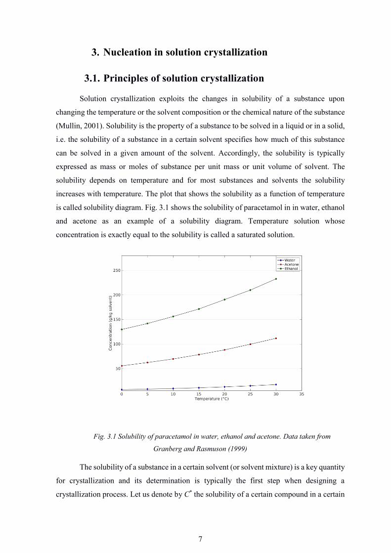
increases with temperature. The plot that shows the solubility as a function of temperature
is called solubility diagram. Fig. 3.1 shows the solubility of paracetamol in in water, ethanol
and acetone as an example of a solubility diagram. Temperature solution whose
concentration is exactly equal to the solubility is called a saturated solution.
Fig. 3.1 Solubility of paracetamol in water, ethanol and acetone. Data taken from
Granberg and Rasmuson (1999)
The solubility of a substance in a certain solvent (or solvent mixture) is a key quantity
for crystallization and its determination is typically the first step when designing a
crystallization process. Let us denote by C* the solubility of a certain compound in a certain

8
solvent. C* in units if [kg/dm3] or [kg/kg] defines the maximum (thermodynamic stable)
concentration of the substance in given amount of solvent. The actual concentration of a
solution with respect to solubility defines the saturation rate, defined as:
𝑆 = 𝐶𝐶∗ 3.1
Were:
C- Actual concentration of solution [kg/dm3]
C*- concentration of saturated solution [kg/dm3]
To start making crystals it is obligatory to transform the solution into a state which
has saturation rate S > 1. This can by, e.g. cooling or the addition of an antisolvent. When
the saturation rate is larger than 1 the solution is in a metastable state, i.e. referred to as
metastable solution. Only when the supersaturation reaches a certain level nucleation sets in
which leads to the formation of solid particles that then grow and deplete the supersaturation.
The region in temperature and solvent composition where a solution is metastable depends
on several factors such as cooling rate and also the mixing, i.e. the stirring speed. For
example, it has been observed that fast cooling often leads to a larger metastable zone. An
empirical explanation for this is that because cooling is quick the energy for nucleation is
taken away from the system and the system remains in the metastable state. In such cases,
to make crystals and start nucleation there is the need to deliver a small amount of energy,
e.g. by shaking the solution or creating some surface roughness on the vessel walls by simply
scratching with a pistil. (Mullin, 2001). It has also been observed that higher stirring speed
makes the metastable zone smaller which empirically can be explained by a similar
argument.
Nucleation is the first step in making crystals. Nucleation describes the process where
few molecules cluster together and form a solid particle that then acts as the seed for crystal
growth. Once these seeds are present, crystal growth continuous until the solution has re-
established saturation, i.e. the molecules that caused the solution to be supersaturated
transformed into the solid. Nucleation may occur spontaneously or it may be induced
artificially. It is not always possible, however, to decide whether a system has nucleated of
its own accord or whether it has done so under the influence of some external stimulus like
be induced by agitation, mechanical shock, friction and extreme pressures within solutions
and melts, as shown by the early experiments of Young (1911) and Berkeley (1912)
9
(Mullin,2015). To make crystals we have to make a clear saturated solution and start cooling
it down to make super saturated solution. As it was mention before excessive supercoiling
does not aid nucleation. There is an optimum temperature for nucleation of a given system,
so if done too fast there will be no nucleation. (Dubrovski, 2005)
3.2. Classification of nucleation phenomena
We distinguish between two main types of nucleation:
1. Primary nucleation
2. Secondary Nucleation
Primary nucleation is further divided into:
1. Homogeneous Nucleation
2. Heterogeneous Nucleation
Primary nucleation occurs when take saturated solution and cool it down slowly to
make a super saturated solution. When it will be cooled down particles, which were
dissolved in to solution, start to exhale from the solution because there is no solvent to react
with the substance of particles. Then because of not enough solvent in solution the molecules
of substance start to be independent particles. When two molecules meet each other
nucleation process begin. Particles, which have been born during nucleation, are called
nucleus, the smallest one are called critical nucleus. Under size of critical molecules there is
no possibility to make a nucleus, which can change to crystals by grooving up. (Myerson,
2002)
Garten and Head suggested that a critical nucleus could be as small as about 10
molecules. A different order of magnitude was proposed by Otpushchennikov (1962), who
estimated the sizes of critical nuclei by observing the behaviour of ultrasonic waves in melts
kept just above their freezing point. For phenol, naphthalene and azobenzene, for example,
he suggested that fewer than 1000 molecules constitute a stable nucleus. It is obvious,
therefore, that there are still some widely diverging views on the question of the size of a
critical nucleus, but this is not surprising as the critical size is super saturation-dependent
which and no consideration is given to this important variable by any of the above authors.
(Mullin, 2001)
10
Secondary nucleation is a state when particles are big enough to split to pieces and
become two or more independent nucleus. Splitting of particles can be done by mechanic
shock or other stresses, which can be involved in fluid in which particles are like mixing or
by hitting wall of system. This state occurs when there is still a supersaturated solution but
there is also a lot of big nucleus, which starts to hit walls of system or a stirrer. When nucleus
hits obstacle and it have enough energy to split then two or more new nucleus appears. When
new nucleus starts to appear they also increase their dimensions by taking new molecules
from supersaturated solution. This process is called crystals grooving. When new nucleuses
are big like they ancestor the whole process make a circle and after several rounds of trial
many new nucleus appears. (Mullin, 2001)
3.3. Classical nucleation theory
The clustering of molecules in a supersaturated solution to form a solid nuclei is
described by the classical nucleation theory, which relates the rate at which nuclei form to
the Gibbs free energy of the nuclei and the supersaturated solution. This leads to the
following expression for the nucleation rate:
𝐽 = 𝑁𝑠𝑍𝑗𝑒𝑥𝑝(−∆𝐺𝑘𝐵𝑇
) 3.2
Where:
∆𝐺 - Gibbs free energy [J]
kBT - thermal energy with T the absolute temperature and kB is the Boltzmann
constant [J]
NS - the number of nucleation sites.
J - Nucleation rate in units of number of nuclei per unit volume per unit time [#/m3
s]
Z - Zeldovich factor Z (essentially the Zeldovich factor is the probability that a
nucleus at the top of the energy barrier will go on to form the new phase instead of dissolving.
(Mullin, 2001).
The Gibbs free energy is made of two contributions, i.e. the energy gain due to the
formation of the new phase and the energy cost due to the formation of a new surface:
11
∆𝐺 = 43𝜋𝑟3𝛥𝑔 + 4𝜋𝑟2𝜎 3.3
Where:
r- Radius of nucleus.
𝛥𝑔- Difference in free energy per unit volume between the thermodynamic phase
nucleation is occurring in, and the phase that is nucleating, which is always negative.
𝜎- Surface tension of the interface between the nucleus and its surroundings, which
is always positive. (Mullin, 2001)
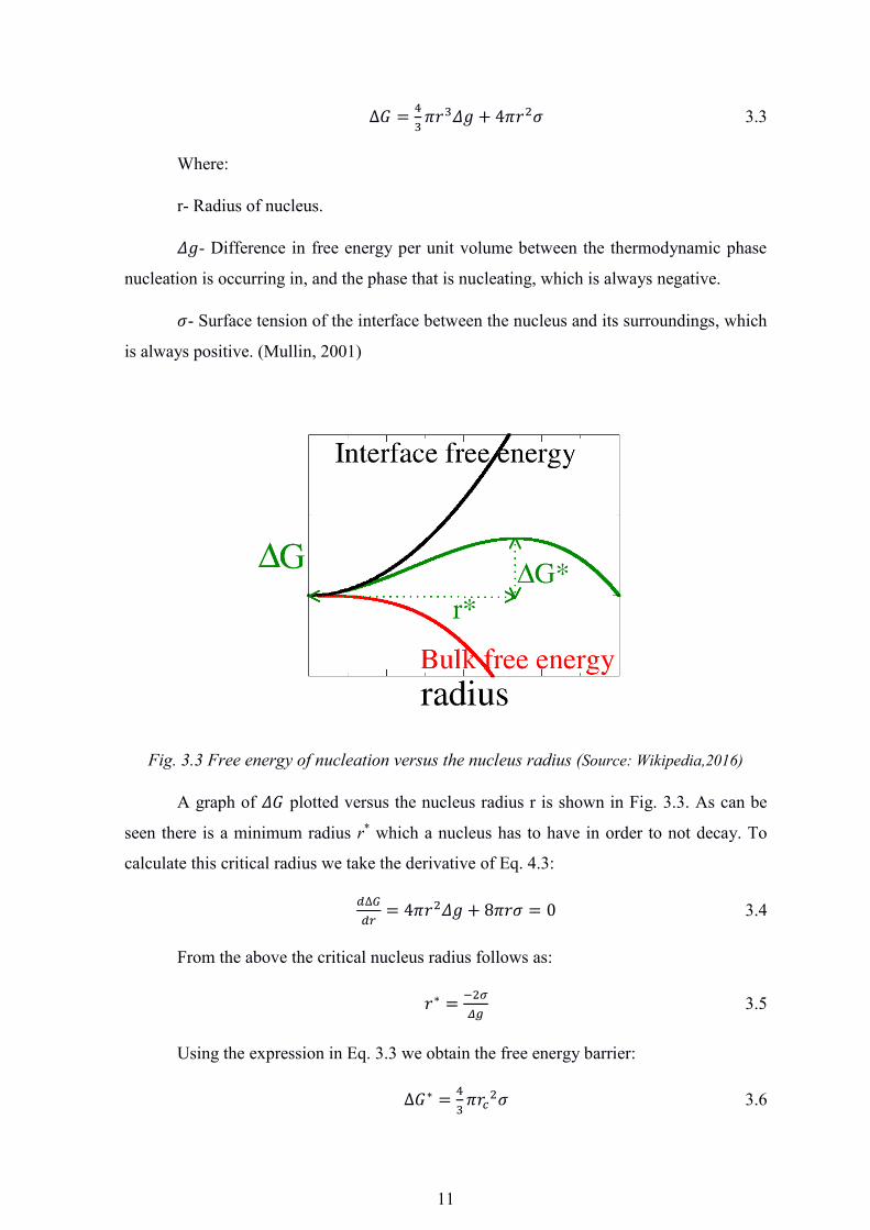
Fig. 3.3 Free energy of nucleation versus the nucleus radius (Source: Wikipedia,2016)
A graph of 𝛥𝐺 plotted versus the nucleus radius r is shown in Fig. 3.3. As can be
seen there is a minimum radius r* which a nucleus has to have in order to not decay. To
calculate this critical radius we take the derivative of Eq. 4.3:
𝑑∆𝐺𝑑𝑟
= 4𝜋𝑟2𝛥𝑔 + 8𝜋𝑟𝜎 = 0 3.4
From the above the critical nucleus radius follows as:
𝑟∗ = −2𝜎𝛥𝑔
3.5
Using the expression in Eq. 3.3 we obtain the free energy barrier:
∆𝐺∗ = 43𝜋𝑟𝑐2𝜎 3.6
12
The surface energy relates to the supersaturation which can be expressed through the
Gibbs-Tomson equation:
𝑙𝑛𝑆 = 2𝜎𝜈𝑘𝐵𝑇𝑟
3.7
Combining the two equations above gives:
∆𝐺𝑐 = 43𝜋 ( 2𝜎𝜈
𝑘𝐵𝑇𝑙𝑛𝑆)2𝜎 = 16𝜋𝜎3𝜈2
3(𝑘𝐵𝑇𝑙𝑛𝑆)2 3.8
Substituting for these expressions in Eq. 3.2 we obtain:
𝐽 = 𝑁𝑠𝑍𝑗𝑒𝑥𝑝 ( −16𝜋𝜎3𝜈2
3(𝑘𝐵𝑇)3(𝑙𝑛𝑆)2) 3.9
Eq. 3.9 is typically referred to a classical nucleation theory. The important aspect to
notice is the dependency of the nucleation rate J on the supersaturation rate S. To highlight
this dependency the literature often uses a lumped expression where the parameters are put
together in two empirical parameters A and B:
𝐽 = 𝐴𝑒𝑥𝑝 ( −𝐵(𝑙𝑛𝑆)2) 3.10
The parameters A and B are characteristic for a given system, i.e. substance and
solvent. (A.S. Myerson, 2002)
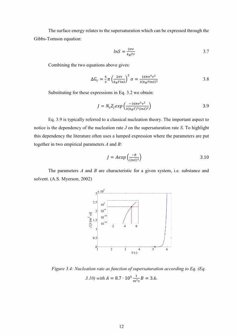
Figure 3.4: Nucleation rate as function of supersaturation according to Eq. (Eq.
3.10) with𝐴 = 8.7 ∙ 105 1𝑚3𝑠
𝐵 = 3.6.
13
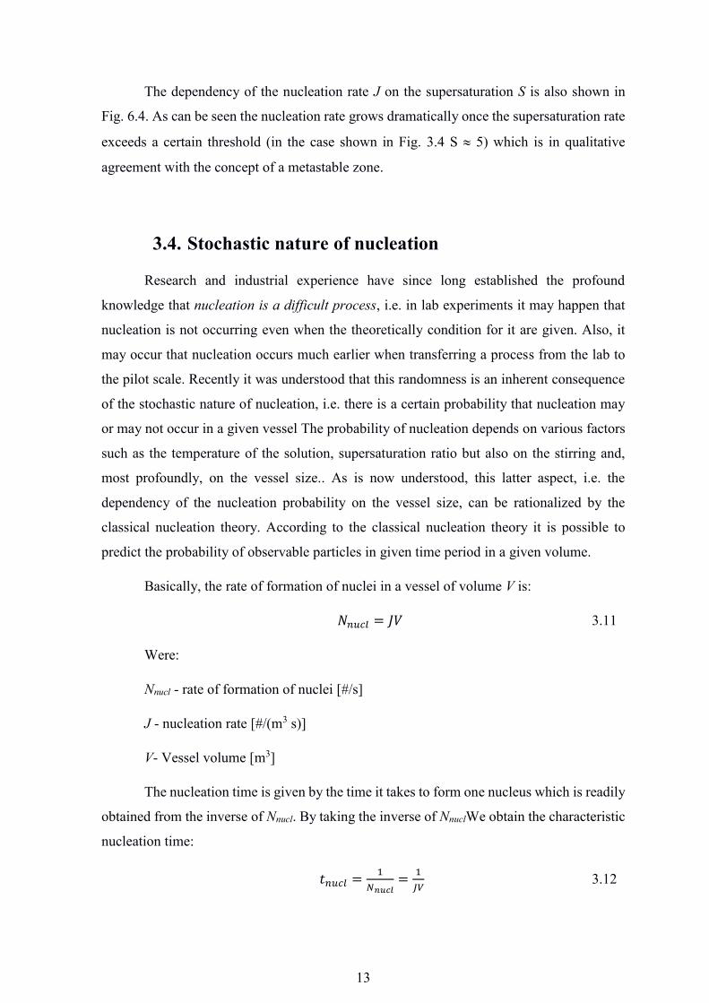
The dependency of the nucleation rate J on the supersaturation S is also shown in
Fig. 6.4. As can be seen the nucleation rate grows dramatically once the supersaturation rate
exceeds a certain threshold (in the case shown in Fig. 3.4 S | 5) which is in qualitative
agreement with the concept of a metastable zone.
3.4. Stochastic nature of nucleation
Research and industrial experience have since long established the profound
knowledge that nucleation is a difficult process, i.e. in lab experiments it may happen that
nucleation is not occurring even when the theoretically condition for it are given. Also, it
may occur that nucleation occurs much earlier when transferring a process from the lab to
the pilot scale. Recently it was understood that this randomness is an inherent consequence
of the stochastic nature of nucleation, i.e. there is a certain probability that nucleation may
or may not occur in a given vessel The probability of nucleation depends on various factors
such as the temperature of the solution, supersaturation ratio but also on the stirring and,
most profoundly, on the vessel size.. As is now understood, this latter aspect, i.e. the
dependency of the nucleation probability on the vessel size, can be rationalized by the
classical nucleation theory. According to the classical nucleation theory it is possible to
predict the probability of observable particles in given time period in a given volume.
Basically, the rate of formation of nuclei in a vessel of volume V is:
𝑁𝑛𝑢𝑐𝑙 = 𝐽𝑉 3.11
Were:
Nnucl - rate of formation of nuclei [#/s]
J - nucleation rate [#/(m3 s)]
V- Vessel volume [m3]
The nucleation time is given by the time it takes to form one nucleus which is readily
obtained from the inverse of Nnucl. By taking the inverse of NnuclWe obtain the characteristic
nucleation time:
𝑡𝑛𝑢𝑐𝑙 = 1𝑁𝑛𝑢𝑐𝑙
= 1𝐽𝑉
3.12
14
For example, nucleation rates for the system m-aminobezoic acid water/ethanol (m-
ABA) solutions were measured experimentally by Jiang and Ter Hoorst (2010) and
nucleation rate parameters A and B were derived. Using their values, i.e. 𝐴 = 8.7 ∙
105 1𝑚3𝑠
𝐵 = 3.6, in combination with Eq. 6.10 we calculate that the system m-ABA in
water/ethanol at a supersaturation rate of S=1.5 exhibits:
𝐽 = 4.03 ∙ 10−4 1𝑚3𝑠
3.13
Considering a small vial of volume is V = 1 ml, we find that the number of nuclei per
second is:
Nnucl = 4.03 ∙ 10−10 1s 3.14
From the above the characteristic nucleation time is:
tnucl = 2.5 ∙ 105s 3.15
Eq. 3.15 gives the average time it takes to form one nucleus in a vessel of volume
V = 1 ml. However, because of the stochastic nature of the nucleation phenomenon this first
nucleus may pop into existence earlier or later than tnucl, i.e. there is a certain probability for
the time at which the first nucleus pops into existence, with the expected value given by tnucl
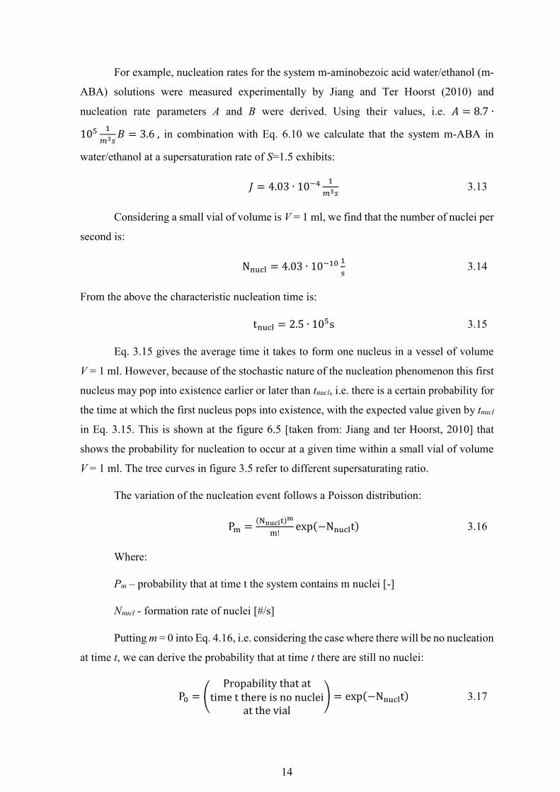
in Eq. 3.15. This is shown at the figure 6.5 [taken from: Jiang and ter Hoorst, 2010] that
shows the probability for nucleation to occur at a given time within a small vial of volume
V = 1 ml. The tree curves in figure 3.5 refer to different supersaturating ratio.
The variation of the nucleation event follows a Poisson distribution:
Pm = (Nnuclt)m
m!exp(−Nnuclt) 3.16
Where:
Pm – probability that at time t the system contains m nuclei [-]
Nnucl - formation rate of nuclei [#/s]
Putting m = 0 into Eq. 4.16, i.e. considering the case where there will be no nucleation
at time t, we can derive the probability that at time t there are still no nuclei:
P0 = (Propabilitythatat
timetthereisnonucleiatthevial
) = exp(−Nnuclt) 3.17
15
Figure 3.5 Probability of nucleation taken from Jiang and ter Hoorst, (2010)
Vice-versa, if the probability that there is no nuclei at time t is given by P0 above,
the probability that there is at least one nuclei at time t is:
P≥1 = (Propabilitythatat
timetthereisatleastonenucleiatthevial
) = 1 − exp(−Nnuclt) 3.18
Substituting Nnucl we obtain:
P≥1 = 1 − exp(−JVt) 3.19
Because there is always delay between appearing first nuclei and time of it visibility
so it is necessary to make a patch in the above equation, using tg as the time of first seen the
nuclei. By including this patch we arrive at our final probability function for nucleation to
occur at time t:
P≥1(t) = 1 − exp (−JV(t − tg)) 3.20
From equation above it can be easily deduced that probability of nucleation is
connected to time, volume of fluid and the nucleation rate J. In most of systems volume of
fluid and J factor are constants limitation of increasing probability of nucleation is tg as a
time of first seen the nuclei.
16
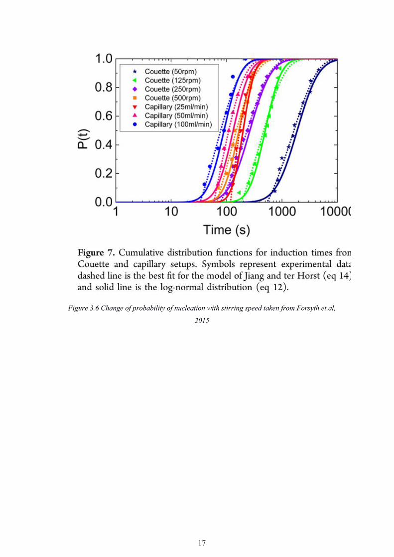
3.5. Influence of stirring on nucleation
Enhancement of nucleation by stirring is a well-known phenomenon in solution
crystallization [Forsyth et.al, 2015]. However the reason for this enhancement and
underlying mechanism are not well understood. A common explanation is that the fluid shear
generated by the stirrer breaks up some kind of pre-nuclei which harms large nuclei to
fragments, which then act as a nuclei induce crystallization. Another explanation in that
stirring improves the mixing rate and therefore the mass brakes, making it easier for the
molecules to come together and form a cluster that then developed into nuclei.
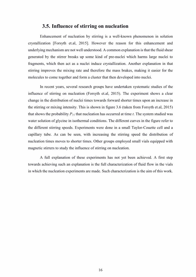
In recent years, several research groups have undertaken systematic studies of the
influence of stirring on nucleation (Forsyth et.al, 2015). The experiment shows a clear
change in the distribution of nuclei times towards forward shorter times upon an increase in
the stirring or mixing intensity. This is shown in figure 3.6 (taken from Forsyth et.al, 2015)
that shows the probability P≥1 that nucleation has occurred at time t. The system studied was
water solution of glycine in isothermal conditions. The different curves in the figure refer to
the different stirring speeds. Experiments were done in a small Taylor-Couette cell and a
capillary tube. As can be seen, with increasing the stirring speed the distribution of
nucleation times moves to shorter times. Other groups employed small vials equipped with
magnetic stirrers to study the influence of stirring on nucleation.
A full explanation of these experiments has not yet been achieved. A first step
towards achieving such an explanation is the full characterization of fluid flow in the vials
in which the nucleation experiments are made. Such characterization is the aim of this work.
17
Figure 3.6 Change of probability of nucleation with stirring speed taken from Forsyth et.al,
2015

18
Computational Fluid Dynamic (CFD) for millilitre
vial. According to the experiments made by Joop her Host and others there can be
correlation a between the speed of stirring and the nucleation. There is a hypothesis that the
nucleation is observed in the experiments is actually a kind of secondary nucleation occurs
because particles hits or pass nearly stirrer and break up.
To confirm that hypothesis CFD has been used to analyse the flow in the millilitre
vial. To make the simulation a 3D model of the considered system and in next step was to
make a mesh on it. After making mesh there has been simulation of varies stirring speed to
obtain velocity flow fields. From velocity flow fields it has been made contour plots to check
influence of different boundary conditions and a model used for calculation.
4.1. Computational Fluid Dynamic and turbulent model
To calculate the flow field in Computational Fluid Dynamic (CFD) there exsist many
models and variations of these models. Fluid flow field is mostly described by Navier–
Stokes and Continuity equations. Navier–Stokes equations for an incompressible fluid can
be presented as (Pope 2000):
𝜌 (𝜕�⃗� 𝜕𝑡
+ (𝑣 ∙ ∇)𝑣 ) = 𝜌𝑓 − ∇𝑝 + 𝜇∆�⃗� 4.1
Where:
ρ -density of fluid [kg/m3]
𝑓 -Vector representing external forces [N/kg]
𝑣 -Speed in one direction [m/s]
μ- Kinematic viscosity [kg/m s]
p- Pressure gradient [Pa]
Δ-Laplace operator
∇- Del
t- Time [s]
The Navier-Stokes equation in realistic geometries can be solved only by numerical
methods and even this often calls for some compromise, in example the form of turbulent
19
models. Solving analytically Navier–Stokes equations has been obtained as one of 8
millennium problems for which solving has been set up price one million of US Dollars.
Until today this problem is solved only analytically for basic fluid flow fields that are mostly
one dimensions fluid flow fields.
To solve fluid flow filed it is also used Continuity equation, which describe the flow
in continuous medium and it has been defined as (Pope 2000):
𝜕𝜌𝜕𝑡
+ ∇ ∙ (𝜌𝑣 ) = 0 4.2
The most common models to solve Navier–Stokes equations are laminar model and
models which use Reynolds-averaged Navier–Stokes equations such as k- ε, k-ω, SST or
Reynolds stress equation model.
Solving Navier–Stokes and Continuity equations by CFD are based on fine volume
method which is based on Euler fluid dynamic system. In Euler fluid dynamic it has been
obtained that there is a specific point which position in the system is constant and fluid flows
though this point. Theoretically this point has indefinite small dimensions that are very close
to 0, but not there are different than 0 (Pope 2000).
Fine volume methods realize Euler fluid dynamic by dividing the system volume in
to small volumes called cells. Dividing the system volume to small volumes is called
meshing, and divided the system is called mesh. Mesh can be made from tetrahedrons or
hexahedrons. Smaller dimensions of the tetrahedrons or the hexahedrons results in higher
calculation accuracy but also slow down calculation speed (Wendt and Anderson 2009).
In every specific cell calculations for fluid flow field are made using model
equations. Calculations were made in centre points of cells and values on edges are checked
with neighbour’s cells. Difference of parameters between cells calculation is has been
summed up and displayed as a convergence level of calculated parameter like x,y,z-
velocities, Continuity equation and other model equations (Wendt and Anderson 2009).
The laminar model solves numerically Navier–Stokes and Continuity equations
based on assumption that flow is laminar so there are no turbulences and velocity gradient
is based on laminar flow, so volume viscosity is 0 because fluid is incompressible and also
kinetic viscosity is predicted to be constant. Liquid is passing by speed on the basis of
interaction viscous (Wendt and Anderson 2009).

20
Reynolds-averaged Navier–Stokes equations models are based on Reynolds
decomposition which can be presented as (Pope 2000):
a(t) = a̅ + a´(t) 4.3
Where
a(t)- property value at time t
a̅- Average property value
a´(t)- fluctuation of property, which is time dependent.
Reynolds-averaged Navier–Stokes equations for stationary, incompressible
Newtonian fluid for two dimensions flow can be writhed as (Pope 2000):
ρu�̅�∂ui̅̅̅∂xj
= ρfi̅ +∂
∂xj[−p̅δij + μ (∂ui̅̅̅
∂xj+ ∂uj̅̅̅
∂xi) − ρu´iu´j̅̅ ̅̅ ̅̅ ̅] 4.4
The Reynolds decomposition allows solving Reynolds-averaged Navier–Stokes
equations in time independent state and then calculating fluctuation values using Reynolds
operator when it is needed. For solving standard velocity fluctuations it has been used the
Boussinesq eddy viscosity hypothesis (Boussinesq 1877), which says that:
u´iu´j̅̅ ̅̅ ̅̅ ̅ = 23kδij − μm (∂ui̅̅̅
∂xj+ ∂uj̅̅̅
∂xi) 4.5
Where:
μm-Turbulent eddy viscosity ratio.
Turbulent eddy viscosity ratio can be calculated from model equation:
μm = ρCμ𝑘2
ε 4.6
Where:
Cμ = 0.09- Constant.
k- Turbulent kinetic energy
ε- Energy dissipation rate
One of ways to solve Reynolds-averaged Navier–Stokes equations it has been
solving k- ε model with solve numerically equations for k and ε.
21
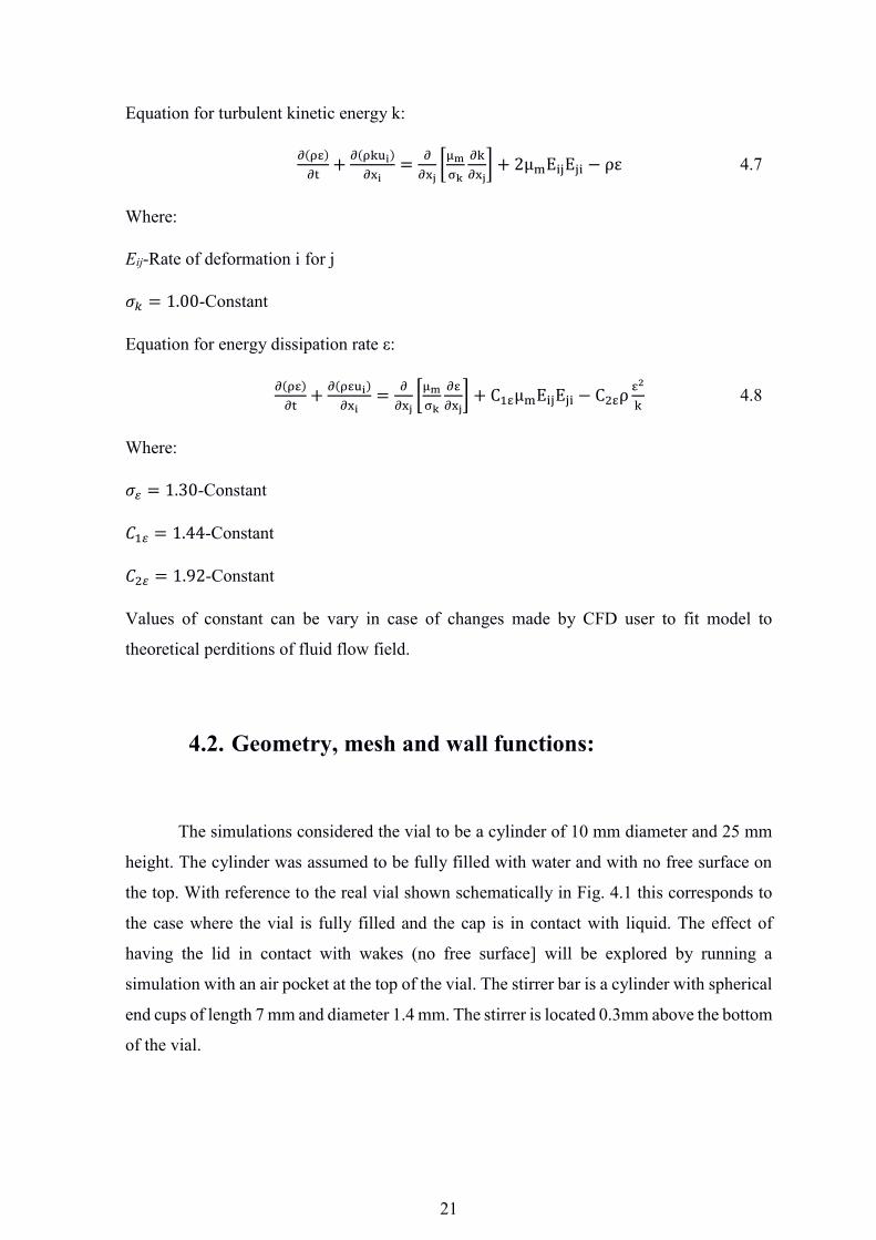
Equation for turbulent kinetic energy k:
∂(ρε)∂t
+ ∂(ρkui)∂xi
= ∂∂xj
[μmσk
∂k∂xj
] + 2μmEijEji − ρε 4.7
Where:
Eij-Rate of deformation i for j
𝜎𝑘 = 1.00-Constant
Equation for energy dissipation rate ε:
∂(ρε)∂t
+ ∂(ρεui)∂xi
= ∂∂xj
[μmσk
∂ε∂xj
] + C1εμmEijEji − C2ερε2
k 4.8
Where:
𝜎𝜀 = 1.30-Constant
𝐶1𝜀 = 1.44-Constant
𝐶2𝜀 = 1.92-Constant
Values of constant can be vary in case of changes made by CFD user to fit model to
theoretical perditions of fluid flow field.
4.2. Geometry, mesh and wall functions:
The simulations considered the vial to be a cylinder of 10 mm diameter and 25 mm
height. The cylinder was assumed to be fully filled with water and with no free surface on
the top. With reference to the real vial shown schematically in Fig. 4.1 this corresponds to
the case where the vial is fully filled and the cap is in contact with liquid. The effect of
having the lid in contact with wakes (no free surface] will be explored by running a
simulation with an air pocket at the top of the vial. The stirrer bar is a cylinder with spherical
end cups of length 7 mm and diameter 1.4 mm. The stirrer is located 0.3mm above the bottom
of the vial.

22
Figure 4.1. HPLC vial considered in this work- dimensions in mm.

23
Figure 4.2. HPLC vial considered in this work: Photograph
The meshing of the cylindrical vial and the stirrer is done with 510,000 grid cells
comprising two types of cells, i.e. hexahedrons and tetrahedrons. The parameters of mesh
are given in Table 4.1. The mesh was generated with an element size of 0.18 mm for the
tetrahedrons and 0.3 mm for hexahedrons, with inflation on the side wall, the bottom, the
surface and at the stirrer.
Parameter of mesh were enough to run simulation and get mostly convergence in
level lower than 10-5 for velocity and continuity equations, but for specific model equations
it has been mostly reached convergence level at 10-7-10-8.
Table 4.1- Parameters of mesh
Mesh Metric Minimum Average Maximum
Orthogonal quality 0.24567 0.92927 1
Skewness 2.241×10⁻⁵ 0.17055 0.84956
Element quality 0.02841 0.74501 1
24
The boundary conditions of the simulation were set up as following:
1. The whole system is moving as a rotation frame option with the rotation speed of the
impeller.
2. Sidewalls, bottom wall and upper surface are simulated as solid wall.
3. From the perspective of the moving frame all solid walls are moving.
4. The vial is filled up by water which temperature is 20°C.
5. The stirrer is a stationary wall within the rotary frame.
6. No heat transfer.
7. The stirrer does not have any mass
8. The roundness corners of vial are not important for fluid flow.
The above boundary conditions where used based on theoretical perditions of fluid flow
parameters and the Author experiences with CFD. Using a rotary frame allows for simulating
full mass fluid forces and by rotating wall in opposite direction it has been obtained not
moving walls. It has been also assumed that rotary speed of fluid is the same as speed of
stirring.
4.3. Investigating the Reynolds number.
To investigate whether the flow is turbulent or laminar it has been recently used the
Reynolds Number was considered for a stirred vessel, Reynolds number is defined as:
𝑅𝑒 = 𝑑2𝜋𝜔𝜈
4.9
Where:
d=0.007 [m] - diameter of magnetic impeller.
ω- Rotation speed [rad/s]
ν= 9.79×10⁻⁷ [m2/s] -kinematic viscosity of water in 20°C
For this system Reynolds criteria are not well known but for similar dimensions
reactor by Hortsch et. al (2010) it has been proposed that flow is strictly turbulent when
25
Reynolds number is above 3000 and before reaching this number is predicted that flow will
start to be transient. Hortsch et. al. (2010) used milliliter-scale bioreactor which has 12ml
volume and d/D = 0.7, H/D = 2, and w/D = 0.1
The considered here vial has following parameters d/D=7, H/D=2.5 and w/d=0.1.
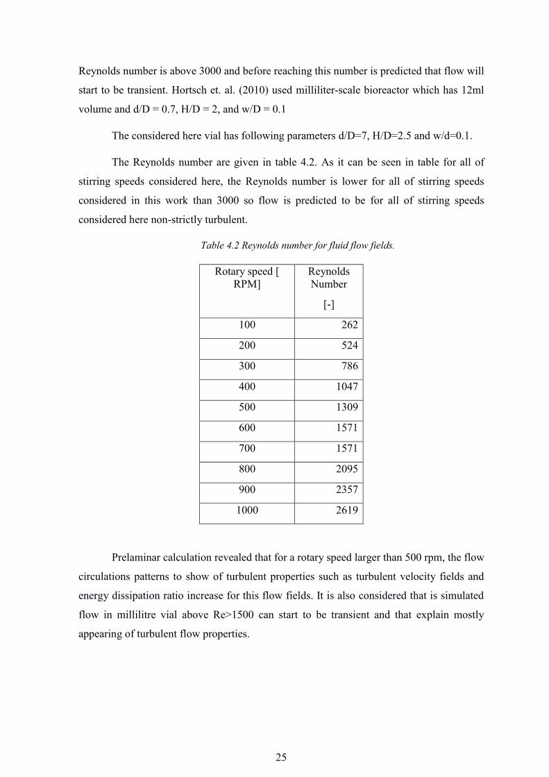
The Reynolds number are given in table 4.2. As it can be seen in table for all of
stirring speeds considered here, the Reynolds number is lower for all of stirring speeds
considered in this work than 3000 so flow is predicted to be for all of stirring speeds
considered here non-strictly turbulent.
Table 4.2 Reynolds number for fluid flow fields.
Rotary speed [ RPM]
Reynolds Number
[-]
100 262
200 524
300 786
400 1047
500 1309
600 1571
700 1571
800 2095
900 2357
1000 2619
Prelaminar calculation revealed that for a rotary speed larger than 500 rpm, the flow
circulations patterns to show of turbulent properties such as turbulent velocity fields and
energy dissipation ratio increase for this flow fields. It is also considered that is simulated
flow in millilitre vial above Re>1500 can start to be transient and that explain mostly
appearing of turbulent flow properties.

26
4.4. CFD simulation parameters
For simulating fluid flow it has been used ANSYS Fluent 16.2 release based on
Windows 8.1 x64 desktop machine. Machine has Intel Core i7-4790 CPU with 3.6GHz clock
signal with 4 cores and 8 logical issues operating on 32GB of RAM memory. Simulations
were made using parcel processing based on 8 logical issues, which speed up calculations
and make calculation process in acceptable time.
It has been done many various flow field simulations on two models laminar and k-
ε, run schema of simulation is shown in table 4.3. Crossed box stands for made simulation
which has reach enough level of convergence up to 10-8.
Table 4.3Run schema of simulation runs in ANSYS Fluent 16.2 release
Stirring speed [rpm]
100 200 300 400 500 600 700 800 900 1000
k-ε model
Laminar model
For k-ε simulation it has been used RGN model in Swirl Dominated Flow mode,
which simulate Coriolis body force. It has been used standard wall functions with Full
Buoyancy Effects and Curvature Correction mode, which helps to get better convergence
level.
For both models has been used SIMPLE solving scheme with second order upwind
solution method with High Order Term Relaxation to improve results of calculation.
Solution is based on pressure-based solver with absolute velocity formulation in mostly time
steady mode. To check influence of free surface on simulation parameters has been used
time transient mode for 1000 rpm with 0.001s time step simulating 200 time steps.
From obtained data from fluid flow simulation it has been selected to present most
important flow fields for 100, 300, 600 and 1000 rpm. Other fluid flow simulations were
used to discover correlation between fluid flow average properties such as kinetic energy,
dissipation rate, power input or power number and speed of stirring.
27
CFD results:
5.1. Comparing flow models
To choose suitable model for CFD simulation it has been made two simulations using
different models (laminar and k-ε) to check which model will give the results that best fits
to theoretical predictions and gives the most symmetrical velocity field in section plane
which goes across stirrer in vertical plane. From previous literature and theoretical studies
flow in small cylinder is expected to be symmetrical in vertical and horizontal section planes.
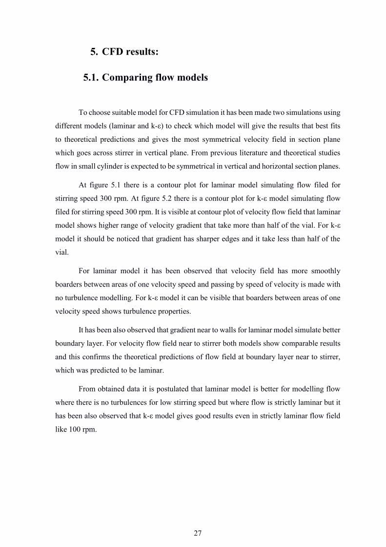
At figure 5.1 there is a contour plot for laminar model simulating flow filed for
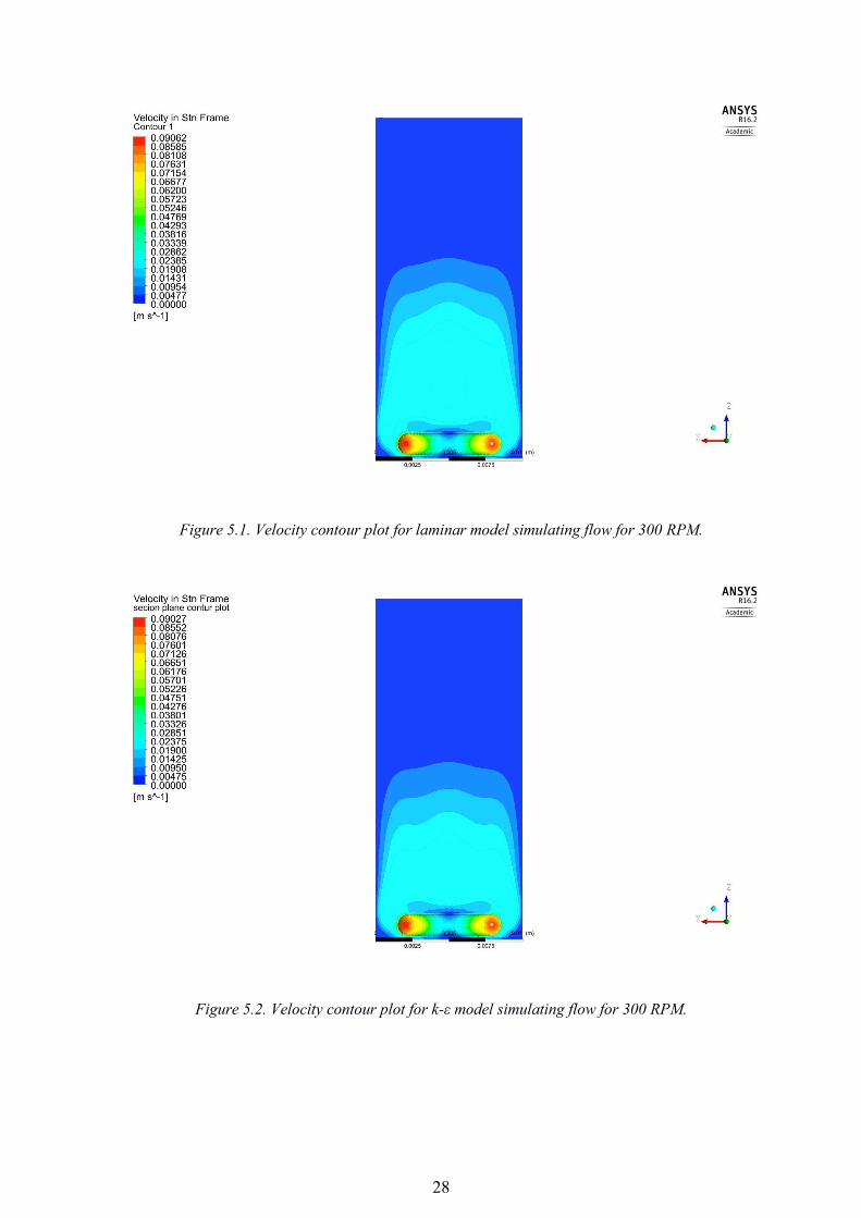
stirring speed 300 rpm. At figure 5.2 there is a contour plot for k-ε model simulating flow
filed for stirring speed 300 rpm. It is visible at contour plot of velocity flow field that laminar
model shows higher range of velocity gradient that take more than half of the vial. For k-ε
model it should be noticed that gradient has sharper edges and it take less than half of the
vial.
For laminar model it has been observed that velocity field has more smoothly
boarders between areas of one velocity speed and passing by speed of velocity is made with
no turbulence modelling. For k-ε model it can be visible that boarders between areas of one
velocity speed shows turbulence properties.
It has been also observed that gradient near to walls for laminar model simulate better
boundary layer. For velocity flow field near to stirrer both models show comparable results
and this confirms the theoretical predictions of flow field at boundary layer near to stirrer,
which was predicted to be laminar.
From obtained data it is postulated that laminar model is better for modelling flow
where there is no turbulences for low stirring speed but where flow is strictly laminar but it
has been also observed that k-ε model gives good results even in strictly laminar flow field
like 100 rpm.
28
Figure 5.1. Velocity contour plot for laminar model simulating flow for 300 RPM.
Figure 5.2. Velocity contour plot for k-ε model simulating flow for 300 RPM.
29
5.2. Influence of stirring speed in fluid flow
To investigate the fluid flows properties in the millilitre vial have been made analyse
to check changes made by increasing the speed of stirring. It has been chosen to compare
four different speeds of stirring namely 100,300,600 and 1000 rpm. For all of these stirring
speeds, the velocity field, represented as contour and vector plots in section plane which
goes across stirrer where analysed. It has been also investigated turbulent energy dissipation
rate and kinetic turbulent energy by making contour plots section plane which goes across
stirrer.
Figure 6.3 shows the velocity contour plot for velocity flow field generated by 100
rpm while figure 5.4 shows the velocity contour plot at 300 rpm stirring speed. Likewise, in
figure 5.5 there is a velocity contour plot for velocity flow field generated by 600 rpm stirring
speed, while in figures 5.6 there is a velocity contour plot for velocity flow field generated
by 1000 rpm stirring speed.
At figures 5.7 there is a velocity vector plot for velocity flow field generated by 100
rpm stirring speed. At figures 5.8 there is a velocity vector plot for velocity flow field
generated by 300 rpm stirring speed. At figures 5.9 there is a velocity contour plot for
velocity flow field generated by 600 rpm stirring speed. At figure 5.10 there is a velocity
vector plot for velocity flow field generated by 1000 rpm stirring speed.
It has been observed that with increasing the stirring speed non-zero flow filed starts
to climb up from nearly the bottom of the millilitre vial for 100 rpm to nearly the top of the
millilitre vial for 1000 rpm. It has been also observed that for 100 rpm the flow makes only
non-zero velocity near to centre and tips of the stirrer, while the area in middle stays has near
to zero velocity. For 300 rpm stirring speed it has been noticed that there is also low velocity
field near to top of stirrer and near to centre there is zero velocity area. For 600 rpm stirring
speed it has been pointed out that low velocity field replaces this zero velocity filed with
zero velocity up from centre of the stirrer. For 1000 rpm it has been noticed that there are
only some points of zero velocity at the middle in the area near to stirrer and they are
predicted to be numerical errors but from obtained data it is impossible judge if it an
numerical error or place were velocity is near to zero in real flow field because of
turbulences.

30
Figure 5.3 Velocity contour plot for flow for 100 RPM.
Figure 5.4. Velocity contour plot for flow for 300 RPM.

31
Figure 5.5 Velocity contour plot for flow for 600 RPM.
Figure 5.6 Velocity contour plot for flow for 1000 RPM.

32
Figure 5.7 Velocity vector plot for flow for 100 RPM.
Figure 5.8 Velocity vector plot for flow for 300 RPM.
33
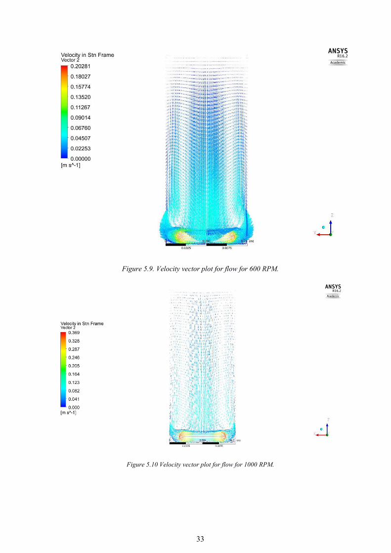
Figure 5.9. Velocity vector plot for flow for 600 RPM.
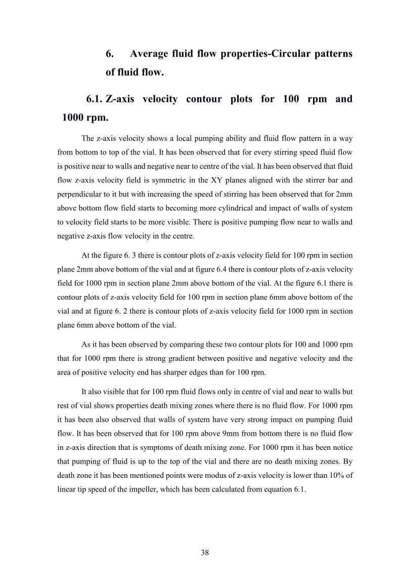
Figure 5.10 Velocity vector plot for flow for 1000 RPM.

34
For 100 rpm fluid flow field has only developed in few areas of the millilitre vial and
comparing to other rotary speed it not well developed in rest of the vial. It should be also
observed that 300 rpm fluid flow field is fully developed, but it upper half of millilitre vial
is have velocity near to zero. For 600 rpm fluid flow field stats to fill up whole volume of
the vial. It has been also pointed out that for 1000 rpm shape of velocity flow field is also
result of influence of top the millilitre vial.
From vector plots it is clearly visible that generally fluid circulation pattern is from
walls and bottom to the top of the vial where fluid stars to goes down and reach stirrer in the
symmetry axis of the millilitre vial. It has been observed that for speed of stirring 100 rpm
at section plane there are only small round eddies, which are located near to top of stirrer. It
should be also observed that for speed of stirring 100 rpm fluid splash only on small part of
the walls not higher than approximately 2mm above the centre of stirrer. There is also at the
corners of the vial 0 velocity zone in which fluid is stays unmoved.
It has been also noticed that with increasing speed of stirring shape of main eddies
changes and become more elliptical. For 100 rpm main eddies are nearly circular. For 300
rpm main eddies start to be elliptical but their shape is still nearly to be circular. At stirring
speed 600 rpm eddies became fully elliptical and start to twist to sides of the millilitre vial.
Vector plots shows also that pumping route start to be longer, as it has been mention
before, but it keep still the horizontal dimensions of eddies. For 300 rpm velocity vector
plots shows that small eddies for 100 rpm starts to become lager with increasing the stirring
speed. It should be noticed that with increasing the stirring speed fluid is still not good mixed
at lower corners of the vial. However for stirring speed 600 rpm it is visible that at the corners
of the vial starts to make small eddies, which mix fluid properly, which expand with
increasing the stirring speed and for 1000 rpm they are good develop comparing to 100 rpm.
From obtained data it is clearly seen that eddies at the corners of millilitre vial should
be consider as turbulent boundary layer, which grow up with increasing stirring speed, and
for stirring speed below 300 rpm boundary layer is strictly laminar.

35
5.3. Influence of free surface for boundary conditions
As it has been mention before one of boundary conditions was that, upper surface of
the fluid was simulated as a wall. This boundary condition has been realized in assumption
that there is no significant influence of free surface on rotary flow because most of fluid flow
were predicted to be laminar. As it has been observed for most stirring speeds fluid flow
field does not reach top of the vial and fluid flow is realized more than 2mm above upper
surface of the fluid. Only for starring speed 1000 rpm it has been observed that fluid flow
field ends nearly to top of the vial and made assumption can have an influence to fluid flow
field.
To check possibility of influence of boundary conditions to fluid flow field for 1000
rpm it has been made an experiment for 1000 rpm. Vial from figure 4.2 has been filed up
with water up to the top and stirred with a magnetic stirrer and photographed with a stirring
and without stirring to present influence of the stirring to free surface (Fig.5.11). Than water
has been taken out using microliter pipette 200µL up to 800 µL and experiment was run
again (Fig.5.12).
As it has been observed from experiment at figure 5.11 that there bigger impact for
free surface for all of experiments has surface tension and capillary forces than stirring. From
figure 5.12 it has been observed that fluid goes up approximately not more than 1 mm and
upper surface of liquid goes down not more than 1mm and still capillary forces has a bigger
impact on free surface than stirring. Shape of free surface has been observed as nearly
parabolic and mostly at the centre of the millilitre vial even without stirring. It has been also
observed that shape of free surface has no collision with contours of velocity flow field. It
should be also reminded that model of the vial assumed that is fully filed with a liquid and
this correspond to first series of experiment.
From observations which has been made at experiment on free surface for stirring
speed 1000 rpm it has been assumed that using boundary condition of wall to replace free
surface was correct and the influence of free surface should be investigated only above 1000
rpm, but it is strongly recommended to check first influence of free surface on fluid flow
field and after that is recommended to run simulation in time steady state to speed up
calculations and obtain better results, especially better level of convergence.

36
Viall stirred Viall unstirred
Figure 5.11 Influence of stirring to of free surface at vial filed up until top.

37
Viall stirred Viall unstirred
Figure 5.11 Influence of stirring to of free surface at vial with reduced
volume
38
Average fluid flow properties-Circular patterns
of fluid flow.
6.1. Z-axis velocity contour plots for 100 rpm and
1000 rpm.
The z-axis velocity shows a local pumping ability and fluid flow pattern in a way
from bottom to top of the vial. It has been observed that for every stirring speed fluid flow
is positive near to walls and negative near to centre of the vial. It has been observed that fluid
flow z-axis velocity field is symmetric in the XY planes aligned with the stirrer bar and
perpendicular to it but with increasing the speed of stirring has been observed that for 2mm
above bottom flow field starts to becoming more cylindrical and impact of walls of system
to velocity field starts to be more visible. There is positive pumping flow near to walls and
negative z-axis flow velocity in the centre.
At the figure 6. 3 there is contour plots of z-axis velocity field for 100 rpm in section
plane 2mm above bottom of the vial and at figure 6.4 there is contour plots of z-axis velocity
field for 1000 rpm in section plane 2mm above bottom of the vial. At the figure 6.1 there is
contour plots of z-axis velocity field for 100 rpm in section plane 6mm above bottom of the
vial and at figure 6. 2 there is contour plots of z-axis velocity field for 1000 rpm in section
plane 6mm above bottom of the vial.
As it has been observed by comparing these two contour plots for 100 and 1000 rpm
that for 1000 rpm there is strong gradient between positive and negative velocity and the
area of positive velocity end has sharper edges than for 100 rpm.
It also visible that for 100 rpm fluid flows only in centre of vial and near to walls but
rest of vial shows properties death mixing zones where there is no fluid flow. For 1000 rpm
it has been also observed that walls of system have very strong impact on pumping fluid
flow. It has been observed that for 100 rpm above 9mm from bottom there is no fluid flow
in z-axis direction that is symptoms of death mixing zone. For 1000 rpm it has been notice
that pumping of fluid is up to the top of the vial and there are no death mixing zones. By
death zone it has been mentioned points were modus of z-axis velocity is lower than 10% of
linear tip speed of the impeller, which has been calculated from equation 6.1.

39
𝑢𝑡𝑖𝑝𝑖 = 𝜋𝑑𝑖𝑚𝑝𝑒𝑙𝑙𝑒𝑟𝑖
60 𝑠𝑚𝑖𝑛
= {𝑓𝑜𝑟𝑖 = 100𝑟𝑝𝑚𝑢𝑡𝑖𝑝100 = 0.37𝑓𝑜𝑟𝑖 = 1000𝑟𝑝𝑚𝑢𝑡𝑖𝑝1000 = 3.7 6.1
Figure 6. 1 Contour plots of z-axis velocity field for 100 rpm in section plane 6mm above bottom
of the vial.
Figure 6.2 Contour plots of z-axis velocity field for 100 rpm in section plane 6mm above bottom of the vial.

40
Figure 6. 3 Contour plots of z-axis velocity field for 1000 rpm in section plane 2mm above bottom of the vial.
Figure 6.4 Contour plots of z-axis velocity field for 100 rpm in section plane 2mm above bottom of the vial.

41
From plots of z-axis velocity on 6mm above bottom it is visible that flow start to be
cylindrical at 2mm above bottom and become fully cylindrical for 1000 rpm and elliptical
for 100 rpm at 6mm above bottom. For 100 rpm it is postulated that the influence of
cylindrical shape of stirrer make fluid flow field elliptical for 6mm above bottom. It the
lower parts of the vial it flow pattern still shows position of the impeller, well far away it
become symmetric.
For 1000 rpm is postulated that for cylindrical shape of fluid flow is responsible
shape of walls of the vial. It has been also observed that boundary conditions for 1000 rpm
has influence on fluid z-axis velocity flow field and it to propound that boundary layer is
smaller than is show on the contour plot.
From this observation it been assumed that with increasing speed of stirring influence
of shape stirrer to fluid z-axis velocity flow field decreases and wall influence has been
increasing. It has been also noticed that with increasing the stirring speed death zones starts
to decreases and start higher from a bottom of the vial.
6.2. Positive z-axis velocity investigation:
In order to qualify the circulation pattern in the vial it has been investigated the
positive z-axis velocity. It is predicted that responsible for secondary nucleation in such
system is mostly collisions with walls or sitter. The positive z-axis velocity is defined as:
𝑉+ = {𝑉𝑧𝑖𝑓𝑉𝑧 > 00𝑖𝑓𝑉𝑧 ≤ 0 6.2
It should be also pointed out that positive z-axis velocity does not show different
between negative fluid flow and death zones or zero z-axis velocity. It has to be noticed that
for normal z-axis velocity surface average should be 0, but because of numerical error of
simulation in CFD could be different than 0.
Positive z-axis velocity is important to quantify the fluid flow circulation inside the
vial. The circulation of the fluid from the intensely mixed region close to the calm region in
the uppers parts of the vial is believed to provide an explanation for the influence of stirring
on nucleation.
From V+ function it has been generated surface average for 11 section planes located
from 2 to 22 millimetres above bottom, section plane are distanced 2 mm from each other.
42
Values of positive z-axis velocity are presented in table 6.1 and also at figure .6.5. Surface
average is defined as:
⟨𝑉+⟩ = 1𝑆 ∮ 𝑉+ 𝑑𝑆
𝑆 6.3
Where:
S- Cross section area
dS- Surface element
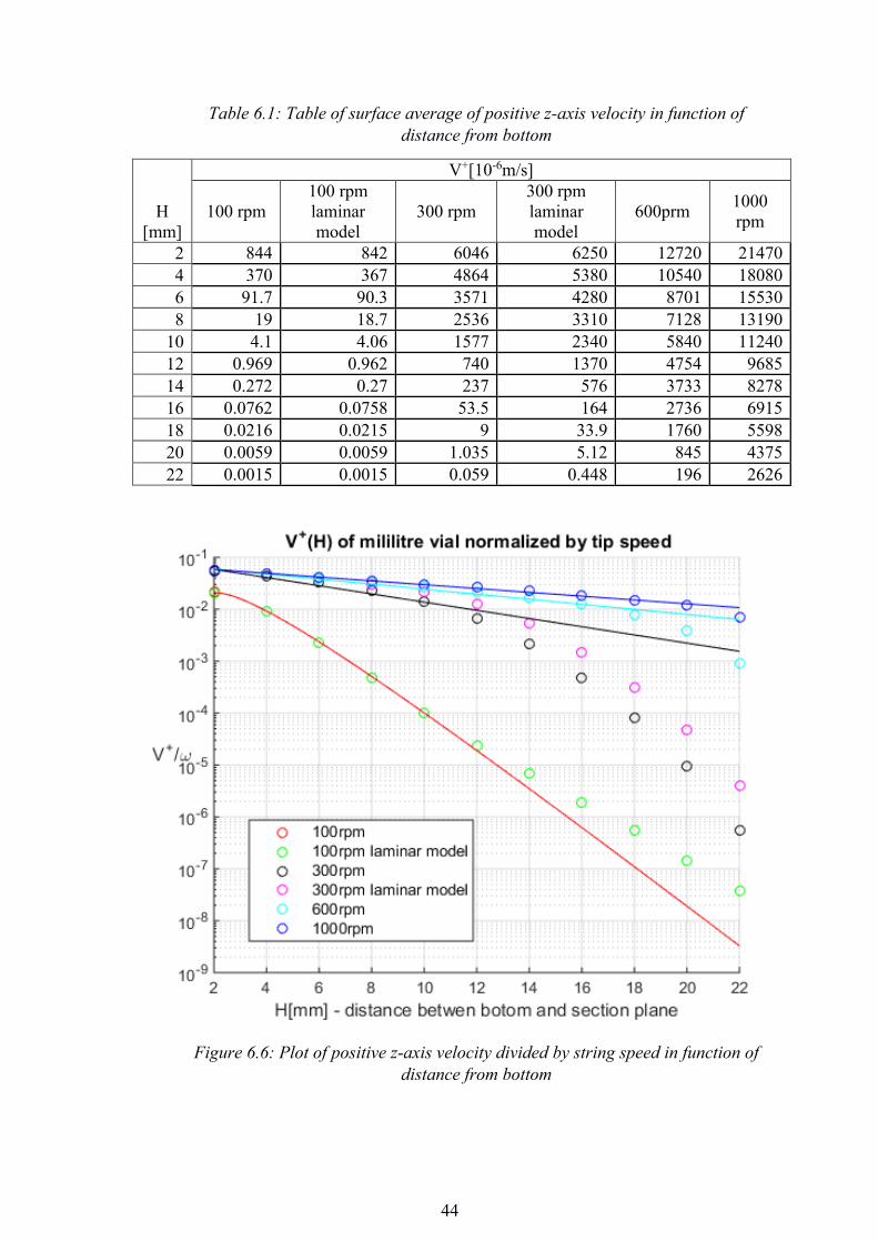
Because data of V+ function from table 7.1 did not show any trend it has been done
normalization by dividing surface average for 11 section planes by linear velocity of end of
magnetic stirrer, data are presented in table 6.2 and also at figure 6.6 and normalization
equation is equation 7.4.
𝑉+𝑛𝑜𝑟𝑚𝑎𝑙𝑖𝑧𝑒𝑑 = ⟨𝑉+⟩
𝜔 6.4
From obtained data it has been observed that for 100 rpm that data shows good level
of convergence up to 10-14 and it can be seen that for this speed of stirring values of V+
function in vial decreases much faster than for 600 and 1000 rpm. It has been also noticed
that for 100 rpm laminar and k-ε models shows consistent results. From these results it has
been obtained that for mostly laminar flow, which is predicted to be at 100 rpms, k-ε model
works fine and give good results.
For 100 rpm it has been noticed that positive z-axis velocity decreases strongly and
exponentially. It is predicted that for 100 rpm flow is laminar and in this case pumping flow
pass by energy slower than for other speed of stirring and because of properties of laminar
flow it has been postulated that mixing it this flow very poorly and probability of secondary
nucleation is predicted to be low.
For 300 rpm it has been observed transition flow that has properties of not developed
turbulent flow and also laminar flow. Until 12mm above bottom it has been observed that
speed gradient is near to turbulent flow and pumping fluid flow speed slow decays but after
reaching 12mm above bottom it start to decrease exponentially and reach laminar gradient
of fluid flow. For laminar and k-ε models it has been observed also deviation between models
which shows that with increasing the rotary speed From that data it has been predicted that

43
secondary nucleation will only occurs in lower parts of the vial and upper parts of vial there
is laminar flow field in which there small possibility of secondary nucleation process.
For 600 and 1000 rpm it has been observed that fluid flow slow decay mode. For 600
rpm it has been observed that flow is turbulent and only after reaching 18mm above bottom
it starts to decrease exponentially. In mostly all of vial volume so shear rate of flow is bigger
than for laminar flow and possibility of secondary nucleation process starts to increase. For
1000 rpm flow in whole vial volume is strictly turbulent and it is observed that pumping
flow ends at surface of liquid.
It has been also noticed that for 300, 600 and 1000 rpm 𝑉+𝑛𝑜𝑟𝑚𝑎𝑙𝑖𝑧𝑒𝑑 at 2mm above
bottom has the same value. It has been observed until 6mm above bottom values of
𝑉+𝑛𝑜𝑟𝑚𝑎𝑙𝑖𝑧𝑒𝑑 are similar to each other and change of it fits to numerical error simulation. It
has been also observed that for turbulent flow field like 600 and 1000 rpm 𝑉+𝑛𝑜𝑟𝑚𝑎𝑙𝑖𝑧𝑒𝑑
shows similar values until even 12mm, where the turbulent flow field in 600 rpm start to
decrease. It has postulated that from obtained data that for more than 1000 rpm flow values
of z-axis normalized velocity will reach the constant values for height above bottom.
Figure 6.5: Plot of surface average of positive z-axis velocity in function of distance from bottom
44
Table 6.1: Table of surface average of positive z-axis velocity in function of distance from bottom
H [mm]
V+[10-6m/s]
100 rpm 100 rpm laminar model
300 rpm 300 rpm laminar model
600prm 1000 rpm
2 844 842 6046 6250 12720 21470 4 370 367 4864 5380 10540 18080 6 91.7 90.3 3571 4280 8701 15530 8 19 18.7 2536 3310 7128 13190
10 4.1 4.06 1577 2340 5840 11240 12 0.969 0.962 740 1370 4754 9685 14 0.272 0.27 237 576 3733 8278 16 0.0762 0.0758 53.5 164 2736 6915 18 0.0216 0.0215 9 33.9 1760 5598 20 0.0059 0.0059 1.035 5.12 845 4375 22 0.0015 0.0015 0.059 0.448 196 2626
Figure 6.6: Plot of positive z-axis velocity divided by string speed in function of distance from bottom
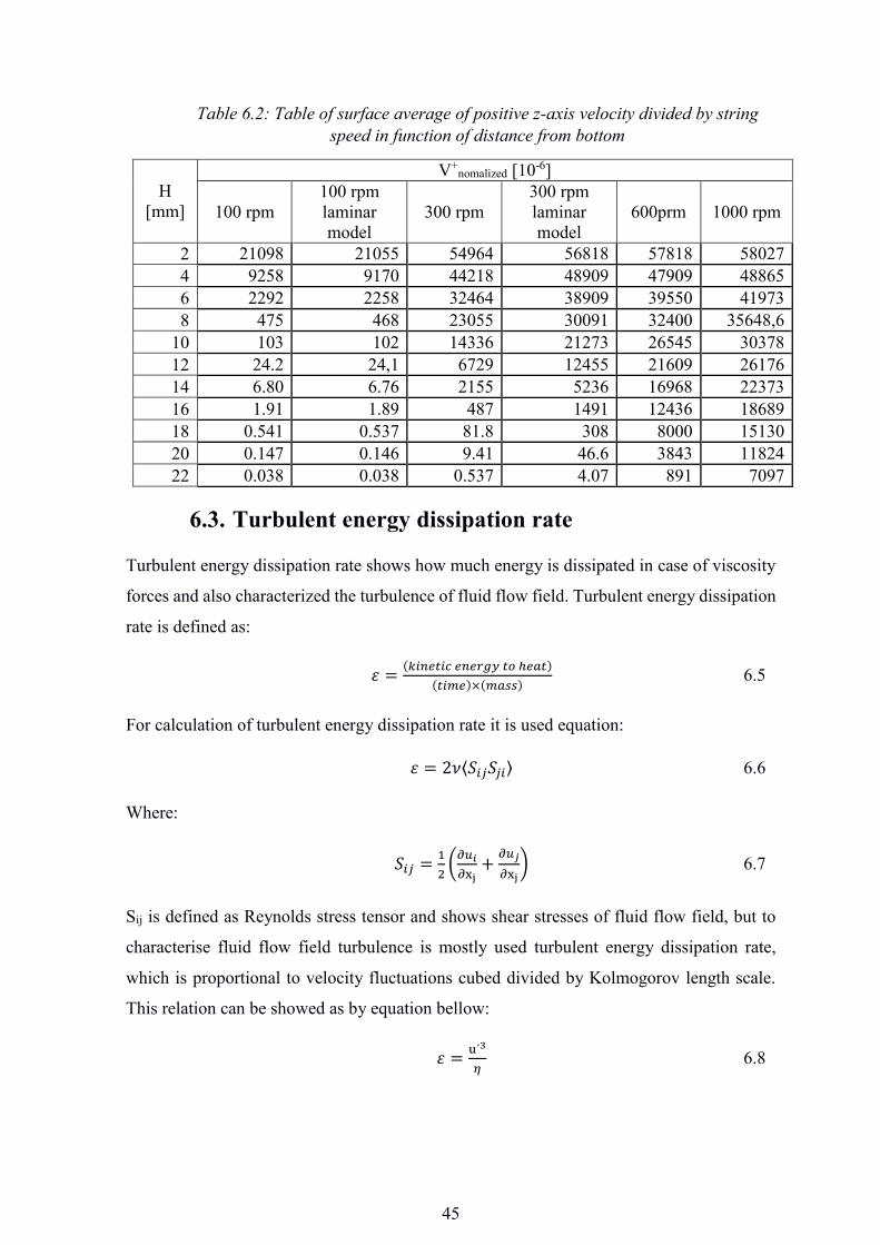
45
Table 6.2: Table of surface average of positive z-axis velocity divided by string speed in function of distance from bottom
H [mm]
V+nomalized [10-6]
100 rpm 100 rpm laminar model
300 rpm 300 rpm laminar model
600prm 1000 rpm
2 21098 21055 54964 56818 57818 58027 4 9258 9170 44218 48909 47909 48865 6 2292 2258 32464 38909 39550 41973 8 475 468 23055 30091 32400 35648,6
10 103 102 14336 21273 26545 30378 12 24.2 24,1 6729 12455 21609 26176 14 6.80 6.76 2155 5236 16968 22373 16 1.91 1.89 487 1491 12436 18689 18 0.541 0.537 81.8 308 8000 15130 20 0.147 0.146 9.41 46.6 3843 11824 22 0.038 0.038 0.537 4.07 891 7097
6.3. Turbulent energy dissipation rate
Turbulent energy dissipation rate shows how much energy is dissipated in case of viscosity
forces and also characterized the turbulence of fluid flow field. Turbulent energy dissipation
rate is defined as:
𝜀 = (𝑘𝑖𝑛𝑒𝑡𝑖𝑐𝑒𝑛𝑒𝑟𝑔𝑦𝑡𝑜ℎ𝑒𝑎𝑡)(𝑡𝑖𝑚𝑒)×(𝑚𝑎𝑠𝑠)
6.5
For calculation of turbulent energy dissipation rate it is used equation:
𝜀 = 2𝜈⟨𝑆𝑖𝑗𝑆𝑗𝑖⟩ 6.6
Where:
𝑆𝑖𝑗 = 12(∂𝑢𝑖
∂xj+ ∂𝑢𝑗
∂xj) 6.7
Sij is defined as Reynolds stress tensor and shows shear stresses of fluid flow field, but to
characterise fluid flow field turbulence is mostly used turbulent energy dissipation rate,
which is proportional to velocity fluctuations cubed divided by Kolmogorov length scale.
This relation can be showed as by equation bellow:
𝜀 = u´3
𝜂 6.8

46
Where:
u´- velocity fluctuations [m/s]
η- Kolmogorov length scale [m]
Kolmogorov length scale characterise the smallest dimension of turbulences that will not be
dissipated in to internal energy. It has been definite by Kolmogorov in 1941[Kolmogorov
1941] and is comes out from dimension analyse. In 1941 it has been proposed as one of third
microscales. Kolmogorov length scale is definite as:
𝜂 = (𝜐3
𝜀)
14 6.9
Velocity fluctuations are defined as a module from difference between actual value of fluid
flow velocity and average fluid flow velocity. Velocity fluctuations tell about local
turbulences and allow to calculate turbulent intensity. By calculating turbulence intensity it
possible to observe if flow is turbulent or laminar and predict fluid flow properties better
than using Reynolds criteria number.
From turbulent energy dissipation rate has been made a volume average which is defined as:
⟨𝜀⟩ = 1𝑉 ∮ 𝜀 𝑑𝑉
𝑉 6.10
Where:
V- Volume of the system
dV- Volume element.
Results for turbulent energy dissipation rate are listed out at table 6.3 and plotted at figure
6.7. From turbulent kinetic energy has been made a volume average in the same way as for
turbulent energy dissipation rate and listed out at table 6.3 and plotted at figure 6.8. It has
been clearly seen that turbulent energy dissipation rate and turbulent kinetic energy grows
in power law with increasing the speed of stirring.
To understand this phenomena it has been recalled the equation for calculation average of
turbulent energy dissipation rate where velocity fluctuation are proportional in square way
to velocity fluctuations and defined Γ the characteristic velocity gradient which is
proportional to rotary speed of the impeller which is expected behaviour of laminar flow.

47
The scally for k is expected to consider that utip is proportional to rotary speed, therefore u`
is proportional to utip and Γ½.
From turbulent energy dissipation rate it has been calculated the dissipated power by using
equation:
𝑃𝑚 = ⟨𝜀⟩𝑉𝜌 6.11
Where:
⟨𝜀⟩-Volume average of turbulent energy dissipation rate [m2/ s3]
V-Volume of system [m3]
ρ- Density of fluid [kg/m3]
Volume of vial is estimated as a cylinder with dimensions shown at figure 4.1, and it is
calculated as:
𝑉 = 𝐷2𝐻𝜋4
6.12
Where:
D=10[mm]- inside diameter of the vial.
H=23.4[mm]-inside height of the vial.
𝑉 =(10𝑚𝑚)2𝜋
4∙ (23.4𝑚𝑚) = 1.84 ∙ 10−6[𝑚3]
It has been assumed that Water is in standard conditions so density of water is
ρ=998.2071[kg/m3] (Weast, 1989) and constant-pressure heat capacity in 1atm is
Cp=4.1818[J/g K] (Weast, 1989). .Dissipated power has been listed in table 6.3.
To better investigate the fluid flow properties it has been done calculations of power number
which is ration between resistance force and inertia force. Power number is defined as:
𝑃𝑁 = 𝑃𝑚𝜌𝑁3𝐷5 6.13
Where:
N- Rotational speed [1/s]

48
For power number it has been made calculations for rotations speed from 100 to 1000 rpm
and listed out at table 6.3 and plotted at figure 6.9. Power number plots shows if flow is
turbulent or laminar. In case of turbulent flow power number starts to become nearly
constant, but for laminar flow it still decrease until it reach the constant low value and flow
become turbulent.
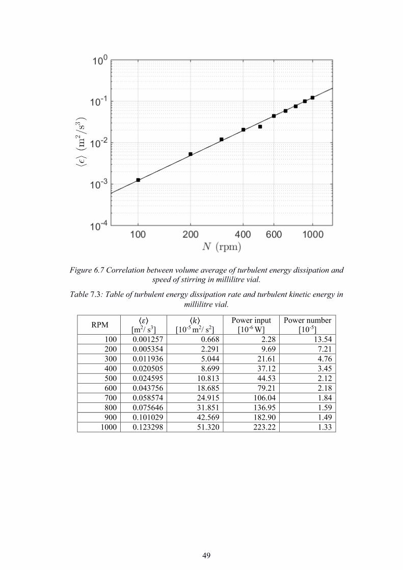
The scaling for <ε> is in unexpected. Typically for a turbulent stirred tank it has been find
out that⟨𝜀⟩~𝑁3. This cubic scaling follows directly from a Power number. Power number is
reads as𝑃𝑁~ 𝜀𝑁3⁄ , if epsilon goes up the power number reach constant value and epsilon
became proportional to speed of stirring.
Therefore, the scaling of <ε> which is seen in figure 6.7 implication that the dissipation of
energy is controlled by mainly by flow in boundary layer. This means that flow has mostly
laminar properties but is should be also noticed from other fluid flow properties that for
speed of stirring above 600 rpm positive z-axis velocity plots shows that flow has also
turbulent properties. This goes to conclusion that flow in millilitre vial above 600 rpm is
predicted to be transient because it has properties of laminar and turbulent flow in the same
time. It should be also noticed that properties of the system, especially the turbulence of flow
field should be investigated also experimentally to observe if fluid flow shows turbulent or
laminar properties.
From plot at figure 6.9 it is clearly seen that power number decreases with a speed of stirring
in power of 10-1.04. From that correlation it can be easily seen that flow is laminar but for
higher speed, more than 800 rpm of stirring it is visible that power number stars to slow
down decreasing and it is predicted that for more than 1000 rpm flow can become turbulent.
49
Figure 6.7 Correlation between volume average of turbulent energy dissipation and
speed of stirring in millilitre vial.
Table 7.3: Table of turbulent energy dissipation rate and turbulent kinetic energy in millilitre vial.
RPM ⟨𝜀⟩ [m2/ s3]
⟨𝑘⟩ [10-5 m2/ s2]
Power input [10-6 W]
Power number [10-5]
100 0.001257 0.668 2.28 13.54 200 0.005354 2.291 9.69 7.21 300 0.011936 5.044 21.61 4.76 400 0.020505 8.699 37.12 3.45 500 0.024595 10.813 44.53 2.12 600 0.043756 18.685 79.21 2.18 700 0.058574 24.915 106.04 1.84 800 0.075646 31.851 136.95 1.59 900 0.101029 42.569 182.90 1.49
1000 0.123298 51.320 223.22 1.33

50
Figure 6.8. Correlation between volume average of kinetic energy and speed of stirring
in millilitre vial.
Figure 6.9. Correlation between power number and speed of stirring in millilitre vial.

51
6.4. Checking influence of stirring to temperature change
in the model.
In this work it has not been simulated the temperature change but is has been assumed
that temperature change is not important for fluid flow properties. It has been also assumed
that walls of system are adiabatic. Vial is fully filed by fluid and volume of stirrer is
negligible.
To calculate temperature change per second has been made simple thermodynamic
balance:
𝑃𝑚 = 𝑉∆�̇�𝐶𝑝𝜌 6.14
Where:
∆�̇�- Temperature change per second [K/s]
According to previous equations:
𝑉∆�̇�𝐶𝑝𝜌 = ⟨𝜀⟩𝑉𝜌 6.15
∆�̇� = ⟨𝜀⟩𝐶𝑝
6.16
Temperature change per second has been listed in table 6.4. From obtained data it
has been assumed that temperature change is not bigger than 0.0003 [K/s] that confirm the
assuming about constant temperature of fluid flow is correct, because this amount of
generated power is at up to range of 10-3 W, will be easy dissipated in environment by walls
of system.
It is clearly seen according to made calculations that temperature is independent from
dissipating energy in mixing process.
It should be also noticed that to make 1K temperatures change in a millilitre vial for
100 rpm it would take approximately 93hours which is around 4days but for 1000 rpm it
should be noticed that it would take approximately an hour, which shows that above a 1000
rpms it should be consider temperature change in the vial because of energy dissipation in
fluid.

52
Table 6.4: Table of power input and temperature change per second in millilitre vial.
RPM Power input
[10-6 W]
Temperature
change
[10-5 K/s]
Time to change
temperature for
1K
[s]
Time to change
temperature for
1K
[h]
100 2,28 0,30 333333 92,59
200 9,69 1,28 78125 21,70
300 21,61 2,85 35088 9,75
400 37,12 4,90 20408 5,67
500 44,53 5,88 17007 4,72
600 79,21 10,46 9560 2,66
700 106,04 14,01 7138 1,98
800 136,95 18,09 5528 1,54
900 182,90 24,16 4139 1,15
1000 223,22 29,48 3392 0,94

53
Conclusions From obtained data from CFD simulation and calculations made according to CFD
simulation data it has been clearly seen that fluid flow filed did not reach the fully turbulent
flow and only become transient for stirring speed faster than 500 rpm. It has been also
noticed that Reynolds criteria for this fluid flow field should be investigated in future work
to develop criteria for bolder between laminar and transient fluid flow filed.
It is worth to notice that k-ε model was also suitable to strictly laminar flow fields
and turbulence modelling was becoming important for stirring speed even from 300 rpm
where fluid flow was predicted to be laminar. From obtained data has been also visible that
difference in results between laminar and k-ε model is not significant and results are
comparative to each other for low rotary speeds, but with increasing the rotary speed results
become less similar to each other. This phenomena is can be explained as influence of
turbulent modelling to calculation results. In laminar model there is no turbulence modelling
which support calculations of local eddies in k-ε model.
It has been also noticed from positive z-axis velocity surface average plot that for
with increasing the speed of stirring influence of used model for calculation results become
more visible and for 100 rpm there is no influence of the model for calculations but for rotary
speed more than 300 rpm differences between models with confirm results from contour
plots.
Used boundary conditions do not have a big influence on results of fluid flow field
for all simulated rotary speeds. It should be also noticed that assumption about constant
temperature and simulation upper surface as a wall boundary condition were correct. From
calculation based on time CFD simulation results assumption of constant temperature has
been validated and as it has been check for millilitre vial in adiabatic conditions. Results of
calculations shows that only for 1000 rpm temperature change influence should be
considered in long experiments, which take more than 1 hour and there are made in adiabatic
conditions. In real lab scale experiments millilitre vials are always in water or air
environment and mostly of cases temperature is strictly monitored and regulated by
thermostatic devices, so assumptions were correct. For experiments with a temperature
which change, are made for crystallization, is strongly recommended to develop correction
factors for fluid flow fields based on lab scale experiments.
54
From experiments has been noticed that for 1000 rpm effect of mass and Coriolis
forces on upper surface of liquid are nearable and modulating free surface of liquid as a wall
provide a good simulation results and speed up calculations with no big negative impact on
possible effect from free upper surface of liquid. It has been also observed that more impact
on shape of free surface has surface tension and capillary forces than stirring.
From acquired contour plots it clearly visible that until reaching 600 rpm area of first
velocity flow field area is increasing proportional to rotary speed but after reaching 600 rpm
area of first velocity field become constant increasing the area of velocity gradient is based
on increasing firstly second and then third velocity filed area.
From vector plots of velocity field it has been visible that main up pumping flow
goes near to walls and fluid flow circulations patterns are becoming from nearly circles to
fully elliptical with increasing the stirring speed in millilitre vial. This behaviour was
expected from theoretical predictions and confirm that fluid flow fields’ simulation results
are correct. It should be also noticed that for more than 600 rpm flow laminar layer near to
walls and bottom become smaller and mixing is provided by stirrer not only up to the stirrer
but also near to the bottom of the vial.
From positive z-axis velocity surface average plot has been observed that with
increasing stirring speed fluid flow field starts to pass energy using turbulent viscosity in
more linear way with increasing the height of the vial. It has been also observed that for
strictly laminar fluid flow fields, which occurs from 100 to 300 rpm velocity gradient
decrease more in logarithmic way and after normalization it has been observed that all
velocity flow fields has the same value of start point for transient flow. It has been realized
that almost zero velocity point z-axis coordinate goes linear up with increasing the stirring
speed.
From obtained data it has to been assumed that there is no strict criteria for fluid flow
fields in millilitre vial to predict if flow field will be turbulent or laminar and this can be
only discovered using lab experiments. It has been also realized that using Reynolds number
to predict fluid flow field properties is useless because from Reynold number all fluid flow
fields should be laminar but from obtained properties it is clearly seen that fluid flow field
starts to show transient fluid flow properties from 400 rpm, and for 100 rpm fluid flow field
is turbulent.

55
References
Allonneau, Charline, Eric Olmos, Stéphane Guyot, Eric Ferret, Patrick Gervais, and Rémy Cachon. 2015. "Hydrodynamic Characterization Of A New Small-Scale Reactor Mixed By A Magnetic Bar". Biochemical Engineering Journal 96: 29-37. doi:10.1016/j.bej.2014.12.005.
Bai, Ge, Jared S. Bee, James G. Biddlecombe, Quanmin Chen, and W. Thomas Leach. 2012. "Computational Fluid Dynamics (CFD) Insights Into Agitation Stress Methods In Biopharmaceutical Development". International Journal Of Pharmaceutics 423 (2): 264-280. doi:10.1016/j.ijpharm.2011.11.044.
Dubrovskiı̆, V. G. 2005. "Growth Kinetics Of Thin Films Formed By Nucleation During Layer Formation". Semiconductors 39 (11): 1267. doi:10.1134/1.2128448.
Forsyth, Carol, Iain S. Burns, Paul A. Mulheran, and Jan Sefcik. 2016. "Scaling Of Glycine Nucleation Kinetics With Shear Rate And Glass–Liquid Interfacial Area". Crystal Growth & Design 16 (1): 136-144. doi:10.1021/acs.cgd.5b01042.
Forsyth, Carol, Paul A. Mulheran, Claire Forsyth, Mark D. Haw, Iain S. Burns, and Jan Sefcik. 2015. "Influence Of Controlled Fluid Shear On Nucleation Rates In Glycine Aqueous Solutions". Crystal Growth & Design 15 (1): 94-102. doi:10.1021/cg5008878.
Granberg, Roger A. and Åke C. Rasmuson. 1999. "Solubility Of Paracetamol In Pure Solvents". Journal Of Chemical & Engineering Data 44 (6): 1391-1395. doi:10.1021/je990124v.
Hortsch, Ralf and Dirk Weuster-Botz. 2009. "Power Consumption And Maximum Energy Dissipation In A Milliliter-Scale Bioreactor". Biotechnol Progress, NA-NA. doi:10.1002/btpr.338.
Jiang, Shanfeng and Joop H. ter Horst. 2011. "Crystal Nucleation Rates From Probability Distributions Of Induction Times". Crystal Growth & Design 11 (1): 256-261. doi:10.1021/cg101213q.
Kadam, Somnath S., Herman J. M. Kramer, and Joop H. ter Horst. 2011. "Combination Of A Single Primary Nucleation Event And Secondary Nucleation In Crystallization Processes". Crystal Growth & Design 11 (4): 1271-1277. doi:10.1021/cg101504c.
Liu, Jin and Åke C. Rasmuson. 2013. "Influence Of Agitation And Fluid Shear On Primary Nucleation In Solution". Crystal Growth & Design 13 (10): 4385-4394. doi:10.1021/cg4007636.
Liu, Jin, Michael Svärd, and Åke C. Rasmuson. 2015. "Influence Of Agitation On Primary Nucleation In Stirred Tank Crystallizers". Crystal Growth & Design 15 (9): 4177-4184. doi:10.1021/cg501791q.
Mullin, J. W. 2001. Crystallization. Oxford: Butterworth-Heinemann.

56
Myerson, Allan S. 2002. Handbook Of Industrial Crystallization. Boston: Butterworth-Heinemann.
"Operating Parameters - Crystallization Systems". 2016. Crystallizationsystems.Com. https://www.crystallizationsystems.com/crystal16/operating-parameters-crystal16, 2016-06-22.
Pope, S. B. 2000. Turbulent Flows. Cambridge: Cambridge University Press.
Weast, Robert C. 1989. CRC Handbook Of Chemistry And Physics. Boca Raton, FL: CRC Press.
Wendt, John F and John D Anderson. 2009. Computational Fluid Dynamics. Berlin: Springer.
Wikipedia,. 2016. Image. https://upload.wikimedia.org/wikipedia/commons/e/ee/Plot_of_classical_nucleation_theory_prediction_for_the_free_energy_of_a_nucleus_as_a_function_of_radius.png.


58
Marcin Janusz Kołakowski
234916
IPP ICHIP
Warszawa, 26 lipca 2016