Center for Computational Engineering ScienceMathematics DivisionHead of Institute: Prof. Dr. Manuel Torrilhon

Bachelor Thesis

CFD Simulation of Internal Arc Faults in Gas-Insolated

High-Voltage Switchgear

Lukas Bischoff

Scientific Supervisors

Prof. Dr. Manuel Torrilhon

Dr. Jorg Ostrowski

Faculty for Mechanical Engineering

RWTH Aachen University

August 2014

I hereby declare that I have written this bachelor thesis completely on

my own. The external sources, data, and support that I have used are

clearly mentioned and have marked citations accordingly.

Zurich, August 2014

Lukas Bischoff

Contents

List of Figures vii

List of Tables ix

Glossary xi

1 Introduction 1

2 Internal Arcs in High-Voltage Gas-Insulated Switchgear 32.1 Gas Insulated Switchgear . . . . . . . . . . . . . . . . . . . . 32.2 Internal Arc Faults . . . . . . . . . . . . . . . . . . . . . . . . 4

2.3 Burst Disk . . . . . . . . . . . . . . . . . . . . . . . . . . . . . 62.4 Sulfur Hexafluoride . . . . . . . . . . . . . . . . . . . . . . . 6

3 Physics of Internal Arcs 93.1 Internal Arcs . . . . . . . . . . . . . . . . . . . . . . . . . . . 9

3.2 Heat Transfer . . . . . . . . . . . . . . . . . . . . . . . . . . . 93.3 Electrode Erosion . . . . . . . . . . . . . . . . . . . . . . . . 123.4 Chemical Reactions . . . . . . . . . . . . . . . . . . . . . . . 13

4 Modeling 174.1 Physical Modeling . . . . . . . . . . . . . . . . . . . . . . . . 17

4.1.1 Arc Model . . . . . . . . . . . . . . . . . . . . . . . . 174.1.2 Gas Model . . . . . . . . . . . . . . . . . . . . . . . . 21

4.1.3 Radiation Model . . . . . . . . . . . . . . . . . . . . . 224.1.4 Erosion Model . . . . . . . . . . . . . . . . . . . . . . 234.1.5 Arc Movement . . . . . . . . . . . . . . . . . . . . . . 24

4.2 Numerical Modeling . . . . . . . . . . . . . . . . . . . . . . . 254.2.1 Computational Fluid Dynamics . . . . . . . . . . . . 254.2.2 Flow Numerics . . . . . . . . . . . . . . . . . . . . . . 25

4.2.3 Gas Numerics . . . . . . . . . . . . . . . . . . . . . . 264.2.4 Radiation Model . . . . . . . . . . . . . . . . . . . . . 27

4.3 Meshing and Case Setup . . . . . . . . . . . . . . . . . . . . 27

4.3.1 Meshing . . . . . . . . . . . . . . . . . . . . . . . . . . 27

vi Contents

4.3.2 Boundary Conditions . . . . . . . . . . . . . . . . . . 294.3.3 Simulation Input . . . . . . . . . . . . . . . . . . . . 30

5 Results and Analysis 335.1 2D vs 3D Pressure Surge . . . . . . . . . . . . . . . . . . . . 335.2 2D vs 3D Outflow Function . . . . . . . . . . . . . . . . . . 355.3 Burst Disk Modification . . . . . . . . . . . . . . . . . . . . . 395.4 Influence of the Arc Position . . . . . . . . . . . . . . . . . . 41

6 Conclusion 43

Bibliography I

A Appendix IIIA.1 Burst Disk Script . . . . . . . . . . . . . . . . . . . . . . . . . IIIA.2 Power and Mass Input Script . . . . . . . . . . . . . . . . . VA.3 Spacial Diagrams, 2D vs 3D Pressure Surge Investigation IX

List of Figures

2.1 550kV ABB Bus Bars . . . . . . . . . . . . . . . . . . . . . . 32.2 300kV ABB Bus Bars . . . . . . . . . . . . . . . . . . . . . . 32.3 Internal Arc Fault Inside a Bus Bar . . . . . . . . . . . . . . 4

3.1 Radiation Transport . . . . . . . . . . . . . . . . . . . . . . . 103.2 SF6 Absorption Coefficient Over Radiation Frequency for

1MPa; Red Line Marks the Chosen Absorption Coefficientfor this Work . . . . . . . . . . . . . . . . . . . . . . . . . . . 11

3.3 Vaporization at the Arc Roots . . . . . . . . . . . . . . . . . 123.4 SF6 Density Over Temperature for 1MPa . . . . . . . . . . 14

4.1 Effects of an Internal Arc Fault . . . . . . . . . . . . . . . . 17

4.2 Arc Volume Model . . . . . . . . . . . . . . . . . . . . . . . . 194.3 Geometry Including Boundary Conditions . . . . . . . . . . 284.4 Volumetric Energy and Mass Input Rates, RMS Values in

Bold . . . . . . . . . . . . . . . . . . . . . . . . . . . . . . . . 31

5.1 Sensor Positions, 2D vs 3D Pressure Surge Investigation . 335.2 Temperature and Density Diagram, 2D vs 3D Pressure

Surge Investigation . . . . . . . . . . . . . . . . . . . . . . . . 345.3 Pressure Diagram, 2D vs 3D Pressure Surge Investigation 355.4 Pressure Diagram, 2D vs 3D Outflow Investigation . . . . 365.5 Mass and Energy Flow Diagrams, 2D vs 3D Outflow In-

vestigation . . . . . . . . . . . . . . . . . . . . . . . . . . . . . 375.6 Temperature Profiles in Kelvin, Burst Disk Marked in Red,

2D vs 3D Outflow Investigation . . . . . . . . . . . . . . . . 375.7 Pressure Diagram, 3m × 0.15m Geometry, 2D vs 3D Out-

flow Investigation . . . . . . . . . . . . . . . . . . . . . . . . . 385.8 Pressure Diagram, 2D vs 3D Outflow Modification . . . . . 405.9 Mach Number at 0.13s, 2D vs 3D Outflow Modification . . 405.10 2D Pressure Diagram, Burst Disk Opening Times are Slightly

Different for All Cases, Arc Position Investigation . . . . . 415.11 3D Pressure Diagram, Burst Disk Opening Times are Slightly

Different for All Cases, Arc Position Investigation . . . . . 42

viii List of Figures

A.1 Spacial Mass Fraction Al, 2D vs 3D Pressure Surge Inves-tigation . . . . . . . . . . . . . . . . . . . . . . . . . . . . . . . IX

A.2 Spacial Axial Velocity, 2D vs 3D Pressure Surge Investigation IXA.3 Spacial Density, 2D vs 3D Pressure Surge Investigation . . XA.4 Spacial Incident Radiation, 2D vs 3D Pressure Surge In-

vestigation . . . . . . . . . . . . . . . . . . . . . . . . . . . . . XA.5 Spacial Pressure, 2D vs 3D Pressure Surge Investigation . XIA.6 Spacial Temperature, 2D vs 3D Pressure Surge Investigation XI

List of Tables

2.1 Properties of SF6 and Air at 20○C and 0.1MPa . . . . . . . 6

5.1 Arc Model Setup, 2D vs 3D Pressure Surge Investigation . 335.2 Pressure Peaks, Arc Position Investigation . . . . . . . . . . 41

Glossary

Abbreviations

Al AluminumCB Circuit BreakerCFD Computational Fluid DynamicsCIGRE Conseil international des grands reseaux

electriques / International Council on LargeElectric Systems

CO2 Carbon DioxideFVM Finite Volume MethodGIS Gas Isolated SwitchgearIEC International Electrotechnical CommissionMHD MagnetohydrodynamicsRMS Root Mean SquareSF6 Sulfur Hexafluoride

Greek letters

α absorption coefficient [m−1]αs scattering coefficient [m−1]ρ density [kgm−3]σ Stefan-Boltzmann constant [kgs−3K−4]τ stress tensor [kgm−1s−2]

Roman letters

A area [m2]C phase function coefficient [−]cvap vaporization constant [kgA−1s−1]E energy [kgm2s−2]F external forces [kgms−2]

xii Glossary

G incident radiation [kgs−3]g gravitational force [kgms−2]∆H enthalpy [kgm2s−2]I radiation intensity [kgm2s−2]Iarc arc current [A]J diffusion flux [kgm−2s−1]kp pressure transfer coefficient [−]mvap evaporation mass rate [kgs−1]p pressure [kgm−1s−2]qr radiation flux [kgs−3]Ri rate of production of species i from electrode

erosion[kgs−1]

Sh energy source term [kg2m−1s−3]Sm mass source term [kgm−3s−1]t time [s]P power [kgm2s−3]T temperature [K]U internal energy [kgm2s−2]Uarc arc voltage [kgm2s−3A−1]∆Ueff effective voltage drop [kgm2s−3A−1]v velocity [ms−1]We electric input energy [kgm2s−2]Yi mass fraction of species i [−]

1 Introduction

The pressure rise due to internal arc faults in large, gas insulated switchgear

(GIS) can cause great damage and be very dangerous to humans. Man-

ufacturers of high-voltage switchgear such as ABB are therefore trying

to minimize the risk of internal arc faults through constructive measures.

Nevertheless, the risk cannot be eliminated completely which means that

switchgear has to be dimensioned to withstand the forces and tempera-

tures caused by internal arc faults. A commonly used safety mechanism

is the installation of burst disks at critical points in the device to ensure a

controlled pressure release and prevent dangerous explosions and pressure

damage. The pressure build up and distribution inside the GIS’s insula-

tion chamber must be investigated in order to determine the best location

for the burst disk, the appropriate size, and the pressure it should trigger

at.

Besides experiments, simulations have become a major field of research

to construct high-voltage switchgear that is safe in the event of an internal

arc fault. The IEC Norm 62271-203 allows the use of simulations as an

alternative to experiments for the certification of high-voltage switchgear.

Simulations are particularly advantageous in this field of research, as the

required safety precautions are very costly in high-voltage switchgear ex-

periments. Due to the release of a considerable amount of Sulfur Hex-

afluoride (SF6) into the atmosphere these experiments are also extremely

harmful to the environment.

In the course of this work a model to simulate the pressure build up

as well as the pressure release through a burst disk inside the bus bar

section of a GIS was developed and implemented. The main focus was

on the investigation of differences in results when using 2D axisymmetric

2 1 Introduction

meshes instead of 3D meshes. This is of enormous interest as 2D meshes

are simpler to create and can be simulated with less computational effort.

Another focus was on the influence the arc position has on the pressure

build up and especially the pressure peak inside the GIS in the event of an

arc fault. This was necessary to determine whether the simulation model

needs to extended through the implementation of arc movement.

2 Internal Arcs in High-VoltageGas-Insulated Switchgear

2.1 Gas Insulated Switchgear

Figure 2.1: 550kV ABB Bus Bars

Switchgear is a type of machinery

used in electrical power systems. It

can consist of switches, fuses and

circuit breakers connected through

bus bars and used to control, iso-

late and protect electric equipment.

Switchgear is an essential part of

every modern power grid. It is

used to disconnect and de-energize

power lines in the event of a fault

or for maintenance reasons. Among the largest worldwide manufacturers

of switchgear are ABB, Alstom, General Electric and Siemens.

Figure 2.2: 300kV ABB Bus Bars

Modern switchgear is commonly

classified by its insulation mate-

rial. The simplest constructions

use air based insulation. However,

at high voltages this is extremely

space consuming due to the space

needed around energized parts to

prevent electric arcs. More effec-

tive insulating media are gases (es-

pecially SF6), oil or vacuum. Presently, gas insulated switchgear is com-

4 2 Internal Arcs in High-Voltage Gas-Insulated Switchgear

monly used in the high (>75kV) and ultra high (>250kV) voltage range

with the highest licensed voltage being 1200kV. GIS reduces the space

requirements to around 15% of comparable air insulated switchgear and

is safe for human contact through its casing.

2.2 Internal Arc Faults

Bus bars are simple power lines connecting the different parts of the

switchgear. Due to their close proximity to other parts of the switchgear

they are surrounded by an enclosure with the insulating media (in this

work SF6) filling up the space between internal conductor and enclosure.

This way electric arcs between different parts of the switchgear are pre-

vented and humans cannot come in contact with the current carrying

internal conductor. In the event of an internal arc fault, an electric arc

forms between the internal conductor and the enclosure as shown in Fig-

ure 2.3.

Enclosure

Internal Conductor

Arc Fault

SF6

Figure 2.3: Internal Arc Fault Inside a Bus Bar

This can be the result of a surge in the power grid, faulty insulation or

human error. Studies on the frequency of internal arc faults carried out by

the CIRGE show that the average error frequency when running a circuit

2.2 Internal Arc Faults 5

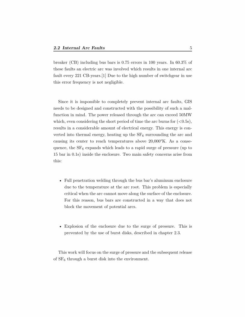
breaker (CB) including bus bars is 0.75 errors in 100 years. In 60.3% of

these faults an electric arc was involved which results in one internal arc

fault every 221 CB-years.[1] Due to the high number of switchgear in use

this error frequency is not negligible.

Since it is impossible to completely prevent internal arc faults, GIS

needs to be designed and constructed with the possibility of such a mal-

function in mind. The power released through the arc can exceed 50MW

which, even considering the short period of time the arc burns for (<0.5s),

results in a considerable amount of electrical energy. This energy is con-

verted into thermal energy, heating up the SF6 surrounding the arc and

causing its center to reach temperatures above 20,000°K. As a conse-

quence, the SF6 expands which leads to a rapid surge of pressure (up to

15 bar in 0.1s) inside the enclosure. Two main safety concerns arise from

this:

• Full penetration welding through the bus bar’s aluminum enclosure

due to the temperature at the arc root. This problem is especially

critical when the arc cannot move along the surface of the enclosure.

For this reason, bus bars are constructed in a way that does not

block the movement of potential arcs.

• Explosion of the enclosure due to the surge of pressure. This is

prevented by the use of burst disks, described in chapter 2.3.

This work will focus on the surge of pressure and the subsequent release

of SF6 through a burst disk into the environment.

6 2 Internal Arcs in High-Voltage Gas-Insulated Switchgear

2.3 Burst Disk

The aforementioned rapid surge of pressure and the potential explosion of

the casing can be very dangerous to people operating the switchgear. It is

circumvented by including burst disks into the casing. These disks, manu-

factured e.g. from nickel-chromium alloys, copper alloys or steel, rupture

at a predefined pressure difference between their two sides.[2] This guar-

antees a much more controlled release of SF6 into the environment that

takes place at a dedicated position. Furthermore, it is extremely reliable

as it is a purely mechanical process that does not rely on sensors and

other potentially error-prone electronics. Burst disks are therefore one of

the most common safety mechanisms in high pressure applications.

2.4 Sulfur Hexafluoride

SF6 is an inorganic, colorless, odorless, non-flammable, extremely potent

greenhouse gas. Over the past 50 years it was used in various applications

such as electric insulation in medical and electrical equipment, acoustic

insulation in double glazed windows, a tracer in airflow and leakage anal-

ysis and to provide a special atmosphere for metallurgical processes in

military applications.[3]

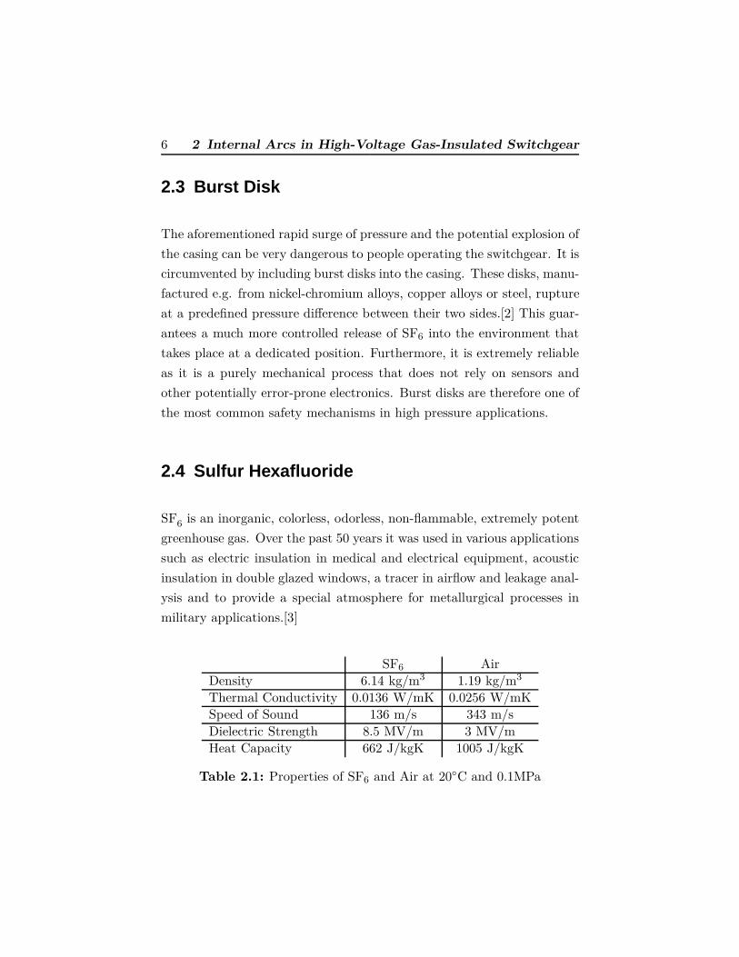
SF6 Air

Density 6.14 kg/m3 1.19 kg/m3

Thermal Conductivity 0.0136 W/mK 0.0256 W/mK

Speed of Sound 136 m/s 343 m/s

Dielectric Strength 8.5 MV/m 3 MV/m

Heat Capacity 662 J/kgK 1005 J/kgK

Table 2.1: Properties of SF6 and Air at 20○C and 0.1MPa

2.4 Sulfur Hexafluoride 7

SF6 is popular as an electric insulator in high-voltage switchgear be-

cause of its dielectric strength that is 2.5 times higher than that of air.

Furthermore, its self-healing behavior causes it to re-form quickly after

being ionized by an arc. As a consequence, modern medium and high-

voltage GIS is almost exclusively operated with SF6 as insulating medium.

Because of its climate-damaging character, it is one of six greenhouse

gases that are part of the Kyoto Protocol of 1997.[4] The usage of SF6 in

Europe is regulated by the F-Gas directive which bans its usage with the

exception of certain applications such as high-voltage switchgear. Studies

suggest that SF6 is the most potent greenhouse gas with a global warming

potential around 23,900 times higher than that of CO2.[3]

For this reason, manufactures of GIS try to reduce their usage of SF6

as far as possible. Completely eliminating SF6 in the ultra high-voltage

segment is not possible, but by adding Nitrogen it is possible to reduce the

amount of SF6 used without significantly sacrificing its insulating proper-

ties. Replacing SF6 with CO2 as the arc-extinguishing medium, ABB was

able to produce a 75kV circuit breaker that, compared to a similar sized

SF6 product, reduces emissions by the equivalent of 10 tons of CO2 dur-

ing its life-cycle. Since experiments involving SF6 insulated switchgear

cause the release of considerable amounts of SF6 into the environment

simulations offer companies such as ABB an ecofriendly alternative.

3 Physics of Internal Arcs

3.1 Internal Arcs

Internal arc faults in bus bar’s occur when the voltage between the enclo-

sure and the internal conductor is high enough to breach the dielectrically

weakest point between them. Local weaknesses can be a consequence of

improper installation, moisture, whiskers or other contaminations. Due

to the arc’s extreme temperatures, the insulating gas forms a highly-

conductive plasma that sustains the current and conducts as much en-

ergy as is available. Its only limitation is the impedance of the arc itself

and the overall system. The arc’s heat vaporizes the electrode material,

discussed in more detail in section 3.3. This causes an explosive volu-

metric increase which in the case of copper is around 64,000 from solid

to vapor.[5] Furthermore, the SF6 is dissociated as a consequence of the

high temperatures which is discussed in more detail in section 3.4.

3.2 Heat Transfer

The extreme temperatures of the arc make the simulation of heat transfer

a key part of the model. The following forms of heat transfer are included

into the model, listed in the order of influence.

• Convection

• Radiation

• Conduction

10 3 Physics of Internal Arcs

While the burst disk is closed, convection occurs as the hot gas inside

the air expands away from it. When the burst disk opens the heated

SF6 is released, making convection by far the biggest contributer to the

cooling of the domain.

The power emitted by radiation scales with the fourth power of the

temperature as evident from the Stefan-Boltzmann law:

P = σ ⋅A ⋅ T 4

with σ being the Stefan-Boltzmann constant and A the radiating surface

area. From this, it is obvious that most radiation is emitted in close

proximity to the arc where the temperatures are highest. While the

enclosure and internal conductor were modeled as bodies that only absorb

thermal radiation, the SF6 particles also re-emit it as shown in Figure 3.1.

Enclosure

Absorption & Re-Emission

Internal Conductor

Absorption

Arc

Figure 3.1: Radiation Transport

The absorption of radiation inside a medium is described by the Beer-

Lambert law as follows:

I(x) = I0 ⋅ e−αx

3.2 Heat Transfer 11

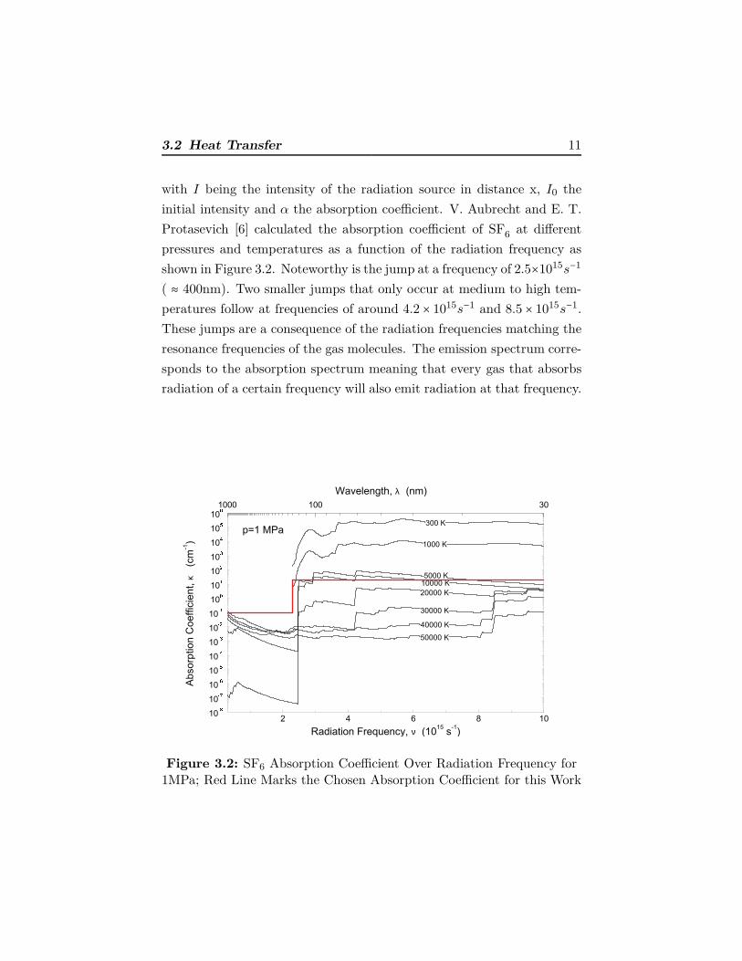
with I being the intensity of the radiation source in distance x, I0 the

initial intensity and α the absorption coefficient. V. Aubrecht and E. T.

Protasevich [6] calculated the absorption coefficient of SF6 at different

pressures and temperatures as a function of the radiation frequency as

shown in Figure 3.2. Noteworthy is the jump at a frequency of 2.5×1015s−1

( ≈ 400nm). Two smaller jumps that only occur at medium to high tem-

peratures follow at frequencies of around 4.2 × 1015s−1 and 8.5 × 1015s−1.

These jumps are a consequence of the radiation frequencies matching the

resonance frequencies of the gas molecules. The emission spectrum corre-

sponds to the absorption spectrum meaning that every gas that absorbs

radiation of a certain frequency will also emit radiation at that frequency.

κ

ν

λ

Figure 3.2: SF6 Absorption Coefficient Over Radiation Frequency for1MPa; Red Line Marks the Chosen Absorption Coefficient for this Work

12 3 Physics of Internal Arcs

Conduction plays a comparatively small role in this work’s simulations

due to the short time the arc is burning for. Furthermore, conduction is

disabled completely at the walls as they are treated adiabatically.

3.3 Electrode Erosion

The casing as well as the internal conductor, both manufactured from

aluminum, have a melting point of around 933°K. As the arc burns con-

siderably hotter than that at 20,000°K, puddles of molten aluminum form

at the arc roots. Two different processes account for the erosion:

• Vaporization of molten aluminum

• Droplet emission from the puddles of molten aluminum

Under the influence of the arc, a part of the molten aluminum is va-

porized instantaneously. Furthermore, the gas flow and the volumetric

expansion of the aluminum cause small droplets of molten aluminum to

splash away from the puddles as visualized in Figure 3.3.

Molten Aluminum

Expansion Shock Wave

Aluminum Droplets

Figure 3.3: Vaporization at the Arc Roots

3.4 Chemical Reactions 13

Due to their high surface to volume ratio, parts of these droplets are

vaporized by the arc before they can condense at colder surfaces of the

casing. This process of melting and vaporizing extracts large amounts

of energy from the arc (for aluminum: enthalpy of fusion = 397kJ/kg,

enthalpy of vaporization = 10526kJ/kg). Furthermore, the resulting alu-

minum vapor has the aforementioned temperature of 933°K and therefore

cools the arc. The modeling of the erosion process is discussed in section

4.1.4.

3.4 Chemical Reactions

Chemical reactions have a significant influence on the results of internal

arc simulations. This is due to the fact that the dissociation products

of SF6 and the vaporized electrode material react exothermically with

each other. This releases considerable amounts of energy that further

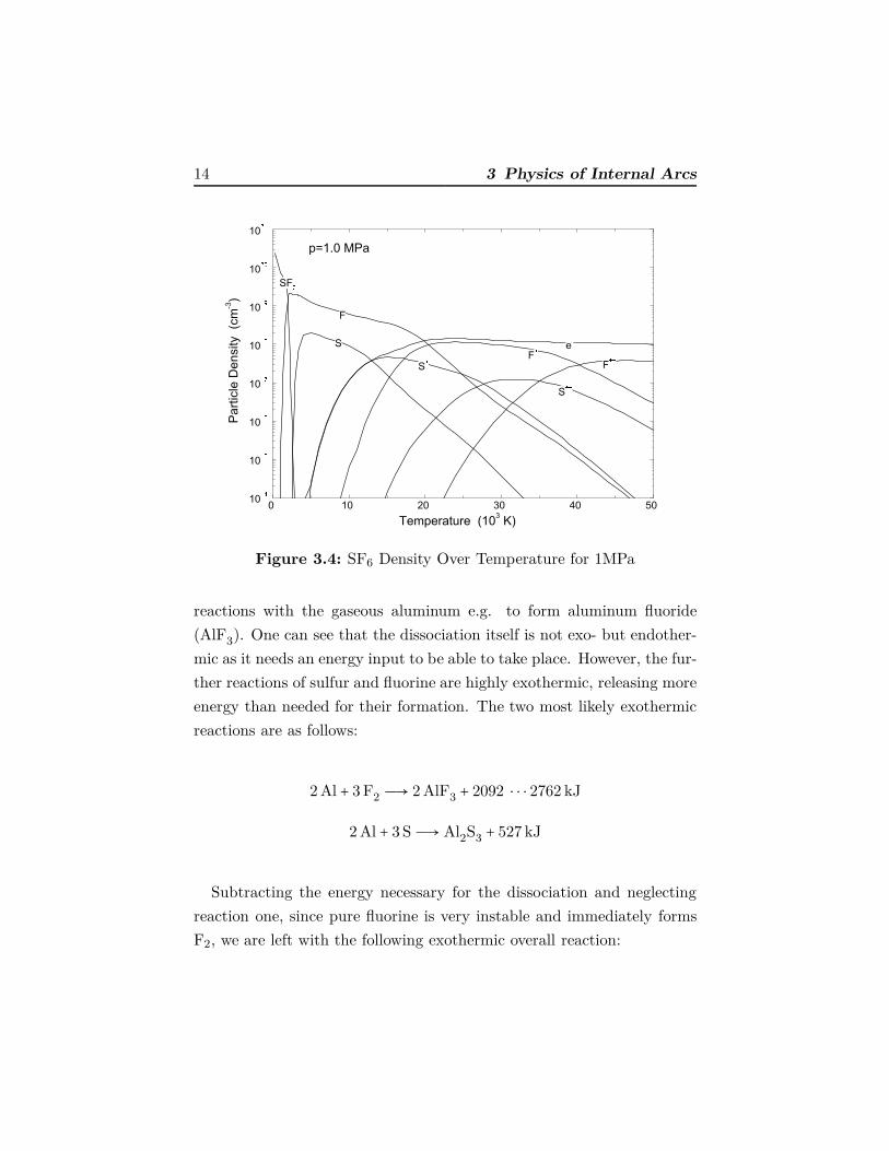
contribute to the heating of the gases. V. Aubrecht and E. T. Protasevich

showed that the dissociation of SF6 takes place at temperatures of around

1500K as shown in Figure 3.4.[6]

H. Schuhmann [7] set up the possible dissociations and reactions of

SF6 and aluminum vapor in his PhD thesis. The following two chemical

equations are the possible dissociations of SF6.

SF6 Ð→ S + 6 F−2210 kJ

SF6 Ð→ S + 3 F2−1097 ⋅ ⋅ ⋅ 1210 kJ

Parts of these dissociation products will form SF6 again immediately

which is called self healing and is a favorable property of SF6 (as men-

tioned in section 2.4). The remaining products will engage in chemical

14 3 Physics of Internal Arcs

Figure 3.4: SF6 Density Over Temperature for 1MPa

reactions with the gaseous aluminum e.g. to form aluminum fluoride

(AlF3). One can see that the dissociation itself is not exo- but endother-

mic as it needs an energy input to be able to take place. However, the fur-

ther reactions of sulfur and fluorine are highly exothermic, releasing more

energy than needed for their formation. The two most likely exothermic

reactions are as follows:

2 Al + 3 F2 Ð→ 2 AlF3 + 2092 ⋅ ⋅ ⋅ 2762 kJ

2 Al + 3 SÐ→ Al2S3 + 527 kJ

Subtracting the energy necessary for the dissociation and neglecting

reaction one, since pure fluorine is very instable and immediately forms

F2, we are left with the following exothermic overall reaction:

3.4 Chemical Reactions 15

8 Al + 3 SF6 Ð→ 6 AlF3 +Al2S3 + 5522 kJ

H. Schuhmann calculates that a specific energy of 11.9 kJ/g (grams of

burned aluminum) is released. This is a maximum possible energy that

is not reached in reality. Other reactions between sulfur, aluminum and

fluorine are possible and a considerable amount of energy is used to melt

aluminum without vaporizing it.

The actual chemical reactions are not simulated in this work but the

exothermic heat release is included in the real gas material data, described

in section 4.1.2.

4 Modeling

4.1 Physical Modeling

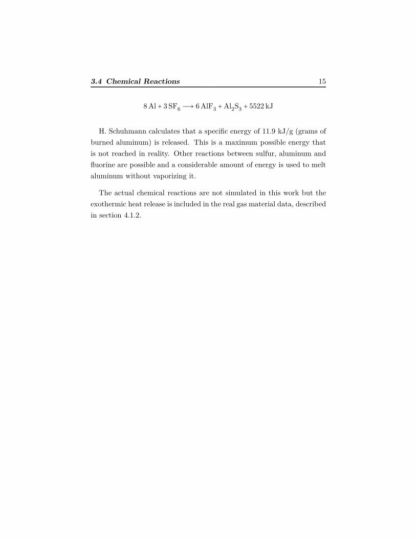
Figure 4.1 gives an overview over the main effects that occur during an

internal arc fault. This chapter will explain which effects were included

into the arc model and how this was done.

Outflow

Exothermic Reaction SF6\Al

Heat Transfer- Convection- Radiation- Conduction

Ohmic Heating

Contact Erosion- Vaporization- Droplet Emission

Magnetic Forces

Figure 4.1: Effects of an Internal Arc Fault

4.1.1 Arc Model

When simulating electric arcs a resolved arc model and an arc volume

model approach are possible. They are fundamentally different, both

having advantages and disadvantages as explained in this chapter.

18 4 Modeling

Resolved Arc Model

A resolved arc model can be based on the magnetohydrodynamic (MHD)

equations which consist of the Navier-Stokes equations extended by

Maxwell’s equations, see eg M. Torrhilon [8]. While the Navier-Stokes

equations take care of the fluid dynamics, Maxwell’s equations are neces-

sary to describe the electric and magnetic fields generated by the arc. As

in reality, the arc between anode and cathode forms due to an electric po-

tential between them. Phenomena that are included in these simulations

are the electric and magnetic field exerting forces on the fluid, ionization,

dissociation and plasma formation etc.. This kind of simulation was not

feasible for a long time since the high degree of freedom in such a sophis-

ticated arc model makes it extremely complicated and computationally

costly. Furthermore, it requires a highly resolved mesh in and around the

arc to be able to describe extreme gradients without numerical instability.

ABB has been running simulations like this for a few years, but both the

setup and computation is still very time consuming. As this work is not

focusing on the arc itself but on its effects regarding pressure build up, a

resolved arc model would have been too time consuming without yielding

considerable advantages. Therefore a non resolved arc volume model was

chosen.

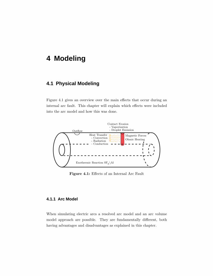
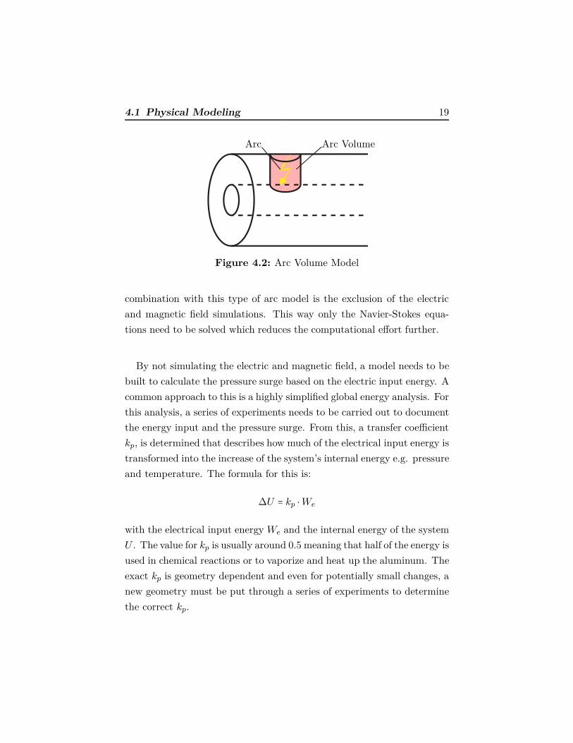
Arc Volume Model

In an arc volume model the arc is not resolved as such but described

through a larger volume that is placed around the arc, see Figure 4.2.

Since this volume is much larger than the arc itself, gradients at its

boundaries are a lot smaller, thus allowing coarser meshes and consider-

ably faster simulations. Another simplification that is commonly used in

4.1 Physical Modeling 19

Arc Arc Volume

Figure 4.2: Arc Volume Model

combination with this type of arc model is the exclusion of the electric

and magnetic field simulations. This way only the Navier-Stokes equa-

tions need to be solved which reduces the computational effort further.

By not simulating the electric and magnetic field, a model needs to be

built to calculate the pressure surge based on the electric input energy. A

common approach to this is a highly simplified global energy analysis. For

this analysis, a series of experiments needs to be carried out to document

the energy input and the pressure surge. From this, a transfer coefficient

kp, is determined that describes how much of the electrical input energy is

transformed into the increase of the system’s internal energy e.g. pressure

and temperature. The formula for this is:

∆U = kp ⋅We

with the electrical input energy We and the internal energy of the system

U . The value for kp is usually around 0.5 meaning that half of the energy is

used in chemical reactions or to vaporize and heat up the aluminum. The

exact kp is geometry dependent and even for potentially small changes, a

new geometry must be put through a series of experiments to determine

the correct kp.

20 4 Modeling

Since such a process is very undesirable, companies aim to include more

phenomena into the simulation, thus eventually eliminating the need for a

transfer coefficient. This was done in the course of this work. The power

input into the arc volume was calculated as follows:

Pinput = Pel − Pvap + Pinner

with the electrical input energy Pel, the energy used for the vaporization

of aluminum Pvap and the inner energy of the vaporized aluminum Pinner.

These are defined as follows:

Pel = Uarc ⋅ Iarc

Pvap =∆Hvap ⋅ mvap

Pinner =∆Hinner ⋅ mvap

with Uarc and Iarc being the arc voltage and current, ∆Hvap the enthalpy

of vaporization for aluminum and ∆Hinner the inner enthalpy of vaporized

aluminum. The mass vaporization rate of aluminum mvap is defined as:

mvap = cvap ⋅ Iarc

where cvap is a vaporization constant explained in section 4.1.4. The mass

vaporization rate of aluminum mvap is furthermore used as a mass input

into the arc volume. It is treated as a second species and interacts with the

SF6 as described in section 3.4. The inclusion of aluminum vaporization

into the arc model not only improves its results but also helps to stabilize

it in two ways.

• In the energy equation it accounts for Pvap and Pinner with Pvap >

Pinner. In total these extract energy from the arc that is not avail-

able for heating. This means that the arc does not get as hot as it

would without vaporization which helps the stability.

4.1 Physical Modeling 21

• Constantly injecting mass into the arc prevents the density inside

the arc from getting too close to zero which would lead to a crash.

This would happen since the extreme temperatures and pressures

inside the arc drive the gas away from it and the magnetic forces

that would hold the arc together in reality are neglected in this arc

model.

4.1.2 Gas Model

A real gas model was used in the course of this work to simulate the

behavior of the SF6/Al mixture. This was necessary since an ideal gas

model cannot accurately represent gas behavior in the case of an internal

arc fault.

Ideal gas models are based on a set of randomly moving particles mod-

eled as point masses that only interact with each other via elastic colli-

sions. These point masses obey the ideal gas law, pV = nRT , which can

be used to approximate most real gases at standard pressure and temper-

ature conditions. High temperatures and low pressures as well as light

gases generally favor this approximation because the size of the molecules

is less significant compared to the distance between them and the work

against intermolecular forces is less relevant compared with the particles’

kinetic energy.[9]

At extreme pressures, around condensation and critical points and to

explain phenomena like the Joule-Kelvin effect, a real gas model is nec-

essary to simulate molecules that have an actual size and interact with

more than just collisions, e.g. van der Waals forces. Other effects that

are considered by a real gas model are:

• compressibility

22 4 Modeling

• variable mechanical and chemical properties such as viscosity and

specific heat capacity

• non-equilibrium thermodynamic effects

• molecular dissociation and elementary reactions with variable com-

position

Since the pressure inside the bus bar casing is very high and SF6 is a

heavy gas (around 5 times heavier than air, see table 2.1), it does not

behave like an ideal gas. Furthermore, dissociation above 1500K (see

Figure 3.4), extreme calefaction and mixing with vaporized aluminum

from the casing considerably change the chemical and mechanical prop-

erties of SF6. The aforementioned factors raise the need for real gas data.

This data was available in the form of lookup tables giving values for

the density, enthalpy, entropy, speed of sound, thermal conductivity and

viscosity as functions of the temperature, pressure and the SF6/Al ratio.

The data for the enthalpy included the energy available from the exother-

mic reaction between SF6 and Al. All material properties were obtained

using the ABB chemical kinetics software Canthor which is based on the

open-source toolkit Cantera.[10]

4.1.3 Radiation Model

In contrast to the aforementioned gas properties, no lookup tables for the

absorption coefficient of a SF6/Al mixture were available. This is due to

the fact that the absorption coefficient, especially at extreme pressures

and temperatures, is extremely hard to determine in experiments. At the

time of this work, the only available lookup tables at ABB were for air.

However, from publications like V. Aubrecht’s and E. T. Protasevich’s

[6], the absorption coefficient as a function of the radiation frequency,

4.1 Physical Modeling 23

pressure and temperature is known, see Figure 3.2. They state that for

temperatures under 1000K and wavelengths over 400nm, absorption is

too small to be accurately determined and certainly small enough to be

neglected. At higher temperatures, the absorption coefficient increases as

well. For this work it was therefore estimated with a value of α = 10m−1.

For shorter wavelengths < 400nm, a value of α = 2000m−1 was chosen

considering the expected pressure and temperature inside the casing. The

chosen absorption frequencies are shown in red in Figure 3.2. As gases

emit photons at the same frequency at which they absorb them, emission

is implemented based on the same data.

More than two wavelength sections are possible which, at least at the

very high temperatures (> 20000K) inside the arc, would help to improve

accuracy but even then, this approach is an extreme simplification. It

is one of the main issues that should be addressed when a more precise

simulation of the internal arc fault is carried out in the future.

4.1.4 Erosion Model

As mentioned in section 4.1.1, the mass rate of vaporization for the elec-

trode material is related to the current flowing through the arc. In previ-

ous experiments carried out by ABB, the constant of proportionality cvap

for this relation was found to be bound by the following values:

2∆Ueff

∆Hvap

≤ cvap ≤

2∆Ueff

∆Hfue

where ∆Hfue and ∆Hvap are the enthalpies of fusion and vaporization

of the electrode material and ∆Ueff the effective voltage drop at the arc

root.

24 4 Modeling

The literature gives values of ∆Hfue = 397kJ/kg and ∆Hvap = 10526kJ/kg

for aluminum, while ∆Ueff = 10V was determined in experiments. How-

ever, these experiments involved copper electrodes and should therefore

be redone when the model is compared to aluminum benchmark cases.

The following boundaries for the proportionality factor are obtained based

on the copper experiments:

1.9 × 10−6≤ cvap ≤ 5 × 10−5 [ kg

As]

The lower boundary represents a case in which material is only ablated

due to vaporization, whereas the upper boundary describes a case where

the wear of the electrodes is heavily influenced by the emission of droplets

that are then partially vaporized. The model calculates the exact cvap

within this range based on the arc current, the arc duration and the

contact area between arc and electrode material. This resulted in a cvap

of 1.2 × 10−5 for the simulations in this work with the aforementioned

restriction that ∆Ueff is based on a copper electrode.

4.1.5 Arc Movement

Due to magnetic and electric forces as well as fluid motion, the arc inside a

bus bar moves along the axial and circumferential axes. To investigate the

influence of the arc’s position within the bus bar, a series of simulations

with different positions was carried out as part of this work. Due to the

2D axisymmetric approach, this variation was only possible along the

axial axis.

For more precise simulations, actual arc movement has to be included

into the simulation in the future. As mentioned in section 4.1.1 magnetic

and electric forces acting on the arc are unknown in this model. How-

ever equations to estimate these forces in combination with averaging

4.2 Numerical Modeling 25

the fluid’s velocity inside the arc volume and moving it accordingly is a

possible approach.

4.2 Numerical Modeling

4.2.1 Computational Fluid Dynamics

Fluid dynamics is the study of fluids and fluid motion under the influence

of forces. Computational fluid dynamics (CFD) utilizes numerical meth-

ods and algorithms to solve and analyze fluid dynamics problems. With

increasing computational power, this can be done for more mathemati-

cally complex problem sets that cannot be solved using analytical meth-

ods. Compared to experiments, CFD has the potential to save money,

time and resources and enables the analysis of phenomena that are not

reproducible in a laboratory (extreme heat and pressure, extremely large

or small geometries etc.).

For this work, the software Fluent by Ansys was used. Fluent is a

sophisticated CFD tool which is able to simulate sub and super sonic

flows, turbulence, heat transfer, component mixing.

4.2.2 Flow Numerics

The common approach to flow and combustion problems is the finite

volume method (FVM). The simulated geometry is divided into small

volumes (cells) for each of which a set of governing partial differential

equations is solved to describe the flow inside the cell. These so called

26 4 Modeling

Navier-Stokes equations typically consist of the conservation of mass, con-

servation of momentum and conservation of energy as listed below:

∂ρ

∂t+∇ ⋅ (ρv) = Sm

∂

∂t(ρv) +∇ ⋅ (ρvv) = −∇p +∇ ⋅ (τ) + ρg + F

∂

∂t(ρE) +∇ ⋅ (v (ρE + p)) = −∇ ⋅ ⎛⎝∑j hjJj

⎞⎠ + Sh

with density ρ, fluid velocity v, mass source terms Sm, static pressure

p, stress tensor τ , gravitational and external forces ρg and F , energy E,

specific enthalpy hj , diffusion flux of species j Jj and energy source terms

Sh. [11] [12]

4.2.3 Gas Numerics

The tables mentioned in section 4.1.2 are used by Fluent to update the

gas properties e.g. density and viscosity during every time step and for

each cell separately. Furthermore, Fluent is capable of modeling the mix-

ing and transport of chemical species by solving conservation equations

describing convection, diffusion, and reaction sources for each component

species. The convection-diffusion equation used to predict the local mass

fraction of each species Yi has the following general form:

∂

∂t(ρYi) +∇ ⋅ (ρvYi) = −∇ ⋅ Ji +Ri

where Ri is the net rate of production of species i through electrode

erosion and Ji the diffusion flux of species i.[12][11]

4.3 Meshing and Case Setup 27

4.2.4 Radiation Model

C. Luders states in his PhD thesis [13] that the P1 radiation model is an

efficient method to simulate radiation in combination with a CFD solver.

In comparison to other radiation transport models such as the discrete

ordinates model (DOM) it delivers acceptable results with considerably

less computational effort. The P1 model is based on the more general

P-N radiation model which uses the expansion of the radiation intensity

into an orthogonal series of spherical harmonics. Simplifying it by only

taking the first four terms in the series for gray radiation into account,

the following equation for the radiation flux, qr, is obtained:

qr = −1

3 (α +αs) −Cαs

∇G

with absorption coefficient α, scattering coefficient αs, incident radiation

G and linear anisotropic phase function coefficient C. [12][11]

4.3 Meshing and Case Setup

4.3.1 Meshing

The model for this simulation is an extremely simplified version of a

real bus bar. It includes the internal conductor and the enclosure and

considers both to be cylindrical. All changes in the diameter or shape of

the cylinders as well as any irregularities in the geometry such as bulkhead

seals are neglected. Bus bars are between 5m and 6m long and have inner

radii varying between 0m and 0.15m and outer radii between 0.1m and

0.3m.

28 4 Modeling

Meshing the bus bar in 2D meant that all axisymmetric features such

as the arc and the burst disk could not be accurately represented. As a

result, the arc was disk shaped with a hole in the middle (similar to the

shape of a CD). The inner and outer radii corresponded to the radius of

the internal conductor and the casing, respectively. The thickness of the

arc was 0.04m corresponding to its diameter which meant that the arc

volume was increased considerably. The reason for this is that a higher

arc volume causes a lower volumetric energy input into the arc. This

decreases the gradients at the arc volume edges and therefore increases

numerical stability. Furthermore, smaller gradients meant that a more

coarse mesh was sufficient which speeds up the simulation. Since the

focus of this work was not on the arc itself the arc volume change was

acceptable. The comparison of the 2D and 3D geometries is shown in

Figure 4.3b.

Casing (wall)

Internal Conductor (wall)

Arc Volume

Burst Disk

Fluid Volume

(a) 3D

(b) 2D

Figure 4.3: Geometry Including Boundary Conditions

4.3 Meshing and Case Setup 29

All simulations where run on structured quadrilateral (2D) and hexa-

hedral (3D) meshes created with Ansys Gambit. Structured grids were

chosen because they are easy to generate for simple geometries and, com-

pared to automated unstructured grid generator tools, provide more con-

trol over the mesh. Furthermore, they are memory saving and produce

better results and convergence.[14] The 2D meshes had between 3000

and 10,000 cells with the equivalent 3D meshes having between 40 and

50 times more.

4.3.2 Boundary Conditions

Two separate volume and boundary regions were created in each grid to

represent the arc and burst disk as follows:

• arc volume region: To represent the part of the volume between

the internal conductor and enclosure where the energy and mass is

introduced.

• fluid volume region: To represent the rest of the volume.

• burst-disk boundary region: To represent the part of the wall

section that opens at 15bar to simulate the burst disk.

• wall boundary region: To represent the remaining walls of the

internal conductor and enclosure.

The boundary conditions and fluid zones are visualized in Figure 4.3a.

Both the burst-disk and wall boundary are initialized as adiabatic no-

slip walls. This means that no heat is transfered through them and the

fluid adjacent to the wall has no velocity. Mathematically, these Dirichlet

30 4 Modeling

(no-slip) and Neumann (adiabatic) boundary conditions are expressed

as:

vx = vy = vz = 0

∂T

∂⇀

n= 0

where vx,vy and vz are the velocity components at the wall and⇀

n the

normal vector on the wall boundary.

A script in Ansys Fluent was used to simulate the burst disk. The script

calculates the average pressure of all cells directly adjacent to the burst-

disk boundary region. When this average exceeds the burst disk’s opening

pressure of 1.5MPa for the first time, the boundary type is switched from

no-slip wall to pressure-outlet. After this happens once, it is not reversed

even if the average pressure falls below 1.5MPa. A pressure-outlet in

Fluent is realized by holding the layer of cells that is immediately adjacent

to the outlet at a constant pressure and temperature that represent the

environment the fluid is flowing into.[12] In this simulation, the insulation

gas from the bus bar is released into the atmosphere thus the pressure

and temperature were set to 0.1MPa and 300K respectively. The Fluent

script can be found in Appendix A.1.

4.3.3 Simulation Input

As mentioned in section 4.1.1 the power and mass input into the arc is

based on the arc voltage and current. In this work alternating current

(AC) was used. An AC current frequency as well as a current and voltage

amplitude were used to define the volumetric power and mass input rates

using an Ansys Fluent script. Figure 4.4 shows the resulting inputs for

a case where the current is switched off after 0.1s. The corresponding

4.3 Meshing and Case Setup 31

fluent script can be found in Appendix A.2.

0 0.05 0.1 0.150

1

2

3

4

5

6

7x 10

9

0 0.05 0.1 0.150

20

40

60

80

100

120

140

Time [s]

En

ergy

[Wm−

2]

Mass

[kgm−

2s−

1]

Figure 4.4: Volumetric Energy and Mass Input Rates, RMS Values inBold

5 Results and Analysis

5.1 2D vs 3D Pressure Surge

The first simulations were setup to investigate the pressure surge during

the initial phase of the arc, when the burst disk is closed. Table 5.1 shows

the setup of the arc model.

Geometry (Length × Radius) 1m × 0.3m

Current Amplitude 141,421 A

Voltage Amplitude 566 V

Arc Radius 0.02 m

AC Current Frequency 50 Hz

Arc Duration 0.1s

Table 5.1: Arc Model Setup, 2D vs 3D Pressure Surge Investigation

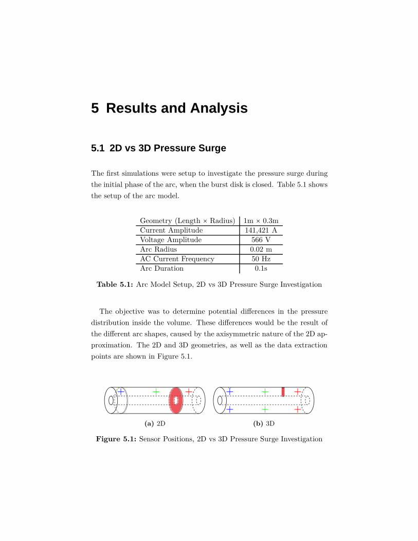
The objective was to determine potential differences in the pressure

distribution inside the volume. These differences would be the result of

the different arc shapes, caused by the axisymmetric nature of the 2D ap-

proximation. The 2D and 3D geometries, as well as the data extraction

points are shown in Figure 5.1.

(a) 2D (b) 3D

Figure 5.1: Sensor Positions, 2D vs 3D Pressure Surge Investigation

34 5 Results and Analysis

The temperature, density and pressure diagrams are shown in Figures

5.2 and 5.3.

0 0.02 0.04 0.06 0.08 0.10

1000

2000

3000

4000

5000

6000

7000

8000

9000

Time [s]

Tem

per

atu

re[K

]

0 0.02 0.04 0.06 0.08 0.10

5

10

15

20

25

30

Time [s]

Den

sity

[kgm−

3]

2D Arc 3D Arc 3D Arc Flipside

2D Center 3D Center 3D Center Flipside

2D Burst Disk 3D Burst Disk 3D Burst Disk Flipside

Figure 5.2: Temperature and Density Diagram, 2D vs 3D PressureSurge Investigation

As Figure 5.2 shows, the temperature and density curves only agree

at the data extraction point that is placed far away from the arc. The

3D simulation shows large differences between the data extraction points

placed in line with the arc and the ones placed on the opposite side of the

geometry. This difference decreases with a growing axial distance between

the arc and data extraction points. The results of the 2D model lie in

between the results of the respective data extraction point pair in 3D.

This is the result of the uniform energy distribution in the axisymmetric

arc volume.

5.2 2D vs 3D Outflow Function 35

0 0.01 0.02 0.03 0.04 0.05 0.06 0.07 0.08 0.09 0.10.5

1

1.5

2

2.5

3

3.5

4x 10

6

Time [s]

Pre

ssu

re[P

a]

2D Arc

3D Arc

3D Arc Flipside

2D Center

3D Center

3D Center Flipside

2D Burst Disk

3D Burst Disk

3D Burst Disk Flipside

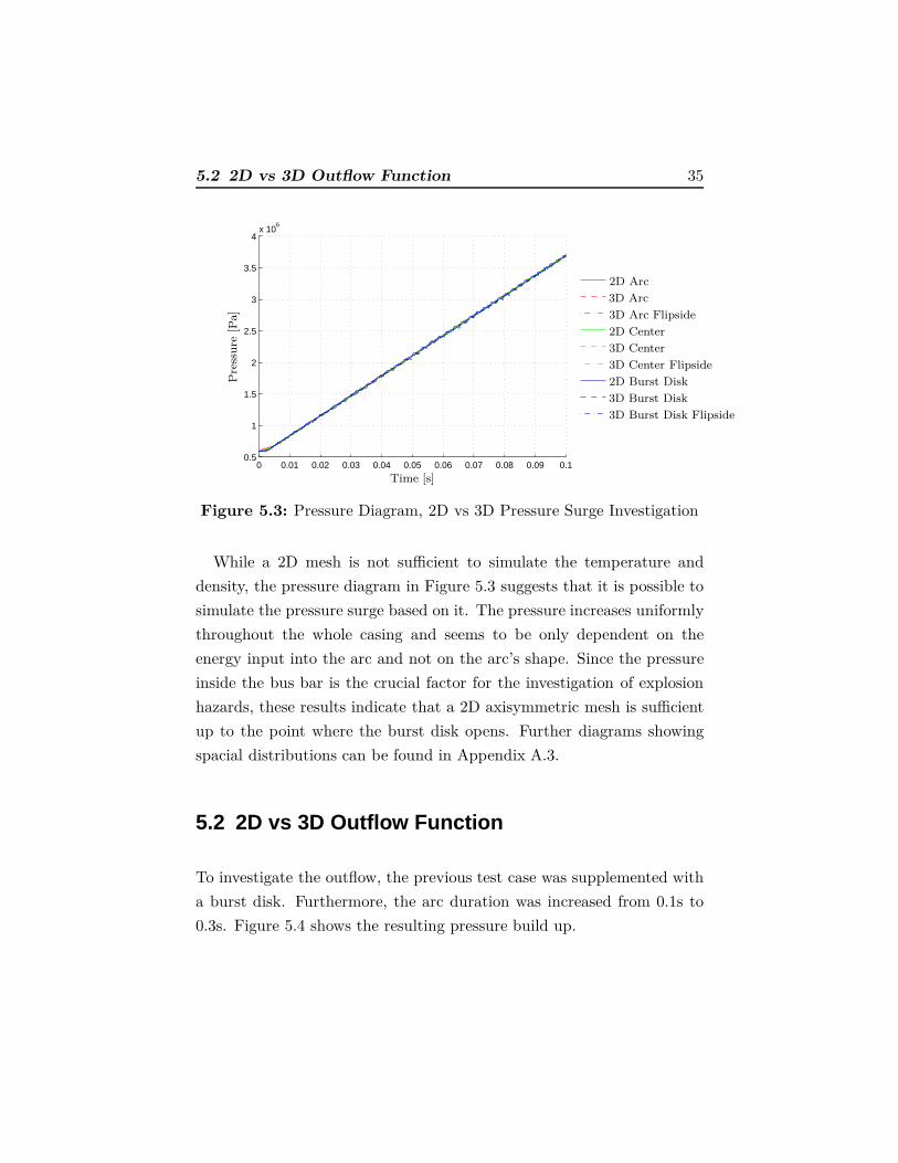
Figure 5.3: Pressure Diagram, 2D vs 3D Pressure Surge Investigation

While a 2D mesh is not sufficient to simulate the temperature and

density, the pressure diagram in Figure 5.3 suggests that it is possible to

simulate the pressure surge based on it. The pressure increases uniformly

throughout the whole casing and seems to be only dependent on the

energy input into the arc and not on the arc’s shape. Since the pressure

inside the bus bar is the crucial factor for the investigation of explosion

hazards, these results indicate that a 2D axisymmetric mesh is sufficient

up to the point where the burst disk opens. Further diagrams showing

spacial distributions can be found in Appendix A.3.

5.2 2D vs 3D Outflow Function

To investigate the outflow, the previous test case was supplemented with

a burst disk. Furthermore, the arc duration was increased from 0.1s to

0.3s. Figure 5.4 shows the resulting pressure build up.

36 5 Results and Analysis

0 0.05 0.1 0.15 0.2 0.25 0.3 0.35 0.40.5

1

1.5

2

2.5

3x 10

6

2D

3D

Burst Disk Opens Arc is Turned Off

Time [s]

Pre

ssu

re[P

a]

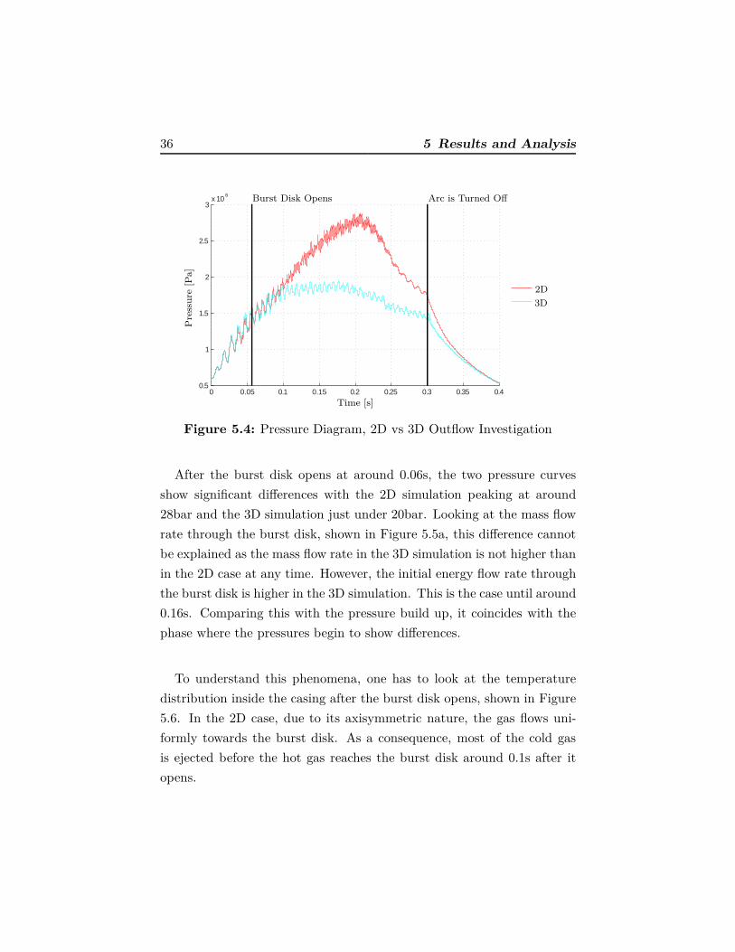
Figure 5.4: Pressure Diagram, 2D vs 3D Outflow Investigation

After the burst disk opens at around 0.06s, the two pressure curves

show significant differences with the 2D simulation peaking at around

28bar and the 3D simulation just under 20bar. Looking at the mass flow

rate through the burst disk, shown in Figure 5.5a, this difference cannot

be explained as the mass flow rate in the 3D simulation is not higher than

in the 2D case at any time. However, the initial energy flow rate through

the burst disk is higher in the 3D simulation. This is the case until around

0.16s. Comparing this with the pressure build up, it coincides with the

phase where the pressures begin to show differences.

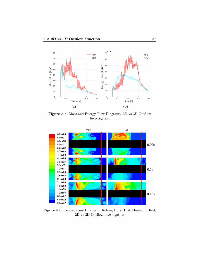
To understand this phenomena, one has to look at the temperature

distribution inside the casing after the burst disk opens, shown in Figure

5.6. In the 2D case, due to its axisymmetric nature, the gas flows uni-

formly towards the burst disk. As a consequence, most of the cold gas

is ejected before the hot gas reaches the burst disk around 0.1s after it

opens.

5.2 2D vs 3D Outflow Function 37

0 0.1 0.2 0.3 0.40

10

20

30

40

50

60

70

802D

3D

Time [s]

Mass

Flo

w[k

gs−

1]

(a)

0 0.1 0.2 0.3 0.40

10

20

30

40

50

60

702D

3D

x 103

Time [s]E

ner

gy

Flo

w[k

gK

s−1]

(b)

Figure 5.5: Mass and Energy Flow Diagrams, 2D vs 3D OutflowInvestigation

0.05s

0.1s

0.15s

2D 3D

Figure 5.6: Temperature Profiles in Kelvin, Burst Disk Marked in Red,2D vs 3D Outflow Investigation

38 5 Results and Analysis

In the 3D case, the arc volume has not heated up the gas uniformly

around the circumferential axis before the burst disk opens. After the

burst disk opens, the gas flow mainly sucks out the hot gases from around

the arc volume. These reach the burst disk much sooner than in the 2D

case which explains the higher initial energy flow rate. Using streamlines

to visualize the flow field for the 3D case, it was possible to see that

the colder gas from the bottom side of the bus bar is sucked around the

internal conductor. It then mixes with the hot gas. However, this flow

only develops in a certain distance to the burst disk and the lower right

half of the 3D case is not effected by it.

Changing the aspect ratio (length/radius) of the geometry from 3.33

to 20 by increasing its length from 1m to 3m and reducing its radius

from 0.3m to 0.15m, the section where no fluid flow occurs becomes less

significant. The pressure diagram obtained with the longer geometry is

shown in Figure 5.7.

0 0.05 0.1 0.150.5

1

1.5

2

2.5

3x 10

6

2D

3D

Burst Disk Opens Arc is Turned Off

Time [s]

Pre

ssu

re[P

a]

Figure 5.7: Pressure Diagram, 3m × 0.15m Geometry, 2D vs 3DOutflow Investigation

5.3 Burst Disk Modification 39

The pressure curves are much more similar with a difference of only

1bar at the pressure peak. After the arc is turned off this difference

increases. However, this is not important when investigating explosion

hazards and was therefore not further investigated in the course of this

work.

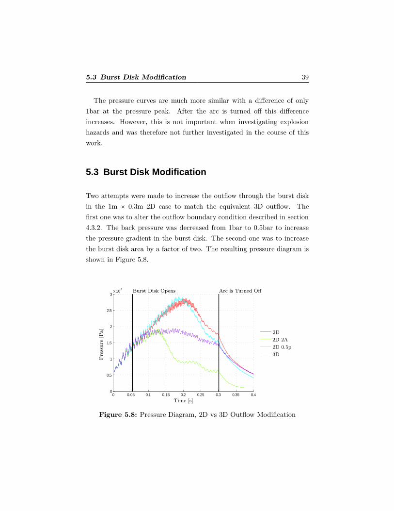
5.3 Burst Disk Modification

Two attempts were made to increase the outflow through the burst disk

in the 1m × 0.3m 2D case to match the equivalent 3D outflow. The

first one was to alter the outflow boundary condition described in section

4.3.2. The back pressure was decreased from 1bar to 0.5bar to increase

the pressure gradient in the burst disk. The second one was to increase

the burst disk area by a factor of two. The resulting pressure diagram is

shown in Figure 5.8.

0 0.05 0.1 0.15 0.2 0.25 0.3 0.35 0.40

0.5

1

1.5

2

2.5

3x 10

6

2D

3D

2D 2A

2D 0.5p

Burst Disk Opens Arc is Turned Off

Time [s]

Pre

ssu

re[P

a]

Figure 5.8: Pressure Diagram, 2D vs 3D Outflow Modification

40 5 Results and Analysis

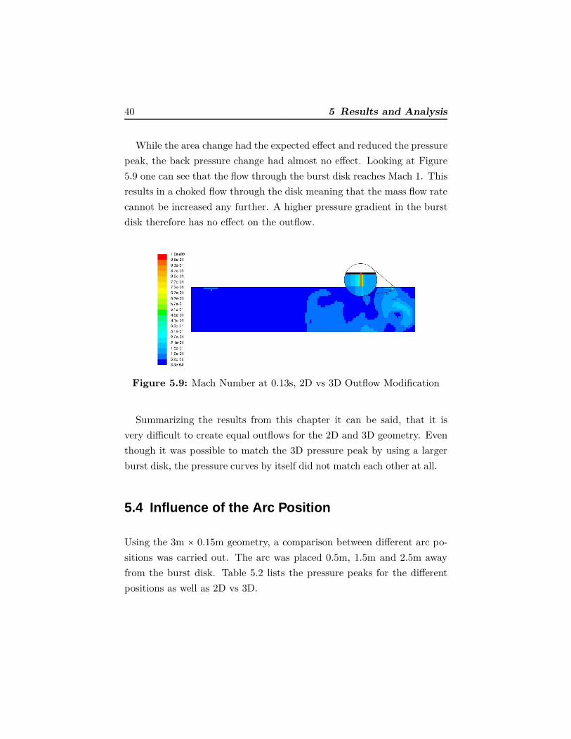
While the area change had the expected effect and reduced the pressure

peak, the back pressure change had almost no effect. Looking at Figure

5.9 one can see that the flow through the burst disk reaches Mach 1. This

results in a choked flow through the disk meaning that the mass flow rate

cannot be increased any further. A higher pressure gradient in the burst

disk therefore has no effect on the outflow.

Figure 5.9: Mach Number at 0.13s, 2D vs 3D Outflow Modification

Summarizing the results from this chapter it can be said, that it is

very difficult to create equal outflows for the 2D and 3D geometry. Even

though it was possible to match the 3D pressure peak by using a larger

burst disk, the pressure curves by itself did not match each other at all.

5.4 Influence of the Arc Position

Using the 3m × 0.15m geometry, a comparison between different arc po-

sitions was carried out. The arc was placed 0.5m, 1.5m and 2.5m away

from the burst disk. Table 5.2 lists the pressure peaks for the different

positions as well as 2D vs 3D.

5.4 Influence of the Arc Position 41

Arc to Burst Disk Distance0.5m 1.5m 2.5m

2D 17bar 23bar 26bar

3D 17bar 27bar 27bar

Table 5.2: Pressure Peaks, Arc Position Investigation

Figures 5.11 and 5.11 show the corresponding pressure curves.

0 0.05 0.1 0.150

0.5

1

1.5

2

2.5

3x 10

6

0.5m

1.5m

2.5m

Burst Disk Opens Arc is Turned Off

Time [s]

Pre

ssu

re[P

a]

Figure 5.10: 2D Pressure Diagram, Burst Disk Opening Times areSlightly Different for All Cases, Arc Position Investigation

While the 1.5m and 2.5m cases show a similar peak pressure, it is

significantly lower in the 0.5m case. This is important since the gas flow

after the burst disk opens carries the arc towards the burst disk. This

makes arc movement a key factor that cannot be neglected. In the course

of this work the implementation of are movement based on the average gas

velocity inside the arc was started but could not be finished in time.

42 5 Results and Analysis

0 0.05 0.1 0.150.5

1

1.5

2

2.5

3x 10

6

0.5m

1.5m

2.5m

Burst Disk Opens Arc is Turned Off

Time [s]

Pre

ssu

re[P

a]

Figure 5.11: 3D Pressure Diagram, Burst Disk Opening Times areSlightly Different for All Cases, Arc Position Investigation

6 Conclusion

In the course of this work, a model for the simulation of the pressure

surge due to internal arc faults in GIS was developed. Summarizing the

results, the following two key statements can be made:

• It is generally possible to use 2D axisymmetric meshes for the simu-

lation of the pressure build up during internal arc faults in bus bars.

Very good conformity between the 2D and 3D pressure simulations

is achieved during the first phase of the simulation while the burst

disk is closed. For this phase the results based on a 2D mesh can

assumed to be reliable. For the second phase of the simulation, dur-

ing which the absolute pressure peak inside the casing is reached,

the geometry’s length to radius ratio should be higher than 10 to

achieve acceptable agreement between the 2D and 3D cases.

• Arc movement has a significant influence on the pressure build up

and peak pressure inside the casing. As the results in the previous

chapter show, the peak pressure is lower when the arc stands closer

to the burst disk. This difference is especially large when the arc

is closer than 0.5m to the burst disk. The arc model at its current

state can therefore only deliver realistic results when the arc occurs

close to the burst disk.

To improve the arc model further, ABB will include arc movement into the

arc model as a next step. This will be realized as described in section 4.1.5.

Another approach that is currently investigated is the further reduction of

dimensions from 2D to 1D. This would reduce simulation times to under

one hour. Even though the 1D model is still in an early test phase, its

results compared to the 2D model look promising.

Bibliography

[1] S. Kobayashi D. Kopejtkove T. Molony P. O’Connell B. Skyberg J.

P. Taillebois I. Welch C. N. Cheung, F. Heil. Report on the second

international survey on high voltage gas insulated substations (gis)

service experience. Cigre Brochure, 2000.

[2] Matthey SA. Membranes, snap domes and bursting discs, tech-

nical file. http://www.matthey.ch/en/applications/membranes-and-

bursting-disks/, 2013.

[3] D. Koch. Sf6 properties, and use in mv and hv switchgear. Technical

report, Cahier technique no. 188, 2003.

[4] Intergovernmental Panel on Climate Change. 6.12.2 direct gwps,

2001.

[5] R. Luchtenberg H. Picard, J. Verstraten. Practical approaches to

mitigating arc flash exposure in europe. Technical report, PCIC

Europe, 2013.

[6] E. T. Protasevich V. Aubrecht. Radiative transport of energy in sf6

arc plasma. Technical report, Brno University of Technology, Tomsk

Polytechnical University, 2000.

[7] H. Schuhmann. Untersuchungen zum Druckanstieg in Schottraumen

SF6-isolierter, einpolig metallgekapseler Hochspannungs Schaltan-

lagen infolge stromstarker Storlichtbogen. PhD thesis, Technische

Hochschule Darmstadt, 1989.

[8] M. Torrilhon. Zur Numerik der Idealen Magnetohydrodynamik. PhD

thesis, Eidgenossische Technische Hochschule Zurich, 2003.

II Bibliography

[9] M.A. Boles Y.A. Cengel. Thermodynamics: An Engineering Ap-

proach. 2002.

[10] K. Hencken C. Doiron. Calculation of thermodynamic and transport

properties of thermal plasmas based on the cantera software toolkit.

Technical report, ABB Corporate Research Switzerland, 2014.

[11] Ansys Inc. ANSYS FLUENT User Guide, 2014.

[12] Ansys Inc. ANSYS FLUENT Theory Guide, 2014.

[13] C. Luders. Vergleich von Strahlungs- und Turbulenzmodellen zur

Modellierung von Lichtbogen in SF6 Selbstblasleistungsschaltern.

PhD thesis, Rheinisch-Westfalische Technische Hochschule Aachen,

2005.

[14] John Chawner. Quality and control - two reasons why structured

grids aren’t going away. Pointwise - The Connector, 2013.

A Appendix

A.1 Burst Disk Script

1 ( d e f i n e ( burst −setup )

2 ( l e t ∗ ( ( pavg 6e5 ) ; [ Pa ]

3 ( p av g c r i t 15 e5 ) ; [ Pa ]

4 ( t imestep 0) ; [ s ]

5 ( time 0) )

6

7 ( s e t ! time ( rpgetvar ’ f low −time ) )

8 ( s e t ! t imestep ( rpgetvar ’ phys i ca l −time− s tep ) )

9 ( s e t ! pavg ( g e t s u r f av g ’ ( b u r s t d i s k ) ’ p r e s su r e ) )

10

11 ( i f (member ’ b u r s t d i s k ( c l i e n t − i nqu i r e −zones−of −type ’ wal l ) ) ; ⤦

Ç i f b u r s t d i s k i s o f type wal l

12 ( i f (>= pavg p av g c r i t )

13 ( begin

14 ; s e t b u r s t d i s k from wal l to p r e s su r e o u t l e t

15 ( t i −menu− load − s t r i n g ( format #f ⤦

Ç ”˜%/ d e f i n e /boundary− con d i t i on s /zone−type b u r s t d i s k ⤦

Ç pressure − o u t l e t ˜%”) )

16 ; s e t p r e s su r e o u t l e t b . c . f o r b u r s t d i s k

17 ( t i −menu− load − s t r i n g

18 ( format #f ”˜a˜%˜a˜%˜a˜%˜a˜%˜a˜%˜a˜%˜a˜%˜s˜%˜s˜%˜a˜%˜a˜% ⤦

Ç ˜a˜%˜a˜%˜a˜%˜a˜%˜a˜%˜a˜%˜a˜%˜a˜%”

19 ”/ d e f i n e /boundary− con d i t i on s ”

20 ” pres sure −o u t l e t ”

21 ” b u r s t d i s k ” ; zone id /name

22 ”no” ; Use P r o f i l e f o r Gauge Pressure ?

23 ”1 e5 ” ; Gauge Pressure ( pas ca l ) [ 0 ] 1 e5

24 ” yes ” ; Use P r o f i l e f o r Backflow Total Temperature ?

25 ” yes ” ; Use UDF P r o f i l e f o r Backflow Total Temperature?

26 ” udf ” ; p r o f i l e name

27 ” backflow T : : l i b u d f ” ; data name

IV A Appendix

28 ”no” ; Backflow Dir ec t i on S p e c i f i c a t i o n Method : Di r ec t i on ⤦

Ç Vector

29 ” yes ” ; Backflow Dir ec t i on S p e c i f i c a t i o n Method : Normal to ⤦

Ç Boundary

30 ” yes ” ; External Black Body Temperature Method : Boundary ⤦

Ç Temperature

31 ”no” ; Use P r o f i l e f o r I n t e r n a l Emis s iv i ty ?

32 ”1” ; I n t e r n a l Emis s iv i ty

33 ”no” ; Spec i f y Spec i e s in Mole Fract i on s ?

34 ”no” ; Use P r o f i l e f o r s f 6 f r a c t i o n ?

35 ”1” ; s f 6 f r a c t i o n

36 ”no” ; Spec i f y Average Pressure S p e c i f i c a t i o n

37 ”no” ; Spec i f y targe ted mass f low rate

38 )

39 )

40 )

41 )

42 )

43 )

44 )

A.2 Power and Mass Input Script V

A.2 Power and Mass Input Script

1 /∗ Input parameters ∗/

2 #i f RP 3D

3 #d e f i n e v o l a r c 0.003375 /∗ Arc−volume in [mˆ3 ] ∗/

4 #e l s e

5 #d e f i n e v o l a r c 0.003375

6 #en d i f

7 #d e f i n e I RMS 12500 /∗ RMS cur r en t in [A] ∗/

8 #d e f i n e Qarc 252000 /∗ Total r e l e a s e d energy in [ J ] ∗/

9 #d e f i n e arct ime 0 .1 /∗ Arcing time in [ s ] ∗/

10 #d e f i n e f r eq 60 /∗ Frequency in [1/ s ] ∗/

11 #d e f i n e use kp 0 /∗ use Kp f a c t o r or not ∗/

12 #d e f i n e kp 0.53 /∗ Kp f a c t o r ∗/

13 #d e f i n e tau 0 .0 /∗ Delay time to reach f u l l input power ⤦

Ç [ s ] ∗/

14

15 /∗ Mater ia l Constants o f Aluminium ∗/

16 #d e f i n e SeegerNo 1 .2 e−5 /∗ dM/dt= SeegerNo∗ Current in [ kg/ s /A]∗/

17 #d e f i n e Kappa AL 1.66 /∗ Isentropenexponent Aluminium ∗/

18 #d e f i n e m AL 4.5 e−26 /∗ Atomic mass o f Alu ∗/

19 #d e f i n e de l ta E 10900000 /∗ Evaporation energy o f Alu in [ J/kg ]∗/

20 #d e f i n e T verd 2740 /∗ Evaporation temperatur o f Alu in [K]∗/

21

22 /∗ Other Constants ∗/

23 #d e f i n e Kb 1.38 e−23 /∗ Bolzmann Konstante in [ J/ s ] ∗/

24 #d e f i n e a b s c o e f f l i m 1 .0

25 #d e f i n e um rhodot 0

26 #d e f i n e um rhoedot 1

27 #d e f i n e um P el 2

28 #d e f i n e um P evap 3

29 #d e f i n e um P i 4

30

31 /∗ Mass source by e l e c t r o d e eros ion , c o n s i s t i n g o f evaporat ion and ⤦

Ç drop l e t emmission ∗/

32 DEFINE SOURCE( mass source , c , t , ds , eqn )

33 {

VI A Appendix

34 r e a l time = CURRENT TIME; /∗ time in seconds ∗/

35 r e a l rhodot ;

36 r e a l I t , U t , I peak , U peak , U;

37 r e a l P el , P i , P evap ;

38

39

40 I peak=s q r t (2 ) ∗I RMS ; /∗ Peak cu r r en t ∗/

41 I t = fab s ( I peak ∗ s i n (2∗M PI∗ f r eq ∗ time ) ) ; /∗ t r a n s i e n t Current ∗/

42

43 U= Qarc/ arct ime /I RMS ; /∗ RMS Voltage ∗/

44 U peak=s q r t (2 ) ∗U; /∗ Peak Voltage ∗/

45 U t = fabs ( U peak∗ s i n (2∗M PI∗ f r eq ∗ time ) ) ; /∗ t r a n s i e n t Voltage ∗/

46

47 P e l = ( U t ∗ I t ) ; /∗ Input e l e c t r i c a l Power in [W]∗/

48 P i = T verd∗Kb/(m AL∗(Kappa AL−1) ) ∗SeegerNo∗ I t ; /∗ Inner ⤦

Ç energy den s i ty o f evaporated Alu ∗ dm/dt in ⤦

Ç [ J/kg ] ∗ [ kg/ s /A] ∗ [A] = [W] ∗/

49 P evap = delta E ∗SeegerNo∗ I t ; /∗ energy r equ i r ed to evaporate ⤦

Ç Alu ∗ dm/dt in [ J/kg ] ∗ [ kg/ s /A] ∗ [A] = [W] ∗/

50 /∗ t o t a l power input = P e l + P i − P evap ∗/

51

52 /∗ choose e r o s i on such that the e r o s i on energy i s maximal h a l f o f ⤦

Ç the e l e c t r i c a l energy fab s ( P i −P evap ) <= P el /2 .0 ∗/

53 /∗ i f P e l < 2∗ fab s ( P i − P evap ) evaporate l e s s mater i a l ∗/

54 i f ( P e l / f ab s ( P i −P evap ) <2.0)

55 {

56 /∗ you can c a l c u l a t e P i and P evap by r e d e f i n i n g I t ∗/

57 /∗ i . e . ( T verd∗Kb/(m AL∗(Kappa AL−1) )−del ta E ) ∗SeegerNo∗ I t = ⤦

Ç P e l /2 .0 ∗/

58 /∗ <−> ( P i −P evap ) / I t = P e l /2 .0/ I t ∗/

59 I t = fab s ( P e l /2 .0 / ( P i −P evap ) ∗ I t ) ;

60 }

61

62 i f ( time <= tau ) rhodot = SeegerNo∗ I t / v o l a r c ∗( time / tau ) ; /∗ ⤦

Ç [ kg/ s /A] ∗ [A] / [mˆ3 ] = [ kg/mˆ3/ s ] ∗/

63 e l s e rhodot = SeegerNo∗ I t / v o l a r c ; /∗ ⤦

Ç [ kg/mˆ3/ s ] ∗/

A.2 Power and Mass Input Script VII

64

65 C UDMI( c , t , um rhodot ) = rhodot ; /∗ [Kg/mˆ3/ s ] ∗/

66

67 return rhodot ;

68 }

69

70 /∗ Energy source by e l e c t r i c power and e l e c t r o d e e r o s i on : Total ⤦

Ç power input = P e l + P i − P evap ∗/

71 DEFINE SOURCE( power source , c , t , ds , eqn )

72 {

73 r e a l time = CURRENT TIME; /∗ time in seconds ∗/

74 r e a l rhoedot ;

75 r e a l I t , U t , I peak , U peak , U;

76 r e a l P el , P i , P evap ;

77

78 I peak=s q r t (2 ) ∗I RMS ; /∗ Peak cu r r en t ∗/

79 I t = fab s ( I peak ∗ s i n (2∗M PI∗ f r eq ∗ time ) ) ; /∗ t r a n s i e n t Current ∗/

80

81 U=Qarc/ arct ime /I RMS ; /∗ RMS Voltage ∗/

82 U peak=s q r t (2 ) ∗U; /∗ Peak Voltage ∗/

83 U t = fabs ( U peak∗ s i n (2∗M PI∗ f r eq ∗ time ) ) ; /∗ t r a n s i e n t Voltage ∗/

84

85 /∗ t o t a l power input = P e l + P i − P evap ∗/

86 i f ( use kp )

87 {

88 P e l = kp∗( U t ∗ I t ) ; /∗ Input e l e c t r i c a l Power in [W]∗/

89 P i = 0 . 0 ;

90 P evap = 0 . 0 ;

91 }

92 e l s e

93 {

94 P e l = ( U t ∗ I t ) ; /∗ Input e l e c t r i c a l Power in [W]∗/

95 P i = T verd∗Kb/(m AL∗(Kappa AL−1) ) ∗SeegerNo∗ I t ; /∗ ⤦

Ç Inner energy den s i ty o f evaporated Alu ∗ dm/dt in ⤦

Ç [ J/kg ] ∗ [ kg/ s /A] ∗ [A] = [W] ∗/

96 P evap = delta E ∗SeegerNo∗ I t ; /∗ energy r equ i r ed to ⤦

Ç evaporate Alu ∗ dm/dt in [ J/kg ] ∗ [ kg/ s /A] ∗ [A] = [W] ∗/

VIII A Appendix

97

98 /∗ choose e r o s i on such that the e r o s i on energy i s maximal ⤦

Ç h a l f o f the e l e c t r i c a l energy fab s ( P i −P evap ) <= ⤦

Ç P e l /2 .0 ∗/

99 /∗ i f P e l < 2∗ fab s ( P i − P evap ) evaporate l e s s mater i a l ∗/

100 i f ( P e l / f ab s ( P i −P evap ) <2.0)

101 {

102 /∗ you can c a l c u l a t e P i and P evap by r e d e f i n i n g ⤦

Ç I t ∗/

103 /∗ ⤦

Ç i . e . ( T verd∗Kb/(m AL∗(Kappa AL−1) )−del ta E ) ∗SeegerNo∗ I t ⤦

Ç = P el /2 .0 ∗/

104 /∗ <−> ( P i −P evap ) / I t = P e l /2 .0/ I t ∗/

105 I t = fab s ( P e l /2 .0 / ( P i −P evap ) ∗ I t ) ;

106 P i = T verd∗Kb/(m AL∗(Kappa AL−1) ) ∗SeegerNo∗ I t ;

107 P evap = delta E ∗SeegerNo∗ I t ;

108 }

109 }

110

111 i f ( time <= tau ) rhoedot =(( P e l+P i −P evap ) / v o l a r c ) ∗( time / tau ) ; ⤦

Ç /∗ [ kg/mˆ3/ s ] ∗/

112 e l s e rhoedot =(( P e l+P i −P evap ) / v o l a r c ) ; ⤦

Ç /∗ [ kg/mˆ3/ s ] ∗/

113

114 C UDMI( c , t , um rhoedot ) = rhoedot ; /∗ [W/mˆ3 ] ∗/

115 C UDMI( c , t , um P el ) = P e l ;

116 C UDMI( c , t , um P evap ) = P evap ;

117 C UDMI( c , t , um P i ) = P i ;

118

119 return rhoedot ;

120 }

A.3 Spacial Diagrams, 2D vs 3D Pressure Surge Investigation IX

A.3 Spacial Diagrams, 2D vs 3D Pressure Surge Investigation

The following diagrams show spacial distribution inside the volume at 0.01s. The arc position is

marked in red.

Figure A.1

Figure A.2

X A Appendix

Figure A.3

Figure A.4

A.3 Spacial Diagrams, 2D vs 3D Pressure Surge Investigation XI

Figure A.5

Figure A.6