cfx reference guide · this ansys software product and program documentation include trade secrets...
TRANSCRIPT
ANSYS CFX Reference Guide
Release 15.0ANSYS, Inc.November 2013Southpointe
275 Technology DriveCanonsburg, PA 15317 ANSYS, Inc. is
certified to ISO9001:2008.
[email protected]://www.ansys.com(T) 724-746-3304(F) 724-514-9494
Copyright and Trademark Information
© 2013 SAS IP, Inc. All rights reserved. Unauthorized use, distribution or duplication is prohibited.
ANSYS, ANSYS Workbench, Ansoft, AUTODYN, EKM, Engineering Knowledge Manager, CFX, FLUENT, HFSS and anyand all ANSYS, Inc. brand, product, service and feature names, logos and slogans are registered trademarks ortrademarks of ANSYS, Inc. or its subsidiaries in the United States or other countries. ICEM CFD is a trademark usedby ANSYS, Inc. under license. CFX is a trademark of Sony Corporation in Japan. All other brand, product, serviceand feature names or trademarks are the property of their respective owners.
Disclaimer Notice
THIS ANSYS SOFTWARE PRODUCT AND PROGRAM DOCUMENTATION INCLUDE TRADE SECRETS AND ARE CONFID-ENTIAL AND PROPRIETARY PRODUCTS OF ANSYS, INC., ITS SUBSIDIARIES, OR LICENSORS. The software productsand documentation are furnished by ANSYS, Inc., its subsidiaries, or affiliates under a software license agreementthat contains provisions concerning non-disclosure, copying, length and nature of use, compliance with exportinglaws, warranties, disclaimers, limitations of liability, and remedies, and other provisions. The software productsand documentation may be used, disclosed, transferred, or copied only in accordance with the terms and conditionsof that software license agreement.
ANSYS, Inc. is certified to ISO 9001:2008.
U.S. Government Rights
For U.S. Government users, except as specifically granted by the ANSYS, Inc. software license agreement, the use,duplication, or disclosure by the United States Government is subject to restrictions stated in the ANSYS, Inc.software license agreement and FAR 12.212 (for non-DOD licenses).
Third-Party Software
See the legal information in the product help files for the complete Legal Notice for ANSYS proprietary softwareand third-party software. If you are unable to access the Legal Notice, please contact ANSYS, Inc.
Published in the U.S.A.
Table of Contents
1. ANSYS CFX Launcher . . . . . . . . . . . . . . . . . . . . . . . . . . . . . . . . . . . . . . . . . . . . . . . . . . . . . . . . . . . . . . . . . . . . . . . . . . . . . . . . . . . . . . . . . . . . . . . . . . . . . . . . . . . . . . . . . . . . . . . . . . . . . . 11.1.The ANSYS CFX Launcher Interface .... . . . . . . . . . . . . . . . . . . . . . . . . . . . . . . . . . . . . . . . . . . . . . . . . . . . . . . . . . . . . . . . . . . . . . . . . . . . . . . . . . . . . . . . . . . . . . . . . 1
1.1.1. Menu Bar ... . . . . . . . . . . . . . . . . . . . . . . . . . . . . . . . . . . . . . . . . . . . . . . . . . . . . . . . . . . . . . . . . . . . . . . . . . . . . . . . . . . . . . . . . . . . . . . . . . . . . . . . . . . . . . . . . . . . . . . . . . . . . . . 11.1.1.1. File Menu .... . . . . . . . . . . . . . . . . . . . . . . . . . . . . . . . . . . . . . . . . . . . . . . . . . . . . . . . . . . . . . . . . . . . . . . . . . . . . . . . . . . . . . . . . . . . . . . . . . . . . . . . . . . . . . . . . . . . . 1
1.1.1.1.1. Save As .... . . . . . . . . . . . . . . . . . . . . . . . . . . . . . . . . . . . . . . . . . . . . . . . . . . . . . . . . . . . . . . . . . . . . . . . . . . . . . . . . . . . . . . . . . . . . . . . . . . . . . . . . . . . . . . . 11.1.1.1.2. Quit ... . . . . . . . . . . . . . . . . . . . . . . . . . . . . . . . . . . . . . . . . . . . . . . . . . . . . . . . . . . . . . . . . . . . . . . . . . . . . . . . . . . . . . . . . . . . . . . . . . . . . . . . . . . . . . . . . . . . . . 1
1.1.1.2. Edit Menu .... . . . . . . . . . . . . . . . . . . . . . . . . . . . . . . . . . . . . . . . . . . . . . . . . . . . . . . . . . . . . . . . . . . . . . . . . . . . . . . . . . . . . . . . . . . . . . . . . . . . . . . . . . . . . . . . . . . . 21.1.1.2.1. Clear ... . . . . . . . . . . . . . . . . . . . . . . . . . . . . . . . . . . . . . . . . . . . . . . . . . . . . . . . . . . . . . . . . . . . . . . . . . . . . . . . . . . . . . . . . . . . . . . . . . . . . . . . . . . . . . . . . . . . . 21.1.1.2.2. Find .... . . . . . . . . . . . . . . . . . . . . . . . . . . . . . . . . . . . . . . . . . . . . . . . . . . . . . . . . . . . . . . . . . . . . . . . . . . . . . . . . . . . . . . . . . . . . . . . . . . . . . . . . . . . . . . . . . . . . 21.1.1.2.3. Options .... . . . . . . . . . . . . . . . . . . . . . . . . . . . . . . . . . . . . . . . . . . . . . . . . . . . . . . . . . . . . . . . . . . . . . . . . . . . . . . . . . . . . . . . . . . . . . . . . . . . . . . . . . . . . . . 2
1.1.1.2.3.1. User Interface Style .... . . . . . . . . . . . . . . . . . . . . . . . . . . . . . . . . . . . . . . . . . . . . . . . . . . . . . . . . . . . . . . . . . . . . . . . . . . . . . . . . . . . . 21.1.1.2.3.2. Application Font and Text Window Font .... . . . . . . . . . . . . . . . . . . . . . . . . . . . . . . . . . . . . . . . . . . . . . . . . . . . . . . 2
1.1.1.3. CFX Menu .... . . . . . . . . . . . . . . . . . . . . . . . . . . . . . . . . . . . . . . . . . . . . . . . . . . . . . . . . . . . . . . . . . . . . . . . . . . . . . . . . . . . . . . . . . . . . . . . . . . . . . . . . . . . . . . . . . . . 21.1.1.3.1. CFX-Pre .... . . . . . . . . . . . . . . . . . . . . . . . . . . . . . . . . . . . . . . . . . . . . . . . . . . . . . . . . . . . . . . . . . . . . . . . . . . . . . . . . . . . . . . . . . . . . . . . . . . . . . . . . . . . . . . 21.1.1.3.2. CFX-Solver Manager .... . . . . . . . . . . . . . . . . . . . . . . . . . . . . . . . . . . . . . . . . . . . . . . . . . . . . . . . . . . . . . . . . . . . . . . . . . . . . . . . . . . . . . . . . . . . 21.1.1.3.3. CFD-Post ... . . . . . . . . . . . . . . . . . . . . . . . . . . . . . . . . . . . . . . . . . . . . . . . . . . . . . . . . . . . . . . . . . . . . . . . . . . . . . . . . . . . . . . . . . . . . . . . . . . . . . . . . . . . . . 21.1.1.3.4. Other CFX Applications .... . . . . . . . . . . . . . . . . . . . . . . . . . . . . . . . . . . . . . . . . . . . . . . . . . . . . . . . . . . . . . . . . . . . . . . . . . . . . . . . . . . . . . . . 2
1.1.1.4. Show Menu .... . . . . . . . . . . . . . . . . . . . . . . . . . . . . . . . . . . . . . . . . . . . . . . . . . . . . . . . . . . . . . . . . . . . . . . . . . . . . . . . . . . . . . . . . . . . . . . . . . . . . . . . . . . . . . . . . . 31.1.1.4.1. Show Installation .... . . . . . . . . . . . . . . . . . . . . . . . . . . . . . . . . . . . . . . . . . . . . . . . . . . . . . . . . . . . . . . . . . . . . . . . . . . . . . . . . . . . . . . . . . . . . . . . . 31.1.1.4.2. Show All ... . . . . . . . . . . . . . . . . . . . . . . . . . . . . . . . . . . . . . . . . . . . . . . . . . . . . . . . . . . . . . . . . . . . . . . . . . . . . . . . . . . . . . . . . . . . . . . . . . . . . . . . . . . . . . . 31.1.1.4.3. Show System ..... . . . . . . . . . . . . . . . . . . . . . . . . . . . . . . . . . . . . . . . . . . . . . . . . . . . . . . . . . . . . . . . . . . . . . . . . . . . . . . . . . . . . . . . . . . . . . . . . . . . . . 31.1.1.4.4. Show Variables .... . . . . . . . . . . . . . . . . . . . . . . . . . . . . . . . . . . . . . . . . . . . . . . . . . . . . . . . . . . . . . . . . . . . . . . . . . . . . . . . . . . . . . . . . . . . . . . . . . . . 3
1.1.1.5.Tools Menu .... . . . . . . . . . . . . . . . . . . . . . . . . . . . . . . . . . . . . . . . . . . . . . . . . . . . . . . . . . . . . . . . . . . . . . . . . . . . . . . . . . . . . . . . . . . . . . . . . . . . . . . . . . . . . . . . . . . 31.1.1.5.1. ANSYS Client Licensing Utility ... . . . . . . . . . . . . . . . . . . . . . . . . . . . . . . . . . . . . . . . . . . . . . . . . . . . . . . . . . . . . . . . . . . . . . . . . . . . . . . 31.1.1.5.2. Command Line .... . . . . . . . . . . . . . . . . . . . . . . . . . . . . . . . . . . . . . . . . . . . . . . . . . . . . . . . . . . . . . . . . . . . . . . . . . . . . . . . . . . . . . . . . . . . . . . . . . . . 31.1.1.5.3. Configure User Startup Files (Linux only) ... . . . . . . . . . . . . . . . . . . . . . . . . . . . . . . . . . . . . . . . . . . . . . . . . . . . . . . . . . . . . . . 41.1.1.5.4. Edit File ... . . . . . . . . . . . . . . . . . . . . . . . . . . . . . . . . . . . . . . . . . . . . . . . . . . . . . . . . . . . . . . . . . . . . . . . . . . . . . . . . . . . . . . . . . . . . . . . . . . . . . . . . . . . . . . . 41.1.1.5.5. Edit Site-wide Configuration File ... . . . . . . . . . . . . . . . . . . . . . . . . . . . . . . . . . . . . . . . . . . . . . . . . . . . . . . . . . . . . . . . . . . . . . . . . . . 4
1.1.1.6. User Menu .... . . . . . . . . . . . . . . . . . . . . . . . . . . . . . . . . . . . . . . . . . . . . . . . . . . . . . . . . . . . . . . . . . . . . . . . . . . . . . . . . . . . . . . . . . . . . . . . . . . . . . . . . . . . . . . . . . . . 41.1.1.7. Help Menu .... . . . . . . . . . . . . . . . . . . . . . . . . . . . . . . . . . . . . . . . . . . . . . . . . . . . . . . . . . . . . . . . . . . . . . . . . . . . . . . . . . . . . . . . . . . . . . . . . . . . . . . . . . . . . . . . . . . 4
1.1.2.Tool Bar ... . . . . . . . . . . . . . . . . . . . . . . . . . . . . . . . . . . . . . . . . . . . . . . . . . . . . . . . . . . . . . . . . . . . . . . . . . . . . . . . . . . . . . . . . . . . . . . . . . . . . . . . . . . . . . . . . . . . . . . . . . . . . . . . . . 41.1.3. Working Directory Selector ... . . . . . . . . . . . . . . . . . . . . . . . . . . . . . . . . . . . . . . . . . . . . . . . . . . . . . . . . . . . . . . . . . . . . . . . . . . . . . . . . . . . . . . . . . . . . . . . . . . . . 41.1.4. Output Window ..... . . . . . . . . . . . . . . . . . . . . . . . . . . . . . . . . . . . . . . . . . . . . . . . . . . . . . . . . . . . . . . . . . . . . . . . . . . . . . . . . . . . . . . . . . . . . . . . . . . . . . . . . . . . . . . . . . . 5
1.2. Customizing the ANSYS CFX Launcher .... . . . . . . . . . . . . . . . . . . . . . . . . . . . . . . . . . . . . . . . . . . . . . . . . . . . . . . . . . . . . . . . . . . . . . . . . . . . . . . . . . . . . . . . . . . 51.2.1. CCL Structure .... . . . . . . . . . . . . . . . . . . . . . . . . . . . . . . . . . . . . . . . . . . . . . . . . . . . . . . . . . . . . . . . . . . . . . . . . . . . . . . . . . . . . . . . . . . . . . . . . . . . . . . . . . . . . . . . . . . . . . . . 5
1.2.1.1. GROUP .... . . . . . . . . . . . . . . . . . . . . . . . . . . . . . . . . . . . . . . . . . . . . . . . . . . . . . . . . . . . . . . . . . . . . . . . . . . . . . . . . . . . . . . . . . . . . . . . . . . . . . . . . . . . . . . . . . . . . . . . . 51.2.1.2. APPLICATION ..... . . . . . . . . . . . . . . . . . . . . . . . . . . . . . . . . . . . . . . . . . . . . . . . . . . . . . . . . . . . . . . . . . . . . . . . . . . . . . . . . . . . . . . . . . . . . . . . . . . . . . . . . . . . . . . 6
1.2.1.2.1. Including Environment Variables .... . . . . . . . . . . . . . . . . . . . . . . . . . . . . . . . . . . . . . . . . . . . . . . . . . . . . . . . . . . . . . . . . . . . . . . . . . 81.2.1.3. DIVIDER .... . . . . . . . . . . . . . . . . . . . . . . . . . . . . . . . . . . . . . . . . . . . . . . . . . . . . . . . . . . . . . . . . . . . . . . . . . . . . . . . . . . . . . . . . . . . . . . . . . . . . . . . . . . . . . . . . . . . . . . . 8
1.2.2. Example: Adding the Windows Calculator ... . . . . . . . . . . . . . . . . . . . . . . . . . . . . . . . . . . . . . . . . . . . . . . . . . . . . . . . . . . . . . . . . . . . . . . . . . . . . . . 82. Volume Mesh Import API . . . . . . . . . . . . . . . . . . . . . . . . . . . . . . . . . . . . . . . . . . . . . . . . . . . . . . . . . . . . . . . . . . . . . . . . . . . . . . . . . . . . . . . . . . . . . . . . . . . . . . . . . . . . . . . . . . . . . . . . 9
2.1.Valid Mesh Elements in CFX .... . . . . . . . . . . . . . . . . . . . . . . . . . . . . . . . . . . . . . . . . . . . . . . . . . . . . . . . . . . . . . . . . . . . . . . . . . . . . . . . . . . . . . . . . . . . . . . . . . . . . . . . . . . . 92.2. Creating a Custom Mesh Import Executable for CFX-Pre .... . . . . . . . . . . . . . . . . . . . . . . . . . . . . . . . . . . . . . . . . . . . . . . . . . . . . . . . . . . . . . . . 10
2.2.1. Compiling Code with the Mesh Import API ... . . . . . . . . . . . . . . . . . . . . . . . . . . . . . . . . . . . . . . . . . . . . . . . . . . . . . . . . . . . . . . . . . . . . . . . . . . 112.2.2. Linking Code with the Mesh Import API ... . . . . . . . . . . . . . . . . . . . . . . . . . . . . . . . . . . . . . . . . . . . . . . . . . . . . . . . . . . . . . . . . . . . . . . . . . . . . . . . 11
2.2.2.1. Linking a Customized C Mesh Import Executable on a UNIX Platform ..... . . . . . . . . . . . . . . . . . . . . . . . . . 112.2.2.2. Linking a Customized Fortran Mesh Import Executable on a UNIX Platform ..... . . . . . . . . . . . . . . . . 122.2.2.3. Linking a Customized Mesh Import Executable on a 32-bit Windows Platform ..... . . . . . . . . . . . . 122.2.2.4. Linking a Customized Mesh Import Executable on a 64-bit Windows Platform ..... . . . . . . . . . . . . 12
2.3. Details of the Mesh Import API ... . . . . . . . . . . . . . . . . . . . . . . . . . . . . . . . . . . . . . . . . . . . . . . . . . . . . . . . . . . . . . . . . . . . . . . . . . . . . . . . . . . . . . . . . . . . . . . . . . . . . . 12
iiiRelease 15.0 - © SAS IP, Inc. All rights reserved. - Contains proprietary and confidential information
of ANSYS, Inc. and its subsidiaries and affiliates.
2.3.1. Defined Constants .... . . . . . . . . . . . . . . . . . . . . . . . . . . . . . . . . . . . . . . . . . . . . . . . . . . . . . . . . . . . . . . . . . . . . . . . . . . . . . . . . . . . . . . . . . . . . . . . . . . . . . . . . . . . . . . 132.3.1.1. Element Types .... . . . . . . . . . . . . . . . . . . . . . . . . . . . . . . . . . . . . . . . . . . . . . . . . . . . . . . . . . . . . . . . . . . . . . . . . . . . . . . . . . . . . . . . . . . . . . . . . . . . . . . . . . . . 132.3.1.2. Region Types .... . . . . . . . . . . . . . . . . . . . . . . . . . . . . . . . . . . . . . . . . . . . . . . . . . . . . . . . . . . . . . . . . . . . . . . . . . . . . . . . . . . . . . . . . . . . . . . . . . . . . . . . . . . . . . 13
2.3.2. Initialization Routines .... . . . . . . . . . . . . . . . . . . . . . . . . . . . . . . . . . . . . . . . . . . . . . . . . . . . . . . . . . . . . . . . . . . . . . . . . . . . . . . . . . . . . . . . . . . . . . . . . . . . . . . . . . 142.3.2.1. cfxImportStatus .... . . . . . . . . . . . . . . . . . . . . . . . . . . . . . . . . . . . . . . . . . . . . . . . . . . . . . . . . . . . . . . . . . . . . . . . . . . . . . . . . . . . . . . . . . . . . . . . . . . . . . . . . . 142.3.2.2. cfxImportInit ... . . . . . . . . . . . . . . . . . . . . . . . . . . . . . . . . . . . . . . . . . . . . . . . . . . . . . . . . . . . . . . . . . . . . . . . . . . . . . . . . . . . . . . . . . . . . . . . . . . . . . . . . . . . . . . 142.3.2.3. cfxImportTest ... . . . . . . . . . . . . . . . . . . . . . . . . . . . . . . . . . . . . . . . . . . . . . . . . . . . . . . . . . . . . . . . . . . . . . . . . . . . . . . . . . . . . . . . . . . . . . . . . . . . . . . . . . . . . . 14
2.3.3. Termination Routines .... . . . . . . . . . . . . . . . . . . . . . . . . . . . . . . . . . . . . . . . . . . . . . . . . . . . . . . . . . . . . . . . . . . . . . . . . . . . . . . . . . . . . . . . . . . . . . . . . . . . . . . . . . 152.3.3.1. cfxImportDone .... . . . . . . . . . . . . . . . . . . . . . . . . . . . . . . . . . . . . . . . . . . . . . . . . . . . . . . . . . . . . . . . . . . . . . . . . . . . . . . . . . . . . . . . . . . . . . . . . . . . . . . . . . . 152.3.3.2. cfxImportTotals ... . . . . . . . . . . . . . . . . . . . . . . . . . . . . . . . . . . . . . . . . . . . . . . . . . . . . . . . . . . . . . . . . . . . . . . . . . . . . . . . . . . . . . . . . . . . . . . . . . . . . . . . . . . 15
2.3.4. Error Handling Routines .... . . . . . . . . . . . . . . . . . . . . . . . . . . . . . . . . . . . . . . . . . . . . . . . . . . . . . . . . . . . . . . . . . . . . . . . . . . . . . . . . . . . . . . . . . . . . . . . . . . . . . 152.3.4.1. cfxImportError ... . . . . . . . . . . . . . . . . . . . . . . . . . . . . . . . . . . . . . . . . . . . . . . . . . . . . . . . . . . . . . . . . . . . . . . . . . . . . . . . . . . . . . . . . . . . . . . . . . . . . . . . . . . . . 152.3.4.2. cfxImportFatal ... . . . . . . . . . . . . . . . . . . . . . . . . . . . . . . . . . . . . . . . . . . . . . . . . . . . . . . . . . . . . . . . . . . . . . . . . . . . . . . . . . . . . . . . . . . . . . . . . . . . . . . . . . . . . 16
2.3.5. Node Routines .... . . . . . . . . . . . . . . . . . . . . . . . . . . . . . . . . . . . . . . . . . . . . . . . . . . . . . . . . . . . . . . . . . . . . . . . . . . . . . . . . . . . . . . . . . . . . . . . . . . . . . . . . . . . . . . . . . . . 162.3.5.1. cfxImportNode .... . . . . . . . . . . . . . . . . . . . . . . . . . . . . . . . . . . . . . . . . . . . . . . . . . . . . . . . . . . . . . . . . . . . . . . . . . . . . . . . . . . . . . . . . . . . . . . . . . . . . . . . . . . 162.3.5.2. cfxImportGetNode .... . . . . . . . . . . . . . . . . . . . . . . . . . . . . . . . . . . . . . . . . . . . . . . . . . . . . . . . . . . . . . . . . . . . . . . . . . . . . . . . . . . . . . . . . . . . . . . . . . . . . 162.3.5.3. cfxImportNodeList ... . . . . . . . . . . . . . . . . . . . . . . . . . . . . . . . . . . . . . . . . . . . . . . . . . . . . . . . . . . . . . . . . . . . . . . . . . . . . . . . . . . . . . . . . . . . . . . . . . . . . . . 16
2.3.6. Element Routines .... . . . . . . . . . . . . . . . . . . . . . . . . . . . . . . . . . . . . . . . . . . . . . . . . . . . . . . . . . . . . . . . . . . . . . . . . . . . . . . . . . . . . . . . . . . . . . . . . . . . . . . . . . . . . . . . 162.3.6.1. cfxImportElement .... . . . . . . . . . . . . . . . . . . . . . . . . . . . . . . . . . . . . . . . . . . . . . . . . . . . . . . . . . . . . . . . . . . . . . . . . . . . . . . . . . . . . . . . . . . . . . . . . . . . . . . 162.3.6.2. cfxImportGetElement .... . . . . . . . . . . . . . . . . . . . . . . . . . . . . . . . . . . . . . . . . . . . . . . . . . . . . . . . . . . . . . . . . . . . . . . . . . . . . . . . . . . . . . . . . . . . . . . . . 182.3.6.3. cfxImportElementList ... . . . . . . . . . . . . . . . . . . . . . . . . . . . . . . . . . . . . . . . . . . . . . . . . . . . . . . . . . . . . . . . . . . . . . . . . . . . . . . . . . . . . . . . . . . . . . . . . . 182.3.6.4. cfxImportGetFace .... . . . . . . . . . . . . . . . . . . . . . . . . . . . . . . . . . . . . . . . . . . . . . . . . . . . . . . . . . . . . . . . . . . . . . . . . . . . . . . . . . . . . . . . . . . . . . . . . . . . . . . 182.3.6.5. cfxImportFindFace .... . . . . . . . . . . . . . . . . . . . . . . . . . . . . . . . . . . . . . . . . . . . . . . . . . . . . . . . . . . . . . . . . . . . . . . . . . . . . . . . . . . . . . . . . . . . . . . . . . . . . . 19
2.3.7. Primitive Region Routines .... . . . . . . . . . . . . . . . . . . . . . . . . . . . . . . . . . . . . . . . . . . . . . . . . . . . . . . . . . . . . . . . . . . . . . . . . . . . . . . . . . . . . . . . . . . . . . . . . . . . 192.3.7.1. cfxImportBegReg .... . . . . . . . . . . . . . . . . . . . . . . . . . . . . . . . . . . . . . . . . . . . . . . . . . . . . . . . . . . . . . . . . . . . . . . . . . . . . . . . . . . . . . . . . . . . . . . . . . . . . . . 192.3.7.2. cfxImportAddReg .... . . . . . . . . . . . . . . . . . . . . . . . . . . . . . . . . . . . . . . . . . . . . . . . . . . . . . . . . . . . . . . . . . . . . . . . . . . . . . . . . . . . . . . . . . . . . . . . . . . . . . . 202.3.7.3. cfxImportEndReg .... . . . . . . . . . . . . . . . . . . . . . . . . . . . . . . . . . . . . . . . . . . . . . . . . . . . . . . . . . . . . . . . . . . . . . . . . . . . . . . . . . . . . . . . . . . . . . . . . . . . . . . 202.3.7.4. cfxImportRegion .... . . . . . . . . . . . . . . . . . . . . . . . . . . . . . . . . . . . . . . . . . . . . . . . . . . . . . . . . . . . . . . . . . . . . . . . . . . . . . . . . . . . . . . . . . . . . . . . . . . . . . . . 202.3.7.5. cfxImportRegionList ... . . . . . . . . . . . . . . . . . . . . . . . . . . . . . . . . . . . . . . . . . . . . . . . . . . . . . . . . . . . . . . . . . . . . . . . . . . . . . . . . . . . . . . . . . . . . . . . . . . . 202.3.7.6. cfxImportGetRegion .... . . . . . . . . . . . . . . . . . . . . . . . . . . . . . . . . . . . . . . . . . . . . . . . . . . . . . . . . . . . . . . . . . . . . . . . . . . . . . . . . . . . . . . . . . . . . . . . . . . 20
2.3.8. Composite Regions Routines .... . . . . . . . . . . . . . . . . . . . . . . . . . . . . . . . . . . . . . . . . . . . . . . . . . . . . . . . . . . . . . . . . . . . . . . . . . . . . . . . . . . . . . . . . . . . . . . 212.3.8.1. cfxImportBegCompRegion .... . . . . . . . . . . . . . . . . . . . . . . . . . . . . . . . . . . . . . . . . . . . . . . . . . . . . . . . . . . . . . . . . . . . . . . . . . . . . . . . . . . . . . . . . 212.3.8.2. cfxImportAddCompRegComponents .... . . . . . . . . . . . . . . . . . . . . . . . . . . . . . . . . . . . . . . . . . . . . . . . . . . . . . . . . . . . . . . . . . . . . . . . . . 212.3.8.3. cfxImportEndCompReg .... . . . . . . . . . . . . . . . . . . . . . . . . . . . . . . . . . . . . . . . . . . . . . . . . . . . . . . . . . . . . . . . . . . . . . . . . . . . . . . . . . . . . . . . . . . . . . 212.3.8.4. cfxImportCompositeRegion .... . . . . . . . . . . . . . . . . . . . . . . . . . . . . . . . . . . . . . . . . . . . . . . . . . . . . . . . . . . . . . . . . . . . . . . . . . . . . . . . . . . . . . . . 21
2.3.9. Explicit Node Pairing .... . . . . . . . . . . . . . . . . . . . . . . . . . . . . . . . . . . . . . . . . . . . . . . . . . . . . . . . . . . . . . . . . . . . . . . . . . . . . . . . . . . . . . . . . . . . . . . . . . . . . . . . . . . 212.3.9.1. cfxImportMap .... . . . . . . . . . . . . . . . . . . . . . . . . . . . . . . . . . . . . . . . . . . . . . . . . . . . . . . . . . . . . . . . . . . . . . . . . . . . . . . . . . . . . . . . . . . . . . . . . . . . . . . . . . . . 22
2.3.10. Fortran Interface .... . . . . . . . . . . . . . . . . . . . . . . . . . . . . . . . . . . . . . . . . . . . . . . . . . . . . . . . . . . . . . . . . . . . . . . . . . . . . . . . . . . . . . . . . . . . . . . . . . . . . . . . . . . . . . . 222.3.10.1. cfxinit ... . . . . . . . . . . . . . . . . . . . . . . . . . . . . . . . . . . . . . . . . . . . . . . . . . . . . . . . . . . . . . . . . . . . . . . . . . . . . . . . . . . . . . . . . . . . . . . . . . . . . . . . . . . . . . . . . . . . . . . . 222.3.10.2. cfxtest ... . . . . . . . . . . . . . . . . . . . . . . . . . . . . . . . . . . . . . . . . . . . . . . . . . . . . . . . . . . . . . . . . . . . . . . . . . . . . . . . . . . . . . . . . . . . . . . . . . . . . . . . . . . . . . . . . . . . . . . 222.3.10.3. cfxunit ... . . . . . . . . . . . . . . . . . . . . . . . . . . . . . . . . . . . . . . . . . . . . . . . . . . . . . . . . . . . . . . . . . . . . . . . . . . . . . . . . . . . . . . . . . . . . . . . . . . . . . . . . . . . . . . . . . . . . . . 222.3.10.4. cfxwarn .... . . . . . . . . . . . . . . . . . . . . . . . . . . . . . . . . . . . . . . . . . . . . . . . . . . . . . . . . . . . . . . . . . . . . . . . . . . . . . . . . . . . . . . . . . . . . . . . . . . . . . . . . . . . . . . . . . . . 222.3.10.5. cfxfatl .. . . . . . . . . . . . . . . . . . . . . . . . . . . . . . . . . . . . . . . . . . . . . . . . . . . . . . . . . . . . . . . . . . . . . . . . . . . . . . . . . . . . . . . . . . . . . . . . . . . . . . . . . . . . . . . . . . . . . . . . . 222.3.10.6. cfxdone .... . . . . . . . . . . . . . . . . . . . . . . . . . . . . . . . . . . . . . . . . . . . . . . . . . . . . . . . . . . . . . . . . . . . . . . . . . . . . . . . . . . . . . . . . . . . . . . . . . . . . . . . . . . . . . . . . . . . 222.3.10.7. cfxnode .... . . . . . . . . . . . . . . . . . . . . . . . . . . . . . . . . . . . . . . . . . . . . . . . . . . . . . . . . . . . . . . . . . . . . . . . . . . . . . . . . . . . . . . . . . . . . . . . . . . . . . . . . . . . . . . . . . . . 232.3.10.8. cfxnodg .... . . . . . . . . . . . . . . . . . . . . . . . . . . . . . . . . . . . . . . . . . . . . . . . . . . . . . . . . . . . . . . . . . . . . . . . . . . . . . . . . . . . . . . . . . . . . . . . . . . . . . . . . . . . . . . . . . . . 232.3.10.9. cfxnods .... . . . . . . . . . . . . . . . . . . . . . . . . . . . . . . . . . . . . . . . . . . . . . . . . . . . . . . . . . . . . . . . . . . . . . . . . . . . . . . . . . . . . . . . . . . . . . . . . . . . . . . . . . . . . . . . . . . . 232.3.10.10. cfxelem ..... . . . . . . . . . . . . . . . . . . . . . . . . . . . . . . . . . . . . . . . . . . . . . . . . . . . . . . . . . . . . . . . . . . . . . . . . . . . . . . . . . . . . . . . . . . . . . . . . . . . . . . . . . . . . . . . . 232.3.10.11. cfxeleg .... . . . . . . . . . . . . . . . . . . . . . . . . . . . . . . . . . . . . . . . . . . . . . . . . . . . . . . . . . . . . . . . . . . . . . . . . . . . . . . . . . . . . . . . . . . . . . . . . . . . . . . . . . . . . . . . . . . 232.3.10.12. cfxeles .... . . . . . . . . . . . . . . . . . . . . . . . . . . . . . . . . . . . . . . . . . . . . . . . . . . . . . . . . . . . . . . . . . . . . . . . . . . . . . . . . . . . . . . . . . . . . . . . . . . . . . . . . . . . . . . . . . . . 232.3.10.13. cfxfacd .... . . . . . . . . . . . . . . . . . . . . . . . . . . . . . . . . . . . . . . . . . . . . . . . . . . . . . . . . . . . . . . . . . . . . . . . . . . . . . . . . . . . . . . . . . . . . . . . . . . . . . . . . . . . . . . . . . . 232.3.10.14. cfxface .... . . . . . . . . . . . . . . . . . . . . . . . . . . . . . . . . . . . . . . . . . . . . . . . . . . . . . . . . . . . . . . . . . . . . . . . . . . . . . . . . . . . . . . . . . . . . . . . . . . . . . . . . . . . . . . . . . . . 24
Release 15.0 - © SAS IP, Inc. All rights reserved. - Contains proprietary and confidential informationof ANSYS, Inc. and its subsidiaries and affiliates.iv
Reference Guide
2.3.10.15. cfxffac .... . . . . . . . . . . . . . . . . . . . . . . . . . . . . . . . . . . . . . . . . . . . . . . . . . . . . . . . . . . . . . . . . . . . . . . . . . . . . . . . . . . . . . . . . . . . . . . . . . . . . . . . . . . . . . . . . . . . 242.3.10.16. cfxregn .... . . . . . . . . . . . . . . . . . . . . . . . . . . . . . . . . . . . . . . . . . . . . . . . . . . . . . . . . . . . . . . . . . . . . . . . . . . . . . . . . . . . . . . . . . . . . . . . . . . . . . . . . . . . . . . . . . . 242.3.10.17. cfxregb .... . . . . . . . . . . . . . . . . . . . . . . . . . . . . . . . . . . . . . . . . . . . . . . . . . . . . . . . . . . . . . . . . . . . . . . . . . . . . . . . . . . . . . . . . . . . . . . . . . . . . . . . . . . . . . . . . . . 242.3.10.18. cfxrega .... . . . . . . . . . . . . . . . . . . . . . . . . . . . . . . . . . . . . . . . . . . . . . . . . . . . . . . . . . . . . . . . . . . . . . . . . . . . . . . . . . . . . . . . . . . . . . . . . . . . . . . . . . . . . . . . . . . 242.3.10.19. cfxrege .... . . . . . . . . . . . . . . . . . . . . . . . . . . . . . . . . . . . . . . . . . . . . . . . . . . . . . . . . . . . . . . . . . . . . . . . . . . . . . . . . . . . . . . . . . . . . . . . . . . . . . . . . . . . . . . . . . . 242.3.10.20. cfxregs .... . . . . . . . . . . . . . . . . . . . . . . . . . . . . . . . . . . . . . . . . . . . . . . . . . . . . . . . . . . . . . . . . . . . . . . . . . . . . . . . . . . . . . . . . . . . . . . . . . . . . . . . . . . . . . . . . . . 252.3.10.21. cfxregg .... . . . . . . . . . . . . . . . . . . . . . . . . . . . . . . . . . . . . . . . . . . . . . . . . . . . . . . . . . . . . . . . . . . . . . . . . . . . . . . . . . . . . . . . . . . . . . . . . . . . . . . . . . . . . . . . . . . 252.3.10.22. cfxcmpb .... . . . . . . . . . . . . . . . . . . . . . . . . . . . . . . . . . . . . . . . . . . . . . . . . . . . . . . . . . . . . . . . . . . . . . . . . . . . . . . . . . . . . . . . . . . . . . . . . . . . . . . . . . . . . . . . . 252.3.10.23. cfxcmpa .... . . . . . . . . . . . . . . . . . . . . . . . . . . . . . . . . . . . . . . . . . . . . . . . . . . . . . . . . . . . . . . . . . . . . . . . . . . . . . . . . . . . . . . . . . . . . . . . . . . . . . . . . . . . . . . . . 252.3.10.24. cfxcmpe .... . . . . . . . . . . . . . . . . . . . . . . . . . . . . . . . . . . . . . . . . . . . . . . . . . . . . . . . . . . . . . . . . . . . . . . . . . . . . . . . . . . . . . . . . . . . . . . . . . . . . . . . . . . . . . . . . 25
2.3.11. Unsupported Routines Previously Available in the API ... . . . . . . . . . . . . . . . . . . . . . . . . . . . . . . . . . . . . . . . . . . . . . . . . . . . . . . . . 252.4. An Example of a Customized C Program for Importing Meshes into CFX-Pre .... . . . . . . . . . . . . . . . . . . . . . . . . . . . . . . . . . 262.5. Import Programs .... . . . . . . . . . . . . . . . . . . . . . . . . . . . . . . . . . . . . . . . . . . . . . . . . . . . . . . . . . . . . . . . . . . . . . . . . . . . . . . . . . . . . . . . . . . . . . . . . . . . . . . . . . . . . . . . . . . . . . . . . 26
2.5.1. ANSYS .... . . . . . . . . . . . . . . . . . . . . . . . . . . . . . . . . . . . . . . . . . . . . . . . . . . . . . . . . . . . . . . . . . . . . . . . . . . . . . . . . . . . . . . . . . . . . . . . . . . . . . . . . . . . . . . . . . . . . . . . . . . . . . . . . 262.5.2. CFX Def/Res .... . . . . . . . . . . . . . . . . . . . . . . . . . . . . . . . . . . . . . . . . . . . . . . . . . . . . . . . . . . . . . . . . . . . . . . . . . . . . . . . . . . . . . . . . . . . . . . . . . . . . . . . . . . . . . . . . . . . . . . . 272.5.3. CFX-4 .... . . . . . . . . . . . . . . . . . . . . . . . . . . . . . . . . . . . . . . . . . . . . . . . . . . . . . . . . . . . . . . . . . . . . . . . . . . . . . . . . . . . . . . . . . . . . . . . . . . . . . . . . . . . . . . . . . . . . . . . . . . . . . . . . . 272.5.4. CFX-5.1 .... . . . . . . . . . . . . . . . . . . . . . . . . . . . . . . . . . . . . . . . . . . . . . . . . . . . . . . . . . . . . . . . . . . . . . . . . . . . . . . . . . . . . . . . . . . . . . . . . . . . . . . . . . . . . . . . . . . . . . . . . . . . . . . 272.5.5. CFX-TfC .... . . . . . . . . . . . . . . . . . . . . . . . . . . . . . . . . . . . . . . . . . . . . . . . . . . . . . . . . . . . . . . . . . . . . . . . . . . . . . . . . . . . . . . . . . . . . . . . . . . . . . . . . . . . . . . . . . . . . . . . . . . . . . . 292.5.6. CGNS .... . . . . . . . . . . . . . . . . . . . . . . . . . . . . . . . . . . . . . . . . . . . . . . . . . . . . . . . . . . . . . . . . . . . . . . . . . . . . . . . . . . . . . . . . . . . . . . . . . . . . . . . . . . . . . . . . . . . . . . . . . . . . . . . . . 29
2.5.6.1. SplitCGNS.exe .... . . . . . . . . . . . . . . . . . . . . . . . . . . . . . . . . . . . . . . . . . . . . . . . . . . . . . . . . . . . . . . . . . . . . . . . . . . . . . . . . . . . . . . . . . . . . . . . . . . . . . . . . . . . . 302.5.7. Fluent .... . . . . . . . . . . . . . . . . . . . . . . . . . . . . . . . . . . . . . . . . . . . . . . . . . . . . . . . . . . . . . . . . . . . . . . . . . . . . . . . . . . . . . . . . . . . . . . . . . . . . . . . . . . . . . . . . . . . . . . . . . . . . . . . . 302.5.8. GridPro/az3000 .... . . . . . . . . . . . . . . . . . . . . . . . . . . . . . . . . . . . . . . . . . . . . . . . . . . . . . . . . . . . . . . . . . . . . . . . . . . . . . . . . . . . . . . . . . . . . . . . . . . . . . . . . . . . . . . . . . . 302.5.9. I-DEAS .... . . . . . . . . . . . . . . . . . . . . . . . . . . . . . . . . . . . . . . . . . . . . . . . . . . . . . . . . . . . . . . . . . . . . . . . . . . . . . . . . . . . . . . . . . . . . . . . . . . . . . . . . . . . . . . . . . . . . . . . . . . . . . . . 312.5.10. ICEM CFX .... . . . . . . . . . . . . . . . . . . . . . . . . . . . . . . . . . . . . . . . . . . . . . . . . . . . . . . . . . . . . . . . . . . . . . . . . . . . . . . . . . . . . . . . . . . . . . . . . . . . . . . . . . . . . . . . . . . . . . . . . . 312.5.11. PATRAN ..... . . . . . . . . . . . . . . . . . . . . . . . . . . . . . . . . . . . . . . . . . . . . . . . . . . . . . . . . . . . . . . . . . . . . . . . . . . . . . . . . . . . . . . . . . . . . . . . . . . . . . . . . . . . . . . . . . . . . . . . . . . . 312.5.12. NASTRAN ..... . . . . . . . . . . . . . . . . . . . . . . . . . . . . . . . . . . . . . . . . . . . . . . . . . . . . . . . . . . . . . . . . . . . . . . . . . . . . . . . . . . . . . . . . . . . . . . . . . . . . . . . . . . . . . . . . . . . . . . . . 322.5.13. CFX-TASCflow .... . . . . . . . . . . . . . . . . . . . . . . . . . . . . . . . . . . . . . . . . . . . . . . . . . . . . . . . . . . . . . . . . . . . . . . . . . . . . . . . . . . . . . . . . . . . . . . . . . . . . . . . . . . . . . . . . . . 32
3. Mesh and Results Export API . . . . . . . . . . . . . . . . . . . . . . . . . . . . . . . . . . . . . . . . . . . . . . . . . . . . . . . . . . . . . . . . . . . . . . . . . . . . . . . . . . . . . . . . . . . . . . . . . . . . . . . . . . . . . . . . 333.1. Creating a Customized Export Program ..... . . . . . . . . . . . . . . . . . . . . . . . . . . . . . . . . . . . . . . . . . . . . . . . . . . . . . . . . . . . . . . . . . . . . . . . . . . . . . . . . . . . . . . 33
3.1.1. An Example of an Export Program ..... . . . . . . . . . . . . . . . . . . . . . . . . . . . . . . . . . . . . . . . . . . . . . . . . . . . . . . . . . . . . . . . . . . . . . . . . . . . . . . . . . . . . . 343.1.1.1. File Header .... . . . . . . . . . . . . . . . . . . . . . . . . . . . . . . . . . . . . . . . . . . . . . . . . . . . . . . . . . . . . . . . . . . . . . . . . . . . . . . . . . . . . . . . . . . . . . . . . . . . . . . . . . . . . . . . . 343.1.1.2. Allowed Arguments .... . . . . . . . . . . . . . . . . . . . . . . . . . . . . . . . . . . . . . . . . . . . . . . . . . . . . . . . . . . . . . . . . . . . . . . . . . . . . . . . . . . . . . . . . . . . . . . . . . . . 343.1.1.3. Main Program Initialization .... . . . . . . . . . . . . . . . . . . . . . . . . . . . . . . . . . . . . . . . . . . . . . . . . . . . . . . . . . . . . . . . . . . . . . . . . . . . . . . . . . . . . . . . . 343.1.1.4. Checking File Names .... . . . . . . . . . . . . . . . . . . . . . . . . . . . . . . . . . . . . . . . . . . . . . . . . . . . . . . . . . . . . . . . . . . . . . . . . . . . . . . . . . . . . . . . . . . . . . . . . . 363.1.1.5. Opening the CFX Results File ... . . . . . . . . . . . . . . . . . . . . . . . . . . . . . . . . . . . . . . . . . . . . . . . . . . . . . . . . . . . . . . . . . . . . . . . . . . . . . . . . . . . . . . 363.1.1.6. Timestep Setup .... . . . . . . . . . . . . . . . . . . . . . . . . . . . . . . . . . . . . . . . . . . . . . . . . . . . . . . . . . . . . . . . . . . . . . . . . . . . . . . . . . . . . . . . . . . . . . . . . . . . . . . . . . 373.1.1.7. Geometry File Output .... . . . . . . . . . . . . . . . . . . . . . . . . . . . . . . . . . . . . . . . . . . . . . . . . . . . . . . . . . . . . . . . . . . . . . . . . . . . . . . . . . . . . . . . . . . . . . . . . 383.1.1.8. Template Results File ... . . . . . . . . . . . . . . . . . . . . . . . . . . . . . . . . . . . . . . . . . . . . . . . . . . . . . . . . . . . . . . . . . . . . . . . . . . . . . . . . . . . . . . . . . . . . . . . . . . 403.1.1.9. Creating Files with Results for Each Variable .... . . . . . . . . . . . . . . . . . . . . . . . . . . . . . . . . . . . . . . . . . . . . . . . . . . . . . . . . . . . . . . . 41
3.1.2. Example of Output Produced .... . . . . . . . . . . . . . . . . . . . . . . . . . . . . . . . . . . . . . . . . . . . . . . . . . . . . . . . . . . . . . . . . . . . . . . . . . . . . . . . . . . . . . . . . . . . . . 433.1.2.1. example.geom ..... . . . . . . . . . . . . . . . . . . . . . . . . . . . . . . . . . . . . . . . . . . . . . . . . . . . . . . . . . . . . . . . . . . . . . . . . . . . . . . . . . . . . . . . . . . . . . . . . . . . . . . . . . 433.1.2.2. example.res .... . . . . . . . . . . . . . . . . . . . . . . . . . . . . . . . . . . . . . . . . . . . . . . . . . . . . . . . . . . . . . . . . . . . . . . . . . . . . . . . . . . . . . . . . . . . . . . . . . . . . . . . . . . . . . . . 443.1.2.3. example.s01 .... . . . . . . . . . . . . . . . . . . . . . . . . . . . . . . . . . . . . . . . . . . . . . . . . . . . . . . . . . . . . . . . . . . . . . . . . . . . . . . . . . . . . . . . . . . . . . . . . . . . . . . . . . . . . . . 44
3.1.3. Source Code for getargs.c ... . . . . . . . . . . . . . . . . . . . . . . . . . . . . . . . . . . . . . . . . . . . . . . . . . . . . . . . . . . . . . . . . . . . . . . . . . . . . . . . . . . . . . . . . . . . . . . . . . . . . 443.2. Compiling Code with the Mesh and Results Export API ... . . . . . . . . . . . . . . . . . . . . . . . . . . . . . . . . . . . . . . . . . . . . . . . . . . . . . . . . . . . . . . . . . 453.3. Linking Code with the Mesh and Results Export API ... . . . . . . . . . . . . . . . . . . . . . . . . . . . . . . . . . . . . . . . . . . . . . . . . . . . . . . . . . . . . . . . . . . . . . . 45
3.3.1. UNIX .... . . . . . . . . . . . . . . . . . . . . . . . . . . . . . . . . . . . . . . . . . . . . . . . . . . . . . . . . . . . . . . . . . . . . . . . . . . . . . . . . . . . . . . . . . . . . . . . . . . . . . . . . . . . . . . . . . . . . . . . . . . . . . . . . . . 463.3.2. Windows (32-bit) ... . . . . . . . . . . . . . . . . . . . . . . . . . . . . . . . . . . . . . . . . . . . . . . . . . . . . . . . . . . . . . . . . . . . . . . . . . . . . . . . . . . . . . . . . . . . . . . . . . . . . . . . . . . . . . . . . . 463.3.3. Windows (64-bit) ... . . . . . . . . . . . . . . . . . . . . . . . . . . . . . . . . . . . . . . . . . . . . . . . . . . . . . . . . . . . . . . . . . . . . . . . . . . . . . . . . . . . . . . . . . . . . . . . . . . . . . . . . . . . . . . . . . 46
3.4. Details of the Mesh Export API ... . . . . . . . . . . . . . . . . . . . . . . . . . . . . . . . . . . . . . . . . . . . . . . . . . . . . . . . . . . . . . . . . . . . . . . . . . . . . . . . . . . . . . . . . . . . . . . . . . . . . . 463.4.1. Defined Constants and Structures .... . . . . . . . . . . . . . . . . . . . . . . . . . . . . . . . . . . . . . . . . . . . . . . . . . . . . . . . . . . . . . . . . . . . . . . . . . . . . . . . . . . . . . . . 47
3.4.1.1. Element Types .... . . . . . . . . . . . . . . . . . . . . . . . . . . . . . . . . . . . . . . . . . . . . . . . . . . . . . . . . . . . . . . . . . . . . . . . . . . . . . . . . . . . . . . . . . . . . . . . . . . . . . . . . . . . 47
vRelease 15.0 - © SAS IP, Inc. All rights reserved. - Contains proprietary and confidential information
of ANSYS, Inc. and its subsidiaries and affiliates.
Reference Guide
3.4.1.2. Volume List Types .... . . . . . . . . . . . . . . . . . . . . . . . . . . . . . . . . . . . . . . . . . . . . . . . . . . . . . . . . . . . . . . . . . . . . . . . . . . . . . . . . . . . . . . . . . . . . . . . . . . . . . . 473.4.1.3. Region List Types .... . . . . . . . . . . . . . . . . . . . . . . . . . . . . . . . . . . . . . . . . . . . . . . . . . . . . . . . . . . . . . . . . . . . . . . . . . . . . . . . . . . . . . . . . . . . . . . . . . . . . . . . 473.4.1.4. Count Entries ... . . . . . . . . . . . . . . . . . . . . . . . . . . . . . . . . . . . . . . . . . . . . . . . . . . . . . . . . . . . . . . . . . . . . . . . . . . . . . . . . . . . . . . . . . . . . . . . . . . . . . . . . . . . . . . 473.4.1.5. Node Data Structure .... . . . . . . . . . . . . . . . . . . . . . . . . . . . . . . . . . . . . . . . . . . . . . . . . . . . . . . . . . . . . . . . . . . . . . . . . . . . . . . . . . . . . . . . . . . . . . . . . . . 483.4.1.6. Element Data Structure .... . . . . . . . . . . . . . . . . . . . . . . . . . . . . . . . . . . . . . . . . . . . . . . . . . . . . . . . . . . . . . . . . . . . . . . . . . . . . . . . . . . . . . . . . . . . . . . 48
3.4.2. Initialization and Error Routines .... . . . . . . . . . . . . . . . . . . . . . . . . . . . . . . . . . . . . . . . . . . . . . . . . . . . . . . . . . . . . . . . . . . . . . . . . . . . . . . . . . . . . . . . . . . 483.4.2.1. cfxExportInit ... . . . . . . . . . . . . . . . . . . . . . . . . . . . . . . . . . . . . . . . . . . . . . . . . . . . . . . . . . . . . . . . . . . . . . . . . . . . . . . . . . . . . . . . . . . . . . . . . . . . . . . . . . . . . . . . 483.4.2.2. cfxExportDone .... . . . . . . . . . . . . . . . . . . . . . . . . . . . . . . . . . . . . . . . . . . . . . . . . . . . . . . . . . . . . . . . . . . . . . . . . . . . . . . . . . . . . . . . . . . . . . . . . . . . . . . . . . . 483.4.2.3. cfxExportError ... . . . . . . . . . . . . . . . . . . . . . . . . . . . . . . . . . . . . . . . . . . . . . . . . . . . . . . . . . . . . . . . . . . . . . . . . . . . . . . . . . . . . . . . . . . . . . . . . . . . . . . . . . . . . 493.4.2.4. cfxExportFatal ... . . . . . . . . . . . . . . . . . . . . . . . . . . . . . . . . . . . . . . . . . . . . . . . . . . . . . . . . . . . . . . . . . . . . . . . . . . . . . . . . . . . . . . . . . . . . . . . . . . . . . . . . . . . . 49
3.4.3. Zone Routines .... . . . . . . . . . . . . . . . . . . . . . . . . . . . . . . . . . . . . . . . . . . . . . . . . . . . . . . . . . . . . . . . . . . . . . . . . . . . . . . . . . . . . . . . . . . . . . . . . . . . . . . . . . . . . . . . . . . . . 493.4.3.1. cfxExportZoneCount .... . . . . . . . . . . . . . . . . . . . . . . . . . . . . . . . . . . . . . . . . . . . . . . . . . . . . . . . . . . . . . . . . . . . . . . . . . . . . . . . . . . . . . . . . . . . . . . . . . 493.4.3.2. cfxExportZoneSet .... . . . . . . . . . . . . . . . . . . . . . . . . . . . . . . . . . . . . . . . . . . . . . . . . . . . . . . . . . . . . . . . . . . . . . . . . . . . . . . . . . . . . . . . . . . . . . . . . . . . . . . 493.4.3.3. cfxExportZoneGet .... . . . . . . . . . . . . . . . . . . . . . . . . . . . . . . . . . . . . . . . . . . . . . . . . . . . . . . . . . . . . . . . . . . . . . . . . . . . . . . . . . . . . . . . . . . . . . . . . . . . . . 503.4.3.4. cfxExportZoneFree .... . . . . . . . . . . . . . . . . . . . . . . . . . . . . . . . . . . . . . . . . . . . . . . . . . . . . . . . . . . . . . . . . . . . . . . . . . . . . . . . . . . . . . . . . . . . . . . . . . . . . 503.4.3.5. cfxExportZoneIsRotating .... . . . . . . . . . . . . . . . . . . . . . . . . . . . . . . . . . . . . . . . . . . . . . . . . . . . . . . . . . . . . . . . . . . . . . . . . . . . . . . . . . . . . . . . . . . . 503.4.3.6. cfxExportZoneMotionAction .... . . . . . . . . . . . . . . . . . . . . . . . . . . . . . . . . . . . . . . . . . . . . . . . . . . . . . . . . . . . . . . . . . . . . . . . . . . . . . . . . . . . . . . 50
3.4.4. Node Routines .... . . . . . . . . . . . . . . . . . . . . . . . . . . . . . . . . . . . . . . . . . . . . . . . . . . . . . . . . . . . . . . . . . . . . . . . . . . . . . . . . . . . . . . . . . . . . . . . . . . . . . . . . . . . . . . . . . . . 503.4.4.1. cfxExportNodeCount .... . . . . . . . . . . . . . . . . . . . . . . . . . . . . . . . . . . . . . . . . . . . . . . . . . . . . . . . . . . . . . . . . . . . . . . . . . . . . . . . . . . . . . . . . . . . . . . . . . 513.4.4.2. cfxExportNodeList ... . . . . . . . . . . . . . . . . . . . . . . . . . . . . . . . . . . . . . . . . . . . . . . . . . . . . . . . . . . . . . . . . . . . . . . . . . . . . . . . . . . . . . . . . . . . . . . . . . . . . . . 513.4.4.3. cfxExportNodeGet .... . . . . . . . . . . . . . . . . . . . . . . . . . . . . . . . . . . . . . . . . . . . . . . . . . . . . . . . . . . . . . . . . . . . . . . . . . . . . . . . . . . . . . . . . . . . . . . . . . . . . . 513.4.4.4. cfxExportNodeFree .... . . . . . . . . . . . . . . . . . . . . . . . . . . . . . . . . . . . . . . . . . . . . . . . . . . . . . . . . . . . . . . . . . . . . . . . . . . . . . . . . . . . . . . . . . . . . . . . . . . . . 51
3.4.5. Element Routines .... . . . . . . . . . . . . . . . . . . . . . . . . . . . . . . . . . . . . . . . . . . . . . . . . . . . . . . . . . . . . . . . . . . . . . . . . . . . . . . . . . . . . . . . . . . . . . . . . . . . . . . . . . . . . . . . 513.4.5.1. cfxExportElementCount .... . . . . . . . . . . . . . . . . . . . . . . . . . . . . . . . . . . . . . . . . . . . . . . . . . . . . . . . . . . . . . . . . . . . . . . . . . . . . . . . . . . . . . . . . . . . . . 513.4.5.2. cfxExportElementList ... . . . . . . . . . . . . . . . . . . . . . . . . . . . . . . . . . . . . . . . . . . . . . . . . . . . . . . . . . . . . . . . . . . . . . . . . . . . . . . . . . . . . . . . . . . . . . . . . . . 523.4.5.3. cfxExportElementGet .... . . . . . . . . . . . . . . . . . . . . . . . . . . . . . . . . . . . . . . . . . . . . . . . . . . . . . . . . . . . . . . . . . . . . . . . . . . . . . . . . . . . . . . . . . . . . . . . . . 523.4.5.4. cfxExportElementFree .... . . . . . . . . . . . . . . . . . . . . . . . . . . . . . . . . . . . . . . . . . . . . . . . . . . . . . . . . . . . . . . . . . . . . . . . . . . . . . . . . . . . . . . . . . . . . . . . 53
3.4.6. Region Routines .... . . . . . . . . . . . . . . . . . . . . . . . . . . . . . . . . . . . . . . . . . . . . . . . . . . . . . . . . . . . . . . . . . . . . . . . . . . . . . . . . . . . . . . . . . . . . . . . . . . . . . . . . . . . . . . . . . 533.4.6.1. cfxExportRegionCount .... . . . . . . . . . . . . . . . . . . . . . . . . . . . . . . . . . . . . . . . . . . . . . . . . . . . . . . . . . . . . . . . . . . . . . . . . . . . . . . . . . . . . . . . . . . . . . . 533.4.6.2. cfxExportRegionSize .... . . . . . . . . . . . . . . . . . . . . . . . . . . . . . . . . . . . . . . . . . . . . . . . . . . . . . . . . . . . . . . . . . . . . . . . . . . . . . . . . . . . . . . . . . . . . . . . . . . 533.4.6.3. cfxExportRegionName .... . . . . . . . . . . . . . . . . . . . . . . . . . . . . . . . . . . . . . . . . . . . . . . . . . . . . . . . . . . . . . . . . . . . . . . . . . . . . . . . . . . . . . . . . . . . . . . . 533.4.6.4. cfxExportRegionList ... . . . . . . . . . . . . . . . . . . . . . . . . . . . . . . . . . . . . . . . . . . . . . . . . . . . . . . . . . . . . . . . . . . . . . . . . . . . . . . . . . . . . . . . . . . . . . . . . . . . . 533.4.6.5. cfxExportRegionGet .... . . . . . . . . . . . . . . . . . . . . . . . . . . . . . . . . . . . . . . . . . . . . . . . . . . . . . . . . . . . . . . . . . . . . . . . . . . . . . . . . . . . . . . . . . . . . . . . . . . 543.4.6.6. cfxExportRegionFree .... . . . . . . . . . . . . . . . . . . . . . . . . . . . . . . . . . . . . . . . . . . . . . . . . . . . . . . . . . . . . . . . . . . . . . . . . . . . . . . . . . . . . . . . . . . . . . . . . . 54
3.4.7. Face Routines .... . . . . . . . . . . . . . . . . . . . . . . . . . . . . . . . . . . . . . . . . . . . . . . . . . . . . . . . . . . . . . . . . . . . . . . . . . . . . . . . . . . . . . . . . . . . . . . . . . . . . . . . . . . . . . . . . . . . . . 543.4.7.1. cfxExportFaceNodes .... . . . . . . . . . . . . . . . . . . . . . . . . . . . . . . . . . . . . . . . . . . . . . . . . . . . . . . . . . . . . . . . . . . . . . . . . . . . . . . . . . . . . . . . . . . . . . . . . . . 54
3.4.8. Volume Routines .... . . . . . . . . . . . . . . . . . . . . . . . . . . . . . . . . . . . . . . . . . . . . . . . . . . . . . . . . . . . . . . . . . . . . . . . . . . . . . . . . . . . . . . . . . . . . . . . . . . . . . . . . . . . . . . . . 553.4.8.1. cfxExportVolumeCount .... . . . . . . . . . . . . . . . . . . . . . . . . . . . . . . . . . . . . . . . . . . . . . . . . . . . . . . . . . . . . . . . . . . . . . . . . . . . . . . . . . . . . . . . . . . . . . . 553.4.8.2. cfxExportVolumeSize .... . . . . . . . . . . . . . . . . . . . . . . . . . . . . . . . . . . . . . . . . . . . . . . . . . . . . . . . . . . . . . . . . . . . . . . . . . . . . . . . . . . . . . . . . . . . . . . . . . 563.4.8.3. cfxExportVolumeName ..... . . . . . . . . . . . . . . . . . . . . . . . . . . . . . . . . . . . . . . . . . . . . . . . . . . . . . . . . . . . . . . . . . . . . . . . . . . . . . . . . . . . . . . . . . . . . . 563.4.8.4. cfxExportVolumeList ... . . . . . . . . . . . . . . . . . . . . . . . . . . . . . . . . . . . . . . . . . . . . . . . . . . . . . . . . . . . . . . . . . . . . . . . . . . . . . . . . . . . . . . . . . . . . . . . . . . . 563.4.8.5. cfxExportVolumeGet .... . . . . . . . . . . . . . . . . . . . . . . . . . . . . . . . . . . . . . . . . . . . . . . . . . . . . . . . . . . . . . . . . . . . . . . . . . . . . . . . . . . . . . . . . . . . . . . . . . 563.4.8.6. cfxExportVolumeFree .... . . . . . . . . . . . . . . . . . . . . . . . . . . . . . . . . . . . . . . . . . . . . . . . . . . . . . . . . . . . . . . . . . . . . . . . . . . . . . . . . . . . . . . . . . . . . . . . . 56
3.4.9. Boundary Condition Routines .... . . . . . . . . . . . . . . . . . . . . . . . . . . . . . . . . . . . . . . . . . . . . . . . . . . . . . . . . . . . . . . . . . . . . . . . . . . . . . . . . . . . . . . . . . . . . . 563.4.9.1. cfxExportBoundaryCount .... . . . . . . . . . . . . . . . . . . . . . . . . . . . . . . . . . . . . . . . . . . . . . . . . . . . . . . . . . . . . . . . . . . . . . . . . . . . . . . . . . . . . . . . . . . 573.4.9.2. cfxExportBoundaryName .... . . . . . . . . . . . . . . . . . . . . . . . . . . . . . . . . . . . . . . . . . . . . . . . . . . . . . . . . . . . . . . . . . . . . . . . . . . . . . . . . . . . . . . . . . . . 573.4.9.3. cfxExportBoundaryType .... . . . . . . . . . . . . . . . . . . . . . . . . . . . . . . . . . . . . . . . . . . . . . . . . . . . . . . . . . . . . . . . . . . . . . . . . . . . . . . . . . . . . . . . . . . . . 573.4.9.4. cfxExportBoundarySize .... . . . . . . . . . . . . . . . . . . . . . . . . . . . . . . . . . . . . . . . . . . . . . . . . . . . . . . . . . . . . . . . . . . . . . . . . . . . . . . . . . . . . . . . . . . . . . . 573.4.9.5. cfxExportBoundaryList ... . . . . . . . . . . . . . . . . . . . . . . . . . . . . . . . . . . . . . . . . . . . . . . . . . . . . . . . . . . . . . . . . . . . . . . . . . . . . . . . . . . . . . . . . . . . . . . . 573.4.9.6. cfxExportBoundaryGet .... . . . . . . . . . . . . . . . . . . . . . . . . . . . . . . . . . . . . . . . . . . . . . . . . . . . . . . . . . . . . . . . . . . . . . . . . . . . . . . . . . . . . . . . . . . . . . . 583.4.9.7. cfxExportBoundaryFree .... . . . . . . . . . . . . . . . . . . . . . . . . . . . . . . . . . . . . . . . . . . . . . . . . . . . . . . . . . . . . . . . . . . . . . . . . . . . . . . . . . . . . . . . . . . . . . 58
3.4.10.Variable Routines .... . . . . . . . . . . . . . . . . . . . . . . . . . . . . . . . . . . . . . . . . . . . . . . . . . . . . . . . . . . . . . . . . . . . . . . . . . . . . . . . . . . . . . . . . . . . . . . . . . . . . . . . . . . . . . . 58
Release 15.0 - © SAS IP, Inc. All rights reserved. - Contains proprietary and confidential informationof ANSYS, Inc. and its subsidiaries and affiliates.vi
Reference Guide
3.4.10.1. cfxExportVariableCount .... . . . . . . . . . . . . . . . . . . . . . . . . . . . . . . . . . . . . . . . . . . . . . . . . . . . . . . . . . . . . . . . . . . . . . . . . . . . . . . . . . . . . . . . . . . . 583.4.10.2. cfxExportVariableSize .... . . . . . . . . . . . . . . . . . . . . . . . . . . . . . . . . . . . . . . . . . . . . . . . . . . . . . . . . . . . . . . . . . . . . . . . . . . . . . . . . . . . . . . . . . . . . . . 583.4.10.3. cfxExportVariableName .... . . . . . . . . . . . . . . . . . . . . . . . . . . . . . . . . . . . . . . . . . . . . . . . . . . . . . . . . . . . . . . . . . . . . . . . . . . . . . . . . . . . . . . . . . . . 593.4.10.4. cfxExportVariableList ... . . . . . . . . . . . . . . . . . . . . . . . . . . . . . . . . . . . . . . . . . . . . . . . . . . . . . . . . . . . . . . . . . . . . . . . . . . . . . . . . . . . . . . . . . . . . . . . . 593.4.10.5. cfxExportVariableGet .... . . . . . . . . . . . . . . . . . . . . . . . . . . . . . . . . . . . . . . . . . . . . . . . . . . . . . . . . . . . . . . . . . . . . . . . . . . . . . . . . . . . . . . . . . . . . . . . 593.4.10.6. cfxExportVariableFree .... . . . . . . . . . . . . . . . . . . . . . . . . . . . . . . . . . . . . . . . . . . . . . . . . . . . . . . . . . . . . . . . . . . . . . . . . . . . . . . . . . . . . . . . . . . . . . . 60
4. Remeshing Guide . . . . . . . . . . . . . . . . . . . . . . . . . . . . . . . . . . . . . . . . . . . . . . . . . . . . . . . . . . . . . . . . . . . . . . . . . . . . . . . . . . . . . . . . . . . . . . . . . . . . . . . . . . . . . . . . . . . . . . . . . . . . . . . . . . 614.1. User Defined Remeshing .... . . . . . . . . . . . . . . . . . . . . . . . . . . . . . . . . . . . . . . . . . . . . . . . . . . . . . . . . . . . . . . . . . . . . . . . . . . . . . . . . . . . . . . . . . . . . . . . . . . . . . . . . . . . . . 62
4.1.1. Remeshing with Key-Frame Meshes .... . . . . . . . . . . . . . . . . . . . . . . . . . . . . . . . . . . . . . . . . . . . . . . . . . . . . . . . . . . . . . . . . . . . . . . . . . . . . . . . . . . . . 634.1.2. Remeshing with Automatic Geometry Extraction .... . . . . . . . . . . . . . . . . . . . . . . . . . . . . . . . . . . . . . . . . . . . . . . . . . . . . . . . . . . . . . . . . 63
4.2. ICEM CFD Replay Remeshing .... . . . . . . . . . . . . . . . . . . . . . . . . . . . . . . . . . . . . . . . . . . . . . . . . . . . . . . . . . . . . . . . . . . . . . . . . . . . . . . . . . . . . . . . . . . . . . . . . . . . . . . . 644.2.1. Steps to Set Up a Simulation Using ICEM CFD Replay Remeshing .... . . . . . . . . . . . . . . . . . . . . . . . . . . . . . . . . . . . . . . . . . 66
4.3. Directory Structure and Files Used During Remeshing .... . . . . . . . . . . . . . . . . . . . . . . . . . . . . . . . . . . . . . . . . . . . . . . . . . . . . . . . . . . . . . . . . . 674.4. Additional Considerations .... . . . . . . . . . . . . . . . . . . . . . . . . . . . . . . . . . . . . . . . . . . . . . . . . . . . . . . . . . . . . . . . . . . . . . . . . . . . . . . . . . . . . . . . . . . . . . . . . . . . . . . . . . . . 68
4.4.1. Mesh Re-Initialization During Remeshing .... . . . . . . . . . . . . . . . . . . . . . . . . . . . . . . . . . . . . . . . . . . . . . . . . . . . . . . . . . . . . . . . . . . . . . . . . . . . . 684.4.2. Software License Handling .... . . . . . . . . . . . . . . . . . . . . . . . . . . . . . . . . . . . . . . . . . . . . . . . . . . . . . . . . . . . . . . . . . . . . . . . . . . . . . . . . . . . . . . . . . . . . . . . . . 684.4.3. Results File Option .... . . . . . . . . . . . . . . . . . . . . . . . . . . . . . . . . . . . . . . . . . . . . . . . . . . . . . . . . . . . . . . . . . . . . . . . . . . . . . . . . . . . . . . . . . . . . . . . . . . . . . . . . . . . . . 68
5. Reference Guide for Mesh Deformation and Fluid-Structure Interaction . . . . . . . . . . . . . . . . . . . . . . . . . . . . . . . . . . . . . . . . . . . . 695.1. Mesh Deformation .... . . . . . . . . . . . . . . . . . . . . . . . . . . . . . . . . . . . . . . . . . . . . . . . . . . . . . . . . . . . . . . . . . . . . . . . . . . . . . . . . . . . . . . . . . . . . . . . . . . . . . . . . . . . . . . . . . . . . . . 69
5.1.1. Mesh Folding: Negative Sector and Element Volumes .... . . . . . . . . . . . . . . . . . . . . . . . . . . . . . . . . . . . . . . . . . . . . . . . . . . . . . . . . . . 695.1.2. Applying Large Displacements Gradually ... . . . . . . . . . . . . . . . . . . . . . . . . . . . . . . . . . . . . . . . . . . . . . . . . . . . . . . . . . . . . . . . . . . . . . . . . . . . . . 695.1.3. Consistency of Mesh Motion Specifications .... . . . . . . . . . . . . . . . . . . . . . . . . . . . . . . . . . . . . . . . . . . . . . . . . . . . . . . . . . . . . . . . . . . . . . . . . . 705.1.4. Solving the Mesh Displacement Equations and Updating Mesh Coordinates .... . . . . . . . . . . . . . . . . . . . . . . . 705.1.5. Mesh Displacement Diffusion Scheme .... . . . . . . . . . . . . . . . . . . . . . . . . . . . . . . . . . . . . . . . . . . . . . . . . . . . . . . . . . . . . . . . . . . . . . . . . . . . . . . . . 705.1.6. Mesh Displacement vs. Total Mesh Displacement .... . . . . . . . . . . . . . . . . . . . . . . . . . . . . . . . . . . . . . . . . . . . . . . . . . . . . . . . . . . . . . . . . 735.1.7. Simulation Restart Behavior ... . . . . . . . . . . . . . . . . . . . . . . . . . . . . . . . . . . . . . . . . . . . . . . . . . . . . . . . . . . . . . . . . . . . . . . . . . . . . . . . . . . . . . . . . . . . . . . . . . 73
5.2. Fluid Structure Interaction .... . . . . . . . . . . . . . . . . . . . . . . . . . . . . . . . . . . . . . . . . . . . . . . . . . . . . . . . . . . . . . . . . . . . . . . . . . . . . . . . . . . . . . . . . . . . . . . . . . . . . . . . . . . 745.2.1. Unidirectional (One-Way) FSI ... . . . . . . . . . . . . . . . . . . . . . . . . . . . . . . . . . . . . . . . . . . . . . . . . . . . . . . . . . . . . . . . . . . . . . . . . . . . . . . . . . . . . . . . . . . . . . . . 74
5.2.1.1. Using CFX Only .... . . . . . . . . . . . . . . . . . . . . . . . . . . . . . . . . . . . . . . . . . . . . . . . . . . . . . . . . . . . . . . . . . . . . . . . . . . . . . . . . . . . . . . . . . . . . . . . . . . . . . . . . . . 745.2.1.2. Using CFX and the Mechanical Application .... . . . . . . . . . . . . . . . . . . . . . . . . . . . . . . . . . . . . . . . . . . . . . . . . . . . . . . . . . . . . . . . . 74
5.2.1.2.1. Importing Data from the Mechanical Application Solver ... . . . . . . . . . . . . . . . . . . . . . . . . . . . . . . . . . . . . . 745.2.1.2.2. Export Data to Other ANSYS Software Products .... . . . . . . . . . . . . . . . . . . . . . . . . . . . . . . . . . . . . . . . . . . . . . . . . . 755.2.1.2.3. Mechanical Import/Export Example: One-Way FSI Data Transfer ... . . . . . . . . . . . . . . . . . . . . . . . . . . 75
5.2.1.3. Using CFX and Other CAE Software .... . . . . . . . . . . . . . . . . . . . . . . . . . . . . . . . . . . . . . . . . . . . . . . . . . . . . . . . . . . . . . . . . . . . . . . . . . . . . 755.2.2. Bidirectional (Two-Way) FSI ... . . . . . . . . . . . . . . . . . . . . . . . . . . . . . . . . . . . . . . . . . . . . . . . . . . . . . . . . . . . . . . . . . . . . . . . . . . . . . . . . . . . . . . . . . . . . . . . . . 76
5.2.2.1. Using CFX Only .... . . . . . . . . . . . . . . . . . . . . . . . . . . . . . . . . . . . . . . . . . . . . . . . . . . . . . . . . . . . . . . . . . . . . . . . . . . . . . . . . . . . . . . . . . . . . . . . . . . . . . . . . . . 765.2.2.2. Using CFX and the Mechanical Application .... . . . . . . . . . . . . . . . . . . . . . . . . . . . . . . . . . . . . . . . . . . . . . . . . . . . . . . . . . . . . . . . . 765.2.2.3. Using CFX and Other CAE Software .... . . . . . . . . . . . . . . . . . . . . . . . . . . . . . . . . . . . . . . . . . . . . . . . . . . . . . . . . . . . . . . . . . . . . . . . . . . . . 78
6. CFX Best Practices Guide for Numerical Accuracy . . . . . . . . . . . . . . . . . . . . . . . . . . . . . . . . . . . . . . . . . . . . . . . . . . . . . . . . . . . . . . . . . . . . . . . . . . . . . . . . 796.1. An Approach to Error Identification, Estimation and Validation .... . . . . . . . . . . . . . . . . . . . . . . . . . . . . . . . . . . . . . . . . . . . . . . . . . . . . . 796.2. Definition of Errors in CFD Simulations .... . . . . . . . . . . . . . . . . . . . . . . . . . . . . . . . . . . . . . . . . . . . . . . . . . . . . . . . . . . . . . . . . . . . . . . . . . . . . . . . . . . . . . . . . 80
6.2.1. Numerical Errors ... . . . . . . . . . . . . . . . . . . . . . . . . . . . . . . . . . . . . . . . . . . . . . . . . . . . . . . . . . . . . . . . . . . . . . . . . . . . . . . . . . . . . . . . . . . . . . . . . . . . . . . . . . . . . . . . . . 816.2.1.1. Solution Errors ... . . . . . . . . . . . . . . . . . . . . . . . . . . . . . . . . . . . . . . . . . . . . . . . . . . . . . . . . . . . . . . . . . . . . . . . . . . . . . . . . . . . . . . . . . . . . . . . . . . . . . . . . . . . . 816.2.1.2. Spatial Discretization Errors ... . . . . . . . . . . . . . . . . . . . . . . . . . . . . . . . . . . . . . . . . . . . . . . . . . . . . . . . . . . . . . . . . . . . . . . . . . . . . . . . . . . . . . . . . 826.2.1.3. Time Discretization Errors ... . . . . . . . . . . . . . . . . . . . . . . . . . . . . . . . . . . . . . . . . . . . . . . . . . . . . . . . . . . . . . . . . . . . . . . . . . . . . . . . . . . . . . . . . . . . 826.2.1.4. Iteration Errors ... . . . . . . . . . . . . . . . . . . . . . . . . . . . . . . . . . . . . . . . . . . . . . . . . . . . . . . . . . . . . . . . . . . . . . . . . . . . . . . . . . . . . . . . . . . . . . . . . . . . . . . . . . . . 846.2.1.5. Round-off Error ... . . . . . . . . . . . . . . . . . . . . . . . . . . . . . . . . . . . . . . . . . . . . . . . . . . . . . . . . . . . . . . . . . . . . . . . . . . . . . . . . . . . . . . . . . . . . . . . . . . . . . . . . . . . 846.2.1.6. Solution Error Estimation .... . . . . . . . . . . . . . . . . . . . . . . . . . . . . . . . . . . . . . . . . . . . . . . . . . . . . . . . . . . . . . . . . . . . . . . . . . . . . . . . . . . . . . . . . . . . 84
6.2.2. Modeling Errors ... . . . . . . . . . . . . . . . . . . . . . . . . . . . . . . . . . . . . . . . . . . . . . . . . . . . . . . . . . . . . . . . . . . . . . . . . . . . . . . . . . . . . . . . . . . . . . . . . . . . . . . . . . . . . . . . . . . 876.2.3. User Errors ... . . . . . . . . . . . . . . . . . . . . . . . . . . . . . . . . . . . . . . . . . . . . . . . . . . . . . . . . . . . . . . . . . . . . . . . . . . . . . . . . . . . . . . . . . . . . . . . . . . . . . . . . . . . . . . . . . . . . . . . . . . 886.2.4. Application Uncertainties .... . . . . . . . . . . . . . . . . . . . . . . . . . . . . . . . . . . . . . . . . . . . . . . . . . . . . . . . . . . . . . . . . . . . . . . . . . . . . . . . . . . . . . . . . . . . . . . . . . . . 886.2.5. Software Errors ... . . . . . . . . . . . . . . . . . . . . . . . . . . . . . . . . . . . . . . . . . . . . . . . . . . . . . . . . . . . . . . . . . . . . . . . . . . . . . . . . . . . . . . . . . . . . . . . . . . . . . . . . . . . . . . . . . . . 89
viiRelease 15.0 - © SAS IP, Inc. All rights reserved. - Contains proprietary and confidential information
of ANSYS, Inc. and its subsidiaries and affiliates.
Reference Guide
6.3. General Best Practice Guidelines .... . . . . . . . . . . . . . . . . . . . . . . . . . . . . . . . . . . . . . . . . . . . . . . . . . . . . . . . . . . . . . . . . . . . . . . . . . . . . . . . . . . . . . . . . . . . . . . . . . 896.3.1. Avoiding User Errors ... . . . . . . . . . . . . . . . . . . . . . . . . . . . . . . . . . . . . . . . . . . . . . . . . . . . . . . . . . . . . . . . . . . . . . . . . . . . . . . . . . . . . . . . . . . . . . . . . . . . . . . . . . . . . 896.3.2. Geometry Generation .... . . . . . . . . . . . . . . . . . . . . . . . . . . . . . . . . . . . . . . . . . . . . . . . . . . . . . . . . . . . . . . . . . . . . . . . . . . . . . . . . . . . . . . . . . . . . . . . . . . . . . . . . 896.3.3. Grid Generation .... . . . . . . . . . . . . . . . . . . . . . . . . . . . . . . . . . . . . . . . . . . . . . . . . . . . . . . . . . . . . . . . . . . . . . . . . . . . . . . . . . . . . . . . . . . . . . . . . . . . . . . . . . . . . . . . . . 906.3.4. Model Selection and Application .... . . . . . . . . . . . . . . . . . . . . . . . . . . . . . . . . . . . . . . . . . . . . . . . . . . . . . . . . . . . . . . . . . . . . . . . . . . . . . . . . . . . . . . . . 91
6.3.4.1. Turbulence Models ... . . . . . . . . . . . . . . . . . . . . . . . . . . . . . . . . . . . . . . . . . . . . . . . . . . . . . . . . . . . . . . . . . . . . . . . . . . . . . . . . . . . . . . . . . . . . . . . . . . . . . 916.3.4.1.1. One-equation Models ... . . . . . . . . . . . . . . . . . . . . . . . . . . . . . . . . . . . . . . . . . . . . . . . . . . . . . . . . . . . . . . . . . . . . . . . . . . . . . . . . . . . . . . . . 926.3.4.1.2. Two-equation Models ... . . . . . . . . . . . . . . . . . . . . . . . . . . . . . . . . . . . . . . . . . . . . . . . . . . . . . . . . . . . . . . . . . . . . . . . . . . . . . . . . . . . . . . . . 936.3.4.1.3. Second Moment Closure (SMC) Models ... . . . . . . . . . . . . . . . . . . . . . . . . . . . . . . . . . . . . . . . . . . . . . . . . . . . . . . . . . . . . . . 936.3.4.1.4. Large Eddy Simulation Models ... . . . . . . . . . . . . . . . . . . . . . . . . . . . . . . . . . . . . . . . . . . . . . . . . . . . . . . . . . . . . . . . . . . . . . . . . . . . 936.3.4.1.5. Wall Boundary Conditions .... . . . . . . . . . . . . . . . . . . . . . . . . . . . . . . . . . . . . . . . . . . . . . . . . . . . . . . . . . . . . . . . . . . . . . . . . . . . . . . . . . 94
6.3.4.1.5.1. Wall Function Boundary Conditions .... . . . . . . . . . . . . . . . . . . . . . . . . . . . . . . . . . . . . . . . . . . . . . . . . . . . . . . . . . . 946.3.4.1.5.2. Integration to the wall (low-Reynolds number formulation) ... . . . . . . . . . . . . . . . . . . . . . . . . 956.3.4.1.5.3. Mixed formulation (automatic near-wall treatment) ... . . . . . . . . . . . . . . . . . . . . . . . . . . . . . . . . . . . 956.3.4.1.5.4. Recommendations for Model Selection .... . . . . . . . . . . . . . . . . . . . . . . . . . . . . . . . . . . . . . . . . . . . . . . . . . . . . . 95
6.3.4.2. Heat Transfer Models ... . . . . . . . . . . . . . . . . . . . . . . . . . . . . . . . . . . . . . . . . . . . . . . . . . . . . . . . . . . . . . . . . . . . . . . . . . . . . . . . . . . . . . . . . . . . . . . . . . . 956.3.4.3. Multi-Phase Models ... . . . . . . . . . . . . . . . . . . . . . . . . . . . . . . . . . . . . . . . . . . . . . . . . . . . . . . . . . . . . . . . . . . . . . . . . . . . . . . . . . . . . . . . . . . . . . . . . . . . . 96
6.3.5. Reduction of Application Uncertainties .... . . . . . . . . . . . . . . . . . . . . . . . . . . . . . . . . . . . . . . . . . . . . . . . . . . . . . . . . . . . . . . . . . . . . . . . . . . . . . . . 966.3.6. CFD Simulation .... . . . . . . . . . . . . . . . . . . . . . . . . . . . . . . . . . . . . . . . . . . . . . . . . . . . . . . . . . . . . . . . . . . . . . . . . . . . . . . . . . . . . . . . . . . . . . . . . . . . . . . . . . . . . . . . . . . 97
6.3.6.1. Target Variables .... . . . . . . . . . . . . . . . . . . . . . . . . . . . . . . . . . . . . . . . . . . . . . . . . . . . . . . . . . . . . . . . . . . . . . . . . . . . . . . . . . . . . . . . . . . . . . . . . . . . . . . . . . 976.3.6.2. Minimizing Iteration Errors ... . . . . . . . . . . . . . . . . . . . . . . . . . . . . . . . . . . . . . . . . . . . . . . . . . . . . . . . . . . . . . . . . . . . . . . . . . . . . . . . . . . . . . . . . . . 976.3.6.3. Minimizing Spatial Discretization Errors ... . . . . . . . . . . . . . . . . . . . . . . . . . . . . . . . . . . . . . . . . . . . . . . . . . . . . . . . . . . . . . . . . . . . . . . 986.3.6.4. Minimizing Time Discretization Errors ... . . . . . . . . . . . . . . . . . . . . . . . . . . . . . . . . . . . . . . . . . . . . . . . . . . . . . . . . . . . . . . . . . . . . . . . . . 986.3.6.5. Avoiding Round-Off Errors ... . . . . . . . . . . . . . . . . . . . . . . . . . . . . . . . . . . . . . . . . . . . . . . . . . . . . . . . . . . . . . . . . . . . . . . . . . . . . . . . . . . . . . . . . . . 99
6.3.7. Handling Software Errors ... . . . . . . . . . . . . . . . . . . . . . . . . . . . . . . . . . . . . . . . . . . . . . . . . . . . . . . . . . . . . . . . . . . . . . . . . . . . . . . . . . . . . . . . . . . . . . . . . . . . . . 996.4. Selection and Evaluation of Experimental Data .... . . . . . . . . . . . . . . . . . . . . . . . . . . . . . . . . . . . . . . . . . . . . . . . . . . . . . . . . . . . . . . . . . . . . . . . . . . 100
6.4.1. Verification Experiments .... . . . . . . . . . . . . . . . . . . . . . . . . . . . . . . . . . . . . . . . . . . . . . . . . . . . . . . . . . . . . . . . . . . . . . . . . . . . . . . . . . . . . . . . . . . . . . . . . . . . 1006.4.1.1. Description .... . . . . . . . . . . . . . . . . . . . . . . . . . . . . . . . . . . . . . . . . . . . . . . . . . . . . . . . . . . . . . . . . . . . . . . . . . . . . . . . . . . . . . . . . . . . . . . . . . . . . . . . . . . . . . . 1006.4.1.2. Requirements .... . . . . . . . . . . . . . . . . . . . . . . . . . . . . . . . . . . . . . . . . . . . . . . . . . . . . . . . . . . . . . . . . . . . . . . . . . . . . . . . . . . . . . . . . . . . . . . . . . . . . . . . . . . 100
6.4.2. Validation Experiments .... . . . . . . . . . . . . . . . . . . . . . . . . . . . . . . . . . . . . . . . . . . . . . . . . . . . . . . . . . . . . . . . . . . . . . . . . . . . . . . . . . . . . . . . . . . . . . . . . . . . . . 1016.4.2.1. Description .... . . . . . . . . . . . . . . . . . . . . . . . . . . . . . . . . . . . . . . . . . . . . . . . . . . . . . . . . . . . . . . . . . . . . . . . . . . . . . . . . . . . . . . . . . . . . . . . . . . . . . . . . . . . . . . 1016.4.2.2. Requirements .... . . . . . . . . . . . . . . . . . . . . . . . . . . . . . . . . . . . . . . . . . . . . . . . . . . . . . . . . . . . . . . . . . . . . . . . . . . . . . . . . . . . . . . . . . . . . . . . . . . . . . . . . . . 101
6.4.3. Demonstration Experiments .... . . . . . . . . . . . . . . . . . . . . . . . . . . . . . . . . . . . . . . . . . . . . . . . . . . . . . . . . . . . . . . . . . . . . . . . . . . . . . . . . . . . . . . . . . . . . . 1026.4.3.1. Description .... . . . . . . . . . . . . . . . . . . . . . . . . . . . . . . . . . . . . . . . . . . . . . . . . . . . . . . . . . . . . . . . . . . . . . . . . . . . . . . . . . . . . . . . . . . . . . . . . . . . . . . . . . . . . . . 1036.4.3.2. Requirements .... . . . . . . . . . . . . . . . . . . . . . . . . . . . . . . . . . . . . . . . . . . . . . . . . . . . . . . . . . . . . . . . . . . . . . . . . . . . . . . . . . . . . . . . . . . . . . . . . . . . . . . . . . . 103
7. CFX Best Practices Guide for Cavitation . . . . . . . . . . . . . . . . . . . . . . . . . . . . . . . . . . . . . . . . . . . . . . . . . . . . . . . . . . . . . . . . . . . . . . . . . . . . . . . . . . . . . . . . . . . . . . 1057.1. Liquid Pumps .... . . . . . . . . . . . . . . . . . . . . . . . . . . . . . . . . . . . . . . . . . . . . . . . . . . . . . . . . . . . . . . . . . . . . . . . . . . . . . . . . . . . . . . . . . . . . . . . . . . . . . . . . . . . . . . . . . . . . . . . . . . . . 105
7.1.1. Pump Performance without Cavitation .... . . . . . . . . . . . . . . . . . . . . . . . . . . . . . . . . . . . . . . . . . . . . . . . . . . . . . . . . . . . . . . . . . . . . . . . . . . . . . 1057.1.2. Pump Performance with Cavitation .... . . . . . . . . . . . . . . . . . . . . . . . . . . . . . . . . . . . . . . . . . . . . . . . . . . . . . . . . . . . . . . . . . . . . . . . . . . . . . . . . . . . 1067.1.3. Procedure for Plotting Performance Curve .... . . . . . . . . . . . . . . . . . . . . . . . . . . . . . . . . . . . . . . . . . . . . . . . . . . . . . . . . . . . . . . . . . . . . . . . . 1077.1.4. Setup .... . . . . . . . . . . . . . . . . . . . . . . . . . . . . . . . . . . . . . . . . . . . . . . . . . . . . . . . . . . . . . . . . . . . . . . . . . . . . . . . . . . . . . . . . . . . . . . . . . . . . . . . . . . . . . . . . . . . . . . . . . . . . . . . 1077.1.5. Convergence Tips .... . . . . . . . . . . . . . . . . . . . . . . . . . . . . . . . . . . . . . . . . . . . . . . . . . . . . . . . . . . . . . . . . . . . . . . . . . . . . . . . . . . . . . . . . . . . . . . . . . . . . . . . . . . . . . 1087.1.6. Post-Processing .... . . . . . . . . . . . . . . . . . . . . . . . . . . . . . . . . . . . . . . . . . . . . . . . . . . . . . . . . . . . . . . . . . . . . . . . . . . . . . . . . . . . . . . . . . . . . . . . . . . . . . . . . . . . . . . . . 108
8. CFX Best Practices Guide for Combustion . . . . . . . . . . . . . . . . . . . . . . . . . . . . . . . . . . . . . . . . . . . . . . . . . . . . . . . . . . . . . . . . . . . . . . . . . . . . . . . . . . . . . . . . . . . 1098.1. Gas Turbine Combustors ... . . . . . . . . . . . . . . . . . . . . . . . . . . . . . . . . . . . . . . . . . . . . . . . . . . . . . . . . . . . . . . . . . . . . . . . . . . . . . . . . . . . . . . . . . . . . . . . . . . . . . . . . . . . . 109
8.1.1. Setup .... . . . . . . . . . . . . . . . . . . . . . . . . . . . . . . . . . . . . . . . . . . . . . . . . . . . . . . . . . . . . . . . . . . . . . . . . . . . . . . . . . . . . . . . . . . . . . . . . . . . . . . . . . . . . . . . . . . . . . . . . . . . . . . . 1098.1.1.1. Steady State vs. Transient .... . . . . . . . . . . . . . . . . . . . . . . . . . . . . . . . . . . . . . . . . . . . . . . . . . . . . . . . . . . . . . . . . . . . . . . . . . . . . . . . . . . . . . . . . . 1098.1.1.2. Turbulence Model ... . . . . . . . . . . . . . . . . . . . . . . . . . . . . . . . . . . . . . . . . . . . . . . . . . . . . . . . . . . . . . . . . . . . . . . . . . . . . . . . . . . . . . . . . . . . . . . . . . . . . . 1098.1.1.3. Reference Pressure .... . . . . . . . . . . . . . . . . . . . . . . . . . . . . . . . . . . . . . . . . . . . . . . . . . . . . . . . . . . . . . . . . . . . . . . . . . . . . . . . . . . . . . . . . . . . . . . . . . . 1098.1.1.4. Combustion Model ... . . . . . . . . . . . . . . . . . . . . . . . . . . . . . . . . . . . . . . . . . . . . . . . . . . . . . . . . . . . . . . . . . . . . . . . . . . . . . . . . . . . . . . . . . . . . . . . . . . . 109
8.1.2. Reactions .... . . . . . . . . . . . . . . . . . . . . . . . . . . . . . . . . . . . . . . . . . . . . . . . . . . . . . . . . . . . . . . . . . . . . . . . . . . . . . . . . . . . . . . . . . . . . . . . . . . . . . . . . . . . . . . . . . . . . . . . . . 1108.1.3. Convergence Tips .... . . . . . . . . . . . . . . . . . . . . . . . . . . . . . . . . . . . . . . . . . . . . . . . . . . . . . . . . . . . . . . . . . . . . . . . . . . . . . . . . . . . . . . . . . . . . . . . . . . . . . . . . . . . . . 110
Release 15.0 - © SAS IP, Inc. All rights reserved. - Contains proprietary and confidential informationof ANSYS, Inc. and its subsidiaries and affiliates.viii
Reference Guide
8.1.4. Post-Processing .... . . . . . . . . . . . . . . . . . . . . . . . . . . . . . . . . . . . . . . . . . . . . . . . . . . . . . . . . . . . . . . . . . . . . . . . . . . . . . . . . . . . . . . . . . . . . . . . . . . . . . . . . . . . . . . . . 1118.2. Combustion Modeling in HVAC Cases .... . . . . . . . . . . . . . . . . . . . . . . . . . . . . . . . . . . . . . . . . . . . . . . . . . . . . . . . . . . . . . . . . . . . . . . . . . . . . . . . . . . . . . . . . 111
8.2.1. Set Up .... . . . . . . . . . . . . . . . . . . . . . . . . . . . . . . . . . . . . . . . . . . . . . . . . . . . . . . . . . . . . . . . . . . . . . . . . . . . . . . . . . . . . . . . . . . . . . . . . . . . . . . . . . . . . . . . . . . . . . . . . . . . . . . 1118.2.2. Convergence Tips .... . . . . . . . . . . . . . . . . . . . . . . . . . . . . . . . . . . . . . . . . . . . . . . . . . . . . . . . . . . . . . . . . . . . . . . . . . . . . . . . . . . . . . . . . . . . . . . . . . . . . . . . . . . . . . 1128.2.3. Post-processing .... . . . . . . . . . . . . . . . . . . . . . . . . . . . . . . . . . . . . . . . . . . . . . . . . . . . . . . . . . . . . . . . . . . . . . . . . . . . . . . . . . . . . . . . . . . . . . . . . . . . . . . . . . . . . . . . . 112
9. CFX Best Practices Guide for HVAC . . . . . . . . . . . . . . . . . . . . . . . . . . . . . . . . . . . . . . . . . . . . . . . . . . . . . . . . . . . . . . . . . . . . . . . . . . . . . . . . . . . . . . . . . . . . . . . . . . . . . 1139.1. HVAC Simulations .... . . . . . . . . . . . . . . . . . . . . . . . . . . . . . . . . . . . . . . . . . . . . . . . . . . . . . . . . . . . . . . . . . . . . . . . . . . . . . . . . . . . . . . . . . . . . . . . . . . . . . . . . . . . . . . . . . . . . . 113
9.1.1. Setting Up HVAC Simulations .... . . . . . . . . . . . . . . . . . . . . . . . . . . . . . . . . . . . . . . . . . . . . . . . . . . . . . . . . . . . . . . . . . . . . . . . . . . . . . . . . . . . . . . . . . . . . 1139.1.1.1. Buoyancy .... . . . . . . . . . . . . . . . . . . . . . . . . . . . . . . . . . . . . . . . . . . . . . . . . . . . . . . . . . . . . . . . . . . . . . . . . . . . . . . . . . . . . . . . . . . . . . . . . . . . . . . . . . . . . . . . . 1139.1.1.2. Thermal Radiation .... . . . . . . . . . . . . . . . . . . . . . . . . . . . . . . . . . . . . . . . . . . . . . . . . . . . . . . . . . . . . . . . . . . . . . . . . . . . . . . . . . . . . . . . . . . . . . . . . . . . 114
9.1.1.2.1. Thermal Radiation Model ... . . . . . . . . . . . . . . . . . . . . . . . . . . . . . . . . . . . . . . . . . . . . . . . . . . . . . . . . . . . . . . . . . . . . . . . . . . . . . . . . . 1149.1.1.2.2. Spectral Model ... . . . . . . . . . . . . . . . . . . . . . . . . . . . . . . . . . . . . . . . . . . . . . . . . . . . . . . . . . . . . . . . . . . . . . . . . . . . . . . . . . . . . . . . . . . . . . . . . . 1149.1.1.2.3. Scattering Model ... . . . . . . . . . . . . . . . . . . . . . . . . . . . . . . . . . . . . . . . . . . . . . . . . . . . . . . . . . . . . . . . . . . . . . . . . . . . . . . . . . . . . . . . . . . . . . 114
9.1.1.3. CHT (Conjugate Heat Transfer) Domains .... . . . . . . . . . . . . . . . . . . . . . . . . . . . . . . . . . . . . . . . . . . . . . . . . . . . . . . . . . . . . . . . . . . . 1159.1.1.4. Mesh Quality ... . . . . . . . . . . . . . . . . . . . . . . . . . . . . . . . . . . . . . . . . . . . . . . . . . . . . . . . . . . . . . . . . . . . . . . . . . . . . . . . . . . . . . . . . . . . . . . . . . . . . . . . . . . . . 1159.1.1.5. Fans .... . . . . . . . . . . . . . . . . . . . . . . . . . . . . . . . . . . . . . . . . . . . . . . . . . . . . . . . . . . . . . . . . . . . . . . . . . . . . . . . . . . . . . . . . . . . . . . . . . . . . . . . . . . . . . . . . . . . . . . . . 1169.1.1.6. Thermostats ... . . . . . . . . . . . . . . . . . . . . . . . . . . . . . . . . . . . . . . . . . . . . . . . . . . . . . . . . . . . . . . . . . . . . . . . . . . . . . . . . . . . . . . . . . . . . . . . . . . . . . . . . . . . . . 1169.1.1.7. Collections of Objects ... . . . . . . . . . . . . . . . . . . . . . . . . . . . . . . . . . . . . . . . . . . . . . . . . . . . . . . . . . . . . . . . . . . . . . . . . . . . . . . . . . . . . . . . . . . . . . . . 116
9.2. Convergence Tips .... . . . . . . . . . . . . . . . . . . . . . . . . . . . . . . . . . . . . . . . . . . . . . . . . . . . . . . . . . . . . . . . . . . . . . . . . . . . . . . . . . . . . . . . . . . . . . . . . . . . . . . . . . . . . . . . . . . . . . 11610. CFX Best Practices Guide for Multiphase . . . . . . . . . . . . . . . . . . . . . . . . . . . . . . . . . . . . . . . . . . . . . . . . . . . . . . . . . . . . . . . . . . . . . . . . . . . . . . . . . . . . . . . . . . 117
10.1. Bubble Columns .... . . . . . . . . . . . . . . . . . . . . . . . . . . . . . . . . . . . . . . . . . . . . . . . . . . . . . . . . . . . . . . . . . . . . . . . . . . . . . . . . . . . . . . . . . . . . . . . . . . . . . . . . . . . . . . . . . . . . . 11710.1.1. Setup .... . . . . . . . . . . . . . . . . . . . . . . . . . . . . . . . . . . . . . . . . . . . . . . . . . . . . . . . . . . . . . . . . . . . . . . . . . . . . . . . . . . . . . . . . . . . . . . . . . . . . . . . . . . . . . . . . . . . . . . . . . . . . . 11710.1.2. Convergence Tips .... . . . . . . . . . . . . . . . . . . . . . . . . . . . . . . . . . . . . . . . . . . . . . . . . . . . . . . . . . . . . . . . . . . . . . . . . . . . . . . . . . . . . . . . . . . . . . . . . . . . . . . . . . . . 11810.1.3. Post-Processing .... . . . . . . . . . . . . . . . . . . . . . . . . . . . . . . . . . . . . . . . . . . . . . . . . . . . . . . . . . . . . . . . . . . . . . . . . . . . . . . . . . . . . . . . . . . . . . . . . . . . . . . . . . . . . . . 118
10.2. Mixing Vessels ... . . . . . . . . . . . . . . . . . . . . . . . . . . . . . . . . . . . . . . . . . . . . . . . . . . . . . . . . . . . . . . . . . . . . . . . . . . . . . . . . . . . . . . . . . . . . . . . . . . . . . . . . . . . . . . . . . . . . . . . . . . 11810.2.1. Setup .... . . . . . . . . . . . . . . . . . . . . . . . . . . . . . . . . . . . . . . . . . . . . . . . . . . . . . . . . . . . . . . . . . . . . . . . . . . . . . . . . . . . . . . . . . . . . . . . . . . . . . . . . . . . . . . . . . . . . . . . . . . . . . 118
10.3. Free Surface Applications .... . . . . . . . . . . . . . . . . . . . . . . . . . . . . . . . . . . . . . . . . . . . . . . . . . . . . . . . . . . . . . . . . . . . . . . . . . . . . . . . . . . . . . . . . . . . . . . . . . . . . . . . . 11910.3.1. Setup .... . . . . . . . . . . . . . . . . . . . . . . . . . . . . . . . . . . . . . . . . . . . . . . . . . . . . . . . . . . . . . . . . . . . . . . . . . . . . . . . . . . . . . . . . . . . . . . . . . . . . . . . . . . . . . . . . . . . . . . . . . . . . . 11910.3.2. Convergence Tips .... . . . . . . . . . . . . . . . . . . . . . . . . . . . . . . . . . . . . . . . . . . . . . . . . . . . . . . . . . . . . . . . . . . . . . . . . . . . . . . . . . . . . . . . . . . . . . . . . . . . . . . . . . . . 119
10.4. Multiphase Flow with Turbulence Dispersion Force .... . . . . . . . . . . . . . . . . . . . . . . . . . . . . . . . . . . . . . . . . . . . . . . . . . . . . . . . . . . . . . . . . . . 12011. CFX Best Practices Guide for Turbomachinery . . . . . . . . . . . . . . . . . . . . . . . . . . . . . . . . . . . . . . . . . . . . . . . . . . . . . . . . . . . . . . . . . . . . . . . . . . . . . . . . . . 121
11.1. Gas Compressors and Turbines .... . . . . . . . . . . . . . . . . . . . . . . . . . . . . . . . . . . . . . . . . . . . . . . . . . . . . . . . . . . . . . . . . . . . . . . . . . . . . . . . . . . . . . . . . . . . . . . . . 12111.1.1. Setup for Simulations of Gas Compressors and Turbines .... . . . . . . . . . . . . . . . . . . . . . . . . . . . . . . . . . . . . . . . . . . . . . . . . . . 12111.1.2. Convergence Tips .... . . . . . . . . . . . . . . . . . . . . . . . . . . . . . . . . . . . . . . . . . . . . . . . . . . . . . . . . . . . . . . . . . . . . . . . . . . . . . . . . . . . . . . . . . . . . . . . . . . . . . . . . . . . 12211.1.3. Computing Speedlines for a Machine .... . . . . . . . . . . . . . . . . . . . . . . . . . . . . . . . . . . . . . . . . . . . . . . . . . . . . . . . . . . . . . . . . . . . . . . . . . . . . . . 12211.1.4. Post-Processing .... . . . . . . . . . . . . . . . . . . . . . . . . . . . . . . . . . . . . . . . . . . . . . . . . . . . . . . . . . . . . . . . . . . . . . . . . . . . . . . . . . . . . . . . . . . . . . . . . . . . . . . . . . . . . . . 123
11.2. Liquid Pumps and Turbines .... . . . . . . . . . . . . . . . . . . . . . . . . . . . . . . . . . . . . . . . . . . . . . . . . . . . . . . . . . . . . . . . . . . . . . . . . . . . . . . . . . . . . . . . . . . . . . . . . . . . . . 12411.2.1. Setup for Simulations of Liquid Pumps and Turbines .... . . . . . . . . . . . . . . . . . . . . . . . . . . . . . . . . . . . . . . . . . . . . . . . . . . . . . . . 12411.2.2. Convergence Tips .... . . . . . . . . . . . . . . . . . . . . . . . . . . . . . . . . . . . . . . . . . . . . . . . . . . . . . . . . . . . . . . . . . . . . . . . . . . . . . . . . . . . . . . . . . . . . . . . . . . . . . . . . . . . 12511.2.3. Post-Processing .... . . . . . . . . . . . . . . . . . . . . . . . . . . . . . . . . . . . . . . . . . . . . . . . . . . . . . . . . . . . . . . . . . . . . . . . . . . . . . . . . . . . . . . . . . . . . . . . . . . . . . . . . . . . . . . 125
11.3. Fans and Blowers .... . . . . . . . . . . . . . . . . . . . . . . . . . . . . . . . . . . . . . . . . . . . . . . . . . . . . . . . . . . . . . . . . . . . . . . . . . . . . . . . . . . . . . . . . . . . . . . . . . . . . . . . . . . . . . . . . . . . . 12511.3.1. Setup for Simulations of Fans and Blowers .... . . . . . . . . . . . . . . . . . . . . . . . . . . . . . . . . . . . . . . . . . . . . . . . . . . . . . . . . . . . . . . . . . . . . . . 12511.3.2. Convergence Tips .... . . . . . . . . . . . . . . . . . . . . . . . . . . . . . . . . . . . . . . . . . . . . . . . . . . . . . . . . . . . . . . . . . . . . . . . . . . . . . . . . . . . . . . . . . . . . . . . . . . . . . . . . . . . 12511.3.3. Post-Processing .... . . . . . . . . . . . . . . . . . . . . . . . . . . . . . . . . . . . . . . . . . . . . . . . . . . . . . . . . . . . . . . . . . . . . . . . . . . . . . . . . . . . . . . . . . . . . . . . . . . . . . . . . . . . . . . 126
11.4. Frame Change Models ... . . . . . . . . . . . . . . . . . . . . . . . . . . . . . . . . . . . . . . . . . . . . . . . . . . . . . . . . . . . . . . . . . . . . . . . . . . . . . . . . . . . . . . . . . . . . . . . . . . . . . . . . . . . . . . 12611.4.1. Frozen Rotor .... . . . . . . . . . . . . . . . . . . . . . . . . . . . . . . . . . . . . . . . . . . . . . . . . . . . . . . . . . . . . . . . . . . . . . . . . . . . . . . . . . . . . . . . . . . . . . . . . . . . . . . . . . . . . . . . . . . . 12611.4.2. Stage .... . . . . . . . . . . . . . . . . . . . . . . . . . . . . . . . . . . . . . . . . . . . . . . . . . . . . . . . . . . . . . . . . . . . . . . . . . . . . . . . . . . . . . . . . . . . . . . . . . . . . . . . . . . . . . . . . . . . . . . . . . . . . . 12711.4.3. Transient Rotor-Stator ... . . . . . . . . . . . . . . . . . . . . . . . . . . . . . . . . . . . . . . . . . . . . . . . . . . . . . . . . . . . . . . . . . . . . . . . . . . . . . . . . . . . . . . . . . . . . . . . . . . . . . . 127
11.5. Domain Interface Setup .... . . . . . . . . . . . . . . . . . . . . . . . . . . . . . . . . . . . . . . . . . . . . . . . . . . . . . . . . . . . . . . . . . . . . . . . . . . . . . . . . . . . . . . . . . . . . . . . . . . . . . . . . . . 12711.5.1. General Considerations .... . . . . . . . . . . . . . . . . . . . . . . . . . . . . . . . . . . . . . . . . . . . . . . . . . . . . . . . . . . . . . . . . . . . . . . . . . . . . . . . . . . . . . . . . . . . . . . . . . . 12711.5.2. Case 1: Impeller/Volute .... . . . . . . . . . . . . . . . . . . . . . . . . . . . . . . . . . . . . . . . . . . . . . . . . . . . . . . . . . . . . . . . . . . . . . . . . . . . . . . . . . . . . . . . . . . . . . . . . . . . 12811.5.3. Case 2: Step Change Between Rotor and Stator ... . . . . . . . . . . . . . . . . . . . . . . . . . . . . . . . . . . . . . . . . . . . . . . . . . . . . . . . . . . . . . . . . 128
ixRelease 15.0 - © SAS IP, Inc. All rights reserved. - Contains proprietary and confidential information
of ANSYS, Inc. and its subsidiaries and affiliates.
Reference Guide
11.5.4. Case 3: Blade Passage at or Close to the Edge of a Domain .... . . . . . . . . . . . . . . . . . . . . . . . . . . . . . . . . . . . . . . . . . . . . . . . 12911.5.5. Case 4: Impeller Leakage .... . . . . . . . . . . . . . . . . . . . . . . . . . . . . . . . . . . . . . . . . . . . . . . . . . . . . . . . . . . . . . . . . . . . . . . . . . . . . . . . . . . . . . . . . . . . . . . . . . 13011.5.6. Case 5: Domain Interface Near Zone of Reversed Flow .... . . . . . . . . . . . . . . . . . . . . . . . . . . . . . . . . . . . . . . . . . . . . . . . . . . . . . 131
12. Best Practice: Scale-Resolving Simulations in ANSYS CFD . . . . . . . . . . . . . . . . . . . . . . . . . . . . . . . . . . . . . . . . . . . . . . . . . . . . . . . . . . . . . . . 13312.1. Introduction .... . . . . . . . . . . . . . . . . . . . . . . . . . . . . . . . . . . . . . . . . . . . . . . . . . . . . . . . . . . . . . . . . . . . . . . . . . . . . . . . . . . . . . . . . . . . . . . . . . . . . . . . . . . . . . . . . . . . . . . . . . . . 13312.2. General Aspects ... . . . . . . . . . . . . . . . . . . . . . . . . . . . . . . . . . . . . . . . . . . . . . . . . . . . . . . . . . . . . . . . . . . . . . . . . . . . . . . . . . . . . . . . . . . . . . . . . . . . . . . . . . . . . . . . . . . . . . . . 134
12.2.1. Limitations of Large Eddy Simulation (LES) ... . . . . . . . . . . . . . . . . . . . . . . . . . . . . . . . . . . . . . . . . . . . . . . . . . . . . . . . . . . . . . . . . . . . . . . . 13512.3. Scale-Resolving Simulation (SRS) Models – Basic Formulations .... . . . . . . . . . . . . . . . . . . . . . . . . . . . . . . . . . . . . . . . . . . . . . . . . . 144
12.3.1. Scale-Adaptive Simulation (SAS) ... . . . . . . . . . . . . . . . . . . . . . . . . . . . . . . . . . . . . . . . . . . . . . . . . . . . . . . . . . . . . . . . . . . . . . . . . . . . . . . . . . . . . . . 14512.3.2. Detached Eddy Simulation (DES) ... . . . . . . . . . . . . . . . . . . . . . . . . . . . . . . . . . . . . . . . . . . . . . . . . . . . . . . . . . . . . . . . . . . . . . . . . . . . . . . . . . . . . . . 14712.3.3. Large Eddy Simulation (LES) ... . . . . . . . . . . . . . . . . . . . . . . . . . . . . . . . . . . . . . . . . . . . . . . . . . . . . . . . . . . . . . . . . . . . . . . . . . . . . . . . . . . . . . . . . . . . . . 14912.3.4. Wall Modeled Large Eddy Simulation (WMLES) ... . . . . . . . . . . . . . . . . . . . . . . . . . . . . . . . . . . . . . . . . . . . . . . . . . . . . . . . . . . . . . . . . . 14912.3.5. Embedded/Zonal LES (ELES, ZLES) ... . . . . . . . . . . . . . . . . . . . . . . . . . . . . . . . . . . . . . . . . . . . . . . . . . . . . . . . . . . . . . . . . . . . . . . . . . . . . . . . . . . . 15112.3.6. Unsteady Inlet/Interface Turbulence .... . . . . . . . . . . . . . . . . . . . . . . . . . . . . . . . . . . . . . . . . . . . . . . . . . . . . . . . . . . . . . . . . . . . . . . . . . . . . . . . 152
12.4. Generic Flow Types and Basic Model Selection .... . . . . . . . . . . . . . . . . . . . . . . . . . . . . . . . . . . . . . . . . . . . . . . . . . . . . . . . . . . . . . . . . . . . . . . . . . 15312.4.1. Globally Unstable Flows .... . . . . . . . . . . . . . . . . . . . . . . . . . . . . . . . . . . . . . . . . . . . . . . . . . . . . . . . . . . . . . . . . . . . . . . . . . . . . . . . . . . . . . . . . . . . . . . . . . . 153
12.4.1.1. Flow Physics ... . . . . . . . . . . . . . . . . . . . . . . . . . . . . . . . . . . . . . . . . . . . . . . . . . . . . . . . . . . . . . . . . . . . . . . . . . . . . . . . . . . . . . . . . . . . . . . . . . . . . . . . . . . . 15312.4.1.2. Modeling .... . . . . . . . . . . . . . . . . . . . . . . . . . . . . . . . . . . . . . . . . . . . . . . . . . . . . . . . . . . . . . . . . . . . . . . . . . . . . . . . . . . . . . . . . . . . . . . . . . . . . . . . . . . . . . . . 15412.4.1.3. Meshing Requirements .... . . . . . . . . . . . . . . . . . . . . . . . . . . . . . . . . . . . . . . . . . . . . . . . . . . . . . . . . . . . . . . . . . . . . . . . . . . . . . . . . . . . . . . . . . . 15512.4.1.4. Numerical Settings .... . . . . . . . . . . . . . . . . . . . . . . . . . . . . . . . . . . . . . . . . . . . . . . . . . . . . . . . . . . . . . . . . . . . . . . . . . . . . . . . . . . . . . . . . . . . . . . . . 15612.4.1.5. Examples .... . . . . . . . . . . . . . . . . . . . . . . . . . . . . . . . . . . . . . . . . . . . . . . . . . . . . . . . . . . . . . . . . . . . . . . . . . . . . . . . . . . . . . . . . . . . . . . . . . . . . . . . . . . . . . . . 156
12.4.1.5.1. Flow around a Fighter Aircraft ... . . . . . . . . . . . . . . . . . . . . . . . . . . . . . . . . . . . . . . . . . . . . . . . . . . . . . . . . . . . . . . . . . . . . . . . . 15612.4.1.5.2. Flow around a Triangular Cylinder .... . . . . . . . . . . . . . . . . . . . . . . . . . . . . . . . . . . . . . . . . . . . . . . . . . . . . . . . . . . . . . . . . . . 15712.4.1.5.3. ITS Combustion Chamber .... . . . . . . . . . . . . . . . . . . . . . . . . . . . . . . . . . . . . . . . . . . . . . . . . . . . . . . . . . . . . . . . . . . . . . . . . . . . . . . 159
12.4.2. Locally Unstable Flows .... . . . . . . . . . . . . . . . . . . . . . . . . . . . . . . . . . . . . . . . . . . . . . . . . . . . . . . . . . . . . . . . . . . . . . . . . . . . . . . . . . . . . . . . . . . . . . . . . . . . . 16412.4.2.1. Flow Physics ... . . . . . . . . . . . . . . . . . . . . . . . . . . . . . . . . . . . . . . . . . . . . . . . . . . . . . . . . . . . . . . . . . . . . . . . . . . . . . . . . . . . . . . . . . . . . . . . . . . . . . . . . . . . 16412.4.2.2. Modeling .... . . . . . . . . . . . . . . . . . . . . . . . . . . . . . . . . . . . . . . . . . . . . . . . . . . . . . . . . . . . . . . . . . . . . . . . . . . . . . . . . . . . . . . . . . . . . . . . . . . . . . . . . . . . . . . . 16512.4.2.3. Meshing Requirements .... . . . . . . . . . . . . . . . . . . . . . . . . . . . . . . . . . . . . . . . . . . . . . . . . . . . . . . . . . . . . . . . . . . . . . . . . . . . . . . . . . . . . . . . . . . 16612.4.2.4. Numerical Settings .... . . . . . . . . . . . . . . . . . . . . . . . . . . . . . . . . . . . . . . . . . . . . . . . . . . . . . . . . . . . . . . . . . . . . . . . . . . . . . . . . . . . . . . . . . . . . . . . . 16712.4.2.5. Examples .... . . . . . . . . . . . . . . . . . . . . . . . . . . . . . . . . . . . . . . . . . . . . . . . . . . . . . . . . . . . . . . . . . . . . . . . . . . . . . . . . . . . . . . . . . . . . . . . . . . . . . . . . . . . . . . . 167
12.4.2.5.1. Backward-Facing Step I .. . . . . . . . . . . . . . . . . . . . . . . . . . . . . . . . . . . . . . . . . . . . . . . . . . . . . . . . . . . . . . . . . . . . . . . . . . . . . . . . . . . . 16712.4.3. Stable Flows and Wall Boundary Layers ... . . . . . . . . . . . . . . . . . . . . . . . . . . . . . . . . . . . . . . . . . . . . . . . . . . . . . . . . . . . . . . . . . . . . . . . . . . . . 171
12.4.3.1. Flow Physics ... . . . . . . . . . . . . . . . . . . . . . . . . . . . . . . . . . . . . . . . . . . . . . . . . . . . . . . . . . . . . . . . . . . . . . . . . . . . . . . . . . . . . . . . . . . . . . . . . . . . . . . . . . . . 17112.4.3.2. Modeling .... . . . . . . . . . . . . . . . . . . . . . . . . . . . . . . . . . . . . . . . . . . . . . . . . . . . . . . . . . . . . . . . . . . . . . . . . . . . . . . . . . . . . . . . . . . . . . . . . . . . . . . . . . . . . . . . 17212.4.3.3. Meshing Requirements .... . . . . . . . . . . . . . . . . . . . . . . . . . . . . . . . . . . . . . . . . . . . . . . . . . . . . . . . . . . . . . . . . . . . . . . . . . . . . . . . . . . . . . . . . . . 17212.4.3.4. Numerical Settings .... . . . . . . . . . . . . . . . . . . . . . . . . . . . . . . . . . . . . . . . . . . . . . . . . . . . . . . . . . . . . . . . . . . . . . . . . . . . . . . . . . . . . . . . . . . . . . . . . 17412.4.3.5. Examples .... . . . . . . . . . . . . . . . . . . . . . . . . . . . . . . . . . . . . . . . . . . . . . . . . . . . . . . . . . . . . . . . . . . . . . . . . . . . . . . . . . . . . . . . . . . . . . . . . . . . . . . . . . . . . . . . 174
12.4.3.5.1. Periodic Channel ... . . . . . . . . . . . . . . . . . . . . . . . . . . . . . . . . . . . . . . . . . . . . . . . . . . . . . . . . . . . . . . . . . . . . . . . . . . . . . . . . . . . . . . . . . . . . 17412.4.3.5.2. Wall Boundary Layer .... . . . . . . . . . . . . . . . . . . . . . . . . . . . . . . . . . . . . . . . . . . . . . . . . . . . . . . . . . . . . . . . . . . . . . . . . . . . . . . . . . . . . . . 17712.4.3.5.3. NASA Hump Flow .... . . . . . . . . . . . . . . . . . . . . . . . . . . . . . . . . . . . . . . . . . . . . . . . . . . . . . . . . . . . . . . . . . . . . . . . . . . . . . . . . . . . . . . . . . . 18212.4.3.5.4.T-Junction with Thermal Mixing .... . . . . . . . . . . . . . . . . . . . . . . . . . . . . . . . . . . . . . . . . . . . . . . . . . . . . . . . . . . . . . . . . . . . . . 184
12.5. Numerical Settings for SRS .... . . . . . . . . . . . . . . . . . . . . . . . . . . . . . . . . . . . . . . . . . . . . . . . . . . . . . . . . . . . . . . . . . . . . . . . . . . . . . . . . . . . . . . . . . . . . . . . . . . . . . . 19212.5.1. Spatial Discretization .... . . . . . . . . . . . . . . . . . . . . . . . . . . . . . . . . . . . . . . . . . . . . . . . . . . . . . . . . . . . . . . . . . . . . . . . . . . . . . . . . . . . . . . . . . . . . . . . . . . . . . . 192
12.5.1.1. Momentum ..... . . . . . . . . . . . . . . . . . . . . . . . . . . . . . . . . . . . . . . . . . . . . . . . . . . . . . . . . . . . . . . . . . . . . . . . . . . . . . . . . . . . . . . . . . . . . . . . . . . . . . . . . . . 19212.5.1.2. Turbulence Equations .... . . . . . . . . . . . . . . . . . . . . . . . . . . . . . . . . . . . . . . . . . . . . . . . . . . . . . . . . . . . . . . . . . . . . . . . . . . . . . . . . . . . . . . . . . . . . 19412.5.1.3. Gradients (ANSYS Fluent) ... . . . . . . . . . . . . . . . . . . . . . . . . . . . . . . . . . . . . . . . . . . . . . . . . . . . . . . . . . . . . . . . . . . . . . . . . . . . . . . . . . . . . . . . . 194
12.5.2. Pressure (ANSYS Fluent) ... . . . . . . . . . . . . . . . . . . . . . . . . . . . . . . . . . . . . . . . . . . . . . . . . . . . . . . . . . . . . . . . . . . . . . . . . . . . . . . . . . . . . . . . . . . . . . . . . . . . 19412.5.3. Time Discretization .... . . . . . . . . . . . . . . . . . . . . . . . . . . . . . . . . . . . . . . . . . . . . . . . . . . . . . . . . . . . . . . . . . . . . . . . . . . . . . . . . . . . . . . . . . . . . . . . . . . . . . . . . . 194
12.5.3.1. Time Integration .... . . . . . . . . . . . . . . . . . . . . . . . . . . . . . . . . . . . . . . . . . . . . . . . . . . . . . . . . . . . . . . . . . . . . . . . . . . . . . . . . . . . . . . . . . . . . . . . . . . . . 19412.5.3.2. Time Advancement and Under-Relaxation (ANSYS Fluent) ... . . . . . . . . . . . . . . . . . . . . . . . . . . . . . . . . . . . . . . . 195
12.6. Initial and Boundary Conditions .... . . . . . . . . . . . . . . . . . . . . . . . . . . . . . . . . . . . . . . . . . . . . . . . . . . . . . . . . . . . . . . . . . . . . . . . . . . . . . . . . . . . . . . . . . . . . . . 19512.6.1. Initialization of SRS .... . . . . . . . . . . . . . . . . . . . . . . . . . . . . . . . . . . . . . . . . . . . . . . . . . . . . . . . . . . . . . . . . . . . . . . . . . . . . . . . . . . . . . . . . . . . . . . . . . . . . . . . . . 195
Release 15.0 - © SAS IP, Inc. All rights reserved. - Contains proprietary and confidential informationof ANSYS, Inc. and its subsidiaries and affiliates.x
Reference Guide
12.6.2. Boundary Conditions for SRS .... . . . . . . . . . . . . . . . . . . . . . . . . . . . . . . . . . . . . . . . . . . . . . . . . . . . . . . . . . . . . . . . . . . . . . . . . . . . . . . . . . . . . . . . . . . 19612.6.2.1. Inlet Conditions .... . . . . . . . . . . . . . . . . . . . . . . . . . . . . . . . . . . . . . . . . . . . . . . . . . . . . . . . . . . . . . . . . . . . . . . . . . . . . . . . . . . . . . . . . . . . . . . . . . . . . . 19612.6.2.2. Outlet Conditions .... . . . . . . . . . . . . . . . . . . . . . . . . . . . . . . . . . . . . . . . . . . . . . . . . . . . . . . . . . . . . . . . . . . . . . . . . . . . . . . . . . . . . . . . . . . . . . . . . . . 19612.6.2.3. Wall Conditions .... . . . . . . . . . . . . . . . . . . . . . . . . . . . . . . . . . . . . . . . . . . . . . . . . . . . . . . . . . . . . . . . . . . . . . . . . . . . . . . . . . . . . . . . . . . . . . . . . . . . . . . 196
12.6.3. Symmetry vs. Periodicity ... . . . . . . . . . . . . . . . . . . . . . . . . . . . . . . . . . . . . . . . . . . . . . . . . . . . . . . . . . . . . . . . . . . . . . . . . . . . . . . . . . . . . . . . . . . . . . . . . . . 19612.7. Post-Processing and Averaging .... . . . . . . . . . . . . . . . . . . . . . . . . . . . . . . . . . . . . . . . . . . . . . . . . . . . . . . . . . . . . . . . . . . . . . . . . . . . . . . . . . . . . . . . . . . . . . . . . 197
12.7.1. Visual Inspection .... . . . . . . . . . . . . . . . . . . . . . . . . . . . . . . . . . . . . . . . . . . . . . . . . . . . . . . . . . . . . . . . . . . . . . . . . . . . . . . . . . . . . . . . . . . . . . . . . . . . . . . . . . . . . 19712.7.2. Averaging .... . . . . . . . . . . . . . . . . . . . . . . . . . . . . . . . . . . . . . . . . . . . . . . . . . . . . . . . . . . . . . . . . . . . . . . . . . . . . . . . . . . . . . . . . . . . . . . . . . . . . . . . . . . . . . . . . . . . . . . 199
12.8. Summary .... . . . . . . . . . . . . . . . . . . . . . . . . . . . . . . . . . . . . . . . . . . . . . . . . . . . . . . . . . . . . . . . . . . . . . . . . . . . . . . . . . . . . . . . . . . . . . . . . . . . . . . . . . . . . . . . . . . . . . . . . . . . . . . . . 20012.8.1. Acknowledgment .... . . . . . . . . . . . . . . . . . . . . . . . . . . . . . . . . . . . . . . . . . . . . . . . . . . . . . . . . . . . . . . . . . . . . . . . . . . . . . . . . . . . . . . . . . . . . . . . . . . . . . . . . . . . 20012.8.2. Appendix 1: Summary of Numerics Settings with ANSYS Fluent .... . . . . . . . . . . . . . . . . . . . . . . . . . . . . . . . . . . . . . . . 20012.8.3. Appendix 2: Summary of Numerics Settings With ANSYS CFX .... . . . . . . . . . . . . . . . . . . . . . . . . . . . . . . . . . . . . . . . . . . 20112.8.4. Appendix 3: Models ... . . . . . . . . . . . . . . . . . . . . . . . . . . . . . . . . . . . . . . . . . . . . . . . . . . . . . . . . . . . . . . . . . . . . . . . . . . . . . . . . . . . . . . . . . . . . . . . . . . . . . . . . . 20212.8.5. Appendix 4: Generic Flow Types and Modeling .... . . . . . . . . . . . . . . . . . . . . . . . . . . . . . . . . . . . . . . . . . . . . . . . . . . . . . . . . . . . . . . . . 204
12.9. Scale-Resolving Simulations References .... . . . . . . . . . . . . . . . . . . . . . . . . . . . . . . . . . . . . . . . . . . . . . . . . . . . . . . . . . . . . . . . . . . . . . . . . . . . . . . . . . . . 20713. CFX Command Language (CCL) . . . . . . . . . . . . . . . . . . . . . . . . . . . . . . . . . . . . . . . . . . . . . . . . . . . . . . . . . . . . . . . . . . . . . . . . . . . . . . . . . . . . . . . . . . . . . . . . . . . . . . . . . 211
13.1. CFX Command Language (CCL) Syntax .... . . . . . . . . . . . . . . . . . . . . . . . . . . . . . . . . . . . . . . . . . . . . . . . . . . . . . . . . . . . . . . . . . . . . . . . . . . . . . . . . . . . . 21113.1.1. Basic Terminology .... . . . . . . . . . . . . . . . . . . . . . . . . . . . . . . . . . . . . . . . . . . . . . . . . . . . . . . . . . . . . . . . . . . . . . . . . . . . . . . . . . . . . . . . . . . . . . . . . . . . . . . . . . . 21213.1.2. The Data Hierarchy .... . . . . . . . . . . . . . . . . . . . . . . . . . . . . . . . . . . . . . . . . . . . . . . . . . . . . . . . . . . . . . . . . . . . . . . . . . . . . . . . . . . . . . . . . . . . . . . . . . . . . . . . . . 21213.1.3. Simple Syntax Details ... . . . . . . . . . . . . . . . . . . . . . . . . . . . . . . . . . . . . . . . . . . . . . . . . . . . . . . . . . . . . . . . . . . . . . . . . . . . . . . . . . . . . . . . . . . . . . . . . . . . . . . 212
13.1.3.1. Case Sensitivity ... . . . . . . . . . . . . . . . . . . . . . . . . . . . . . . . . . . . . . . . . . . . . . . . . . . . . . . . . . . . . . . . . . . . . . . . . . . . . . . . . . . . . . . . . . . . . . . . . . . . . . . . 21213.1.3.2. CCL Names Definition .... . . . . . . . . . . . . . . . . . . . . . . . . . . . . . . . . . . . . . . . . . . . . . . . . . . . . . . . . . . . . . . . . . . . . . . . . . . . . . . . . . . . . . . . . . . . . 21313.1.3.3. Indentation .... . . . . . . . . . . . . . . . . . . . . . . . . . . . . . . . . . . . . . . . . . . . . . . . . . . . . . . . . . . . . . . . . . . . . . . . . . . . . . . . . . . . . . . . . . . . . . . . . . . . . . . . . . . . 21313.1.3.4. End of Line Comment Character ... . . . . . . . . . . . . . . . . . . . . . . . . . . . . . . . . . . . . . . . . . . . . . . . . . . . . . . . . . . . . . . . . . . . . . . . . . . . . . . 21313.1.3.5. Continuation Character ... . . . . . . . . . . . . . . . . . . . . . . . . . . . . . . . . . . . . . . . . . . . . . . . . . . . . . . . . . . . . . . . . . . . . . . . . . . . . . . . . . . . . . . . . . . . 21313.1.3.6. Named Objects ... . . . . . . . . . . . . . . . . . . . . . . . . . . . . . . . . . . . . . . . . . . . . . . . . . . . . . . . . . . . . . . . . . . . . . . . . . . . . . . . . . . . . . . . . . . . . . . . . . . . . . . . 21313.1.3.7. Singleton Objects ... . . . . . . . . . . . . . . . . . . . . . . . . . . . . . . . . . . . . . . . . . . . . . . . . . . . . . . . . . . . . . . . . . . . . . . . . . . . . . . . . . . . . . . . . . . . . . . . . . . . 21413.1.3.8. Parameters ... . . . . . . . . . . . . . . . . . . . . . . . . . . . . . . . . . . . . . . . . . . . . . . . . . . . . . . . . . . . . . . . . . . . . . . . . . . . . . . . . . . . . . . . . . . . . . . . . . . . . . . . . . . . . . 21413.1.3.9. Lists ... . . . . . . . . . . . . . . . . . . . . . . . . . . . . . . . . . . . . . . . . . . . . . . . . . . . . . . . . . . . . . . . . . . . . . . . . . . . . . . . . . . . . . . . . . . . . . . . . . . . . . . . . . . . . . . . . . . . . . . . . 21413.1.3.10. Parameter Values .... . . . . . . . . . . . . . . . . . . . . . . . . . . . . . . . . . . . . . . . . . . . . . . . . . . . . . . . . . . . . . . . . . . . . . . . . . . . . . . . . . . . . . . . . . . . . . . . . . 214
13.1.3.10.1. String .... . . . . . . . . . . . . . . . . . . . . . . . . . . . . . . . . . . . . . . . . . . . . . . . . . . . . . . . . . . . . . . . . . . . . . . . . . . . . . . . . . . . . . . . . . . . . . . . . . . . . . . . . . . 21413.1.3.10.2. String List ... . . . . . . . . . . . . . . . . . . . . . . . . . . . . . . . . . . . . . . . . . . . . . . . . . . . . . . . . . . . . . . . . . . . . . . . . . . . . . . . . . . . . . . . . . . . . . . . . . . . . . 21513.1.3.10.3. Integer .... . . . . . . . . . . . . . . . . . . . . . . . . . . . . . . . . . . . . . . . . . . . . . . . . . . . . . . . . . . . . . . . . . . . . . . . . . . . . . . . . . . . . . . . . . . . . . . . . . . . . . . . . 21513.1.3.10.4. Integer List ... . . . . . . . . . . . . . . . . . . . . . . . . . . . . . . . . . . . . . . . . . . . . . . . . . . . . . . . . . . . . . . . . . . . . . . . . . . . . . . . . . . . . . . . . . . . . . . . . . . . 21513.1.3.10.5. Real ... . . . . . . . . . . . . . . . . . . . . . . . . . . . . . . . . . . . . . . . . . . . . . . . . . . . . . . . . . . . . . . . . . . . . . . . . . . . . . . . . . . . . . . . . . . . . . . . . . . . . . . . . . . . . . 21513.1.3.10.6. Real List ... . . . . . . . . . . . . . . . . . . . . . . . . . . . . . . . . . . . . . . . . . . . . . . . . . . . . . . . . . . . . . . . . . . . . . . . . . . . . . . . . . . . . . . . . . . . . . . . . . . . . . . . 21513.1.3.10.7. Logical ... . . . . . . . . . . . . . . . . . . . . . . . . . . . . . . . . . . . . . . . . . . . . . . . . . . . . . . . . . . . . . . . . . . . . . . . . . . . . . . . . . . . . . . . . . . . . . . . . . . . . . . . . . 21513.1.3.10.8. Logical List ... . . . . . . . . . . . . . . . . . . . . . . . . . . . . . . . . . . . . . . . . . . . . . . . . . . . . . . . . . . . . . . . . . . . . . . . . . . . . . . . . . . . . . . . . . . . . . . . . . . . 216
13.1.3.11. Escape Character ... . . . . . . . . . . . . . . . . . . . . . . . . . . . . . . . . . . . . . . . . . . . . . . . . . . . . . . . . . . . . . . . . . . . . . . . . . . . . . . . . . . . . . . . . . . . . . . . . . . 21614. CFX Expression Language (CEL) . . . . . . . . . . . . . . . . . . . . . . . . . . . . . . . . . . . . . . . . . . . . . . . . . . . . . . . . . . . . . . . . . . . . . . . . . . . . . . . . . . . . . . . . . . . . . . . . . . . . . . . . 217
14.1. CEL Fundamentals ... . . . . . . . . . . . . . . . . . . . . . . . . . . . . . . . . . . . . . . . . . . . . . . . . . . . . . . . . . . . . . . . . . . . . . . . . . . . . . . . . . . . . . . . . . . . . . . . . . . . . . . . . . . . . . . . . . . . 21714.1.1. Values and Expressions .... . . . . . . . . . . . . . . . . . . . . . . . . . . . . . . . . . . . . . . . . . . . . . . . . . . . . . . . . . . . . . . . . . . . . . . . . . . . . . . . . . . . . . . . . . . . . . . . . . . . 217
14.1.1.1. Using Locators in Expressions .... . . . . . . . . . . . . . . . . . . . . . . . . . . . . . . . . . . . . . . . . . . . . . . . . . . . . . . . . . . . . . . . . . . . . . . . . . . . . . . . . . 21814.1.2. CFX Expression Language Statements .... . . . . . . . . . . . . . . . . . . . . . . . . . . . . . . . . . . . . . . . . . . . . . . . . . . . . . . . . . . . . . . . . . . . . . . . . . . . . . 218
14.1.2.1. Use of Constants .... . . . . . . . . . . . . . . . . . . . . . . . . . . . . . . . . . . . . . . . . . . . . . . . . . . . . . . . . . . . . . . . . . . . . . . . . . . . . . . . . . . . . . . . . . . . . . . . . . . . . 21914.1.2.2. Expression Syntax .... . . . . . . . . . . . . . . . . . . . . . . . . . . . . . . . . . . . . . . . . . . . . . . . . . . . . . . . . . . . . . . . . . . . . . . . . . . . . . . . . . . . . . . . . . . . . . . . . . . 21914.1.2.3. Multiple-Line Expressions .... . . . . . . . . . . . . . . . . . . . . . . . . . . . . . . . . . . . . . . . . . . . . . . . . . . . . . . . . . . . . . . . . . . . . . . . . . . . . . . . . . . . . . . 220
14.2. CEL Operators, Constants, and Expressions .... . . . . . . . . . . . . . . . . . . . . . . . . . . . . . . . . . . . . . . . . . . . . . . . . . . . . . . . . . . . . . . . . . . . . . . . . . . . . . . . 22014.2.1. CEL Operators ... . . . . . . . . . . . . . . . . . . . . . . . . . . . . . . . . . . . . . . . . . . . . . . . . . . . . . . . . . . . . . . . . . . . . . . . . . . . . . . . . . . . . . . . . . . . . . . . . . . . . . . . . . . . . . . . . . 22014.2.2. Conditional if Statement .... . . . . . . . . . . . . . . . . . . . . . . . . . . . . . . . . . . . . . . . . . . . . . . . . . . . . . . . . . . . . . . . . . . . . . . . . . . . . . . . . . . . . . . . . . . . . . . . . . 22114.2.3. CEL Constants .... . . . . . . . . . . . . . . . . . . . . . . . . . . . . . . . . . . . . . . . . . . . . . . . . . . . . . . . . . . . . . . . . . . . . . . . . . . . . . . . . . . . . . . . . . . . . . . . . . . . . . . . . . . . . . . . . 22214.2.4. Using Expressions .... . . . . . . . . . . . . . . . . . . . . . . . . . . . . . . . . . . . . . . . . . . . . . . . . . . . . . . . . . . . . . . . . . . . . . . . . . . . . . . . . . . . . . . . . . . . . . . . . . . . . . . . . . . . 222
xiRelease 15.0 - © SAS IP, Inc. All rights reserved. - Contains proprietary and confidential information
of ANSYS, Inc. and its subsidiaries and affiliates.
Reference Guide

14.2.4.1. Use of Offset Temperature .... . . . . . . . . . . . . . . . . . . . . . . . . . . . . . . . . . . . . . . . . . . . . . . . . . . . . . . . . . . . . . . . . . . . . . . . . . . . . . . . . . . . . . . 22314.3. CEL Examples .... . . . . . . . . . . . . . . . . . . . . . . . . . . . . . . . . . . . . . . . . . . . . . . . . . . . . . . . . . . . . . . . . . . . . . . . . . . . . . . . . . . . . . . . . . . . . . . . . . . . . . . . . . . . . . . . . . . . . . . . . . . 223
14.3.1. Example: Reynolds Number Dependent Viscosity .... . . . . . . . . . . . . . . . . . . . . . . . . . . . . . . . . . . . . . . . . . . . . . . . . . . . . . . . . . . . . 22314.3.2. Example: Feedback to Control Inlet Temperature .... . . . . . . . . . . . . . . . . . . . . . . . . . . . . . . . . . . . . . . . . . . . . . . . . . . . . . . . . . . . . . 22414.3.3. Examples: Using Expressions in CFD-Post ... . . . . . . . . . . . . . . . . . . . . . . . . . . . . . . . . . . . . . . . . . . . . . . . . . . . . . . . . . . . . . . . . . . . . . . . . . 225
14.4. CEL Technical Details ... . . . . . . . . . . . . . . . . . . . . . . . . . . . . . . . . . . . . . . . . . . . . . . . . . . . . . . . . . . . . . . . . . . . . . . . . . . . . . . . . . . . . . . . . . . . . . . . . . . . . . . . . . . . . . . . . 22615. Functions in ANSYS CFX . . . . . . . . . . . . . . . . . . . . . . . . . . . . . . . . . . . . . . . . . . . . . . . . . . . . . . . . . . . . . . . . . . . . . . . . . . . . . . . . . . . . . . . . . . . . . . . . . . . . . . . . . . . . . . . . . . . . 227
15.1. CEL Mathematical Functions .... . . . . . . . . . . . . . . . . . . . . . . . . . . . . . . . . . . . . . . . . . . . . . . . . . . . . . . . . . . . . . . . . . . . . . . . . . . . . . . . . . . . . . . . . . . . . . . . . . . . 22715.2. Quantitative CEL Functions in ANSYS CFX .... . . . . . . . . . . . . . . . . . . . . . . . . . . . . . . . . . . . . . . . . . . . . . . . . . . . . . . . . . . . . . . . . . . . . . . . . . . . . . . . . 22915.3. Functions Involving Coordinates .... . . . . . . . . . . . . . . . . . . . . . . . . . . . . . . . . . . . . . . . . . . . . . . . . . . . . . . . . . . . . . . . . . . . . . . . . . . . . . . . . . . . . . . . . . . . . . 23215.4. CEL Functions with Multiphase Flow .... . . . . . . . . . . . . . . . . . . . . . . . . . . . . . . . . . . . . . . . . . . . . . . . . . . . . . . . . . . . . . . . . . . . . . . . . . . . . . . . . . . . . . . . . 23215.5. Quantitative Function List ... . . . . . . . . . . . . . . . . . . . . . . . . . . . . . . . . . . . . . . . . . . . . . . . . . . . . . . . . . . . . . . . . . . . . . . . . . . . . . . . . . . . . . . . . . . . . . . . . . . . . . . . . 233
15.5.1. area .... . . . . . . . . . . . . . . . . . . . . . . . . . . . . . . . . . . . . . . . . . . . . . . . . . . . . . . . . . . . . . . . . . . . . . . . . . . . . . . . . . . . . . . . . . . . . . . . . . . . . . . . . . . . . . . . . . . . . . . . . . . . . . . . 23715.5.1.1. Tools > Command Editor Example .... . . . . . . . . . . . . . . . . . . . . . . . . . . . . . . . . . . . . . . . . . . . . . . . . . . . . . . . . . . . . . . . . . . . . . . . . . . 23815.5.1.2. Tools > Function Calculator Example .... . . . . . . . . . . . . . . . . . . . . . . . . . . . . . . . . . . . . . . . . . . . . . . . . . . . . . . . . . . . . . . . . . . . . . . 238
15.5.2. areaAve .... . . . . . . . . . . . . . . . . . . . . . . . . . . . . . . . . . . . . . . . . . . . . . . . . . . . . . . . . . . . . . . . . . . . . . . . . . . . . . . . . . . . . . . . . . . . . . . . . . . . . . . . . . . . . . . . . . . . . . . . . . . 23815.5.2.1. Tools > Command Editor Example .... . . . . . . . . . . . . . . . . . . . . . . . . . . . . . . . . . . . . . . . . . . . . . . . . . . . . . . . . . . . . . . . . . . . . . . . . . . 23915.5.2.2. Tools > Function Calculator Examples .... . . . . . . . . . . . . . . . . . . . . . . . . . . . . . . . . . . . . . . . . . . . . . . . . . . . . . . . . . . . . . . . . . . . . . 239
15.5.3. areaInt ... . . . . . . . . . . . . . . . . . . . . . . . . . . . . . . . . . . . . . . . . . . . . . . . . . . . . . . . . . . . . . . . . . . . . . . . . . . . . . . . . . . . . . . . . . . . . . . . . . . . . . . . . . . . . . . . . . . . . . . . . . . . . 23915.5.3.1. Tools > Command Editor Example .... . . . . . . . . . . . . . . . . . . . . . . . . . . . . . . . . . . . . . . . . . . . . . . . . . . . . . . . . . . . . . . . . . . . . . . . . . . 24015.5.3.2. Tools > Function Calculator Examples .... . . . . . . . . . . . . . . . . . . . . . . . . . . . . . . . . . . . . . . . . . . . . . . . . . . . . . . . . . . . . . . . . . . . . . 240
15.5.4. ave .... . . . . . . . . . . . . . . . . . . . . . . . . . . . . . . . . . . . . . . . . . . . . . . . . . . . . . . . . . . . . . . . . . . . . . . . . . . . . . . . . . . . . . . . . . . . . . . . . . . . . . . . . . . . . . . . . . . . . . . . . . . . . . . . . . 24015.5.4.1. Tools > Command Editor Example .... . . . . . . . . . . . . . . . . . . . . . . . . . . . . . . . . . . . . . . . . . . . . . . . . . . . . . . . . . . . . . . . . . . . . . . . . . . 24115.5.4.2. Tools > Function Calculator Example .... . . . . . . . . . . . . . . . . . . . . . . . . . . . . . . . . . . . . . . . . . . . . . . . . . . . . . . . . . . . . . . . . . . . . . . 241
15.5.5. count .... . . . . . . . . . . . . . . . . . . . . . . . . . . . . . . . . . . . . . . . . . . . . . . . . . . . . . . . . . . . . . . . . . . . . . . . . . . . . . . . . . . . . . . . . . . . . . . . . . . . . . . . . . . . . . . . . . . . . . . . . . . . . . 24115.5.5.1. Tools > Command Editor Example .... . . . . . . . . . . . . . . . . . . . . . . . . . . . . . . . . . . . . . . . . . . . . . . . . . . . . . . . . . . . . . . . . . . . . . . . . . . 24115.5.5.2. Tools > Function Calculator Example .... . . . . . . . . . . . . . . . . . . . . . . . . . . . . . . . . . . . . . . . . . . . . . . . . . . . . . . . . . . . . . . . . . . . . . . 241
15.5.6. countTrue .... . . . . . . . . . . . . . . . . . . . . . . . . . . . . . . . . . . . . . . . . . . . . . . . . . . . . . . . . . . . . . . . . . . . . . . . . . . . . . . . . . . . . . . . . . . . . . . . . . . . . . . . . . . . . . . . . . . . . . . 24215.5.6.1.Tools > Command Editor Examples .... . . . . . . . . . . . . . . . . . . . . . . . . . . . . . . . . . . . . . . . . . . . . . . . . . . . . . . . . . . . . . . . . . . . . . . . . . 24215.5.6.2. Tools > Function Calculator Example .... . . . . . . . . . . . . . . . . . . . . . . . . . . . . . . . . . . . . . . . . . . . . . . . . . . . . . . . . . . . . . . . . . . . . . . 242
15.5.7. force .... . . . . . . . . . . . . . . . . . . . . . . . . . . . . . . . . . . . . . . . . . . . . . . . . . . . . . . . . . . . . . . . . . . . . . . . . . . . . . . . . . . . . . . . . . . . . . . . . . . . . . . . . . . . . . . . . . . . . . . . . . . . . . . 24215.5.7.1. Tools > Command Editor Example .... . . . . . . . . . . . . . . . . . . . . . . . . . . . . . . . . . . . . . . . . . . . . . . . . . . . . . . . . . . . . . . . . . . . . . . . . . . 24315.5.7.2. Tools > Function Calculator Examples .... . . . . . . . . . . . . . . . . . . . . . . . . . . . . . . . . . . . . . . . . . . . . . . . . . . . . . . . . . . . . . . . . . . . . . 243
15.5.8. forceNorm ..... . . . . . . . . . . . . . . . . . . . . . . . . . . . . . . . . . . . . . . . . . . . . . . . . . . . . . . . . . . . . . . . . . . . . . . . . . . . . . . . . . . . . . . . . . . . . . . . . . . . . . . . . . . . . . . . . . . . . . 24315.5.8.1. Tools > Command Editor Example .... . . . . . . . . . . . . . . . . . . . . . . . . . . . . . . . . . . . . . . . . . . . . . . . . . . . . . . . . . . . . . . . . . . . . . . . . . . 24415.5.8.2. Tools > Function Calculator Example .... . . . . . . . . . . . . . . . . . . . . . . . . . . . . . . . . . . . . . . . . . . . . . . . . . . . . . . . . . . . . . . . . . . . . . . 244
15.5.9. inside .... . . . . . . . . . . . . . . . . . . . . . . . . . . . . . . . . . . . . . . . . . . . . . . . . . . . . . . . . . . . . . . . . . . . . . . . . . . . . . . . . . . . . . . . . . . . . . . . . . . . . . . . . . . . . . . . . . . . . . . . . . . . . . 24415.5.9.1. Tools > Command Editor Example .... . . . . . . . . . . . . . . . . . . . . . . . . . . . . . . . . . . . . . . . . . . . . . . . . . . . . . . . . . . . . . . . . . . . . . . . . . . 244
15.5.10. length .... . . . . . . . . . . . . . . . . . . . . . . . . . . . . . . . . . . . . . . . . . . . . . . . . . . . . . . . . . . . . . . . . . . . . . . . . . . . . . . . . . . . . . . . . . . . . . . . . . . . . . . . . . . . . . . . . . . . . . . . . . . 24415.5.10.1. Tools > Command Editor Example .... . . . . . . . . . . . . . . . . . . . . . . . . . . . . . . . . . . . . . . . . . . . . . . . . . . . . . . . . . . . . . . . . . . . . . . . . 24515.5.10.2. Tools > Function Calculator Example .... . . . . . . . . . . . . . . . . . . . . . . . . . . . . . . . . . . . . . . . . . . . . . . . . . . . . . . . . . . . . . . . . . . . . 245
15.5.11. lengthAve .... . . . . . . . . . . . . . . . . . . . . . . . . . . . . . . . . . . . . . . . . . . . . . . . . . . . . . . . . . . . . . . . . . . . . . . . . . . . . . . . . . . . . . . . . . . . . . . . . . . . . . . . . . . . . . . . . . . . . 24515.5.11.1. Tools > Command Editor Example .... . . . . . . . . . . . . . . . . . . . . . . . . . . . . . . . . . . . . . . . . . . . . . . . . . . . . . . . . . . . . . . . . . . . . . . . . 24515.5.11.2. Tools > Function Calculator Example .... . . . . . . . . . . . . . . . . . . . . . . . . . . . . . . . . . . . . . . . . . . . . . . . . . . . . . . . . . . . . . . . . . . . . 245
15.5.12. lengthInt ... . . . . . . . . . . . . . . . . . . . . . . . . . . . . . . . . . . . . . . . . . . . . . . . . . . . . . . . . . . . . . . . . . . . . . . . . . . . . . . . . . . . . . . . . . . . . . . . . . . . . . . . . . . . . . . . . . . . . . . . 24615.5.12.1. Tools > Command Editor Example .... . . . . . . . . . . . . . . . . . . . . . . . . . . . . . . . . . . . . . . . . . . . . . . . . . . . . . . . . . . . . . . . . . . . . . . . . 246
15.5.13. mass .... . . . . . . . . . . . . . . . . . . . . . . . . . . . . . . . . . . . . . . . . . . . . . . . . . . . . . . . . . . . . . . . . . . . . . . . . . . . . . . . . . . . . . . . . . . . . . . . . . . . . . . . . . . . . . . . . . . . . . . . . . . . . 24615.5.14. massAve .... . . . . . . . . . . . . . . . . . . . . . . . . . . . . . . . . . . . . . . . . . . . . . . . . . . . . . . . . . . . . . . . . . . . . . . . . . . . . . . . . . . . . . . . . . . . . . . . . . . . . . . . . . . . . . . . . . . . . . . . 24615.5.15. massFlow .... . . . . . . . . . . . . . . . . . . . . . . . . . . . . . . . . . . . . . . . . . . . . . . . . . . . . . . . . . . . . . . . . . . . . . . . . . . . . . . . . . . . . . . . . . . . . . . . . . . . . . . . . . . . . . . . . . . . . . 246
15.5.15.1. Mass Flow Sign Convention .... . . . . . . . . . . . . . . . . . . . . . . . . . . . . . . . . . . . . . . . . . . . . . . . . . . . . . . . . . . . . . . . . . . . . . . . . . . . . . . . . . . 24715.5.15.2. Tools > Command Editor Example .... . . . . . . . . . . . . . . . . . . . . . . . . . . . . . . . . . . . . . . . . . . . . . . . . . . . . . . . . . . . . . . . . . . . . . . . . 24715.5.15.3. Tools > Function Calculator Example .... . . . . . . . . . . . . . . . . . . . . . . . . . . . . . . . . . . . . . . . . . . . . . . . . . . . . . . . . . . . . . . . . . . . . 247
Release 15.0 - © SAS IP, Inc. All rights reserved. - Contains proprietary and confidential informationof ANSYS, Inc. and its subsidiaries and affiliates.xii
Reference Guide

15.5.16. massFlowAve .... . . . . . . . . . . . . . . . . . . . . . . . . . . . . . . . . . . . . . . . . . . . . . . . . . . . . . . . . . . . . . . . . . . . . . . . . . . . . . . . . . . . . . . . . . . . . . . . . . . . . . . . . . . . . . . . 24815.5.16.1. Tools > Command Editor Example .... . . . . . . . . . . . . . . . . . . . . . . . . . . . . . . . . . . . . . . . . . . . . . . . . . . . . . . . . . . . . . . . . . . . . . . . . 24815.5.16.2. Tools > Function Calculator Example .... . . . . . . . . . . . . . . . . . . . . . . . . . . . . . . . . . . . . . . . . . . . . . . . . . . . . . . . . . . . . . . . . . . . . 248
15.5.17. massFlowAveAbs .... . . . . . . . . . . . . . . . . . . . . . . . . . . . . . . . . . . . . . . . . . . . . . . . . . . . . . . . . . . . . . . . . . . . . . . . . . . . . . . . . . . . . . . . . . . . . . . . . . . . . . . . . . . 24815.5.18. Advanced Mass Flow Considerations .... . . . . . . . . . . . . . . . . . . . . . . . . . . . . . . . . . . . . . . . . . . . . . . . . . . . . . . . . . . . . . . . . . . . . . . . . . . . . . 24915.5.19. Mass Flow Technical Note .... . . . . . . . . . . . . . . . . . . . . . . . . . . . . . . . . . . . . . . . . . . . . . . . . . . . . . . . . . . . . . . . . . . . . . . . . . . . . . . . . . . . . . . . . . . . . . 24915.5.20. massFlowInt .... . . . . . . . . . . . . . . . . . . . . . . . . . . . . . . . . . . . . . . . . . . . . . . . . . . . . . . . . . . . . . . . . . . . . . . . . . . . . . . . . . . . . . . . . . . . . . . . . . . . . . . . . . . . . . . . . . 250
15.5.20.1. Tools > Command Editor Example .... . . . . . . . . . . . . . . . . . . . . . . . . . . . . . . . . . . . . . . . . . . . . . . . . . . . . . . . . . . . . . . . . . . . . . . . . 25115.5.20.2. Tools > Function Calculator Example .... . . . . . . . . . . . . . . . . . . . . . . . . . . . . . . . . . . . . . . . . . . . . . . . . . . . . . . . . . . . . . . . . . . . . 251
15.5.21. massInt ... . . . . . . . . . . . . . . . . . . . . . . . . . . . . . . . . . . . . . . . . . . . . . . . . . . . . . . . . . . . . . . . . . . . . . . . . . . . . . . . . . . . . . . . . . . . . . . . . . . . . . . . . . . . . . . . . . . . . . . . . . 25115.5.22. maxVal ... . . . . . . . . . . . . . . . . . . . . . . . . . . . . . . . . . . . . . . . . . . . . . . . . . . . . . . . . . . . . . . . . . . . . . . . . . . . . . . . . . . . . . . . . . . . . . . . . . . . . . . . . . . . . . . . . . . . . . . . . . . 251
15.5.22.1. Tools > Command Editor Example .... . . . . . . . . . . . . . . . . . . . . . . . . . . . . . . . . . . . . . . . . . . . . . . . . . . . . . . . . . . . . . . . . . . . . . . . . 25115.5.22.2. Tools > Function Calculator Example .... . . . . . . . . . . . . . . . . . . . . . . . . . . . . . . . . . . . . . . . . . . . . . . . . . . . . . . . . . . . . . . . . . . . . 251
15.5.23. minVal ... . . . . . . . . . . . . . . . . . . . . . . . . . . . . . . . . . . . . . . . . . . . . . . . . . . . . . . . . . . . . . . . . . . . . . . . . . . . . . . . . . . . . . . . . . . . . . . . . . . . . . . . . . . . . . . . . . . . . . . . . . . . 25115.5.23.1. Tools > Command Editor Example .... . . . . . . . . . . . . . . . . . . . . . . . . . . . . . . . . . . . . . . . . . . . . . . . . . . . . . . . . . . . . . . . . . . . . . . . . 25215.5.23.2. Tools > Function Calculator Example .... . . . . . . . . . . . . . . . . . . . . . . . . . . . . . . . . . . . . . . . . . . . . . . . . . . . . . . . . . . . . . . . . . . . . 252
15.5.24. probe .... . . . . . . . . . . . . . . . . . . . . . . . . . . . . . . . . . . . . . . . . . . . . . . . . . . . . . . . . . . . . . . . . . . . . . . . . . . . . . . . . . . . . . . . . . . . . . . . . . . . . . . . . . . . . . . . . . . . . . . . . . . . 25215.5.24.1. Tools > Command Editor Example .... . . . . . . . . . . . . . . . . . . . . . . . . . . . . . . . . . . . . . . . . . . . . . . . . . . . . . . . . . . . . . . . . . . . . . . . . 25215.5.24.2. Tools > Function Calculator Example .... . . . . . . . . . . . . . . . . . . . . . . . . . . . . . . . . . . . . . . . . . . . . . . . . . . . . . . . . . . . . . . . . . . . . 252
15.5.25. rbstate .... . . . . . . . . . . . . . . . . . . . . . . . . . . . . . . . . . . . . . . . . . . . . . . . . . . . . . . . . . . . . . . . . . . . . . . . . . . . . . . . . . . . . . . . . . . . . . . . . . . . . . . . . . . . . . . . . . . . . . . . . . 25215.5.25.1. Expressions Details View Example .... . . . . . . . . . . . . . . . . . . . . . . . . . . . . . . . . . . . . . . . . . . . . . . . . . . . . . . . . . . . . . . . . . . . . . . . . 253
15.5.26. rmsAve .... . . . . . . . . . . . . . . . . . . . . . . . . . . . . . . . . . . . . . . . . . . . . . . . . . . . . . . . . . . . . . . . . . . . . . . . . . . . . . . . . . . . . . . . . . . . . . . . . . . . . . . . . . . . . . . . . . . . . . . . . . 25315.5.27. sum ..... . . . . . . . . . . . . . . . . . . . . . . . . . . . . . . . . . . . . . . . . . . . . . . . . . . . . . . . . . . . . . . . . . . . . . . . . . . . . . . . . . . . . . . . . . . . . . . . . . . . . . . . . . . . . . . . . . . . . . . . . . . . . . 253
15.5.27.1. Tools > Command Editor Example .... . . . . . . . . . . . . . . . . . . . . . . . . . . . . . . . . . . . . . . . . . . . . . . . . . . . . . . . . . . . . . . . . . . . . . . . . 25415.5.27.2. Tools > Function Calculator Example .... . . . . . . . . . . . . . . . . . . . . . . . . . . . . . . . . . . . . . . . . . . . . . . . . . . . . . . . . . . . . . . . . . . . . 254
15.5.28. torque .... . . . . . . . . . . . . . . . . . . . . . . . . . . . . . . . . . . . . . . . . . . . . . . . . . . . . . . . . . . . . . . . . . . . . . . . . . . . . . . . . . . . . . . . . . . . . . . . . . . . . . . . . . . . . . . . . . . . . . . . . . . 25415.5.28.1. Tools > Command Editor Example .... . . . . . . . . . . . . . . . . . . . . . . . . . . . . . . . . . . . . . . . . . . . . . . . . . . . . . . . . . . . . . . . . . . . . . . . . 25415.5.28.2. Tools > Function Calculator Example .... . . . . . . . . . . . . . . . . . . . . . . . . . . . . . . . . . . . . . . . . . . . . . . . . . . . . . . . . . . . . . . . . . . . . 254
15.5.29. volume .... . . . . . . . . . . . . . . . . . . . . . . . . . . . . . . . . . . . . . . . . . . . . . . . . . . . . . . . . . . . . . . . . . . . . . . . . . . . . . . . . . . . . . . . . . . . . . . . . . . . . . . . . . . . . . . . . . . . . . . . . . 25515.5.29.1. Tools > Command Editor Example .... . . . . . . . . . . . . . . . . . . . . . . . . . . . . . . . . . . . . . . . . . . . . . . . . . . . . . . . . . . . . . . . . . . . . . . . . 25515.5.29.2. Tools > Function Calculator Example .... . . . . . . . . . . . . . . . . . . . . . . . . . . . . . . . . . . . . . . . . . . . . . . . . . . . . . . . . . . . . . . . . . . . . 255
15.5.30. volumeAve .... . . . . . . . . . . . . . . . . . . . . . . . . . . . . . . . . . . . . . . . . . . . . . . . . . . . . . . . . . . . . . . . . . . . . . . . . . . . . . . . . . . . . . . . . . . . . . . . . . . . . . . . . . . . . . . . . . . . 25515.5.30.1. Tools > Command Editor Example .... . . . . . . . . . . . . . . . . . . . . . . . . . . . . . . . . . . . . . . . . . . . . . . . . . . . . . . . . . . . . . . . . . . . . . . . . 25515.5.30.2. Tools > Function Calculator Example .... . . . . . . . . . . . . . . . . . . . . . . . . . . . . . . . . . . . . . . . . . . . . . . . . . . . . . . . . . . . . . . . . . . . . 255
15.5.31. volumeInt .... . . . . . . . . . . . . . . . . . . . . . . . . . . . . . . . . . . . . . . . . . . . . . . . . . . . . . . . . . . . . . . . . . . . . . . . . . . . . . . . . . . . . . . . . . . . . . . . . . . . . . . . . . . . . . . . . . . . . 25515.5.31.1. Tools > Command Editor Example .... . . . . . . . . . . . . . . . . . . . . . . . . . . . . . . . . . . . . . . . . . . . . . . . . . . . . . . . . . . . . . . . . . . . . . . . . 25615.5.31.2. Tools > Function Calculator Example .... . . . . . . . . . . . . . . . . . . . . . . . . . . . . . . . . . . . . . . . . . . . . . . . . . . . . . . . . . . . . . . . . . . . . 256
16. Variables in ANSYS CFX . . . . . . . . . . . . . . . . . . . . . . . . . . . . . . . . . . . . . . . . . . . . . . . . . . . . . . . . . . . . . . . . . . . . . . . . . . . . . . . . . . . . . . . . . . . . . . . . . . . . . . . . . . . . . . . . . . . . . 25716.1. Hybrid and Conservative Variable Values .... . . . . . . . . . . . . . . . . . . . . . . . . . . . . . . . . . . . . . . . . . . . . . . . . . . . . . . . . . . . . . . . . . . . . . . . . . . . . . . . . . . 257
16.1.1. Solid-Fluid Interface Variable Values .... . . . . . . . . . . . . . . . . . . . . . . . . . . . . . . . . . . . . . . . . . . . . . . . . . . . . . . . . . . . . . . . . . . . . . . . . . . . . . . . . 25816.1.1.1. Conservative Values at 1:1 Interface .... . . . . . . . . . . . . . . . . . . . . . . . . . . . . . . . . . . . . . . . . . . . . . . . . . . . . . . . . . . . . . . . . . . . . . . . . 25816.1.1.2. Hybrid Values at 1:1 Interface .... . . . . . . . . . . . . . . . . . . . . . . . . . . . . . . . . . . . . . . . . . . . . . . . . . . . . . . . . . . . . . . . . . . . . . . . . . . . . . . . . . 25816.1.1.3. Conservative Values on a GGI Interface .... . . . . . . . . . . . . . . . . . . . . . . . . . . . . . . . . . . . . . . . . . . . . . . . . . . . . . . . . . . . . . . . . . . . 25916.1.1.4. Hybrid Values on a GGI Interface .... . . . . . . . . . . . . . . . . . . . . . . . . . . . . . . . . . . . . . . . . . . . . . . . . . . . . . . . . . . . . . . . . . . . . . . . . . . . . 259
16.2. List of Field Variables .... . . . . . . . . . . . . . . . . . . . . . . . . . . . . . . . . . . . . . . . . . . . . . . . . . . . . . . . . . . . . . . . . . . . . . . . . . . . . . . . . . . . . . . . . . . . . . . . . . . . . . . . . . . . . . . . 25916.2.1. Common Variables Relevant for Most CFD Calculations .... . . . . . . . . . . . . . . . . . . . . . . . . . . . . . . . . . . . . . . . . . . . . . . . . . . . 26016.2.2. Variables Relevant for Turbulent Flows .... . . . . . . . . . . . . . . . . . . . . . . . . . . . . . . . . . . . . . . . . . . . . . . . . . . . . . . . . . . . . . . . . . . . . . . . . . . . . 26516.2.3. Variables Relevant for Buoyant Flow .... . . . . . . . . . . . . . . . . . . . . . . . . . . . . . . . . . . . . . . . . . . . . . . . . . . . . . . . . . . . . . . . . . . . . . . . . . . . . . . . . 26716.2.4. Variables Relevant for Compressible Flow .... . . . . . . . . . . . . . . . . . . . . . . . . . . . . . . . . . . . . . . . . . . . . . . . . . . . . . . . . . . . . . . . . . . . . . . . . 26716.2.5. Variables Relevant for Particle Tracking .... . . . . . . . . . . . . . . . . . . . . . . . . . . . . . . . . . . . . . . . . . . . . . . . . . . . . . . . . . . . . . . . . . . . . . . . . . . . . 26816.2.6. Variables Relevant for Calculations with a Rotating Frame of Reference .... . . . . . . . . . . . . . . . . . . . . . . . . . . . . 26916.2.7. Variables Relevant for Parallel Calculations .... . . . . . . . . . . . . . . . . . . . . . . . . . . . . . . . . . . . . . . . . . . . . . . . . . . . . . . . . . . . . . . . . . . . . . . 269
xiiiRelease 15.0 - © SAS IP, Inc. All rights reserved. - Contains proprietary and confidential information
of ANSYS, Inc. and its subsidiaries and affiliates.
Reference Guide
16.2.8. Variables Relevant for Multicomponent Calculations .... . . . . . . . . . . . . . . . . . . . . . . . . . . . . . . . . . . . . . . . . . . . . . . . . . . . . . . . 27016.2.9. Variables Relevant for Multiphase Calculations .... . . . . . . . . . . . . . . . . . . . . . . . . . . . . . . . . . . . . . . . . . . . . . . . . . . . . . . . . . . . . . . . . 27016.2.10. Variables Relevant for Radiation Calculations .... . . . . . . . . . . . . . . . . . . . . . . . . . . . . . . . . . . . . . . . . . . . . . . . . . . . . . . . . . . . . . . . . . 27116.2.11. Variables for Total Enthalpies, Temperatures, and Pressures .... . . . . . . . . . . . . . . . . . . . . . . . . . . . . . . . . . . . . . . . . . . . . 27316.2.12. Variables and Predefined Expressions Available in CEL Expressions .... . . . . . . . . . . . . . . . . . . . . . . . . . . . . . . . . 274
16.2.12.1. System Variable Prefixes .... . . . . . . . . . . . . . . . . . . . . . . . . . . . . . . . . . . . . . . . . . . . . . . . . . . . . . . . . . . . . . . . . . . . . . . . . . . . . . . . . . . . . . . . 28416.2.12.2. CEL Variables r and theta .... . . . . . . . . . . . . . . . . . . . . . . . . . . . . . . . . . . . . . . . . . . . . . . . . . . . . . . . . . . . . . . . . . . . . . . . . . . . . . . . . . . . . . . 28416.2.12.3. CEL Variable rNoDim ..... . . . . . . . . . . . . . . . . . . . . . . . . . . . . . . . . . . . . . . . . . . . . . . . . . . . . . . . . . . . . . . . . . . . . . . . . . . . . . . . . . . . . . . . . . . . 28516.2.12.4. CEL Variable "subdomain" and CEL Function "inside" .... . . . . . . . . . . . . . . . . . . . . . . . . . . . . . . . . . . . . . . . . . . . . . 28516.2.12.5. Timestep, Timestep Interval, and Iteration Number Variables .... . . . . . . . . . . . . . . . . . . . . . . . . . . . . . . . . . 285
16.2.12.5.1. Steady-State Runs .... . . . . . . . . . . . . . . . . . . . . . . . . . . . . . . . . . . . . . . . . . . . . . . . . . . . . . . . . . . . . . . . . . . . . . . . . . . . . . . . . . . . . . . . 28516.2.12.5.2. Transient Runs .... . . . . . . . . . . . . . . . . . . . . . . . . . . . . . . . . . . . . . . . . . . . . . . . . . . . . . . . . . . . . . . . . . . . . . . . . . . . . . . . . . . . . . . . . . . . . . 28616.2.12.5.3. ANSYS Multi-field Runs .... . . . . . . . . . . . . . . . . . . . . . . . . . . . . . . . . . . . . . . . . . . . . . . . . . . . . . . . . . . . . . . . . . . . . . . . . . . . . . . . . 286
16.2.12.6. Expression Names .... . . . . . . . . . . . . . . . . . . . . . . . . . . . . . . . . . . . . . . . . . . . . . . . . . . . . . . . . . . . . . . . . . . . . . . . . . . . . . . . . . . . . . . . . . . . . . . . . 28616.2.12.7. Scalar Expressions .... . . . . . . . . . . . . . . . . . . . . . . . . . . . . . . . . . . . . . . . . . . . . . . . . . . . . . . . . . . . . . . . . . . . . . . . . . . . . . . . . . . . . . . . . . . . . . . . . 28616.2.12.8. Expression Properties ... . . . . . . . . . . . . . . . . . . . . . . . . . . . . . . . . . . . . . . . . . . . . . . . . . . . . . . . . . . . . . . . . . . . . . . . . . . . . . . . . . . . . . . . . . . . . 28616.2.12.9. Available and Unavailable Variables .... . . . . . . . . . . . . . . . . . . . . . . . . . . . . . . . . . . . . . . . . . . . . . . . . . . . . . . . . . . . . . . . . . . . . . . 287
16.3. Particle Variables Generated by the Solver ... . . . . . . . . . . . . . . . . . . . . . . . . . . . . . . . . . . . . . . . . . . . . . . . . . . . . . . . . . . . . . . . . . . . . . . . . . . . . . . . . 28716.3.1. Particle Track Variables .... . . . . . . . . . . . . . . . . . . . . . . . . . . . . . . . . . . . . . . . . . . . . . . . . . . . . . . . . . . . . . . . . . . . . . . . . . . . . . . . . . . . . . . . . . . . . . . . . . . . . 28816.3.2. Particle Field Variables .... . . . . . . . . . . . . . . . . . . . . . . . . . . . . . . . . . . . . . . . . . . . . . . . . . . . . . . . . . . . . . . . . . . . . . . . . . . . . . . . . . . . . . . . . . . . . . . . . . . . . 291
16.3.2.1. Particle Sources into the Coupled Fluid Phase .... . . . . . . . . . . . . . . . . . . . . . . . . . . . . . . . . . . . . . . . . . . . . . . . . . . . . . . . . . 29116.3.2.2. Particle Radiation Variables .... . . . . . . . . . . . . . . . . . . . . . . . . . . . . . . . . . . . . . . . . . . . . . . . . . . . . . . . . . . . . . . . . . . . . . . . . . . . . . . . . . . . . 29216.3.2.3. Particle Vertex Variables .... . . . . . . . . . . . . . . . . . . . . . . . . . . . . . . . . . . . . . . . . . . . . . . . . . . . . . . . . . . . . . . . . . . . . . . . . . . . . . . . . . . . . . . . . . 292
16.3.2.3.1. Variable Calculations .... . . . . . . . . . . . . . . . . . . . . . . . . . . . . . . . . . . . . . . . . . . . . . . . . . . . . . . . . . . . . . . . . . . . . . . . . . . . . . . . . . . . . . 29416.3.2.4. Particle Boundary Vertex Variables .... . . . . . . . . . . . . . . . . . . . . . . . . . . . . . . . . . . . . . . . . . . . . . . . . . . . . . . . . . . . . . . . . . . . . . . . . . . 29516.3.2.5. Particle RMS Variables .... . . . . . . . . . . . . . . . . . . . . . . . . . . . . . . . . . . . . . . . . . . . . . . . . . . . . . . . . . . . . . . . . . . . . . . . . . . . . . . . . . . . . . . . . . . . . 296
16.3.2.5.1. Variable Calculations .... . . . . . . . . . . . . . . . . . . . . . . . . . . . . . . . . . . . . . . . . . . . . . . . . . . . . . . . . . . . . . . . . . . . . . . . . . . . . . . . . . . . . . 29716.4. Miscellaneous Variables .... . . . . . . . . . . . . . . . . . . . . . . . . . . . . . . . . . . . . . . . . . . . . . . . . . . . . . . . . . . . . . . . . . . . . . . . . . . . . . . . . . . . . . . . . . . . . . . . . . . . . . . . . . . . 297
17. Power Syntax in ANSYS CFX . . . . . . . . . . . . . . . . . . . . . . . . . . . . . . . . . . . . . . . . . . . . . . . . . . . . . . . . . . . . . . . . . . . . . . . . . . . . . . . . . . . . . . . . . . . . . . . . . . . . . . . . . . . . . . 30717.1. Examples of Power Syntax .... . . . . . . . . . . . . . . . . . . . . . . . . . . . . . . . . . . . . . . . . . . . . . . . . . . . . . . . . . . . . . . . . . . . . . . . . . . . . . . . . . . . . . . . . . . . . . . . . . . . . . . . 308
17.1.1. Example 1: Print the Value of the Pressure Drop Through a Pipe .... . . . . . . . . . . . . . . . . . . . . . . . . . . . . . . . . . . . . . . . 30817.1.2. Example 2: Using a for Loop .... . . . . . . . . . . . . . . . . . . . . . . . . . . . . . . . . . . . . . . . . . . . . . . . . . . . . . . . . . . . . . . . . . . . . . . . . . . . . . . . . . . . . . . . . . . . . 30917.1.3. Example 3: Creating a Simple Subroutine .... . . . . . . . . . . . . . . . . . . . . . . . . . . . . . . . . . . . . . . . . . . . . . . . . . . . . . . . . . . . . . . . . . . . . . . . . 30917.1.4. Example 4: Creating a Complex Quantitative Subroutine .... . . . . . . . . . . . . . . . . . . . . . . . . . . . . . . . . . . . . . . . . . . . . . . . . . 310
17.2. Predefined Power Syntax Subroutines .... . . . . . . . . . . . . . . . . . . . . . . . . . . . . . . . . . . . . . . . . . . . . . . . . . . . . . . . . . . . . . . . . . . . . . . . . . . . . . . . . . . . . . 31117.2.1. Power Syntax Subroutine Descriptions .... . . . . . . . . . . . . . . . . . . . . . . . . . . . . . . . . . . . . . . . . . . . . . . . . . . . . . . . . . . . . . . . . . . . . . . . . . . . . 31117.2.2. Power Syntax Usage .... . . . . . . . . . . . . . . . . . . . . . . . . . . . . . . . . . . . . . . . . . . . . . . . . . . . . . . . . . . . . . . . . . . . . . . . . . . . . . . . . . . . . . . . . . . . . . . . . . . . . . . . 31217.2.3. Power Syntax Subroutines .... . . . . . . . . . . . . . . . . . . . . . . . . . . . . . . . . . . . . . . . . . . . . . . . . . . . . . . . . . . . . . . . . . . . . . . . . . . . . . . . . . . . . . . . . . . . . . . 312
17.2.3.1. area(Location, Axis) ... . . . . . . . . . . . . . . . . . . . . . . . . . . . . . . . . . . . . . . . . . . . . . . . . . . . . . . . . . . . . . . . . . . . . . . . . . . . . . . . . . . . . . . . . . . . . . . . . . 31217.2.3.2. areaAve(Variable, Location, Axis) ... . . . . . . . . . . . . . . . . . . . . . . . . . . . . . . . . . . . . . . . . . . . . . . . . . . . . . . . . . . . . . . . . . . . . . . . . . . . . . . 31217.2.3.3. areaInt(Variable, Location, Axis) ... . . . . . . . . . . . . . . . . . . . . . . . . . . . . . . . . . . . . . . . . . . . . . . . . . . . . . . . . . . . . . . . . . . . . . . . . . . . . . . . 31217.2.3.4. ave(Variable, Location) ... . . . . . . . . . . . . . . . . . . . . . . . . . . . . . . . . . . . . . . . . . . . . . . . . . . . . . . . . . . . . . . . . . . . . . . . . . . . . . . . . . . . . . . . . . . . . 31317.2.3.5. calcTurboVariables() ... . . . . . . . . . . . . . . . . . . . . . . . . . . . . . . . . . . . . . . . . . . . . . . . . . . . . . . . . . . . . . . . . . . . . . . . . . . . . . . . . . . . . . . . . . . . . . . . . 31317.2.3.6. calculate(function,...) . . . . . . . . . . . . . . . . . . . . . . . . . . . . . . . . . . . . . . . . . . . . . . . . . . . . . . . . . . . . . . . . . . . . . . . . . . . . . . . . . . . . . . . . . . . . . . . . . . 31317.2.3.7. calculateUnits(function,...) . . . . . . . . . . . . . . . . . . . . . . . . . . . . . . . . . . . . . . . . . . . . . . . . . . . . . . . . . . . . . . . . . . . . . . . . . . . . . . . . . . . . . . . . . . 31317.2.3.8. collectTurboInfo() ... . . . . . . . . . . . . . . . . . . . . . . . . . . . . . . . . . . . . . . . . . . . . . . . . . . . . . . . . . . . . . . . . . . . . . . . . . . . . . . . . . . . . . . . . . . . . . . . . . . . 31317.2.3.9. comfortFactors() ... . . . . . . . . . . . . . . . . . . . . . . . . . . . . . . . . . . . . . . . . . . . . . . . . . . . . . . . . . . . . . . . . . . . . . . . . . . . . . . . . . . . . . . . . . . . . . . . . . . . . . 31317.2.3.10. compressorPerform(Location, Location, Location, Var, Args) ... . . . . . . . . . . . . . . . . . . . . . . . . . . . . . . . . . . . . 31317.2.3.11. compressorPerformTurbo() ... . . . . . . . . . . . . . . . . . . . . . . . . . . . . . . . . . . . . . . . . . . . . . . . . . . . . . . . . . . . . . . . . . . . . . . . . . . . . . . . . . . . 31317.2.3.12. copyFile(FromPath, ToPath) ... . . . . . . . . . . . . . . . . . . . . . . . . . . . . . . . . . . . . . . . . . . . . . . . . . . . . . . . . . . . . . . . . . . . . . . . . . . . . . . . . . . . 31317.2.3.13. count(Location) ... . . . . . . . . . . . . . . . . . . . . . . . . . . . . . . . . . . . . . . . . . . . . . . . . . . . . . . . . . . . . . . . . . . . . . . . . . . . . . . . . . . . . . . . . . . . . . . . . . . . . 31317.2.3.14. countTrue(Expression, Location) ... . . . . . . . . . . . . . . . . . . . . . . . . . . . . . . . . . . . . . . . . . . . . . . . . . . . . . . . . . . . . . . . . . . . . . . . . . . . . 313
Release 15.0 - © SAS IP, Inc. All rights reserved. - Contains proprietary and confidential informationof ANSYS, Inc. and its subsidiaries and affiliates.xiv
Reference Guide
17.2.3.15. cpPolar(Location, Var, Arg, Var, Location, Arg) ... . . . . . . . . . . . . . . . . . . . . . . . . . . . . . . . . . . . . . . . . . . . . . . . . . . . . . . . . . . 31417.2.3.16. evaluate(Expression) ... . . . . . . . . . . . . . . . . . . . . . . . . . . . . . . . . . . . . . . . . . . . . . . . . . . . . . . . . . . . . . . . . . . . . . . . . . . . . . . . . . . . . . . . . . . . . . 31417.2.3.17. evaluateInPreferred(Expression) ... . . . . . . . . . . . . . . . . . . . . . . . . . . . . . . . . . . . . . . . . . . . . . . . . . . . . . . . . . . . . . . . . . . . . . . . . . . . . 31417.2.3.18. exprExists(Expression) ... . . . . . . . . . . . . . . . . . . . . . . . . . . . . . . . . . . . . . . . . . . . . . . . . . . . . . . . . . . . . . . . . . . . . . . . . . . . . . . . . . . . . . . . . . . . 31417.2.3.19. fanNoiseDefault() .. . . . . . . . . . . . . . . . . . . . . . . . . . . . . . . . . . . . . . . . . . . . . . . . . . . . . . . . . . . . . . . . . . . . . . . . . . . . . . . . . . . . . . . . . . . . . . . . . . . . 31517.2.3.20. fanNoise() ... . . . . . . . . . . . . . . . . . . . . . . . . . . . . . . . . . . . . . . . . . . . . . . . . . . . . . . . . . . . . . . . . . . . . . . . . . . . . . . . . . . . . . . . . . . . . . . . . . . . . . . . . . . . . . 31517.2.3.21. force(Location, Axis) ... . . . . . . . . . . . . . . . . . . . . . . . . . . . . . . . . . . . . . . . . . . . . . . . . . . . . . . . . . . . . . . . . . . . . . . . . . . . . . . . . . . . . . . . . . . . . . . 31517.2.3.22. forceNorm(Location, Axis) ... . . . . . . . . . . . . . . . . . . . . . . . . . . . . . . . . . . . . . . . . . . . . . . . . . . . . . . . . . . . . . . . . . . . . . . . . . . . . . . . . . . . . . 31517.2.3.23. getBladeForceExpr() ... . . . . . . . . . . . . . . . . . . . . . . . . . . . . . . . . . . . . . . . . . . . . . . . . . . . . . . . . . . . . . . . . . . . . . . . . . . . . . . . . . . . . . . . . . . . . . . 31517.2.3.24. getBladeTorqueExpr() ... . . . . . . . . . . . . . . . . . . . . . . . . . . . . . . . . . . . . . . . . . . . . . . . . . . . . . . . . . . . . . . . . . . . . . . . . . . . . . . . . . . . . . . . . . . . 31517.2.3.25. getCCLState() ... . . . . . . . . . . . . . . . . . . . . . . . . . . . . . . . . . . . . . . . . . . . . . . . . . . . . . . . . . . . . . . . . . . . . . . . . . . . . . . . . . . . . . . . . . . . . . . . . . . . . . . . . 31517.2.3.26. getChildrenByCategory(Category) ... . . . . . . . . . . . . . . . . . . . . . . . . . . . . . . . . . . . . . . . . . . . . . . . . . . . . . . . . . . . . . . . . . . . . . . . . . 31517.2.3.27. getChildren(Object Name, Child Type) ... . . . . . . . . . . . . . . . . . . . . . . . . . . . . . . . . . . . . . . . . . . . . . . . . . . . . . . . . . . . . . . . . . . . 31517.2.3.28. getExprOnLocators() ... . . . . . . . . . . . . . . . . . . . . . . . . . . . . . . . . . . . . . . . . . . . . . . . . . . . . . . . . . . . . . . . . . . . . . . . . . . . . . . . . . . . . . . . . . . . . . 31617.2.3.29. getExprString(Expression) ... . . . . . . . . . . . . . . . . . . . . . . . . . . . . . . . . . . . . . . . . . . . . . . . . . . . . . . . . . . . . . . . . . . . . . . . . . . . . . . . . . . . . . 31617.2.3.30. getExprVal(Expression) ... . . . . . . . . . . . . . . . . . . . . . . . . . . . . . . . . . . . . . . . . . . . . . . . . . . . . . . . . . . . . . . . . . . . . . . . . . . . . . . . . . . . . . . . . . . 31617.2.3.31. getObjectName(Object Path) ... . . . . . . . . . . . . . . . . . . . . . . . . . . . . . . . . . . . . . . . . . . . . . . . . . . . . . . . . . . . . . . . . . . . . . . . . . . . . . . . . 31617.2.3.32. getParameterInfo(Object Name, Parameter Name, Info Type) ... . . . . . . . . . . . . . . . . . . . . . . . . . . . . . . . . . . 31617.2.3.33. getParameters(Object Name) .... . . . . . . . . . . . . . . . . . . . . . . . . . . . . . . . . . . . . . . . . . . . . . . . . . . . . . . . . . . . . . . . . . . . . . . . . . . . . . . . 31617.2.3.34. getTempDirectory() ... . . . . . . . . . . . . . . . . . . . . . . . . . . . . . . . . . . . . . . . . . . . . . . . . . . . . . . . . . . . . . . . . . . . . . . . . . . . . . . . . . . . . . . . . . . . . . . 31617.2.3.35. getType(Object Name) .... . . . . . . . . . . . . . . . . . . . . . . . . . . . . . . . . . . . . . . . . . . . . . . . . . . . . . . . . . . . . . . . . . . . . . . . . . . . . . . . . . . . . . . . . . 31617.2.3.36. getValue(Object Name, Parameter Name) .... . . . . . . . . . . . . . . . . . . . . . . . . . . . . . . . . . . . . . . . . . . . . . . . . . . . . . . . . . . . . . 317
17.2.3.36.1. Example .... . . . . . . . . . . . . . . . . . . . . . . . . . . . . . . . . . . . . . . . . . . . . . . . . . . . . . . . . . . . . . . . . . . . . . . . . . . . . . . . . . . . . . . . . . . . . . . . . . . . . . . 31717.2.3.37. getViewArea() ... . . . . . . . . . . . . . . . . . . . . . . . . . . . . . . . . . . . . . . . . . . . . . . . . . . . . . . . . . . . . . . . . . . . . . . . . . . . . . . . . . . . . . . . . . . . . . . . . . . . . . . . 31717.2.3.38. isCategory(Object Name, Category) ... . . . . . . . . . . . . . . . . . . . . . . . . . . . . . . . . . . . . . . . . . . . . . . . . . . . . . . . . . . . . . . . . . . . . . . . 31717.2.3.39. Length(Location) ... . . . . . . . . . . . . . . . . . . . . . . . . . . . . . . . . . . . . . . . . . . . . . . . . . . . . . . . . . . . . . . . . . . . . . . . . . . . . . . . . . . . . . . . . . . . . . . . . . . 31717.2.3.40. lengthAve(Variable, Location) ... . . . . . . . . . . . . . . . . . . . . . . . . . . . . . . . . . . . . . . . . . . . . . . . . . . . . . . . . . . . . . . . . . . . . . . . . . . . . . . . . 31817.2.3.41. lengthInt(Variable, Location) ... . . . . . . . . . . . . . . . . . . . . . . . . . . . . . . . . . . . . . . . . . . . . . . . . . . . . . . . . . . . . . . . . . . . . . . . . . . . . . . . . . 31817.2.3.42. liquidTurbPerformTurbo() ... . . . . . . . . . . . . . . . . . . . . . . . . . . . . . . . . . . . . . . . . . . . . . . . . . . . . . . . . . . . . . . . . . . . . . . . . . . . . . . . . . . . . . 31817.2.3.43. liquidTurbPerform() ... . . . . . . . . . . . . . . . . . . . . . . . . . . . . . . . . . . . . . . . . . . . . . . . . . . . . . . . . . . . . . . . . . . . . . . . . . . . . . . . . . . . . . . . . . . . . . . 31817.2.3.44. massFlow(Location) ... . . . . . . . . . . . . . . . . . . . . . . . . . . . . . . . . . . . . . . . . . . . . . . . . . . . . . . . . . . . . . . . . . . . . . . . . . . . . . . . . . . . . . . . . . . . . . . 31817.2.3.45. massFlowAve(Variable, Location) ... . . . . . . . . . . . . . . . . . . . . . . . . . . . . . . . . . . . . . . . . . . . . . . . . . . . . . . . . . . . . . . . . . . . . . . . . . . . 31817.2.3.46. massFlowAveAbs(Variable, Location) ... . . . . . . . . . . . . . . . . . . . . . . . . . . . . . . . . . . . . . . . . . . . . . . . . . . . . . . . . . . . . . . . . . . . . . 31817.2.3.47. massFlowInt(Variable, Location) ... . . . . . . . . . . . . . . . . . . . . . . . . . . . . . . . . . . . . . . . . . . . . . . . . . . . . . . . . . . . . . . . . . . . . . . . . . . . . 31817.2.3.48. maxVal(Variable, Location) ... . . . . . . . . . . . . . . . . . . . . . . . . . . . . . . . . . . . . . . . . . . . . . . . . . . . . . . . . . . . . . . . . . . . . . . . . . . . . . . . . . . . . 31817.2.3.49. minVal(Variable, Location) ... . . . . . . . . . . . . . . . . . . . . . . . . . . . . . . . . . . . . . . . . . . . . . . . . . . . . . . . . . . . . . . . . . . . . . . . . . . . . . . . . . . . . . 31817.2.3.50. objectExists(Object Name) .... . . . . . . . . . . . . . . . . . . . . . . . . . . . . . . . . . . . . . . . . . . . . . . . . . . . . . . . . . . . . . . . . . . . . . . . . . . . . . . . . . . . 31917.2.3.51. probe(Variable, Location) ... . . . . . . . . . . . . . . . . . . . . . . . . . . . . . . . . . . . . . . . . . . . . . . . . . . . . . . . . . . . . . . . . . . . . . . . . . . . . . . . . . . . . . . 31917.2.3.52. pumpPerform() ... . . . . . . . . . . . . . . . . . . . . . . . . . . . . . . . . . . . . . . . . . . . . . . . . . . . . . . . . . . . . . . . . . . . . . . . . . . . . . . . . . . . . . . . . . . . . . . . . . . . . . 31917.2.3.53. pumpPerformTurbo() ... . . . . . . . . . . . . . . . . . . . . . . . . . . . . . . . . . . . . . . . . . . . . . . . . . . . . . . . . . . . . . . . . . . . . . . . . . . . . . . . . . . . . . . . . . . . . 31917.2.3.54. range(Variable, Location) ... . . . . . . . . . . . . . . . . . . . . . . . . . . . . . . . . . . . . . . . . . . . . . . . . . . . . . . . . . . . . . . . . . . . . . . . . . . . . . . . . . . . . . . . 31917.2.3.55. reportError(String) ... . . . . . . . . . . . . . . . . . . . . . . . . . . . . . . . . . . . . . . . . . . . . . . . . . . . . . . . . . . . . . . . . . . . . . . . . . . . . . . . . . . . . . . . . . . . . . . . . 31917.2.3.56. reportWarning(String) ... . . . . . . . . . . . . . . . . . . . . . . . . . . . . . . . . . . . . . . . . . . . . . . . . . . . . . . . . . . . . . . . . . . . . . . . . . . . . . . . . . . . . . . . . . . . 31917.2.3.57. showPkgs() ... . . . . . . . . . . . . . . . . . . . . . . . . . . . . . . . . . . . . . . . . . . . . . . . . . . . . . . . . . . . . . . . . . . . . . . . . . . . . . . . . . . . . . . . . . . . . . . . . . . . . . . . . . . . 31917.2.3.58. showSubs(packageName) .... . . . . . . . . . . . . . . . . . . . . . . . . . . . . . . . . . . . . . . . . . . . . . . . . . . . . . . . . . . . . . . . . . . . . . . . . . . . . . . . . . . . . 31917.2.3.59. showVars(packageName) .... . . . . . . . . . . . . . . . . . . . . . . . . . . . . . . . . . . . . . . . . . . . . . . . . . . . . . . . . . . . . . . . . . . . . . . . . . . . . . . . . . . . . . 32017.2.3.60. spawnAsyncProcess(command, arguments) ... . . . . . . . . . . . . . . . . . . . . . . . . . . . . . . . . . . . . . . . . . . . . . . . . . . . . . . . . . . 32017.2.3.61. sum(Variable, Location) ... . . . . . . . . . . . . . . . . . . . . . . . . . . . . . . . . . . . . . . . . . . . . . . . . . . . . . . . . . . . . . . . . . . . . . . . . . . . . . . . . . . . . . . . . . 32017.2.3.62. torque(Location, Axis) ... . . . . . . . . . . . . . . . . . . . . . . . . . . . . . . . . . . . . . . . . . . . . . . . . . . . . . . . . . . . . . . . . . . . . . . . . . . . . . . . . . . . . . . . . . . . 32017.2.3.63. turbinePerform() ... . . . . . . . . . . . . . . . . . . . . . . . . . . . . . . . . . . . . . . . . . . . . . . . . . . . . . . . . . . . . . . . . . . . . . . . . . . . . . . . . . . . . . . . . . . . . . . . . . . . 32017.2.3.64. turbinePerformTurbo() ... . . . . . . . . . . . . . . . . . . . . . . . . . . . . . . . . . . . . . . . . . . . . . . . . . . . . . . . . . . . . . . . . . . . . . . . . . . . . . . . . . . . . . . . . . . 32017.2.3.65. verboseOn() ... . . . . . . . . . . . . . . . . . . . . . . . . . . . . . . . . . . . . . . . . . . . . . . . . . . . . . . . . . . . . . . . . . . . . . . . . . . . . . . . . . . . . . . . . . . . . . . . . . . . . . . . . . . 320
xvRelease 15.0 - © SAS IP, Inc. All rights reserved. - Contains proprietary and confidential information
of ANSYS, Inc. and its subsidiaries and affiliates.
Reference Guide
17.2.3.66. volume(Location) ... . . . . . . . . . . . . . . . . . . . . . . . . . . . . . . . . . . . . . . . . . . . . . . . . . . . . . . . . . . . . . . . . . . . . . . . . . . . . . . . . . . . . . . . . . . . . . . . . . . 32017.2.3.67. volumeAve(Variable, Location) ... . . . . . . . . . . . . . . . . . . . . . . . . . . . . . . . . . . . . . . . . . . . . . . . . . . . . . . . . . . . . . . . . . . . . . . . . . . . . . . 32017.2.3.68. volumeInt(Variable, Location) ... . . . . . . . . . . . . . . . . . . . . . . . . . . . . . . . . . . . . . . . . . . . . . . . . . . . . . . . . . . . . . . . . . . . . . . . . . . . . . . . . 320
18. Bibliography . . . . . . . . . . . . . . . . . . . . . . . . . . . . . . . . . . . . . . . . . . . . . . . . . . . . . . . . . . . . . . . . . . . . . . . . . . . . . . . . . . . . . . . . . . . . . . . . . . . . . . . . . . . . . . . . . . . . . . . . . . . . . . . . . . . . . . 32318.1. References 1-20 .... . . . . . . . . . . . . . . . . . . . . . . . . . . . . . . . . . . . . . . . . . . . . . . . . . . . . . . . . . . . . . . . . . . . . . . . . . . . . . . . . . . . . . . . . . . . . . . . . . . . . . . . . . . . . . . . . . . . . . . 32318.2. References 21-40 .... . . . . . . . . . . . . . . . . . . . . . . . . . . . . . . . . . . . . . . . . . . . . . . . . . . . . . . . . . . . . . . . . . . . . . . . . . . . . . . . . . . . . . . . . . . . . . . . . . . . . . . . . . . . . . . . . . . . . . 32618.3. References 41-60 .... . . . . . . . . . . . . . . . . . . . . . . . . . . . . . . . . . . . . . . . . . . . . . . . . . . . . . . . . . . . . . . . . . . . . . . . . . . . . . . . . . . . . . . . . . . . . . . . . . . . . . . . . . . . . . . . . . . . . . 32918.4. References 61-80 .... . . . . . . . . . . . . . . . . . . . . . . . . . . . . . . . . . . . . . . . . . . . . . . . . . . . . . . . . . . . . . . . . . . . . . . . . . . . . . . . . . . . . . . . . . . . . . . . . . . . . . . . . . . . . . . . . . . . . . 33218.5. References 81-100 .... . . . . . . . . . . . . . . . . . . . . . . . . . . . . . . . . . . . . . . . . . . . . . . . . . . . . . . . . . . . . . . . . . . . . . . . . . . . . . . . . . . . . . . . . . . . . . . . . . . . . . . . . . . . . . . . . . . . 33518.6. References 101-120 .... . . . . . . . . . . . . . . . . . . . . . . . . . . . . . . . . . . . . . . . . . . . . . . . . . . . . . . . . . . . . . . . . . . . . . . . . . . . . . . . . . . . . . . . . . . . . . . . . . . . . . . . . . . . . . . . . . 33718.7. References 121-140 .... . . . . . . . . . . . . . . . . . . . . . . . . . . . . . . . . . . . . . . . . . . . . . . . . . . . . . . . . . . . . . . . . . . . . . . . . . . . . . . . . . . . . . . . . . . . . . . . . . . . . . . . . . . . . . . . . . 34018.8. References 141-160 .... . . . . . . . . . . . . . . . . . . . . . . . . . . . . . . . . . . . . . . . . . . . . . . . . . . . . . . . . . . . . . . . . . . . . . . . . . . . . . . . . . . . . . . . . . . . . . . . . . . . . . . . . . . . . . . . . . 34318.9. References 161-180 .... . . . . . . . . . . . . . . . . . . . . . . . . . . . . . . . . . . . . . . . . . . . . . . . . . . . . . . . . . . . . . . . . . . . . . . . . . . . . . . . . . . . . . . . . . . . . . . . . . . . . . . . . . . . . . . . . . 34618.10. References 181-200 .... . . . . . . . . . . . . . . . . . . . . . . . . . . . . . . . . . . . . . . . . . . . . . . . . . . . . . . . . . . . . . . . . . . . . . . . . . . . . . . . . . . . . . . . . . . . . . . . . . . . . . . . . . . . . . . . 34918.11. References 201 – .... . . . . . . . . . . . . . . . . . . . . . . . . . . . . . . . . . . . . . . . . . . . . . . . . . . . . . . . . . . . . . . . . . . . . . . . . . . . . . . . . . . . . . . . . . . . . . . . . . . . . . . . . . . . . . . . . . . . 352
Glossary .... . . . . . . . . . . . . . . . . . . . . . . . . . . . . . . . . . . . . . . . . . . . . . . . . . . . . . . . . . . . . . . . . . . . . . . . . . . . . . . . . . . . . . . . . . . . . . . . . . . . . . . . . . . . . . . . . . . . . . . . . . . . . . . . . . . . . . . . . . . . . . . . 357Index .... . . . . . . . . . . . . . . . . . . . . . . . . . . . . . . . . . . . . . . . . . . . . . . . . . . . . . . . . . . . . . . . . . . . . . . . . . . . . . . . . . . . . . . . . . . . . . . . . . . . . . . . . . . . . . . . . . . . . . . . . . . . . . . . . . . . . . . . . . . . . . . . . . . . . 377
Release 15.0 - © SAS IP, Inc. All rights reserved. - Contains proprietary and confidential informationof ANSYS, Inc. and its subsidiaries and affiliates.xvi
Reference Guide
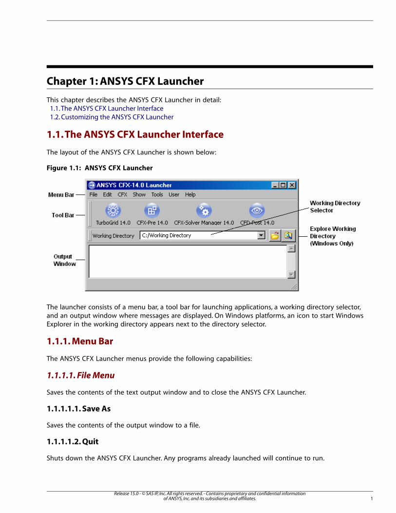
Chapter 1: ANSYS CFX Launcher
This chapter describes the ANSYS CFX Launcher in detail:1.1.The ANSYS CFX Launcher Interface1.2. Customizing the ANSYS CFX Launcher
1.1. The ANSYS CFX Launcher Interface
The layout of the ANSYS CFX Launcher is shown below:
Figure 1.1: ANSYS CFX Launcher
The launcher consists of a menu bar, a tool bar for launching applications, a working directory selector,and an output window where messages are displayed. On Windows platforms, an icon to start WindowsExplorer in the working directory appears next to the directory selector.
1.1.1. Menu Bar
The ANSYS CFX Launcher menus provide the following capabilities:
1.1.1.1. File Menu
Saves the contents of the text output window and to close the ANSYS CFX Launcher.
1.1.1.1.1. Save As
Saves the contents of the output window to a file.
1.1.1.1.2. Quit
Shuts down the ANSYS CFX Launcher. Any programs already launched will continue to run.
1Release 15.0 - © SAS IP, Inc. All rights reserved. - Contains proprietary and confidential information
of ANSYS, Inc. and its subsidiaries and affiliates.
1.1.1.2. Edit Menu
Clears the text output window, finds text in the text output window and sets options for the ANSYSCFX Launcher.
1.1.1.2.1. Clear
Clears the output window.
1.1.1.2.2. Find
Displays a dialog box where you can search the text in the output window.
1.1.1.2.3. Options
Presents the Options dialog box, which enables you to change the appearance of the ANSYS CFXLauncher.
1.1.1.2.3.1. User Interface Style
You can choose any one of several user interface styles; each style is available on all platforms. For ex-ample, choosing Windows will change the look and feel of the user interface to resemble that of aWindows application. You can select from Windows, Motif, CDE (Solaris), Plastique, and Cleanlooks styles.Once you have selected a style, click Apply to test.
1.1.1.2.3.2. Application Font and Text Window Font
The button to the right of Application Font sets the font used anywhere outside the text output window.The button to the right of Text Window Font applies only to the text output window. Clicking eitherof these buttons opens the Select Font dialog box.
1.1.1.3. CFX Menu
Enables you to launch CFX-Pre, CFX-Solver Manager, CFD-Post, and, if they are installed, other CFXproducts (such as ANSYS TurboGrid).
1.1.1.3.1. CFX-Pre
Runs CFX-Pre, with the working directory as specified in Working Directory Selector (p. 4).
1.1.1.3.2. CFX-Solver Manager
Runs CFX-Solver Manager, with the working directory as specified in Working Directory Selector (p. 4).
1.1.1.3.3. CFD-Post
Runs CFD-Post, in the current working directory as specified in Working Directory Selector (p. 4).
1.1.1.3.4. Other CFX Applications
The ANSYS CFX Launcher also searches for other CFX applications (for example, ANSYS TurboGrid) andprovides a menu entry to launch the application. If an application is not found, you can add it; for details,see Customizing the ANSYS CFX Launcher (p. 5).
Release 15.0 - © SAS IP, Inc. All rights reserved. - Contains proprietary and confidential informationof ANSYS, Inc. and its subsidiaries and affiliates.2
ANSYS CFX Launcher
1.1.1.4. Show Menu
Enables you to show system, installation, and other information.
1.1.1.4.1. Show Installation
Displays information about the version of CFX that you are running.
1.1.1.4.2. Show All
Displays all of the available information, including information about your system, installation, andvariables.
1.1.1.4.3. Show System
Displays information about the CFX installation and the system on which it is being run.
1.1.1.4.4. Show Variables
Displays the values of all the environment variables that are used in CFX.
1.1.1.5. Tools Menu
Enables you to access license-management tools and a command line for running other CFX utilities.
1.1.1.5.1. ANSYS Client Licensing Utility
Enables you to configure connections to ANSYS License Managers.
1.1.1.5.2. Command Line
Starts a command window from which you can run any of the CFX commands via the command lineinterface. The command line will be set up to run the correct version of CFX and the commands willbe run in the current working directory.
If you do not use the Tools > Command Line command to open a command window, then you willhave to either type the full path of the executable in each command, or explicitly set your operatingsystem path to include the <CFXROOT>/bin directory.
You may want to start components of CFX from the command line rather than by clicking the appropriatebutton on the ANSYS CFX Launcher for the following reasons:
• CFX contains some utilities (for example, a parameter editor) that can be run only from the commandline.
• You may want to specify certain command line arguments when starting up a component so that it startsup in a particular configuration.
• If you are having problems with a component, you may be able to get a more detailed error message bystarting the component from the command line than you would get if you started the component fromthe launcher. If you start a component from the command line, any error messages produced are writtento the command line window.
3Release 15.0 - © SAS IP, Inc. All rights reserved. - Contains proprietary and confidential information
of ANSYS, Inc. and its subsidiaries and affiliates.
The ANSYS CFX Launcher Interface
1.1.1.5.3. Configure User Startup Files (Linux only)
Information about creating startup files can be found in the installation documentation.
1.1.1.5.4. Edit File
Opens a browser to edit the text file of your choice in a platform-native text editor. Which text editoris called is controlled by the settings in <CFXROOT>/etc/launcher/shared.ccl .
1.1.1.5.5. Edit Site-wide Configuration File
Opens the site-wide configuration file in a text editor. Which text editor is called is controlled by thesettings in <CFXROOT>/etc/launcher/CFX5.ccl .
1.1.1.6. User Menu
The User menu is provided as an example. You can add your own applications to this menu, or createnew menus; for details, see Customizing the ANSYS CFX Launcher (p. 5).
1.1.1.7. Help Menu
The Help menu has the following commands:
CFX-Launcher
Opens CFX-Launcher help (this chapter), which describes the launcher interface as well as how to cus-tomize the launcher to, for example, add a menu entry that runs your own application.
CFX
You can select various topics including Contents, which will open up help documentation that describesthe CFX documentation set, Tutorials, and several topics.
About CFX-Launcher
This gives the point releases and software patches that are installed.
Help on Help
Opens documentation about the help system: Help On Help
Guidance on accessing CFX documentation is provided in Accessing Help.
1.1.2. Tool Bar
The toolbar contains shortcuts to the main components of CFX, for example CFX-Pre, CFX-Solver Managerand CFD-Post. Pressing any of the buttons will start up the component in the specified working directory.The equivalent menu entries for launching the components also show a keyboard shortcut that can beused to launch the component.
1.1.3. Working Directory Selector
While running CFX, all the files that are created will be stored in the working directory. To change theworking directory, you can do any of the following:
• Type the directory name into the box and press Enter.
• Click the down-arrow icon ( ) next to the directory name. This displays a list of recently used directories.
Release 15.0 - © SAS IP, Inc. All rights reserved. - Contains proprietary and confidential informationof ANSYS, Inc. and its subsidiaries and affiliates.4
ANSYS CFX Launcher
• Click Browse to browse to the directory that you want.
1.1.4. Output Window
The output window is used to display information from commands in the Show menu. You can right-click in the output window to show a shortcut menu with the following options:
• Find: Displays a dialog box where you can enter text to search for in the output.
• Select All: Selects all the text.
• Copy Selection: Copies the selected text.
• Save As: Saves the output to a file.
• Clear: Clears the output window.
1.2. Customizing the ANSYS CFX Launcher
Many parts of the ANSYS CFX Launcher are driven by CCL commands contained in configuration files.Some parts of the launcher are not editable (such as the File, Edit and Help menus), but others partsenable you to edit existing actions and create new ones (for example, launching your own applicationfrom the User menu). The following sections outline the steps required to configure the launcher. Theconfiguration files are located in the <CFXROOT>/etc/launcher/ directory (where <CFXROOT> isthe path to your installation of CFX). You can open these files in any text editor, but you should notedit any of the configuration files provided by CFX, other than the User.ccl configuration file.
1.2.1. CCL Structure
The configuration files contain CCL objects that control the appearance and behavior of menus andbuttons that appear in the ANSYS CFX Launcher. There are three types of CCL objects: GROUP, APPLICATION and DIVIDER objects. The fact that there are multiple configuration files is not important; ap-plications in one file can refer to groups in other files.
An example of how to add a menu item for the Windows calculator to the launcher is given in Example:Adding the Windows Calculator (p. 8).
1.2.1.1. GROUP
GROUP objects represent menus and toolbar groups in the ANSYS CFX Launcher. Each new GROUPcreates a new menu and toolbar. Nothing will appear in the menu or toolbar until you add APPLICATION or DIVIDER objects to the group. An example of a GROUP object is given below:
GROUP: CFX Position = 200 Menu Name = &CFX Show In Toolbar = Yes Show In Menu = Yes Enabled = YesEND
• The group name is set after the colon. In this case, it is "CFX". This is the name that APPLICATION andDIVIDER objects will refer to when you want to add them to this group. This name should be differentto all other GROUP objects.
5Release 15.0 - © SAS IP, Inc. All rights reserved. - Contains proprietary and confidential information
of ANSYS, Inc. and its subsidiaries and affiliates.
Customizing the ANSYS CFX Launcher
• Position refers to the position of the menu relative to others. The value should be an integer between1 and 1000. Groups with a higher Position value, relative to other groups, will have their menu appearfurther to the right in the menu bar. Referring to Figure 1.1: ANSYS CFX Launcher (p. 1), CFX has a lowerposition value than the ANSYS group. The File and Edit menus are always the first two menus and theHelp menu is always the last menu.
• The title of the menu is set under Menu Name (this menu has the title CFX). The optional ampersand isplaced before the letter that you want to have act as a menu accelerator (for example, Alt+C displays theCFX menu). You must be careful not to use an existing menu accelerator.
• The creation of the menu or toolbar can be toggled by setting the Show in Menu and Show inToolbar options to Yes or No respectively. For example, you may want to create a menu item but notan associated toolbar icon.
• Enabled sets whether the menu/toolbar is available for selection or is disabled. Set the option to No todisable it.
1.2.1.2. APPLICATION
APPLICATION objects create entries in the menus and toolbars that will launch an application or runa process. Two examples are given below with an explanation for each parameter. The first examplecreates a menu entry in the Tools menu that opens a command line window. The second examplecreates a menu entry and toolbar button to start CFX-Solver Manager.
APPLICATION: Command Line 1 Position = 300 Group = Tools Tool Tip = Start a window in which CFX commands can be run Menu Item Name = Command Line Command = <windir>\system32\cmd.exe Arguments = /c start Show In Toolbar = No Show In Menu = Yes Enabled = Yes OS List = winntENDAPPLICATION: CFXSM Position = 300 Group = CFX Tool Tip = Launches ANSYS CFX-Solver Manager Menu Item Name = CFX-&Solver Manager Command = cfx5solve Show In Toolbar = Yes Show In Menu = Yes Enabled = Yes Toolbar Name = ANSYS CFX-Solver Manager Icon = LaunchSolveIcon.xpm Shortcut = CTRL+SEND
• The application name is set after the colon, in the first example it is "Command Line 1 ". This nameshould be different from all other APPLICATION objects.
• Position : sets the relative position of the menu entry. The value should be an integer between 1 and1000. The higher the value, relative to other applications that have the same group, the further down themenu or the further to the right in a toolbar the entry will appear. If you do not specify a position, theobject assumes a high position value (so it will appear at the bottom of a menu or at the right of a groupof buttons).
Release 15.0 - © SAS IP, Inc. All rights reserved. - Contains proprietary and confidential informationof ANSYS, Inc. and its subsidiaries and affiliates.6
ANSYS CFX Launcher
• Group : sets the GROUP object to which this application belongs. The value must correspond to the namethat appears after "GROUP:" in an existing GROUP object. The menu and/or toolbar entry will not be createdif you do not specify a valid group name. The GROUP object does not have to be in the same configurationfile.
• Tool Tip : displays a message when the mouse pointer is held over a toolbar button. In the "CommandLine 1" example above, the Tool Tip entry is not used because a toolbar button is not created. Thisparameter is optional.
• Menu Item Name : sets the name of the entry that will appear in the menu. If you do not specify aname, the name is set to the name of the APPLICATION: object. The optional ampersand is placed beforethe letter that you want to have act as a menu accelerator (for example, Alt+C then S will start CFX-Solver Manager. Alt+C selects the CFX menu and S selects the entry from the menu). You must be carefulnot to use an existing menu accelerator.
• Command: contains the command to run the application. The path can be absolute (that is, use a forwardslash to begin the path on Linux, or a drive letter on Windows). If an absolute path is not specified, a rel-ative path from <CFXROOT>/bin/ is assumed. If no command is specified, the menu item/toolbar buttonwill not appear in the ANSYS CFX Launcher. The path and command are checked when the launcher isstarted. If the path or command does not exist, the menu item/toolbar button will not appear in thelauncher. You may find it useful to include environment variables in a command path; for details, see In-cluding Environment Variables (p. 8).
• Arguments : specifies any arguments that need to be passed to the application. The arguments are ap-pended to the value you entered for Command. You do not need to include this parameter as there areno arguments to pass. You may find it useful to include environment variables in the arguments; for details,see Including Environment Variables (p. 8).
Distinct arguments are space-separated. If you need to pass an argument that contains spaces (forexample, a Windows file path) you should include that argument in double quotes, for example:
Arguments = “ C:\Documents and Settings\User ” arg2 arg3
• Show In Toolbar : determines if a toolbar button is created for the application. This optional parameterhas a default value of Yes.
• Show In Menu : determines if a menu entry is created for the application. This optional parameter hasa default value of Yes .
• Enabled : controls the menu entry and toolbar button. Set this parameter to No to disable the application.This optional parameter has a default value of Yes .
• OS List is an optional parameter that enables you to set which operating system the application issuitable for. If OS List is not supplied, the launcher will attempt to create the menu item and toolbarbutton on all platforms.
For example, the command to open a command line window varies depending on the operatingsystem. In the ‘Command Line 1’ example above, the application only applies to Windows platforms.To complete the OS coverage, the launcher configuration files contain more ‘Command Line’ applic-ations that apply to different operating systems.
• Toolbar Name : sets the name that appears on the toolbar button. This parameter is optional (becauseyou may want to show only an icon).
7Release 15.0 - © SAS IP, Inc. All rights reserved. - Contains proprietary and confidential information
of ANSYS, Inc. and its subsidiaries and affiliates.
Customizing the ANSYS CFX Launcher
• Icon : specifies the icon to use on the toolbar button and in the menu item. The path can be absolute(that is, use a forward slash to begin the path on Linux, or a drive letter on Windows). If an absolute pathis not specified, a relative path from <CFXROOT>/etc/icons is assumed. The following file formats aresupported for icon image files: Portable Network Graphics (png ), Pixel Maps (ppm, xpm) and Bitmaps(bmp). Other icons used in the launcher are 32 pixels wide and 30 pixels high. This parameter is optional.If it is not included, an icon will not appear.
• Shortcut : specifies the keyboard shortcut that can be pressed to launch the application. You must becareful not to use a keyboard shortcut that is used by any other APPLICATION object.
1.2.1.2.1. Including Environment Variables
In can be useful to use environment variables in the values for some parameters. You can specify anenvironment variable value in any parameter by including its name between the < > symbols. In the‘Command Line 1’ example above, <windir> is used in the Command parameter so that the commandwould work on different versions of Windows. <windir> is replaced with the value held by the windirenvironment variable. The Command and Argument parameters are the only parameters that are likelyto benefit from using environment variables. Environment variables included in the Arguments para-meter are expanded before they are passed to the application.
1.2.1.3. DIVIDER
DIVIDER objects create a divider in a menu and/or toolbar (see the Tools menu for an example). Anexample of the CCL for DIVIDER objects is shown below.
DIVIDER: Tools Divider 1 Position = 250 Group = Tools OS List = winntEND
The Position , Group and OS List parameters are the same as those used in APPLICATION objects.For details, see APPLICATION (p. 6).
1.2.2. Example: Adding the Windows Calculator
The following CCL is the minimum required to add the Windows calculator to the ANSYS CFX Launcher:
GROUP: Windows Apps Menu Name = WindowsENDAPPLICATION: Calc Group = Windows Apps Command = <windir>\system32\calc.exe Toolbar Name = CalcEND
Although the parameter Toolbar Name is not strictly required, you would end up with a blank toolbarbutton if it were not set.
Release 15.0 - © SAS IP, Inc. All rights reserved. - Contains proprietary and confidential informationof ANSYS, Inc. and its subsidiaries and affiliates.8
ANSYS CFX Launcher
Chapter 2: Volume Mesh Import API
The Mesh Import Application Programming Interface (API) enables you to build a customized executablethat reads a 3-dimensional mesh from a 3rd-party mesh file into CFX-Pre and to extend the number offile formats that CFX-Pre can understand and read beyond those supplied as part of the standard install-ation.
The communication between the executable and CFX-Pre is via a communications channel that is con-trolled by use of routines in the API provided.
For details on using the Volume Mesh Import API, see User Import.
This chapter describes:2.1.Valid Mesh Elements in CFX2.2. Creating a Custom Mesh Import Executable for CFX-Pre2.3. Details of the Mesh Import API2.4. An Example of a Customized C Program for Importing Meshes into CFX-Pre2.5. Import Programs
2.1. Valid Mesh Elements in CFX
The CFX-Solver technology works with unstructured meshes. This does not prohibit the use of structuredmeshes. However a structured mesh will always be dealt with internally as an unstructured mesh.
The CFX-Solver can solve flows in any mesh comprising one or more of the following element types:
9Release 15.0 - © SAS IP, Inc. All rights reserved. - Contains proprietary and confidential information
of ANSYS, Inc. and its subsidiaries and affiliates.
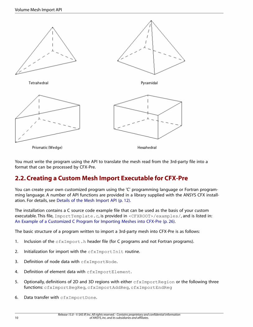
You must write the program using the API to translate the mesh read from the 3rd-party file into aformat that can be processed by CFX-Pre.
2.2. Creating a Custom Mesh Import Executable for CFX-Pre
You can create your own customized program using the 'C' programming language or Fortran program-ming language. A number of API functions are provided in a library supplied with the ANSYS CFX install-ation. For details, see Details of the Mesh Import API (p. 12).
The installation contains a C source code example file that can be used as the basis of your customexecutable. This file, ImportTemplate.c , is provided in <CFXROOT>/examples/ , and is listed in:An Example of a Customized C Program for Importing Meshes into CFX-Pre (p. 26).
The basic structure of a program written to import a 3rd-party mesh into CFX-Pre is as follows:
1. Inclusion of the cfxImport.h header file (for C programs and not Fortran programs).
2. Initialization for import with the cfxImportInit routine.
3. Definition of node data with cfxImportNode .
4. Definition of element data with cfxImportElement .
5. Optionally, definitions of 2D and 3D regions with either cfxImportRegion or the following threefunctions: cfxImportBegReg , cfxImportAddReg , cfxImportEndReg
6. Data transfer with cfxImportDone .
Release 15.0 - © SAS IP, Inc. All rights reserved. - Contains proprietary and confidential informationof ANSYS, Inc. and its subsidiaries and affiliates.10
Volume Mesh Import API
The header files associated with the API are located in <CFXROOT>/include/ . If you do not use theheader file cfxImport.h , the functionality of the routines contained within the API may not followdefined behavior.
After writing the program, you will need to compile the source code. For details, see Compiling Codewith the Mesh Import API (p. 11).
You will also need to link your routine with the API routine libraries. For details, see Linking Code withthe Mesh Import API (p. 11).
After a customized executable has been produced, it can be run in CFX-Pre. For details, see User Import.
2.2.1. Compiling Code with the Mesh Import API
Compilation of a customized executable must be performed using an appropriate compiler and compilerflags.
The customized executable must also be linked with the provided mesh import API library and theprovided I/O library as detailed in Linking Code with the Mesh Import API (p. 11).
Note
Windows users should note that custom mesh import programs must be compiled as multi-threaded applications.
2.2.2. Linking Code with the Mesh Import API
In order to build a customized import utility routine, it must be linked with several libraries. These lib-raries are located in <CFXROOT>/lib/< os>/ :
• libmeshimport.lib (on Windows), or libmeshimport.a (on Linux)
• libratlas_api.lib (on Windows), or libratlas_api.a (on Linux)
• libratlas.lib (on Windows), or libratlas.a (on Linux)
• libpgtapi.lib (on Windows), or libpgtapi.a (on Linux)
• libunits.lib (on Windows), or libunits.a (on Linux)
• libcclapilt.lib (on Windows), or libcclapilt.a (on Linux)
• libio.lib (on Windows), or libio.a (on Linux)
2.2.2.1. Linking a Customized C Mesh Import Executable on a UNIX Platform
On most UNIX systems you should be able to build the executable with the command:
cc myimport.c -I<CFXROOT>/include/ -o myimport -L<CFXROOT>/lib/< os> \ -lmeshimport -lratlas_api -lratlas -lpgtapi -lunits -lcclapilt -lio \ -lm -lc
Here, -lmeshimport , -lratlas_api , -lratlas , -lpgtapi , -lunits , -lcclapillt , and -lioindicate the libraries mentioned above, while -lm and -lc are system libraries.
11Release 15.0 - © SAS IP, Inc. All rights reserved. - Contains proprietary and confidential information
of ANSYS, Inc. and its subsidiaries and affiliates.
Creating a Custom Mesh Import Executable for CFX-Pre
In this example, your own import program is named myimport.c and the executable file will be calledmyimport . You should ensure that the libraries to which you are linking (which are in the path givenafter -L ) appear on the command line after the source file (or object file if you are just linking to anexisting object).
You can use the GCC compiler v4.6.1 with ANSYS CFX 15.0.
2.2.2.2. Linking a Customized Fortran Mesh Import Executable on a UNIX Platform
The following is an example of how to build the executable on Linux, when the source code for theexecutable is written in Fortran:
pgf95 myimport.F -L< CFXROOT>/lib/linux-amd64 -lmeshimport -lratlas_api -lratlas \ -lpgtapi -lunits -lcclapilt -lio -lm -o myimport.exe
Note
The officially supported pgf compiler is required.
2.2.2.3. Linking a Customized Mesh Import Executable on a 32-bit Windows Platform
You can build the executables on 32-bit Windows systems that have the C++ compiler of MicrosoftVisual Studio 2010. An example command line follows:
cl /MD /I "C:\Program Files\Ansys Inc\v150\CFX\include" ImportTemplate.c/link /libpath:"C:\Program Files\Ansys Inc\v150\CFX\lib\winnt" lib-cclapilt.lib libio.lib libmeshimport.lib libunits.lib libpgtapi.lib lib-ratlas_api.lib libratlas.lib
2.2.2.4. Linking a Customized Mesh Import Executable on a 64-bit Windows Platform
You can build the executables on 64-bit Windows systems that have the C++ compiler of MicrosoftVisual Studio 2010. An example command line follows:
cl /MD /I "C:\Program Files\Ansys Inc\v150\CFX\include" ImportTemplate.c/link /libpath:"C:\Program Files\Ansys Inc\v150\CFX\lib\winnt-amd64"libcclapilt.lib libio.lib libmeshimport.lib libunits.lib libpgtapi.liblibratlas_api.lib libratlas.lib
2.3. Details of the Mesh Import API
This section contains information about the functions that are used to write a customized import ex-ecutable in the Mesh Import API.
Before trying to use any of the routines listed in this section, it is highly recommended that you readCreating a Custom Mesh Import Executable for CFX-Pre (p. 10).
This section contains details of:
• Defined Constants (p. 13)
• Initialization Routines (p. 14)
• Termination Routines (p. 15)
Release 15.0 - © SAS IP, Inc. All rights reserved. - Contains proprietary and confidential informationof ANSYS, Inc. and its subsidiaries and affiliates.12
Volume Mesh Import API
• Error Handling Routines (p. 15)
• Node Routines (p. 16)
• Element Routines (p. 16)
• Primitive Region Routines (p. 19)
• Composite Regions Routines (p. 21)
• Explicit Node Pairing (p. 21)
• Fortran Interface (p. 22)
• Unsupported Routines Previously Available in the API (p. 25)
Note
In past releases of ANSYS CFX the API has defined IDs of nodes and elements as integers(int). This release now uses a datatype ID_t to represent these quantities. This type is currentlydefined as an unsigned integer (unsigned int). This allows a greater number of nodes andelements to be imported than in the past.
2.3.1. Defined Constants
The following are defined in the header file cfxImport.h , which should be included in the importprogram.
2.3.1.1. Element Types
There are currently 4 types of elements, which are identified by the number of nodes: Tetrahedrons (4nodes), pyramids (5 nodes), wedges or prisms (6 nodes), and hexahedrons (8 nodes). The element typesmay be identified by the defined constants:
#define cfxELEM_TET 4#define cfxELEM_PYR 5#define cfxELEM_WDG 6#define cfxELEM_HEX 8
The element node ordering and local face numbering follow Patran Neutral file conventions for elementdescriptions.
2.3.1.2. Region Types
Regions may be defined in terms of nodes, faces or elements, based on the type argument to thecfxImportBegReg or cfxImportRegion routines. The three types are defined by the definedconstants:
#define cfxImpREG_NODES 1#define cfxImpREG_FACES 2#define cfxImpREG_ELEMS 3
Node and Face regions define 2D regions of the imported mesh. Element regions define 3D regions ofthe imported mesh.
13Release 15.0 - © SAS IP, Inc. All rights reserved. - Contains proprietary and confidential information
of ANSYS, Inc. and its subsidiaries and affiliates.
Details of the Mesh Import API

It is best to use face regions to define 2D regions of the mesh and element regions to define 3D regionsof the mesh.
Node regions will be automatically transformed into a face region by the import process. This transform-ation requires the node IDs specified to define vertices of valid element faces. If no element faces canbe constructed from the defined node region the node region will be deleted.
Note
Due to the limited topological information recoverable from a set of nodes it is not advisableto define 2D regions internal to a 3D region using nodes. In this case it is advisable to useFace regions.
Node regions are specified by a list of node IDs.
Face regions are defined by a list of face IDs. These face IDs are a combination of an element ID and alocal face number in the element.
2.3.2. Initialization Routines
The following routines check and initialize the Import API. With the exception of cfxImportStatusthe first call to the Import API must be either cfxImportInit for communication with CFX, or cfxImportTest for testing the import routine in stand-alone mode.
2.3.2.1. cfxImportStatus
int cfxImportStatus ()
Returns 0 if descriptor is not opened and -1 if not opened for writing. In the normal case, 1 is returnedif opened for writing to CFX, and 2 if opened for writing to a file.
2.3.2.2. cfxImportInit
void cfxImportInit ()
Performs initialization to begin communicating with CFX. This routine should be called early on in theimport program to let CFX know that data is to be sent. If not called within 60 seconds, CFX will terminatethe import process. If called and there is no connection with CFX, then the routine cfxImportTest("/dev/null") (UNIX) or cfxImportTest("null") (Windows) will be called. This routinewill be automatically called by most of the API routines if not already called.
There is no return value for this routine. In the case of an error, cfxImportFatal will be called.
2.3.2.3. cfxImportTest
int cfxImportTest (filename) char *filename;
This routine allows testing of import program in isolation from CFX by writing data to a file filenameinstead of attempting to write it to the CFX communication channel.
The routine will return the file descriptor of the output file or will terminate with a call to cfxImportFatal on error.
Release 15.0 - © SAS IP, Inc. All rights reserved. - Contains proprietary and confidential informationof ANSYS, Inc. and its subsidiaries and affiliates.14
Volume Mesh Import API
2.3.3. Termination Routines
With the exception of cfxImportTotals the last call to the Import API must always be cfxImportDone . This function performs the final processing of the import data, and then transfers the datato CFX.
2.3.3.1. cfxImportDone
long cfxImportDone ()
Indicate to the import API that all mesh data has been given and the API should now send the data toCFX. Except for cfxImportTotals , this should be last call made to the API. Returns the total numberof bytes transferred to CFX by the import program.
2.3.3.2. cfxImportTotals
long cfxImportTotals (counts)size_t counts[cfxImpCNT_SIZE];
Get the total number of nodes, elements, regions and other useful information given to the mesh importAPI by the program. This information is returned in the array counts , which should be of size at leastcfxImpCNT_SIZE (currently defined as 9). The values returned in counts may be indexed by theenum list in cfxImport.h , which is:
counts[cfxImpCNT_NODE] = number of nodescounts[cfxImpCNT_ELEMENT] = number of elementscounts[cfxImpCNT_REGION] = number of regionscounts[cfxImpCNT_UNUSED] = number of unused nodescounts[cfxImpCNT_DUP] = number of duplicate nodescounts[cfxImpCNT_TET] = number of tetrahedral elementscounts[cfxImpCNT_PYR] = number of pyramid elementscounts[cfxImpCNT_WDG] = number of wedge elementscounts[cfxImpCNT_HEX] = number of hexahedral elements
The return value for the function is the total number of bytes of data sent to CFX or written to the testfile given when cfxImportTest was called.
2.3.4. Error Handling Routines
The first error handling routine allows the programmer to define an error callback function that is calledwhen a fatal error is generated by the API or explicitly by the programmers code.
The second routine performs a method for clean termination of the program, shutting down the programand communication with ANSYS CFX.
2.3.4.1. cfxImportError
void cfxImportError (callback)void (*callback)(char *errmsg);
Define a user routine to be called before terminating due to a fatal error. callback is the application-supplied function to be called in the case of an error. The callback routine takes a single argument,errmsg , which will be passed by cfxImportFatal and should be processed by the callback functionas a brief message describing the error that has occurred. If this function is not called or callback is notspecified, then the normal termination behavior of the mesh import API will be that the any fatal errorswill write the error message to stderr as well as being sent to CFX.
15Release 15.0 - © SAS IP, Inc. All rights reserved. - Contains proprietary and confidential information
of ANSYS, Inc. and its subsidiaries and affiliates.
Details of the Mesh Import API
2.3.4.2. cfxImportFatal
void cfxImportFatal (errmsg)char *errmsg;
Terminate with an error message, errmsg . This routine will send the message to CFX, shut down thecommunication channel or test file and call the user callback function (if specified by a call to cfxImpor-tError).
There is no return from this call. The import program will terminate immediately after clean up taskshave been performed.
2.3.5. Node Routines
These routines define the 3D coordinates of points in space(nodes) that will be used to define elementsor 2D regions that are to be imported to CFX. Each node has a unique identifier called a node ID.
2.3.5.1. cfxImportNode
ID_t cfxImportNode (nodeid, x, y, z)ID_t nodeid;double x, y, z;
Define a node in the import API to be subsequently imported into CFX. The unique identifier of thenode is given by nodeid , and the coordinates of the node by x, y, and z.
Returns 0 if nodeid is invalid (less than 1), or nodeid is successfully defined. If a node with the sameidentity has already been defined, the coordinate values will alter to the supplied values.
2.3.5.2. cfxImportGetNode
ID_t cfxImportGetNode (nodeid, x, y, z)ID_t nodeid;double *x, *y, *z;
Get the coordinates for the node identified by nodeid and return the values in x , y , and z . Returns 0if the node has not been defined or the node ID for the node.
2.3.5.3. cfxImportNodeList
ID_t * cfxImportNodeList ()
Returns an array of all node identifiers currently defined or NULL if no nodes have been defined. Thefirst entry in the array is the number of nodes currently defined.
The memory for the array returned is allocated using malloc by the routine, consequently it shouldbe destroyed when no longer required by calling free .
2.3.6. Element Routines
The following routines define the topology of elements (using node IDs) that are to be imported toCFX. Also included here are routines that get the local face number and vertices of an element.
2.3.6.1. cfxImportElement
ID_t cfxImportElement (elemid, elemtype, nodelist)ID_t elemid, *nodelist; int elemtype;
Release 15.0 - © SAS IP, Inc. All rights reserved. - Contains proprietary and confidential informationof ANSYS, Inc. and its subsidiaries and affiliates.16
Volume Mesh Import API
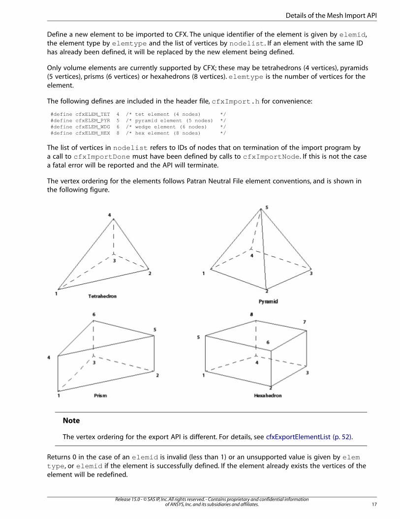
Define a new element to be imported to CFX. The unique identifier of the element is given by elemid ,the element type by elemtype and the list of vertices by nodelist . If an element with the same IDhas already been defined, it will be replaced by the new element being defined.
Only volume elements are currently supported by CFX; these may be tetrahedrons (4 vertices), pyramids(5 vertices), prisms (6 vertices) or hexahedrons (8 vertices). elemtype is the number of vertices for theelement.
The following defines are included in the header file, cfxImport.h for convenience:
#define cfxELEM_TET 4 /* tet element (4 nodes) */#define cfxELEM_PYR 5 /* pyramid element (5 nodes) */#define cfxELEM_WDG 6 /* wedge element (6 nodes) */#define cfxELEM_HEX 8 /* hex element (8 nodes) */
The list of vertices in nodelist refers to IDs of nodes that on termination of the import program bya call to cfxImportDone must have been defined by calls to cfxImportNode . If this is not the casea fatal error will be reported and the API will terminate.
The vertex ordering for the elements follows Patran Neutral File element conventions, and is shown inthe following figure.
Note
The vertex ordering for the export API is different. For details, see cfxExportElementList (p. 52).
Returns 0 in the case of an elemid is invalid (less than 1) or an unsupported value is given by elemtype , or elemid if the element is successfully defined. If the element already exists the vertices of theelement will be redefined.
17Release 15.0 - © SAS IP, Inc. All rights reserved. - Contains proprietary and confidential information
of ANSYS, Inc. and its subsidiaries and affiliates.
Details of the Mesh Import API
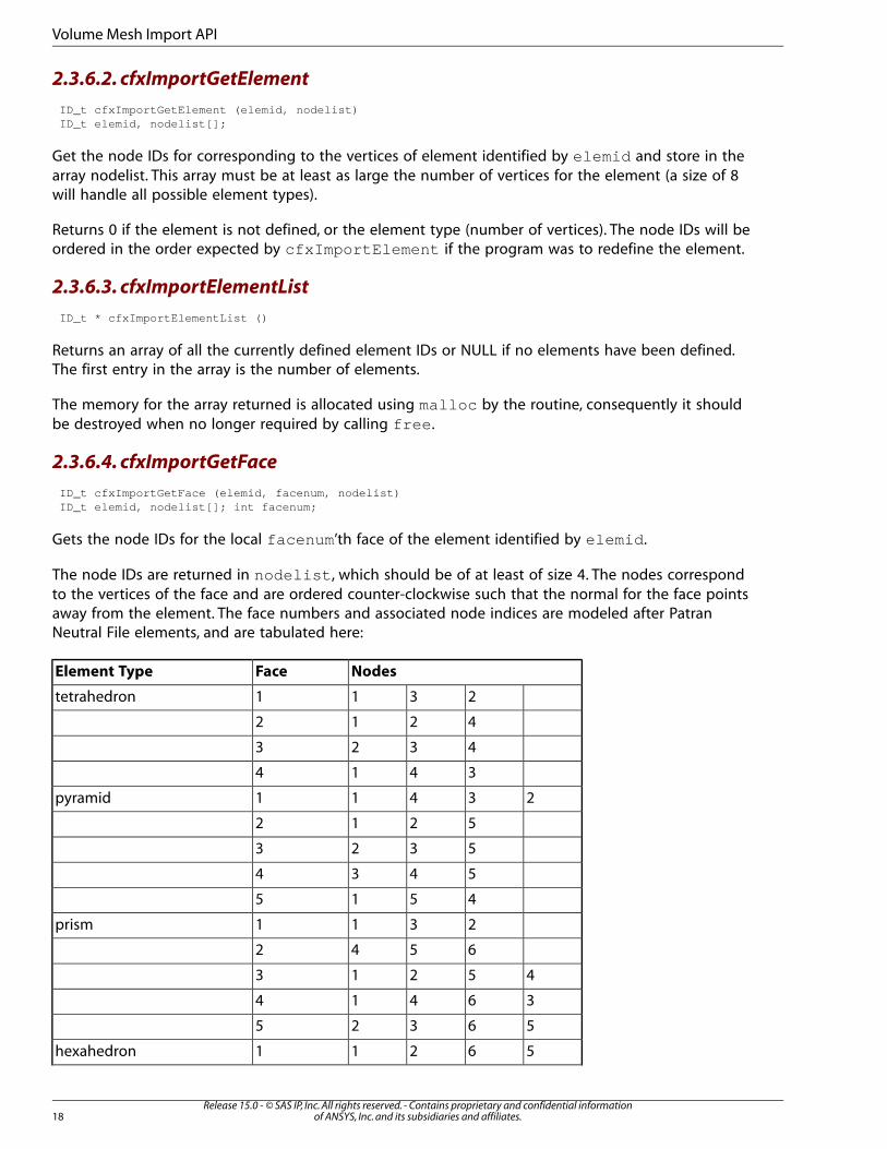
2.3.6.2. cfxImportGetElement
ID_t cfxImportGetElement (elemid, nodelist)ID_t elemid, nodelist[];
Get the node IDs for corresponding to the vertices of element identified by elemid and store in thearray nodelist. This array must be at least as large the number of vertices for the element (a size of 8will handle all possible element types).
Returns 0 if the element is not defined, or the element type (number of vertices). The node IDs will beordered in the order expected by cfxImportElement if the program was to redefine the element.
2.3.6.3. cfxImportElementList
ID_t * cfxImportElementList ()
Returns an array of all the currently defined element IDs or NULL if no elements have been defined.The first entry in the array is the number of elements.
The memory for the array returned is allocated using malloc by the routine, consequently it shouldbe destroyed when no longer required by calling free .
2.3.6.4. cfxImportGetFace
ID_t cfxImportGetFace (elemid, facenum, nodelist)ID_t elemid, nodelist[]; int facenum;
Gets the node IDs for the local facenum ’th face of the element identified by elemid .
The node IDs are returned in nodelist , which should be of at least of size 4. The nodes correspondto the vertices of the face and are ordered counter-clockwise such that the normal for the face pointsaway from the element. The face numbers and associated node indices are modeled after PatranNeutral File elements, and are tabulated here:
NodesFaceElement Type
2311tetrahedron
4212
4323
3414
23411pyramid
5212
5323
5434
4515
2311prism
6542
45213
36414
56325
56211hexahedron
Release 15.0 - © SAS IP, Inc. All rights reserved. - Contains proprietary and confidential informationof ANSYS, Inc. and its subsidiaries and affiliates.18
Volume Mesh Import API
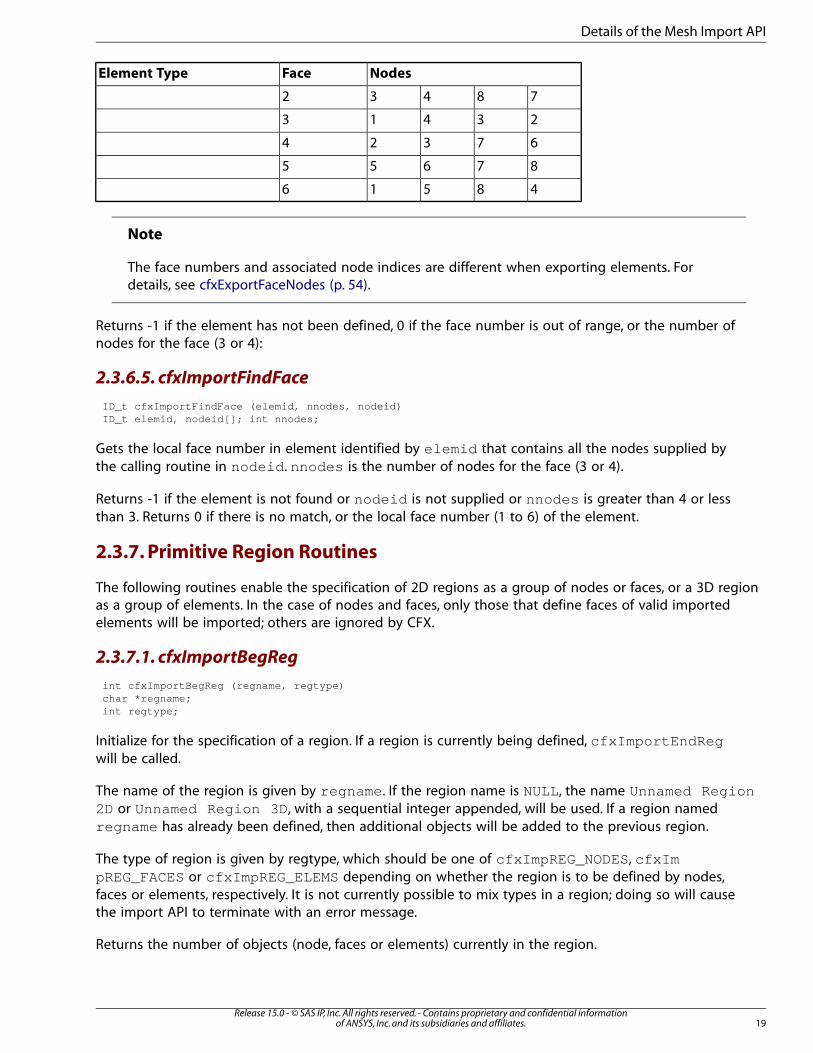
NodesFaceElement Type
78432
23413
67324
87655
48516
Note
The face numbers and associated node indices are different when exporting elements. Fordetails, see cfxExportFaceNodes (p. 54).
Returns -1 if the element has not been defined, 0 if the face number is out of range, or the number ofnodes for the face (3 or 4):
2.3.6.5. cfxImportFindFace
ID_t cfxImportFindFace (elemid, nnodes, nodeid)ID_t elemid, nodeid[]; int nnodes;
Gets the local face number in element identified by elemid that contains all the nodes supplied bythe calling routine in nodeid . nnodes is the number of nodes for the face (3 or 4).
Returns -1 if the element is not found or nodeid is not supplied or nnodes is greater than 4 or lessthan 3. Returns 0 if there is no match, or the local face number (1 to 6) of the element.
2.3.7. Primitive Region Routines
The following routines enable the specification of 2D regions as a group of nodes or faces, or a 3D regionas a group of elements. In the case of nodes and faces, only those that define faces of valid importedelements will be imported; others are ignored by CFX.
2.3.7.1. cfxImportBegReg
int cfxImportBegReg (regname, regtype)char *regname;int regtype;
Initialize for the specification of a region. If a region is currently being defined, cfxImportEndRegwill be called.
The name of the region is given by regname . If the region name is NULL, the name Unnamed Region2D or Unnamed Region 3D , with a sequential integer appended, will be used. If a region namedregname has already been defined, then additional objects will be added to the previous region.
The type of region is given by regtype, which should be one of cfxImpREG_NODES, cfxImpREG_FACES or cfxImpREG_ELEMS depending on whether the region is to be defined by nodes,faces or elements, respectively. It is not currently possible to mix types in a region; doing so will causethe import API to terminate with an error message.
Returns the number of objects (node, faces or elements) currently in the region.
19Release 15.0 - © SAS IP, Inc. All rights reserved. - Contains proprietary and confidential information
of ANSYS, Inc. and its subsidiaries and affiliates.
Details of the Mesh Import API
2.3.7.2. cfxImportAddReg
int cfxImportAddReg (numobjs, objlist)int numobjs, *objlist;
Add IDs of objects being defined to the current region.
A region must be currently defined or reactivated by cfxImportBegReg or an error will occur, andthe API will terminate.
The number of objects to add is given by numobjs and the IDs of the objects are supplied in objlist .
The objects are interpreted as node IDs, face IDs, or element IDs, depending on the type of the regionindicated when cfxImportBegReg was called.
On calling cfxImportDone , any node IDs , face IDs or element IDs specified in the object list musthave been defined by the appropriate routine or they will be removed from the region.
Returns the total number of objects in the current region after the object IDs have been added.
2.3.7.3. cfxImportEndReg
int cfxImportEndReg ()
End the specification of the current region.
Returns the number of objects (nodes, faces or elements) in the region.
2.3.7.4. cfxImportRegion
int cfxImportRegion (regname, regtype, numobjs, objlist)char *regname;int regtype, numobjs, *objlist;
Import a region named regname of type regtype . The number of objects to add to the region isgiven by numobjs , and the list of object IDs by objlist . This routine combines calls to cfxImportBegReg, cfxImportAddReg and cfxImportEndReg .
Returns the total number of objects in the region on termination of the routine.
2.3.7.5. cfxImportRegionList
char ** cfxImportRegionList ()
Return a NULL terminated list of currently defined region names.
The memory for the array and each character string in the array returned is allocated using mallocby the routine, consequently each array member and the array itself should be destroyed when nolonger required by calling free .
2.3.7.6. cfxImportGetRegion
int * cfxImportGetRegion (regname)char *regname;
Returns a list of objects in the region named regname , or NULL if the region does not exist. The firstentry in the returned list is the region type and the second entry is the number of object IDs.
Release 15.0 - © SAS IP, Inc. All rights reserved. - Contains proprietary and confidential informationof ANSYS, Inc. and its subsidiaries and affiliates.20
Volume Mesh Import API
The memory for the array is allocated using malloc by the routine, consequently the array itself shouldbe destroyed when no longer required by calling free .
2.3.8. Composite Regions Routines
The following routines enable composite regions to be defined in terms of primitive regions or othercomposite regions.
2.3.8.1. cfxImportBegCompRegion
cfxImportBegCompReg()char *regionName;
Begin defining a composite region with the name regionName ,
Returns -1 if a primitive region regionName is already defined or memory couldn’t be allocated, or 0if successfully created.
2.3.8.2. cfxImportAddCompRegComponents
int cfxImportAddCompRegComponents(componentCount,components)int componentCount;char **components;
Add a set of component region names specified in components to the composite region currentlybeing defined. componentCount specified how many components are specified in the componentsarray,
Returns -1 if a composite region is not being defined or insufficient memory is available to add thecomponents of the composite region, or 0 if the components were successfully added.
2.3.8.3. cfxImportEndCompReg
int cfxImportEndCompReg()
Finish defining the current composite region.
Returns -1 if a composite region is not currently being defined or 0 otherwise.
2.3.8.4. cfxImportCompositeRegion
int cfxImportCompositeRegion(regionName, componentCount, components)char *regionName, **components;int componentCount;
Define a composite region named regionName with componentCount components supplied incharacter array components .
Returns 0 if successful or -1 if an error occurred preventing the composite region being defined.
2.3.9. Explicit Node Pairing
The following routine provides a method for explicitly marking two nodes as being identical (or in thesame position in space).
21Release 15.0 - © SAS IP, Inc. All rights reserved. - Contains proprietary and confidential information
of ANSYS, Inc. and its subsidiaries and affiliates.
Details of the Mesh Import API
2.3.9.1. cfxImportMap
ID_t cfxImportMap (nodeid, mapid)ID_t nodeid, mapid;
Explicitly map the node identified by nodeid to the node identified by mapid .
On calling cfxImportDone the Mesh Import API will update regions and elements referencing themapped node to the node it is mapped to. This therefore reduces the total node count imported toCFX and eliminates the duplicate nodes.
Duplicate nodes may also be removed by CFX if the appropriate options are selected in the CFX interfaceand an appropriate tolerance set. For details, see Importing Meshes in the CFX-Pre User's Guide.
2.3.10. Fortran Interface
The following routines are callable from Fortran, and interface with the corresponding C routine. Thereare currently no return values.
2.3.10.1. cfxinit
call cfxinit
Interface to cfxImportInit . Initializes for import.
2.3.10.2. cfxtest
CHARACTER*n filenamecall cfxtest(filename)
Interface to cfxImportTest . filename is a CHARACTER*n value that gives the name of the file todump the output to.
2.3.10.3. cfxunit
CHARACTER*n unitscall cfxunit(units)
Interface to cfxImportUnits . Specify the units the mesh is specified in.
2.3.10.4. cfxwarn
CHARACTER*n mesgcall cfxwarn(mesg)
Interface to cfxImportWarning . Emit a warning message mesg.
2.3.10.5. cfxfatl
CHARACTER*n mesgcall cfxfatl(mesg)
Interface to cfxImportFatal . Emit a warning message mesg and terminate the program cleanly.
2.3.10.6. cfxdone
call cfxdone
Interface to cfxImportDone . Terminates the program and transfers the data to CFX-Pre.
Release 15.0 - © SAS IP, Inc. All rights reserved. - Contains proprietary and confidential informationof ANSYS, Inc. and its subsidiaries and affiliates.22
Volume Mesh Import API
2.3.10.7. cfxnode
INTEGER idnodeDOUBLE PRECISION x,y,zcall cfxnode(idnode,x,y,z)
Interface to cfxImportNode . Imports a node with the specified coordinates. idnode is an INTEGERvalue for the node ID, and x, y, and z are the DOUBLE PRECISION coordinates of the node.
2.3.10.8. cfxnodg
INTEGER idnodeDOUBLE PRECISION x,y,zcall cfxnodg(idnode,x,y,z)
Interface to cfxImportGetNode . Queries the current coordinates or a node referenced by idnode .idnode is an INTEGER value for the node ID, and x, y, and z are the DOUBLE PRECISION coordinatesof the node.
2.3.10.9. cfxnods
INTEGER ids(*)call cfxnods(ids)
Interface to cfxImportNodeList . Retrieves the list of all valid node IDs having been imported intothe API. ids is an INTEGER array that must be at least as large as the number of nodes currently imported.
2.3.10.10. cfxelem
INTEGER idelem,itelem,nodes(*)call cfxelem(idelem,itelem,nodes)
Interface to cfxImportElement . idelem is element ID, and itelem is the element type (numberof nodes - 4,5,6, or 8). Both are of type INTEGER. nodes is an array of INTEGER node IDs dimensionedof size at least itelem .
2.3.10.11. cfxeleg
INTEGER idelem,itelem,nodes(*)call cfxeleg(idelem,itelem,nodes)
Interface to cfxImportGetElement . Queries the current node ids that define the vertices of theelement referenced by the id idelem . idelem is element ID, and itelem is the element type (numberof nodes - 4, 5, 6, or 8). Both are of type INTEGER. nodes is an array of INTEGER values that will containthe node IDs on successful return. It should be dimensioned of size at least itelem .
2.3.10.12. cfxeles
INTEGER ids(*)call cfxeles(ids)
Interface to cfxImportElemList . Retrieves the list of all valid element IDs having been importedinto the API. ids is an INTEGER array that must be at least as large as the number of elements currentlyimported.
2.3.10.13. cfxfacd
INTEGER eleid, elefc, idcall cfxfacd(eleid, elefc, id)
23Release 15.0 - © SAS IP, Inc. All rights reserved. - Contains proprietary and confidential information
of ANSYS, Inc. and its subsidiaries and affiliates.
Details of the Mesh Import API
Interface to cfxImportFaceID . Defines a face id (id ) in terms of an element ID (eleid ) and localface (elefc ) of that element.
2.3.10.14. cfxface
INTEGER eleid, elefc, vtx(*)INTEGER cfxface(eleid, elefc, vtx)
Interface to cfxImportGetFace . Returns the node IDs of the vertices defining a face located by theelement ID (eleid ) and local face (elefc ) of that element.
2.3.10.15. cfxffac
INTEGER eleid, nvtx, vtx(*), elefccall cfxffac(eleid, nvtx, vtx, elefc)
Interface to cfxImportFindFace . Returns the local face (elefc ) of an element (eleid ) that isdefined by the vertices (vtx ).
2.3.10.16. cfxregn
CHARACTER*n regnameINTEGER type,nobjs,objs(*)call cfxregn(regname,type,nobjs,objs)
Interface to cfxImportRegion . Regname is a CHARACTER*n string defining the region name, typeis an INTEGER value specifying the type of region, either 1 for nodes, 2 for faces, or 3 for elements.nobjs is an INTEGER value that gives the number of objects in the region, and objs is an INTEGER arrayof object IDs dimensioned at least size nobjs .
2.3.10.17. cfxregb
CHARACTER*n regnameINTEGER typecall cfxregb(regname,type)
Interface to cfxImportBegReg . Start defining a new region or make an existing region of the samename the current one if it already exists and is of the same type. regname is a CHARACTER*n stringdefining the region name, type is an INTEGER value specifying the type of region, either 1 for nodes, 2for faces, or 3 for elements.
2.3.10.18. cfxrega
INTEGER nobjs,objs(*)call cfxrega(nobjs,objs)
Interface to cfxImportAddReg . Add the objects (objs ) to the current region. nobjs is an INTEGERvalue that gives the number of objects to add to the region, and objs is an INTEGER array of objectIDs dimensioned at least size nobjs .
2.3.10.19. cfxrege
call cfxrege()
Interface to cfxImportEndReg . Finish defining the current region (after the call there will be nocurrent region).
Release 15.0 - © SAS IP, Inc. All rights reserved. - Contains proprietary and confidential informationof ANSYS, Inc. and its subsidiaries and affiliates.24
Volume Mesh Import API
2.3.10.20. cfxregs
CHARACTER*n regnameINTEGER numobjcall cfxregs(regname,numobj)
Query how many objects (returned in numobj ) are referenced by the region regname . regname is aCHARACTER*n string specifying the region name.
2.3.10.21. cfxregg
CHARACTER*n regnameINTEGER type, obj(*)call cfxregg(regname, type, objs)
Get the type (type ) and object IDs (objs ) referenced by the region regname . regname is a CHARAC-TER*n string specifying the region name. type is INTEGER and objs is an INTEGER array at least of thesize returned by cfxregs .
2.3.10.22. cfxcmpb
CHARACTER*n regnamecall cfxcmpb(regname)
Interface to cfxImportBegCompReg . Start defining a new composite region or make an existingcomposite region of the same name as the current one if it already exists. regname is a CHARACTER*nstring defining the region name.
2.3.10.23. cfxcmpa
INTEGER nregsCHARACTER*(n) regscall cfxcmpa(nregs,regs)
Interface to cfxImportAddCompReg . Add the region names (regs ) to the current composite regionbeing defined. nregs is an INTEGER value that gives the number of regions to add to the region, andregs is a CHARACTER*(*) array of region names dimensioned at least size nregs .
2.3.10.24. cfxcmpe
call cfxcmpe()
Interface to cfxImportEndCompReg . Finish defining the current composite region (after the call therewill be no current composite region).
2.3.11. Unsupported Routines Previously Available in the API
In ANSYS CFX 15.0 certain functionality available in previous releases is no longer supported. Theseroutines have been removed because they are directly implemented in CFX.
The following is a list of routines removed from the mesh import API:
cfxImportFixElements cfxImportTolerancecfxImportGetTolcfxImportSetCheckcfxImportRangecfxImportCheckcfxtolcfxsetcfxchk
25Release 15.0 - © SAS IP, Inc. All rights reserved. - Contains proprietary and confidential information
of ANSYS, Inc. and its subsidiaries and affiliates.
Details of the Mesh Import API
2.4. An Example of a Customized C Program for Importing Meshes into
CFX-Pre
An example, ImportTemplate.c , can be found in <CFXROOT>/examples .
2.5. Import Programs
The following sections detail the standard import programs currently available within CFX-Pre and theircommand line equivalents.
Information about importing meshes from the CFX-Pre interface is given in Importing Meshes in theCFX-Pre User's Guide.
If you want to use command line options that cannot be specified through the CFX-Pre User Interface,then you may want to run these programs as user-defined mesh import programs. User Import detailshow to run a mesh import program.
The executables are located in <CFXROOT>/bin/< os>.
• ANSYS (p. 26)
• CFX Def/Res (p. 27)
• CFX-4 (p. 27)
• CFX-5.1 (p. 27)
• CFX-TfC (p. 29)
• CGNS (p. 29)
• Fluent (p. 30)
• GridPro/az3000 (p. 30)
• I-DEAS (p. 31)
• ICEM CFX (p. 31)
• PATRAN (p. 31)
• NASTRAN (p. 32)
• CFX-TASCflow (p. 32)
2.5.1. ANSYS
Imports an ANSYS file. The external import routine is ImportANSYS . Available options are:
-v Verbose output. Echo additional data to stdout during the import.
-E Import Elements of the same type as regions.
-A Import ANSA parts as regions.
Release 15.0 - © SAS IP, Inc. All rights reserved. - Contains proprietary and confidential informationof ANSYS, Inc. and its subsidiaries and affiliates.26
Volume Mesh Import API
-S Display a list of all supported element types.
2.5.2. CFX Def/Res
Imports the mesh from a CFX-Solver input or results file. The external import routine is ImportDef .Available options are:
-v Verbose output. Echo additional data to stdout during the import.
-I Read mesh from the initial timestep in the file.
-L Read mesh from the last timestep in the file.
-T< timestep> Read mesh from the timestep specified (Transient files)
2.5.3. CFX-4
Imports a CFX-4 grid file. The external import routine is ImportCFX4 .
Available options are:
-v Verbose output. Echo additional data to stdout during the import.
-C Read coordinates as being in cylindrical coordinates.
-i Included interfaces in regions.
-3 Include USER3D and POROUS regions as 3D regions.
-c Import blocked-off conducting solid regions as 3D regions.
-l Include blocked-off solid regions as 3D regions.
-X Import axisymmetric problem with default values in geometry file.
-a < nk> Override the number of planes created in the k direction by nk (for example, split theta withnk planes) for axisymmetric import.
-A < theta> Create a total sector of theta degrees for axisymmetric import.
-S Rename multiple symmetry planes with the same name to conform to CFX-Solver requirements(that is, must lie in a plane).
2.5.4. CFX-5.1
Imports a CFX-5.1 results file. The external import routine is ImportCFX5 .
Available options are:
-v Verbose output. Echo additional data to stdout during the import.
-f Input file is formatted.
-u Input file is unformatted (Fortran).
27Release 15.0 - © SAS IP, Inc. All rights reserved. - Contains proprietary and confidential information
of ANSYS, Inc. and its subsidiaries and affiliates.
Import Programs
-M < machine type> Set the machine type in the case of a binary or unformatted file so that dataconversion may be done if needed. The default file format is 32-bit IEEE (Iris, Sun, HP, IBM). The currentlyrecognized machine types are:
• IEEE - generic 32-bit IEEE machine.
• BSIEEE - generic 32-bit byteswapped IEEE machine.
• IBM - IBM 32-bit IEEE.
• IRIS - Iris 32-bit IEEE.
• HP - HP 32-bit IEEE.
• SUN - Sun 32-bit IEEE.
• ALPHA - Compaq Tru64 UNIX Alpha 64-bit byte-swapped IEEE.
• DOS - DOS 16-bit byte-swapped IEEE.
• Compaq Tru64 UNIX - Compaq Tru64 UNIX 32-bit byte-swapped IEEE.
• CRAY - Cray 64-bit format.
• CONVEX - native Convex floating point format.
• Windows - 32-bit Windows.
The argument machine type is case insensitive, and only the first 2 characters are needed (any othersare ignored).
-M <machine type> Set the machine type in the case of a binary or unformatted file so that dataconversion may be done if needed. The default file format is 32-bit IEEE (Iris, Sun, HP, IBM). The currentlyrecognized machine types are:
• IEEE - generic 32-bit IEEE machine.
• BSIEEE - generic 32-bit byteswapped IEEE machine.
• IBM - IBM 32-bit IEEE.
• IRIS - Iris 32-bit IEEE.
• HP - HP 32-bit IEEE.
• SUN - Sun 32-bit IEEE.
• ALPHA - Compaq Tru64 UNIX Alpha 64-bit byte-swapped IEEE.
• DOS - DOS 16-bit byte-swapped IEEE.
• Compaq Tru64 UNIX - Compaq Tru64 UNIX 32-bit byte-swapped IEEE.
• CRAY - Cray 64-bit format.
• CONVEX - native Convex floating point format.
Release 15.0 - © SAS IP, Inc. All rights reserved. - Contains proprietary and confidential informationof ANSYS, Inc. and its subsidiaries and affiliates.28
Volume Mesh Import API

• Windows - 32-bit Windows.
The argument machine type is case-insensitive, and only the first two characters are needed (any othersare ignored).
2.5.5. CFX-TfC
Imports a CFX-TfC 1.3 mesh file. The external import routine is ImportGEM .
Available options are:
-v Verbose output. Echo additional data to stdout during the import.
-f Input file is formatted.
-u Input file is unformatted (Fortran).
-r Read regions from a BFI file.
-b <file> Use file as a BFI file name instead of default name.
-M <machine type> Set the machine type in the case of a binary or unformatted file so that dataconversion may be done if needed. The default file format is 32-bit IEEE (Iris, Sun, HP, IBM). The currentlyrecognized machine types are:
• IEEE - generic 32-bit IEEE machine.
• BSIEEE - generic 32-bit byteswapped IEEE machine.
• IBM - IBM 32-bit IEEE.
• IRIS - Iris 32-bit IEEE.
• HP - HP 32-bit IEEE.
• SUN - Sun 32-bit IEEE.
• ALPHA - Compaq Tru64 UNIX Alpha 64-bit byte-swapped IEEE.
• DOS - DOS 16-bit byte-swapped IEEE.
• Compaq Tru64 UNIX - Compaq Tru64 UNIX 32-bit byte-swapped IEEE.
• CRAY - Cray 64-bit format.
• CONVEX - native Convex floating point format.
• Windows - 32-bit Windows.
The argument machine type is case insensitive, and only the first 2 characters are needed (any othersare ignored).
2.5.6. CGNS
Imports a CGNS file. The external import routine is ImportCGNS . Available options are:
29Release 15.0 - © SAS IP, Inc. All rights reserved. - Contains proprietary and confidential information
of ANSYS, Inc. and its subsidiaries and affiliates.
Import Programs
-v Verbose output. Echo additional data to stdout during the import.
-b Read a grid from the specific CGNS base.
-B Read all CGNS bases. (default)
-c Read BOCO information as 2D regions.
-f Import Family Information as regions.
-E Import each Element Section as a separate region.
-I Import each side of a connection as a separate region.
-P Do not add the Zone name as a prefix to any region being defined.
2.5.6.1. SplitCGNS.exe
The SplitCGNS.exe program will take a single CGNS file and split it into multiple files on a "file perproblem basis". The method for running this is:
SplitCGNS.exe [ -l ] < filename> < basename>
If the file contains two problems called "Pipe" and "Elbow", the import filter will only currently read"Pipe", but using SplitCGNS will produce two files called basename_Pipe.cgns and basename_El-bow.cgns each containing a single problem that can then be selected for import via the normalmethod.
Specifying the "-l " option "links" the part of the data in the original file to the created file using a rel-ative pathname. The created file does not therefore need to duplicate data.
The "-l " option should only be used if the original file and resulting files are going to be kept relativeto each other (that is, if when SplitCGNS was run the original file was in ../../example.cgns , itmust always remain in this position relative to the created files).
2.5.7. Fluent
Imports Fluent msh and cas files. The external import routine is ImportFluent . The import routinewill read the mesh information from the .cas or .msh file.
Available command line options are:
-v Verbose output. Echo additional data to stdout during the import.
-I Import interior boundary conditions.
2.5.8. GridPro/az3000
Imports a GridPro/az3000 grid and connectivity file from Program Development Corporation (PDC).
The external import routine is ImportPDC . The import routine will attempt to determine the connectivityfile associated with the grid file by appending the extension conn to the grid file name. If the file isnot found, then the grid file name extension will be replaced by conn and the new file checked for. Ifneither of these are found, the import routine will look for a file named conn.tmp , and if found willuse it. A command line option (-c ) is also available to explicitly name the connectivity file.
Release 15.0 - © SAS IP, Inc. All rights reserved. - Contains proprietary and confidential informationof ANSYS, Inc. and its subsidiaries and affiliates.30
Volume Mesh Import API
If a connectivity file is found, the interface information in the file will be used to eliminate the duplicatenodes at block interfaces, and boundaries conditions will be imported as regions into CFX. If theboundary condition is named in the connectivity file, then that name will be used for the region name,else the default name UnnamedRegionX with the X replaced by a number will be used. If a connectivityfile is not found, or the command line option to ignore the connectivity file is given (-i ), then only thegrid file will be imported, resulting in duplicate nodes at the block interfaces. You may then want toeliminate these duplicate nodes with the command line option (-d or -D ).
Available options are:
-v Verbose output. Echo additional data to stdout during the import.
-i Ignore the connectivity file. Duplicate nodes will result and no regions will be imported.
-c < connfile> Set the name of the connectivity file associated with the grid file to connfile.
-p Include periodic boundary conditions as regions. These are not normally included in the import.Setting this flag will result in these being imported as regions.
-q Read from the property file
-P < propfile> Set the name of the property file associated with the grid file to propfile.
-3 Import grid blocks as 3D regions
2.5.9. I-DEAS
Imports an I-DEAS Universal file from SDRC. The external import routine is ImportIDEAS. Reads datasets781 and 2411 (nodes) as nodes, 780 and 2412 (elements) as elements, and nodes (type 7) from datasets752 and 2417 (permanent groups) as regions. All other datasets are read, but not processed.
Available options are:
-v Verbose output. Echo additional data to stdout during the import.
-n Import nodes in a PERMANENT group as a 2D region.
-l Import elements in a PERMANENT group as a 3D region.
-f Import faces in a PERMANENT group as a 2D region.
2.5.10. ICEM CFX
Imports a file written for CFX by ICEM Tetra. The external import routine is ImportICEM . Availableoptions are:
-v Verbose output. Echo additional data to stdout during the import.
-P Read coordinate data from a binary file as double precision.
2.5.11. PATRAN
Imports a PATRAN Neutral file. The external import routine is ImportPatran . Reads packet 01 (nodes)as nodes, packet 02 (elements) as elements, and nodes (type 5) from packet 21 (named groups) as regions.
31Release 15.0 - © SAS IP, Inc. All rights reserved. - Contains proprietary and confidential information
of ANSYS, Inc. and its subsidiaries and affiliates.
Import Programs
A command line option is available to read packet 06 (loads) as regions also. All other packets are read,but not processed.
Available options are:
-v Verbose output. Echo additional data to stdout during the import.
-l Import packet 06 (distributed loads) as regions. The regions will be assigned the name PatranLoadXwhere the X is replaced by the load ID number.
2.5.12. NASTRAN
Imports a NASTRAN file. The external import routine is ImportMSC . Currently reads only nodes (GRID),tet (CTETRA) and hex (CHEXA) elements.
Available options are:
-v Verbose output. Echo additional data to stdout during the import.
-l Import PLOAD4 datasets as 2D regions.
-s Import PSOLID datasets as 3D regions.
2.5.13. CFX-TASCflow
Imports TASCflow Version 2 files. The external import routine is ImportGRD . The import routine willread the mesh information from the GRD file and automatically remove duplicate nodes where interfacesare defined and are 1:1.
Available command line options are:
-v Verbose output. Echo additional data to stdout during the import.
-V More verbose output.
-i Ignore the blockoff file (BCF).
-c Ignore GCI file.
-o Old style 2.4 format.
-b < file> Specifies a bcf file that contains blocked-off regions (boundary condition information isignored). For details, see CFX-TASCflow Files in the CFX-Pre User's Guide.
-g < file> Specifies the gci file to import. For details, see CFX-TASCflow Files in the CFX-Pre User's
Guide.
-f Formatted (ASCII) GRD file.
-u Fortran unformatted GRD file.
-3 Import labelled 3D regions.
Release 15.0 - © SAS IP, Inc. All rights reserved. - Contains proprietary and confidential informationof ANSYS, Inc. and its subsidiaries and affiliates.32
Volume Mesh Import API
Chapter 3: Mesh and Results Export API
This chapter describes how to create a custom program for exporting mesh and results data. Informationon using such a program is given in Using a Customized Export Program.
This chapter describes:3.1. Creating a Customized Export Program3.2. Compiling Code with the Mesh and Results Export API3.3. Linking Code with the Mesh and Results Export API3.4. Details of the Mesh Export API
3.1. Creating a Customized Export Program
The mesh and results contained within an ANSYS CFX results file can be exported in many formats,ready for input into post-processing software other than CFD-Post, MSC/PATRAN, EnSight and Fieldview.To do this, you would write a customized export program that calls routines from the Export ApplicationProgramming Interface (API). However, this is recommended only for advanced users, because it involvesat least some knowledge of C or C++ programming language.
Once an export program has been created, it can be used by any number of users; so if other ANSYSCFX users at a site regularly use a different post-processor, it may be worth contacting a system admin-istrator to find out if such a format has already been defined.
To define a new format, use the export API. The general steps to follow are:
1. Create a file that contains instructions needed to build the format in C.
This is most easily done by editing the template file provided (which is written in C). For details,see An Example of an Export Program (p. 34).
2. Compile your C program.
For details, see Compiling Code with the Mesh and Results Export API (p. 45).
3. Link the C program into the CFX code.
For details, see Linking Code with the Mesh and Results Export API (p. 45).
4. Use the program.
For details, see Using a Customized Export Program.
Numerous keywords are required for development and use of custom export files. For details, seecfx5export Arguments.
An example source routine can be used as the basis of a customized program; one is given in the nextsection.
33Release 15.0 - © SAS IP, Inc. All rights reserved. - Contains proprietary and confidential information
of ANSYS, Inc. and its subsidiaries and affiliates.
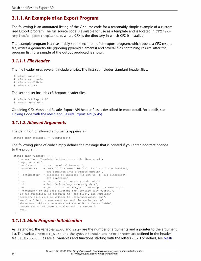
3.1.1. An Example of an Export Program
The following is an annotated listing of the C source code for a reasonably simple example of a custom-ized Export program. The full source code is available for use as a template and is located in CFX/ex-amples/ExportTemplate.c , where CFX is the directory in which CFX is installed.
The example program is a reasonably simple example of an export program, which opens a CFX resultsfile, writes a geometry file (ignoring pyramid elements) and several files containing results. After theprogram listing, a sample of the output produced is shown.
3.1.1.1. File Header
The file header uses several #include entries. The first set includes standard header files.
#include <stdio.h>#include <string.h>#include <stdlib.h>#include <io.h>
The second set includes cfx5export header files.
#include "cfxExport.h"#include "getargs.h"
Obtaining CFX-Mesh and Results Export API header files is described in more detail. For details, seeLinking Code with the Mesh and Results Export API (p. 45).
3.1.1.2. Allowed Arguments
The definition of allowed arguments appears as:
static char options[] = "u:d:t:cif";
The following piece of code simply defines the message that is printed if you enter incorrect optionsto the program.
static char *usgmsg[] = { "usage: ExportTemplate [options] res_file [basename]", " options are:", " -u<level> = user level of interest", " -d<domain> = domain of interest (default is 0 - all the domains", " are combined into a single domain)", " -t<timestep> = timestep of interest (if set to -1, all timesteps", " are exported)" " -c = use corrected boundary node data", " -i = include boundary node only data", " -f = get info on the res_file (No output is created)", " <basename> is the base filename for Template file output.", "If not specified, it defaults to ‘res_file’. The Template", "geometry file will be written to <basename>.geom, the", "results file to <basename>.res, and the variables to", "<basename>.s## or <basename>.v## where ## is the variable", "number and s indicates a scalar and v a vector.", NULL};
3.1.1.3. Main Program Initialization
As is standard, the variables argc and argv are the number of arguments and a pointer to the argumentlist. The variable cfxCNT_SIZE and the types cfxNode and cfxElement are defined in the headerfile cfxExport.h as are all variables and functions starting with the letters cfx . For details, see Mesh
Release 15.0 - © SAS IP, Inc. All rights reserved. - Contains proprietary and confidential informationof ANSYS, Inc. and its subsidiaries and affiliates.34
Mesh and Results Export API
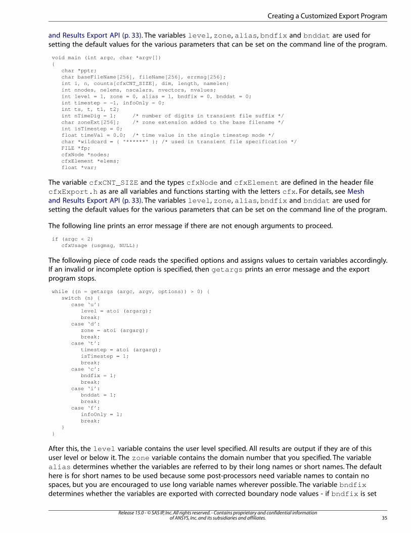
and Results Export API (p. 33). The variables level , zone , alias , bndfix and bnddat are used forsetting the default values for the various parameters that can be set on the command line of the program.
void main (int argc, char *argv[]){ char *pptr; char baseFileName[256], fileName[256], errmsg[256]; int i, n, counts[cfxCNT_SIZE], dim, length, namelen; int nnodes, nelems, nscalars, nvectors, nvalues; int level = 1, zone = 0, alias = 1, bndfix = 0, bnddat = 0; int timestep = -1, infoOnly = 0; int ts, t, t1, t2; int nTimeDig = 1; /* number of digits in transient file suffix */ char zoneExt[256]; /* zone extension added to the base filename */ int isTimestep = 0; float timeVal = 0.0; /* time value in the single timestep mode */ char *wildcard = { "******" }; /* used in transient file specification */ FILE *fp; cfxNode *nodes; cfxElement *elems; float *var;
The variable cfxCNT_SIZE and the types cfxNode and cfxElement are defined in the header filecfxExport.h as are all variables and functions starting with the letters cfx . For details, see Meshand Results Export API (p. 33). The variables level , zone , alias , bndfix and bnddat are used forsetting the default values for the various parameters that can be set on the command line of the program.
The following line prints an error message if there are not enough arguments to proceed.
if (argc < 2) cfxUsage (usgmsg, NULL);
The following piece of code reads the specified options and assigns values to certain variables accordingly.If an invalid or incomplete option is specified, then getargs prints an error message and the exportprogram stops.
while ((n = getargs (argc, argv, options)) > 0) { switch (n) { case ‘u’: level = atoi (argarg); break; case ‘d’: zone = atoi (argarg); break; case ‘t’: timestep = atoi (argarg); isTimestep = 1; break; case ‘c’: bndfix = 1; break; case ‘i’: bnddat = 1; break; case ‘f’: infoOnly = 1; break; }}
After this, the level variable contains the user level specified. All results are output if they are of thisuser level or below it. The zone variable contains the domain number that you specified. The variablealias determines whether the variables are referred to by their long names or short names. The defaulthere is for short names to be used because some post-processors need variable names to contain nospaces, but you are encouraged to use long variable names wherever possible. The variable bndfixdetermines whether the variables are exported with corrected boundary node values - if bndfix is set
35Release 15.0 - © SAS IP, Inc. All rights reserved. - Contains proprietary and confidential information
of ANSYS, Inc. and its subsidiaries and affiliates.
Creating a Customized Export Program

to 1, then corrected values are used. Finally, bnddat determines whether variables that containmeaningful values only on the boundary (such as Yplus) are exported or not; if bnddat is set to 1, thenthese variables are exported.
3.1.1.4. Checking File Names
The following code checks to make sure that a CFX results file has been specified, and that it can beread by the export program. If this is not the case, the export program exits.
/* CFX-5 results file */ if (argind >= argc) cfxUsage (usgmsg, "CFX-5 results file not specified"); if (access (argv[argind], 0)) { fprintf (stderr, "result file <%s> does not exist\n", argv[argind]); exit (1); }
The following code writes the basename specified to the character array baseFileName . If one wasnot specified, then it defaults to the name of the results file specified. A basename name may be specifiedin another directory (for example, “../template/output”). However, later in the code this basenamewithout the preceding directory information is required (in this example “output”); and so the pointerpptr is assigned to point to the first character of this name.
/* base file name */ if (argind + 1 < argc) strcpy (baseFileName, argv[argind+1]); else strcpy (baseFileName, argv[argind]);if (NULL != (pptr = strrchr (baseFileName, ‘/’))) pptr++; else if (NULL != (pptr = strrchr (baseFileName, ‘\\’))) pptr++; else pptr = baseFileName;
The following code checks that the results file that will be produced by the export program will notoverwrite an existing results file.
/* don’t overwrite results file */sprintf (fileName, "%s.res", baseFileName);if (0 == strcmp (argv[argind], fileName)) {fprintf (stderr, "Template res file would overwrite CFX results file\n");fprintf (stderr, "Need to select new Template output base file name\n");exit (1); }
3.1.1.5. Opening the CFX Results File
The following code prints a message to the screen telling you that the program is reading the resultsfile. It then calls cfxExportInit , which must always be called before any of the other export routines.The variable n is set to equal the number of zones in the results file. If the -f option has been selected,information about the results file will be displayed. The number of domains to be exported is also de-termined so that the format of the exported file includes the appropriate suffix. Finally, a check is madeto make sure that the zone (if any) that you specified in the program options is a valid zone for thisresults file.
/* open CFX-5 results file */printf ("\nreading CFX results from <%s>\n", argv[argind]); n = cfxExportInit (argv[argind], NULL); if (infoOnly) { int nt; printf("\n%d domains:\n", n); for(i = 1; i <= n; i++)
Release 15.0 - © SAS IP, Inc. All rights reserved. - Contains proprietary and confidential informationof ANSYS, Inc. and its subsidiaries and affiliates.36
Mesh and Results Export API
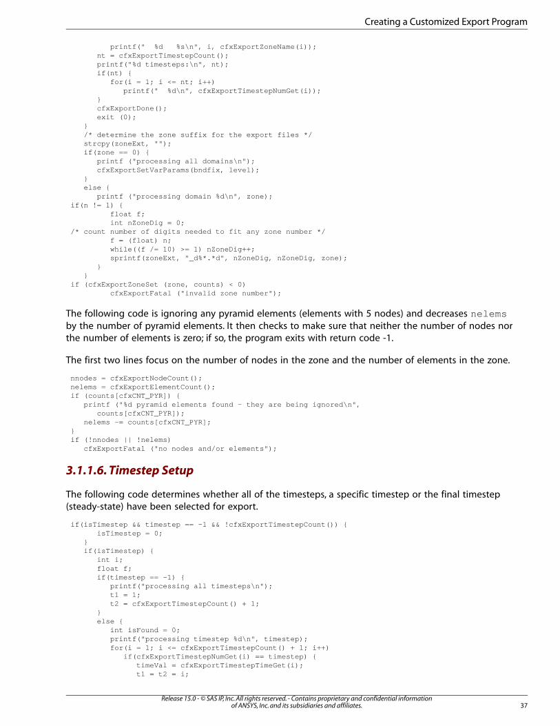
printf(" %d %s\n", i, cfxExportZoneName(i)); nt = cfxExportTimestepCount(); printf("%d timesteps:\n", nt); if(nt) { for(i = 1; i <= nt; i++) printf(" %d\n", cfxExportTimestepNumGet(i)); } cfxExportDone(); exit (0); } /* determine the zone suffix for the export files */ strcpy(zoneExt, ""); if(zone == 0) { printf ("processing all domains\n"); cfxExportSetVarParams(bndfix, level); } else { printf ("processing domain %d\n", zone);if(n != 1) { float f; int nZoneDig = 0;/* count number of digits needed to fit any zone number */ f = (float) n; while((f /= 10) >= 1) nZoneDig++; sprintf(zoneExt, "_d%*.*d", nZoneDig, nZoneDig, zone); } }if (cfxExportZoneSet (zone, counts) < 0) cfxExportFatal ("invalid zone number");
The following code is ignoring any pyramid elements (elements with 5 nodes) and decreases nelemsby the number of pyramid elements. It then checks to make sure that neither the number of nodes northe number of elements is zero; if so, the program exits with return code -1.
The first two lines focus on the number of nodes in the zone and the number of elements in the zone.
nnodes = cfxExportNodeCount();nelems = cfxExportElementCount();if (counts[cfxCNT_PYR]) { printf ("%d pyramid elements found - they are being ignored\n", counts[cfxCNT_PYR]); nelems -= counts[cfxCNT_PYR];}if (!nnodes || !nelems) cfxExportFatal ("no nodes and/or elements");
3.1.1.6. Timestep Setup
The following code determines whether all of the timesteps, a specific timestep or the final timestep(steady-state) have been selected for export.
if(isTimestep && timestep == -1 && !cfxExportTimestepCount()) { isTimestep = 0; } if(isTimestep) { int i; float f; if(timestep == -1) { printf("processing all timesteps\n"); t1 = 1; t2 = cfxExportTimestepCount() + 1; } else { int isFound = 0; printf("processing timestep %d\n", timestep); for(i = 1; i <= cfxExportTimestepCount() + 1; i++) if(cfxExportTimestepNumGet(i) == timestep) { timeVal = cfxExportTimestepTimeGet(i); t1 = t2 = i;
37Release 15.0 - © SAS IP, Inc. All rights reserved. - Contains proprietary and confidential information
of ANSYS, Inc. and its subsidiaries and affiliates.
Creating a Customized Export Program
isFound = 1; break; } if(!isFound) { sprintf(errmsg, "\nTimestep %d not found. " "Use -f to see the list of valid timesteps.\n", timestep); cfxExportFatal (errmsg); } } /* count number of digits needed to fit any timestep number */ f = (float) cfxExportTimestepCount(); while((f /= 10) >= 1) nTimeDig++; } else { timeVal = cfxExportTimestepTimeGet(cfxExportTimestepCount() + 1); timestep = cfxExportTimestepNumGet(cfxExportTimestepCount() + 1); t1 = t2 = cfxExportTimestepCount() + 1; }
3.1.1.7. Geometry File Output
The following code opens the geometry file basename.geom , printing an error if it cannot be openedfor any reason. A message is then displayed informing you that the application is writing the geometryfile.
/* Template geometry output */ sprintf (fileName, "%s.geom", baseFileName); if (NULL == (fp = fopen (fileName, "w+"))) { sprintf (errmsg, "can’t open <%s> for output", fileName); cfxExportFatal (errmsg); } printf ("writing Template Geometry file to <%s>\n", fileName);
The header of this file is shown after the program listing.
/* write header */ fprintf( fp, "Template Geometry file exported from CFX\n"); fprintf( fp, " \n"); fprintf( fp, "node id given\n"); fprintf( fp, "element id off\n");
The following code writes first the word "coordinates" and the number of nodes that will be written.The pointer nodes is initialized to point at the data for the first node and the node data is written intothe geometry file. For each node, a node number is written, followed by the three coordinates of thatnode. Note that n ranges between 0 and nnodes-1 . This program adds 1 to each node number sothat the nodes in the geometry file are numbered between 1 and nnodes . When it has finished, thecfxExportNodeFree routine frees the memory that was used to store the node data, and finally theword "done" is printed on the screen to alert you that it has finished writing the node data.
/* write nodes */ fprintf( fp, "coordinates\n"); fprintf( fp, "%8d\n", nnodes ); nodes = cfxExportNodeList(); printf (" writing %d nodes ...", nnodes); fflush (stdout); for (n = 0; n < nnodes; n++, nodes++) {fprintf( fp, "%8d %12.5e %12.5e %12.5e\n", n + 1, nodes->x, nodes->y, nodes->z );} cfxExportNodeFree();printf (" done\n");
Next, the data for each element must be written.
Firstly, some general information is written. Then the data for each element type is written in turn.
Release 15.0 - © SAS IP, Inc. All rights reserved. - Contains proprietary and confidential informationof ANSYS, Inc. and its subsidiaries and affiliates.38
Mesh and Results Export API
/* write elements */ fprintf( fp, "part 1\n" ); fprintf( fp, "volume elements\n"); printf (" writing %d elements...", nelems); fflush (stdout);
For tetrahedral elements, the word "tetra4" is written to the file, followed by the number of tetrahedralelements written.
/* tets */ fprintf( fp, "tetra4\n"); fprintf( fp, "%8d\n", counts[cfxCNT_TET] );
The following code is executed only if the number of tetrahedral elements is non-zero. Assuming this,elems is set to point to the list of elements stored in the results file. The index n loops over all theelements. For each element, the following step is carried out: “If the element is a tetrahedron, then loopover its four vertices and write their node numbers to the geometry file, then start a new line (readyfor the next set of data).” The output produced can be seen in the examples of the exported files inthe next section.
if (counts[cfxCNT_TET]) { elems = cfxExportElementList(); for (n = 0; n < nelems; n++, elems++) { if (cfxELEM_TET == elems->type) { for (i = 0; i < elems->type; i++) fprintf (fp, "%8d", elems->nodeid[i]); putc (‘\n’, fp); } }}
For wedges (triangular prisms) and hexahedral elements, the same procedure is followed. However,there is a slight difference in the way that the fprintf line is written for hexahedral elements. Thisis because the order that the element nodes are written to the geometry file is different to the orderin which they were read from the results file. This may need to be done if a post-processor has a differentconvention for node order than the one that the cfx5export node routines have. The order the nodesare written in will affect which node is connected to which. The node ordering for exported elementsis illustrated in cfxExportElementList (p. 52).
/* wedges */ fprintf( fp, "penta6\n"); fprintf( fp, "%8d\n", counts[cfxCNT_WDG] ); if (counts[cfxCNT_WDG]) { elems = cfxExportElementList(); for (n = 0; n < nelems; n++, elems++) { if (cfxELEM_WDG == elems->type) { for (i = 0; i < elems->type; i++) fprintf (fp, "%8d", elems->nodeid[i]); } putc (‘\n’, fp); } }/* hexes */ fprintf( fp, "hexa8\n"); fprintf( fp, "%8d\n", counts[cfxCNT_HEX] ); if (counts[cfxCNT_HEX]) { elems = cfxExportElementList(); for (n = 0; n < nelems; n++, elems++) { if (cfxELEM_HEX == elems->type) fprintf (fp, "%8d%8d%8d%8d%8d%8d%8d%8d\n", elems->nodeid[0], elems->nodeid[1], elems->nodeid[3], elems->nodeid[2], elems->nodeid[4], elems->nodeid[5], elems->nodeid[7], elems->nodeid[6]); } }
39Release 15.0 - © SAS IP, Inc. All rights reserved. - Contains proprietary and confidential information
of ANSYS, Inc. and its subsidiaries and affiliates.
Creating a Customized Export Program
Then the geometry file is closed and the memory occupied by the element data is freed.
printf (" done\n"); fclose (fp); cfxExportElementFree();
3.1.1.8. Template Results File
Despite its name, the Template results file does not contain any actual values of results. It simply containsinformation about how many variables there are and in which file each is stored.
The first job is to make sure that there are some results for export. First, the code checks that there isa nonzero number of variables that have the specified user level. Then it counts the number of scalarand vector variables that will be exported. To be exported, a variable must:
1. Have a dimension of 1 (scalar variable) or 3 (vector variable) and,
2. Either be a variable with useful values everywhere in the zone or be a variable that has values only onthe boundaries (in which case it will be exported only if you asked to "include boundary node onlydata" by specifying the option -i when starting the export program, which translated to setting bnddat= 1 when the arguments were processed).
Review the cfxExportVariableSize routine if this logic is unclear. For details, see cfxExportVari-ableSize (p. 58).
Once results are identified, the code calculates the variable namelen , which is the length of the longestvariable name to be exported (the alias variable was set when processing the arguments passed tothe export program, and depends upon whether you wanted to use long names or short names). Ifthere are no vector or scalar variables to be exported, the export program exits.
/* output results file */ nscalars = nvectors = namelen = 0; if ((nvalues = cfxExportVariableCount(level)) > 0) { for (n = 1; n <= nvalues; n++) { cfxExportVariableSize (n, &dim, &length, &i); if ((1 != dim && 3 != dim) || (length != nnodes && length != bnddat)) continue; if (1 == dim) nscalars++; else nvectors++; i = strlen (cfxExportVariableName (n, alias)); if (namelen < i) namelen = i; } } if (0 == (nscalars + nvectors)) { cfxExportDone (); exit (0); }
The following code checks that the results file can be opened for writing to, and exits if not. The numberof scalar and vector variables are written to the file, followed by some numbers (which EnSight, for ex-ample, requires) that are always the same for any export of this kind.
sprintf (fileName, "%s.res", baseFileName); if (NULL == (fp = fopen (fileName, "w+"))) { sprintf (errmsg, "can’t open <%s> for writing", fileName); cfxExportFatal (errmsg); } printf ("writing Template results file to <%s>\n", fileName); fflush (stdout);
Release 15.0 - © SAS IP, Inc. All rights reserved. - Contains proprietary and confidential informationof ANSYS, Inc. and its subsidiaries and affiliates.40
Mesh and Results Export API
fprintf( fp, "%d %d 0\n", nscalars, nvectors ); fprintf( fp, "%d\n", t2 - t1 + 1 ); for(i = t1; i <= t2; i++) { fprintf( fp, "%13.4e", cfxExportTimestepTimeGet(i)); if(!(i % 6)) fprintf( fp, "\n"); } fprintf( fp, "\n"); if(isTimestep && t1 != t2) fprintf( fp, "0 1\n");
Next, for each scalar variable, a line is written that contains the filename where the scalar will be written,and then the name of the variable. Note that the filename is not the basename, but the basename withall the directory structure (if any) stripped off the front. For details, see Checking File Names (p. 36).This is done because these file will be written in the same directory as this Template results file, so thereis no need for directory information.
if ( nscalars ) { for (n = 1; n <= nvalues; n++) { cfxExportVariableSize (n, &dim, &length, &i); if (1 == dim && (length == nnodes || length == bnddat)) if(!isTimestep) fprintf (fp, "%s%s.s%2.2d %s\n", pptr, zoneExt, n, cfxExportVariableName(n, alias)); else if(t1 == t2) fprintf (fp, "%s%s_t%d.s%2.2d %s\n", pptr, zoneExt, cfxExportTimestepNumGet(t1), n, cfxExportVariableName(n, alias)); else fprintf (fp, "%s%s_t%*.*s.s%2.2d %s\n", pptr, zoneExt, nTimeDig, nTimeDig, wildcard, n, cfxExportVariableName(n, alias)); } }
The same information is then written for each vector variable and the Template results file is closed.
if ( nvectors ) { for (n = 1; n <= nvalues; n++) { cfxExportVariableSize (n, &dim, &length, &i); if (3 == dim && (length == nnodes || length == bnddat)) if(!isTimestep) fprintf (fp, "%s%s.v%2.2d %s\n", pptr, zoneExt, n, cfxExportVariableName(n, alias)); else if(t1 == t2) fprintf (fp, "%s%s_t%d.v%2.2d %s\n", pptr, zoneExt, cfxExportTimestepNumGet(t1), n, cfxExportVariableName(n, alias)); else fprintf (fp, "%s%s_t%*.*s.v%2.2d %s\n", pptr, zoneExt, nTimeDig, nTimeDig, wildcard, n, cfxExportVariableName(n, alias)); } }fclose( fp );
3.1.1.9. Creating Files with Results for Each Variable
The results for each variable are written to separate files, called <basename>.s01 , <basename>.s02 ,<basename>.v03 , for example. Each file with an extension containing a letter “s” contains a scalarvariable, and each with a “v” contains a vector variable. Which variable is written to each file is tabulatedin the Template results file that has just been written.
The following code reads the information for each variable, after you decide that it should be exported- the logic is very similar to that used when counting the relevant variables when creating the Templateresults file. The marked if loop executes if the variable needs to be exported. It checks to make surethat the variable information can be read, and (assuming it can) then builds the filename and checks
41Release 15.0 - © SAS IP, Inc. All rights reserved. - Contains proprietary and confidential information
of ANSYS, Inc. and its subsidiaries and affiliates.
Creating a Customized Export Program
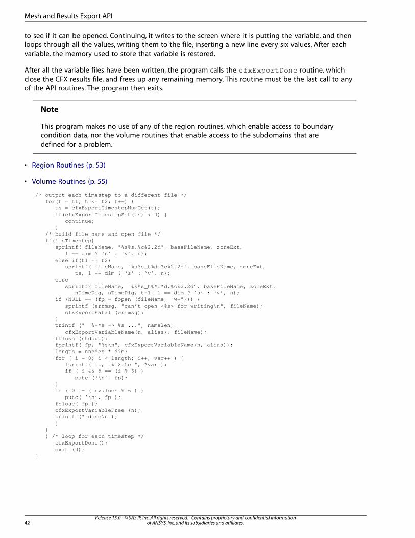
to see if it can be opened. Continuing, it writes to the screen where it is putting the variable, and thenloops through all the values, writing them to the file, inserting a new line every six values. After eachvariable, the memory used to store that variable is restored.
After all the variable files have been written, the program calls the cfxExportDone routine, whichclose the CFX results file, and frees up any remaining memory. This routine must be the last call to anyof the API routines. The program then exits.
Note
This program makes no use of any of the region routines, which enable access to boundarycondition data, nor the volume routines that enable access to the subdomains that aredefined for a problem.
• Region Routines (p. 53)
• Volume Routines (p. 55)
/* output each timestep to a different file */ for(t = t1; t <= t2; t++) { ts = cfxExportTimestepNumGet(t); if(cfxExportTimestepSet(ts) < 0) { continue; } /* build file name and open file */ if(!isTimestep) sprintf( fileName, "%s%s.%c%2.2d", baseFileName, zoneExt, 1 == dim ? ‘s’ : ‘v’, n); else if(t1 == t2) sprintf( fileName, "%s%s_t%d.%c%2.2d", baseFileName, zoneExt, ts, 1 == dim ? ‘s’ : ‘v’, n); else sprintf( fileName, "%s%s_t%*.*d.%c%2.2d", baseFileName, zoneExt, nTimeDig, nTimeDig, t-1, 1 == dim ? ‘s’ : ‘v’, n); if (NULL == (fp = fopen (fileName, "w+"))) { sprintf (errmsg, "can’t open <%s> for writing\n", fileName); cfxExportFatal (errmsg); } printf (" %-*s -> %s ...", namelen, cfxExportVariableName(n, alias), fileName); fflush (stdout); fprintf( fp, "%s\n", cfxExportVariableName(n, alias)); length = nnodes * dim; for ( i = 0; i < length; i++, var++ ) { fprintf( fp, "%12.5e ", *var ); if ( i && 5 == (i % 6) ) putc (‘\n’, fp); } if ( 0 != ( nvalues % 6 ) ) putc( ‘\n’, fp ); fclose( fp ); cfxExportVariableFree (n); printf (" done\n"); } } } /* loop for each timestep */ cfxExportDone(); exit (0);}
Release 15.0 - © SAS IP, Inc. All rights reserved. - Contains proprietary and confidential informationof ANSYS, Inc. and its subsidiaries and affiliates.42
Mesh and Results Export API
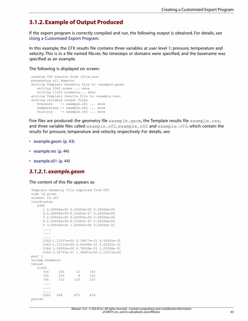
3.1.2. Example of Output Produced
If the export program is correctly compiled and run, the following output is obtained. For details, seeUsing a Customized Export Program.
In this example, the CFX results file contains three variables at user level 1: pressure, temperature andvelocity. This is in a file named file.res. No timesteps or domains were specified, and the basename wasspecified as an example.
The following is displayed on screen:
reading CFX results from <file.res>processing all domainswriting Template Geometry file to <example.geom> writing 2365 nodes ... done writing 11435 elements... donewriting Template results file to <example.res>writing variable output files Pressure -> example.s01 ... done Temperature -> example.s02 ... done Velocity -> example.v03 ... done
Five files are produced: the geometry file example.geom , the Template results file example.res ,and three variable files called example.s01 , example.s02 and example.v03 , which contain theresults for pressure, temperature and velocity, respectively. For details, see:
• example.geom (p. 43)
• example.res (p. 44)
• example.s01 (p. 44)
3.1.2.1. example.geom
The content of this file appears as:
Template Geometry file exported from CFXnode id givenelement id offcoordinates 2365 1 2.00000e+00 0.00000e+00 0.00000e+00 2-2.00000e+00-6.51683e-07 0.00000e+00 3 2.00000e+00 0.00000e+00 2.00000e+00 4-2.00000e+00-6.51683e-07 2.00000e+00 5 3.00000e+00 1.00000e+00 5.00000e-01 .... .... .... 2362-1.13337e+00 2.18877e-01 4.02491e-01 2363-1.12115e+00-3.66598e-01 2.22610e-01 2364 1.36924e+00 4.78359e-01 1.22588e-01 2365-3.30703e-01 1.38487e+00 2.23515e+00part 1volume elementstetra4 11435 754 230 12 145 755 216 8 122 756 212 125 215 .... .... .... 2365 496 475 474penta6
43Release 15.0 - © SAS IP, Inc. All rights reserved. - Contains proprietary and confidential information
of ANSYS, Inc. and its subsidiaries and affiliates.
Creating a Customized Export Program
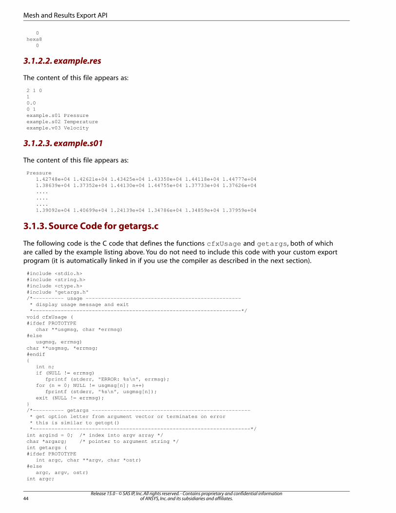
0hexa8 0
3.1.2.2. example.res
The content of this file appears as:
2 1 010.00 1example.s01 Pressureexample.s02 Temperatureexample.v03 Velocity
3.1.2.3. example.s01
The content of this file appears as:
Pressure 1.42748e+04 1.42621e+04 1.43425e+04 1.43350e+04 1.44118e+04 1.44777e+04 1.38639e+04 1.37352e+04 1.44130e+04 1.44755e+04 1.37733e+04 1.37626e+04 .... .... .... 1.39092e+04 1.40699e+04 1.24139e+04 1.34786e+04 1.34859e+04 1.37959e+04
3.1.3. Source Code for getargs.c
The following code is the C code that defines the functions cfxUsage and getargs , both of whichare called by the example listing above. You do not need to include this code with your custom exportprogram (it is automatically linked in if you use the compiler as described in the next section).
#include <stdio.h>#include <string.h>#include <ctype.h>#include "getargs.h"/*---------- usage -------------------------------------------------- * display usage message and exit *-------------------------------------------------------------------*/void cfxUsage (#ifdef PROTOTYPE char **usgmsg, char *errmsg)#else usgmsg, errmsg)char **usgmsg, *errmsg;#endif{ int n; if (NULL != errmsg) fprintf (stderr, "ERROR: %s\n", errmsg); for (n = 0; NULL != usgmsg[n]; n++) fprintf (stderr, "%s\n", usgmsg[n]); exit (NULL != errmsg);}/*---------- getargs --------------------------------------------------- * get option letter from argument vector or terminates on error * this is similar to getopt() *----------------------------------------------------------------------*/int argind = 0; /* index into argv array */char *argarg; /* pointer to argument string */int getargs (#ifdef PROTOTYPE int argc, char **argv, char *ostr)#else argc, argv, ostr)int argc;
Release 15.0 - © SAS IP, Inc. All rights reserved. - Contains proprietary and confidential informationof ANSYS, Inc. and its subsidiaries and affiliates.44
Mesh and Results Export API
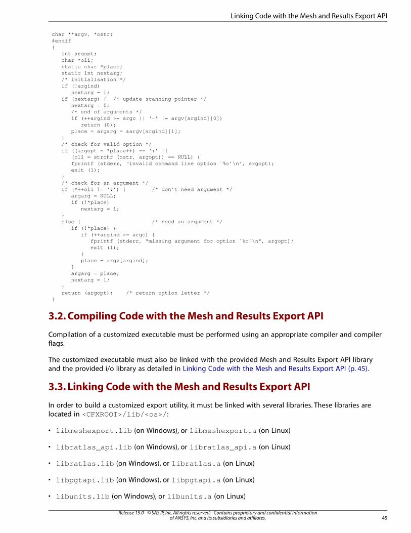
char **argv, *ostr;#endif{ int argopt; char *oli; static char *place; static int nextarg; /* initialisation */ if (!argind) nextarg = 1; if (nextarg) { /* update scanning pointer */ nextarg = 0; /* end of arguments */ if (++argind >= argc || ‘-’ != argv[argind][0]) return (0); place = argarg = &argv[argind][1]; } /* check for valid option */ if ((argopt = *place++) == ‘:’ || (oli = strchr (ostr, argopt)) == NULL) { fprintf (stderr, "invalid command line option `%c’\n", argopt); exit (1); } /* check for an argument */ if (*++oli != ‘:’) { /* don’t need argument */ argarg = NULL; if (!*place) nextarg = 1; } else { /* need an argument */ if (!*place) { if (++argind >= argc) { fprintf (stderr, "missing argument for option `%c’\n", argopt); exit (1); } place = argv[argind]; } argarg = place; nextarg = 1; } return (argopt); /* return option letter */}
3.2. Compiling Code with the Mesh and Results Export API
Compilation of a customized executable must be performed using an appropriate compiler and compilerflags.
The customized executable must also be linked with the provided Mesh and Results Export API libraryand the provided i/o library as detailed in Linking Code with the Mesh and Results Export API (p. 45).
3.3. Linking Code with the Mesh and Results Export API
In order to build a customized export utility, it must be linked with several libraries. These libraries arelocated in <CFXROOT>/lib/< os>/ :
• libmeshexport.lib (on Windows), or libmeshexport.a (on Linux)
• libratlas_api.lib (on Windows), or libratlas_api.a (on Linux)
• libratlas.lib (on Windows), or libratlas.a (on Linux)
• libpgtapi.lib (on Windows), or libpgtapi.a (on Linux)
• libunits.lib (on Windows), or libunits.a (on Linux)
45Release 15.0 - © SAS IP, Inc. All rights reserved. - Contains proprietary and confidential information
of ANSYS, Inc. and its subsidiaries and affiliates.
Linking Code with the Mesh and Results Export API
• libcclapilt.lib (on Windows), or libcclapilt.a (on Linux)
• libio.lib (on Windows), or libio.a (on Linux)
3.3.1. UNIX
On most UNIX systems, build the executable with the command:
cc export.c -o export.exe -I<CFXROOT>/include/ -L<CFXROOT>/lib/< OSDIR> -lmeshexport -lratlas_api -lratlas -lpgtapi -lcclapilt -lunits -lio -lm -lc
where <CFXROOT> is the directory in which CFX is installed and <OSDIR> is a directory name corres-ponding to the architecture of the machine. In this example, your own export program is named ex-port.c and the executable file will be called export.exe .
The compiler flags and required libraries may vary, depending on the compiler and the custom program.
You can use the GCC compiler v4.6.1 with ANSYS CFX 15.0.
3.3.2. Windows (32-bit)
You can build the executables on 32-bit Windows systems that have the C++ compiler of MicrosoftVisual Studio 2010. An example command line follows:
cl /MD /I "C:\Program Files\Ansys Inc\v150\CFX\include" ExportTemplate.c/link /libpath:"C:\Program Files\Ansys Inc\v150\CFX\lib\winnt" lib-cclapilt.lib libio.lib libmeshexport.lib libunits.lib libpgtapi.lib lib-ratlas_api.lib libratlas.lib
3.3.3. Windows (64-bit)
You can build the executables on 64-bit Windows systems that have the C++ compiler of MicrosoftVisual Studio 2010. An example command line follows:
cl /MD /I "C:\Program Files\Ansys Inc\v150\CFX\include" ExportTemplate.c/link /libpath:"C:\Program Files\Ansys Inc\v150\CFX\lib\winnt-amd64"libcclapilt.lib libio.lib libmeshexport.lib libunits.lib libpgtapi.liblibratlas_api.lib libratlas.lib
3.4. Details of the Mesh Export API
The full list of constants, data structures, types and functions available to the programmer are given inthe following sections:
3.4.1. Defined Constants and Structures3.4.2. Initialization and Error Routines3.4.3. Zone Routines3.4.4. Node Routines3.4.5. Element Routines3.4.6. Region Routines3.4.7. Face Routines3.4.8.Volume Routines3.4.9. Boundary Condition Routines3.4.10.Variable Routines
Release 15.0 - © SAS IP, Inc. All rights reserved. - Contains proprietary and confidential informationof ANSYS, Inc. and its subsidiaries and affiliates.46
Mesh and Results Export API

3.4.1. Defined Constants and Structures
The following constants and data structures are defined in the header file cfxExport.h , which shouldbe included in the export program.
3.4.1.1. Element Types
CFX can use 4 types of element, which are identified by the number of nodes: tetrahedrons (4 nodes),pyramids (5 nodes), prisms/wedges (6 nodes), and hexahedrons (8 nodes). The element types areidentified in the Export API by the following constants:
#define cfxELEM_TET 4 #define cfxELEM_PYR 5 #define cfxELEM_WDG 6 #define cfxELEM_HEX 8
3.4.1.2. Volume List Types
The Export API contains functions that enable you to query how volumes are defined in the results file.It is possible to request how a volume is defined in terms of nodes or elements. (For details, see VolumeRoutines (p. 55).)
The following constants are defined in the header file and should be used as arguments to the Volumeroutines:
#define cfxVOL_NODES 0#define cfxVOL_ELEMS 1
3.4.1.3. Region List Types
The Export API contains functions that enable you to query how regions are defined in the results file.It is possible to request how a region is defined in terms of nodes or faces. (For details, see RegionRoutines (p. 53).)
The following constants are defined in the header file and should be used as arguments to the Regionroutines:
#define cfxREG_NODES 0#define cfxREG_FACES 1
In the case of nodes, the global node number is returned, while in the case of faces, the returned valueis a combination of the global element number and local face number of the element. The followingmacros are available to enable you to extract the element and face number from the combined value:
#define cfxFACENUM(face) ((face) & 7)#define cfxELEMNUM(face) ((face) >> 3)
3.4.1.4. Count Entries
Two routines exist for initializing the Export API (see cfxExportInit (p. 48)) and requesting the totals ofcertain quantities in a zone (see cfxExportZoneSet (p. 49)). The array returned from both of theseroutines requires the following constants to be used by the calling program to reference the correctquantities.
enum cfxCounts { cfxCNT_NODE = 0, /* number of nodes */ cfxCNT_ELEMENT, /* number of elements */ cfxCNT_VOLUME, /* number of volumes */cfxCNT_REGION, /* number of regions */
47Release 15.0 - © SAS IP, Inc. All rights reserved. - Contains proprietary and confidential information
of ANSYS, Inc. and its subsidiaries and affiliates.
Details of the Mesh Export API
cfxCNT_VARIABLE, /* number of variables */cfxCNT_TET, /* number of tetrahedral elements */ cfxCNT_PYR, /* number of pyramid elements */ cfxCNT_WDG, /* number of wedge elements */ cfxCNT_HEX, /* number of hexahedral elements */cfxCNT_SIZE /* size of count array */};
3.4.1.5. Node Data Structure
Nodes are represented in the Export API using the following structure (note the change in data typeof x, y and z):
typedef struct cfxNode { float x, y, z; } cfxNode;
where x , y , and z are the coordinates of the node. A pointer to an array of these structures is returnedby cfxExportNodeList . For details, see cfxExportNodeList (p. 51).
3.4.1.6. Element Data Structure
Elements are represented by the Export API using the following structure:
typedef struct cfxElement {int type; int *nodeid; } cfxElement;
where type is the element type and nodeid is an array of node numbers that define the topology ofthe element. A pointer to an array of these structures is returned by cfxExportElementList . Fordetails, see Element Types (p. 47) and cfxExportElementList (p. 52).
3.4.2. Initialization and Error Routines
The following routines open and close the CFX results file, initialize the Export API, and handle fatalerror processing. The first call to any of the API routines must be cfxExportInit and the last callshould be cfxExportDone . For details, see:
• cfxExportInit (p. 48)
• cfxExportDone (p. 48).
3.4.2.1. cfxExportInit
int cfxExportInit (char *resfile, int counts[cfxCNT_SIZE])
Opens the CFX results file named resfile and initializes the Export API. This should be the first callmade to the API.
The routine returns the total number of zones. If the array counts is supplied to the routine (that is,it is not NULL), the array is filled with values representing the total number of nodes, elements, volumes,regions and variables for all the zones are returned in this array.
3.4.2.2. cfxExportDone
void cfxExportDone ()
Release 15.0 - © SAS IP, Inc. All rights reserved. - Contains proprietary and confidential informationof ANSYS, Inc. and its subsidiaries and affiliates.48
Mesh and Results Export API
Closes the CFX results file and destroys any internal storage used by the API. This should be the finalcall made to the Export API.
3.4.2.3. cfxExportError
void cfxExportError (void (*callback) (char *errmsg))
Specify a callback function that will be executed when a fatal error is generated by a call to cfxImportFatal (see cfxImportFatal (p. 16)). The argument, callback, is the function that will be called, itshould take an argument that is the error message passed to cfxImportFatal. It is the responsibility ofthe function to terminate the application if required.
3.4.2.4. cfxExportFatal
void cfxExportFatal (char *errmsg)
Generate a fatal error message (errmsg ) and close the ANSYS CFX results file. This routine also calls acallback function, if one has been specified by cfxExportError (see cfxExportError (p. 49)). If nocallback function has been specified the function also terminates the application. There is no returnfrom this call.
3.4.3. Zone Routines
A zone is defined as groups of nodes or faces that are located on the external boundaries of the domain.The following routines provide functionality for returning the number of zones in the open CFX resultsfile specifying and requesting the current zone, and destroying any internal storage associated with azone. All other routines in the Export API refer to quantities in the current zone being accessed by theAPI. By default the current zone is the global zone (a combination of all zones in the ANSYS CFX resultsfile), but this can be the current zone can be altered by making a call to cfxExportZoneSet (seecfxExportZoneSet (p. 49)). Once this call has been made, any other function returns information aboutthis zone until a subsequent call is made.
3.4.3.1. cfxExportZoneCount
int cfxExportZoneCount ()
Return the number of zones in the CFX results file.
3.4.3.2. cfxExportZoneSet
int cfxExportZoneSet (int zone, int counts[cfxCNT_SIZE])
Set the current zone being accessed by the Export API.
The value of zone should be between 1 and the value returned by cfxExportZoneCount (see cfxEx-portZoneCount (p. 49)) or 0 if the global zone is to be accessed.
The function returns 0 if the value of zone is invalid or the value zone if setting of the zone was successful.
The argument counts can be passed as a NULL pointer. In this case no information is returned to thecalling function other than the return value mentioned above. If counts is specified it must be at leastcfxCNT_SIZE in size, not specifying an array large enough can result in errors. In the case when countsis supplied correctly the total number of nodes, elements, volumes, regions and variables will be returned.
49Release 15.0 - © SAS IP, Inc. All rights reserved. - Contains proprietary and confidential information
of ANSYS, Inc. and its subsidiaries and affiliates.
Details of the Mesh Export API
3.4.3.3. cfxExportZoneGet
int cfxExportZoneGet ()
Returns the current zone number.
3.4.3.4. cfxExportZoneFree
void cfxExportZoneFree ()
While a zone is being accessed, internal storage is allocated, this storage should be deallocated whenno longer required. This can be done by calling cfxExportZoneFree or by calling cfxExportNodeFree , cfxExportElementFree , cfxExportVolumeFree , cfxExportRegionFree and cfxExportVariableFree . Details on each of these routines is available; see:
• cfxExportNodeFree (p. 51)
• cfxExportElementFree (p. 53)
• cfxExportVolumeFree (p. 56)
• cfxExportRegionFree (p. 54)
• cfxExportVariableFree (p. 60).
3.4.3.5. cfxExportZoneIsRotating
int cfxExportZoneIsRotating(double rotationAxis[2][3], double *angularVelocity)
Query whether the current zone is rotating and describe axis and angular velocity of the rotation ifapplicable. Returns 1 if the current zone is rotating and 0 if it is not; for the combined zone the returnvalue is always -1. If successful the rotation axis is returned in rotationAxis and the velocity in angularVelocity in radians/second.
3.4.3.6. cfxExportZoneMotionAction
int cfxExportZoneMotionAction(const int zone, const int flag)
Specify whether grid coordinates and variables should have the appropriate rotation applied to themif the zone is rotating so that grid coordinates appear in their correct locations and velocities (for ex-amples) take this rotation into consideration. If cfxExportZoneList and cfxExportVariableListshould return rotated values, flag should be set to cfxMOTION_USE. The default behavior for a partic-ular zone will be used if cfxMOTION_IGNORE is specified or this function is not called. If zone is notvalid or flag is not cfxMOTION_USE, cfxMOTION_IGNORE the return value will be -1 otherwise 0 isreturned.
3.4.4. Node Routines
Accessing nodes within the current zone (see cfxExportZoneSet (p. 49)) is performed by making callsto the following functions.
It should be noted that the nodes for a zone are not loaded into the Export API until either cfxExportNodeList (see cfxExportNodeList (p. 51)) or cfxExportNodeGet (see cfxExportNodeGet (p. 51))are called. This reduces memory overheads in the API by not allocating space until required.
Release 15.0 - © SAS IP, Inc. All rights reserved. - Contains proprietary and confidential informationof ANSYS, Inc. and its subsidiaries and affiliates.50
Mesh and Results Export API
When access to nodes in the current zone is no longer required, a call to cfxExportNodeFree (seecfxExportNodeFree (p. 51)) should be made to deallocate any internal storage.
3.4.4.1. cfxExportNodeCount
int cfxExportNodeCount ()
Query the number of nodes defined in the current zone.
3.4.4.2. cfxExportNodeList
cfxNode *cfxExportNodeList ()
Return a pointer to an array of cfxNode elements (see cfxnode (p. 23)) containing the coordinate valuesof each node in the current zone. The first node in the zone is the first element of the array, the secondis the second and so on.
The memory allocated to represent this information should be deallocated using cfxExportNodeFree(see cfxExportNodeFree (p. 51)) when no longer required.
3.4.4.3. cfxExportNodeGet
int cfxExportNodeGet (int nodeid, double *x, double *y, double *z)
Query the coordinates of a specific node in the current zone.
The index (nodeid) is specified between 1 and the number of nodes returned by cfxExportNodeCount(see cfxExportNodeCount (p. 51)). If the value of nodeid is out of range the return value is 0 otherwiseit is nodeid.
3.4.4.4. cfxExportNodeFree
void cfxExportNodeFree ()
Deallocate any internal storage allocated by the Export API after calls to cfxExportNodeList (seecfxExportNodeList (p. 51)) and cfxExportNodeGet (see cfxExportNodeGet (p. 51)) have been madein the current zone.
3.4.5. Element Routines
Accessing elements within the current zone (see cfxExportZoneSet (p. 49)) is performed by making callsto the following functions. It should be noted that the elements for a zone are not loaded into the ExportAPI until either cfxExportElementList (see cfxExportElementList (p. 52)) or cfxExportElementGet (see cfxExportElementGet (p. 52)) are called. This reduces memory overheads in the API by notallocating space until required.
When access to elements in the current zone is no longer required a call to cfxExportElementFree(see cfxExportElementFree (p. 53)) should be made to deallocate any internal storage.
3.4.5.1. cfxExportElementCount
int cfxExportElementCount ()
Query the number of elements defined in the current zone.
51Release 15.0 - © SAS IP, Inc. All rights reserved. - Contains proprietary and confidential information
of ANSYS, Inc. and its subsidiaries and affiliates.
Details of the Mesh Export API
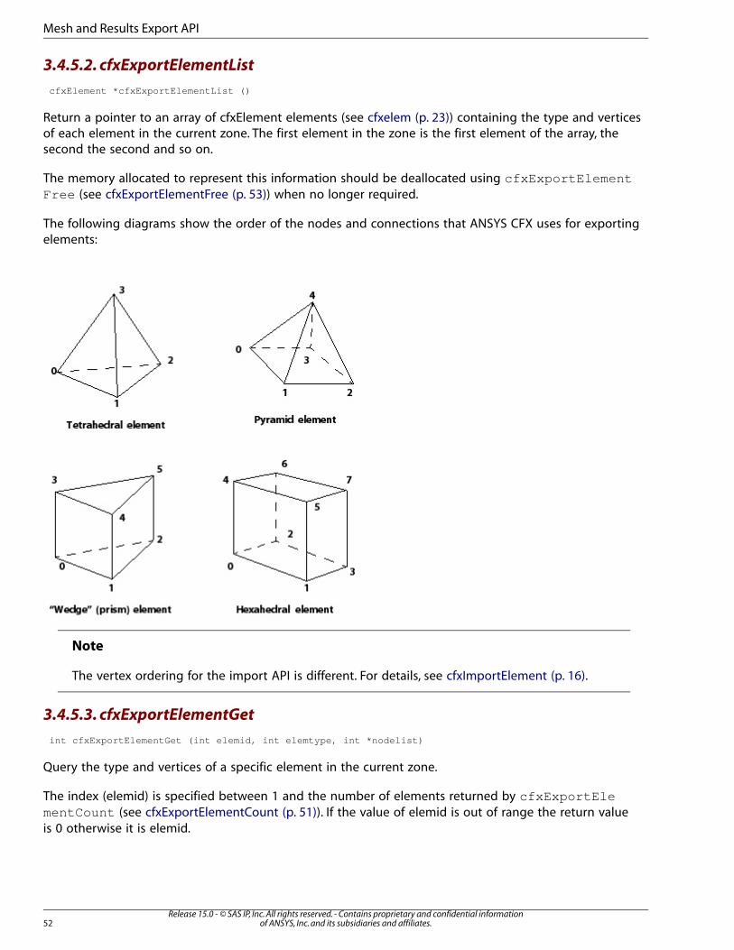
3.4.5.2. cfxExportElementList
cfxElement *cfxExportElementList ()
Return a pointer to an array of cfxElement elements (see cfxelem (p. 23)) containing the type and verticesof each element in the current zone. The first element in the zone is the first element of the array, thesecond the second and so on.
The memory allocated to represent this information should be deallocated using cfxExportElementFree (see cfxExportElementFree (p. 53)) when no longer required.
The following diagrams show the order of the nodes and connections that ANSYS CFX uses for exportingelements:
Note
The vertex ordering for the import API is different. For details, see cfxImportElement (p. 16).
3.4.5.3. cfxExportElementGet
int cfxExportElementGet (int elemid, int elemtype, int *nodelist)
Query the type and vertices of a specific element in the current zone.
The index (elemid) is specified between 1 and the number of elements returned by cfxExportElementCount (see cfxExportElementCount (p. 51)). If the value of elemid is out of range the return valueis 0 otherwise it is elemid.
Release 15.0 - © SAS IP, Inc. All rights reserved. - Contains proprietary and confidential informationof ANSYS, Inc. and its subsidiaries and affiliates.52
Mesh and Results Export API
The type of the element is returned in elemtype and the vertices defining the element in nodelist. Notethat nodelist must be large enough to hold the element number of vertices in the element (normallyan array of 8 integers is used as this allows space enough for all element types to be handled).
3.4.5.4. cfxExportElementFree
void cfxExportElementFree ()
Deallocates any internal storage allocated by making calls to cfxExportElementList (see cfxExpor-tElementList (p. 52)) or cfxExportElementGet (see cfxExportElementGet (p. 52)).
3.4.6. Region Routines
Regions are groups of faces in an ANSYS CFX results file. Accessing regions within the current zone (seecfxExportZoneSet (p. 49)) is performed by making calls to the following functions. It should be notedthat the region information is not loaded into the Export API until either cfxExportRegionList(see cfxExportRegionList (p. 53)) or cfxExportRegionGet (see cfxExportRegionGet (p. 54)) are called.This reduces memory overheads in the API by not allocating space until required.
When access to region in the current zone is no longer required a call to cfxExportRegionFree(see cfxExportRegionFree (p. 54)) should be made to deallocate any internal storage.
3.4.6.1. cfxExportRegionCount
int cfxExportRegionCount ()
Query the number of regions defined in the current zone.
3.4.6.2. cfxExportRegionSize
int cfxExportRegionSize (int regnum, int type)
Query the number of faces (if type is cfxREG_FACES) or nodes (if type is cfxREG_NODES) definedin the region identified by regnum in the current zone.
The function returns the number of faces or nodes in the current zone or 0 if either regnum is out ofrange or type is invalid.
3.4.6.3. cfxExportRegionName
char *cfxExportRegionName (int regnum)
Query the name of the region in the current zone identifies by regnum.
The function returns the name of the region or NULL if the region number supplied is out of range.The pointer returned points to static storage, which will be overwritten by the next call to cfxExportRegionName .
3.4.6.4. cfxExportRegionList
int *cfxExportRegionList (int regnum, int type)
Query the nodes (type is cfxREG_NODES) or faces (cfxREG_FACES) that define a region. This functionreturns a pointer to an array of node ids or face ids that define the region identified by regnum or NULLif the region number is out of range or the type is not recognized. If type is specified as cfxREG_FACES,the returned ids will represent faces. The element number and local element face number may be ex-
53Release 15.0 - © SAS IP, Inc. All rights reserved. - Contains proprietary and confidential information
of ANSYS, Inc. and its subsidiaries and affiliates.
Details of the Mesh Export API
tracted from each face id returned by using the macros cfxELEMNUM and cfxFACENUM. The nodenumbers for the face may be obtained by calling cfxExportFaceNodes . For details, see cfxExport-FaceNodes (p. 54).
3.4.6.5. cfxExportRegionGet
int cfxExportRegionGet (int regnum, int type, int index, int *id)
Query the index’th element (type is cfxREG_ELEM) or index’th node (type is cfxREG_NODE) thatdefines a the region regnum in the current zone.
If regnum is out of range or type is not recognized or index is out of range, 0 is returned.
Otherwise id will contain the id of the appropriate node or face defining the region and the functionwill return index.
If type is specified as cfxREG_FACES, the returned id will represent the identity of a face. The elementnumber and local element face number may be extracted from the id by using the macros cfxELEMNUMand cfxFACENUM.
3.4.6.6. cfxExportRegionFree
void cfxExportRegionFree (int regnum)
Deallocate any internal data storage associated with the region defined by regnum .
3.4.7. Face Routines
Faces are 2 dimensional (2D) units of mesh. Each global face ID is returned from cfxExportBoundaryList (see cfxExportBoundaryList (p. 57)) or cfxExportRegionList (see cfxExportRegionList (p. 53)).
Within CFX faces are either represented as Triangles (three vertices) or Quadrilaterals (two vertices).Each face in a CFX .res file will be parented by a single 3D element. The parent element of a face canbe returned by the cfxELEMNUM macro with the global face ID, and the local face of that element canbe determined by calling cfxFACENUM with the same global face ID
3.4.7.1. cfxExportFaceNodes
int cfxExportFaceNodes (int faceid, int *nodes)
Requests the vertices for the face identified by faceid . The argument faceid should be constructedfrom the element number and local face number using the following formula:
(element_number << 3) & local_face_number
Values returned from cfxExportRegionGet and cfxExportRegionList can be supplied directlyto this function.
The number of vertices defining the face are returned if faceid is valid, otherwise 0 is returned. Thenode numbers are returned in the array nodes , which should be dimensioned to a minimum size of 4in the calling routine.
The face numbers and associated node indices are tabulated here:
Release 15.0 - © SAS IP, Inc. All rights reserved. - Contains proprietary and confidential informationof ANSYS, Inc. and its subsidiaries and affiliates.54
Mesh and Results Export API
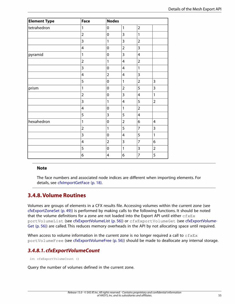
NodesFaceElement Type
2101tetrahedron
1302
2313
3204
4301pyramid
2412
1403
3424
32105
35201prism
14302
25413
2104
4535
46201hexahedron
37512
15403
67324
23105
57646
Note
The face numbers and associated node indices are different when importing elements. Fordetails, see cfxImportGetFace (p. 18).
3.4.8. Volume Routines
Volumes are groups of elements in a CFX results file. Accessing volumes within the current zone (seecfxExportZoneSet (p. 49)) is performed by making calls to the following functions. It should be notedthat the volume definitions for a zone are not loaded into the Export API until either cfxExportVolumeList (see cfxExportVolumeList (p. 56)) or cfxExportVolumeGet (see cfxExportVolume-Get (p. 56)) are called. This reduces memory overheads in the API by not allocating space until required.
When access to volume information in the current zone is no longer required a call to cfxExportVolumeFree (see cfxExportVolumeFree (p. 56)) should be made to deallocate any internal storage.
3.4.8.1. cfxExportVolumeCount
int cfxExportVolumeCount ()
Query the number of volumes defined in the current zone.
55Release 15.0 - © SAS IP, Inc. All rights reserved. - Contains proprietary and confidential information
of ANSYS, Inc. and its subsidiaries and affiliates.
Details of the Mesh Export API
3.4.8.2. cfxExportVolumeSize
int cfxExportVolumeSize (int volnum, int type)
Query the number of nodes (if type is cfxVOL_NODES) or number of elements (if type is cfxVOL_ELEMS) defining the volume indexed by volnum in the current zone. The return value will be 0if volnum is out of range or type is invalid.
3.4.8.3. cfxExportVolumeName
char *cfxExportVolumeName (int volnum)
Query the name of the volume in the current zone indexed by volnum . Returns NULL if the volnumis out of range.
Note
The returned pointer points to internal storage, which will be overwritten by the next callto cfxExportVolumeName .
3.4.8.4. cfxExportVolumeList
int *cfxExportVolumeList (int volnum, int type)
Query the nodes (type is cfxVOL_NODES) or elements (cfxVOL_ELEMS) that define a volume.
This function returns a pointer to an array of node ids or element ids that define the volume identifiedby volnum or NULL if the volume number is out of range or the type is not recognized.
3.4.8.5. cfxExportVolumeGet
int cfxExportVolumeGet (int volnum, int type, int index, int *id)
Query the [index]th element (type is cfxVOL_ELEM) or [index]th node (type is cfxVOL_NODE) thatdefines a the volume volnum in the current zone.
If volnum is out of range or type is not recognized or index is out of range, 0 is returned.
Otherwise id will contain the id of the appropriate node or element in defining the volume and thefunction will return index .
3.4.8.6. cfxExportVolumeFree
void cfxExportVolumeFree (int volnum)
Deallocate any internal data storage associated with the volume defined by volnum .
3.4.9. Boundary Condition Routines
Boundary condition are located on groups of faces in a CFX results file. Accessing boundary conditionlocations within the current zone (see cfxExportZoneSet (p. 49)) is performed by making calls to thefollowing functions. It should be noted that the boundary condition location information is not loadedinto the Export API until either cfxExportBoundaryList (see cfxExportBoundaryList (p. 57)) orcfxExportBoundaryGet (see cfxExportBoundaryGet (p. 58)) are called. This reduces memory over-heads in the API by not allocating space until required. When access to regions in the current zone are
Release 15.0 - © SAS IP, Inc. All rights reserved. - Contains proprietary and confidential informationof ANSYS, Inc. and its subsidiaries and affiliates.56
Mesh and Results Export API
no longer required a call to cfxExportBoundaryFree (see cfxExportBoundaryFree (p. 58)) shouldbe made to deallocate any internal storage.
3.4.9.1. cfxExportBoundaryCount
int cfxExportBoundaryCount ()
Query the number of boundary conditions defined in the current zone.
The function returns the number of boundary conditions in the current zone.
3.4.9.2. cfxExportBoundaryName
const char *cfxExportBoundaryName (const int bcidx)
Query the name of the boundary condition in the current zone identified by bcidx .
The function returns the name of the boundary condition or NULL if the bcidx supplied is out ofrange.
The pointer returned points to static storage, which will be overwritten by the next call to cfxExportBoundaryName .
Note
The following routines use bcidx which must lie between 1 and cfxExportBoundaryCount() and use index which must lie between 1 and cfxExportBoundarySize (bcidx,type).
3.4.9.3. cfxExportBoundaryType
const char *cfxExportBoundaryType (const int bcidx)
Query the type (for example, Inlet, Outlet etc.) of the boundary condition in the current zone identifiedby bcidx .
The function returns the type of the boundary condition or NULL if the bcidx supplied is out of range.
The pointer returned points to static storage, which will be overwritten by the next call to cfxExportBoundaryType .
3.4.9.4. cfxExportBoundarySize
int cfxExportBoundarySize (const int bcidx, const int type)
Query the number of faces (if type is cfxREG_FACES) or nodes (if type is cfxREG_NODES) definedin the boundary condition identified by bcidx in the current zone.
The function returns the number of faces or nodes or 0 if either bcidx is out of range or type is invalid.
3.4.9.5. cfxExportBoundaryList
int *cfxExportBoundaryList (const int bcidx, const int type)
Query the faces (if type is cfxREG_FACES) or nodes (if type is cfxREG_NODES) that define aboundary condition.
57Release 15.0 - © SAS IP, Inc. All rights reserved. - Contains proprietary and confidential information
of ANSYS, Inc. and its subsidiaries and affiliates.
Details of the Mesh Export API
This function returns a pointer to an array of node ids or face ids that define the location of theboundary condition identified by bcidx or NULL if bcidx is out of range or the type is not recognized.If type is specified as cfxREG_FACES, the returned ids will represent faces. The element number andlocal element face number may be extracted from each face id returned by using the macros cfxELEMNUM and cfxFACENUM respectively. The node numbers for the face may be obtained by callingcfxExportFaceNodes . For details, see cfxExportFaceNodes (p. 54).
The returned pointer points to static data that should be destroyed using cfxExportBoundaryFree .Subsequent calls to cfxExportBoundaryList will overwrite the array.
3.4.9.6. cfxExportBoundaryGet
int cfxExportBoundaryGet (const int bcidx, const int type, const int index, int *id)
Query the index'th face (type is cfxREG_FACES) or index'th node (type is cfxREG_NODES) that definesthe boundary condition location indexed by bcidx in the current zone. If bcidx is out of range ortype is not recognized or index is out of range (not between 1 and cfxExportBoundarySize ), 0is returned. Otherwise id will contain the identifier of the appropriate node or face defining theboundary condition location and the function will return index .If type is specified as cfxREG_FACES,the returned id will represent the identity of a face. The element number and local element facenumber may be extracted from the id by using the macros cfxELEMNUM and cfxFACENUM respectively.
3.4.9.7. cfxExportBoundaryFree
void cfxExportBoundaryFree (const int bcidx)
Deallocate any internal data storage associated with the boundary condition defined by bcidx .
3.4.10. Variable Routines
These routines access the variable data defined on the current zone as defined by cfxExportZoneSet .For details, see cfxExportZoneSet (p. 49). The variable data arrays are not loaded into memory untileither cfxExportVariableList or cfxExportVariableGet are called, and remain in memoryuntil cfxExportVariableFree is called. For details, see:
• cfxExportVariableList (p. 59)
• cfxExportVariableGet (p. 59)
• cfxExportVariableFree (p. 60).
3.4.10.1. cfxExportVariableCount
int cfxExportVariableCount(int usr_level)
Query the number of variables at interest level usr_level or below. If usr_level is 0, then thetotal number of variables is returned.
3.4.10.2. cfxExportVariableSize
int cfxExportVariableSize (int varnum, int *dimension, int *length, int *bdnflag)
Query the dimension, dimension , and length, length , for the variable identified by varnum , whichshould be from 1 to the number of variables, returned by cfxExportVariableCount (cfxExportVari-ableCount (p. 58)). The length, length , will either be 1 or the same as the number of nodes returned
Release 15.0 - © SAS IP, Inc. All rights reserved. - Contains proprietary and confidential informationof ANSYS, Inc. and its subsidiaries and affiliates.58
Mesh and Results Export API

by cfxExportNodeCount (see cfxExportNodeCount (p. 51)). If 1, then the variable has meaningfulvalues only at the boundary nodes, with a constant value in the interior.
The function also returns bdnflag which indicates if the variable contains corrected boundary nodevalues (1) or not (0).
The function returns varnum if successful, or 0 if the variable number is out of range.
3.4.10.3. cfxExportVariableName
char *cfxExportVariableName (int varnum, int alias)
Query the name of the variable identified by varnum .
The return value of the function is NULL if the variable number is out of range or the name of thevariable.
The pointer returned points to static storage, which will be overwritten by the next call to cfxExportVariableName .
The argument alias indicates whether the short name (alias=0 ) or long name (alias=1 ) shouldbe returned. For example, the short and long names for the total temperature variable are TEMPTOTand Total Temperature , respectively.
3.4.10.4. cfxExportVariableList
float *cfxExportVariableList (int varnum, int correct)
Query the results data for a variable identified by varnum .
Returns NULL if the variable number is out of range or the variable data if successful.
The flag correct indicates whether to correct boundary node data (correct=1) or not (correct=0), as-suming that it exists.
The data is in the same order as the nodes returned from cfxExportNodeList (see cfxExportNodeL-ist (p. 51)).
For multidimensional variables, the data is stored with dimension consecutive values for each node.
The storage for the data is created by the Export API when this function is called. When the data is nolonger required a call to cfxExportVariableFree (see cfxExportVariableFree (p. 60)) should bemade by the calling function.
3.4.10.5. cfxExportVariableGet
int cfxExportVariableGet (int varnum, int correct, int index, float *value)
Request the values of the variable identified by varnum at the location given by index , which shouldbe from 1 to the length of the variable, inclusively.
The flag correct indicates whether to correct boundary node data (correct=1 ) or not (correct=0 ),assuming that it exists.
The function returns index , or 0 if the location is out of range.
59Release 15.0 - © SAS IP, Inc. All rights reserved. - Contains proprietary and confidential information
of ANSYS, Inc. and its subsidiaries and affiliates.
Details of the Mesh Export API

The values of the variable are returned in value which should be dimensioned at least as large as thedimension of the variable.
3.4.10.6. cfxExportVariableFree
void cfxExportVariableFree (int varnum)
Deallocates the internal data storage for the variable identified by varnum for the current zone.
Release 15.0 - © SAS IP, Inc. All rights reserved. - Contains proprietary and confidential informationof ANSYS, Inc. and its subsidiaries and affiliates.60
Mesh and Results Export API
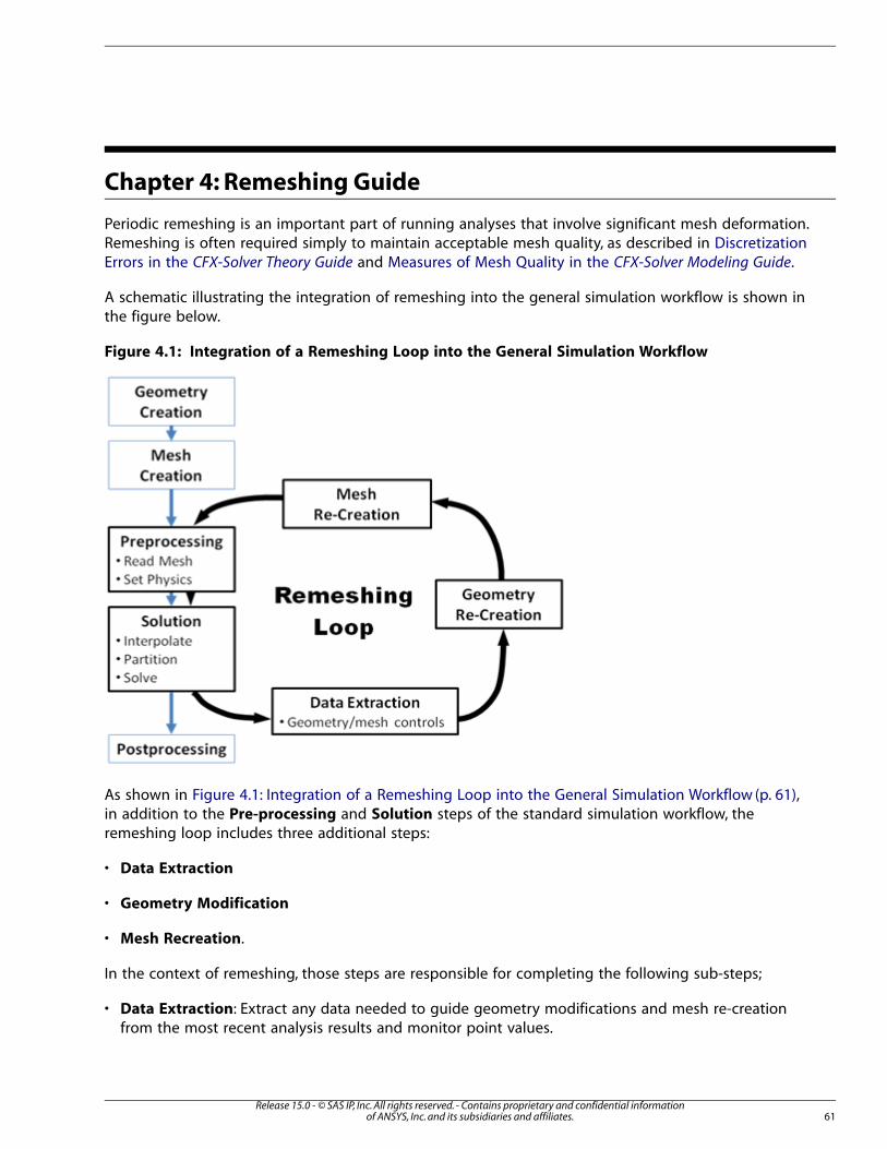
Chapter 4: Remeshing Guide
Periodic remeshing is an important part of running analyses that involve significant mesh deformation.Remeshing is often required simply to maintain acceptable mesh quality, as described in DiscretizationErrors in the CFX-Solver Theory Guide and Measures of Mesh Quality in the CFX-Solver Modeling Guide.
A schematic illustrating the integration of remeshing into the general simulation workflow is shown inthe figure below.
Figure 4.1: Integration of a Remeshing Loop into the General Simulation Workflow
As shown in Figure 4.1: Integration of a Remeshing Loop into the General Simulation Workflow (p. 61),in addition to the Pre-processing and Solution steps of the standard simulation workflow, theremeshing loop includes three additional steps:
• Data Extraction
• Geometry Modification
• Mesh Recreation.
In the context of remeshing, those steps are responsible for completing the following sub-steps;
• Data Extraction: Extract any data needed to guide geometry modifications and mesh re-creationfrom the most recent analysis results and monitor point values.
61Release 15.0 - © SAS IP, Inc. All rights reserved. - Contains proprietary and confidential information
of ANSYS, Inc. and its subsidiaries and affiliates.
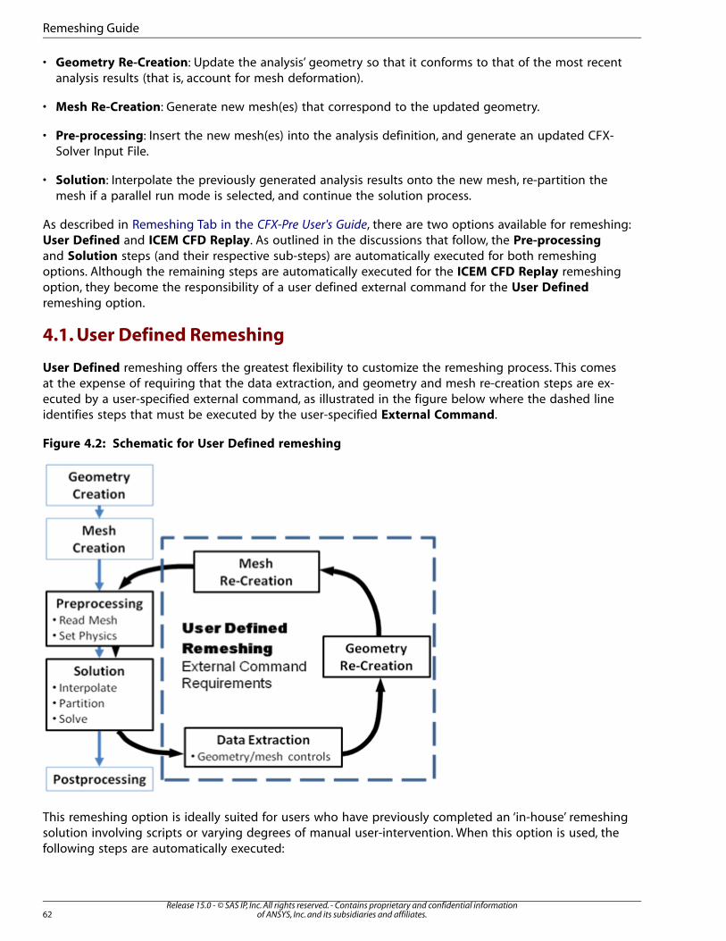
• Geometry Re-Creation: Update the analysis’ geometry so that it conforms to that of the most recentanalysis results (that is, account for mesh deformation).
• Mesh Re-Creation: Generate new mesh(es) that correspond to the updated geometry.
• Pre-processing: Insert the new mesh(es) into the analysis definition, and generate an updated CFX-Solver Input File.
• Solution: Interpolate the previously generated analysis results onto the new mesh, re-partition themesh if a parallel run mode is selected, and continue the solution process.
As described in Remeshing Tab in the CFX-Pre User's Guide, there are two options available for remeshing:User Defined and ICEM CFD Replay. As outlined in the discussions that follow, the Pre-processing
and Solution steps (and their respective sub-steps) are automatically executed for both remeshingoptions. Although the remaining steps are automatically executed for the ICEM CFD Replay remeshingoption, they become the responsibility of a user defined external command for the User Defined
remeshing option.
4.1. User Defined Remeshing
User Defined remeshing offers the greatest flexibility to customize the remeshing process. This comesat the expense of requiring that the data extraction, and geometry and mesh re-creation steps are ex-ecuted by a user-specified external command, as illustrated in the figure below where the dashed lineidentifies steps that must be executed by the user-specified External Command.
Figure 4.2: Schematic for User Defined remeshing
This remeshing option is ideally suited for users who have previously completed an ‘in-house’ remeshingsolution involving scripts or varying degrees of manual user-intervention. When this option is used, thefollowing steps are automatically executed:
Release 15.0 - © SAS IP, Inc. All rights reserved. - Contains proprietary and confidential informationof ANSYS, Inc. and its subsidiaries and affiliates.62
Remeshing Guide
• Run the specified external command to generate a new mesh(es)
• Insert the new mesh(es) into the analysis definition, and generate an updated CFX-Solver Input file
• Interpolate the previously generated analysis results onto the new mesh, re-partition the mesh if aparallel run mode is selected, and continue the solution process.
The following examples outline the use of the User Defined remeshing option:
• Remeshing with Key-Frame Meshes (p. 63)
• Remeshing with Automatic Geometry Extraction (p. 63).
4.1.1. Remeshing with Key-Frame Meshes
In some analyses involving mesh deformation, the motion of various boundaries and sub-domains isknown beforehand. Thus, the iteration or time step number at which unacceptable mesh quality willoccur due to mesh motion is also known. A sequence of ‘key-frame’ meshes (of any mesh file type)corresponding to these instances of poor mesh quality can consequently be generated and appliedduring the analysis.
Once the sequence of key-frame meshes has been generated, they should be placed in a location thatwill be accessible during the analysis’ execution. The analysis definition is then modified to include oneor more control conditions that will interrupt the solver at the iteration or time step at which a key-frame mesh should be inserted. A configuration is subsequently defined (unless this has already beendone), and a remeshing definition is created with the following settings:
• Set Option to User Defined.
• Set the Activation Condition(s) to the previously created interrupt control condition(s).
• Set the Location to the mesh region that will be replaced.
• Set the External Command to the command that will be used to generate the replacement meshfile.
• Set the Replacement File to the name of the file that will be generated by the external command.
The External Command is typically a shell script or batch file that completes the following tasks:
• Determine which key-frame mesh to use. This will require parsing the run’s output file for the iterationor time step number, or the actual simulation time. Output generated from the cfx5mondata ex-ecutable can also be parsed instead of the run’s output file. For details, see Exporting Monitor Datafrom the Command Line in the CFX-Solver Manager User's Guide.
• Copy the key-frame mesh to the path the specified by the Replacement File setting.
4.1.2. Remeshing with Automatic Geometry Extraction
In some analyses involving mesh deformation, the motion of various boundaries and sub-domains isnot known beforehand and the key-frame remeshing strategy presented above is not applicable. Inthese analyses, geometrical information must be extracted from the most recent analysis results andapplied in the remeshing process.
63Release 15.0 - © SAS IP, Inc. All rights reserved. - Contains proprietary and confidential information
of ANSYS, Inc. and its subsidiaries and affiliates.
User Defined Remeshing
In such cases, the analysis definition is modified to include one or more control conditions that will in-terrupt the solver when, for example, mesh quality deteriorates significantly. A configuration is sub-sequently defined (unless this has already been done), and a remeshing definition is created with thefollowing settings:
• Set Option to User Defined.
• Set the Activation Condition(s) to the previously created interrupt control condition(s).
• Set the Location to the mesh region that will be replaced.
• Set the External Command to the command that will be used to generate the replacement meshfile.
• Set the Replacement File to the name of the file that will be generated by the external command.
The External Command is typically a shell script or batch file that completes the following tasks:
• Extract geometry data from the most recent solution of the analysis, and either update or replacethe original geometry. This may be done using mesh-to-geometry conversion tools available in softwaresuch as ANSYS ICEM CFD, or by extracting monitor point data values (for example, the Total CentroidDisplacement variable) using the cfx5mondata executable. For details, see Exporting Monitor Datafrom the Command Line in the CFX-Solver Manager User's Guide.
• Create a replacement mesh file using the updated or newly generated geometry. This may be donein any suitable mesh generation application.
Note that some mesh-to-geometry conversion tools are unable to extract the latest mesh coordinatesfrom the most recent CFX-Solver Results file. If this is the case, then introduce a call to CFX-Pre (withinthe External Command) that executes a session file that simply loads the latest CFX-Solver Results fileand writes a new CFX-Solver Input file. That CFX-Solver Input file will contain the required, latest meshcoordinates.
4.2. ICEM CFD Replay Remeshing
ICEM CFD Replay remeshing provides a highly automated remeshing process that is ideally suited forusers of the ANSYS ICEM CFD mesh generation software and cases that involve translational meshmotion only (that is, no rotation or general deformation). When this option is used, a master replay fileis assembled from other task-oriented replay files and submitted to the ANSYS ICEM CFD mesh gener-ator for batch execution. These replay files are illustrated in the figure below, along with the generalprocess flow for this remeshing option. The dashed line in the figure highlights components of themaster replay file and identifies files and steps that you can modify. Unless otherwise noted, files arecontained in the <CFXROOT>/etc/Remeshing directory.
Release 15.0 - © SAS IP, Inc. All rights reserved. - Contains proprietary and confidential informationof ANSYS, Inc. and its subsidiaries and affiliates.64
Remeshing Guide
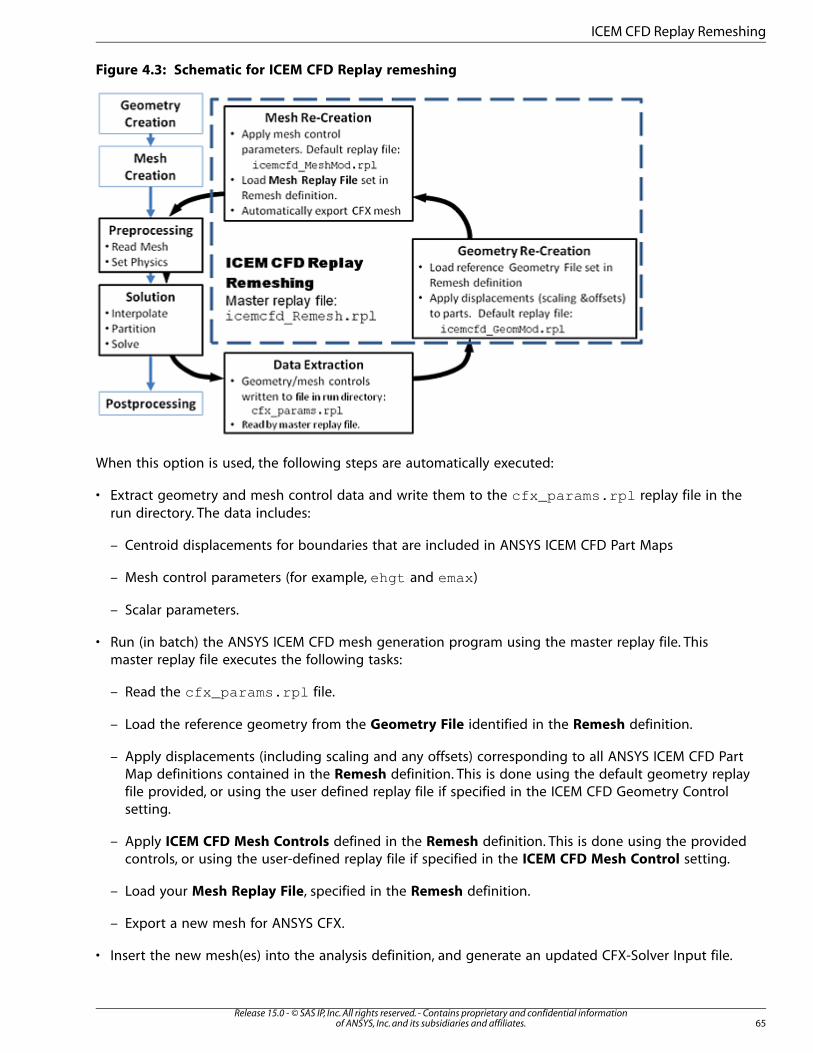
Figure 4.3: Schematic for ICEM CFD Replay remeshing
When this option is used, the following steps are automatically executed:
• Extract geometry and mesh control data and write them to the cfx_params.rpl replay file in therun directory. The data includes:
– Centroid displacements for boundaries that are included in ANSYS ICEM CFD Part Maps
– Mesh control parameters (for example, ehgt and emax)
– Scalar parameters.
• Run (in batch) the ANSYS ICEM CFD mesh generation program using the master replay file. Thismaster replay file executes the following tasks:
– Read the cfx_params.rpl file.
– Load the reference geometry from the Geometry File identified in the Remesh definition.
– Apply displacements (including scaling and any offsets) corresponding to all ANSYS ICEM CFD PartMap definitions contained in the Remesh definition. This is done using the default geometry replayfile provided, or using the user defined replay file if specified in the ICEM CFD Geometry Controlsetting.
– Apply ICEM CFD Mesh Controls defined in the Remesh definition. This is done using the providedcontrols, or using the user-defined replay file if specified in the ICEM CFD Mesh Control setting.
– Load your Mesh Replay File, specified in the Remesh definition.
– Export a new mesh for ANSYS CFX.
• Insert the new mesh(es) into the analysis definition, and generate an updated CFX-Solver Input file.
65Release 15.0 - © SAS IP, Inc. All rights reserved. - Contains proprietary and confidential information
of ANSYS, Inc. and its subsidiaries and affiliates.
ICEM CFD Replay Remeshing
• Interpolate the previously generated analysis results onto the new mesh, re-partition the mesh if aparallel run mode is selected, and continue the solution process.
You must create the reference Geometry File and the Mesh Replay File because these are specific toeach case. However, the generic default replay files (icemcfd_Remesh.rpl , icemcfd_GeomMod.rpl ,and icemcfd_MeshMod.rpl ) used by this option are provided in the <CFXROOT>/etc/Remeshingdirectory. These files may be edited to provide installation-wide changes to the ICEM CFD Replayremeshing behavior. Alternatively, the geometry and mesh modification files may be copied and editedto provide case-specific changes.
Note
As indicated previously, only translational mesh motion is automatically handled by the ICEMCFD Replay remeshing option. This is accomplished by applying the displacements of centroidsof boundaries in the ANSYS CFX analysis definition to parts in the ANSYS ICEM CFD geometry.All other mesh motion (such as rotation about the centroid or another point, or general de-formation) will not be applied, and an inconsistency in the analysis geometry before andafter remeshing will be introduced.
4.2.1. Steps to Set Up a Simulation Using ICEM CFD Replay Remeshing
The following discussion presents the three general steps required to set up a simulation using theICEM CFD Replay remeshing option.
The first step involves creating the reference Geometry File within the ANSYS ICEM CFD environment.If the geometry was not created within that environment, use one of the File > Import Geometry optionsin the ANSYS ICEM CFD environment. At this point, ensure that all required Parts (or Families) are definedand named so that they can be referenced when completing the ICEM CFD Replay remeshing definitionlater in CFX-Pre. Finally, store the geometry in the ICEM CFD native geometry file format (namely, a.tin file).
The second step involves generating the Mesh Replay File, again, from within the ANSYS ICEM CFDenvironment. Start with the previously created geometry loaded, and work sequentially through themesh generation process until acceptable mesh controls have been specified. This may require finetuning, which will involve the regeneration of your mesh after moving the geometry through its expectedrange of motion. Once you are satisfied with the mesh control settings, purge the last mesh using File
> Mesh > Close Mesh, and reload the original reference geometry. Complete the following tasks togenerate the required Mesh Replay File:
1. Use File > Replay Scripts > Replay Control to begin recording the commands for the Mesh Replay
File. The Replay Control dialog box is displayed.
2. Revisit all of the mesh related tabs and settings used to generate the mesh, clicking either the Apply
or OK to commit the settings into the Replay Control panel.
3. Generate the mesh.
4. In the Replay Control panel, clear the Record (after current) toggle and select Save to write the settingsto replay file.
You may also want to export the mesh that was (re)generated for use in the simulation definition (asin the next step).
Release 15.0 - © SAS IP, Inc. All rights reserved. - Contains proprietary and confidential informationof ANSYS, Inc. and its subsidiaries and affiliates.66
Remeshing Guide
The third step involves defining the simulation within CFX-Pre. Complete the following tasks to preparethe simulation:
1. Start a new simulation and import the (previously generated) mesh.
2. Define expressions for the motion of the geometry (for example, see the expressions for the ballmovement in Modeling a Ball Check Valve using Mesh Deformation and the CFX Rigid Body Solver inthe CFX Tutorials).
Note
See also the discussion in Mesh Re-Initialization During Remeshing (p. 68).
3. Define the flow analysis including the definition of one or more solver interrupt controls, as describedin Interrupt Control in the CFX-Pre User's Guide, to identify the condition(s) under which solver executionwill be interrupted.
4. Define a configuration and complete the ICEM CFD Replay remeshing setup as described in ANSYS ICEMCFD Replay Remeshing in the CFX-Pre User's Guide. The Geometry File and Mesh Replay File createdabove are referenced here. Note also, that references to one or more of the previously defined solverinterrupt control conditions are required to activate remeshing.
5. Complete any execution controls for the simulation and either start the solver or write the CFX-SolverInput file for later use.
4.3. Directory Structure and Files Used During Remeshing
CFX-Solver runs that include remeshing will have a slightly non-standard directory structure during ex-ecution. For example, using a CFX-Solver input file named case.def , a directory structure similar tothe following will exist just after solution execution is interrupted and the second instance of remeshingbegins:
case.def case_001/ 1_full.trn 0_full.trn 2_full.trn 3_oldmesh.res 3_remesh.out case_001.dir/ 3_full.trn 4_full.trn res mon
The first instance of remeshing occurred when the solver was interrupted after the third time step.Following this instance of remeshing, all CFX-Solver Results files (such as transient, backup, andremeshing) contained in the run directory, case_001.dir , were moved into the final solution directory,case_001 . The results file written when the solver was interrupted before remeshing was renamed to3_oldmesh.res . Any text output to the console window during remeshing was redirected to the filenamed 3_remesh.out , which is also placed in the final solution directory.
The second, and currently running, instance of remeshing began when the solver was interrupted afterthe fifth time step. The results file written by the solver still has the generic name, res , and monitordata (contained in the mon file) has not yet been inserted into the results file.
67Release 15.0 - © SAS IP, Inc. All rights reserved. - Contains proprietary and confidential information
of ANSYS, Inc. and its subsidiaries and affiliates.
Directory Structure and Files Used During Remeshing
Just after inserting the new mesh(es) into the analysis definition, the files contained in the final solutionand run directories change slightly. The results and console output files are renamed (to5_oldmesh.res and 5_remesh.out , respectively) and moved from the run directory into the finalsolution directory. An automatically generated session file, meshUpdate.pre , is used by CFX-Pre togenerate the updated the solver input file, 5_newmesh.def , and each of these files are present in therun directory. These files are, however, replaced or removed during the next instance of remeshing orwhen the analysis ends and the run directory is deleted.
4.4. Additional Considerations
This section discusses additional considerations for remeshing.4.4.1. Mesh Re-Initialization During Remeshing4.4.2. Software License Handling4.4.3. Results File Option
4.4.1. Mesh Re-Initialization During Remeshing
The following points are important to note during remeshing:
• The total mesh displacement variable is relative to a specific mesh topology. Because the mesh topo-logy changes, this variable is reset each time remeshing occurs.
• The new variable called total centroid displacement tracks the displacement of eachboundary’s centroid since the beginning of the analysis (that is, relative to the original mesh).
• The specified displacement based mesh motion is relative to the initial mesh and must therefore includean offset to account for mesh re-initialization. The Mesh Initialisation Time variable corres-ponds to the time at which mesh re-initialization last occurred. This can be used to evaluate the re-quired offset for time varying mesh displacement.
An example of the expressions used to evaluate an applied displacement that includes the requiredoffset to account for mesh re-initialization is given below. In this example, the applied displacement isevaluated as the desired displacement minus the value of the desired displacement at the MeshInitialisation Time .
Disp Desired = 1[m]*0.5*(1-cos(2.[s^-1]*pi*t))Disp Mesh ReInit = 1[m]*0.5*(1-cos(2.[s^-1]*pi*Mesh Initialisation Time ))Disp Applied = Disp Desired - Disp Mesh ReInit
4.4.2. Software License Handling
Several software components (for example, CFX-Pre, the CFX-Solver, ANSYS ICEM CFD, and so on) areused while executing steps in the overall remeshing process. Rather than holding all of these licensesfor the entire duration of the analysis, they are only ‘checked out’ as required. Although this frees upthe licenses for other users when remeshing is not executing, it also introduces the possibility that re-quired licenses are not available when they are needed for remeshing.
This model for software license handling may cause problems in multi-user environments, but work isunderway to provide a broader range of handling options for future releases.
4.4.3. Results File Option
In order for remeshing to proceed, results files must be of type Standard , Essential , or Refiner .
Release 15.0 - © SAS IP, Inc. All rights reserved. - Contains proprietary and confidential informationof ANSYS, Inc. and its subsidiaries and affiliates.68
Remeshing Guide
Chapter 5: Reference Guide for Mesh Deformation and
Fluid-Structure Interaction
This guide is part of a series that provides advice for using CFX in specific engineering application areas.It is aimed at users with little or moderate experience using CFX for applications involving Mesh Deform-ation and/or Fluid Structure Interaction.
This guide describes:5.1. Mesh Deformation5.2. Fluid Structure Interaction
5.1. Mesh Deformation
Mesh deformation is an important part of executing simulations with changing domain geometry. InCFX, this capability is available in fluid and solid domains. Motion can be specified on selected regionsvia CEL or an external solver coupling (for example, ANSYS Multi-field MFX), or on all nodes in an entiredomain via a user-Fortran junction box routine.
5.1.1. Mesh Folding: Negative Sector and Element Volumes
It is not uncommon for the mesh to become folded (or tangled) during the mesh deformation process.When this occurs, a message indicating the existence and location of either negative sector volumesor negative (that is, topologically invalid) elements is written to the simulation output file. Notificationof negative sector volumes highlights the existence of non-convex mesh elements that still have apositive volume. Although the existence of negative sector volumes is not a fatal condition, it does in-dicate that:
• Mesh elements are only barely positive
• Further mesh deformation is likely to yield elements with negative volumes, which is a fatal condition
Some of the most common causes for mesh folding during deformation are identified in the followingsections.
5.1.2. Applying Large Displacements Gradually
In many simulations that require mesh deformation, the motion is known a priori. In these cases, themotion can be applied gradually, by relating it to the iteration or timestep counters, to reduce thelikelihood of mesh folding. Mesh folding is often avoided with this strategy because the mesh displace-ment equations are assembled using the updated meshes from each deformation step (that is, outeriteration or timestep). In general, the desired total mesh deformation should be split up so that regionswhere motion is specified move through less than approximately 5 adjacent elements per step.
In some simulations, the motion is not known a priori. Fluid Structure Interaction is an excellent exampleof this. In these cases, mechanisms available for under-relaxing the displacements applied per deform-ation step should be used. For details, see Solver Controls, External Coupling Tab in the CFX-Solver
Modeling Guide.
69Release 15.0 - © SAS IP, Inc. All rights reserved. - Contains proprietary and confidential information
of ANSYS, Inc. and its subsidiaries and affiliates.
5.1.3. Consistency of Mesh Motion Specifications
Mesh motion options such as Specified Displacement may be applied on multiple boundaryand subdomain regions. Because the specified motion is applied directly to mesh nodes, rather thancontrol volume integration points, care is required to ensure that motion specified on adjacent regionsis self-consistent. For example, the motion specified on one moving wall should be reduced to zero forany nodes that are shared with another stationary wall. If this is not done, then the motion applied tothe shared nodes will be either the moving or stationary condition, depending on which was appliedlast during the equation assembly process.
Folded meshes often result from the application of inconsistent motion specifications.
5.1.4. Solving the Mesh Displacement Equations and Updating Mesh Coordin-
ates
During each outer iteration or timestep, the mesh displacement equations are solved to the specifiedconvergence level and the resulting displacements are applied to update the mesh coordinates. Thisoccurs before proceeding to solve the general transport (for example, hydrodynamics, turbulence, etc.)equations.
Unlike other equation classes, the convergence level (that is, controls and criteria) applied to meshdisplacement equations is unaffected by changes made to the basic settings for all other equations.The default convergence controls and criteria for the mesh displacement equation are tabulated below,and are changed by visiting the Mesh Displacement entry in the Equation Class Settings tab underSolver Control.
ValueSetting
5Maximum Number of CoefficientLoops
1Minimum Number of CoefficientLoops
RMSResidual Type
1.0E-4Residual Target
Mesh folding occurs and is detected when the displacements are used to update the mesh coordinates.Folded meshes can occur if the displacement equations are incompletely solved. In this case, the uncon-verged displacement solution field does not vary smoothly enough to ensure that adjacent mesh nodesmove by similar amounts.
5.1.5. Mesh Displacement Diffusion Scheme
A number of numerical schemes are available for the solution of the mesh displacement diffusionequation. In many cases the default scheme is appropriate, but in some situations mesh folding can beavoided and improved mesh quality can be obtained by using a different scheme. The expert parametermeshdisp diffusion scheme controls which numerical scheme is used. For details, see Discretiz-ation Parameters. Setting meshdisp diffusion scheme to 3 can be helpful if the mesh folds un-expectedly at sharp corners or if uniform mesh deformation is expected but non-uniform deformationis observed. The figures below show an example of using different mesh displacement diffusion schemes.
Release 15.0 - © SAS IP, Inc. All rights reserved. - Contains proprietary and confidential informationof ANSYS, Inc. and its subsidiaries and affiliates.70
Reference Guide for Mesh Deformation and Fluid-Structure Interaction
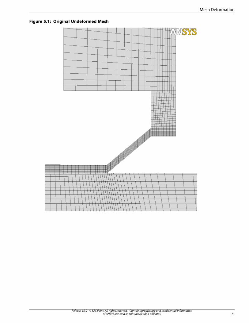
Figure 5.1: Original Undeformed Mesh
71Release 15.0 - © SAS IP, Inc. All rights reserved. - Contains proprietary and confidential information
of ANSYS, Inc. and its subsidiaries and affiliates.
Mesh Deformation
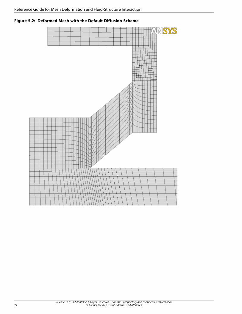
Figure 5.2: Deformed Mesh with the Default Diffusion Scheme
Release 15.0 - © SAS IP, Inc. All rights reserved. - Contains proprietary and confidential informationof ANSYS, Inc. and its subsidiaries and affiliates.72
Reference Guide for Mesh Deformation and Fluid-Structure Interaction
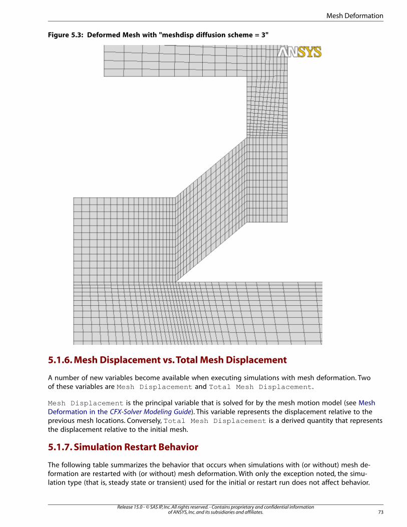
Figure 5.3: Deformed Mesh with "meshdisp diffusion scheme = 3"
5.1.6. Mesh Displacement vs. Total Mesh Displacement
A number of new variables become available when executing simulations with mesh deformation. Twoof these variables are Mesh Displacement and Total Mesh Displacement .
Mesh Displacement is the principal variable that is solved for by the mesh motion model (see MeshDeformation in the CFX-Solver Modeling Guide). This variable represents the displacement relative to theprevious mesh locations. Conversely, Total Mesh Displacement is a derived quantity that representsthe displacement relative to the initial mesh.
5.1.7. Simulation Restart Behavior
The following table summarizes the behavior that occurs when simulations with (or without) mesh de-formation are restarted with (or without) mesh deformation. With only the exception noted, the simu-lation type (that is, steady state or transient) used for the initial or restart run does not affect behavior.
73Release 15.0 - © SAS IP, Inc. All rights reserved. - Contains proprietary and confidential information
of ANSYS, Inc. and its subsidiaries and affiliates.
Mesh Deformation
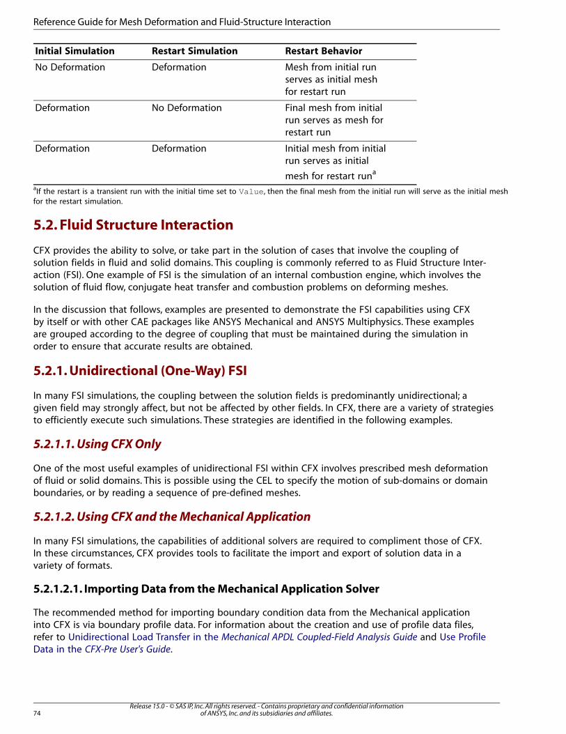
Restart BehaviorRestart SimulationInitial Simulation
Mesh from initial runserves as initial meshfor restart run
DeformationNo Deformation
Final mesh from initialrun serves as mesh forrestart run
No DeformationDeformation
Initial mesh from initialrun serves as initial
mesh for restart runa
DeformationDeformation
aIf the restart is a transient run with the initial time set to Value , then the final mesh from the initial run will serve as the initial meshfor the restart simulation.
5.2. Fluid Structure Interaction
CFX provides the ability to solve, or take part in the solution of cases that involve the coupling ofsolution fields in fluid and solid domains. This coupling is commonly referred to as Fluid Structure Inter-action (FSI). One example of FSI is the simulation of an internal combustion engine, which involves thesolution of fluid flow, conjugate heat transfer and combustion problems on deforming meshes.
In the discussion that follows, examples are presented to demonstrate the FSI capabilities using CFXby itself or with other CAE packages like ANSYS Mechanical and ANSYS Multiphysics. These examplesare grouped according to the degree of coupling that must be maintained during the simulation inorder to ensure that accurate results are obtained.
5.2.1. Unidirectional (One-Way) FSI
In many FSI simulations, the coupling between the solution fields is predominantly unidirectional; agiven field may strongly affect, but not be affected by other fields. In CFX, there are a variety of strategiesto efficiently execute such simulations. These strategies are identified in the following examples.
5.2.1.1. Using CFX Only
One of the most useful examples of unidirectional FSI within CFX involves prescribed mesh deformationof fluid or solid domains. This is possible using the CEL to specify the motion of sub-domains or domainboundaries, or by reading a sequence of pre-defined meshes.
5.2.1.2. Using CFX and the Mechanical Application
In many FSI simulations, the capabilities of additional solvers are required to compliment those of CFX.In these circumstances, CFX provides tools to facilitate the import and export of solution data in avariety of formats.
5.2.1.2.1. Importing Data from the Mechanical Application Solver
The recommended method for importing boundary condition data from the Mechanical applicationinto CFX is via boundary profile data. For information about the creation and use of profile data files,refer to Unidirectional Load Transfer in the Mechanical APDL Coupled-Field Analysis Guide and Use ProfileData in the CFX-Pre User's Guide.
Release 15.0 - © SAS IP, Inc. All rights reserved. - Contains proprietary and confidential informationof ANSYS, Inc. and its subsidiaries and affiliates.74
Reference Guide for Mesh Deformation and Fluid-Structure Interaction
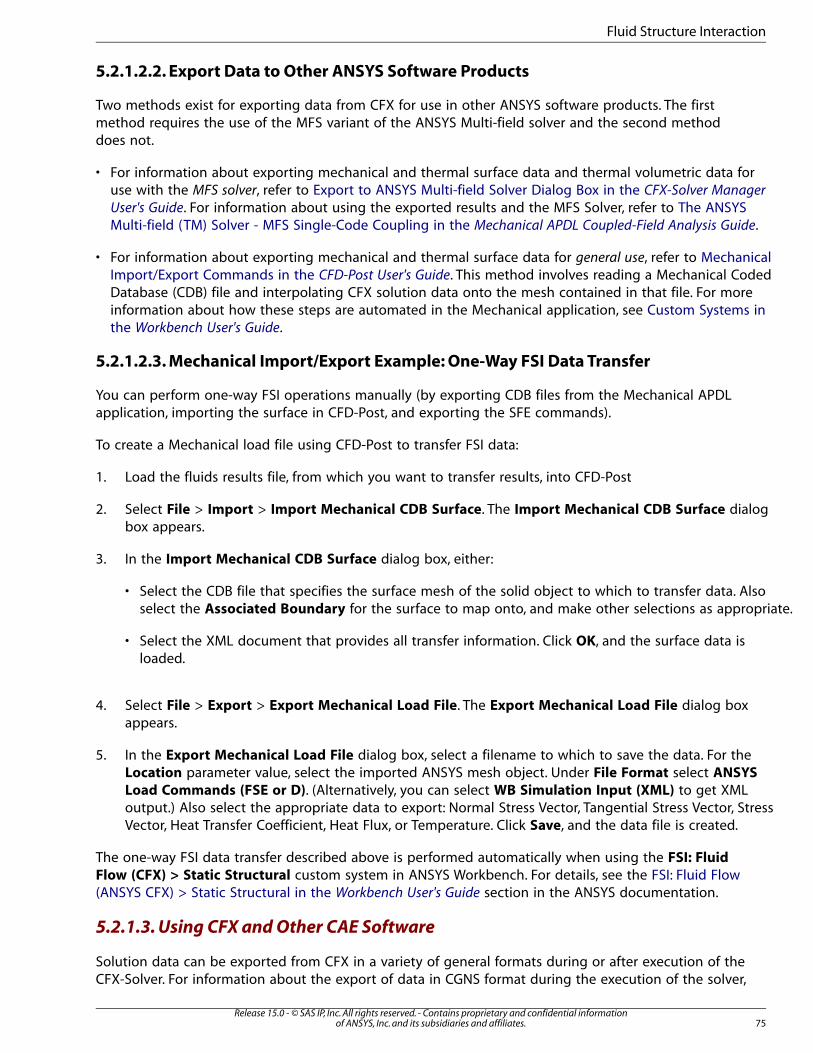
5.2.1.2.2. Export Data to Other ANSYS Software Products
Two methods exist for exporting data from CFX for use in other ANSYS software products. The firstmethod requires the use of the MFS variant of the ANSYS Multi-field solver and the second methoddoes not.
• For information about exporting mechanical and thermal surface data and thermal volumetric data foruse with the MFS solver, refer to Export to ANSYS Multi-field Solver Dialog Box in the CFX-Solver Manager
User's Guide. For information about using the exported results and the MFS Solver, refer to The ANSYSMulti-field (TM) Solver - MFS Single-Code Coupling in the Mechanical APDL Coupled-Field Analysis Guide.
• For information about exporting mechanical and thermal surface data for general use, refer to MechanicalImport/Export Commands in the CFD-Post User's Guide. This method involves reading a Mechanical CodedDatabase (CDB) file and interpolating CFX solution data onto the mesh contained in that file. For moreinformation about how these steps are automated in the Mechanical application, see Custom Systems inthe Workbench User's Guide.
5.2.1.2.3. Mechanical Import/Export Example: One-Way FSI Data Transfer
You can perform one-way FSI operations manually (by exporting CDB files from the Mechanical APDLapplication, importing the surface in CFD-Post, and exporting the SFE commands).
To create a Mechanical load file using CFD-Post to transfer FSI data:
1. Load the fluids results file, from which you want to transfer results, into CFD-Post
2. Select File > Import > Import Mechanical CDB Surface. The Import Mechanical CDB Surface dialogbox appears.
3. In the Import Mechanical CDB Surface dialog box, either:
• Select the CDB file that specifies the surface mesh of the solid object to which to transfer data. Alsoselect the Associated Boundary for the surface to map onto, and make other selections as appropriate.
• Select the XML document that provides all transfer information. Click OK, and the surface data isloaded.
4. Select File > Export > Export Mechanical Load File. The Export Mechanical Load File dialog boxappears.
5. In the Export Mechanical Load File dialog box, select a filename to which to save the data. For theLocation parameter value, select the imported ANSYS mesh object. Under File Format select ANSYS
Load Commands (FSE or D). (Alternatively, you can select WB Simulation Input (XML) to get XMLoutput.) Also select the appropriate data to export: Normal Stress Vector, Tangential Stress Vector, StressVector, Heat Transfer Coefficient, Heat Flux, or Temperature. Click Save, and the data file is created.
The one-way FSI data transfer described above is performed automatically when using the FSI: Fluid
Flow (CFX) > Static Structural custom system in ANSYS Workbench. For details, see the FSI: Fluid Flow(ANSYS CFX) > Static Structural in the Workbench User's Guide section in the ANSYS documentation.
5.2.1.3. Using CFX and Other CAE Software
Solution data can be exported from CFX in a variety of general formats during or after execution of theCFX-Solver. For information about the export of data in CGNS format during the execution of the solver,
75Release 15.0 - © SAS IP, Inc. All rights reserved. - Contains proprietary and confidential information
of ANSYS, Inc. and its subsidiaries and affiliates.
Fluid Structure Interaction
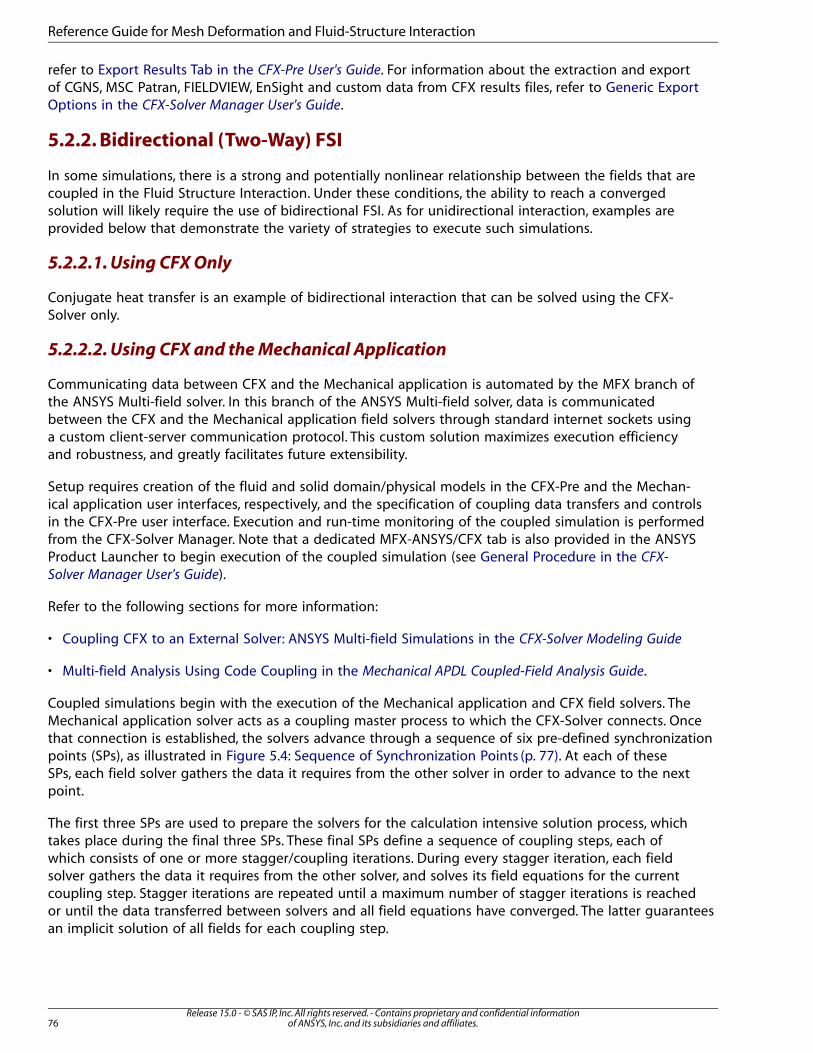
refer to Export Results Tab in the CFX-Pre User's Guide. For information about the extraction and exportof CGNS, MSC Patran, FIELDVIEW, EnSight and custom data from CFX results files, refer to Generic ExportOptions in the CFX-Solver Manager User's Guide.
5.2.2. Bidirectional (Two-Way) FSI
In some simulations, there is a strong and potentially nonlinear relationship between the fields that arecoupled in the Fluid Structure Interaction. Under these conditions, the ability to reach a convergedsolution will likely require the use of bidirectional FSI. As for unidirectional interaction, examples areprovided below that demonstrate the variety of strategies to execute such simulations.
5.2.2.1. Using CFX Only
Conjugate heat transfer is an example of bidirectional interaction that can be solved using the CFX-Solver only.
5.2.2.2. Using CFX and the Mechanical Application
Communicating data between CFX and the Mechanical application is automated by the MFX branch ofthe ANSYS Multi-field solver. In this branch of the ANSYS Multi-field solver, data is communicatedbetween the CFX and the Mechanical application field solvers through standard internet sockets usinga custom client-server communication protocol. This custom solution maximizes execution efficiencyand robustness, and greatly facilitates future extensibility.
Setup requires creation of the fluid and solid domain/physical models in the CFX-Pre and the Mechan-ical application user interfaces, respectively, and the specification of coupling data transfers and controlsin the CFX-Pre user interface. Execution and run-time monitoring of the coupled simulation is performedfrom the CFX-Solver Manager. Note that a dedicated MFX-ANSYS/CFX tab is also provided in the ANSYSProduct Launcher to begin execution of the coupled simulation (see General Procedure in the CFX-
Solver Manager User's Guide).
Refer to the following sections for more information:
• Coupling CFX to an External Solver: ANSYS Multi-field Simulations in the CFX-Solver Modeling Guide
• Multi-field Analysis Using Code Coupling in the Mechanical APDL Coupled-Field Analysis Guide.
Coupled simulations begin with the execution of the Mechanical application and CFX field solvers. TheMechanical application solver acts as a coupling master process to which the CFX-Solver connects. Oncethat connection is established, the solvers advance through a sequence of six pre-defined synchronizationpoints (SPs), as illustrated in Figure 5.4: Sequence of Synchronization Points (p. 77). At each of theseSPs, each field solver gathers the data it requires from the other solver in order to advance to the nextpoint.
The first three SPs are used to prepare the solvers for the calculation intensive solution process, whichtakes place during the final three SPs. These final SPs define a sequence of coupling steps, each ofwhich consists of one or more stagger/coupling iterations. During every stagger iteration, each fieldsolver gathers the data it requires from the other solver, and solves its field equations for the currentcoupling step. Stagger iterations are repeated until a maximum number of stagger iterations is reachedor until the data transferred between solvers and all field equations have converged. The latter guaranteesan implicit solution of all fields for each coupling step.
Release 15.0 - © SAS IP, Inc. All rights reserved. - Contains proprietary and confidential informationof ANSYS, Inc. and its subsidiaries and affiliates.76
Reference Guide for Mesh Deformation and Fluid-Structure Interaction
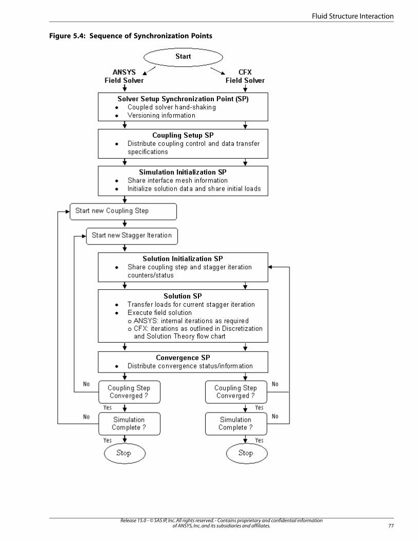
Figure 5.4: Sequence of Synchronization Points
77Release 15.0 - © SAS IP, Inc. All rights reserved. - Contains proprietary and confidential information
of ANSYS, Inc. and its subsidiaries and affiliates.
Fluid Structure Interaction

5.2.2.3. Using CFX and Other CAE Software
Third party code-coupling software or proprietary interfaces provided by the CAE software vendors canalso be used in conjunction with CFX. Contact those software providers and your CFX service represent-ative for more information.
Release 15.0 - © SAS IP, Inc. All rights reserved. - Contains proprietary and confidential informationof ANSYS, Inc. and its subsidiaries and affiliates.78
Reference Guide for Mesh Deformation and Fluid-Structure Interaction

Chapter 6: CFX Best Practices Guide for Numerical Accuracy
This guide provides best practice guidelines for Computational Fluid Dynamics (CFD) simulation anddocumentation of the verification, validation, and demonstration test cases. It describes:
• An Approach to Error Identification, Estimation and Validation (p. 79)
• Definition of Errors in CFD Simulations (p. 80)
• General Best Practice Guidelines (p. 89)
• Selection and Evaluation of Experimental Data (p. 100)
This guide is aimed at users who have moderate or little experience using ANSYS CFX. It is part of aseries that provides advice for using ANSYS CFX in specific engineering application areas. The currentguidelines are adapted from Best Practice Guidelines developed for the nuclear reactor safety applications[143 (p. 344)].
6.1. An Approach to Error Identification, Estimation and Validation
An evaluation of CFD capabilities has to ensure that the different types of errors are identified and, asfar as possible, treated separately. It is known from single-phase studies that the quantification anddocumentation of modeling errors (as in turbulence models, for example) can be achieved only if theother major sources of errors are reduced below an “acceptable” level. In an ideal world, this wouldmean, among other demands, that solutions are provided for grids and with timesteps that are fineenough so that numerical errors can be neglected. This is not a trivial task and the separation of errorscannot always be achieved. These difficulties will be greatly increased by the inclusion of multi-phasephysics and unsteady effects. Nevertheless, the worst strategy would be to avoid the subject and toprovide solutions on a single grid, with a single timestep, and with other uncertainties in initial conditionsand boundary conditions not evaluated. This would result in solutions that would be of little use forthe validation goals.
An essential quantity in the quality assurance procedure is the definition of target variables. They willmainly be scalar (integral) quantities (for instance, forces, heat transfer rates, and maximum temperature)or one-dimensional distributions, such as the wall heat transfer along a certain line. Convergencestudies can be based on these variables without a reference to the grid used in the simulation. Theycan also be used for an asymptotic evaluation of convergence on unstructured meshes. Even moreimportant, these quantities are of immediate meaning to engineers and enable them to understandthe uncertainty from a physical standpoint. A danger of integral or local scalar quantities is that theymight not be sensitive enough to detect local changes in the solutions under grid refinement. Thisshould be kept in mind during the analysis.
In order to tackle the problem, it is necessary to first define the different type of errors that can impacta CFD simulation. It is then required that you list the most promising strategies in order to reduce oravoid these errors. Based on these strategies, procedures have to be defined that can be used for thetest case simulations.
79Release 15.0 - © SAS IP, Inc. All rights reserved. - Contains proprietary and confidential information
of ANSYS, Inc. and its subsidiaries and affiliates.

It might be not possible to rigorously perform the error estimation and reduction procedures describedin the following sections for the complex demonstration cases. However, the best attempt should bemade to follow the principal ideas and to avoid single grid solutions without sensitivity studies. Forthese cases, it is even more important to follow a stringent documentation procedure and to list thepossible deficiencies and uncertainties in the simulations.
The strategies for the reduction and evaluation of numerical errors have been developed for single-phase flows. There is no principal difference between the single- and multi-phase flow formulations.They are both based on (ensemble) averaged equations, and are mathematically similar. From a physicalstandpoint, there are however significant additional challenges due to the presence of the differentphases, besides the obviously higher demands on model formulation. One of the additional complicationlies in the presence of sharp interfaces between the phases, which require a higher degree of grid res-olution than usually necessary for single-phase flows. In addition, multi-phase flows have a higher affinityto physical instabilities that might be suppressed on coarse grids, but appear under grid refinement.(This effect is sometimes also observed in single-phase flows. An example is the blunt trailing edge ofan airfoil, where extreme grid refinement will eventually capture the vortex shedding of the mixinglayer). It is to be kept in mind that the brute application of procedures might not lead to the desiredresults. Also in these cases, the spirit behind the guidelines should be followed and carried as far aspossible.
Validation studies have to be based on experimental data. These data can introduce significant errorsinto the comparison. It is therefore required to select the project test cases with attention to potentialerror sources and experimental uncertainties. Definitions on the different types of test cases as well ason the requirements for the project are given in Selection and Evaluation of Experimental Data (p. 100).
6.2. Definition of Errors in CFD Simulations
CFD simulations have the following potential sources for errors or uncertainties:
• Numerical Errors (p. 81)
Numerical errors result from the differences between the exact equations and the discretized equationssolved by the CFD code. For consistent discretization schemes, these errors can be reduced by anincreased spatial grid density and/or by smaller timesteps.
• Modeling Errors (p. 87)
Modeling errors result from the necessity to describe flow phenomena such as turbulence, combustion,and multi-phase flows by empirical models. For turbulent flows, the necessity for using empirical
models derives from the excessive computational effort to solve the exact equations1 with a Direct
Numerical Simulation (DNS) approach. Turbulence models are therefore required to bridge the gapbetween the real flow and the statistically averaged equations. Other examples are combustionmodels and models for interpenetrating continua, for example, two-fluid models for two-phase flows.
• User Errors (p. 88)
User errors result from incorrect use of CFD software and are usually a result of insufficient expertiseby the CFD user. Errors can be reduced or avoided by additional training and experience in combin-ation with high-quality project management and by provision and use of Best Practice Guidelinesand associated checklists.
• Application Uncertainties (p. 88)
1The Navier-Stokes equations for single-phase, Newtonian fluids
Release 15.0 - © SAS IP, Inc. All rights reserved. - Contains proprietary and confidential informationof ANSYS, Inc. and its subsidiaries and affiliates.80
CFX Best Practices Guide for Numerical Accuracy
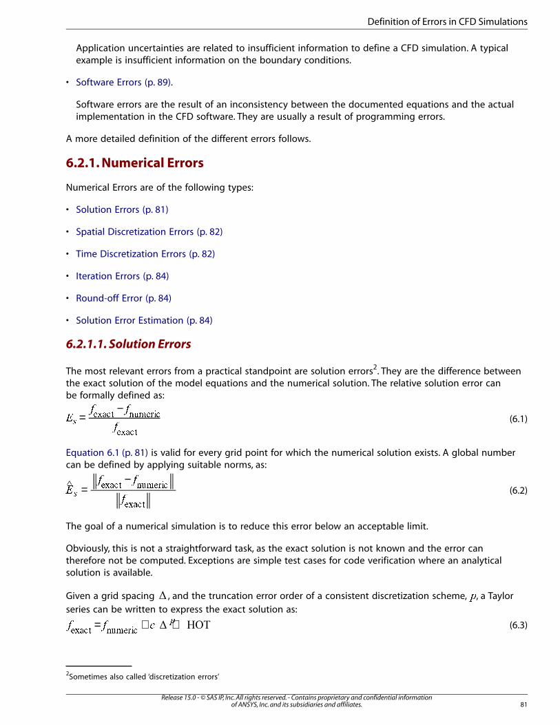
Application uncertainties are related to insufficient information to define a CFD simulation. A typicalexample is insufficient information on the boundary conditions.
• Software Errors (p. 89).
Software errors are the result of an inconsistency between the documented equations and the actualimplementation in the CFD software. They are usually a result of programming errors.
A more detailed definition of the different errors follows.
6.2.1. Numerical Errors
Numerical Errors are of the following types:
• Solution Errors (p. 81)
• Spatial Discretization Errors (p. 82)
• Time Discretization Errors (p. 82)
• Iteration Errors (p. 84)
• Round-off Error (p. 84)
• Solution Error Estimation (p. 84)
6.2.1.1. Solution Errors
The most relevant errors from a practical standpoint are solution errors2. They are the difference betweenthe exact solution of the model equations and the numerical solution. The relative solution error canbe formally defined as:
(6.1)=−
�� �
��
����� �����
�����
Equation 6.1 (p. 81) is valid for every grid point for which the numerical solution exists. A global numbercan be defined by applying suitable norms, as:
(6.2)=−
� �
��
����� �������
�����
The goal of a numerical simulation is to reduce this error below an acceptable limit.
Obviously, this is not a straightforward task, as the exact solution is not known and the error cantherefore not be computed. Exceptions are simple test cases for code verification where an analyticalsolution is available.
Given a grid spacing , and the truncation error order of a consistent discretization scheme, �, a Taylorseries can be written to express the exact solution as:
(6.3)= + +� � ��
�� !" #$%�&'!
2Sometimes also called ‘discretization errors’
81Release 15.0 - © SAS IP, Inc. All rights reserved. - Contains proprietary and confidential information
of ANSYS, Inc. and its subsidiaries and affiliates.
Definition of Errors in CFD Simulations
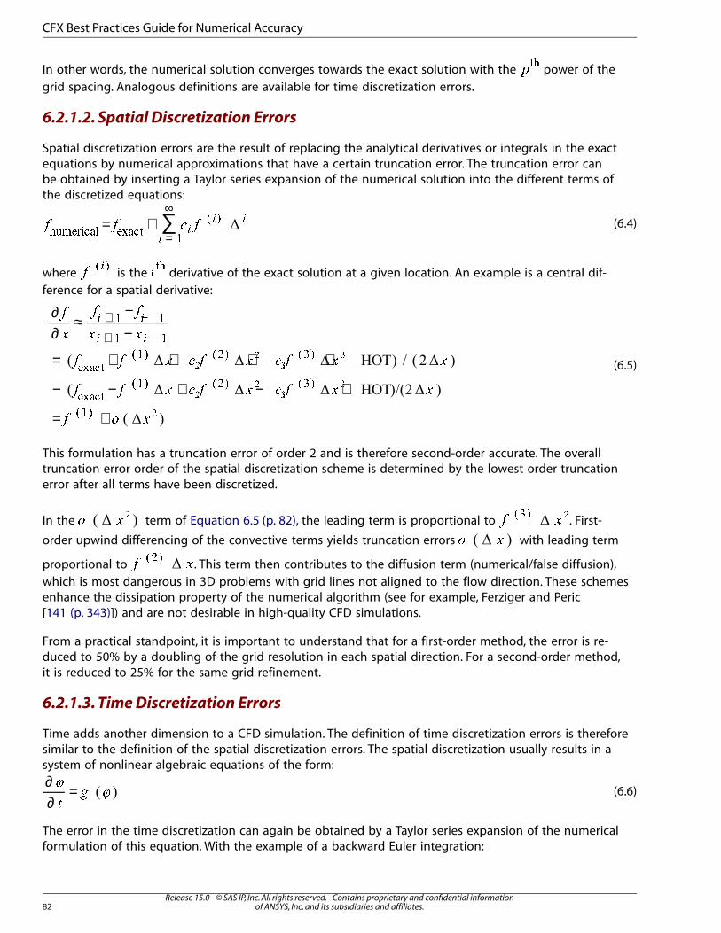
In other words, the numerical solution converges towards the exact solution with the ���
power of thegrid spacing. Analogous definitions are available for time discretization errors.
6.2.1.2. Spatial Discretization Errors
Spatial discretization errors are the result of replacing the analytical derivatives or integrals in the exactequations by numerical approximations that have a certain truncation error. The truncation error canbe obtained by inserting a Taylor series expansion of the numerical solution into the different terms ofthe discretized equations:
(6.4)∑= +=
∞� � � �
��
� �
����� � � ���
� �
where ��� �
is the ���
derivative of the exact solution at a given location. An example is a central dif-ference for a spatial derivative:
(6.5)
∂∂
≈−−
= + + + +
− − + − +
= +
+ −
+ −
�
�
� �
� �
� � � � � � � � � �
� � � � � � � � � �
� � �
� �
� �
!"#$%
& ' &(' &)'
!"#$%
& ' &(' &)'
& '
* +
* +
, -
, -
,
This formulation has a truncation error of order 2 and is therefore second-order accurate. The overalltruncation error order of the spatial discretization scheme is determined by the lowest order truncationerror after all terms have been discretized.
In the . /0
term of Equation 6.5 (p. 82), the leading term is proportional to 1 2345 6
. First-
order upwind differencing of the convective terms yields truncation errors 7 8 with leading term
proportional to 9 :;<=
. This term then contributes to the diffusion term (numerical/false diffusion),which is most dangerous in 3D problems with grid lines not aligned to the flow direction. These schemesenhance the dissipation property of the numerical algorithm (see for example, Ferziger and Peric[141 (p. 343)]) and are not desirable in high-quality CFD simulations.
From a practical standpoint, it is important to understand that for a first-order method, the error is re-duced to 50% by a doubling of the grid resolution in each spatial direction. For a second-order method,it is reduced to 25% for the same grid refinement.
6.2.1.3. Time Discretization Errors
Time adds another dimension to a CFD simulation. The definition of time discretization errors is thereforesimilar to the definition of the spatial discretization errors. The spatial discretization usually results in asystem of nonlinear algebraic equations of the form:
(6.6)∂∂
=>
?@ >
The error in the time discretization can again be obtained by a Taylor series expansion of the numericalformulation of this equation. With the example of a backward Euler integration:
Release 15.0 - © SAS IP, Inc. All rights reserved. - Contains proprietary and confidential informationof ANSYS, Inc. and its subsidiaries and affiliates.82
CFX Best Practices Guide for Numerical Accuracy
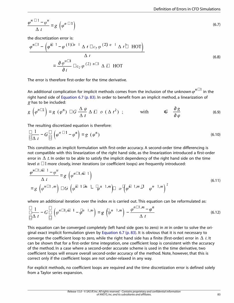
(6.7)− =+
+� �
�� �
� ��
��
the discretization error is:
(6.8)
− − + +
= ∂∂
+ +
+ + + +
++
� � � � � � �
�
�
�� � �
� � � �
��
� ��
��
�
The error is therefore first-order for the time derivative.
An additional complication for implicit methods comes from the inclusion of the unknown +
�� �
in theright hand side of Equation 6.7 (p. 83). In order to benefit from an implicit method, a linearization of� has to be included:
(6.9)= + + = ∂∂
+� � � � �
�
�� � � �
�
�
� �� �
The resulting discretized equation is therefore:
(6.10)
−
− =+�
� � � � �� � �
This constitutes an implicit formulation with first-order accuracy. A second-order time differencing isnot compatible with this linearization of the right hand side, as the linearization introduced a first-ordererror in !. In order to be able to satisfy the implicit dependency of the right hand side on the timelevel +" more closely, inner iterations (or coefficient loops) are frequently introduced:
(6.11)
− =
= + − + −
+ ++ +
+ + + + + + +
# #
$% #
% # & # # ' # #
( ) (( )
( ) ( ) ( ) ( ) ( )
*+ **+ *
* + * + * *+ *+ * *+,
where an additional iteration over the index - is carried out. This equation can be reformulated as:
(6.12)
−
− = − −+ + + ++
./ 0 0 1 0
0 0
.
2 3 2 3 2 32 3 2
45 4 45 4545
This equation can be converged completely (left hand side goes to zero) in 6 in order to solve the ori-ginal exact implicit formulation given by Equation 6.7 (p. 83). It is obvious that it is not necessary toconverge the coefficient loop to zero, while the right hand side has a finite (first-order) error in 7. Itcan be shown that for a first-order time integration, one coefficient loop is consistent with the accuracyof the method. In a case where a second-order accurate scheme is used in the time derivative, twocoefficient loops will ensure overall second-order accuracy of the method. Note, however, that this iscorrect only if the coefficient loops are not under-relaxed in any way.
For explicit methods, no coefficient loops are required and the time discretization error is defined solelyfrom a Taylor series expansion.
83Release 15.0 - © SAS IP, Inc. All rights reserved. - Contains proprietary and confidential information
of ANSYS, Inc. and its subsidiaries and affiliates.
Definition of Errors in CFD Simulations
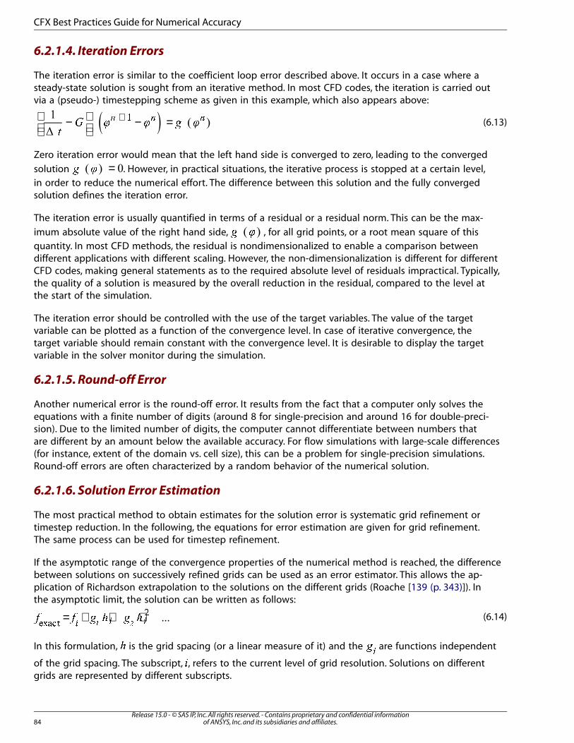
6.2.1.4. Iteration Errors
The iteration error is similar to the coefficient loop error described above. It occurs in a case where asteady-state solution is sought from an iterative method. In most CFD codes, the iteration is carried outvia a (pseudo-) timestepping scheme as given in this example, which also appears above:
(6.13)
−
− =+�
� � � � �� � ��
Zero iteration error would mean that the left hand side is converged to zero, leading to the converged
solution =� � . However, in practical situations, the iterative process is stopped at a certain level,in order to reduce the numerical effort. The difference between this solution and the fully convergedsolution defines the iteration error.
The iteration error is usually quantified in terms of a residual or a residual norm. This can be the max-
imum absolute value of the right hand side, � , for all grid points, or a root mean square of thisquantity. In most CFD methods, the residual is nondimensionalized to enable a comparison betweendifferent applications with different scaling. However, the non-dimensionalization is different for differentCFD codes, making general statements as to the required absolute level of residuals impractical. Typically,the quality of a solution is measured by the overall reduction in the residual, compared to the level atthe start of the simulation.
The iteration error should be controlled with the use of the target variables. The value of the targetvariable can be plotted as a function of the convergence level. In case of iterative convergence, thetarget variable should remain constant with the convergence level. It is desirable to display the targetvariable in the solver monitor during the simulation.
6.2.1.5. Round-off Error
Another numerical error is the round-off error. It results from the fact that a computer only solves theequations with a finite number of digits (around 8 for single-precision and around 16 for double-preci-sion). Due to the limited number of digits, the computer cannot differentiate between numbers thatare different by an amount below the available accuracy. For flow simulations with large-scale differences(for instance, extent of the domain vs. cell size), this can be a problem for single-precision simulations.Round-off errors are often characterized by a random behavior of the numerical solution.
6.2.1.6. Solution Error Estimation
The most practical method to obtain estimates for the solution error is systematic grid refinement ortimestep reduction. In the following, the equations for error estimation are given for grid refinement.The same process can be used for timestep refinement.
If the asymptotic range of the convergence properties of the numerical method is reached, the differencebetween solutions on successively refined grids can be used as an error estimator. This allows the ap-plication of Richardson extrapolation to the solutions on the different grids (Roache [139 (p. 343)]). Inthe asymptotic limit, the solution can be written as follows:
(6.14)= + + + � � � � �����
�
� �
In this formulation, � is the grid spacing (or a linear measure of it) and the �� are functions independent
of the grid spacing. The subscript, �, refers to the current level of grid resolution. Solutions on differentgrids are represented by different subscripts.
Release 15.0 - © SAS IP, Inc. All rights reserved. - Contains proprietary and confidential informationof ANSYS, Inc. and its subsidiaries and affiliates.84
CFX Best Practices Guide for Numerical Accuracy
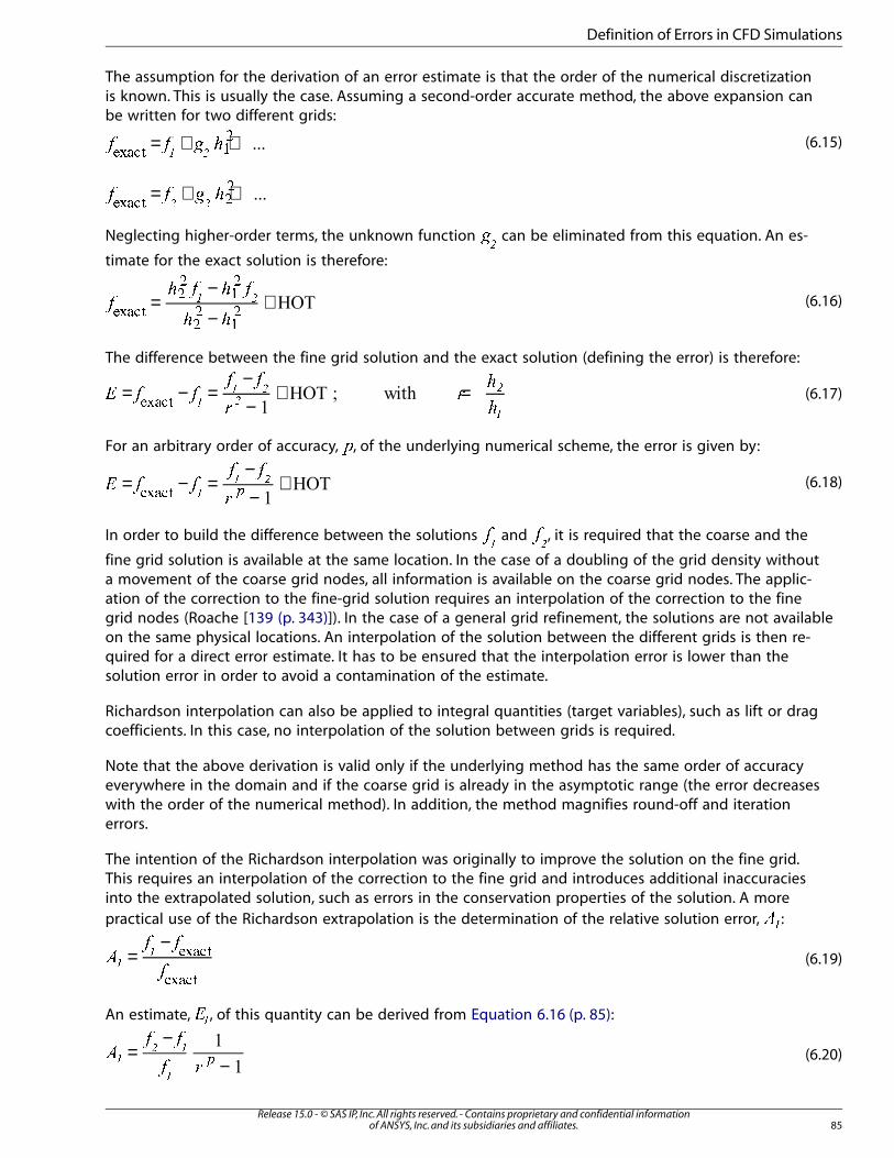
The assumption for the derivation of an error estimate is that the order of the numerical discretizationis known. This is usually the case. Assuming a second-order accurate method, the above expansion canbe written for two different grids:
(6.15)= + +� � � ������ �
�
= + +� � ������ �
�
� �
Neglecting higher-order terms, the unknown function �� can be eliminated from this equation. An es-
timate for the exact solution is therefore:
(6.16)=−
−+�
� � � �
� ������
��
�
��
�
! "
The difference between the fine grid solution and the exact solution (defining the error) is therefore:
(6.17)= − =−−
+ =# $ $$ $
%%
&
&'()*+ ,, --
-
,
For an arbitrary order of accuracy, ., of the underlying numerical scheme, the error is given by:
(6.18)= − =−−
+/ 0 00 0
1234567 88 9
In order to build the difference between the solutions :; and <
=, it is required that the coarse and the
fine grid solution is available at the same location. In the case of a doubling of the grid density withouta movement of the coarse grid nodes, all information is available on the coarse grid nodes. The applic-ation of the correction to the fine-grid solution requires an interpolation of the correction to the finegrid nodes (Roache [139 (p. 343)]). In the case of a general grid refinement, the solutions are not availableon the same physical locations. An interpolation of the solution between the different grids is then re-quired for a direct error estimate. It has to be ensured that the interpolation error is lower than thesolution error in order to avoid a contamination of the estimate.
Richardson interpolation can also be applied to integral quantities (target variables), such as lift or dragcoefficients. In this case, no interpolation of the solution between grids is required.
Note that the above derivation is valid only if the underlying method has the same order of accuracyeverywhere in the domain and if the coarse grid is already in the asymptotic range (the error decreaseswith the order of the numerical method). In addition, the method magnifies round-off and iterationerrors.
The intention of the Richardson interpolation was originally to improve the solution on the fine grid.This requires an interpolation of the correction to the fine grid and introduces additional inaccuraciesinto the extrapolated solution, such as errors in the conservation properties of the solution. A morepractical use of the Richardson extrapolation is the determination of the relative solution error, >?:
(6.19)=−
@A A
A
BCDEF
BCDEF
GG
An estimate, HI, of this quantity can be derived from Equation 6.16 (p. 85):
(6.20)=−
−J
K K
K LMN
O N
N
85Release 15.0 - © SAS IP, Inc. All rights reserved. - Contains proprietary and confidential information
of ANSYS, Inc. and its subsidiaries and affiliates.
Definition of Errors in CFD Simulations
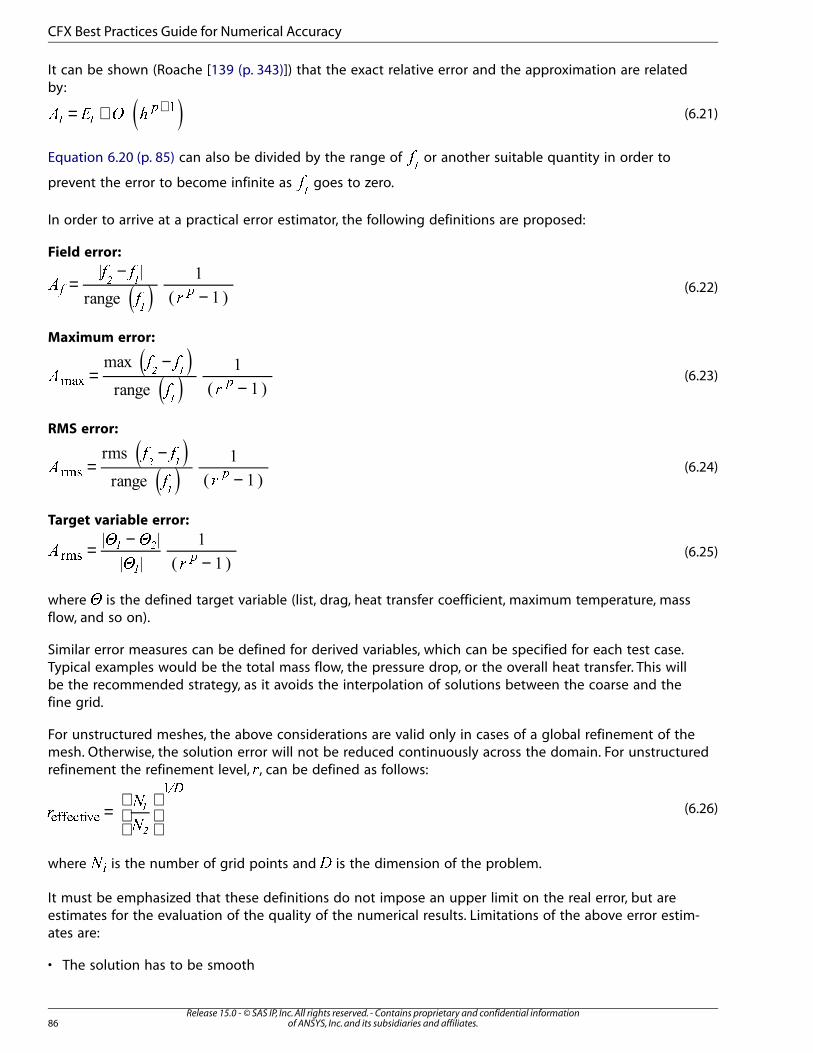
It can be shown (Roache [139 (p. 343)]) that the exact relative error and the approximation are relatedby:
(6.21)= + +� � � �
� �� �
Equation 6.20 (p. 85) can also be divided by the range of �� or another suitable quantity in order to
prevent the error to become infinite as goes to zero.
In order to arrive at a practical error estimator, the following definitions are proposed:
Field error:
(6.22)=−
−�
� �
� � �
� �
�
Maximum error:
(6.23)=−
−�
� �
� �����
� �
�
RMS error:
(6.24)=−
−�
� �
� ��� !
" #
#
Target variable error:
(6.25)= −−
$% %
% &'()*
+ ,
+
where - is the defined target variable (list, drag, heat transfer coefficient, maximum temperature, massflow, and so on).
Similar error measures can be defined for derived variables, which can be specified for each test case.Typical examples would be the total mass flow, the pressure drop, or the overall heat transfer. This willbe the recommended strategy, as it avoids the interpolation of solutions between the coarse and thefine grid.
For unstructured meshes, the above considerations are valid only in cases of a global refinement of themesh. Otherwise, the solution error will not be reduced continuously across the domain. For unstructuredrefinement the refinement level, ., can be defined as follows:
(6.26)=
/
0
0
1
233245672
89
:
;
where <= is the number of grid points and > is the dimension of the problem.
It must be emphasized that these definitions do not impose an upper limit on the real error, but areestimates for the evaluation of the quality of the numerical results. Limitations of the above error estim-ates are:
• The solution has to be smooth
Release 15.0 - © SAS IP, Inc. All rights reserved. - Contains proprietary and confidential informationof ANSYS, Inc. and its subsidiaries and affiliates.86
CFX Best Practices Guide for Numerical Accuracy

• The truncation error order of the method has to be known
• The solution has to be sufficiently converged in the iteration domain
• The coarse grid solution has to be in the asymptotic range.
For three-dimensional simulations, the demand that the coarse grid solution be in the asymptotic rangeis often hard to ensure. It is therefore required to compute the error for three different grid levels, toavoid fortuitous results. If the solution is in the asymptotic range, the following indicator should beclose to constant:
(6.27)=��
� �
6.2.2. Modeling Errors
In industrial CFD methods, numerous physical and chemical models are incorporated. Models are usuallyapplied to avoid the resolution of a large range of scales, which would result in excessive computingrequirements.
The classical model used in almost all industrial CFD applications is a turbulence model. It is based ontime or ensemble averaging of the equations resulting in the so-called Reynolds Averaged Navier-Stokes
(RANS) equations. Due to the averaging procedure, information from the full Navier-Stokes equationsis lost. It is supplied back into the code by the turbulence model. The most widely used industrial
models are two-equation models, such as the − � or −� models.
The statistical model approach reduces the resolution requirements in time and space by many ordersof magnitude, but requires the calibration of model coefficients for certain classes of flows against ex-perimental data. There is a wide variety of models that are introduced to reduce the resolution require-ments for CFD simulations, including:
• Turbulence models
• Multi-phase models
• Combustion models
• Radiation models.
In combustion models, the reduction can be both in terms of the chemical species and in terms of theturbulence-combustion interaction. In radiation, the reduction is typically in terms of the wavelengthand/or the directional information. For multi-phase flows, it is usually not possible to resolve a largenumber of individual bubbles or droplets. In this case, the equations are averaged over the differentphases to produce continuous distributions for each phase in space and time.
As all of these models are based on a reduction of the ‘real’ physics to a reduced ‘resolution’, informationhas to be introduced from outside the original equations. This is usually achieved by experimental cal-ibration, or by available DNS (p. 80) results.
Once a model has been selected, the accuracy of the simulation cannot be increased beyond the cap-abilities of the model. This is the largest factor of uncertainty in CFD methods, as modeling errors canbe of the order of 100% or more. These large errors occur in cases where the CFD solution is verysensitive to the model assumptions and where a model is applied outside its range of calibration.
87Release 15.0 - © SAS IP, Inc. All rights reserved. - Contains proprietary and confidential information
of ANSYS, Inc. and its subsidiaries and affiliates.
Definition of Errors in CFD Simulations
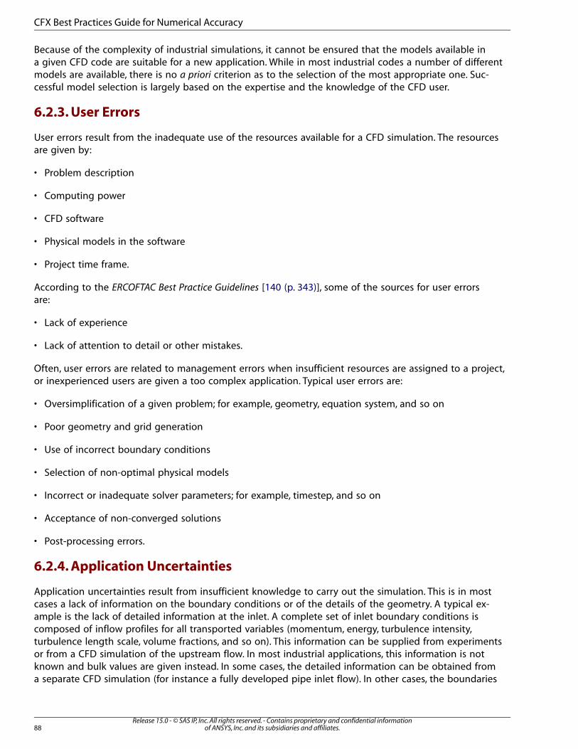
Because of the complexity of industrial simulations, it cannot be ensured that the models available ina given CFD code are suitable for a new application. While in most industrial codes a number of differentmodels are available, there is no a priori criterion as to the selection of the most appropriate one. Suc-cessful model selection is largely based on the expertise and the knowledge of the CFD user.
6.2.3. User Errors
User errors result from the inadequate use of the resources available for a CFD simulation. The resourcesare given by:
• Problem description
• Computing power
• CFD software
• Physical models in the software
• Project time frame.
According to the ERCOFTAC Best Practice Guidelines [140 (p. 343)], some of the sources for user errorsare:
• Lack of experience
• Lack of attention to detail or other mistakes.
Often, user errors are related to management errors when insufficient resources are assigned to a project,or inexperienced users are given a too complex application. Typical user errors are:
• Oversimplification of a given problem; for example, geometry, equation system, and so on
• Poor geometry and grid generation
• Use of incorrect boundary conditions
• Selection of non-optimal physical models
• Incorrect or inadequate solver parameters; for example, timestep, and so on
• Acceptance of non-converged solutions
• Post-processing errors.
6.2.4. Application Uncertainties
Application uncertainties result from insufficient knowledge to carry out the simulation. This is in mostcases a lack of information on the boundary conditions or of the details of the geometry. A typical ex-ample is the lack of detailed information at the inlet. A complete set of inlet boundary conditions iscomposed of inflow profiles for all transported variables (momentum, energy, turbulence intensity,turbulence length scale, volume fractions, and so on). This information can be supplied from experimentsor from a CFD simulation of the upstream flow. In most industrial applications, this information is notknown and bulk values are given instead. In some cases, the detailed information can be obtained froma separate CFD simulation (for instance a fully developed pipe inlet flow). In other cases, the boundaries
Release 15.0 - © SAS IP, Inc. All rights reserved. - Contains proprietary and confidential informationof ANSYS, Inc. and its subsidiaries and affiliates.88
CFX Best Practices Guide for Numerical Accuracy
can be moved far enough away from the area of interest to minimize the influence of the required as-sumptions for the complete specification of the boundary conditions.
Typical application uncertainties are:
• Lack of boundary condition information
• Insufficient information on the geometry
• Uncertainty in experimental data for solution evaluation.
6.2.5. Software Errors
Software errors are defined as any inconsistency in the software package. This includes the code, itsdocumentation, and the technical service support. Software errors occur when the information youhave on the equations to be solved by the software is different from the actual equations solved bythe code. This difference can be a result of:
• Coding errors (bugs)
• Errors in the graphical user interface (GUI)
• Documentation errors
• Incorrect support information.
6.3. General Best Practice Guidelines
In order to reduce the numerical errors, it is necessary to have procedures for the estimation of thedifferent errors described in Definition of Errors in CFD Simulations (p. 80). The main goal is to reducethe solution error to a minimum with given computer resources.
6.3.1. Avoiding User Errors
User errors are directly related to the expertise, the thoroughness, and the experience of the user. Fora given user, these errors can only be minimized by good project management and thorough interactionwith others. In case of inexperienced users, day-to-day interaction with a CFD expert/manager is requiredto avoid major quality problems. A structured work plan with intermediate results is important for inter-mediate and long-term projects.
A careful study of the CFD code documentation and other literature on the numerical methods as wellas the physical models is highly recommended. Furthermore, benchmark studies are recommended toenable you to understand the capabilities and limitations of CFD methods. A comparison of differentCFD methods is desirable, but not always possible.
6.3.2. Geometry Generation
Before the grid generation can start, the geometry has to be created or imported from CAD-data. Inboth cases, attention should be given to:
• The use of a correct coordinate system
• The use of the correct units
89Release 15.0 - © SAS IP, Inc. All rights reserved. - Contains proprietary and confidential information
of ANSYS, Inc. and its subsidiaries and affiliates.
General Best Practice Guidelines

• The use of geometrical simplification, for example, symmetry planes
• Local details. In general, geometrical features with dimensions below the local mesh size (for example,wall roughness or porous elements) are not included in the geometrical model. These should be incorpor-ated through a suitable model.
In the case that the geometry is imported from CAD-data, the data should be checked beforehand.Frequently, after the import of CAD-data, the CAD-data has to be adapted (cleaned) before it can beused for mesh generation. It is essential for mesh generation to have closed volumes. The various CAD-data formats do not always contain these closed volumes. Therefore, the CAD-data has to be alteredin order to create the closed volumes. It has to be ensured that these changes do not influence theflow to be computed.
6.3.3. Grid Generation
In a CFD analysis, the flow domain is subdivided in a large number of computational cells. All thesecomputational cells together form the so-called mesh or grid. The number of cells in the mesh shouldbe taken sufficiently large, such that an adequate resolution is obtained for the representation of thegeometry of the flow domain and the expected flow phenomena in this domain.
A good mesh quality is essential for performing a good CFD analysis. Therefore, assessment of the meshquality before performing a large and complex CFD analysis is very important. Most of the mesh gener-ators and CFD solvers offer the possibility of checking the mesh on several cells or mesh parameters,such as aspect ratio, internal angle, face warpage, right handiness, negative volumes, cracks, and tetra-hedral quality. The reader is referred to the user's guides of the various mesh generators and CFDsolvers for more information on these cells and mesh parameters.
Recommendations for grid generation are:
• Avoid high grid stretching ratios.
– Aspect ratios should not be larger than 20 to 50 in regions away from the boundary.
– Aspect ratios may be larger than that in unimportant regions.
– Aspect ratios may, and should, be larger than that in the boundary layers. For well resolved boundary
layers at high Re numbers, the near-wall aspect ratios can be of the order of 105-106.
• Avoid jumps in grid density.
– Growth factors should be smaller than 1.3.
• Avoid poor grid angles.
• Avoid non-scalable grid topologies. Non-scalable topologies can occur in block-structured grids and arecharacterized by a deterioration of grid quality under grid refinement.
• Avoid non-orthogonal, for example, unstructured tetrahedral meshes, in (thin) boundary layers.
• Use a finer and more regular grid in critical regions, for example, regions with high gradients or largechanges such as shocks.
• Avoid the presence of arbitrary grid interfaces, mesh refinements, or changes in element types in criticalregions. An arbitrary grid interface occurs when there is no one-to-one correspondence between the cellfaces on both sides of a common interface, between adjacent mesh parts.
Release 15.0 - © SAS IP, Inc. All rights reserved. - Contains proprietary and confidential informationof ANSYS, Inc. and its subsidiaries and affiliates.90
CFX Best Practices Guide for Numerical Accuracy
If possible, determine the size of the cells adjacent to wall boundaries where turbulence models areused, before grid generation has started.
Numerical diffusion is high when computational cells are created that are not orthogonal to the fluidflow. If possible, avoid computational cells that are not orthogonal to the fluid flow.
Judge the mesh quality by using the possibilities offered by the mesh generator. Most mesh generatorsoffer checks on mesh parameters, such as aspect ratio, internal angle, face warpage, right handiness,negative volumes, cracks, and tetrahedral quality.
It should be demonstrated that the final result of the calculations is independent of the grid that isused. This is usually done by comparison of the results of calculations on grids with different grid sizes.
Some CFD methods enable the application of grid adaptation procedures. In these methods, the gridis refined in critical regions (high truncation errors, large solution gradients, and so on). In these methods,the selection of appropriate indicator functions for the adaptation is essential for the success of thesimulations. They should be based on the most important flow features to be computed.
As a general rule, any important shear layer in the flow (boundary layer, mixing layer, free jets, wakes,and so on) should be resolved with at least 10 nodes normal to the layer. This is a very challenging re-quirement that often requires the use of grids that are aligned with the shear layers.
6.3.4. Model Selection and Application
Modeling errors are the most difficult errors to avoid, as they cannot be reduced systematically. Themost important factor for the reduction of modeling errors is the quality of the models available in theCFD package and the experience of the user. There is also a strong interaction between modeling errorsand the time and space resolution of the grid. The resolution has to be sufficient for the model selectedfor the application.
In principle, modeling errors can only be estimated in cases where the validation of the model is ‘close’to the intended application. Model validation is essential for the level of confidence you can have in aCFD simulation. It is therefore required that you gather all available information on the validation ofthe selected model, both from the open literature and from the code developers (vendors). In case thatCFD is to be applied to a new field, it is recommended that you carry out additional validation studies,in order to gain confidence that the physical models are adequate for the intended simulation.
If several modeling options are available in the code (as is usually the case for turbulence, combustionand multi-phase flow models), it is recommended that you carry out the simulation with differentmodels in order to test the sensitivity of the application with respect to the model selection.
In case you have personal access to a modeling expert in the required area, it is recommended thatyou interact with the model developer or expert to ensure the optimal selection and use of the model.
6.3.4.1. Turbulence Models
There are different methods for the treatment of turbulent flows. The need for a model results fromthe inability of CFD simulations to fully resolve all time and length scales of a turbulent motion. Inclassical CFD methods, the Navier-Stokes equations are usually time- or ensemble-averaged, reducingthe resolution requirements by many orders of magnitude. The resulting equations are the RANS (p. 87)equations. Due to the averaging procedure, information is lost, which is then fed back into the equationsby a turbulence model.
91Release 15.0 - © SAS IP, Inc. All rights reserved. - Contains proprietary and confidential information
of ANSYS, Inc. and its subsidiaries and affiliates.
General Best Practice Guidelines

The amount of information that has to be provided by the turbulence model can be reduced if thelarge time and length scales of the turbulent motion are resolved. The equations for this so-called Large
Eddy Simulation (LES) method are usually filtered over the grid size of the computational cells. All scalessmaller than the resolution of the mesh are modeled and all scales larger than the cells are computed.This approach is several orders of magnitude more expensive than a RANS (p. 87) simulation and istherefore not used routinely in industrial flow simulations. It is most appropriate for free shear flows,as the length scales near the solid walls are usually very small and require small cells even for theLES (p. 92) method.
RANS (p. 87) methods are the most widely used approach for CFD simulations of industrial flows. Earlymethods, using algebraic formulations, have been largely replaced by more general transport equationmodels, for both implementation and accuracy considerations. The use of algebraic models is not re-commended for general flow simulations, due to their limitations in generality and their geometric re-strictions. The lowest level of turbulence models that offer sufficient generality and flexibility are two-equation models. They are based on the description of the dominant length and time scale by two in-dependent variables. Models that are more complex have been developed and offer more generalplatforms for the inclusion of physical effects. The most complex RANS (p. 87) model used in industrialCFD applications are Second Moment Closure (SMC) models. Instead of two equations for the two mainturbulent scales, this approach requires the solution of seven transport equations for the independentReynolds stresses and one length (or related) scale.
The challenge for the user of a CFD method is to select the optimal model for the application at handfrom the models available in the CFD method. In most cases, it cannot be specified beforehand whichmodel will offer the highest accuracy. However, there are indications as to the range of applicability ofdifferent turbulence closures. This information can be obtained from validation studies carried out withthe model.
In addition to the accuracy of the model, consideration has to be given to its numerical properties andthe required computer power. It is often observed that more complex models are less robust and requiremany times more computing power than the additional number of equations would indicate. Frequently,the complex models cannot be converged at all, or, in the worst case, the code becomes unstable andthe solution is lost.
It is not trivial to provide general rules and recommendations for the selection and use of turbulencemodels for complex applications. Different CFD groups have given preference to different models forhistorical reasons or personal experiences. Even turbulence experts cannot always agree as to whichmodel offers the best cost-performance ratio for a new application.
6.3.4.1.1. One-equation Models
A number of one-equation turbulence models based on an equation for the eddy viscosity have beendeveloped over the last years. Typical applications are:
• Airplane- and wing flows
• External automobile aerodynamics
• Flow around ships.
These models have typically been optimized for aerodynamic flows and are not recommended as gen-eral-purpose models.
Release 15.0 - © SAS IP, Inc. All rights reserved. - Contains proprietary and confidential informationof ANSYS, Inc. and its subsidiaries and affiliates.92
CFX Best Practices Guide for Numerical Accuracy
6.3.4.1.2. Two-equation Models
The two-equation models are the main-stand of industrial CFD simulations. They offer a good compromisebetween complexity, accuracy and robustness. The most popular models are the standard model and
different versions of the −� model, see Wilcox [30 (p. 327)]. The standard −� model of Wilcox is the
most well known of the −� based models, but shows a severe free-stream dependency. It is thereforenot recommended for general industrial flow simulations, as the results are strongly dependent on theuser input. Alternative formulations are available, see for example, the Shear Stress Transport (SST)model, Menter [9 (p. 324)].
An important weakness of standard two-equation models is that they are insensitive to streamlinecurvature and system rotation. Particularly for swirling flows, this can lead to an over-prediction of tur-bulent mixing and to a strong decay of the core vortex. There are curvature correction models available,but they have not been generally validated for complex flows.
The standard two-equation models can also exhibit a strong build-up of turbulence in stagnation regions,due to their modeling of the production terms. Several modifications are available to reduce this effect,for instance by Kato and Launder [128 (p. 341)]. They should be used for flows around rods, blades, airfoils,and so on.
6.3.4.1.3. Second Moment Closure (SMC) Models
SMC (p. 92) models are based on the solution of a transport equation for each of the independentReynolds stresses in combination with the �- or the �-equation. These models offer generally a widermodeling platform and account for certain effects due to their exact form of the turbulent productionterms. Some of these models show the proper sensitivity to swirl and system rotation, which have tobe modeled explicitly in a two-equation framework. SMC (p. 92) models are also superior for flows instagnation regions, where no additional modifications are required.
One of the weak points of the SMC (p. 92) closure is that the same scale equations are used as in thetwo-equation framework. As the scale equation is typically one of the main sources of uncertainty, it isfound that SMC (p. 92) models do not consistently produce superior results compared to the simplermodels. In addition, experience has shown that SMC (p. 92) models are often much harder to handlenumerically. The model can introduce a strong nonlinearity into the CFD method, leading to numericalproblems in many applications.
SMC (p. 92) models are usually not started from a pre-specified initial condition, but from an alreadyavailable solution from a two-equation (or simpler) model. This reduces some of the numerical problemsof the SMC (p. 92) approach. In addition, it offers an important sensitivity study, as it allows quantifyingthe influence of the turbulence model on the solution. It is therefore recommended that you fullyconverge the two-equation model solution and save it for a comparison with the SMC (p. 92) modelsolution. The difference between the solutions is a measure of the influence of the turbulence modeland therefore an indication of the modeling uncertainty. This is possible only in steady-state simulations.For unsteady flows, the models usually have to be started from the initial condition.
6.3.4.1.4. Large Eddy Simulation Models
LES (p. 92) models are based on the numerical resolution of the large turbulence scales and the mod-eling of the small scales. LES (p. 92) is not yet a widely used industrial approach, due to the large costof the required unsteady simulations. For certain classes of applications, LES (p. 92) will be applicablein the near future. The most appropriate area will be free shear flows, where the large scales are of theorder of the solution domain (or only an order of magnitude smaller). For boundary layer flows, theresolution requirements are much higher, as the near-wall turbulent length scales become much smaller.
93Release 15.0 - © SAS IP, Inc. All rights reserved. - Contains proprietary and confidential information
of ANSYS, Inc. and its subsidiaries and affiliates.
General Best Practice Guidelines
The internal flows (pipe flows, channel flows) are in between, as they have a restricted domain in thewall normal direction, but small scales have to be resolved in the other two directions.
LES (p. 92) simulations do not easily lend themselves to the application of grid refinement studies bothin the time and the space domain. The main reason is that the turbulence model adjusts itself to theresolution of the grid. Two simulations on different grids are therefore not comparable by asymptoticexpansion, as they are based on different levels of the eddy viscosity and therefore on a different resol-ution of the turbulent scales. From a theoretical standpoint, the problem can be avoided, if the LES (p. 92)model is not based on the grid spacing, but on a pre-specified filter-width. This would enable reachinggrid-independent LES (p. 92) solutions above the DNS (p. 80) limit. However, LES (p. 92) is a very ex-pensive method and systematic grid and timestep studies are prohibitive even for a pre-specified filter.It is one of the disturbing facts that LES (p. 92) does not lend itself naturally to quality assurance usingclassical methods. This property of the LES (p. 92) also indicates that (nonlinear) multigrid methods ofconvergence acceleration are not suitable in this application.
On a more global level, the grid convergence can be tested using averaged quantities resulting fromthe LES (p. 92) simulation. The averaged LES (p. 92) results can be analyzed in a similar way asRANS (p. 87) solutions (at least qualitatively). Again, it is expensive to perform several LES (p. 92) simu-lations and grid refinement will therefore be more the exception than the rule.
Due to the high computing requirements of LES (p. 92), modern developments in the turbulencemodels focus on a combination of RANS (p. 87) and LES (p. 92) models. The goal is to cover the wallboundary layers with RANS (p. 87) and to enable unsteady (LES (p. 92)-like) solutions in largely separatedand unsteady flow regions (for example, flow behind a building, or other blunt bodies). There are twoalternatives of such methods available in ANSYS CFX.
The first alternative is called Scale-Adaptive-Simulation (SAS) model (Menter and Egorov [130 (p. 342)],[131 (p. 342)], [144 (p. 344)], [145 (p. 344)]). It is essentially an improved Unsteady RANS (URANS) methodthat develops LES (p. 92)-like solutions in unstable flow regimes.
The second alternative is called Detached Eddy Simulation (DES) (Spalart [146 (p. 344)]), implemented inthe version of Strelets [58 (p. 331)]. The current recommendation is to use the SAS (p. 94) model, as ithas less grid sensitivity than the DES (p. 94) formulation. In case that SAS (p. 94) does not provide anunsteady solution, the DES (p. 94) model should be applied. It should be noted that both model formu-lations require small timesteps with a Courant number of CFL<1. You are encouraged to read the ori-ginal references before applying these models.
6.3.4.1.5. Wall Boundary Conditions
There are generally three types of boundary conditions that can be applied to a RANS (p. 87) simulation:
• Wall Function Boundary Conditions (p. 94)
• Integration to the wall (low-Reynolds number formulation) (p. 95)
• Mixed formulation (automatic near-wall treatment) (p. 95).
6.3.4.1.5.1. Wall Function Boundary Conditions
Standard wall functions are based on the assumption that the first grid point off the wall (or the firstintegration point) is located in the universal law-of-the-wall or logarithmic region. Wall functions elim-inate the need to resolve the very thin viscous sublayer, leading to a reduction in the number of cellsand to a more moderate (and desirable) aspect ratio of the cells (ratio of the longest to the smallestside in a structured grid). High aspect ratios can result in numerical problems due to round-off errors.
Release 15.0 - © SAS IP, Inc. All rights reserved. - Contains proprietary and confidential informationof ANSYS, Inc. and its subsidiaries and affiliates.94
CFX Best Practices Guide for Numerical Accuracy
On the other hand, standard wall function formulations are difficult to handle, because you have toensure that the grid resolution near the wall satisfies the wall function requirements. If the grid becomestoo coarse, the resolution of the boundary layer is no longer ensured. If the resolution becomes toofine, the first grid spacing can be too small to bridge the viscous sublayer. In this case, the logarithmicprofile assumptions are no longer satisfied. You have to ensure that both limits are not overstepped inthe grid generation phase.
The lower limit on the grid resolution for standard wall functions is a severe detriment to a systematicgrid refinement process, as required by the best practice approach. In other words, instead of an improvedaccuracy of the solution with grid refinement, the solution will deteriorate from a certain level on,leading eventually to a singularity of the numerical method. Standard wall functions are therefore notrecommended for systematic grid refinement studies. Recently, alternative formulations (scalable wallfunctions) have become available, Menter and Esch [142 (p. 343)], which enable a systematic grid refine-ment when using wall functions.
6.3.4.1.5.2. Integration to the wall (low-Reynolds number formulation)
The use of low-Reynolds (low-Re) number formulations of turbulence models for the integration of theequations through the viscous sublayer is generally more accurate, as no additional assumptions arerequired concerning the variation of the variables near the wall. On the downside, most low-Re extensionsof turbulence models are quite complex and can reduce the numerical performance or even destabilizethe numerical method. In addition, classical low-Re models require a very fine near-wall resolution of
∼+� at all wall nodes. This is very hard to ensure for all walls of a complex industrial application. Inthe case that significantly coarser grids are used, the wall shear stress and the wall heat transfer can bereduced significantly below their correct values.
6.3.4.1.5.3. Mixed formulation (automatic near-wall treatment)
In ANSYS CFX, hybrid methods are available for all �-equation based turbulence models (automaticnear-wall treatment), which automatically switch from a low-Re formulation to wall functions based onthe grid spacing you provide. These formulations provide the optimal boundary condition for a givengrid. From a best practice standpoint, they are the most desirable, as they enable an accurate near-walltreatment over a wide range of grid spacings. However, accurate boundary layer simulations do not
depend only on the +� near-wall spacing, but also require a minimum of at least 10 grid nodes inside
the boundary layer.
6.3.4.1.5.4. Recommendations for Model Selection
• Avoid the use of classical wall functions, as they are inconsistent with grid refinement.
• Avoid strict low-Re number formulations, unless it is ensured that all near-wall cells are within the resolutionrequirements of the formulation.
• In combination with the − � model, use scalable wall functions. They can be applied to a range of gridswithout immediate deterioration of the solution (default in ANSYS CFX).
• For more accurate simulations, use an automatic wall treatment in combination with SST (p. 93) turbulencemodel (default in ANSYS CFX).
6.3.4.2. Heat Transfer Models
The heat transfer formulation is strongly linked to the underlying turbulence model. For eddy viscositymodels, the heat transfer simulation is generally based on the analogy between heat and momentum
95Release 15.0 - © SAS IP, Inc. All rights reserved. - Contains proprietary and confidential information
of ANSYS, Inc. and its subsidiaries and affiliates.
General Best Practice Guidelines
transfer. Given the eddy viscosity of the two-equation model, the heat transfer prediction is based onthe introduction of a molecular and a turbulent Prandtl number. The treatment of the energy equationis therefore similar to the treatment of the momentum equations. No additional transport equationsare required for the turbulent heat transfer prediction. The boundary conditions are the same as forthe momentum equations and follow the same recommendations.
For SMC (p. 92) models, three additional transport equations must be solved for the turbulent heattransfer vector in order to be consistent with the overall closure level. Only a few CFD methods offerthis option. In most cases, the heat transfer is computed from an eddy diffusivity with a constant turbulentPrandtl number.
6.3.4.3. Multi-Phase Models
Multi-phase models are required in cases where more than one phase is involved in the simulation(phases can also be non-miscible fluids). There is a wide variety of multi-phase flow scenarios, with thetwo extremes of small-scale mixing of the phases or a total separation of the phases by a sharp interface.
Depending on the flow simulation, different types of models are available. The main distinction of themodels is given below.
Lagrange models solve a separate equation for individual particles, bubbles, or droplets in a surroundingfluid. The method integrates the three-dimensional trajectories of the particles based on the forcesacting on them from the surrounding fluid and other sources. Turbulence is usually accounted for bya random motion, superimposed on the trajectory.
Lagrange models are usually applied to flows with low particle (bubble) densities. In these flows, theinteraction between the particles can usually be neglected, thereby reducing the complexity of theproblem significantly.
The Euler-Euler formulation is based on the assumption of interpenetrating continua. A separate set ofmass, momentum, and energy conservation equations is solved for each phase. Interphase transferterms have to be modeled to account for the interaction of the phases. Euler-Euler methods can beapplied to separated and dispersed flows by changing the interface transfer model.
Additional models are required for flows with mass transfer between the phases (condensation, evap-oration, boiling). These models can be applied in the form of correlations for a large number of particles(bubbles) in a given control volume, or directly at the interface between the resolved phase boundary.
6.3.5. Reduction of Application Uncertainties
Application uncertainties cannot always be avoided because the missing information can frequentlynot be recovered. The uncertainty can be minimized by interaction with the supplier of the test case.The potential uncertainties have to be documented before the start of the CFD application.
In the case that the assumptions have to be made concerning any input to a CFD analysis, they haveto be communicated to the partners in the project. Alternative assumptions have to be proposed andthe sensitivity of the solution to these assumptions has to be evaluated by case studies (alteration ofinflow profiles, different locations for arbitrary boundary conditions, and so on).
Recommendations are:
• Identify all uncertainties in the numerical setup:
– Geometry reduction
Release 15.0 - © SAS IP, Inc. All rights reserved. - Contains proprietary and confidential informationof ANSYS, Inc. and its subsidiaries and affiliates.96
CFX Best Practices Guide for Numerical Accuracy
– Boundary condition assumptions
– Arbitrary modeling assumptions, for example, bubble diameter, and so on.
• Perform a sensitivity analysis with at least two settings for each arbitrary parameter.
• Document the sensitivity of the solution on the assumptions.
6.3.6. CFD Simulation
This section provides recommendations concerning the optimal application of a CFD method, once thegrids are available and the basic physical models have been defined.
6.3.6.1. Target Variables
In order to monitor numerical errors, it is recommended that you define target variables. The convergenceof the numerical scheme can then be checked more easily and without interpolation between differentgrids. You should select target variables that:
1. Are representative of the goals of the simulation.
2. Are sensitive to numerical treatment and resolution.
This criteria should help to avoid the use of measures that are insensitive to the resolution, suchas pressure-based variables in boundary layer simulations.
3. Can be computed with existing post-processing tools.
4. Can be computed inside the solver and displayed during run-time (optimal).
It is optimal if the variable can be computed during run-time and displayed as part of the convergencehistory. This enables you to follow the development of the target variable during the iterative process.
6.3.6.2. Minimizing Iteration Errors
A first indication of the convergence of the solution to steady state is the reduction in the residuals.Experience shows, however, that different types of flows require different levels of residual reduction.For example, it is found regularly that swirling flows can exhibit significant changes even if the residualsare reduced by more than 5 - 6 orders of magnitude. Other flows are well converged with a reductionof only 3 - 4 orders.
In addition to the residual reduction, it is therefore required to monitor the solution during convergenceand to plot the pre-defined target quantities of the simulation as a function of the residual (or the iter-ation number). A visual observation of the solution at different levels of convergence is recommended.
It is also recommended that you monitor the global balances of conserved variables, such as mass,momentum and energy, vs. the iteration number.
Convergence is therefore monitored and ensured by the following steps:
• Reduce residuals by a pre-specified level and provide residual plots.
• Plot evolution of r.m.s. and maximum residual with iteration number.
• Report global mass balance with iteration number.
97Release 15.0 - © SAS IP, Inc. All rights reserved. - Contains proprietary and confidential information
of ANSYS, Inc. and its subsidiaries and affiliates.
General Best Practice Guidelines
• Plot target variables as a function of iteration number or residual level.
• Report target variables as a function of r.m.s. residual (table).
It is desirable to have the target variable written out at every timestep in order to display it during thesimulation run.
Depending on the numerical scheme, the recommendations may also be relevant to the iterative con-vergence within the timestep loop for transient simulations.
6.3.6.3. Minimizing Spatial Discretization Errors
Spatial discretization errors result from the numerical order of accuracy of the discretization schemeand from the grid spacing. It is well known that only second- and higher-order space discretizationmethods are able to produce high quality solutions on realistic grids. First-order methods shouldtherefore be avoided for high quality CFD simulations.
As the order of the scheme is usually given (mostly second-order), spatial discretization errors can beinfluenced only by the provision of an optimal grid. It is important for the quality of the solution andthe applicability of the error estimation procedures defined in Solution Error Estimation (p. 84), thatthe coarse grid already resolves the main features of the flow. This requires that the grid points areconcentrated in areas of large solution variation. For the reduction of spatial discretization errors, it isalso important to provide a high-quality numerical grid.
For grid convergence tests, the simulations are carried out for a minimum of three grids. The targetquantities will be given as a function of the grid density. In addition, an error estimate based on thedefinition given in Solution Error Estimation (p. 84) (Equation 6.25 (p. 86)) will be carried out. It is alsorecommended that you compute the quantity given by Equation 6.27 (p. 87) to test the assumption ofasymptotic convergence.
It is further recommended that the graphical comparison between the experiments and the simulationsshow the grid influence for some selected examples. The following information should be provided:
• Define target variable as given in Target Variables (p. 97).
• Provide three (or more) grids using the same topology (or for unstructured meshes, a uniform refinementover all cells).
• Compute solution on these grids:
– Ensure convergence of the target variable in the time- or iteration domain. See Iteration Errors (p. 84)and Minimizing Iteration Errors (p. 97).
– Compute target variables for these solutions.
• Compute and report error measure for target variable(s) based on Equation 6.25 (p. 86).
• Plot selected variables for the different grids in one picture.
• Check if the solution is in the asymptotic range using Equation 6.27 (p. 87).
6.3.6.4. Minimizing Time Discretization Errors
In order to reduce time integration errors for unsteady-state simulations, it is recommended that youuse at least a second-order-accurate time-discretization scheme. Usually, the relevant frequencies can
Release 15.0 - © SAS IP, Inc. All rights reserved. - Contains proprietary and confidential informationof ANSYS, Inc. and its subsidiaries and affiliates.98
CFX Best Practices Guide for Numerical Accuracy
be estimated beforehand and the timestep can be adjusted to provide at least 10 - 20 steps for eachperiod of the highest relevant frequency. In case of unsteadiness due to a moving front, the timestepshould be chosen as a fraction of:
(6.28)∼� �
�
with the grid spacing � and the front speed � .
It should be noted that under strong grid and timestep refinement, sometimes flow features are resolvedthat are not relevant for the simulation. An example is the (undesirable) resolution of the vortex sheddingat the trailing edge of an airfoil or a turbine blade in a RANS (p. 87) simulation for very fine grids andtimesteps. Another example is the gradual switch to a DNS (p. 80) for the simulation of free surfaceflows with a Volume of Fluid (VOF) method (for example, drop formation, wave excitation for freesurfaces, and so on). This is a difficult situation, as it usually means that no grid/timestep convergedsolution exists below the DNS (p. 80) range, which can usually not be achieved.
In principle, the time dependency of the solution can be treated as another dimension of the problemwith the definitions in Solution Error Estimation (p. 84). However, a four-dimensional grid study wouldbe very demanding. It is therefore more practical to carry out the error estimation in the time domainseparately from the space discretization. Under the assumption that a sufficiently fine space discretizationis available, the error estimation in the time domain can be performed as a one-dimensional study.
Studies should be carried out with at least two and if possible three different timesteps for one givenspatial resolution. Again, the error estimators given in Solution Error Estimation (p. 84) (Equa-tion 6.25 (p. 86)) can be used, if is replaced by the timestep. The following information should beprovided:
• Unsteady target variables as a function of timestep (graphical representation)
• Error estimate based on Equation 6.25 (p. 86) for (time averaged) target variables
• Comparison with experimental data for different timesteps.
6.3.6.5. Avoiding Round-Off Errors
Round-off errors are usually not a significant problem. They can occur for high-Reynolds number flowswhere the boundary layer resolution can lead to very small cells near the wall. The number of digits ofa single precision simulation can be insufficient for such cases. The only way to avoid round-off errorswith a given CFD code is the use of a double precision version. In case of an erratic behavior of theCFD method, the use of a double precision version is recommended.
6.3.7. Handling Software Errors
Software errors can be detected by verification studies. They are based on a systematic comparison ofCFD results with verified solutions (in the optimal case analytical solutions). It is the task of the softwaredeveloper to ensure the functionality of the software by systematic testing.
In most cases, pre-existing software will be used. It is assumed that all CFD packages have been suffi-ciently tested to ensure that no software verification studies have to be carried out in the project (exceptfor newly developed modules). In case that two CFD packages give different results for the same applic-ation, using the same physical models, the sources for these differences will have to be evaluated. Incase of code errors, they will be reported to the code developers and if possible removed.
99Release 15.0 - © SAS IP, Inc. All rights reserved. - Contains proprietary and confidential information
of ANSYS, Inc. and its subsidiaries and affiliates.
General Best Practice Guidelines
6.4. Selection and Evaluation of Experimental Data
Because of the necessity to model many of the unresolved details of technical flows, it is necessary toassess the accuracy of the CFD method with the help of experimental data. Experiments are requiredfor the following tasks and purposes:
• Verification of model implementation
• Validation and calibration of statistical models
• Demonstration of model capabilities.
There is no philosophical difference between the different types of test cases. The same test case canbe used for the different phases of model development, implementation, validation, and application,depending on the status of the model and the suitability of the data.
6.4.1. Verification Experiments
The purpose of verification tests is to ensure the correct implementation of all numerical and physicalmodels in a CFD method. The best verification data would be the analytical solutions for simple casesthat enable the testing of all relevant implementation aspects of a CFD code and the models implemen-ted. As analytical solutions are not always available, simple experimental test cases are often used instead.
6.4.1.1. Description
For CFD code verification, convergence can be tested against exact analytical solutions like:
• Convection of disturbances by a given flow
• Laminar Couette flow
• Laminar channel flow.
For the verification of newly implemented models, verification can only in limited cases be based onanalytical solutions. An example is the terminal rise velocity of a spherical bubble in a calm fluid.
In most other cases, simple experiments are used for the verification. It is recommended that youcompute the test cases given by the model developer in the original publication of the model, or othertrustworthy publications. Quite often experimental correlations can be applied, without the need forcomparison with one specific experiment. For instance for turbulence model verification, the most fre-quently used correlations are those for flat plate boundary layers.
6.4.1.2. Requirements
The only requirement for verification data is that they enable a judgement of the correct implementationof the code and/or the models. This requires information from other sources concerning the performanceof the model for the test case. Strictly speaking, it is not required that the simulations are in goodagreement with the data, but that the differences between the simulations and the data are as expected.
The test suite for model verification must be diverse enough to check all aspects of the implementation.As an example, a fully developed channel flow does not enable a test of the correct implementationof the convective terms of a transport equation. The test suite should also enable testing the correctinteraction of the new model with other existing features of the software.
Release 15.0 - © SAS IP, Inc. All rights reserved. - Contains proprietary and confidential informationof ANSYS, Inc. and its subsidiaries and affiliates.100
CFX Best Practices Guide for Numerical Accuracy

Software verification for physical models should be carried out in the same environment that the end-user has available. Testing of the new features in an expert environment might miss some of errorsources, such as the GUI (p. 89).
Verification cases should be selected before the model is implemented. They must be considered anintegral part of the model implementation.
6.4.2. Validation Experiments
The purpose of validation tests is to check the quality of a statistical model for a given flow situation.Validation tests are the only method to ensure that a new model is applicable with confidence to certaintypes of flows. The more validation tests a model passes with acceptable accuracy, the more generallyit can be applied to industrial flows. The goal of validation tests is to minimize and quantify modelingerrors. Validation cases are often called building block experiments, as they test different aspects of aCFD code and its physical models. The successful simulation of these building blocks is a prerequisitefor a complex industrial flow simulation.
6.4.2.1. Description
Examples of validation cases are flows with a high degree of information required to test the differentaspects of the model formulation. In an ideal case, a validation test case should be sufficiently completeto enable an improvement of the physical models it was designed to evaluate. Increasingly, validationdata are obtained from DNS (p. 80) studies. The main limitation here is in the low-Reynolds numberand the limited physical complexity of DNS (p. 80) data. Typically, validation cases are geometricallysimple and often based on two-dimensional or axisymmetric geometries.
6.4.2.2. Requirements
Validation cases are selected to be as close as possible to the intended application of the model. As anexample, the validation of a turbulence model for a flat plate boundary layer does not ensure the ap-
plicability of the model to flows with separation (as is known from the − � model). It is well acceptedby the CFD community and by model developers that no model (turbulence, multi-phase or other) willbe able to cover all applications with sufficient accuracy. This is the reason why there are always multiplemodels for each application. The validation cases enable the CFD user to select the most appropriatemodel for the intended type of application.
Test case selection requires that the main features of the CFD models that are to be tested be clearlyidentified. They must then be dominant in the validation case. Validation cases are often ‘single physics’cases, but it will be more and more necessary to validate CFD methods for combined effects.
The requirements for validation cases are that there should be sufficient detail to be able to computethe flow unambiguously and to evaluate the performance of the CFD method for a given target applic-ation.
Completeness of information is one of the most important requirements for a validation test case. Thisincludes all information required to run the simulation, like:
• Geometry
• Boundary conditions
• Initial conditions (for unsteady flows)
• Physical effects involved.
101Release 15.0 - © SAS IP, Inc. All rights reserved. - Contains proprietary and confidential information
of ANSYS, Inc. and its subsidiaries and affiliates.
Selection and Evaluation of Experimental Data
While the first three demands are clearly necessary to be able to set up and run the simulation, theknowledge of all physical effects taking place in the experiment is not always considered. However, itis crucial to have a clear understanding of the overall flow in order to be able to judge the quality ofa test case. Typical questions are:
• Is the flow steady-state or does it have a large-scale unsteadiness?
• Is the flow two-dimensional (axisymmetric, for example)?
• Are all the relevant physical effects known (multi-phase, transition, and so on)?
• Have any corrections been applied to the data and are they appropriate?
• Was there any measurement/wind or water tunnel interference?
Completeness of information is also essential for the comparison of the simulation results with the ex-perimental data. A validation case should have sufficient detail to identify the sources for the discrep-ancies between the simulations and the data. This is a vague statement and cannot always be ensured,but a validation experiment should provide more information than isolated point measurements. Profilesand distributions of variables at least in one space dimension should be available (possibly at differentlocations). More desirable is the availability of field data in two-dimensional measuring planes includingflow visualizations.
Completeness also relates to the non-dimensionalization of the data. Frequently the information providedis not sufficient to reconstruct the data in the form required by the validation exercise.
In case that the data provided are not sufficient, the impact of the missing information has to be assessed.Most crucial is the completeness of the data required to set up the simulation. In case of missing inform-ation, the influence of this information deficit has to be assessed. Typical examples are incomplete inletboundary conditions. While the mean flow quantities are often provided, other information requiredby the method, as profiles for turbulent length scales and volume fractions is frequently missing. Theimportance of this deficit can be estimated by experience with similar flows and by sensitivity studiesduring the validation exercise.
Next to the completeness of the data, their quality is of primary importance for a successful validationexercise. The quality of the data is mainly evaluated by error bounds provided by the experimentalists.Unfortunately, most experiments still do not provide this information. Moreover, even if error estimatesare available, they cannot exclude systematic errors by the experimentalist.
In addition to error bounds, it is therefore desirable to have an overlap of experimental data that enabletesting the consistency of the measurements. Examples are the same data from different experimentaltechniques. It is also a quality criterion when different experimental groups in different facilities havecarried out the same experiment. Consistency can also be judged from total balances, like mass, mo-mentum and energy conservation. Quality and consistency can frequently be checked if validation ex-ercises have already been carried out by other CFD groups, even if they used different models.
The availability of the data has to be considered before any CFD validation is carried out. This includesquestions of ownership. For most CFD code developers, data that cannot be shown publicly are muchless valuable than freely available experimental results.
6.4.3. Demonstration Experiments
The purpose of a demonstration exercise is to build confidence in the ability of a CFD method to simulatecomplex flows. While validation studies have shown for a number of building block experiments that
Release 15.0 - © SAS IP, Inc. All rights reserved. - Contains proprietary and confidential informationof ANSYS, Inc. and its subsidiaries and affiliates.102
CFX Best Practices Guide for Numerical Accuracy
the physical models can cover the basic aspects of the target application, the demonstration cases testthe ability of a method to predict combined effects, including geometrical complexity.
6.4.3.1. Description
For an aerodynamic study, a typical hierarchy would be:
• Verification - Flat plate
• Validation - Airfoil or wing
• Demonstration - Complete aircraft.
Similar hierarchies can be established for other industrial areas.
6.4.3.2. Requirements
Typically, the detail of the experimental data is much lower than for verification or validation cases.
Completeness of information to set up the test case is of similar importance as for validation cases andinvolves the same aspects as listed below:
• Geometry
• Boundary conditions
• Initial conditions (for unsteady flows)
• Physical effects involved.
Typically, the level of completeness of the data for demonstration cases is much lower than for validationcases. It is therefore even more essential to identify the missing information and to carry out sensitivitystudies with respect to these data.
In terms of post-processing, demonstration cases often do not provide a high degree of detail. Theyare usually not appropriate to identify specific weaknesses in the physical models or the CFD codes.Typically, only the point data or global parameters, as efficiencies, are provided.
Even though the density of data is usually lower, the quality should satisfy the same criteria as for val-idation cases. Error estimates are desirable and so are independent measurements.
Due to the limited amount of data available, the information is usually not sufficient to carry out con-sistency checks.
The requirements in terms of availability/openness are usually lower than for validation cases, as thedemonstration applies usually to a smaller audience. A demonstration case might be carried out for asingle customer or one specific industrial sector. It has to be ensured, as in all cases, that the data canbe shown to the target audience of the simulation.
103Release 15.0 - © SAS IP, Inc. All rights reserved. - Contains proprietary and confidential information
of ANSYS, Inc. and its subsidiaries and affiliates.
Selection and Evaluation of Experimental Data

Release 15.0 - © SAS IP, Inc. All rights reserved. - Contains proprietary and confidential informationof ANSYS, Inc. and its subsidiaries and affiliates.104
Chapter 7: CFX Best Practices Guide for Cavitation
This guide is part of a series that provides advice for using CFX in specific engineering application areas.It is aimed at users with moderate or little experience using CFX for applications involving cavitation.
This guide describes Liquid Pumps (p. 105).
Cavitation is the formation of vapor bubbles within a liquid where flow dynamics cause the local staticpressure to drop below the vapor pressure. The bubbles of vapor usually last a short time, collapsingwhen they encounter higher pressure. Cavitation should not be confused with boiling. When a liquidboils, thermal energy drives the local temperature to exceed the saturation temperature.
Cavitation is a concern in several application areas, including pumps, inducers, marine propellers, waterturbines, and fuel injectors. One of the major problems caused by cavitation is a loss of pressure riseacross a pump. Other problems include noise, vibration, and damage to metal components.
The next section discusses the effects of cavitation on the performance of liquid pumps.
7.1. Liquid Pumps
Water pumps must take in water and deliver it at a higher total pressure with an acceptable flow rate.Under certain conditions, cavitation may occur on the low pressure side of the pump, causing a loss ofpressure rise and/or flow rate.
Both pump performance without cavitation and the affects of cavitation on performance will be discussed.
7.1.1. Pump Performance without Cavitation
As long as the static pressure remains sufficiently high everywhere in the system, cavitation will notoccur. In this case, for a given pump RPM, the pressure rise and flow rate are directly coupled, and canbe plotted in a pump performance diagram, as shown below.
105Release 15.0 - © SAS IP, Inc. All rights reserved. - Contains proprietary and confidential information
of ANSYS, Inc. and its subsidiaries and affiliates.

Figure 7.1: Flow Rate vs Pressure Rise for a Liquid Pump
7.1.2. Pump Performance with Cavitation
If the inlet total pressure is below the critical value for a particular flow rate and RPM, cavitation willoccur causing the pressure rise to diminish. The following performance diagram shows the effect ofcavitation on pressure rise.
Figure 7.2: Cavitation Performance at Constant RPM and Flow Rate
NPSH is the Net Positive Suction Head, a quantity directly related to the inlet total pressure by the relation:
(7.1)=
−
����
� �
� �
� � �� �
Release 15.0 - © SAS IP, Inc. All rights reserved. - Contains proprietary and confidential informationof ANSYS, Inc. and its subsidiaries and affiliates.106
CFX Best Practices Guide for Cavitation
where pT,inlet is the inlet total pressure, pv is the vapor pressure, � is density, and g is the acceleration
due to gravity. As the inlet total pressure drops, so does the NPSH value, and the amount of cavitationincreases.
To generate this diagram, RPM and flow rate are fixed, and the pressure rise is measured at progressivelylower inlet total pressures. For the part of the test where the inlet total pressure is sufficiently high toprevent cavitation, the pressure rise across the pump is constant, equal to the amount predicted bythe first performance diagram. This results in a horizontal trend in the performance curve as the inlettotal pressure is dropped. Because the pressure rise remains constant, the total pressure at the outletdrops by the same amount as at the inlet. Using CFX software, a mass flow outlet boundary conditioncan be specified to fix the flow rate while the inlet total pressure is varied.
When the inlet total pressure reaches a sufficiently low value, cavitation occurs. A further reduction ininlet total pressure causes more cavitation, which almost always causes a large loss of pressure rise. Inrare cases, pressure rise can actually increase slightly with small amounts of cavitation. Even in suchcases, however, a further increase in cavitation causes a sudden loss of pressure rise. In the lab, thepressure rise will eventually become insufficient to maintain the required flow rate. Using CFX software,the solution will eventually fail to converge. Before this point, data should be collected with a sufficientresolution (sufficiently small changes in inlet pressure) to resolve the part of the performance curvewhere the pressure starts to drop. The point of cavitation is often marked by the NPSH at which thepressure rise has fallen by a few percent.
7.1.3. Procedure for Plotting Performance Curve
1. Set up a simulation with cavitation turned on and pressure levels set high enough to avoid levels ofcavitation that significantly affect pressure rise.
If you have trouble getting a converged solution, try running a simulation with cavitation turnedoff, then use the result as an initial guess for a simulation with cavitation turned on.
2. Run the solver to obtain a solution.
3. Calculate the pressure rise across the pump and the NPSH value, then plot a point in the performancediagram.
4. Lower the pressure boundary condition by about 5% to 10%.
5. Repeat starting from step 2, using the previous solution as the initial guess, until cavitation has causeda significant loss of pump head.
7.1.4. Setup
To facilitate setting up typical domain settings for the cavitation of water, you may load a single-domainmesh, then run the template .ccl file:
CFX/etc/model-templates/cavitating_water.ccl
This file should be examined in a text editor before using it so that you understand which settings itspecifies.
For the domain fluids list, specify both a liquid and a vapor for the same material. In most cases, it issufficient to use a constant-density vapor.
107Release 15.0 - © SAS IP, Inc. All rights reserved. - Contains proprietary and confidential information
of ANSYS, Inc. and its subsidiaries and affiliates.
Liquid Pumps
Under Fluid Models for the domain, it is strongly recommended that you select Homogeneous Model
under Multiphase Options. You do not need to select Free Surface Model for the purpose of simulatingcavitation.
Under Fluid Pairs for the domain, select the fluid pair from the list and, for Mass Transfer, set Option
to Cavitation . Select the Rayleigh Plesset cavitation model or a User Defined Cavitation Model.For the Rayleigh Plesset model, the Mean Diameter for cavitation bubbles represents the mean nuc-leation site diameter and must be specified. The default value of 2e-06 m is a reasonable value in mostcases. The Saturation Pressure must be defined unless the materials you have selected are the com-ponents of a homogeneous binary mixture. In the latter case, the saturation properties will already bedefined in the mixture definition, but you may still choose to override the Saturation Pressure byspecifying it on the Fluid Pairs tab.
When initializing the domain, set the volume fraction of vapor to zero and the volume fraction of liquidto unity. These settings (represented by the Automatic setting for Volume Fraction) are used bydefault in CFX.
Set up the problem with one of the following boundary condition combinations:
1. Inlet total pressure and outlet mass flow (recommended)
2. Inlet velocity profile and outlet static pressure
The inlet boundary condition should specify that the volume fraction of vapor is zero.
Turbulence models should be chosen as usual (e.g., k-epsilon or SST). For turbulence induced cavitation,consider using the DES model.
For advection scheme, use high resolution, or a specified blend factor of unity.
If editing a material, remember that the vapor pressure is on an absolute scale; it does not depend onthe specified reference pressure.
Cavitation models cannot be combined with other types of interphase mass transfer, such as thermalphase changes.
7.1.5. Convergence Tips
If performing a single solution, initially turn off cavitation, then turn on cavitation and use the first setof results as an initial guess.
If performing a series of simulations using one solution to initialize the next, solve the cases in orderof decreasing pressure (i.e., approaching cavitation).
7.1.6. Post-Processing
A contour plot of volume fraction for the vapor can show where cavitation bubbles exist.
To calculate the inlet and outlet pressures, use the function calculator.
Release 15.0 - © SAS IP, Inc. All rights reserved. - Contains proprietary and confidential informationof ANSYS, Inc. and its subsidiaries and affiliates.108
CFX Best Practices Guide for Cavitation
Chapter 8: CFX Best Practices Guide for Combustion
This guide is part of a series that provides advice for using CFX in specific engineering application areas.It is aimed at users with moderate or little experience using CFX for applications involving combustion.
This guide describes:
• Gas Turbine Combustors (p. 109)
• Combustion Modeling in HVAC Cases (p. 111)
8.1. Gas Turbine Combustors
Gas turbines are widely used in stationary and aircraft applications. The combustor receives the workingfluid in a compressed state, burns fuel to increase its temperature, and passes it to the turbine. One ofthe key design goals for the combustor is to achieve a stable combustion process. Another key designgoal is to minimize the emission of pollutants, particularly oxides of nitrogen.
8.1.1. Setup
8.1.1.1. Steady State vs. Transient
Most simulations are steady-state, particularly for stationary gas turbines that operate at a constantload.
8.1.1.2. Turbulence Model
The −� � turbulence model is used in many applications, but the SST model should be considered forflows with separated boundary layers, and the Reynolds Stress Model is the best choice for highlyswirling flows.
8.1.1.3. Reference Pressure
Because of the high inlet pressure, a reference pressure between 4 and 20 atmospheres is common,and depends upon the type of simulation you are running.
8.1.1.4. Combustion Model
The choice of combustion model depends of whether the fuel/oxidant combination is premixed. Thefollowing table outlines some of the differences.
Non-Premixed CombustionPremixed Combustion
Typically used for flight engines because it iseasier to control variable operating condi-tions.
Commonly used for recent stationary gas tur-bines in power generation.
109Release 15.0 - © SAS IP, Inc. All rights reserved. - Contains proprietary and confidential information
of ANSYS, Inc. and its subsidiaries and affiliates.

Non-Premixed CombustionPremixed Combustion
Combustion Models: EDM, FRC/EDM com-bined, Flamelet (and, for some cases, also thePremixed model).
Combustion Models: EDM with product limiterand/or extinction submodels, FRC/EDM com-bined, Partially Premixed (Turbulent Flame SpeedClosure (TFC))
Note that the EDM model usually needs adjust-ing for premixed combustion (for example, ex-tinction by temperature or by mixing/chemicaltime scales).
For the preliminary analysis of high speed turbulent flow, the Eddy Dissipation combustion model is asensible choice, but cannot simulate burning velocities or flame position.
The Laminar Flamelet model is applicable for turbulent flow with non-premixed combustion, andprovides a robust solution at a low computational expense for multi-step reactions. The Flameletmodel uses a chemistry library, meaning that only two additional transport equations are solved tocalculate multiple species. As a result, the Flamelet model is a very good choice for modeling theformation of various pollutants during the combustion process. The Flamelet model predicts incompletecombustion to some extent (CO in exhaust gas), which helps to predict reduction in temperature (unlikeEDM).
8.1.2. Reactions
During the initial analysis of a combustor, the highest values of temperature and outgoing heat fluxare likely to be of primary concern. For this purpose, a single-step Eddy Dissipation reaction can beused. Such a reaction is likely to overpredict the temperature, and will not predict emissions correctly,but can provide a conservative indicator of the expected temperature levels.
Other reaction steps might then be added to the simulation to account for the formation of combustionbyproducts. Each reaction step has its own separate time scale. As a result, convergence can becomevery difficult when a multi-step reaction contains more than about 5 steps.
8.1.3. Convergence Tips
The Equation Class Settings tab in CFX-Pre can be used to set different advection schemes and timescales for each class of equation you are solving. For multi-step Eddy Dissipation reactions, convergencecan be improved by temporarily increasing the mass fraction time scale by a factor of about 5-10.
For the Eddy Dissipation Model, multistep convergence can be aided by first running a simplified single-step simulation and using the results from the run as an initial values file for a multi-step run.
You may restart a Flamelet model from a cold solution. You should avoid restarting with the Flameletmodel from an EDM solution. You may restart an EDM case from a Flamelet model solution.
The High Resolution advection scheme is always recommended for combustion simulations because itis bounded and prevents over/undershoots. Care must be taken, however, to provide a mesh of sufficientquality to resolve most of the flow features. A very poor mesh will result in the scheme using a blendfactor close to zero (therefore not providing a solution as accurate as expected).
For simulations which include Finite Rate Chemistry, small temperature variations can result in largechanges in reaction rate. When a solution is converging, temperature values may change sufficiently
Release 15.0 - © SAS IP, Inc. All rights reserved. - Contains proprietary and confidential informationof ANSYS, Inc. and its subsidiaries and affiliates.110
CFX Best Practices Guide for Combustion
to make the solution unstable. To aid convergence, add a TEMPERATURE DAMPING CCL structurewithin a SOLVER CONTROL block, as follows:
FLOW: SOLVER CONTROL: TEMPERATURE DAMPING: Option = Temperature Damping Temperature Damping Limit = <Real number> Under Relaxation Factor = <Real number> END END END
Depending on the location of the SOLVER CONTROL block, the temperature damping may be appliedto a particular domain or phase. Set the Temperature Damping Limit to 0 so that positivedamping is always applied. The Under Relaxation Factor can be set to multiply changes intemperature by a value between 0 and 1. You should try a factor of 0.2 if you are having trouble con-verging a solution.
8.1.4. Post-Processing
Some of the most common plots to create in CFD-Post include:
• Mass Fractions: fuel, O2, products, intermediate species (CO), pollutants (NO)
• Turbulent Mixing Time Scale (Eddy Dissipation / Turbulent Kinetic Energy)
• Reaction Rates
The variable "<my reaction>.Molar Reaction Rate" is available for every "Single Step" reaction (EDM,FRC or combined model).
• Plots of the turbulent Damköhler number (the ratio of the turbulent time scale to the chemical time scale)
8.2. Combustion Modeling in HVAC Cases
This section deals with the setup of combustion cases for HVAC simulations, where it is important toaccurately model the combustion process. Such processes are known as "combusting fire" simulations,as opposed to "inert fire" simulations.
Using a combusting fire simulation is the most accurate way to model fires in all HVAC cases. It is par-ticularly important in cases when the fire is under-ventilated, or when the ventilation cannot be easilypredicted. The drawback is the additional computational expense involved in solving a full combustionmodel as part of the main solution.
8.2.1. Set Up
Most simulations are set up as transient. The choice of timestep is generally model dependent, but willusually fall into the range 0.5 s to 2 s. The Total Energy heat transfer model should be selected to fullymodel buoyancy.
Note
When modeling buoyancy, it is very important to correctly specify the buoyancy referencedensity when opening boundary conditions are used.
111Release 15.0 - © SAS IP, Inc. All rights reserved. - Contains proprietary and confidential information
of ANSYS, Inc. and its subsidiaries and affiliates.
Combustion Modeling in HVAC Cases
The RNG −� � turbulence model is a good choice for combusting flows, with either no buoyancy termsin equations or buoyancy terms in both the equations (with C3=1). The SST model is also reasonable,but may not converge well for natural convection. The SSG model is accurate, but convergence maybe very slow.
The most common fuels used are hydrocarbons such as methane, diesel and petroleum. Cellulosic ma-terials, plastics and wood are also used. The simulation will dictate the type of materials to use as afuel.
The Eddy Dissipation Model is widely used, combined with an Additional Variable for toxins. Theflamelet model is more rigorous, and is a better choice when the fire is under ventilated.
8.2.2. Convergence Tips
Convergence can be slowed if care is not taken in the setup of buoyancy and openings.
The presence of an instantaneous fuel supply is sometimes not physical, and can slow convergence. Inmany transient cases, the amount of fuel available can be controlled by using time-dependent expres-sions.
8.2.3. Post-processing
The most common parameters of interest in a combusting fire model are simulation-dependent, butwill usually include one of more of the following:
• Temperature
• Products (including carbon monoxide and other toxins)
• Visibility
• Wall Temperature
• Wall convective and radiative heat fluxes
Release 15.0 - © SAS IP, Inc. All rights reserved. - Contains proprietary and confidential informationof ANSYS, Inc. and its subsidiaries and affiliates.112
CFX Best Practices Guide for Combustion
Chapter 9: CFX Best Practices Guide for HVAC
This guide discusses best practices for setting up, solving, and post processing an HVAC simulation:9.1. HVAC Simulations9.2. Convergence Tips
This guide is part of a series that provides advice for using CFX in specific engineering application areas.
It is aimed at users with moderate or little experience using CFX for HVAC1 applications.
9.1. HVAC Simulations
HVAC studies range in scale from single components (such as a radiator) to large and complicated systems(such as a climate control system for a large building).
Physical processes that are commonly modeled in HVAC simulations include:
• Buoyancy
• Thermal radiation
• Conjugate heat transfer (CHT) between fluids and solids.
Typical HVAC systems include the following components:
• Heating/cooling units such as furnaces, heaters, air conditioners, and radiators
• Fans/pumps
• Thermostats.
9.1.1. Setting Up HVAC Simulations
This section discusses how to set up various physical processes, CFD features, and components involvedin HVAC simulations.
9.1.1.1. Buoyancy
Most HVAC cases involve flow that is affected by buoyancy. Buoyancy can be activated on the Basic
Settings tab of the Domain details view.
Two buoyancy models are available: Full and Boussinesq. These models are automatically selected ac-cording to the properties of the selected fluid(s).
• The Full buoyancy model is used if fluid density is a function of temperature and/or pressure (which includesall ideal gases and real fluids). In this case, a Buoyancy Reference Density must be set as the expectedaverage density of the domain.
1HVAC is a reference to Heating, Ventilation (or Ventilating), and Air Conditioning. Often, it is also used as a reference to refrigeration.
113Release 15.0 - © SAS IP, Inc. All rights reserved. - Contains proprietary and confidential information
of ANSYS, Inc. and its subsidiaries and affiliates.

• The Boussinesq model is used if fluid density is not a function of temperature or pressure. In this case, aBuoyancy Reference Temperature must be set as the expected average temperature of the domain.
When fluid properties are functions of pressure, the absolute pressure is used to evaluate them. Thecalculation of absolute pressure requires a Buoyancy Reference Location to be defined, preferably byspecifying coordinates.
When modeling fire, it is recommended that you choose a compressible fluid because density variationswill be significant. An incompressible fluid should be chosen only if density variations are small (a fewpercent or less).
9.1.1.2. Thermal Radiation
To set the radiation model for a fluid domain, visit the Fluid Models panel for that domain and set thefollowing:
9.1.1.2.1. Thermal Radiation Model
For HVAC studies, select either Monte Carlo or Discrete Transfer. If directed radiation is to be modeled,Monte Carlo must be used.
9.1.1.2.2. Spectral Model
Select either Gray or Multiband. Spectral bands are used to discretize the spectrum and should thereforebe able to adequately resolve all radiation quantities that depend on wavelength (or frequency or wavenumber). For HVAC, two bands will usually suffice.
9.1.1.2.3. Scattering Model
A scattering model should not be used if you are modeling clear air. The isotropic scattering modelshould be used if you are modeling air that contains dust or fog.
To set up radiation for a solid domain, visit the Solid Models panel for that domain (each solid domainmust be set up separately). The only radiation model available for solid domains is Monte Carlo.
Note
If any solid domain uses the Monte Carlo radiation model (that is, if it uses radiation at all),then all fluid domains using a radiation model must use the Monte Carlo model.
The material used in a domain that transmits radiation has radiation properties that specify Absorption
Coefficient, Scattering Coefficient, and the Refractive Index. These properties may be edited in theMaterials details view.
Note
Radiation modeling cannot be used with Eulerian multiphase simulations.
Thermal radiation properties are specified on the Boundary Details panel for each boundary of a domainthat transmits radiation. For opaque surfaces, the properties that must be specified are: Emissivity andDiffuse Fraction. For inlets, outlets, and openings, you may specify either the Local Temperature oran External Blackbody Temperature.
Release 15.0 - © SAS IP, Inc. All rights reserved. - Contains proprietary and confidential informationof ANSYS, Inc. and its subsidiaries and affiliates.114
CFX Best Practices Guide for HVAC
The Monte Carlo and Discrete Transfer models allow radiation sources to be specified on the Sources
panel for any subdomain or wall boundary. For subdomains, radiation sources per unit volume arespecified; for boundaries, radiation fluxes are specified. Radiation sources may be directed or isotropic.Multiple isotropic sources and up to one directed source may be specified for any given wall boundaryor subdomain.
Material properties related to radiation, thermal radiation properties for boundaries, and source strengthscan be specified as expressions that depend on one or more of the built-in variables: Wavelength in
Vacuum (or wavelo), Frequency (or freq), Wavenumber in Vacuum (or waveno).
A domain representing an opaque solid should not have a radiation model set. The boundaries of radi-ation-transmitting domains that interface with such a solid domain should be specified as opaque.
External windows of a room can be modeled as solid domains which interface with the room (air) domain;they may also be modeled as an external boundary of the room domain. In either case, the exteriorboundary must be modeled as an opaque wall. A diffuse and a directed radiation source emitted fromthe opaque surface can be used to simulate sunlight. In order to simulate the motion of the sun, thedirection vector for directed radiation can be specified by CEL expressions that depend on time (t).Radiation escaping through a window can be modeled by specifying a non-zero emissivity (to causeradiation absorption) and either:
• Specifying a heat transfer coefficient via a CEL expression that accounts for the thermal energy lost
• Specifying a fixed wall temperature.
When using solid domains that transmit radiation, a spectral radiation model is recommended. If asimulation contains no solid domains that transmit radiation, a gray radiation model can be used forrough calculations but a spectral model should be used for more detailed modeling.
9.1.1.3. CHT (Conjugate Heat Transfer) Domains
CHT domains are solid domains that model heat transfer. In CFX, all solid domains must model heattransfer, and are therefore CHT domains. If you do not want to model heat transfer in a particular region,do not assign the mesh for that region to any domain.
Boundaries between domains that model heat transfer have temperatures and thermal fluxes calculatedautomatically, and should not have thermal boundary conditions specified. External boundaries (whichcan represent solids that are not explicitly modeled) require the specification of a thermal boundarycondition.
Boundary conditions other than thermal boundary conditions (for example, wall roughness) may bespecified on the boundaries of a fluid domain that interface with a solid domain.
Sources of thermal energy and/or radiation can be added to a subdomain of a CHT domain.
9.1.1.4. Mesh Quality
Ensure that wall boundary layers have adequate mesh resolution. This is important regardless of thetype of wall heat transfer: adiabatic, specified temperature, specified heat flux, or heat transfer coefficient.
The mesh resolution in a boundary layer affects the prediction of convective heat transfer and thetemperature gradient near the wall. For walls without a specified temperature, the temperature gradientnear the wall affects the calculated wall temperature and, consequently, the amount of radiation emitted(provided that the emissivity of the wall is non-zero).
115Release 15.0 - © SAS IP, Inc. All rights reserved. - Contains proprietary and confidential information
of ANSYS, Inc. and its subsidiaries and affiliates.
HVAC Simulations

9.1.1.5. Fans
Fans should be represented by momentum sources if they are embedded in the domain. Fans can alsobe represented by an inlet or outlet boundary condition or both.
9.1.1.6. Thermostats
A Thermostat can be defined using a User Fortran routine. Refer to Air Conditioning Simulation in theCFX Tutorials for details.
9.1.1.7. Collections of Objects
If your HVAC simulation models a large number of people/equipment/items, consider volumetric sourcesof heat, CO2, and resistances.
9.2. Convergence Tips
Buoyancy and coupling between the relevant equations often make convergence difficult. Smallertimesteps may help convergence.
Release 15.0 - © SAS IP, Inc. All rights reserved. - Contains proprietary and confidential informationof ANSYS, Inc. and its subsidiaries and affiliates.116
CFX Best Practices Guide for HVAC
Chapter 10: CFX Best Practices Guide for Multiphase
This guide is part of a series that provides advice for using CFX in specific engineering application areas.It is aimed at users with moderate or little experience using CFX for applications involving multiphaseflows.
In the context of CFX, a multiphase flow is a flow composed of more than one fluid. Each fluid may
possess its own flow field, or all fluids may share a common flow field. Unlike multicomponent flow1,the fluids are not mixed on a microscopic scale; rather, they are mixed on a macroscopic scale, with adiscernible interface between the fluids. CFX includes a variety of multiphase models to allow the sim-ulation of multiple fluid streams, bubbles, droplets, and free surface flows.
This guide describes:
• Bubble Columns (p. 117)
• Mixing Vessels (p. 118)
• Free Surface Applications (p. 119)
• Multiphase Flow with Turbulence Dispersion Force (p. 120)
10.1. Bubble Columns
Bubble columns are tall gas-liquid contacting vessels and are often used in processes where gas absorp-tion is important (for example, bioreactors to dissolve oxygen in broths) and to limit the exposure ofmicro-organisms to excessive shear imparted by mechanically driven mixers. There are two types ofbubble columns in general use: airlift reactors that use a baffle to separate the riser and downcomerregions, and other columns that do not use a baffle.
10.1.1. Setup
The choice of a steady-state or transient simulation depends on the type of simulation you want toanalyze. For example, an analysis using a steady-state simulation is often satisfactory for monitoringglobal quantities. A transient simulation can be used to observe transient effects, such as recirculationzones.
Most bubble columns use two fluids: one continuous fluid and one dispersed fluid. The −� � model istypically used in the continuous fluid, and the dispersed phase zero equation is used for the dispersedphase.
Non-drag forces become less significant with increasing size of the bubble column. For smaller columns,non-drag forces may be significant.
The Grace drag model is recommended, especially for modeling air/water.
1Note that a fluid in a multiphase flow may be a multicomponent mixture.
117Release 15.0 - © SAS IP, Inc. All rights reserved. - Contains proprietary and confidential information
of ANSYS, Inc. and its subsidiaries and affiliates.
A degassing boundary condition is generally employed at the top of the bubble column. The degassingboundary behaves as an outlet boundary to the dispersed phase, but as a wall to the continuous phase.
A reasonable estimate of the time scale is given by a factor of the length of the domain divided by thevelocity scale (for example, 0.5 * L/U).
10.1.2. Convergence Tips
Sometimes, physical instabilities (such as recirculation zones) can result in slow or stalled convergence.In these cases, you can still obtain an indicator of convergence for a global quantity by creating amonitor point at some point in the domain. As a result, you can determine whether values for selectedglobal quantities (such as gas hold-up) are meaningful.
10.1.3. Post-Processing
The main design objective for bubble columns is efficient mixing, which is strongly influenced by thedispersed phase. Mixing efficiency can be measured in a number of ways. One example is to measurethe gas hold-up in the riser as a function of the superficial gas velocity. This would require solving forthe gas volume fraction for a number of simulations, each with a different mass flow rate of the dispersedphase at the sparger. Another option would be to use the same input parameters, this time measuringthe liquid velocity in the downcomer.
10.2. Mixing Vessels
Mixing vessels are widely used in the chemical industry to optimize mixing and/or heat transfer betweenfluids. Mixing must be efficient, precise and repeatable to ensure optimum product quality. Quantitiesof interest may include mixing times, gas hold-up, power draw, local shear and strain rates, and solidsdistribution. The application of Computational Fluid Dynamics to address these needs results in fasterand lower cost design through reduced experimentation, more reliable scale-up, and better understandingof the processes, leading to higher yields and reduced waste.
10.2.1. Setup
Mixing vessels generally use two domains. The impeller domain is a small, rotating domain that enclosesthe impeller. The rest of the tank is represented by a stationary domain. Different types of domain in-terfaces are available for the connection between the stationary and the rotating domains. The recom-mended types are:
• Frozen Rotor: faster but cruder
• Transient: slower (transient analysis) but much more accurate
The choice of a steady-state or transient simulation is dependent on the type of interface that existsbetween the two domains. Where a Frozen Rotor interface is used, a steady-state simulation is usuallycarried out. Performing a transient simulation allows you to use the transient rotor/stator frame changemodel to account for transient effects.
The initial guess for velocity can be set to zero in the relative frame for each domain.
Release 15.0 - © SAS IP, Inc. All rights reserved. - Contains proprietary and confidential informationof ANSYS, Inc. and its subsidiaries and affiliates.118
CFX Best Practices Guide for Multiphase
10.3. Free Surface Applications
Free Surface flow refers to a multiphase situation where the fluids (commonly water and air) are separatedby a distinct resolvable interface. Such flows occur, for example, around the hull of a ship, or in abreaking wave.
10.3.1. Setup
The choice of using a steady-state or transient simulation is problem-dependent. There are two modelsavailable for free surface flow: homogeneous and inhomogeneous. The homogeneous model can beused when the interface between the two phases remains well defined and none of the dispersed phasebecomes entrained in the continuous phase. An example of homogeneous free surface flow is flow inan open channel. A breaking wave is one example of an inhomogeneous flow case.
The same choice of turbulence model as for single phase simulations is appropriate. When using theinhomogeneous model, you should use the homogeneous turbulence option in CFX-Pre. The BuoyancyReference Density should be set to the density of the least dense fluid.
When setting boundary conditions, the volume fractions can be set up using step functions to set theliquid height at each boundary. An outlet boundary having supercritical flow should use the Supercrit-
ical option for Mass And Momentum. This requires that you set the relative pressure of the gas abovethe free surface at the outlet.
For most free surface applications, the initial conditions can use step functions to set the volume fractionsof the phases as a function of height. The initial condition for pressure should be set to hydrostaticconditions for the specified volume fraction initialization and the buoyancy reference density.
The timestep for free surface flows should be based on a L/U (Length/Velocity) scale. The length scaleshould be a geometric length scale. The velocity scale should be the maximum of a representative flowvelocity and a buoyant velocity, which is given by:
=� � �������
In addition, it is sometimes helpful to reduce the timestep for the volume fraction equations by an orderof magnitude below that of the other equations.
10.3.2. Convergence Tips
The interface between the liquid and gas phase can sometimes become blurry. This could be due tophysical properties (such as a breaking wave or sloshing in a vessel). Where the dispersed phase becomesentrained in the continuous phase, the inhomogeneous model is a better choice.
A technique to increase the mesh density in the region of a liquid-gas interface is to create a subdomainthat occupies the same region as the liquid (or gas) phase, and inflate the mesh in both directions fromthe edge of the subdomain, as shown in Figure 10.1: An exaggerated view of three inflation layers oneach side of the uppermost subdomain boundary surface. (p. 120). The inflation layers can increase theresolution in the region of the interface and enhance the results.
119Release 15.0 - © SAS IP, Inc. All rights reserved. - Contains proprietary and confidential information
of ANSYS, Inc. and its subsidiaries and affiliates.
Free Surface Applications
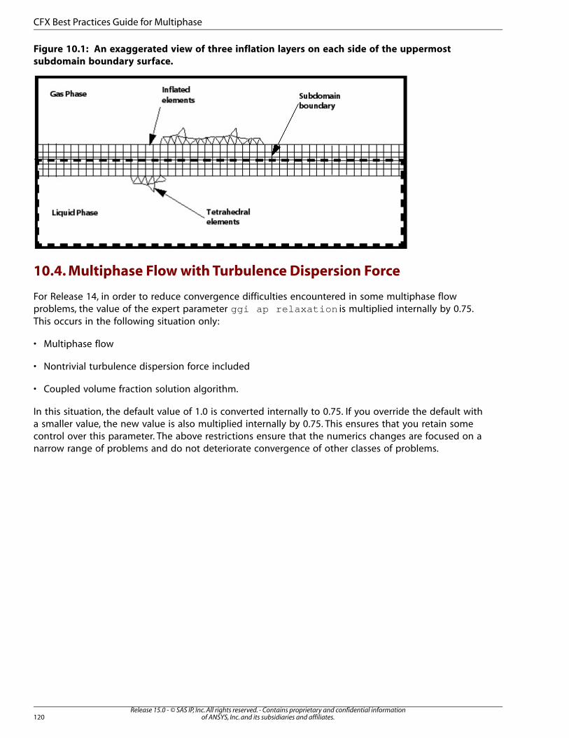
Figure 10.1: An exaggerated view of three inflation layers on each side of the uppermost
subdomain boundary surface.
10.4. Multiphase Flow with Turbulence Dispersion Force
For Release 14, in order to reduce convergence difficulties encountered in some multiphase flowproblems, the value of the expert parameter ggi ap relaxation is multiplied internally by 0.75.This occurs in the following situation only:
• Multiphase flow
• Nontrivial turbulence dispersion force included
• Coupled volume fraction solution algorithm.
In this situation, the default value of 1.0 is converted internally to 0.75. If you override the default witha smaller value, the new value is also multiplied internally by 0.75. This ensures that you retain somecontrol over this parameter. The above restrictions ensure that the numerics changes are focused on anarrow range of problems and do not deteriorate convergence of other classes of problems.
Release 15.0 - © SAS IP, Inc. All rights reserved. - Contains proprietary and confidential informationof ANSYS, Inc. and its subsidiaries and affiliates.120
CFX Best Practices Guide for Multiphase
Chapter 11: CFX Best Practices Guide for Turbomachinery
Turbomachinery applications can generally be divided into three main categories: gas compressors andturbines, liquid pumps and turbines, and fans and blowers. Each category is discussed in a separatesection below.
This guide describes best practices for setting up simulations involving:11.1. Gas Compressors and Turbines11.2. Liquid Pumps and Turbines11.3. Fans and Blowers11.4. Frame Change Models11.5. Domain Interface Setup
This guide is part of a series that provides advice for using CFX in specific engineering application areas.It is aimed at users with moderate or little experience using CFX for applications involving turboma-chinery.
11.1. Gas Compressors and Turbines
This section describes:
• Setup for Simulations of Gas Compressors and Turbines (p. 121)
• Convergence Tips (p. 122)
• Computing Speedlines for a Machine (p. 122)
• Post-Processing (p. 123)
11.1.1. Setup for Simulations of Gas Compressors and Turbines
Heat transfer and viscous work are involved, and can be modeled by using the Total Energy heattransfer model and enabling the Viscous Work Term option in CFX-Pre.
The industry-standard Shear Stress Transport model is the recommended choice for these cases. Whenusing the Shear Stress Transport model, ensure a resolution of the boundary layer of more than 10points. For details, see The k-omega and SST Models in the CFX-Solver Modeling Guide.
A common boundary condition configuration is to specify the total pressure and total temperature atthe inlet and either the mass flow, exit corrected mass flow, or static pressure at the outlet, dependingon the flow condition. Other configurations are also commonly used.
A good estimate of the timestep is within the region � to �, where � is the angular velocity ofthe rotating domain in radians per second. Selecting an automatic timestep will result in a timestep of
�.
The second-order high-resolution advection scheme is generally recommended.
121Release 15.0 - © SAS IP, Inc. All rights reserved. - Contains proprietary and confidential information
of ANSYS, Inc. and its subsidiaries and affiliates.
11.1.2. Convergence Tips
For high speed compressors and turbines, where the machine mass flow is choked, it is generally notpossible to specify the specified mass flow at the outlet to match the numerical choked mass flow value.For choked flow conditions, you can either specify static pressure or exit corrected mass flow at theoutlet. Both these conditions allow the mass flow through the machine to adjust to the numericalchoked mass flow value.
If you have trouble converging a simulation involving real gases, try to obtain a solution first using anideal gas. Ideal gases are available in the real gas library.
If you have trouble converging a problem with many stages, you may find that solving for a reducednumber of stages can give you a better understanding of the physics, and may allow you to restart amulti-stage problem with a better initial guess. You can also try ramping up boundary conditions andthe RPM.
Low pressure ratio Gas compressors (1.1 or less) can be treated more like liquid pumps. For details, seeLiquid Pumps and Turbines (p. 124).
11.1.3. Computing Speedlines for a Machine
Most turbomachinery simulations examine the machine performance across a range of operating points.A speedline involves varying the mass flow rate from choke to stall at a fixed rotational speed. This isoften accomplished by varying the exit mass flow rate or exit pressure while maintaining a constant,stationary frame total temperature and pressure at the inlet. If total conditions are not maintained atthe inlet, the resulting inlet mass flow rate must be corrected to a standard reference condition.
Performance along a speedline is typically measured in terms of a pressure ratio and an efficiency. Afull performance map is obtained by examining the performance across a range of rotation rates; thatis, multiple speedlines. A plot containing multiple speedlines is called the performance map of the ma-chine. Computing speedlines and performance maps requires many individual computations (one permass flow), therefore it is desirable to automate the process.
Depending on the machine type, you can use the following boundary conditions to effectively computespeedlines:
• For low speed compressors and turbines (subsonic), liquid pumps: Specify Total Pressure and Temper-
ature at the inlet and a Mass Flow Rate condition or a Exit Corrected Mass Flow Rate conditionat the outlet. This enables you to easily vary the mass flow across the full speedline while maintainingstationary inlet total conditions. For compressors, the specification of the mass flow rate at the outletis essential towards the low flow end of a speedline where the machine pressure ratio is insensitiveto the mass flow rate. For this reason, you should not specify a Static Pressure condition at theoutlet boundary for these machines.
• For high speed turbines and compressors (transonic): In these machines, the mass flow through thesystem is limited by a choked condition. If the specifed exit mass flow exceeds the choke flow rate,the net mass downstream of the choke condition will decrease until it reaches zero density, causingthe solver to fail. It is therefore important to avoid an exit mass flow near choke.
Similarly, at lower mass flow rates, close to stall, the pressure ratio is either constant or decreasing.A pressure specified outlet is generally unstable in this regime because there are multiple massflow rates which may satisfy the outlet condition. Therefore a pressure boundary condition shouldbe avoided in this range.
Release 15.0 - © SAS IP, Inc. All rights reserved. - Contains proprietary and confidential informationof ANSYS, Inc. and its subsidiaries and affiliates.122
CFX Best Practices Guide for Turbomachinery
This presents a problem with running speedlines using pressure and mass flow conditions, becauseneither boundary condition can be used across the entire speedline.
While the exit pressure and mass flow rate may be asymptotic over portions of a speedline, theexit corrected mass flow remains non-asymptotic and is therefore applicable across the entireoperating range. Thus, it is recommended that you use the Exit Corrected Mass Flow Rate
outlet boundary condition for running speedlines.
Some advantages of using the Exit Corrected Mass Flow Rate outlet boundary condition are:
• It allows you to specify the exit corrected mass flow, which is a function of the outlet mass flow rate, totalconditions, and a user-supplied reference condition.
• It makes it possible to automate the speedline analysis by enabling you to specify one boundary conditiontype that functions well across the entire speedline.
• It improves stability when a run is started with poor initial conditions, allowing for the use of a much largertimescale factor, so that all runs can be started from a simple or automatic initial guess. This allows pointsalong the speedline to be computed independently rather than using each existing solution to initializethe next.
• Typically in compressor operations, a fixed value of Exit Corrected Mass Flow Rate represents a fixedrunning or “op” line. As a result, you could keep the Exit Corrected Mass Flow Rate boundary conditionfixed and vary the rotational speed to generate the compressor performance along an op line. This isuseful when comparing designs.
For more details on the mathematical treatment of exit corrected mass flow rate as an outlet boundarycondition, see Exit Corrected Mass Flow Rate in the CFX-Solver Theory Guide.
11.1.4. Post-Processing
CFD-Post offers a powerful array of post-processing tools for turbomachinery applications, includingturbo-specific plots and performance calculation macros. To use many of the Turbo Post tools, you mustfirst initialize each domain by specifying the locations of turbo regions and instancing information.
The Turbo Calculator from the Turbo menu in CFD-Post allows you to perform calculations on the typeof application you are modeling. The macro prints a report in HTML showing a number of calculatedvariables, including torque, head and flow coefficients, blade loading, and efficiency.
You can also create your own macros to customize post-processing using Power Syntax, which is basedon the Perl language.
The optimal performance characteristics can be determined by creating a curve of pressure ratio versusflow rate.
123Release 15.0 - © SAS IP, Inc. All rights reserved. - Contains proprietary and confidential information
of ANSYS, Inc. and its subsidiaries and affiliates.
Gas Compressors and Turbines
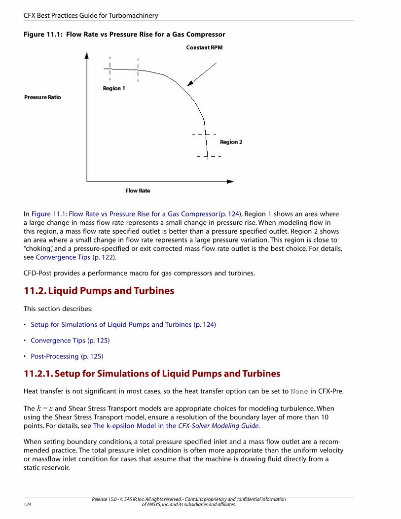
Figure 11.1: Flow Rate vs Pressure Rise for a Gas Compressor
In Figure 11.1: Flow Rate vs Pressure Rise for a Gas Compressor (p. 124), Region 1 shows an area wherea large change in mass flow rate represents a small change in pressure rise. When modeling flow inthis region, a mass flow rate specified outlet is better than a pressure specified outlet. Region 2 showsan area where a small change in flow rate represents a large pressure variation. This region is close to“choking”, and a pressure-specified or exit corrected mass flow rate outlet is the best choice. For details,see Convergence Tips (p. 122).
CFD-Post provides a performance macro for gas compressors and turbines.
11.2. Liquid Pumps and Turbines
This section describes:
• Setup for Simulations of Liquid Pumps and Turbines (p. 124)
• Convergence Tips (p. 125)
• Post-Processing (p. 125)
11.2.1. Setup for Simulations of Liquid Pumps and Turbines
Heat transfer is not significant in most cases, so the heat transfer option can be set to None in CFX-Pre.
The −� � and Shear Stress Transport models are appropriate choices for modeling turbulence. Whenusing the Shear Stress Transport model, ensure a resolution of the boundary layer of more than 10points. For details, see The k-epsilon Model in the CFX-Solver Modeling Guide.
When setting boundary conditions, a total pressure specified inlet and a mass flow outlet are a recom-mended practice. The total pressure inlet condition is often more appropriate than the uniform velocityor massflow inlet condition for cases that assume that the machine is drawing fluid directly from astatic reservoir.
Release 15.0 - © SAS IP, Inc. All rights reserved. - Contains proprietary and confidential informationof ANSYS, Inc. and its subsidiaries and affiliates.124
CFX Best Practices Guide for Turbomachinery
As with gas compressors, a good estimate of the timestep is within the region � to �, where �is the angular velocity of the rotating domain in radians per second. Selecting an automatic timestep
will result in a timestep of �.
The high-resolution advection scheme is recommended.
This document deals with obtaining solutions for cases without cavitation, but cavitation may be present.For advice on how to deal with cavitation, see CFX Best Practices Guide for Cavitation (p. 105).
11.2.2. Convergence Tips
When only a poor initial guess is available, it may be helpful to first run with a specified mass flow inletand a static pressure outlet. The outlet pressure in this case is fairly arbitrary and is usually set at, orclose to zero to reduce round-off error. The specification of a mass flow inlet may be more robust.However, a mass flow inlet assumes a uniform inlet velocity which may not be appropriate. Once theoverall flow is established, the boundary conditions may then be changed to total pressure at the inletand mass flow at the outlet.
11.2.3. Post-Processing
If a total pressure inlet boundary condition is used (recommended where possible), it will also providea useful starting point for streamlines that are colored by total pressure during post-processing. Theuniform total pressure distribution means lines will begin with a uniform color. It may be harder tovisually resolve these pressure values if an inlet velocity profile is used.
CFD-Post provides a performance macro for liquid pumps and turbines.
11.3. Fans and Blowers
This section describes:
• Setup for Simulations of Fans and Blowers (p. 125)
• Convergence Tips (p. 125)
• Post-Processing (p. 126)
11.3.1. Setup for Simulations of Fans and Blowers
Fans and blowers behave like liquid pumps, and require a similar model setup. The flow is generallymodeled as incompressible and isothermal. The fluid is typically air as a general fluid or as an ideal gas
at a specified temperature. The −� � or SST model is used to model turbulence.
Boundary conditions, turbulence models and choice of timestep are the same as for liquid pumps andturbines.
11.3.2. Convergence Tips
The use of the alternate rotation model is an important consideration when modeling fans and blowers.Where long axisymmetric inlets exist, the absolute frame velocity has less swirl than the relative framevelocity. Because the alternate rotation model solves for the absolute frame velocity, it can reduce nu-merical error in such inlet sections. The model may introduce errors in the exit stream if the flow ishighly swirling. Hence, the length of the inlet and exit sections can be an important factor when
125Release 15.0 - © SAS IP, Inc. All rights reserved. - Contains proprietary and confidential information
of ANSYS, Inc. and its subsidiaries and affiliates.
Fans and Blowers
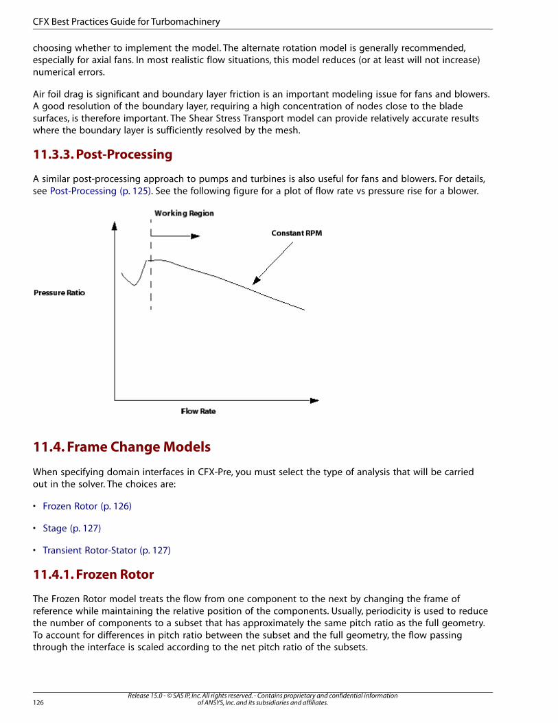
choosing whether to implement the model. The alternate rotation model is generally recommended,especially for axial fans. In most realistic flow situations, this model reduces (or at least will not increase)numerical errors.
Air foil drag is significant and boundary layer friction is an important modeling issue for fans and blowers.A good resolution of the boundary layer, requiring a high concentration of nodes close to the bladesurfaces, is therefore important. The Shear Stress Transport model can provide relatively accurate resultswhere the boundary layer is sufficiently resolved by the mesh.
11.3.3. Post-Processing
A similar post-processing approach to pumps and turbines is also useful for fans and blowers. For details,see Post-Processing (p. 125). See the following figure for a plot of flow rate vs pressure rise for a blower.
11.4. Frame Change Models
When specifying domain interfaces in CFX-Pre, you must select the type of analysis that will be carriedout in the solver. The choices are:
• Frozen Rotor (p. 126)
• Stage (p. 127)
• Transient Rotor-Stator (p. 127)
11.4.1. Frozen Rotor
The Frozen Rotor model treats the flow from one component to the next by changing the frame ofreference while maintaining the relative position of the components. Usually, periodicity is used to reducethe number of components to a subset that has approximately the same pitch ratio as the full geometry.To account for differences in pitch ratio between the subset and the full geometry, the flow passingthrough the interface is scaled according to the net pitch ratio of the subsets.
Release 15.0 - © SAS IP, Inc. All rights reserved. - Contains proprietary and confidential informationof ANSYS, Inc. and its subsidiaries and affiliates.126
CFX Best Practices Guide for Turbomachinery
The Frozen Rotor model must be used for non-axisymmetric flow domains, such as impeller/volute,turbine/draft tube, propeller/ship and scroll/volute cases. It can also be used for axial compressors andturbines. The Frozen Rotor model has the advantages of being robust, using less computer resourcesthan the other frame change models, and being well suited for high blade counts. The drawbacks ofthe model include inadequate prediction of physics for local flow values and sensitivity of the resultsto the relative position of the rotor and stator for tightly coupled components.
11.4.2. Stage
The Stage model circumferentially averages the fluxes in bands and transmits the average fluxes to thedownstream component. Possible applications include axial turbines, compressors and pumps, as wellas fans and torque converters. The model is useful for large pitch ratios and still takes a relatively shorttime to solve. The model is not suitable for applications with tight coupling of components and/orsignificant wake interaction effects and may not accurately predict loading.
11.4.3. Transient Rotor-Stator
The Transient Rotor-Stator model takes into account all of the transient flow characteristics. A slidinginterface is used to allow a smooth rotation between components. As with the Frozen Rotor model, theTransient Rotor-Stator model scales the flow from one component to the next in order to account fora non-unity net pitch ratio. This model is robust and yields high accuracy predictions of loading. Thedrawbacks include high computational cost and large amounts of storage required to hold the transientdata.
Note
The dynamic re-intersection of the interface at the start of each time step may result in adifferent interface topology, which in turn may require more or less memory. Unlike thestatic interfaces (Frozen Rotor, Stage), which are only intersected once (first time step of aserial run or partitioner in a parallel run), the initial memory estimate might not be sufficientfor the whole run. To avoid potential memory problems, it might be necessary to start thesimulation with more conservative (larger) memory factors.
11.5. Domain Interface Setup
The setup of domain interfaces is an important consideration when defining a problem. The followingsection outlines some approved practices for use in turbomachinery applications.
11.5.1. General Considerations
• Domain interfaces should typically be placed midway between the rotor and stator for turbomachinerycases.
• To avoid numerical errors, the aspect ratio of elements on the domain interface should be between 0.1:1and 10:1, as measured by x/y in Figure 11.2: Element Aspect Ratio at Domain Interface (p. 128).
• Where circular domain interfaces exist, they must be axisymmetric in shape as shown in Figure 11.3: Im-peller/Volute (p. 128).
127Release 15.0 - © SAS IP, Inc. All rights reserved. - Contains proprietary and confidential information
of ANSYS, Inc. and its subsidiaries and affiliates.
Domain Interface Setup
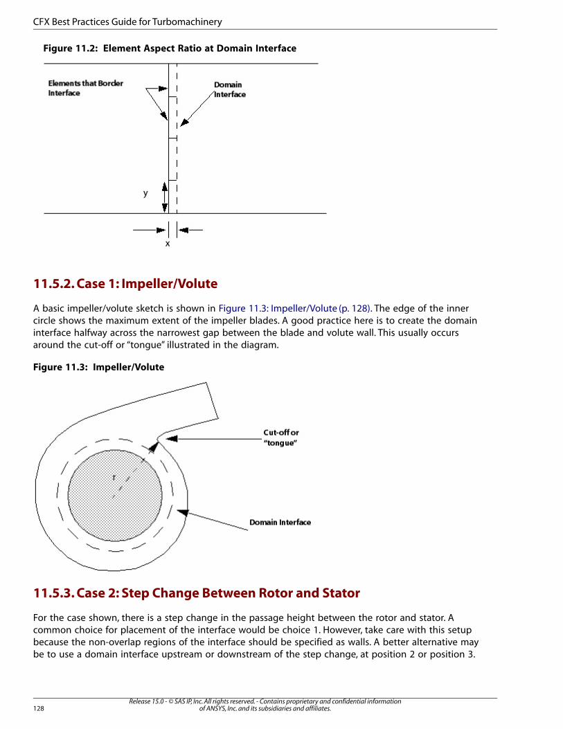
Figure 11.2: Element Aspect Ratio at Domain Interface
11.5.2. Case 1: Impeller/Volute
A basic impeller/volute sketch is shown in Figure 11.3: Impeller/Volute (p. 128). The edge of the innercircle shows the maximum extent of the impeller blades. A good practice here is to create the domaininterface halfway across the narrowest gap between the blade and volute wall. This usually occursaround the cut-off or “tongue” illustrated in the diagram.
Figure 11.3: Impeller/Volute
11.5.3. Case 2: Step Change Between Rotor and Stator
For the case shown, there is a step change in the passage height between the rotor and stator. Acommon choice for placement of the interface would be choice 1. However, take care with this setupbecause the non-overlap regions of the interface should be specified as walls. A better alternative maybe to use a domain interface upstream or downstream of the step change, at position 2 or position 3.
Release 15.0 - © SAS IP, Inc. All rights reserved. - Contains proprietary and confidential informationof ANSYS, Inc. and its subsidiaries and affiliates.128
CFX Best Practices Guide for Turbomachinery
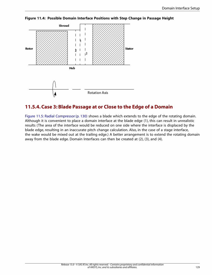
Figure 11.4: Possible Domain Interface Positions with Step Change in Passage Height
11.5.4. Case 3: Blade Passage at or Close to the Edge of a Domain
Figure 11.5: Radial Compressor (p. 130) shows a blade which extends to the edge of the rotating domain.Although it is convenient to place a domain interface at the blade edge (1), this can result in unrealisticresults (The area of the interface would be reduced on one side where the interface is displaced by theblade edge, resulting in an inaccurate pitch change calculation. Also, in the case of a stage interface,the wake would be mixed out at the trailing edge.) A better arrangement is to extend the rotating domainaway from the blade edge. Domain Interfaces can then be created at (2), (3), and (4).
129Release 15.0 - © SAS IP, Inc. All rights reserved. - Contains proprietary and confidential information
of ANSYS, Inc. and its subsidiaries and affiliates.
Domain Interface Setup
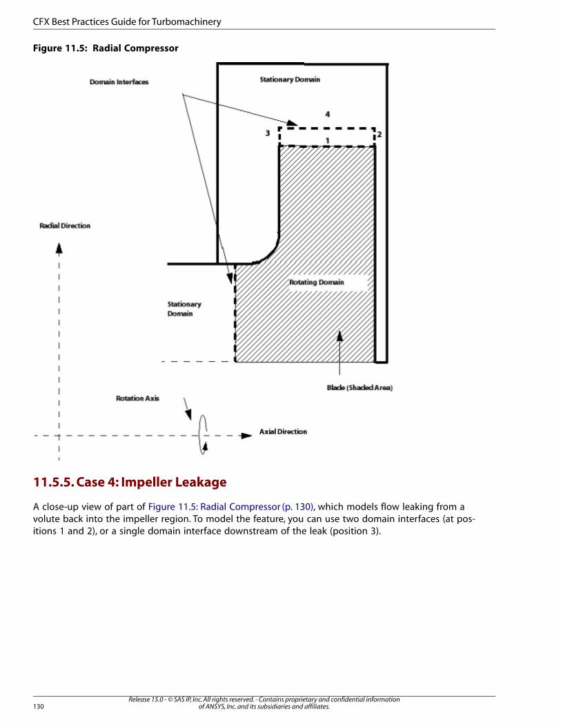
Figure 11.5: Radial Compressor
11.5.5. Case 4: Impeller Leakage
A close-up view of part of Figure 11.5: Radial Compressor (p. 130), which models flow leaking from avolute back into the impeller region. To model the feature, you can use two domain interfaces (at pos-itions 1 and 2), or a single domain interface downstream of the leak (position 3).
Release 15.0 - © SAS IP, Inc. All rights reserved. - Contains proprietary and confidential informationof ANSYS, Inc. and its subsidiaries and affiliates.130
CFX Best Practices Guide for Turbomachinery
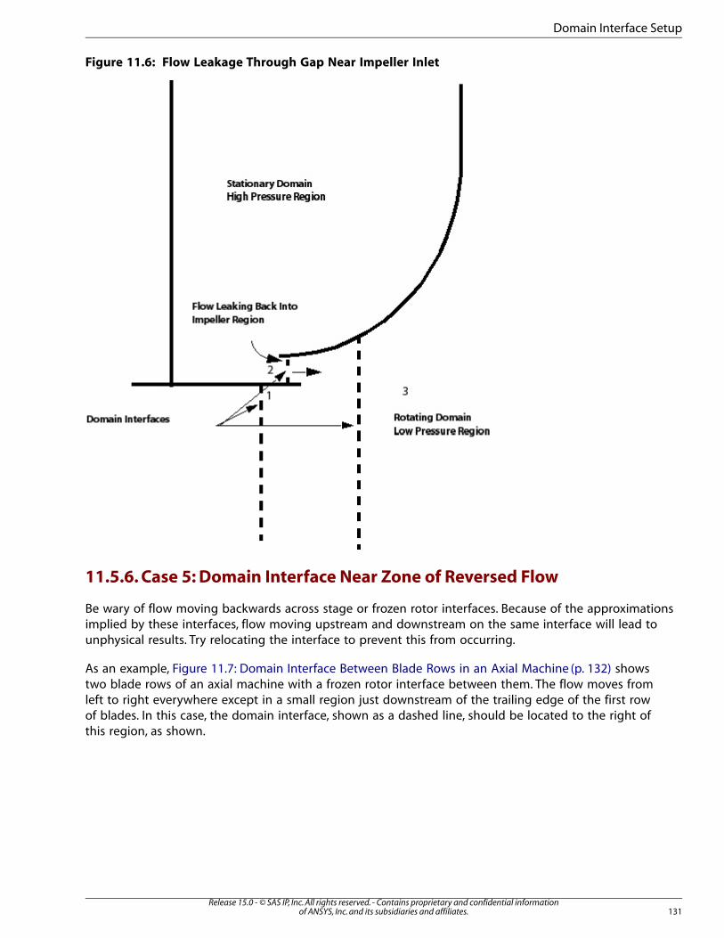
Figure 11.6: Flow Leakage Through Gap Near Impeller Inlet
11.5.6. Case 5: Domain Interface Near Zone of Reversed Flow
Be wary of flow moving backwards across stage or frozen rotor interfaces. Because of the approximationsimplied by these interfaces, flow moving upstream and downstream on the same interface will lead tounphysical results. Try relocating the interface to prevent this from occurring.
As an example, Figure 11.7: Domain Interface Between Blade Rows in an Axial Machine (p. 132) showstwo blade rows of an axial machine with a frozen rotor interface between them. The flow moves fromleft to right everywhere except in a small region just downstream of the trailing edge of the first rowof blades. In this case, the domain interface, shown as a dashed line, should be located to the right ofthis region, as shown.
131Release 15.0 - © SAS IP, Inc. All rights reserved. - Contains proprietary and confidential information
of ANSYS, Inc. and its subsidiaries and affiliates.
Domain Interface Setup

Figure 11.7: Domain Interface Between Blade Rows in an Axial Machine
Release 15.0 - © SAS IP, Inc. All rights reserved. - Contains proprietary and confidential informationof ANSYS, Inc. and its subsidiaries and affiliates.132
CFX Best Practices Guide for Turbomachinery
Chapter 12: Best Practice: Scale-Resolving Simulations in ANSYS
CFD
12.1. Introduction
While today’s CFD simulations are mainly based on Reynolds-Averaged Navier-Stokes (RANS) turbulencemodels, it is becoming increasingly clear that certain classes of flows are better covered by models inwhich all or a part of the turbulence spectrum is resolved in at least a portion of the numerical domain.Such methods are termed Scale-Resolving Simulation (SRS) models in this paper.
There are two main motivations for using SRS models in favor of RANS formulations. The first reasonfor using SRS models is the need for additional information that cannot be obtained from the RANSsimulation. Examples are acoustics simulations where the turbulence generates noise sources, whichcannot be extracted with accuracy from RANS simulations. Other examples are unsteady heat loadingin unsteady mixing zones of flow streams at different temperatures, which can lead to material failure,or multi-physics effects like vortex cavitation, where the unsteady turbulence pressure field is the causeof cavitation. In such situations, the need for SRS can exist even in cases where the RANS model wouldin principle be capable of computing the correct time-averaged flow field.
The second reason for using SRS models is related to accuracy. It is known that RANS models have theirlimitations in accuracy in certain flow situations. RANS models have shown their strength essentiallyfor wall-bounded flows, where the calibration according to the law-of-the-wall provides a soundfoundation for further refinement. For free shear flows, the performance of RANS models is much lessuniform. There is a wide variety of such flows, ranging from simple self-similar flows such as jets, mixinglayers, and wakes to impinging flows, flows with strong swirl, massively separated flows, and manymore. Considering that RANS models typically already have limitations covering the most basic self-similar free shear flows with one set of constants, there is little hope that even the most advancedReynolds Stress Models (RSM) will eventually be able to provide a reliable foundation for all such flows.(For an overview of RANS modeling, see Durbin, Pettersson and Reif, 2003 [5] (p. 207); Wilcox, 2006[38] (p. 209); or Hanjalic and Launder, 2011 [13] (p. 208).)
For free shear flows, it is typically much easier to resolve the largest turbulence scales, as they are ofthe order of the shear layer thickness. In contrast, in wall boundary layers the turbulence length scalenear the wall becomes very small relative to the boundary layer thickness (increasingly so at higher Renumbers). This poses severe limitations for Large Eddy Simulation (LES) as the computational effort re-quired is still far from the computing power available to industry (Spalafrt, 1997 [29] (p. 209)). (For anoverview of LES modeling, see Guerts, 2004 [12] (p. 208), and Wagner et al., 2007 [35] (p. 209).) For thisreason, hybrid models are under development where large eddies are resolved only away from wallsand the wall boundary layers are covered by a RANS model. Examples of such global hybrid modelsare Detached Eddy Simulation (DES, see Spalart, 2000 [30] (p. 209)) or Scale-Adaptive Simulation (SAS,see Menter and Egorov, 2010 [18] (p. 208)). A further step is to apply a RANS model only in the innermostpart of the wall boundary layer and then to switch to a LES model for the main part of the boundarylayer. Such models are termed Wall-modeled LES (WMLES) (see Shur et al., 2008 [26] (p. 208)). Finally,for large domains, it is frequently necessary to cover only a small portion with SRS models, while themajority of the flow can be computed in RANS mode. In such situations, zonal or embedded LESmethods are attractive as they enable you to specify ahead of time the region where LES is required.
133Release 15.0 - © SAS IP, Inc. All rights reserved. - Contains proprietary and confidential information
of ANSYS, Inc. and its subsidiaries and affiliates.
Such methods are typically not new models in the strict sense, but enable the combination of existingmodels/technologies in a flexible way in different portions of the flowfield. Important elements ofzonal models are interface conditions, which convert turbulence from RANS mode to resolved modeat pre-defined locations. In most cases, this is achieved by introducing synthetic turbulence based onthe length and time scales from the RANS model.
There are many hybrid RANS-LES models, often with somewhat confusing naming conventions, thatvary in the range of turbulence eddies they can resolve. On close inspection, many of these models areonly slight variations of the Detached Eddy Simulation (DES) concept of Spalart, 2000 [30] (p. 209) andhave very similar performance. For a general overview of SRS modeling concepts, see Fröhlich and vonTerzi, 2008 [8] (p. 207), and Sagaut et al., 2006 [24] (p. 208).
SRS models are very challenging in their proper application to industrial flows. The models typicallyrequire special attention to various details such as:
• Model selection
• Grid generation
• Numerical settings
• Solution interpretation
• Post-processing
• Quality assurance
Unfortunately, there is no unique model covering all industrial flows, and each individual model posesits own set of challenges. In general, when using a CFD code, you must understand the intricacies ofthe SRS model formulation in order to be able to select the optimal model and to use it efficiently. Thisreport is intended to support you in the basic understanding of such models and to provide bestpractice guidelines for their usage. The discussion is focused on the models available in the ANSYS CFDsoftware.
This report is intended as an addition to the code-specific Theory and User Documentation availablefor both ANSYS Fluent and ANSYS CFX . The Theory and User Documentation describes in detail howto select and activate these models, so that information is not repeated here. This report is intendedto provide you with a general understanding of the underlying principles and the associated limitationsof each of the described modeling concepts. It also covers the types of flows for which the models aresuitable as well as flows where they will likely not work well. Finally, the impact of numerical settingson model performance is discussed.
In accordance with the intention of providing you with recommendations for your day-to-day work,several Appendices can be found at the end of the document for quick reference of the most importantpoints.
12.2. General Aspects
This chapter discusses:12.2.1. Limitations of Large Eddy Simulation (LES)
Release 15.0 - © SAS IP, Inc. All rights reserved. - Contains proprietary and confidential informationof ANSYS, Inc. and its subsidiaries and affiliates.134
Best Practice: Scale-Resolving Simulations in ANSYS CFD
12.2.1. Limitations of Large Eddy Simulation (LES)
In order to understand the motivation for hybrid models, one has to discuss the limitations of LargeEddy Simulation (LES). LES has been the most widely used SRS model over the last decades. It is basedon the concept of resolving only the large scales of turbulence and to model the small scales. Theclassical motivation for LES is that the large scales are problem-dependent and difficult to model,whereas the smaller scales become more and more universal and isotropic and can be modeled moreeasily.
LES is based on filtering the Navier-Stokes equations over a finite spatial region (typically the gridvolume) and aimed at only resolving the portions of turbulence larger than the filter width. Turbulencestructures smaller than the filter are then modeled, typically by a simple Eddy Viscosity model.
The filtering operation is defined as:
(12.1)
ur ur ur ur
ur ur ur
∫
∫
= ′ − ′
− ′ ′ =
− ∞
∞
− ∞
∞
� � � � � � � �
� � � � �
where � is the spatial filter. Filtering the Navier-Stokes equations results in the following form (densityfluctuations neglected):
(12.2)∂
∂+
∂∂
= − ∂∂
+ ∂∂
+��
�
�� �
�
� �
� � �
� � ��� ��
��
The equations feature an additional stress term due to the filtering operation:
(12.3)= −� �� � �� ������
� � � �
Despite the difference in derivation, the additional sub-grid stress tensor is typically modeled as in RANSusing an eddy viscosity model:
(12.4)=
∂∂
+∂∂
� �
�
�
�
�����
!�
�
�
�
The important practical implication from this modeling approach is that the modeled momentumequations for RANS and LES are identical if an eddy-viscosity model is used in both cases. The modeledNavier-Stokes equations have no knowledge of their derivation. The only information they obtain fromthe turbulence model is the size of the eddy viscosity. Depending on that, the equations will operatein RANS or LES mode (or in some intermediate mode). The formal identity of the filtered Navier-Stokesand the RANS equations is the basis of hybrid RANS-LES turbulence models, which can obviously beintroduced into the same set of momentum equations. Only the model (and the numerics) have to beswitched.
Classical LES models are of the form of the Smagorinsky, 1963 [28] (p. 209) model:
(12.5)=" # $ %& '
(
135Release 15.0 - © SAS IP, Inc. All rights reserved. - Contains proprietary and confidential information
of ANSYS, Inc. and its subsidiaries and affiliates.
General Aspects
where is a measure of the grid spacing of the numerical mesh, � is the strain rate scalar and �� isa constant. This is obviously a rather simple formulation, indicating that LES models will not provide ahighly accurate representation of the smallest scales. From a practical standpoint, a very detailedmodeling might not be required. A more appropriate goal for LES is not to model the impact of theunresolved scales onto the resolved ones, but to model the dissipation of the smallest resolved scales.This can be seen from Figure 12.1 (p. 137) showing the turbulence energy spectrum of a Decaying Iso-tropic Turbulence (DIT) test case, i.e. initially stirred turbulence in a box, decaying over time (Comte-
Bellot and Corrsin, 1971 [3] (p. 207)). � � is the turbulence energy as a function of wave number �.Small � values represent large eddies and large � values represent small eddies. Turbulence movesdown the turbulence spectrum from the small wave number to the high wave numbers. In a fully resolvedsimulation (Direct Numerical Simulation, or DNS), the turbulence is dissipated into heat at the smallest
scales ( ∼� in Figure 12.1 (p. 137)), by viscosity. The dissipation is achieved by:
(12.6)= ∂∂
∂∂
�
�
�
� ��
�
�
�
�
where � is typically a very small kinematic molecular viscosity. The dissipation � ��� is still of finitevalue as the velocity gradients of the smallest scales are very large.
LES computations are usually performed on numerical grids that are too coarse to resolve the smallestscales. In the current example, the cut-off limit of LES (resolution limit) is at around =� . The velocitygradients of the smallest resolved scales in LES are therefore much smaller than those at the DNS limit.The molecular viscosity is then not sufficient to provide the correct level of dissipation. In this case, theproper amount of dissipation can be achieved by increasing the viscosity, using an eddy-viscosity:
(12.7)= ∂∂
∂∂
� ��
�
�
���� �
!
!
The eddy viscosity is calibrated to provide the correct amount of dissipation at the LES grid limit. Theeffect can be seen in Figure 12.1 (p. 137), where a LES of the DIT case is performed without a LES modeland with different LES models. When the LES models are activated, the energy is dissipated and themodels provide a sensible spectrum for all resolved scales. LES is not modeling the influence of unresolvedsmall scale turbulence onto the larger, resolved scales, but the dissipation of turbulence into heat (thedissipated energy is typically very small relative to the thermal energy of the fluid and does not haveto be accounted for, except for high Mach number flows).
Release 15.0 - © SAS IP, Inc. All rights reserved. - Contains proprietary and confidential informationof ANSYS, Inc. and its subsidiaries and affiliates.136
Best Practice: Scale-Resolving Simulations in ANSYS CFD

Figure 12.1: Turbulence spectrum for DIT test case after t=2. Comparison of results without
Sub-Grid Scale model (no LES) with WALE and Smagorinsky LES model simulations
This discussion shows that LES is a fairly simple technology, which does not provide a reliable backbonefor modeling. This is also true for more complex LES models like dynamic models. Dynamic eddy viscosityLES models (see Guerts, 2004 [12] (p. 208)) are designed to estimate the required level of dissipation atthe grid limit from flow conditions at larger scales (typically twice the filter width), thereby reducingthe need for model calibration. Such models, however, also only provide a suitable eddy viscosity levelfor energy dissipation. Within the LES framework, all features and effects of the flow that are of interestand relevance to engineers have to be resolved in space and time. This requirement makes LES inprinciple a very CPU-expensive technology.
Even more demanding is the application of LES to wall-bounded flows, which is the typical situation inengineering flows. The turbulent length scale,�, of the large eddies can be expressed as:
(12.8)=� ��
where � is the wall distance and � a constant. Even the (locally) largest scales become very small nearthe wall and require a high resolution in all three space dimensions and in time.
The linear dependence of � on � indicates that the turbulence length scales approach zero near thewall, which would require an infinitely fine grid to resolve them. This is not the case in reality, as themolecular viscosity prevents scales smaller than the Kolmogorov limit. This is manifested by the viscousor laminar sublayer, a region very close to the wall, where turbulence is damped and does not need tobe resolved. However, the viscous sublayer thickness is a function of the Reynolds number, Re, of theflow. At higher Re numbers, the viscous sublayer becomes decreasingly thinner and thereby allows the
137Release 15.0 - © SAS IP, Inc. All rights reserved. - Contains proprietary and confidential information
of ANSYS, Inc. and its subsidiaries and affiliates.
General Aspects
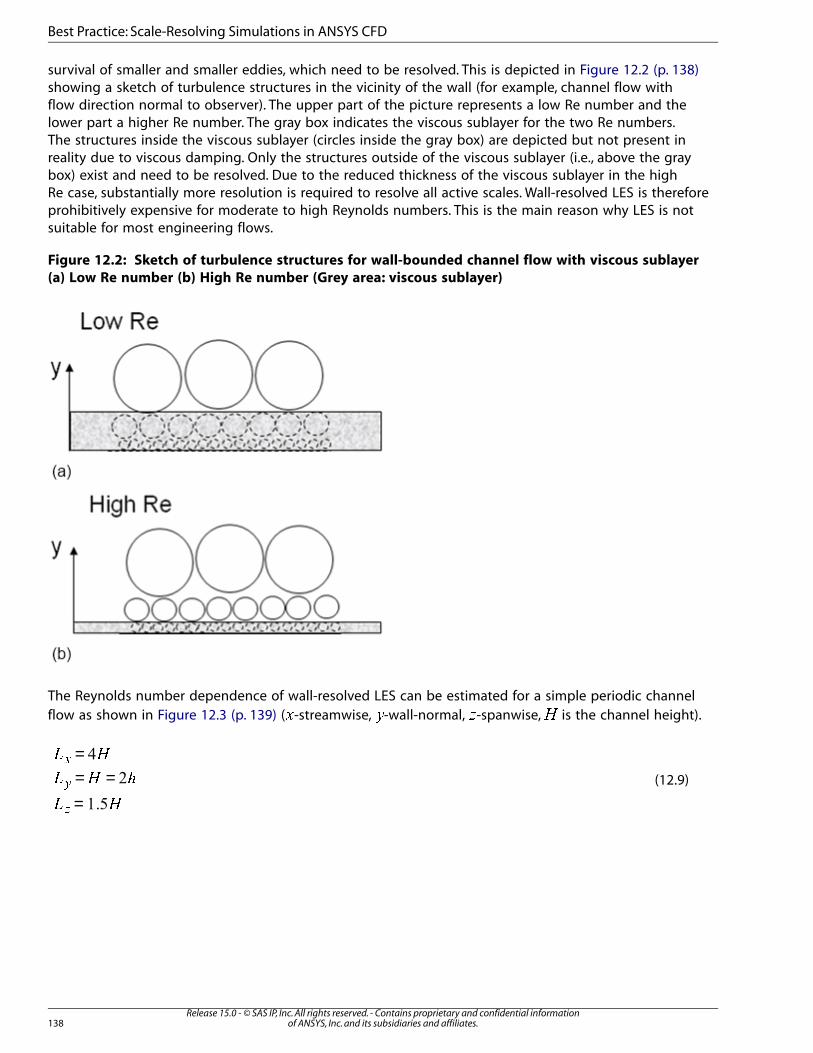
survival of smaller and smaller eddies, which need to be resolved. This is depicted in Figure 12.2 (p. 138)showing a sketch of turbulence structures in the vicinity of the wall (for example, channel flow withflow direction normal to observer). The upper part of the picture represents a low Re number and thelower part a higher Re number. The gray box indicates the viscous sublayer for the two Re numbers.The structures inside the viscous sublayer (circles inside the gray box) are depicted but not present inreality due to viscous damping. Only the structures outside of the viscous sublayer (i.e., above the graybox) exist and need to be resolved. Due to the reduced thickness of the viscous sublayer in the highRe case, substantially more resolution is required to resolve all active scales. Wall-resolved LES is thereforeprohibitively expensive for moderate to high Reynolds numbers. This is the main reason why LES is notsuitable for most engineering flows.
Figure 12.2: Sketch of turbulence structures for wall-bounded channel flow with viscous sublayer
(a) Low Re number (b) High Re number (Grey area: viscous sublayer)
The Reynolds number dependence of wall-resolved LES can be estimated for a simple periodic channelflow as shown in Figure 12.3 (p. 139) (�-streamwise, �-wall-normal, �-spanwise, � is the channel height).
(12.9)
== ==
� �
� � �
� �
�
�
Release 15.0 - © SAS IP, Inc. All rights reserved. - Contains proprietary and confidential informationof ANSYS, Inc. and its subsidiaries and affiliates.138
Best Practice: Scale-Resolving Simulations in ANSYS CFD
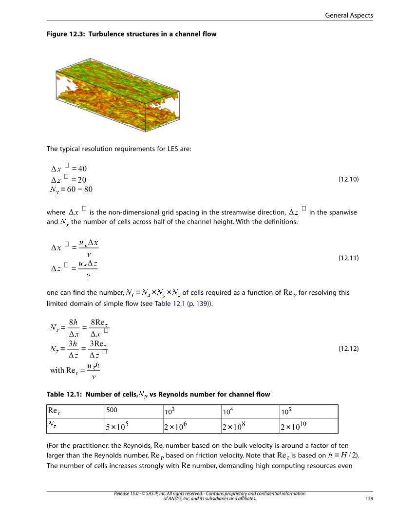
Figure 12.3: Turbulence structures in a channel flow
The typical resolution requirements for LES are:
(12.10)
==
= −
+
+�
�
��
where +
� is the non-dimensional grid spacing in the streamwise direction,+
� in the spanwiseand �� the number of cells across half of the channel height. With the definitions:
(12.11)
=
=
+
+
� �
� �
�
�
one can find the number, = × × � � � � of cells required as a function of �, for resolving this
limited domain of simple flow (see Table 12.1 (p. 139)).
(12.12)
= =
= =
=
+
+
��
� �
��
� �
� �
�
��
��
��
Table 12.1: Number of cells,��, vs Reynolds number for channel flow
105104103500�
× � × !× "× #$%
(For the practitioner: the Reynolds, , number based on the bulk velocity is around a factor of ten
larger than the Reynolds number, &, based on friction velocity. Note that ' is based on =( ) ).
The number of cells increases strongly with number, demanding high computing resources even
139Release 15.0 - © SAS IP, Inc. All rights reserved. - Contains proprietary and confidential information
of ANSYS, Inc. and its subsidiaries and affiliates.
General Aspects
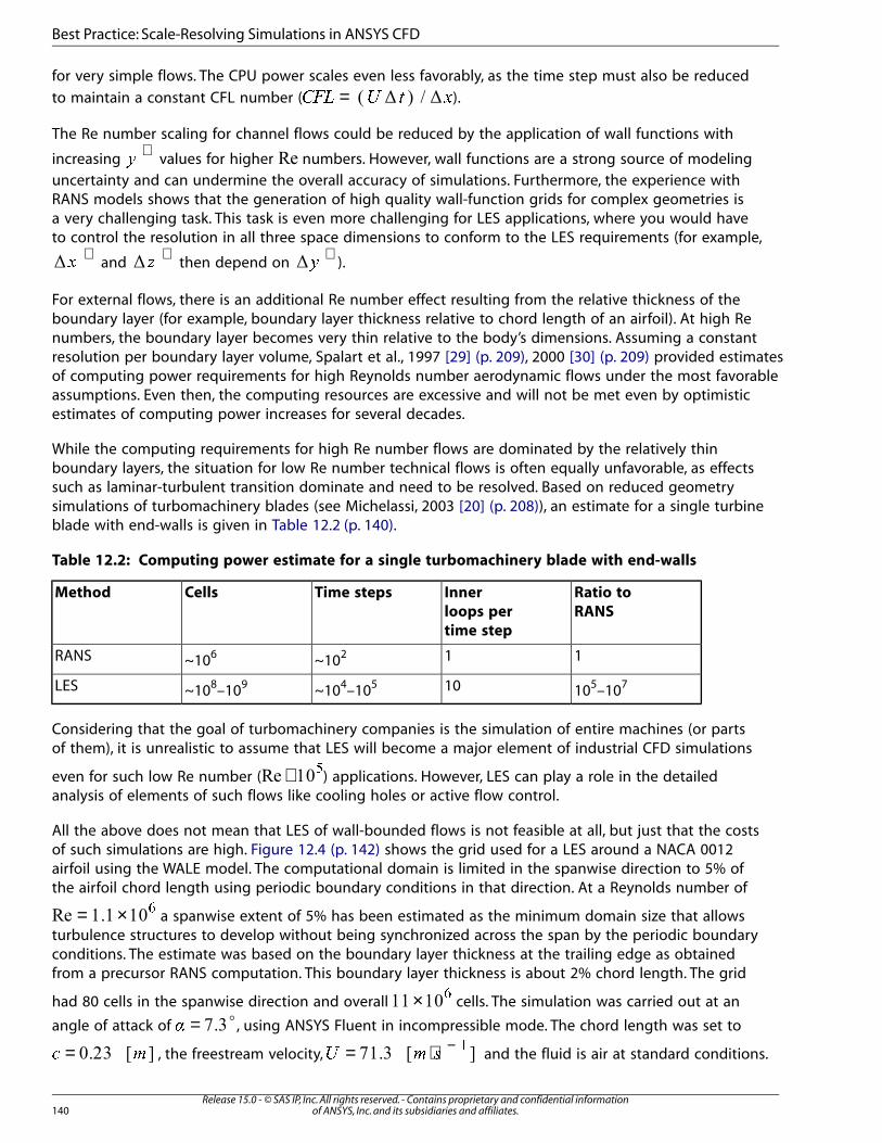
for very simple flows. The CPU power scales even less favorably, as the time step must also be reduced
to maintain a constant CFL number ( =��� � � �).
The Re number scaling for channel flows could be reduced by the application of wall functions with
increasing +
� values for higher numbers. However, wall functions are a strong source of modelinguncertainty and can undermine the overall accuracy of simulations. Furthermore, the experience withRANS models shows that the generation of high quality wall-function grids for complex geometries isa very challenging task. This task is even more challenging for LES applications, where you would haveto control the resolution in all three space dimensions to conform to the LES requirements (for example,
+� and
+� then depend on
+ ).
For external flows, there is an additional Re number effect resulting from the relative thickness of theboundary layer (for example, boundary layer thickness relative to chord length of an airfoil). At high Renumbers, the boundary layer becomes very thin relative to the body’s dimensions. Assuming a constantresolution per boundary layer volume, Spalart et al., 1997 [29] (p. 209), 2000 [30] (p. 209) provided estimatesof computing power requirements for high Reynolds number aerodynamic flows under the most favorableassumptions. Even then, the computing resources are excessive and will not be met even by optimisticestimates of computing power increases for several decades.
While the computing requirements for high Re number flows are dominated by the relatively thinboundary layers, the situation for low Re number technical flows is often equally unfavorable, as effectssuch as laminar-turbulent transition dominate and need to be resolved. Based on reduced geometrysimulations of turbomachinery blades (see Michelassi, 2003 [20] (p. 208)), an estimate for a single turbineblade with end-walls is given in Table 12.2 (p. 140).
Table 12.2: Computing power estimate for a single turbomachinery blade with end-walls
Ratio to
RANS
Inner
loops per
time step
Time stepsCellsMethod
11~102~106RANS
105–10710~104–105~108–109LES
Considering that the goal of turbomachinery companies is the simulation of entire machines (or partsof them), it is unrealistic to assume that LES will become a major element of industrial CFD simulations
even for such low Re number ( ∼ ) applications. However, LES can play a role in the detailed
analysis of elements of such flows like cooling holes or active flow control.
All the above does not mean that LES of wall-bounded flows is not feasible at all, but just that the costsof such simulations are high. Figure 12.4 (p. 142) shows the grid used for a LES around a NACA 0012airfoil using the WALE model. The computational domain is limited in the spanwise direction to 5% ofthe airfoil chord length using periodic boundary conditions in that direction. At a Reynolds number of
= × � a spanwise extent of 5% has been estimated as the minimum domain size that allows
turbulence structures to develop without being synchronized across the span by the periodic boundaryconditions. The estimate was based on the boundary layer thickness at the trailing edge as obtainedfrom a precursor RANS computation. This boundary layer thickness is about 2% chord length. The grid
had 80 cells in the spanwise direction and overall × � cells. The simulation was carried out at an
angle of attack of o= , using ANSYS Fluent in incompressible mode. The chord length was set to
=� � , the freestream velocity, = ⋅ −� � �
� and the fluid is air at standard conditions.
Release 15.0 - © SAS IP, Inc. All rights reserved. - Contains proprietary and confidential informationof ANSYS, Inc. and its subsidiaries and affiliates.140
Best Practice: Scale-Resolving Simulations in ANSYS CFD
The time step was set to = × −� �
� giving a Courant number of ∼��� inside the
boundary layer. Figure 12.5 (p. 143) shows turbulence structures near the leading edge (a) and thetrailing edge (b). Near the leading edge, the laminar-turbulent transition can clearly be seen. Thetransition is triggered by a laminar separation bubble. Near the trailing edge, the turbulence structuresare already relatively large, but still appear unsynchronized in the spanwise direction (no large scale 2D
structures with axis orientation in the spanwise direction). The simulation was run for ~104 time steps
before the averaging procedure was started. The time averaging was conducted for ∼ × � time
steps. Figure 12.6 (p. 143) shows a comparison of the wall pressure coefficient �� and Figure 12.7 (p. 144)
of the wall shear stress coefficient on the suction side of the airfoil in comparison to a RANS compu-
tation using the SST model (Menter, 1994 [16] (p. 208)). No detailed discussion of the simulation is inten-ded here, but the comparison of the wall shear stress with the well-calibrated RANS model indicatesthat the resolution of the grid is still insufficient for capturing the near-wall details. For this reason, thewall shear stress is significantly underestimated by about 30% compared to the SST model in the leadingedge area. As the trailing edge is approached, the comparison improves, mainly because the boundarylayer thickness is increased whereas the wall shear stress is decreased, which produces a higher relativeresolution in the LES. Based on this simulation, it is estimated that a refinement by a factor of 2, in bothstreamwise and spanwise directions, would be required in order to reproduce the correct wall shearstress. While such a resolution is not outside the realm of available computers, it is still far too high forday-to-day simulations.
141Release 15.0 - © SAS IP, Inc. All rights reserved. - Contains proprietary and confidential information
of ANSYS, Inc. and its subsidiaries and affiliates.
General Aspects
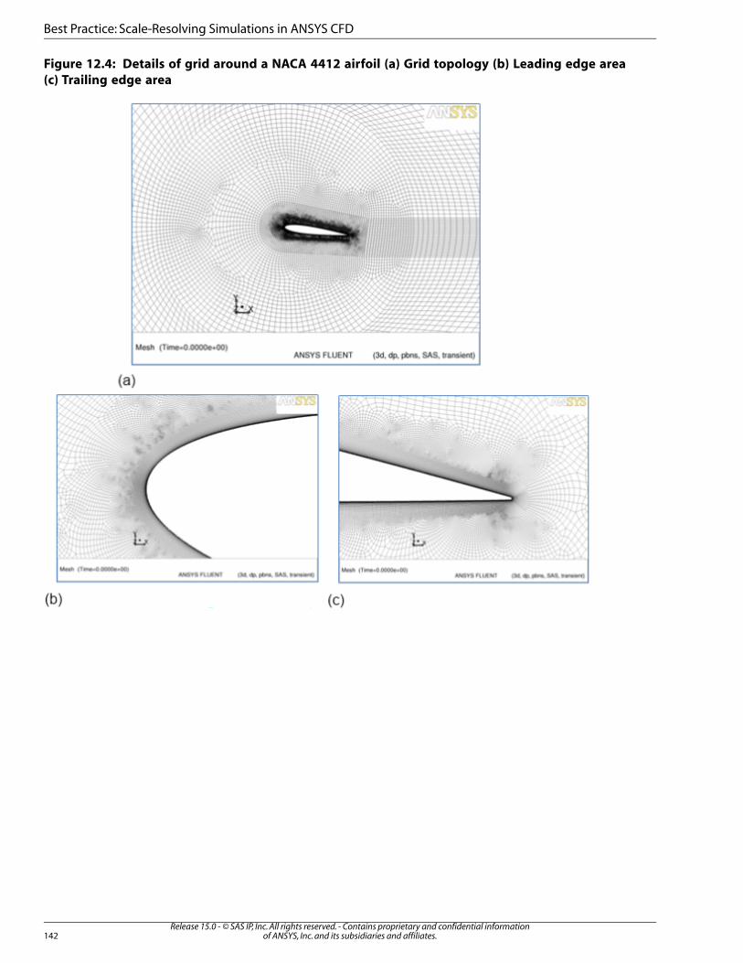
Figure 12.4: Details of grid around a NACA 4412 airfoil (a) Grid topology (b) Leading edge area
(c) Trailing edge area
Release 15.0 - © SAS IP, Inc. All rights reserved. - Contains proprietary and confidential informationof ANSYS, Inc. and its subsidiaries and affiliates.142
Best Practice: Scale-Resolving Simulations in ANSYS CFD
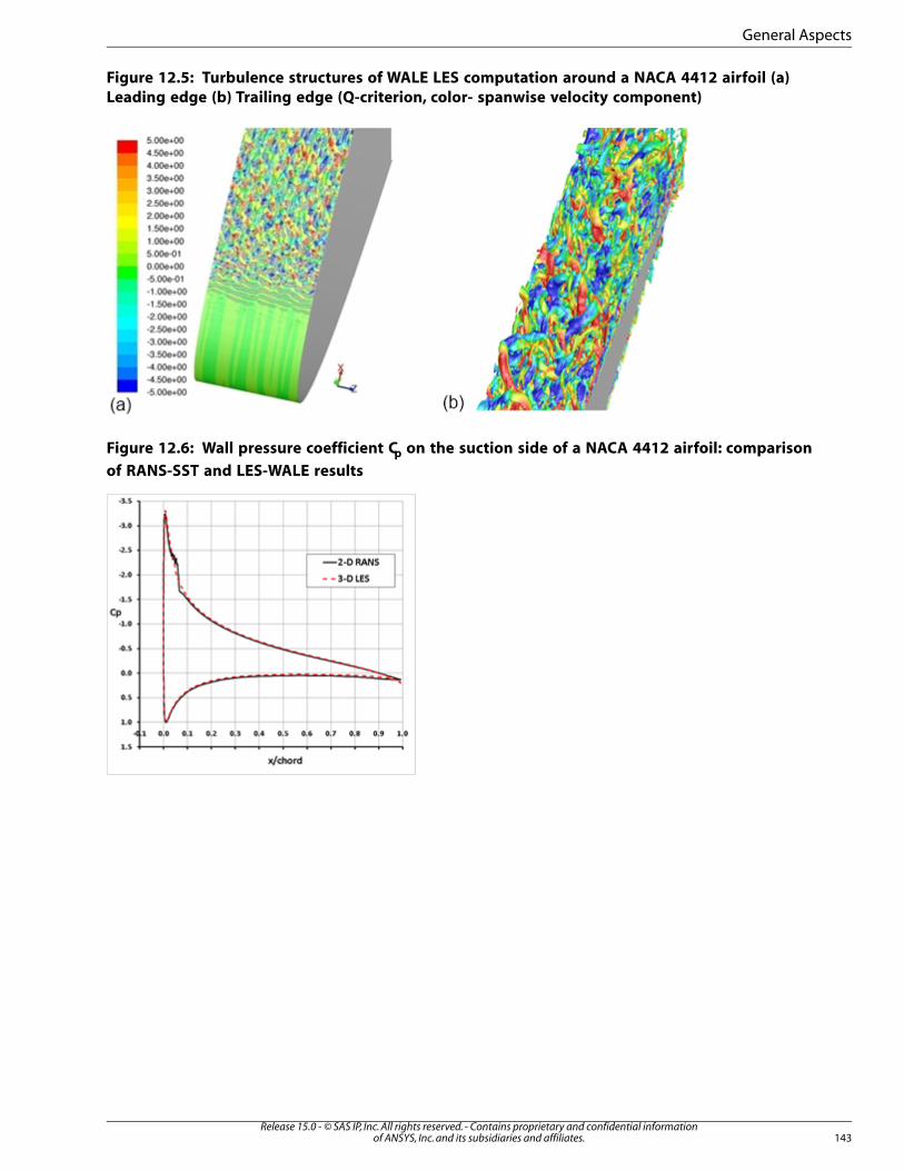
Figure 12.5: Turbulence structures of WALE LES computation around a NACA 4412 airfoil (a)
Leading edge (b) Trailing edge (Q-criterion, color- spanwise velocity component)
Figure 12.6: Wall pressure coefficient Cp on the suction side of a NACA 4412 airfoil: comparison
of RANS-SST and LES-WALE results
143Release 15.0 - © SAS IP, Inc. All rights reserved. - Contains proprietary and confidential information
of ANSYS, Inc. and its subsidiaries and affiliates.
General Aspects

Figure 12.7: Wall shear stress coefficient Cf on the suction side of a NACA 4412 airfoil: comparison
of RANS-SST and LES-WALE results
Overall, LES for industrial flows will be restricted in the foreseeable future to flows not involving wallboundary layers, or wall-bounded flows in strongly reduced geometries, preferentially at low Re numbers.
The limitations of the conventional LES approach are the driving force behind the development of hybridRANS-LES models that are described in the later parts of this report.
12.3. Scale-Resolving Simulation (SRS) Models – Basic Formulations
In the ANSYS CFD codes the following SRS models are available:
1. Scale-Adaptive Simulation (SAS) models
• SAS-SST model (Fluent, CFX)
2. Detached Eddy Simulation (DES) models
• DES-SA (DDES) model (Fluent)
• DES-SST (DDES) model (Fluent, CFX)
• Realizable −� � DES model (Fluent)
3. Large Eddy Simulation (LES)
• Smagorinsky-Lilly model (+dynamic) (Fluent, CFX)
• WALE model (Fluent, CFX)
• Kinetic energy subgrid model dynamic (Fluent)
• Algebraic Wall Modeled LES (WMLES) (Fluent, CFX)
4. Embedded LES (ELES) mode
• Combination of all RANS models with all non-dynamic LES models (Fluent)
Release 15.0 - © SAS IP, Inc. All rights reserved. - Contains proprietary and confidential informationof ANSYS, Inc. and its subsidiaries and affiliates.144
Best Practice: Scale-Resolving Simulations in ANSYS CFD
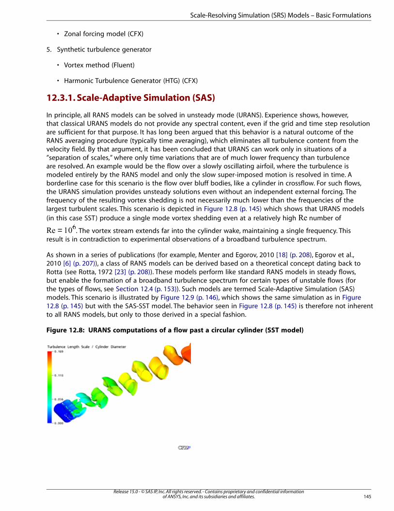
• Zonal forcing model (CFX)
5. Synthetic turbulence generator
• Vortex method (Fluent)
• Harmonic Turbulence Generator (HTG) (CFX)
12.3.1. Scale-Adaptive Simulation (SAS)
In principle, all RANS models can be solved in unsteady mode (URANS). Experience shows, however,that classical URANS models do not provide any spectral content, even if the grid and time step resolutionare sufficient for that purpose. It has long been argued that this behavior is a natural outcome of theRANS averaging procedure (typically time averaging), which eliminates all turbulence content from thevelocity field. By that argument, it has been concluded that URANS can work only in situations of a”separation of scales,” where only time variations that are of much lower frequency than turbulenceare resolved. An example would be the flow over a slowly oscillating airfoil, where the turbulence ismodeled entirely by the RANS model and only the slow super-imposed motion is resolved in time. Aborderline case for this scenario is the flow over bluff bodies, like a cylinder in crossflow. For such flows,the URANS simulation provides unsteady solutions even without an independent external forcing. Thefrequency of the resulting vortex shedding is not necessarily much lower than the frequencies of thelargest turbulent scales. This scenario is depicted in Figure 12.8 (p. 145) which shows that URANS models(in this case SST) produce a single mode vortex shedding even at a relatively high number of
= �. The vortex stream extends far into the cylinder wake, maintaining a single frequency. This
result is in contradiction to experimental observations of a broadband turbulence spectrum.
As shown in a series of publications (for example, Menter and Egorov, 2010 [18] (p. 208), Egorov et al.,2010 [6] (p. 207)), a class of RANS models can be derived based on a theoretical concept dating back toRotta (see Rotta, 1972 [23] (p. 208)). These models perform like standard RANS models in steady flows,but enable the formation of a broadband turbulence spectrum for certain types of unstable flows (forthe types of flows, see Section 12.4 (p. 153)). Such models are termed Scale-Adaptive Simulation (SAS)models. This scenario is illustrated by Figure 12.9 (p. 146), which shows the same simulation as in Figure12.8 (p. 145) but with the SAS-SST model. The behavior seen in Figure 12.8 (p. 145) is therefore not inherentto all RANS models, but only to those derived in a special fashion.
Figure 12.8: URANS computations of a flow past a circular cylinder (SST model)
145Release 15.0 - © SAS IP, Inc. All rights reserved. - Contains proprietary and confidential information
of ANSYS, Inc. and its subsidiaries and affiliates.
Scale-Resolving Simulation (SRS) Models – Basic Formulations

Figure 12.9: SAS simulation of flow past a circular cylinder (SAS-SST model)
The SAS concept is described in much detail in the cited references and will not be repeated here.However, the basic model formulation must be provided for a discussion of the model’s characteristics.The difference between standard RANS and SAS models lies in the treatment of the scale-definingequation (typically �-,�-, or ��-equation). In classic RANS models, the scale equation is modeled based
on an analogy with the �-equation using simple dimensional arguments. The scale equation of SASmodels is based on an exact transport equation for the turbulence length scale as proposed by Rotta.This method was re-visited by Menter and Egorov, 2010 [18] (p. 208) and avoids some limitations of theoriginal Rotta model. As a result of this re-formulation, it was shown that the second derivative of thevelocity field must be included in the source terms of the scale equation. The original SAS model (Menter
and Egorov, 2010 [18] (p. 208)) was formulated as a two-equation model, with the variable =� ���
for the scale equation:
(12.13)∂
∂+
∂∂
= − + ∂∂
∂∂
�
�
� �
�
�
�
�
�� �
�
�
� �
���
�
(12.14)�
∂∂
+∂
∂=
−
− + ∂
∂
∂∂
��
�
�� �
�
!" # #
$
$# �!
%
&
�
'
'(
)
* '
)
+ ', -
-
.
Release 15.0 - © SAS IP, Inc. All rights reserved. - Contains proprietary and confidential informationof ANSYS, Inc. and its subsidiaries and affiliates.146
Best Practice: Scale-Resolving Simulations in ANSYS CFD
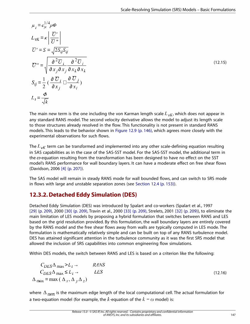
(12.15)
�
=
= ′
′ = =
′′ = ∂∂ ∂
∂∂ ∂
= ∂∂
+∂∂
=
� � ��
� ��
�
� � � �
��
�
��
�
��
� �
�� ��
�
� �
�
� �
���
�
�
�
�
���
� �
The main new term is the one including the von Karman length scale �� �, which does not appear inany standard RANS model. The second velocity derivative allows the model to adjust its length scaleto those structures already resolved in the flow. This functionality is not present in standard RANSmodels. This leads to the behavior shown in Figure 12.9 (p. 146), which agrees more closely with theexperimental observations for such flows.
The �� � term can be transformed and implemented into any other scale-defining equation resultingin SAS capabilities as in the case of the SAS-SST model. For the SAS-SST model, the additional term inthe �-equation resulting from the transformation has been designed to have no effect on the SSTmodel’s RANS performance for wall boundary layers. It can have a moderate effect on free shear flows(Davidson, 2006 [4] (p. 207)).
The SAS model will remain in steady RANS mode for wall bounded flows, and can switch to SRS modein flows with large and unstable separation zones (see Section 12.4 (p. 153)).
12.3.2. Detached Eddy Simulation (DES)
Detached Eddy Simulation (DES) was introduced by Spalart and co-workers (Spalart et al., 1997[29] (p. 209), 2000 [30] (p. 209), Travin et al., 2000 [33] (p. 209), Strelets, 2001 [32] (p. 209)), to eliminate themain limitation of LES models by proposing a hybrid formulation that switches between RANS and LESbased on the grid resolution provided. By this formulation, the wall boundary layers are entirely coveredby the RANS model and the free shear flows away from walls are typically computed in LES mode. Theformulation is mathematically relatively simple and can be built on top of any RANS turbulence model.DES has attained significant attention in the turbulence community as it was the first SRS model thatallowed the inclusion of SRS capabilities into common engineering flow simulations.
Within DES models, the switch between RANS and LES is based on a criterion like the following:
(12.16)
> →≤ →
=
� � �� !
� � �"!
#$% &
#$% &
' ( )
*+,
*+,
*+,
where -./ is the maximum edge length of the local computational cell. The actual formulation for
a two-equation model (for example, the 0-equation of the −1 2 model) is:
147Release 15.0 - © SAS IP, Inc. All rights reserved. - Contains proprietary and confidential information
of ANSYS, Inc. and its subsidiaries and affiliates.
Scale-Resolving Simulation (SRS) Models – Basic Formulations
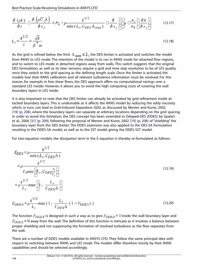
(12.17)∂
∂+
∂∂
= − + ∂∂
+
∂∂
��
�
�� �
�� �
�
� � ��
�
�
�
�
� ��
�
�
���
���
(12.18)= =��
�
�
� ��
���
As the grid is refined below the limit ≤ � !"# the DES-limiter is activated and switches the modelfrom RANS to LES mode. The intention of the model is to run in RANS mode for attached flow regions,and to switch to LES mode in detached regions away from walls. This switch suggests that the originalDES formulation, as well as its later versions, require a grid and time step resolution to be of LES qualityonce they switch to the grid spacing as the defining length scale. Once the limiter is activated, themodels lose their RANS calibration and all relevant turbulence information must be resolved. For thisreason, for example in free shear flows, the DES approach offers no computational savings over astandard LES model. However, it allows you to avoid the high computing costs of covering the wallboundary layers in LES mode.
It is also important to note that the DES limiter can already be activated by grid refinement inside at-tached boundary layers. This is undesirable as it affects the RANS model by reducing the eddy viscositywhich, in turn, can lead to Grid-Induced Separation (GIS), as discussed by Menter and Kuntz, 2002[19] (p. 208), where the boundary layers can separate at arbitrary locations depending on the grid spacing.In order to avoid this limitation, the DES concept has been extended to Delayed-DES (DDES) by Spalartet al., 2006 [31] (p. 209), following the proposal of Menter and Kuntz, 2002 [19] (p. 208) of “shielding” theboundary layer from the DES limiter. The DDES extension was also applied to the DES-SA formulationresulting in the DDES-SA model, as well as to the SST model giving the DDES-SST model.
For two-equation models, the dissipation term in the $-equation is thereby re-formulated as follows:
(12.19)
=
=
=
% &'
( )
&'
( ( )
&'
(
(
)
*+,- *+,
- - *+,.
-
-
*+,
/01
/01
2
/01
3
(12.20)= −4 56
7
7
89::;<
=
=
:;<::;<
>?@
The function ABBCD is designed in such a way as to give =EFFGH inside the wall boundary layer and
=IJJKL away from the wall. The definition of this function is intricate as it involves a balance betweenproper shielding and not suppressing the formation of resolved turbulence as the flow separates fromthe wall.
There are a number of DDES models available in ANSYS CFD. They follow the same principal idea withrespect to switching between RANS and LES mode. The models differ therefore mostly by their RANScapabilities and should be selected accordingly.
Release 15.0 - © SAS IP, Inc. All rights reserved. - Contains proprietary and confidential informationof ANSYS, Inc. and its subsidiaries and affiliates.148
Best Practice: Scale-Resolving Simulations in ANSYS CFD
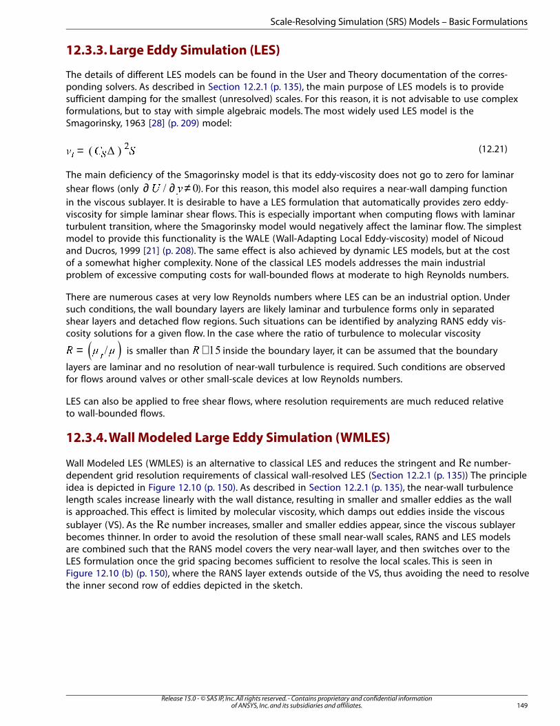
12.3.3. Large Eddy Simulation (LES)
The details of different LES models can be found in the User and Theory documentation of the corres-ponding solvers. As described in Section 12.2.1 (p. 135), the main purpose of LES models is to providesufficient damping for the smallest (unresolved) scales. For this reason, it is not advisable to use complexformulations, but to stay with simple algebraic models. The most widely used LES model is theSmagorinsky, 1963 [28] (p. 209) model:
(12.21)=� � �� ��
The main deficiency of the Smagorinsky model is that its eddy-viscosity does not go to zero for laminar
shear flows (only ∂ ∂ ≠� � ). For this reason, this model also requires a near-wall damping functionin the viscous sublayer. It is desirable to have a LES formulation that automatically provides zero eddy-viscosity for simple laminar shear flows. This is especially important when computing flows with laminarturbulent transition, where the Smagorinsky model would negatively affect the laminar flow. The simplestmodel to provide this functionality is the WALE (Wall-Adapting Local Eddy-viscosity) model of Nicoudand Ducros, 1999 [21] (p. 208). The same effect is also achieved by dynamic LES models, but at the costof a somewhat higher complexity. None of the classical LES models addresses the main industrialproblem of excessive computing costs for wall-bounded flows at moderate to high Reynolds numbers.
There are numerous cases at very low Reynolds numbers where LES can be an industrial option. Undersuch conditions, the wall boundary layers are likely laminar and turbulence forms only in separatedshear layers and detached flow regions. Such situations can be identified by analyzing RANS eddy vis-cosity solutions for a given flow. In the case where the ratio of turbulence to molecular viscosity
=�
is smaller than ∼� inside the boundary layer, it can be assumed that the boundary
layers are laminar and no resolution of near-wall turbulence is required. Such conditions are observedfor flows around valves or other small-scale devices at low Reynolds numbers.
LES can also be applied to free shear flows, where resolution requirements are much reduced relativeto wall-bounded flows.
12.3.4. Wall Modeled Large Eddy Simulation (WMLES)
Wall Modeled LES (WMLES) is an alternative to classical LES and reduces the stringent and number-dependent grid resolution requirements of classical wall-resolved LES (Section 12.2.1 (p. 135)) The principleidea is depicted in Figure 12.10 (p. 150). As described in Section 12.2.1 (p. 135), the near-wall turbulencelength scales increase linearly with the wall distance, resulting in smaller and smaller eddies as the wallis approached. This effect is limited by molecular viscosity, which damps out eddies inside the viscoussublayer (VS). As the number increases, smaller and smaller eddies appear, since the viscous sublayerbecomes thinner. In order to avoid the resolution of these small near-wall scales, RANS and LES modelsare combined such that the RANS model covers the very near-wall layer, and then switches over to theLES formulation once the grid spacing becomes sufficient to resolve the local scales. This is seen inFigure 12.10 (b) (p. 150), where the RANS layer extends outside of the VS, thus avoiding the need to resolvethe inner second row of eddies depicted in the sketch.
149Release 15.0 - © SAS IP, Inc. All rights reserved. - Contains proprietary and confidential information
of ANSYS, Inc. and its subsidiaries and affiliates.
Scale-Resolving Simulation (SRS) Models – Basic Formulations
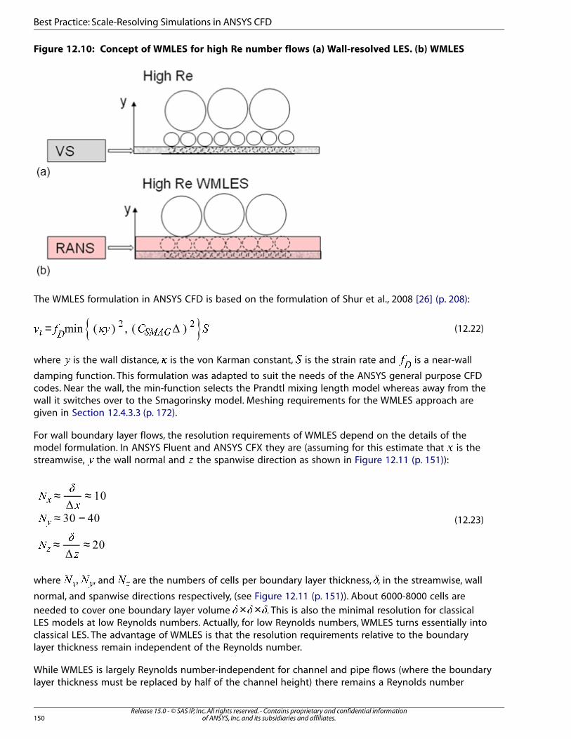
Figure 12.10: Concept of WMLES for high Re number flows (a) Wall-resolved LES. (b) WMLES
The WMLES formulation in ANSYS CFD is based on the formulation of Shur et al., 2008 [26] (p. 208):
(12.22)=� � �� � �� � ��� �
where is the wall distance, � is the von Karman constant, � is the strain rate and ��
is a near-wall
damping function. This formulation was adapted to suit the needs of the ANSYS general purpose CFDcodes. Near the wall, the min-function selects the Prandtl mixing length model whereas away from thewall it switches over to the Smagorinsky model. Meshing requirements for the WMLES approach aregiven in Section 12.4.3.3 (p. 172).
For wall boundary layer flows, the resolution requirements of WMLES depend on the details of themodel formulation. In ANSYS Fluent and ANSYS CFX they are (assuming for this estimate that � is thestreamwise, � the wall normal and � the spanwise direction as shown in Figure 12.11 (p. 151)):
(12.23)
≈ ≈
≈ −
≈ ≈
��
�
�
��
�
�
�
�
where ��,��, and ! are the numbers of cells per boundary layer thickness, ", in the streamwise, wall
normal, and spanwise directions respectively, (see Figure 12.11 (p. 151)). About 6000-8000 cells are
needed to cover one boundary layer volume × ×# # #. This is also the minimal resolution for classicalLES models at low Reynolds numbers. Actually, for low Reynolds numbers, WMLES turns essentially intoclassical LES. The advantage of WMLES is that the resolution requirements relative to the boundarylayer thickness remain independent of the Reynolds number.
While WMLES is largely Reynolds number-independent for channel and pipe flows (where the boundarylayer thickness must be replaced by half of the channel height) there remains a Reynolds number
Release 15.0 - © SAS IP, Inc. All rights reserved. - Contains proprietary and confidential informationof ANSYS, Inc. and its subsidiaries and affiliates.150
Best Practice: Scale-Resolving Simulations in ANSYS CFD
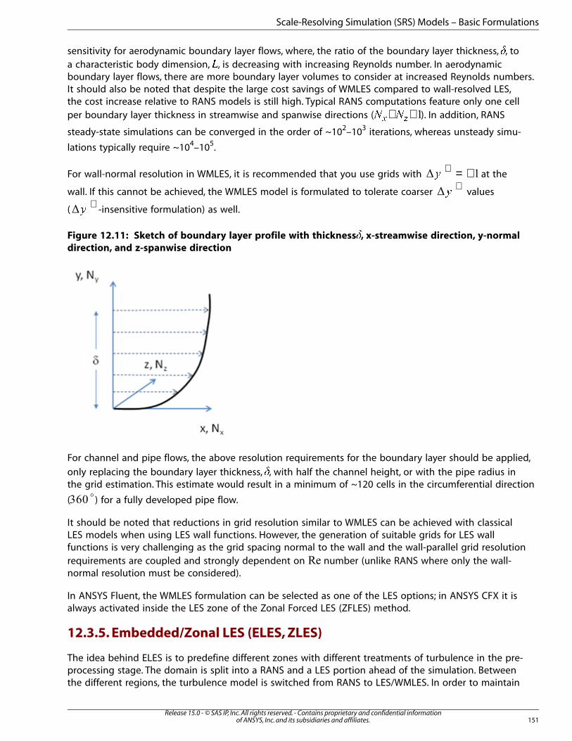
sensitivity for aerodynamic boundary layer flows, where, the ratio of the boundary layer thickness, �, toa characteristic body dimension,�, is decreasing with increasing Reynolds number. In aerodynamicboundary layer flows, there are more boundary layer volumes to consider at increased Reynolds numbers.It should also be noted that despite the large cost savings of WMLES compared to wall-resolved LES,the cost increase relative to RANS models is still high. Typical RANS computations feature only one cellper boundary layer thickness in streamwise and spanwise directions ( ∼ ∼� �� � ). In addition, RANS
steady-state simulations can be converged in the order of ~102–103 iterations, whereas unsteady simu-
lations typically require ~104–105.
For wall-normal resolution in WMLES, it is recommended that you use grids with = ∼+� at the
wall. If this cannot be achieved, the WMLES model is formulated to tolerate coarser +
� values
(+
� -insensitive formulation) as well.
Figure 12.11: Sketch of boundary layer profile with thickness �, x-streamwise direction, y-normal
direction, and z-spanwise direction
For channel and pipe flows, the above resolution requirements for the boundary layer should be applied,
only replacing the boundary layer thickness, , with half the channel height, or with the pipe radius inthe grid estimation. This estimate would result in a minimum of ~120 cells in the circumferential direction
(o
) for a fully developed pipe flow.
It should be noted that reductions in grid resolution similar to WMLES can be achieved with classicalLES models when using LES wall functions. However, the generation of suitable grids for LES wallfunctions is very challenging as the grid spacing normal to the wall and the wall-parallel grid resolutionrequirements are coupled and strongly dependent on number (unlike RANS where only the wall-normal resolution must be considered).
In ANSYS Fluent, the WMLES formulation can be selected as one of the LES options; in ANSYS CFX it isalways activated inside the LES zone of the Zonal Forced LES (ZFLES) method.
12.3.5. Embedded/Zonal LES (ELES, ZLES)
The idea behind ELES is to predefine different zones with different treatments of turbulence in the pre-processing stage. The domain is split into a RANS and a LES portion ahead of the simulation. Betweenthe different regions, the turbulence model is switched from RANS to LES/WMLES. In order to maintain
151Release 15.0 - © SAS IP, Inc. All rights reserved. - Contains proprietary and confidential information
of ANSYS, Inc. and its subsidiaries and affiliates.
Scale-Resolving Simulation (SRS) Models – Basic Formulations

consistency, synthetic turbulence is generally introduced at RANS-LES interfaces. ELES is actually not anew model, but an infrastructure that combines existing elements of technology in a zonal fashion. Therecommendations for each zone are therefore the same as those applicable to the individual models.
In ANSYS Fluent, an Embedded LES formulation is available (Cokljat et al., 2009 [2] (p. 207)). It allows thecombination of most RANS models with all non-dynamic LES models in the predefined RANS and LESregions respectively. The conversion from modeled turbulence to resolved turbulence is achieved atthe RANS-LES interface using the Vortex Method (Mathey et al., 2003 [15] (p. 208)).
In CFX, a similar functionality is achieved using a method called Zonal Forced LES (ZFLES) (Menter etal., 2009 [17] (p. 208)). The simulation is based on a pre-selected RANS model. In a LES zone, specifiedvia a CEL expression, forcing terms in the momentum and turbulence equations are activated. Theseterms push the RANS model into a WMLES formulation. In addition, synthetic turbulence is generatedat the RANS-LES interface,
An additional option in ANSYS Fluent involves using a global turbulence model (SAS or DDES), and ac-tivates the generation of synthetic turbulence at a pre-defined interface. The code takes care of balancingthe resolved and modeled turbulence through the interface. This option can be used to force globalhybrid models (like SAS or DDES) into unsteadiness for cases where the natural flow instability is notsufficient. Unlike ELES, the same turbulence model is used upstream and downstream of the interface.In ELES, different models are used in different zones on opposite sides of the interface.
Such forcing can also by achieved in ANSYS CFX by specifying a thin LES region and using the SAS orDDES model globally.
12.3.6. Unsteady Inlet/Interface Turbulence
Classical LES requires providing unsteady fluctuations at turbulent inlets/interfaces (RANS-LES interface)to the LES domain. This makes LES substantially more demanding than RANS, where profiles of the
mean turbulence quantities (� and � or � and �) are typically specified. An example is a fully turbulentchannel (pipe) flow. The flow enters the domain in a fully turbulent state at the inlet, so you are thereforerequired to provide suitable resolved turbulence at such an inlet location through unsteady inlet velocityprofiles. The inlet profiles have to be composed in such a way that their time average corresponds tothe correct mean flow inlet profiles, as well as to all relevant turbulence characteristics (turbulence timeand length scales, turbulence stresses, and so on). For fully turbulent channel and pipe flows, this re-quirement can be circumvented by the application of periodic boundary conditions in the flow direction.The flow is thereby driven by a source term in the momentum equation acting in the streamwise direc-tion. By that trick, the turbulence leaving the domain at the outlet enters the domain again at the inlet,thereby avoiding the explicit specification of unsteady turbulence profiles. This approach can be employedfor only very simple configurations. It requires a sufficient length of the domain (at least ~8–10h, seeFigure 12.3 (p. 139)) in the streamwise direction to enable the formation inside the domain of turbulencestructures independent of the periodic boundaries.
In most practical cases, the geometry does not enable fully periodic simulations. It can however featurefully developed profiles at the inlet (again typically pipe/channel flows). In such cases, you can performa periodic precursor simulation on a separate periodic domain and then insert the unsteady profilesobtained at any cross section of that simulation to the inlet of the complex CFD domain. This approachrequires either a direct coupling of two separate CFD simulations or the storage of a sufficient numberof unsteady profiles from the periodic simulation to be read in by the full simulation.
In a real situation, however, the inlet profiles might not be fully developed and no simple method existsfor producing consistent inlet turbulence. In such cases, synthetic turbulence can be generated, based
Release 15.0 - © SAS IP, Inc. All rights reserved. - Contains proprietary and confidential informationof ANSYS, Inc. and its subsidiaries and affiliates.152
Best Practice: Scale-Resolving Simulations in ANSYS CFD
on given inlet profiles from RANS. These are typically obtained from a precursor RANS computation ofthe domain upstream of the LES inlet.
There are several methods for generating synthetic turbulence. In ANSYS Fluent, the most widely usedmethod is the Vortex Method (VM) (see Mathey et al., 2003 [15] (p. 208)), where a number of discretevortices are generated at the inlet. Their distribution, strength, and size are modeled to provide thedesirable characteristics of real turbulence. The input parameters to the VM are the two scales (k and� or k and �) from the upstream RANS computation. CFX uses the generation of synthetic turbulenceby using suitable harmonic functions as an alternative to the VM (e.g. Menter et al., 2009 [17] (p. 208)).
The characteristic of high-quality synthetic turbulence in wall-bounded flows is that it recovers the time-averaged turbulent stress tensor quickly downstream of the inlet. This can be checked by plottingsensitive quantities like the time-averaged wall shear stress or heat transfer coefficient and observingtheir variation downstream of the inlet. It is also advisable to investigate the turbulence structures
visually by using, for example, an iso-surface of the �-criterion, = −� � �� �
(where � is the
Strain rate, and � is the vorticity rate). This can be done even after a few hundred time steps into thesimulation.
Because synthetic turbulence will never coincide in all aspects with true turbulence, avoid putting aninlet/interface at a location with strong non-equilibrium turbulence activity. In boundary layer flows,that means that the inlet or RANS-LES interface should be located several (at least ∼ 3) boundary layerthicknesses upstream of any strong non-equilibrium zone (such as a separation). The boundary layersdownstream of the inlet/interface need to be resolved with a sufficiently high spatial resolution (seeSection 12.4.3.3 (p. 172)).
12.4. Generic Flow Types and Basic Model Selection
As will be discussed, there is a wide range of complex industrial turbulent flows and there is no singleSRS approach to cover all of them with high efficiency. The most difficult question as you use the softwareis therefore how to select the optimal model combination for a given simulation. For this task, it isuseful to categorize flows into different types. Although such a categorization is not always easy andby no means scientifically exact (there are many flows that do not exactly fall into any one of the pro-posed categories or fall into more than one) it might still help in the selection of the most appropriateSRS modeling approach.
12.4.1. Globally Unstable Flows
12.4.1.1. Flow Physics
The classical example of a globally unstable flow is a flow past a bluff body. Even when computed witha classical URANS model, the simulation will typically provide an unsteady output. Figure 12.14 (p. 158)shows the flow around a triangular cylinder in crossflow as computed with both the SAS-SST and theDES-SST model. It is important to emphasize that the flow is computed with steady-state boundaryconditions (as would be employed for a RANS simulation). Still, the flow downstream of the obstacleturns quickly into unsteady (scale-resolving) mode, even though no unsteadiness is introduced by anyboundary or interface condition.
From a physical standpoint, such flows are characterized by the formation of new turbulence downstreamof the body. This turbulence is independent from, and effectively overrides, the turbulence coming fromthe thin, attached boundary layers around the body. The turbulence in the attached boundary layershas very little effect on the turbulence in the separated zone. The attached boundary layers can, however,
153Release 15.0 - © SAS IP, Inc. All rights reserved. - Contains proprietary and confidential information
of ANSYS, Inc. and its subsidiaries and affiliates.
Generic Flow Types and Basic Model Selection
define the separation point/line on a smoothly curved body and so affect the size of the downstreamseparation zone. This effect can be tackled by a suitable underlying RANS model.
Typical members of this family of flows are given in the list below. Such flows are very common in en-gineering applications and are also the type of flows where RANS models can exhibit a significant de-terioration of their predictive accuracy.
Examples of globally unstable flows include:
• Flows past bluff bodies include:
– Flow past buildings
– Landing gears of airplanes
– Baffles in mixers
– Side mirrors of cars
– Stalled wings/sails
– Re-entry vehicles
– Trains/trucks/cars in crossflow
– Tip gap of turbomachinery blades
– Flows past orifices, sharp nozzles
– Cavities
– Flows with large separation zones (relative to attached boundary layer thickness)
• Flows with strong swirl instabilities include:
– Flow in combustion chambers of gas turbines
– Flows past vortex generators
– Some tip vortex flows in adverse pressure gradients
• Flows with strong flow interaction include:
– Impinging/colliding jets
– Jets in crossflow
The color scheme of the preceding points above identifies flows that are clearly within the definitionof globally unstable flows (black) and those where the type of the flow depends on details of its re-gime/geometry (gray). Such flows fall in-between globally and locally unstable flows (see Sec-tion 12.4.2 (p. 164)).
12.4.1.2. Modeling
Of all flows where SRS modeling is required, globally unstable flows are conceptually the easiest tohandle. They can be typically captured by a global RANS-LES model such as SAS or DDES. Such models
Release 15.0 - © SAS IP, Inc. All rights reserved. - Contains proprietary and confidential informationof ANSYS, Inc. and its subsidiaries and affiliates.154
Best Practice: Scale-Resolving Simulations in ANSYS CFD
cover the attached and mildly separated boundary layers in RANS mode, thereby avoiding the highcosts of resolving wall turbulence. Due to the strong flow instability past the separation line, there isno need for specifying unsteady inlet turbulence nor to define specific LES zones. Globally unstableflows are also the most beneficial for SRS, as experience shows that RANS models can fail with significantmargins of error for such flows. A large number of industrial flows fall into this category.
The safest SRS model for such flows is the SAS approach. It offers the advantage that the RANS modelis not affected by the grid spacing and thereby avoids the potential negative effects of (D)DES (grayzones or grid induced separation). The SAS concept reverts back to (U)RANS in case the mesh/time stepis not sufficient for LES and thereby preserves a backbone of modeling that is independent of spaceand time resolution, though at the increased cost that is associated with any transient SRS calculation.SAS also avoids the need for shielding, which for internal flows with multiple walls can suppress turbu-lence formation in DDES models.
The alternative to SAS is DDES. If proper care is taken to ensure LES mesh quality in the detached flowregions, the model will be operating in the environment for which it was designed, typically providinghigh-quality solutions. DDES has shown advantages for flows at the limit of globally unstable flows (seeFigure 12.43 (p. 187)) where the SAS model can produce URANS-like solutions. In cases like these, DDESstill provides SRS in the separated regions.
For globally unstable flows, the behavior of SAS and DDES is often very similar and they should bothbe tried.
12.4.1.3. Meshing Requirements
The part of the domain where the turbulence model acts in RANS mode has to be covered by a suitableRANS grid. It is especially important that all relevant boundary layers are covered with sufficient resolution(typically a minimum of 10–15 structured cells across the boundary layer). It is assumed that you arefamiliar with grid requirements for RANS simulations.
The estimate for the lowest possible mesh resolution in the detached SRS region is based on the as-sumption that the largest relevant scales are similar in size to the width of the instability zone. For abluff body, the width is the diameter D of the body; for a combustor, the width is the diameter of thecore vortex; for a jet in crossflow, the width is the diameter of the jet; and so on. Experience shows thatthe minimum resolution for such flows is of the order:
(12.24)≤ ����
This resolution requires more than 20 cells per characteristic diameter,� (in some applications withvery strong instabilities, even 10 cells across the layer may be sufficient). As is generally the case forSRS, it is best to provide isotropic (cubic) cells, or at least to avoid large aspect ratios (aspect ratiossmaller than 5 would be optimal, but cannot always be achieved in complex geometries).
With the above estimate for ���, there is a good chance of resolving the main flow instability andthe resulting strong turbulent mixing processes associated with the global flow instability (an effectoften missed by RANS models). For acoustics simulations, it might also be important to resolve theturbulence generated in the (often thin) shear layer that is separating from the body. Resolving thisturbulence poses a much more stringent demand on grid resolution on the simulation, as the shearlayer scales with the boundary layer thickness at separation and so can be much smaller than the bodydimension. This situation is covered in Section 12.4.2 (p. 164).
155Release 15.0 - © SAS IP, Inc. All rights reserved. - Contains proprietary and confidential information
of ANSYS, Inc. and its subsidiaries and affiliates.
Generic Flow Types and Basic Model Selection
12.4.1.4. Numerical Settings
The general numerical settings are described in Section 12.5 (p. 192). Globally unstable flows are relativelyforgiving with respect to numerics, at least as far as the mean flow characteristics are concerned. Therecommended choice for the advection terms is the Bounded Central Difference (BCD) scheme, especiallyfor complex geometries and flows. For such flows, the classical Central Difference (CD) scheme can beunstable or produce unphysical wiggles in the solution (see Figure 12.51 (p. 193)). The BCD scheme isslightly more dissipative, but is substantially more robust and is therefore frequently the optimal choice.If a visual inspection of the flow (see Section 12.7.1 (p. 197)) shows that turbulence structures are notproduced in agreement with the expectations for the flow, you can switch to CD. If this switch is made,it is advisable to closely monitor the solution (visually and numerically through residuals) to ensure thatwiggles are not dominating the simulation. With SAS the “Least Square Cell Based” or the “Node-BasedGreen Gauss” gradient method should be used in ANSYS Fluent. The latter allows a slightly better rep-resentation of the second derivative of the velocity field that is required for the model formulation (vonKarman length scale).
In ANSYS CFX, the default hybrid numerical option switches explicitly between the High ResolutionScheme (in the RANS region) and the CD scheme (in the LES region). For most applications, it appearsthat the use of the BCD scheme should also be favored in ANSYS CFX (see also Section 12.5.1.1 (p. 192))
12.4.1.5. Examples
12.4.1.5.1. Flow around a Fighter Aircraft
Figure 12.12 (p. 157) shows a highly complex, globally unstable flow field, around a generic fighter aircraftgeometry at high angle of attack as computed with the SAS-SST model. The grid consists of 108 hybridcells. This simulation is currently in progress within the EU project ATAAC and no detailed discussionof this flow is intended. Figure 12.12 (p. 157) demonstrates the complex regional appearance of resolvedturbulence around the aircraft. It is obvious that the application of global models like SAS or DDESgreatly simplifies the setup for such flows compared to using ELES/ZLES, where you would have todefine the LES regions and suitable interfaces between the RANS and LES regions in a pre-processingstep. In contracts, when using global models, the simulation is first carried out in standard RANS mode.Starting from that RANS solution, the model is then simply switched to the SAS or DDES variant of theRANS model, the solver is set to unsteady mode, and the numeric is adjusted according to Sec-tion 12.4.1.4 (p. 156). No further adjustment is required in order to produce the solutions shown in Figure12.12 (p. 157).
Release 15.0 - © SAS IP, Inc. All rights reserved. - Contains proprietary and confidential informationof ANSYS, Inc. and its subsidiaries and affiliates.156
Best Practice: Scale-Resolving Simulations in ANSYS CFD
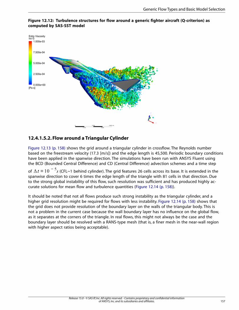
Figure 12.12: Turbulence structures for flow around a generic fighter aircraft (Q-criterion) as
computed by SAS-SST model
12.4.1.5.2. Flow around a Triangular Cylinder
Figure 12.13 (p. 158) shows the grid around a triangular cylinder in crossflow. The Reynolds numberbased on the freestream velocity (17.3 [m/s]) and the edge length is 45,500. Periodic boundary conditionshave been applied in the spanwise direction. The simulations have been run with ANSYS Fluent usingthe BCD (Bounded Central Difference) and CD (Central Difference) advection schemes and a time step
of = −� �
� (CFL~1 behind cylinder). The grid features 26 cells across its base. It is extended in the
spanwise direction to cover 6 times the edge length of the triangle with 81 cells in that direction. Dueto the strong global instability of this flow, such resolution was sufficient and has produced highly ac-curate solutions for mean flow and turbulence quantities (Figure 12.14 (p. 158)).
It should be noted that not all flows produce such strong instability as the triangular cylinder, and ahigher grid resolution might be required for flows with less instability. Figure 12.14 (p. 158) shows thatthe grid does not provide resolution of the boundary layer on the walls of the triangular body. This isnot a problem in the current case because the wall boundary layer has no influence on the global flow,as it separates at the corners of the triangle. In real flows, this might not always be the case and theboundary layer should be resolved with a RANS-type mesh (that is, a finer mesh in the near-wall regionwith higher aspect ratios being acceptable).
157Release 15.0 - © SAS IP, Inc. All rights reserved. - Contains proprietary and confidential information
of ANSYS, Inc. and its subsidiaries and affiliates.
Generic Flow Types and Basic Model Selection
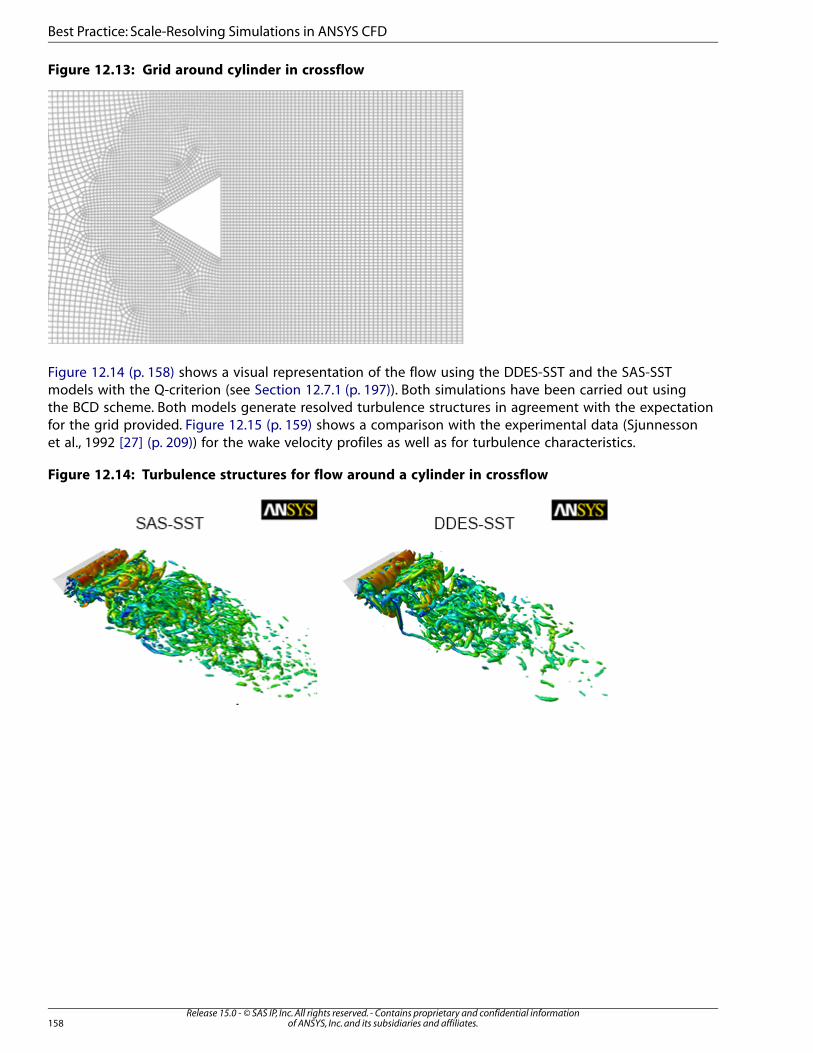
Figure 12.13: Grid around cylinder in crossflow
Figure 12.14 (p. 158) shows a visual representation of the flow using the DDES-SST and the SAS-SSTmodels with the Q-criterion (see Section 12.7.1 (p. 197)). Both simulations have been carried out usingthe BCD scheme. Both models generate resolved turbulence structures in agreement with the expectationfor the grid provided. Figure 12.15 (p. 159) shows a comparison with the experimental data (Sjunnessonet al., 1992 [27] (p. 209)) for the wake velocity profiles as well as for turbulence characteristics.
Figure 12.14: Turbulence structures for flow around a cylinder in crossflow
Release 15.0 - © SAS IP, Inc. All rights reserved. - Contains proprietary and confidential informationof ANSYS, Inc. and its subsidiaries and affiliates.158
Best Practice: Scale-Resolving Simulations in ANSYS CFD
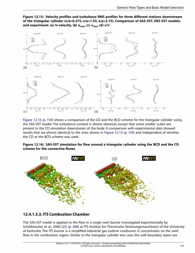
Figure 12.15: Velocity profiles and turbulence RMS profiles for three different stations downstream
of the triangular cylinder (x/a=0.375, x/a=1.53, x/a=3.75). Comparison of SAS-SST, DES-SST models,
and experiment. (a) U-velocity, (b) urms, (c) vrms, (d) u’v’
Figure 12.16 (p. 159) shows a comparison of the CD and the BCD scheme for the triangular cylinder usingthe SAS-SST model. The turbulence content is almost identical, except that some smaller scales arepresent in the CD simulation downstream of the body. A comparison with experimental data showedresults that are almost identical to the ones shown in Figure 12.15 (p. 159) and independent of whetherthe CD or the BCD scheme was used.
Figure 12.16: SAS-SST simulation for flow around a triangular cylinder using the BCD and the CD
scheme for the convective fluxes
12.4.1.5.3. ITS Combustion Chamber
The SAS-SST model is applied to the flow in a single swirl burner investigated experimentally bySchildmacher et al., 2000 [25] (p. 208) at ITS (Institut für Thermische Strömungsmaschinen) of the Universityof Karlsruhe. The ITS burner is a simplified industrial gas turbine combustor. It concentrates on the swirlflow in the combustion region. Similar to the triangular cylinder test case, the wall boundary layers are
159Release 15.0 - © SAS IP, Inc. All rights reserved. - Contains proprietary and confidential information
of ANSYS, Inc. and its subsidiaries and affiliates.
Generic Flow Types and Basic Model Selection
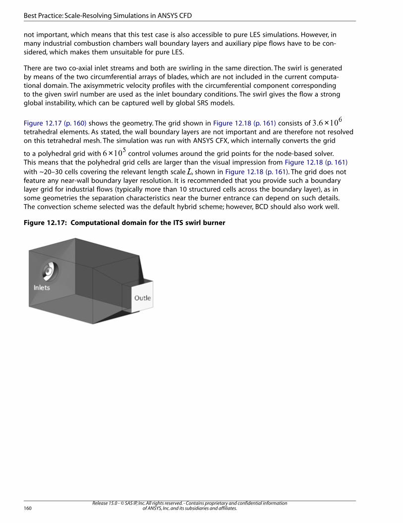
not important, which means that this test case is also accessible to pure LES simulations. However, inmany industrial combustion chambers wall boundary layers and auxiliary pipe flows have to be con-sidered, which makes them unsuitable for pure LES.
There are two co-axial inlet streams and both are swirling in the same direction. The swirl is generatedby means of the two circumferential arrays of blades, which are not included in the current computa-tional domain. The axisymmetric velocity profiles with the circumferential component correspondingto the given swirl number are used as the inlet boundary conditions. The swirl gives the flow a strongglobal instability, which can be captured well by global SRS models.
Figure 12.17 (p. 160) shows the geometry. The grid shown in Figure 12.18 (p. 161) consists of × �
tetrahedral elements. As stated, the wall boundary layers are not important and are therefore not resolvedon this tetrahedral mesh. The simulation was run with ANSYS CFX, which internally converts the grid
to a polyhedral grid with × � control volumes around the grid points for the node-based solver.
This means that the polyhedral grid cells are larger than the visual impression from Figure 12.18 (p. 161)with ~20–30 cells covering the relevant length scale �, shown in Figure 12.18 (p. 161). The grid does notfeature any near-wall boundary layer resolution. It is recommended that you provide such a boundarylayer grid for industrial flows (typically more than 10 structured cells across the boundary layer), as insome geometries the separation characteristics near the burner entrance can depend on such details.The convection scheme selected was the default hybrid scheme; however, BCD should also work well.
Figure 12.17: Computational domain for the ITS swirl burner
Release 15.0 - © SAS IP, Inc. All rights reserved. - Contains proprietary and confidential informationof ANSYS, Inc. and its subsidiaries and affiliates.160
Best Practice: Scale-Resolving Simulations in ANSYS CFD
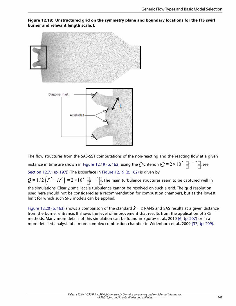
Figure 12.18: Unstructured grid on the symmetry plane and boundary locations for the ITS swirl
burner and relevant length scale, L
The flow structures from the SAS-SST computations of the non-reacting and the reacting flow at a given
instance in time are shown in Figure 12.19 (p. 162) using the �-criterion ( = ×
−� �
� �, see
Section 12.7.1 (p. 197)). The isosurface in Figure 12.19 (p. 162) is given by
= − = ×
−� � � �
. The main turbulence structures seem to be captured well in
the simulations. Clearly, small-scale turbulence cannot be resolved on such a grid. The grid resolutionused here should not be considered as a recommendation for combustion chambers, but as the lowestlimit for which such SRS models can be applied.
Figure 12.20 (p. 163) shows a comparison of the standard −� � RANS and SAS results at a given distancefrom the burner entrance. It shows the level of improvement that results from the application of SRSmethods. Many more details of this simulation can be found in Egorov et al., 2010 [6] (p. 207) or in amore detailed analysis of a more complex combustion chamber in Widenhorn et al., 2009 [37] (p. 209).
161Release 15.0 - © SAS IP, Inc. All rights reserved. - Contains proprietary and confidential information
of ANSYS, Inc. and its subsidiaries and affiliates.
Generic Flow Types and Basic Model Selection
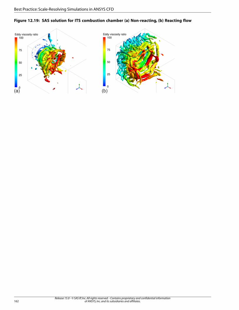
Figure 12.19: SAS solution for ITS combustion chamber (a) Non-reacting, (b) Reacting flow
Release 15.0 - © SAS IP, Inc. All rights reserved. - Contains proprietary and confidential informationof ANSYS, Inc. and its subsidiaries and affiliates.162
Best Practice: Scale-Resolving Simulations in ANSYS CFD
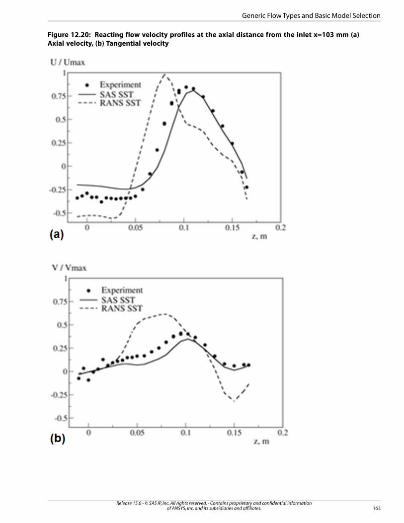
Figure 12.20: Reacting flow velocity profiles at the axial distance from the inlet x=103 mm (a)
Axial velocity, (b) Tangential velocity
163Release 15.0 - © SAS IP, Inc. All rights reserved. - Contains proprietary and confidential information
of ANSYS, Inc. and its subsidiaries and affiliates.
Generic Flow Types and Basic Model Selection
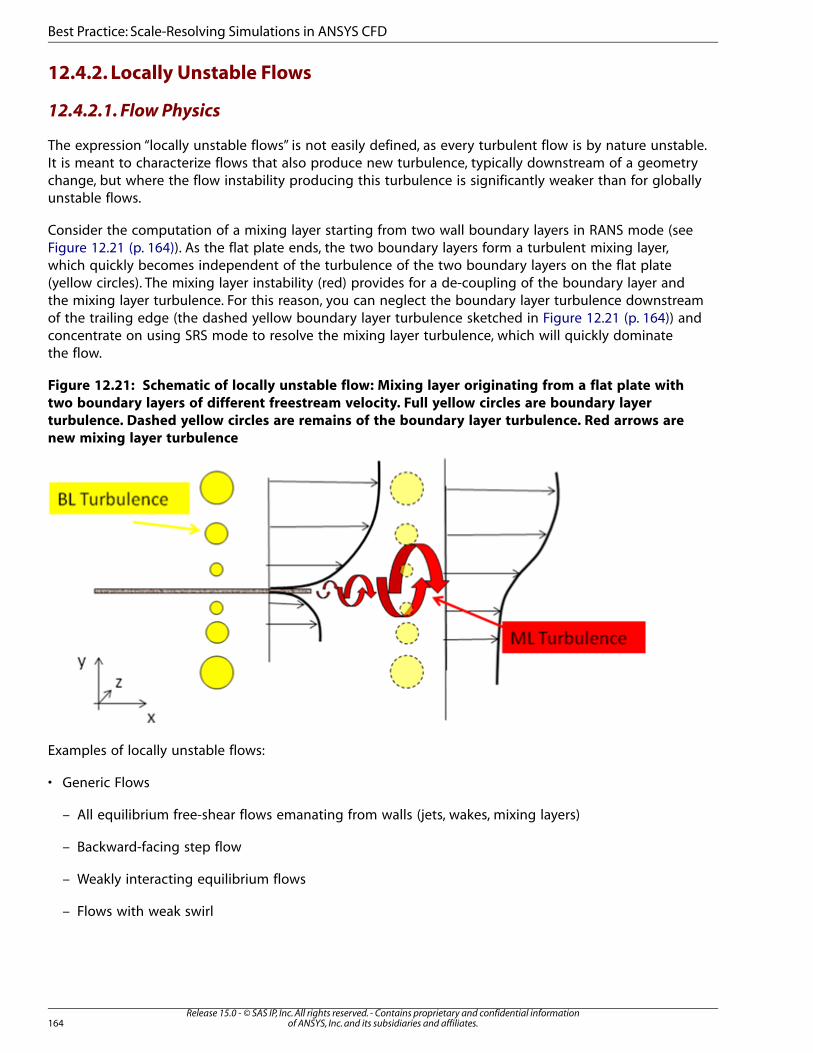
12.4.2. Locally Unstable Flows
12.4.2.1. Flow Physics
The expression “locally unstable flows” is not easily defined, as every turbulent flow is by nature unstable.It is meant to characterize flows that also produce new turbulence, typically downstream of a geometrychange, but where the flow instability producing this turbulence is significantly weaker than for globallyunstable flows.
Consider the computation of a mixing layer starting from two wall boundary layers in RANS mode (seeFigure 12.21 (p. 164)). As the flat plate ends, the two boundary layers form a turbulent mixing layer,which quickly becomes independent of the turbulence of the two boundary layers on the flat plate(yellow circles). The mixing layer instability (red) provides for a de-coupling of the boundary layer andthe mixing layer turbulence. For this reason, you can neglect the boundary layer turbulence downstreamof the trailing edge (the dashed yellow boundary layer turbulence sketched in Figure 12.21 (p. 164)) andconcentrate on using SRS mode to resolve the mixing layer turbulence, which will quickly dominatethe flow.
Figure 12.21: Schematic of locally unstable flow: Mixing layer originating from a flat plate with
two boundary layers of different freestream velocity. Full yellow circles are boundary layer
turbulence. Dashed yellow circles are remains of the boundary layer turbulence. Red arrows are
new mixing layer turbulence
Examples of locally unstable flows:
• Generic Flows
– All equilibrium free-shear flows emanating from walls (jets, wakes, mixing layers)
– Backward-facing step flow
– Weakly interacting equilibrium flows
– Flows with weak swirl
Release 15.0 - © SAS IP, Inc. All rights reserved. - Contains proprietary and confidential informationof ANSYS, Inc. and its subsidiaries and affiliates.164
Best Practice: Scale-Resolving Simulations in ANSYS CFD
12.4.2.2. Modeling
The goal in SRS is to cover the boundary layer turbulence (solid yellow circles in Figure 12.21 (p. 164))in RANS and the mixing layer turbulence (red in Figure 12.21 (p. 164)) in resolved mode. This can onlybe achieved if the impact of the RANS turbulence model is significantly reduced downstream of thetrailing edge; otherwise the formation of unsteady structures would be suppressed.
The SAS model will typically not switch to SRS mode in such situations, independent of the meshprovided, as the eddy-viscosity produced in the mixing layer will be too large for the flow instability athand. From a pure turbulence modeling standpoint, this is often acceptable, as such flows are typicallycovered with reasonable accuracy by using RANS models (mixing layers, wakes, back step, etc.). However,in cases where unsteady information is required for other reasons (for example, acoustics), the SASmodel will likely not be suitable, unless an interface is used that converts modeled turbulence energyinto resolved energy (see Section 12.3.5 (p. 151)).
DDES allows SRS behavior, as the shielding function is turned off past the trailing edge of the plate,and the eddy-viscosity is reduced, assuming a fine (LES) grid is provided downstream of the plate. TheDDES model then switches to LES mode in the wake, and the mixing-layer instability is strong enoughto generate resolved turbulence relative quickly (within a few boundary layer thicknesses). It is importantto point out that the ability of the DDES model to generate unsteady structures in the mixing layerdepends on the grid provided in that area. Assuming an overly coarse grid (for example, in the spanwisedirection), the DES limiter would not engage and the model would stay in RANS mode, which will notenable the formation of resolved structures. Remember that the DES length scale is defined as:
(12.25)=� � ���� � ��� ���
where � is the largest edge length for each cell. For this case, assume that the grid in the −�
plane shown in Figure 12.21 (p. 164) is very fine (of LES quality), and = ���� is the grid resolution
in the spanwise (�) direction. Conversely, if � is very coarse, the DES limiter would always select theRANS length scale �� and the model would remain in RANS mode in the wake region. No unsteadystructures would develop as the RANS model will damp them out. As the grid in the �-direction is refined,the DES limiter will be activated at some location downstream of the trailing edge where = −� �� ���
(note that �� grows as the mixing layer becomes thicker). With further grid refinement, the location ofthe implicit RANS-LES interface would move closer to the trailing edge. Eventually, the entire mixinglayer would be covered by LES. This behavior of (D)DES is both a disadvantage and an advantage. Thedisadvantage and the danger lie in the strong grid sensitivity introduced explicitly into the turbulencemodel. As a result, you must be very careful to provide a suitable grid for a given application whenusing DDES. The advantage is that the model can be applied to locally unstable flows without thedefinition of an explicit RANS-LES interface. However, the grid sensitivity can be reduced by employingan interface which converts modeled turbulence to resolved turbulence using the DDES model upstreamand downstream of the interface (see Section 12.3.5 (p. 151)).
The most general approach to the flows discussed here is the use of the embedded or zonal RANS-LESmethods, where the boundary layers are covered by a RANS model and the mixing layer by a LESmodel. The models are explicitly switched from RANS to LES at a pre-defined interface upstream or atthe trailing edge. In order to obtain a proper LES solution, a grid with LES resolution is required in themixing layer. Frequently a non-conformal interface between the RANS and the LES part is used to reducethe grid resolution in the upstream RANS region. For a fully consistent simulation, one must introducesynthetic turbulence at the RANS-LES interface. By such injection of synthetic turbulence, the balancebetween RANS and LES turbulence across the interface is preserved (that is, the yellow dashed circlesin Figure 12.21 (p. 164) are accounted for).
165Release 15.0 - © SAS IP, Inc. All rights reserved. - Contains proprietary and confidential information
of ANSYS, Inc. and its subsidiaries and affiliates.
Generic Flow Types and Basic Model Selection
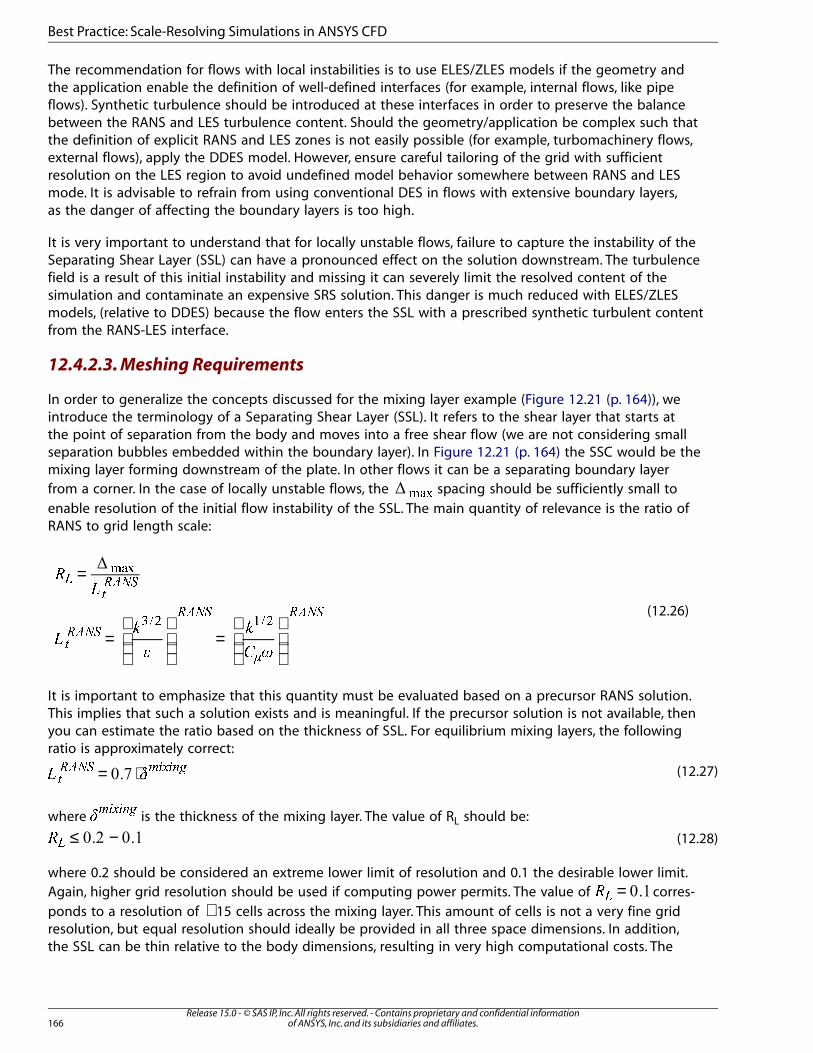
The recommendation for flows with local instabilities is to use ELES/ZLES models if the geometry andthe application enable the definition of well-defined interfaces (for example, internal flows, like pipeflows). Synthetic turbulence should be introduced at these interfaces in order to preserve the balancebetween the RANS and LES turbulence content. Should the geometry/application be complex such thatthe definition of explicit RANS and LES zones is not easily possible (for example, turbomachinery flows,external flows), apply the DDES model. However, ensure careful tailoring of the grid with sufficientresolution on the LES region to avoid undefined model behavior somewhere between RANS and LESmode. It is advisable to refrain from using conventional DES in flows with extensive boundary layers,as the danger of affecting the boundary layers is too high.
It is very important to understand that for locally unstable flows, failure to capture the instability of theSeparating Shear Layer (SSL) can have a pronounced effect on the solution downstream. The turbulencefield is a result of this initial instability and missing it can severely limit the resolved content of thesimulation and contaminate an expensive SRS solution. This danger is much reduced with ELES/ZLESmodels, (relative to DDES) because the flow enters the SSL with a prescribed synthetic turbulent contentfrom the RANS-LES interface.
12.4.2.3. Meshing Requirements
In order to generalize the concepts discussed for the mixing layer example (Figure 12.21 (p. 164)), weintroduce the terminology of a Separating Shear Layer (SSL). It refers to the shear layer that starts atthe point of separation from the body and moves into a free shear flow (we are not considering smallseparation bubbles embedded within the boundary layer). In Figure 12.21 (p. 164) the SSC would be themixing layer forming downstream of the plate. In other flows it can be a separating boundary layerfrom a corner. In the case of locally unstable flows, the ��� spacing should be sufficiently small toenable resolution of the initial flow instability of the SSL. The main quantity of relevance is the ratio ofRANS to grid length scale:
(12.26)
=
=
=
�
�
��
�
�
� �
�� �
�� �
�� �
�
�� �
���
��� ���
It is important to emphasize that this quantity must be evaluated based on a precursor RANS solution.This implies that such a solution exists and is meaningful. If the precursor solution is not available, thenyou can estimate the ratio based on the thickness of SSL. For equilibrium mixing layers, the followingratio is approximately correct:
(12.27)= ⋅� ������ �� �!"
where #$%&%'(
is the thickness of the mixing layer. The value of RL should be:
(12.28)≤ −)*
where 0.2 should be considered an extreme lower limit of resolution and 0.1 the desirable lower limit.Again, higher grid resolution should be used if computing power permits. The value of =+, corres-ponds to a resolution of ∼ 15 cells across the mixing layer. This amount of cells is not a very fine gridresolution, but equal resolution should ideally be provided in all three space dimensions. In addition,the SSL can be thin relative to the body dimensions, resulting in very high computational costs. The
Release 15.0 - © SAS IP, Inc. All rights reserved. - Contains proprietary and confidential informationof ANSYS, Inc. and its subsidiaries and affiliates.166
Best Practice: Scale-Resolving Simulations in ANSYS CFD
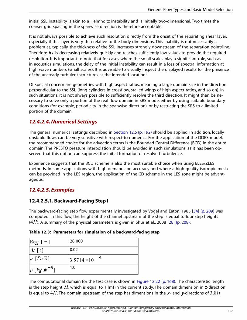
initial SSL instability is akin to a Helmholtz instability and is initially two-dimensional. Two times thecoarser grid spacing in the spanwise direction is therefore acceptable.
It is not always possible to achieve such resolution directly from the onset of the separating shear layer,especially if this layer is very thin relative to the body dimensions. This inability is not necessarily aproblem as, typically, the thickness of the SSL increases strongly downstream of the separation point/line.Therefore �� is decreasing relatively quickly and reaches sufficiently low values to provide the requiredresolution. It is important to note that for cases where the small scales play a significant role, such asin acoustics simulations, the delay of the initial instability can result in a loss of spectral information athigh wave numbers (small scales). It is advisable to visually inspect the displayed results for the presenceof the unsteady turbulent structures at the intended locations.
Of special concern are geometries with high aspect ratios, meaning a large domain size in the directionperpendicular to the SSL (long cylinders in crossflow, stalled wings of high aspect ratios, and so on). Insuch situations, it is not always possible to sufficiently resolve the third direction. It might then be ne-cessary to solve only a portion of the real flow domain in SRS mode, either by using suitable boundaryconditions (for example, periodicity in the spanwise direction), or by restricting the SRS to a limitedportion of the domain.
12.4.2.4. Numerical Settings
The general numerical settings described in Section 12.5 (p. 192) should be applied. In addition, locallyunstable flows can be very sensitive with respect to numerics. For the application of the DDES model,the recommended choice for the advection terms is the Bounded Central Difference (BCD) in the entiredomain. The PRESTO pressure interpolation should be avoided in such simulations, as it has been ob-served that this option can suppress the initial formation of resolved turbulence.
Experience suggests that the BCD scheme is also the most suitable choice when using ELES/ZLESmethods. In some applications with high demands on accuracy and where a high quality isotropic meshcan be provided in the LES region, the application of the CD scheme in the LES zone might be advant-ageous.
12.4.2.5. Examples
12.4.2.5.1. Backward-Facing Step I
The backward-facing step flow experimentally investigated by Vogel and Eaton, 1985 [34] (p. 209) wascomputed. In this flow, the height of the channel upstream of the step is equal to four step heights( �). A summary of the physical parameters is given in Shur et al., 2008 [26] (p. 208):
Table 12.3: Parameters for simulation of a backward-facing step
28 000−�
0.02�� �
× − �⋅� �
1.0⋅ −� � �
�
The computational domain for the test case is shown in Figure 12.22 (p. 168). The characteristic lengthis the step height, �, which is equal to 1 [m] in the current study. The domain dimension in �-directionis equal to �. The domain upstream of the step has dimensions in the �- and �-directions of �
167Release 15.0 - © SAS IP, Inc. All rights reserved. - Contains proprietary and confidential information
of ANSYS, Inc. and its subsidiaries and affiliates.
Generic Flow Types and Basic Model Selection

and � respectively. The downstream domain has dimensions in the �- and �-direction, of � and
� respectively.
Figure 12.22: The computational domain for the Backward-Facing Step test case
An example of the computational grid used for the test case is shown in Figure 12.23 (p. 169). The gridhas 2.25 million hexahedral cells (2.3 million nodes) providing a near-wall resolution in wall units to beless than one. A non-dimensional time step (based on step height and inlet velocity) of =� ensuresthat the CFL number is less than unity in the unsteady mixing zone downstream of the step. Thenumber of cells in the spanwise direction is 80. The solution was averaged over 5000 time steps.
In Figure 12.23 (b) (p. 169) all boundary conditions are shown. In the spanwise direction (cyan coloredboundary), a periodic boundary condition was applied; on the red-colored boundaries, no-slip wallconditions were applied; on the blue-colored boundary, an outlet condition was applied; and on thegreen-colored boundary, an inlet condition was applied. The latter was provided in the form of steady-state RANS profiles. Therefore, unsteadiness resulted solely from the local flow instability past the step.
Release 15.0 - © SAS IP, Inc. All rights reserved. - Contains proprietary and confidential informationof ANSYS, Inc. and its subsidiaries and affiliates.168
Best Practice: Scale-Resolving Simulations in ANSYS CFD
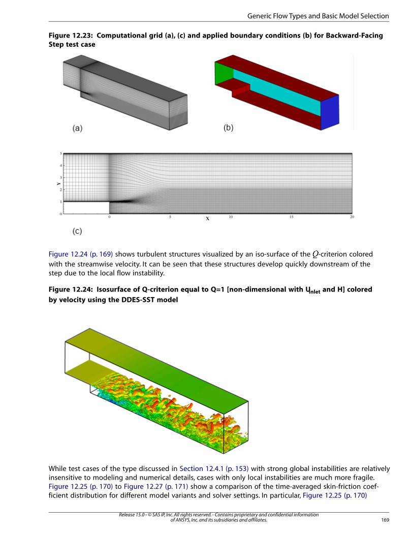
Figure 12.23: Computational grid (a), (c) and applied boundary conditions (b) for Backward-Facing
Step test case
Figure 12.24 (p. 169) shows turbulent structures visualized by an iso-surface of the �-criterion coloredwith the streamwise velocity. It can be seen that these structures develop quickly downstream of thestep due to the local flow instability.
Figure 12.24: Isosurface of Q-criterion equal to Q=1 [non-dimensional with Uinlet and H] colored
by velocity using the DDES-SST model
While test cases of the type discussed in Section 12.4.1 (p. 153) with strong global instabilities are relativelyinsensitive to modeling and numerical details, cases with only local instabilities are much more fragile.Figure 12.25 (p. 170) to Figure 12.27 (p. 171) show a comparison of the time-averaged skin-friction coef-ficient distribution for different model variants and solver settings. In particular, Figure 12.25 (p. 170)
169Release 15.0 - © SAS IP, Inc. All rights reserved. - Contains proprietary and confidential information
of ANSYS, Inc. and its subsidiaries and affiliates.
Generic Flow Types and Basic Model Selection
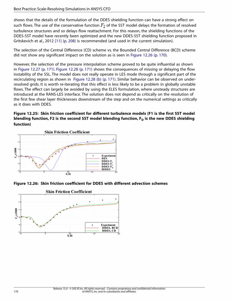
shows that the details of the formulation of the DDES shielding function can have a strong effect onsuch flows. The use of the conservative function �� of the SST model delays the formation of resolvedturbulence structures and so delays flow reattachment. For this reason, the shielding functions of theDDES-SST model have recently been optimized and the new DDES-SST shielding function proposed inGritskevich et al., 2012 [11] (p. 208) is recommended (and used in the current simulation).
The selection of the Central Difference (CD) scheme vs. the Bounded Central Difference (BCD) schemedid not show any significant impact on the solution as is seen in Figure 12.26 (p. 170).
However, the selection of the pressure interpolation scheme proved to be quite influential as shownin Figure 12.27 (p. 171). Figure 12.28 (p. 171) shows the consequences of missing or delaying the flowinstability of the SSL. The model does not really operate in LES mode through a significant part of therecirculating region as shown in Figure 12.28 (b) (p. 171). Similar behavior can be observed on under-resolved grids. It is worth re-iterating that this effect is less likely to be a problem in globally unstableflows. The effect can largely be avoided by using the ELES formulation, where unsteady structures areintroduced at the RANS-LES interface. The solution does not depend as critically on the resolution ofthe first few shear layer thicknesses downstream of the step and on the numerical settings as criticallyas it does with DDES.
Figure 12.25: Skin friction coefficient for different turbulence models (F1 is the first SST model
blending function, F2 is the second SST model blending function, FD is the new DDES shielding
function)
Figure 12.26: Skin friction coefficient for DDES with different advection schemes
Release 15.0 - © SAS IP, Inc. All rights reserved. - Contains proprietary and confidential informationof ANSYS, Inc. and its subsidiaries and affiliates.170
Best Practice: Scale-Resolving Simulations in ANSYS CFD
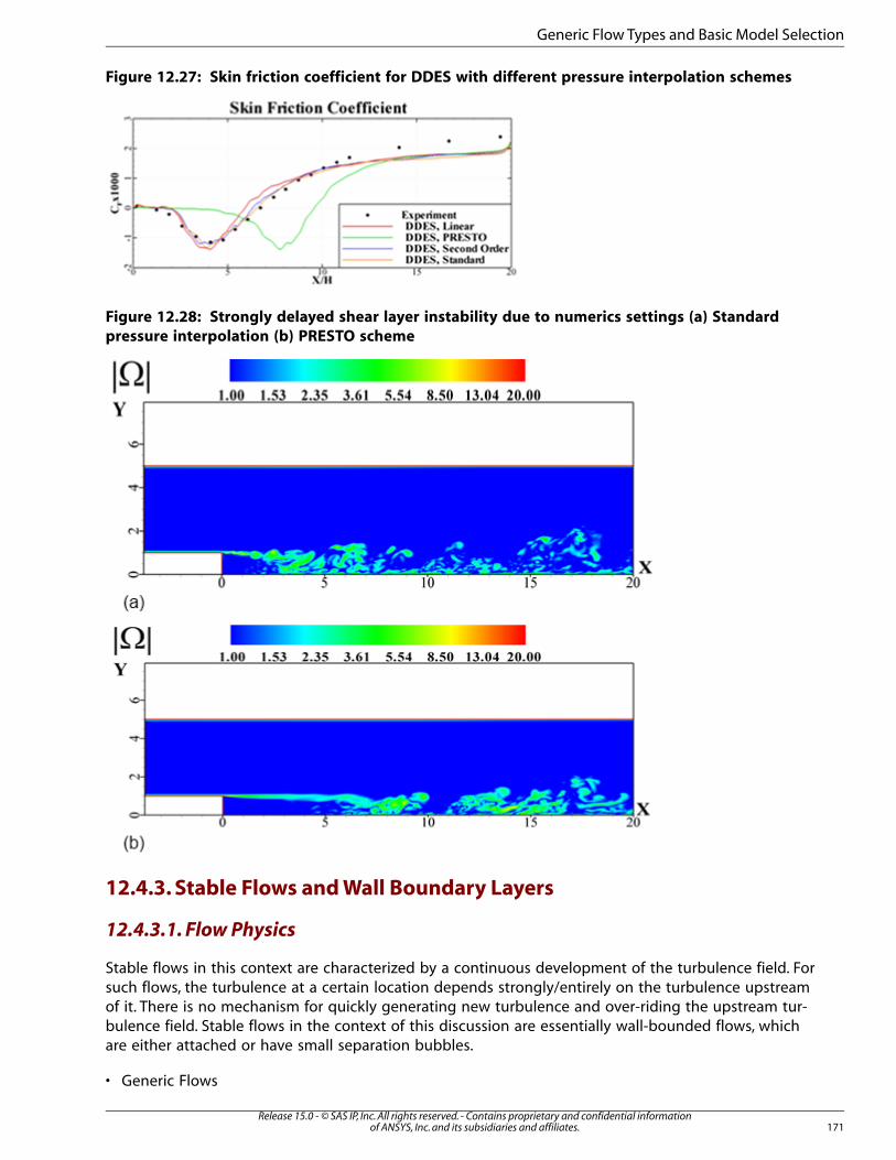
Figure 12.27: Skin friction coefficient for DDES with different pressure interpolation schemes
Figure 12.28: Strongly delayed shear layer instability due to numerics settings (a) Standard
pressure interpolation (b) PRESTO scheme
12.4.3. Stable Flows and Wall Boundary Layers
12.4.3.1. Flow Physics
Stable flows in this context are characterized by a continuous development of the turbulence field. Forsuch flows, the turbulence at a certain location depends strongly/entirely on the turbulence upstreamof it. There is no mechanism for quickly generating new turbulence and over-riding the upstream tur-bulence field. Stable flows in the context of this discussion are essentially wall-bounded flows, whichare either attached or have small separation bubbles.
• Generic Flows
171Release 15.0 - © SAS IP, Inc. All rights reserved. - Contains proprietary and confidential information
of ANSYS, Inc. and its subsidiaries and affiliates.
Generic Flow Types and Basic Model Selection
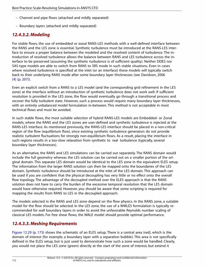
– Channel and pipe flows (attached and mildly separated)
– Boundary layers (attached and mildly separated)
12.4.3.2. Modeling
For stable flows, the use of embedded or zonal RANS-LES methods with a well-defined interface betweenthe RANS and the LES zone is essential. Synthetic turbulence must be introduced at the RANS-LES inter-face to ensure a proper balance between the modeled and the resolved content of turbulence. The in-troduction of resolved turbulence allows the balance between RANS and LES turbulence across the in-terface to be preserved (assuming the synthetic turbulence is of sufficient quality). Neither DDES norSAS-type models are able to switch from RANS to SRS mode in such stable situations. Even in caseswhere resolved turbulence is specified at the inlet (or an interface) these models will typically switchback to their underlying RANS mode after some boundary layer thicknesses (see Davidson, 2006[4] (p. 207)).
Even an explicit switch from a RANS to a LES model (and the corresponding grid refinement in the LESzone) at the interface without an introduction of synthetic turbulence does not work well. If sufficientresolution is provided in the LES zone, the flow would eventually go through a transitional process andrecover the fully turbulent state. However, such a process would require many boundary layer thicknesses,with an entirely unbalanced model formulation in-between. This method is not acceptable in mosttechnical flows and must be avoided.
In such stable flows, the most suitable selection of hybrid RANS-LES models are Embedded- or Zonalmodels, where the RANS and the LES zones are user-defined and synthetic turbulence is injected at theRANS-LES interface. As mentioned previously, the RANS-LES interface should be placed in a non-criticalregion of the flow (equilibrium flow), since existing synthetic turbulence generators do not providerealistic turbulent fluctuations for strongly non-equilibrium flows. As a result, placing the interface insuch regions results in a too-slow relaxation from synthetic to real turbulence (typically, severalboundary layer thicknesses).
As an alternative, the RANS and LES simulations can be carried out separately. The RANS domain wouldinclude the full geometry whereas the LES solution can be carried out on a smaller portion of the ori-ginal domain. This separate LES domain would be identical to the LES zone in the equivalent ELES setup.The information from the larger RANS solution can then be mapped onto the boundaries of the LESdomain. Synthetic turbulence should be introduced at the inlet of the LES domain. This approach canbe used if you are confident that the physical decoupling has very little or no effect onto the overallflow topology. The advantage of the decoupled method over the ELES approach is that the RANSsolution does not have to carry the burden of the excessive temporal resolution that the LES domainwould have otherwise required. However, you should be aware that some scripting is required formapping the results from RANS to LES in the decoupled approach.
The models selected in the RANS and LES zone depend on the flow physics. In the RANS zone, a suitablemodel for the flow should be selected. In the LES zone, the use of a WMLES formulation is typically re-commended for wall boundary layers in order to avoid the unfavorable Reynolds number scaling ofclassical LES models. For free shear flows, the WALE model should provide optimal performance.
12.4.3.3. Meshing Requirements
Figure 12.29 (p. 173) shows the schematic of an ELES setup. There is a central area (red), which is thedomain of interest (for example, a boundary layer with a separation bubble). This area is not specificallydefined in the ELES setup, but is just used to demonstrate how such a zone would be handled. Clearly,you would not place the LES zone (green) directly at the start of the zone of interest, but extend it
Release 15.0 - © SAS IP, Inc. All rights reserved. - Contains proprietary and confidential informationof ANSYS, Inc. and its subsidiaries and affiliates.172
Best Practice: Scale-Resolving Simulations in ANSYS CFD
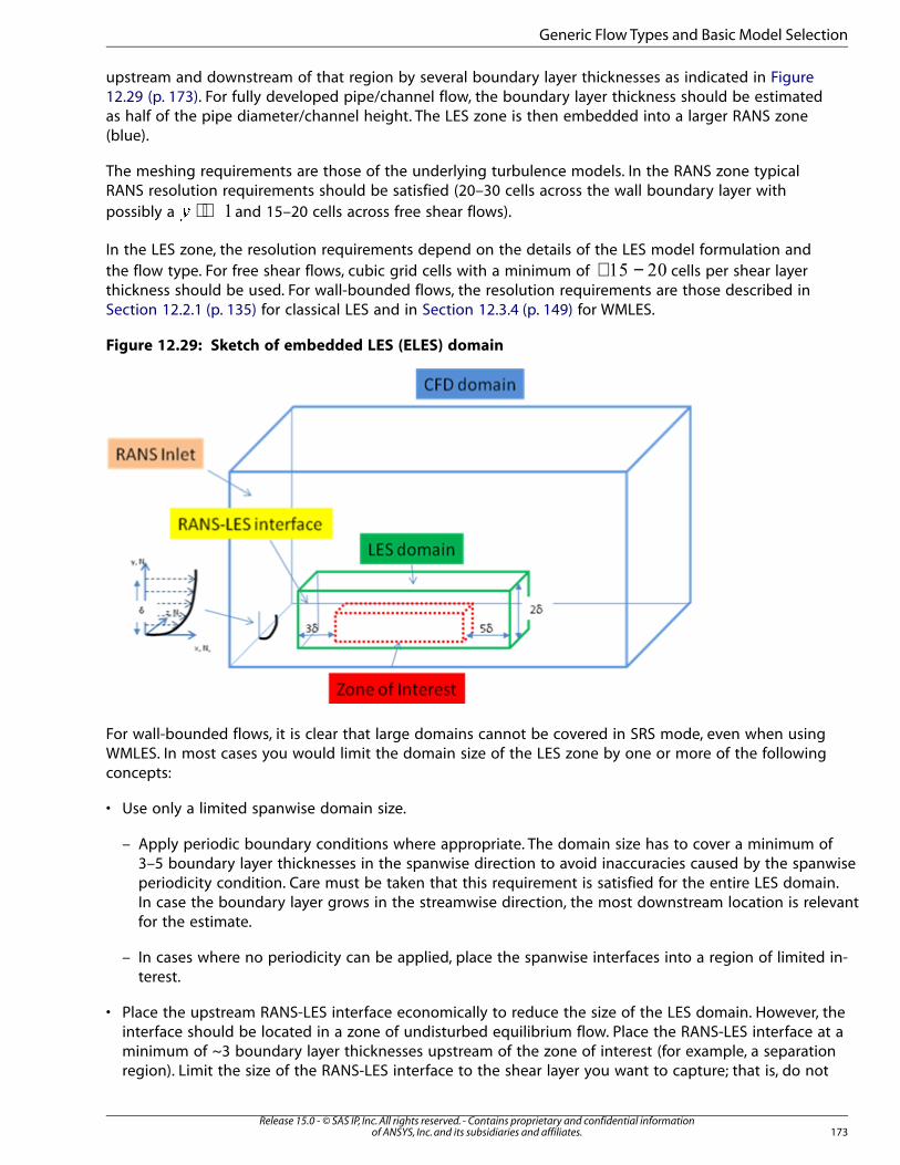
upstream and downstream of that region by several boundary layer thicknesses as indicated in Figure12.29 (p. 173). For fully developed pipe/channel flow, the boundary layer thickness should be estimatedas half of the pipe diameter/channel height. The LES zone is then embedded into a larger RANS zone(blue).
The meshing requirements are those of the underlying turbulence models. In the RANS zone typicalRANS resolution requirements should be satisfied (20–30 cells across the wall boundary layer withpossibly a + ∼� and 15–20 cells across free shear flows).
In the LES zone, the resolution requirements depend on the details of the LES model formulation andthe flow type. For free shear flows, cubic grid cells with a minimum of ∼ − cells per shear layerthickness should be used. For wall-bounded flows, the resolution requirements are those described inSection 12.2.1 (p. 135) for classical LES and in Section 12.3.4 (p. 149) for WMLES.
Figure 12.29: Sketch of embedded LES (ELES) domain
For wall-bounded flows, it is clear that large domains cannot be covered in SRS mode, even when usingWMLES. In most cases you would limit the domain size of the LES zone by one or more of the followingconcepts:
• Use only a limited spanwise domain size.
– Apply periodic boundary conditions where appropriate. The domain size has to cover a minimum of3–5 boundary layer thicknesses in the spanwise direction to avoid inaccuracies caused by the spanwiseperiodicity condition. Care must be taken that this requirement is satisfied for the entire LES domain.In case the boundary layer grows in the streamwise direction, the most downstream location is relevantfor the estimate.
– In cases where no periodicity can be applied, place the spanwise interfaces into a region of limited in-terest.
• Place the upstream RANS-LES interface economically to reduce the size of the LES domain. However, theinterface should be located in a zone of undisturbed equilibrium flow. Place the RANS-LES interface at aminimum of ~3 boundary layer thicknesses upstream of the zone of interest (for example, a separationregion). Limit the size of the RANS-LES interface to the shear layer you want to capture; that is, do not
173Release 15.0 - © SAS IP, Inc. All rights reserved. - Contains proprietary and confidential information
of ANSYS, Inc. and its subsidiaries and affiliates.
Generic Flow Types and Basic Model Selection
extend the interface far into the freestream, as the code will then generate resolved turbulence in freestreamregions where no LES is required. The Vortex Method (VM) would also generate a large number of vorticesif the RANS-LES interface were too large.
• Place the downstream LES-RANS interface economically to reduce the size of LES domain. However, donot place the interface immediately downstream of the zone of interest, but place it several boundarylayer thicknesses farther downstream to avoid any negative influence of the downstream RANS model(this approach enables the boundary layer to recover several boundary layer thicknesses downstream ofa separation before switching back to RANS)
• Limit the height of the LES zone, but allow for some space above the boundary layer. Typically the LESzone should be about twice as thick as the boundary layer.
In order to check the quality of the simulation, sensitive quantities like time-averaged wall shear stressshould be plotted across the RANS-LES zones. There should be no large jump in those quantities andthe unavoidable disturbance caused by the interface should be recovered before entering the zone ofinterest.
12.4.3.4. Numerical Settings
Zonal methods typically enable a separate selection of numerical settings in the RANS and LES zones.For very sensitive simulations, you can therefore select a pure Central Difference (CD) in the LES domain,while using an appropriate numerical scheme in the RANS parts. However, you can also select a globalscheme, in which case the Bounded Central Difference (BCD) scheme is recommended.
12.4.3.5. Examples
12.4.3.5.1. Periodic Channel
The periodic channel flow is not an ELES, but a WMLES application. This section of the report showsthat as WMLES is typically used in the LES portion of ELES/ZLES applications. The entire domain isWMLES and there are no RANS-LES interfaces. Simulations of this flow have been carried out assumingincompressible fluid at several Reynolds numbers based on friction velocity �
� and channel height
=� � , Re = 395, 760, 1100, 2400, and 18000. The flow is driven by a constant pressure gradient
= − ⋅ ⋅�� �� � � �
, where � is the pressure and � is the density. This pressure gradient is taken
into account in the governing equations via a source term in the momentum equations, which allowsimposing periodic boundary conditions not only in the spanwise direction , but also in the streamwisedirection �. Note that within such an approach, the bulk velocity of the flow is not specified and shouldbe obtained as a part of the solution, which means that it could be different with different turbulencemodels. Alternatively, you can specify the mass flow and the solver will adjust the imposed pressuregradient accordingly.
The size of the computational domain shown in Figure 12.30 (p. 175) is equal to � in the streamwisedirection and � in the spanwise direction. For all considered Reynolds numbers, the computationalgrid is unchanged in the streamwise and spanwise directions with a uniform grid-spacing of �
and � respectively. This gives 10 cells per channel half width, =� � , (� being the relevant
boundary layer thickness) in the streamwise and 20 cells per � in the spanwise direction. Different grids
have been used in the wall-normal direction. This arrangement provides a sufficient resolution ( <+��
near the wall) at different Reynolds numbers. Note, however, that all simulations could have been per-
formed on the finest grid. The non-dimensional time step is =� � � , which ensures that theCFL number is <��� in the entire domain. The solution was averaged in time over 5000 time steps.
Release 15.0 - © SAS IP, Inc. All rights reserved. - Contains proprietary and confidential informationof ANSYS, Inc. and its subsidiaries and affiliates.174
Best Practice: Scale-Resolving Simulations in ANSYS CFD
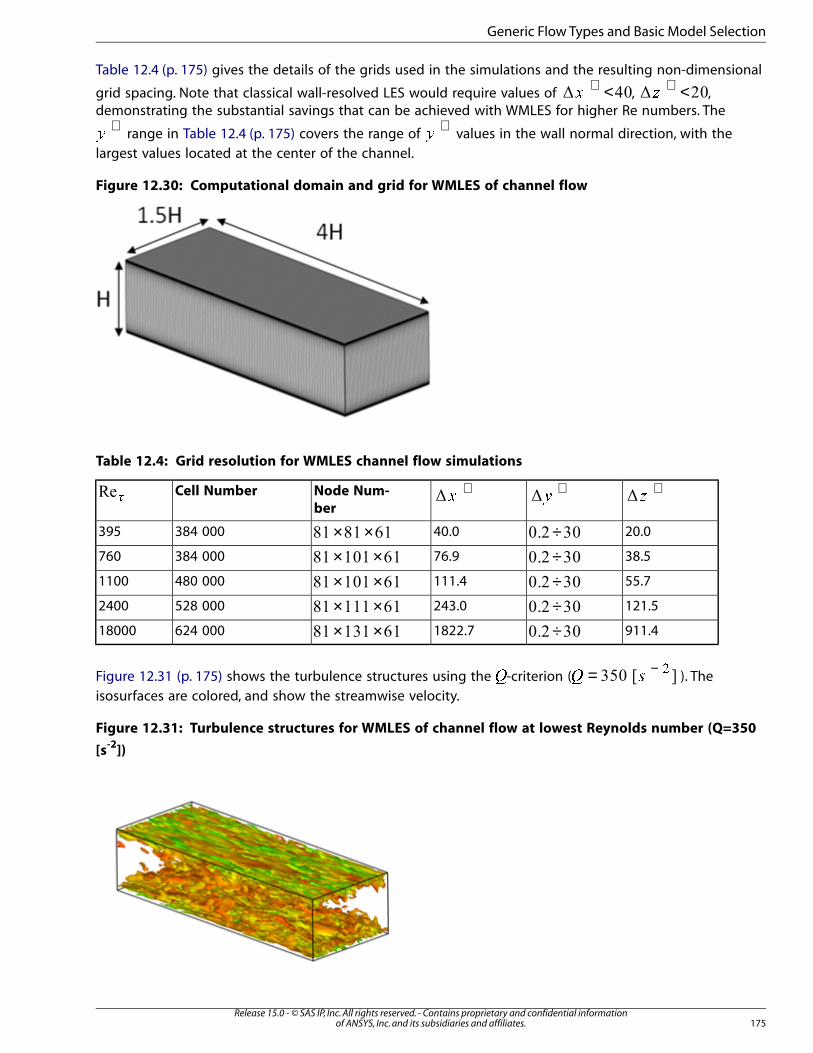
Table 12.4 (p. 175) gives the details of the grids used in the simulations and the resulting non-dimensional
grid spacing. Note that classical wall-resolved LES would require values of <+� , <+
� ,demonstrating the substantial savings that can be achieved with WMLES for higher Re numbers. The
+� range in Table 12.4 (p. 175) covers the range of
+� values in the wall normal direction, with the
largest values located at the center of the channel.
Figure 12.30: Computational domain and grid for WMLES of channel flow
Table 12.4: Grid resolution for WMLES channel flow simulations
+�
+�
+�Node Num-
ber
Cell Number�
20.0÷40.0× ×384 000395
38.5÷76.9× ×384 000760
55.7÷111.4× ×480 0001100
121.5÷243.0× ×528 0002400
911.4÷1822.7× ×624 00018000
Figure 12.31 (p. 175) shows the turbulence structures using the �-criterion ( = −
�). The
isosurfaces are colored, and show the streamwise velocity.
Figure 12.31: Turbulence structures for WMLES of channel flow at lowest Reynolds number (Q=350
[s-2
])
175Release 15.0 - © SAS IP, Inc. All rights reserved. - Contains proprietary and confidential information
of ANSYS, Inc. and its subsidiaries and affiliates.
Generic Flow Types and Basic Model Selection
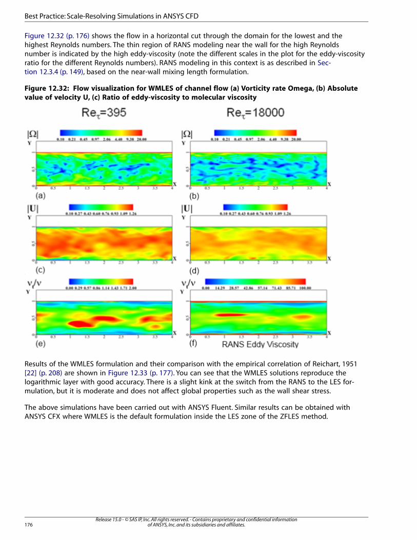
Figure 12.32 (p. 176) shows the flow in a horizontal cut through the domain for the lowest and thehighest Reynolds numbers. The thin region of RANS modeling near the wall for the high Reynoldsnumber is indicated by the high eddy-viscosity (note the different scales in the plot for the eddy-viscosityratio for the different Reynolds numbers). RANS modeling in this context is as described in Sec-tion 12.3.4 (p. 149), based on the near-wall mixing length formulation.
Figure 12.32: Flow visualization for WMLES of channel flow (a) Vorticity rate Omega, (b) Absolute
value of velocity U, (c) Ratio of eddy-viscosity to molecular viscosity
Results of the WMLES formulation and their comparison with the empirical correlation of Reichart, 1951[22] (p. 208) are shown in Figure 12.33 (p. 177). You can see that the WMLES solutions reproduce thelogarithmic layer with good accuracy. There is a slight kink at the switch from the RANS to the LES for-mulation, but it is moderate and does not affect global properties such as the wall shear stress.
The above simulations have been carried out with ANSYS Fluent. Similar results can be obtained withANSYS CFX where WMLES is the default formulation inside the LES zone of the ZFLES method.
Release 15.0 - © SAS IP, Inc. All rights reserved. - Contains proprietary and confidential informationof ANSYS, Inc. and its subsidiaries and affiliates.176
Best Practice: Scale-Resolving Simulations in ANSYS CFD
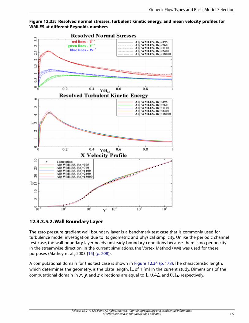
Figure 12.33: Resolved normal stresses, turbulent kinetic energy, and mean velocity profiles for
WMLES at different Reynolds numbers
12.4.3.5.2. Wall Boundary Layer
The zero pressure gradient wall boundary layer is a benchmark test case that is commonly used forturbulence model investigation due to its geometric and physical simplicity. Unlike the periodic channeltest case, the wall boundary layer needs unsteady boundary conditions because there is no periodicityin the streamwise direction. In the current simulations, the Vortex Method (VM) was used for thesepurposes (Mathey et al., 2003 [15] (p. 208)).
A computational domain for this test case is shown in Figure 12.34 (p. 178). The characteristic length,which determines the geometry, is the plate length, , of 1 [m] in the current study. Dimensions of thecomputational domain in �, �, and � directions are equal to , �, and � respectively.
177Release 15.0 - © SAS IP, Inc. All rights reserved. - Contains proprietary and confidential information
of ANSYS, Inc. and its subsidiaries and affiliates.
Generic Flow Types and Basic Model Selection
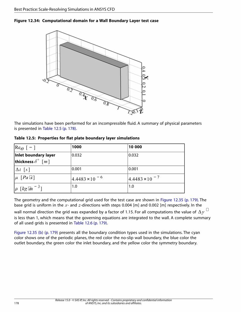
Figure 12.34: Computational domain for a Wall Boundary Layer test case
The simulations have been performed for an incompressible fluid. A summary of physical parametersis presented in Table 12.5 (p. 178).
Table 12.5: Properties for flat plate boundary layer simulations
10 0001000−�
0.0320.032Inlet boundary layer
thickness o
� �
0.0010.001� �
× − �× − �⋅� �
1.01.0⋅ −� � �
�
The geometry and the computational grid used for the test case are shown in Figure 12.35 (p. 179). Thebase grid is uniform in the �- and �-directions with steps 0.004 [m] and 0.002 [m] respectively. In the
wall normal direction the grid was expanded by a factor of 1.15. For all computations the value of +
�
is less than 1, which means that the governing equations are integrated to the wall. A complete summaryof all used grids is presented in Table 12.6 (p. 179).
Figure 12.35 (b) (p. 179) presents all the boundary condition types used in the simulations. The cyancolor shows one of the periodic planes, the red color the no-slip wall boundary, the blue color theoutlet boundary, the green color the inlet boundary, and the yellow color the symmetry boundary.
Release 15.0 - © SAS IP, Inc. All rights reserved. - Contains proprietary and confidential informationof ANSYS, Inc. and its subsidiaries and affiliates.178
Best Practice: Scale-Resolving Simulations in ANSYS CFD
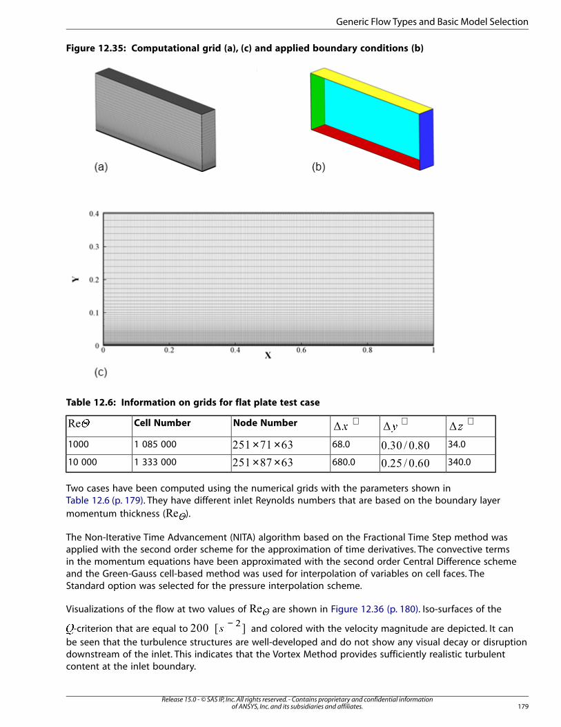
Figure 12.35: Computational grid (a), (c) and applied boundary conditions (b)
Table 12.6: Information on grids for flat plate test case
+�
+�
+�Node NumberCell Number�
34.068.0× ×1 085 0001000
340.0680.0× ×1 333 00010 000
Two cases have been computed using the numerical grids with the parameters shown inTable 12.6 (p. 179). They have different inlet Reynolds numbers that are based on the boundary layermomentum thickness ( �).
The Non-Iterative Time Advancement (NITA) algorithm based on the Fractional Time Step method wasapplied with the second order scheme for the approximation of time derivatives. The convective termsin the momentum equations have been approximated with the second order Central Difference schemeand the Green-Gauss cell-based method was used for interpolation of variables on cell faces. TheStandard option was selected for the pressure interpolation scheme.
Visualizations of the flow at two values of � are shown in Figure 12.36 (p. 180). Iso-surfaces of the
�-criterion that are equal to −
��
and colored with the velocity magnitude are depicted. It canbe seen that the turbulence structures are well-developed and do not show any visual decay or disruptiondownstream of the inlet. This indicates that the Vortex Method provides sufficiently realistic turbulentcontent at the inlet boundary.
179Release 15.0 - © SAS IP, Inc. All rights reserved. - Contains proprietary and confidential information
of ANSYS, Inc. and its subsidiaries and affiliates.
Generic Flow Types and Basic Model Selection
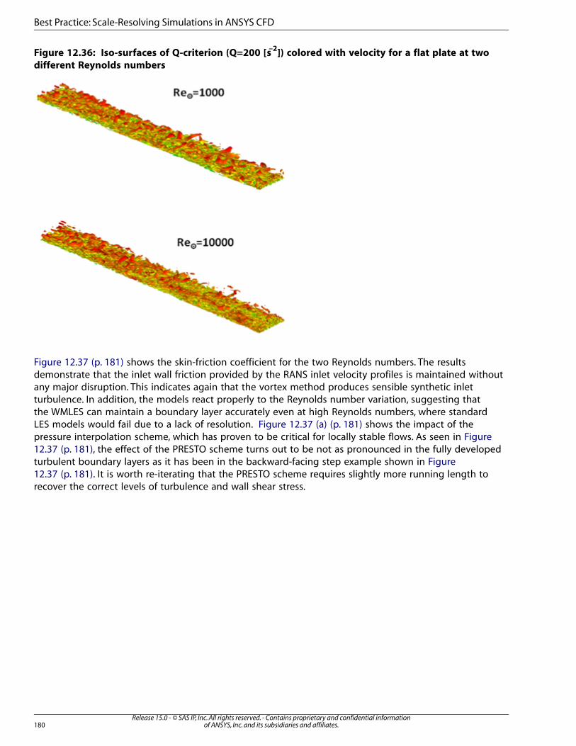
Figure 12.36: Iso-surfaces of Q-criterion (Q=200 [s–2
]) colored with velocity for a flat plate at two
different Reynolds numbers
Figure 12.37 (p. 181) shows the skin-friction coefficient for the two Reynolds numbers. The resultsdemonstrate that the inlet wall friction provided by the RANS inlet velocity profiles is maintained withoutany major disruption. This indicates again that the vortex method produces sensible synthetic inletturbulence. In addition, the models react properly to the Reynolds number variation, suggesting thatthe WMLES can maintain a boundary layer accurately even at high Reynolds numbers, where standardLES models would fail due to a lack of resolution. Figure 12.37 (a) (p. 181) shows the impact of thepressure interpolation scheme, which has proven to be critical for locally stable flows. As seen in Figure12.37 (p. 181), the effect of the PRESTO scheme turns out to be not as pronounced in the fully developedturbulent boundary layers as it has been in the backward-facing step example shown in Figure12.37 (p. 181). It is worth re-iterating that the PRESTO scheme requires slightly more running length torecover the correct levels of turbulence and wall shear stress.
Release 15.0 - © SAS IP, Inc. All rights reserved. - Contains proprietary and confidential informationof ANSYS, Inc. and its subsidiaries and affiliates.180
Best Practice: Scale-Resolving Simulations in ANSYS CFD
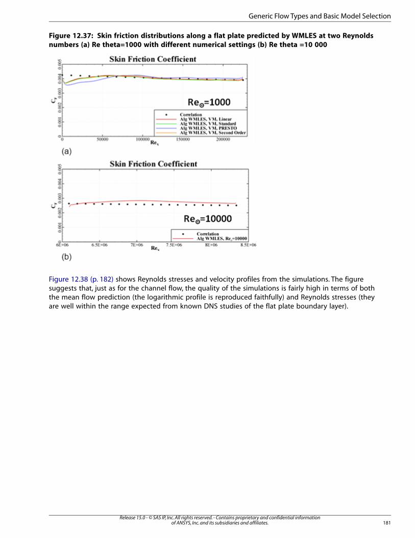
Figure 12.37: Skin friction distributions along a flat plate predicted by WMLES at two Reynolds
numbers (a) Re theta=1000 with different numerical settings (b) Re theta =10 000
Figure 12.38 (p. 182) shows Reynolds stresses and velocity profiles from the simulations. The figuresuggests that, just as for the channel flow, the quality of the simulations is fairly high in terms of boththe mean flow prediction (the logarithmic profile is reproduced faithfully) and Reynolds stresses (theyare well within the range expected from known DNS studies of the flat plate boundary layer).
181Release 15.0 - © SAS IP, Inc. All rights reserved. - Contains proprietary and confidential information
of ANSYS, Inc. and its subsidiaries and affiliates.
Generic Flow Types and Basic Model Selection

Figure 12.38: Profiles of resolved normal and shear Reynolds stresses and mean velocity in the
flat plate boundary layer predicted by WMLES at two Reynolds numbers (a) Re theta=1000 with
different numerical settings (b) Re theta=10 000 with the second order pressure interpolation
The above simulations have been carried out with ANSYS Fluent. Similar results can be obtained withANSYS CFX where WMLES is the default formulation inside the LES zone of the ZFLES method.
12.4.3.5.3. NASA Hump Flow
A challenging test case for ELES in combination with WMLES was computed within the EU projectATAAC. The case models the flow over a hump with a relatively large separation zone on the leewardside. Figure 12.39 (p. 182) shows the experimental setup (Greenblatt et al., 2005). Due to the limitedseparation zone, this flow would be categorized as a stable flow in the present context.
Figure 12.39: Experimental setup for NASA hump flow experiment
Release 15.0 - © SAS IP, Inc. All rights reserved. - Contains proprietary and confidential informationof ANSYS, Inc. and its subsidiaries and affiliates.182
Best Practice: Scale-Resolving Simulations in ANSYS CFD
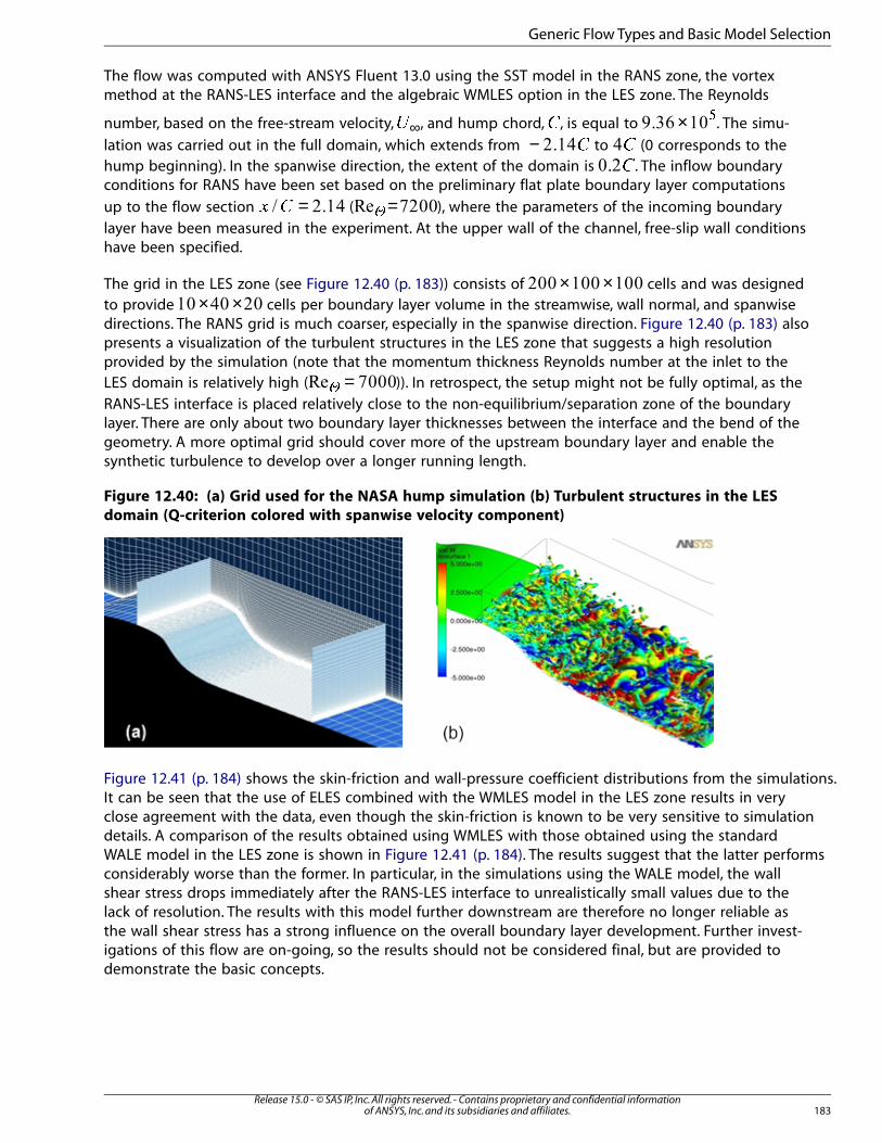
The flow was computed with ANSYS Fluent 13.0 using the SST model in the RANS zone, the vortexmethod at the RANS-LES interface and the algebraic WMLES option in the LES zone. The Reynolds
number, based on the free-stream velocity, ∞� , and hump chord,�, is equal to × �. The simu-
lation was carried out in the full domain, which extends from − � to � (0 corresponds to thehump beginning). In the spanwise direction, the extent of the domain is �. The inflow boundaryconditions for RANS have been set based on the preliminary flat plate boundary layer computations
up to the flow section =� � ( =� ), where the parameters of the incoming boundarylayer have been measured in the experiment. At the upper wall of the channel, free-slip wall conditionshave been specified.
The grid in the LES zone (see Figure 12.40 (p. 183)) consists of × × cells and was designedto provide × × cells per boundary layer volume in the streamwise, wall normal, and spanwisedirections. The RANS grid is much coarser, especially in the spanwise direction. Figure 12.40 (p. 183) alsopresents a visualization of the turbulent structures in the LES zone that suggests a high resolutionprovided by the simulation (note that the momentum thickness Reynolds number at the inlet to theLES domain is relatively high ( = )). In retrospect, the setup might not be fully optimal, as theRANS-LES interface is placed relatively close to the non-equilibrium/separation zone of the boundarylayer. There are only about two boundary layer thicknesses between the interface and the bend of thegeometry. A more optimal grid should cover more of the upstream boundary layer and enable thesynthetic turbulence to develop over a longer running length.
Figure 12.40: (a) Grid used for the NASA hump simulation (b) Turbulent structures in the LES
domain (Q-criterion colored with spanwise velocity component)
Figure 12.41 (p. 184) shows the skin-friction and wall-pressure coefficient distributions from the simulations.It can be seen that the use of ELES combined with the WMLES model in the LES zone results in veryclose agreement with the data, even though the skin-friction is known to be very sensitive to simulationdetails. A comparison of the results obtained using WMLES with those obtained using the standardWALE model in the LES zone is shown in Figure 12.41 (p. 184). The results suggest that the latter performsconsiderably worse than the former. In particular, in the simulations using the WALE model, the wallshear stress drops immediately after the RANS-LES interface to unrealistically small values due to thelack of resolution. The results with this model further downstream are therefore no longer reliable asthe wall shear stress has a strong influence on the overall boundary layer development. Further invest-igations of this flow are on-going, so the results should not be considered final, but are provided todemonstrate the basic concepts.
183Release 15.0 - © SAS IP, Inc. All rights reserved. - Contains proprietary and confidential information
of ANSYS, Inc. and its subsidiaries and affiliates.
Generic Flow Types and Basic Model Selection
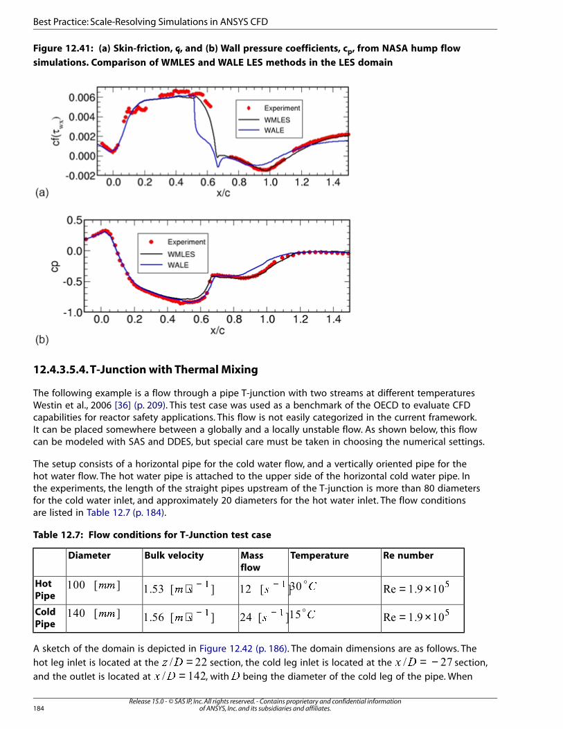
Figure 12.41: (a) Skin-friction, cf, and (b) Wall pressure coefficients, cp, from NASA hump flow
simulations. Comparison of WMLES and WALE LES methods in the LES domain
12.4.3.5.4. T-Junction with Thermal Mixing
The following example is a flow through a pipe T-junction with two streams at different temperaturesWestin et al., 2006 [36] (p. 209). This test case was used as a benchmark of the OECD to evaluate CFDcapabilities for reactor safety applications. This flow is not easily categorized in the current framework.It can be placed somewhere between a globally and a locally unstable flow. As shown below, this flowcan be modeled with SAS and DDES, but special care must be taken in choosing the numerical settings.
The setup consists of a horizontal pipe for the cold water flow, and a vertically oriented pipe for thehot water flow. The hot water pipe is attached to the upper side of the horizontal cold water pipe. Inthe experiments, the length of the straight pipes upstream of the T-junction is more than 80 diametersfor the cold water inlet, and approximately 20 diameters for the hot water inlet. The flow conditionsare listed in Table 12.7 (p. 184).
Table 12.7: Flow conditions for T-Junction test case
Re numberTemperatureMass
flow
Bulk velocityDiameter
= × �o�−
��⋅ −
� ����Hot
Pipe
= × �o−
�⋅ −
� ���Cold
Pipe
A sketch of the domain is depicted in Figure 12.42 (p. 186). The domain dimensions are as follows. The
hot leg inlet is located at the =� � section, the cold leg inlet is located at the = −� � section,
and the outlet is located at =� � , with � being the diameter of the cold leg of the pipe. When
Release 15.0 - © SAS IP, Inc. All rights reserved. - Contains proprietary and confidential informationof ANSYS, Inc. and its subsidiaries and affiliates.184
Best Practice: Scale-Resolving Simulations in ANSYS CFD
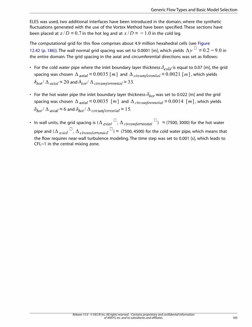
ELES was used, two additional interfaces have been introduced in the domain, where the syntheticfluctuations generated with the use of the Vortex Method have been specified. These sections have
been placed at =� � in the hot leg and at = −� � in the cold leg.
The computational grid for this flow comprises about 4.9 million hexahedral cells (see Figure
12.42 (p. 186)). The wall normal grid spacing was set to 0.0001 [m], which yields = −+� in
the entire domain. The grid spacing in the axial and circumferential directions was set as follows:
• For the cold water pipe where the inlet boundary layer thickness ���� is equal to 0.07 [m], the grid
spacing was chosen = �� �� and = ���������������� , which yields
≈���� � !�" and ≈#$%& '()'*+,-))-.&(/0 .
• For the hot water pipe the inlet boundary layer thickness 1234 was set to 0.022 [m] and the grid
spacing was chosen = 567869 and = :;<=;>?@A==ABC<DE , which yields
≈FGHI JKLJM and ≈NOPQ RSTRUVWXTTXYQSZ[ .
• In wall units, the grid spacing is (+
\]^\_ ,+
`ab`cdefbbfghaij ) ≈ (7500, 3000) for the hot water
pipe and (+
klmkn ,+
opqorstuqquvwpxy ) ≈ (7500, 4500) for the cold water pipe, which means that
the flow requires near-wall turbulence modeling. The time step was set to 0.001 [s], which leads toCFL~1 in the central mixing zone.
185Release 15.0 - © SAS IP, Inc. All rights reserved. - Contains proprietary and confidential information
of ANSYS, Inc. and its subsidiaries and affiliates.
Generic Flow Types and Basic Model Selection
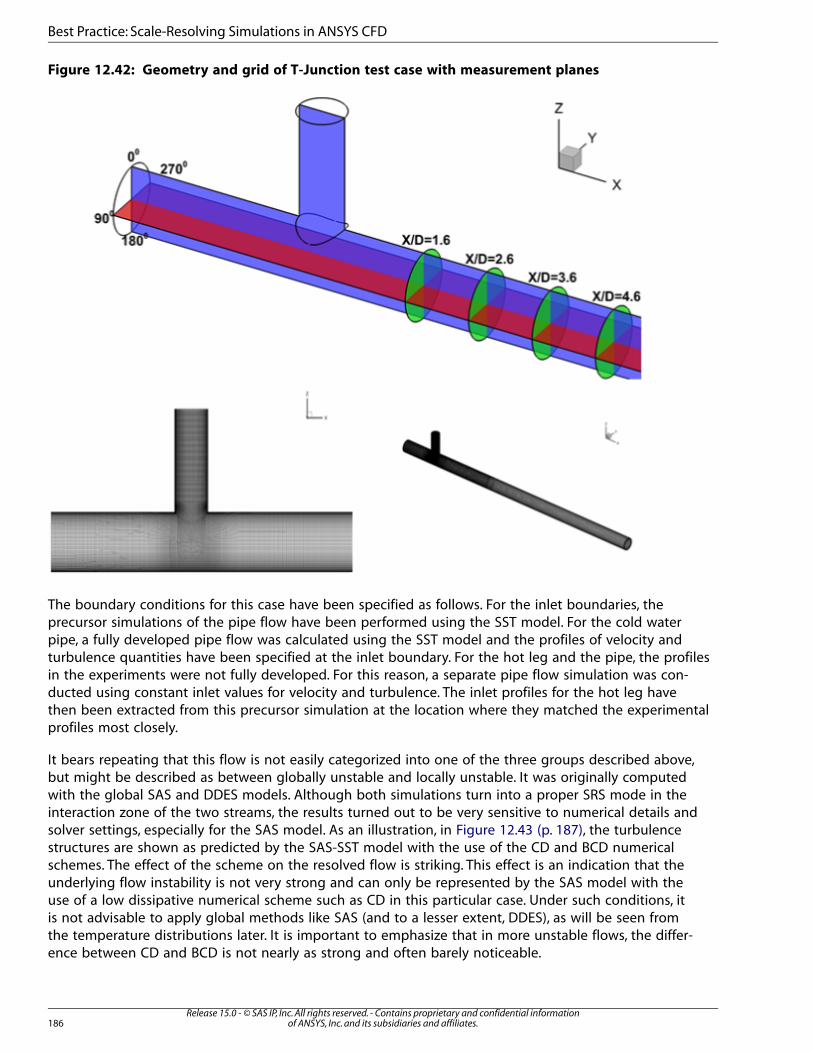
Figure 12.42: Geometry and grid of T-Junction test case with measurement planes
The boundary conditions for this case have been specified as follows. For the inlet boundaries, theprecursor simulations of the pipe flow have been performed using the SST model. For the cold waterpipe, a fully developed pipe flow was calculated using the SST model and the profiles of velocity andturbulence quantities have been specified at the inlet boundary. For the hot leg and the pipe, the profilesin the experiments were not fully developed. For this reason, a separate pipe flow simulation was con-ducted using constant inlet values for velocity and turbulence. The inlet profiles for the hot leg havethen been extracted from this precursor simulation at the location where they matched the experimentalprofiles most closely.
It bears repeating that this flow is not easily categorized into one of the three groups described above,but might be described as between globally unstable and locally unstable. It was originally computedwith the global SAS and DDES models. Although both simulations turn into a proper SRS mode in theinteraction zone of the two streams, the results turned out to be very sensitive to numerical details andsolver settings, especially for the SAS model. As an illustration, in Figure 12.43 (p. 187), the turbulencestructures are shown as predicted by the SAS-SST model with the use of the CD and BCD numericalschemes. The effect of the scheme on the resolved flow is striking. This effect is an indication that theunderlying flow instability is not very strong and can only be represented by the SAS model with theuse of a low dissipative numerical scheme such as CD in this particular case. Under such conditions, itis not advisable to apply global methods like SAS (and to a lesser extent, DDES), as will be seen fromthe temperature distributions later. It is important to emphasize that in more unstable flows, the differ-ence between CD and BCD is not nearly as strong and often barely noticeable.
Release 15.0 - © SAS IP, Inc. All rights reserved. - Contains proprietary and confidential informationof ANSYS, Inc. and its subsidiaries and affiliates.186
Best Practice: Scale-Resolving Simulations in ANSYS CFD
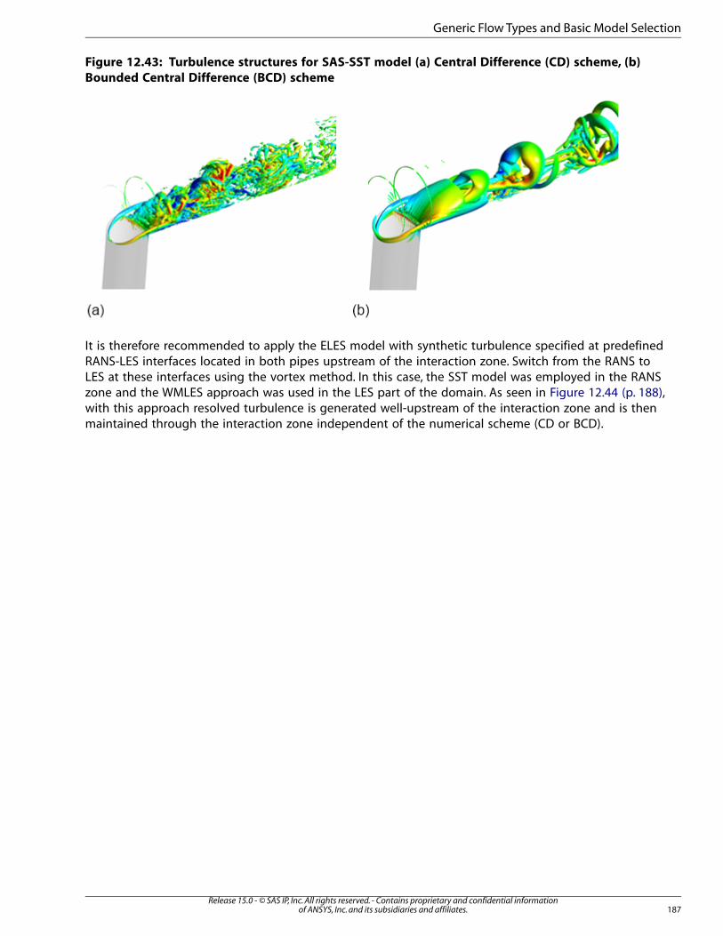
Figure 12.43: Turbulence structures for SAS-SST model (a) Central Difference (CD) scheme, (b)
Bounded Central Difference (BCD) scheme
It is therefore recommended to apply the ELES model with synthetic turbulence specified at predefinedRANS-LES interfaces located in both pipes upstream of the interaction zone. Switch from the RANS toLES at these interfaces using the vortex method. In this case, the SST model was employed in the RANSzone and the WMLES approach was used in the LES part of the domain. As seen in Figure 12.44 (p. 188),with this approach resolved turbulence is generated well-upstream of the interaction zone and is thenmaintained through the interaction zone independent of the numerical scheme (CD or BCD).
187Release 15.0 - © SAS IP, Inc. All rights reserved. - Contains proprietary and confidential information
of ANSYS, Inc. and its subsidiaries and affiliates.
Generic Flow Types and Basic Model Selection
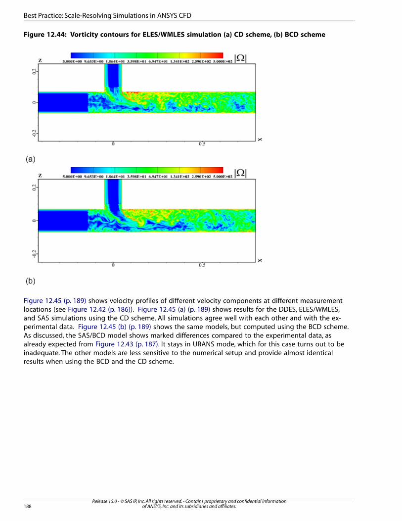
Figure 12.44: Vorticity contours for ELES/WMLES simulation (a) CD scheme, (b) BCD scheme
Figure 12.45 (p. 189) shows velocity profiles of different velocity components at different measurementlocations (see Figure 12.42 (p. 186)). Figure 12.45 (a) (p. 189) shows results for the DDES, ELES/WMLES,and SAS simulations using the CD scheme. All simulations agree well with each other and with the ex-perimental data. Figure 12.45 (b) (p. 189) shows the same models, but computed using the BCD scheme.As discussed, the SAS/BCD model shows marked differences compared to the experimental data, asalready expected from Figure 12.43 (p. 187). It stays in URANS mode, which for this case turns out to beinadequate. The other models are less sensitive to the numerical setup and provide almost identicalresults when using the BCD and the CD scheme.
Release 15.0 - © SAS IP, Inc. All rights reserved. - Contains proprietary and confidential informationof ANSYS, Inc. and its subsidiaries and affiliates.188
Best Practice: Scale-Resolving Simulations in ANSYS CFD
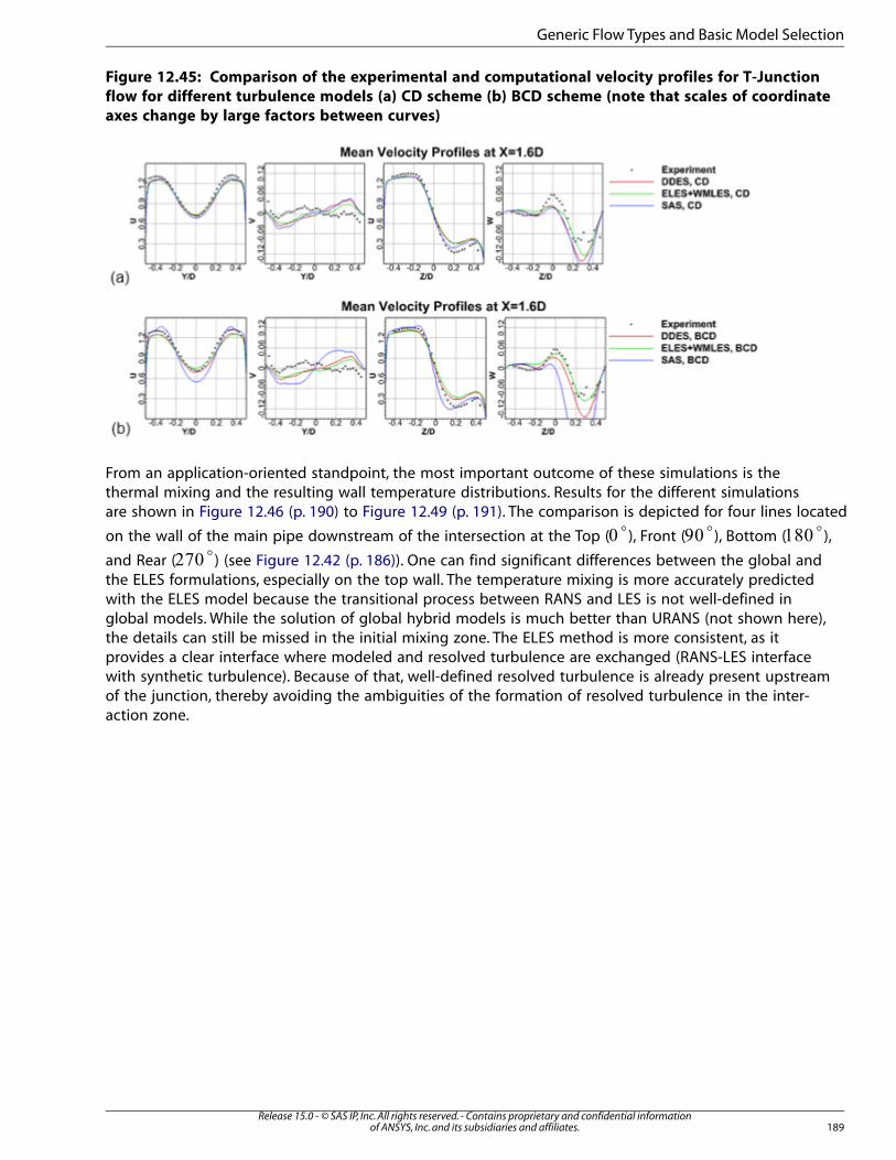
Figure 12.45: Comparison of the experimental and computational velocity profiles for T-Junction
flow for different turbulence models (a) CD scheme (b) BCD scheme (note that scales of coordinate
axes change by large factors between curves)
From an application-oriented standpoint, the most important outcome of these simulations is thethermal mixing and the resulting wall temperature distributions. Results for the different simulationsare shown in Figure 12.46 (p. 190) to Figure 12.49 (p. 191). The comparison is depicted for four lines located
on the wall of the main pipe downstream of the intersection at the Top (o
), Front (o
), Bottom (o
),
and Rear (o
) (see Figure 12.42 (p. 186)). One can find significant differences between the global andthe ELES formulations, especially on the top wall. The temperature mixing is more accurately predictedwith the ELES model because the transitional process between RANS and LES is not well-defined inglobal models. While the solution of global hybrid models is much better than URANS (not shown here),the details can still be missed in the initial mixing zone. The ELES method is more consistent, as itprovides a clear interface where modeled and resolved turbulence are exchanged (RANS-LES interfacewith synthetic turbulence). Because of that, well-defined resolved turbulence is already present upstreamof the junction, thereby avoiding the ambiguities of the formation of resolved turbulence in the inter-action zone.
189Release 15.0 - © SAS IP, Inc. All rights reserved. - Contains proprietary and confidential information
of ANSYS, Inc. and its subsidiaries and affiliates.
Generic Flow Types and Basic Model Selection
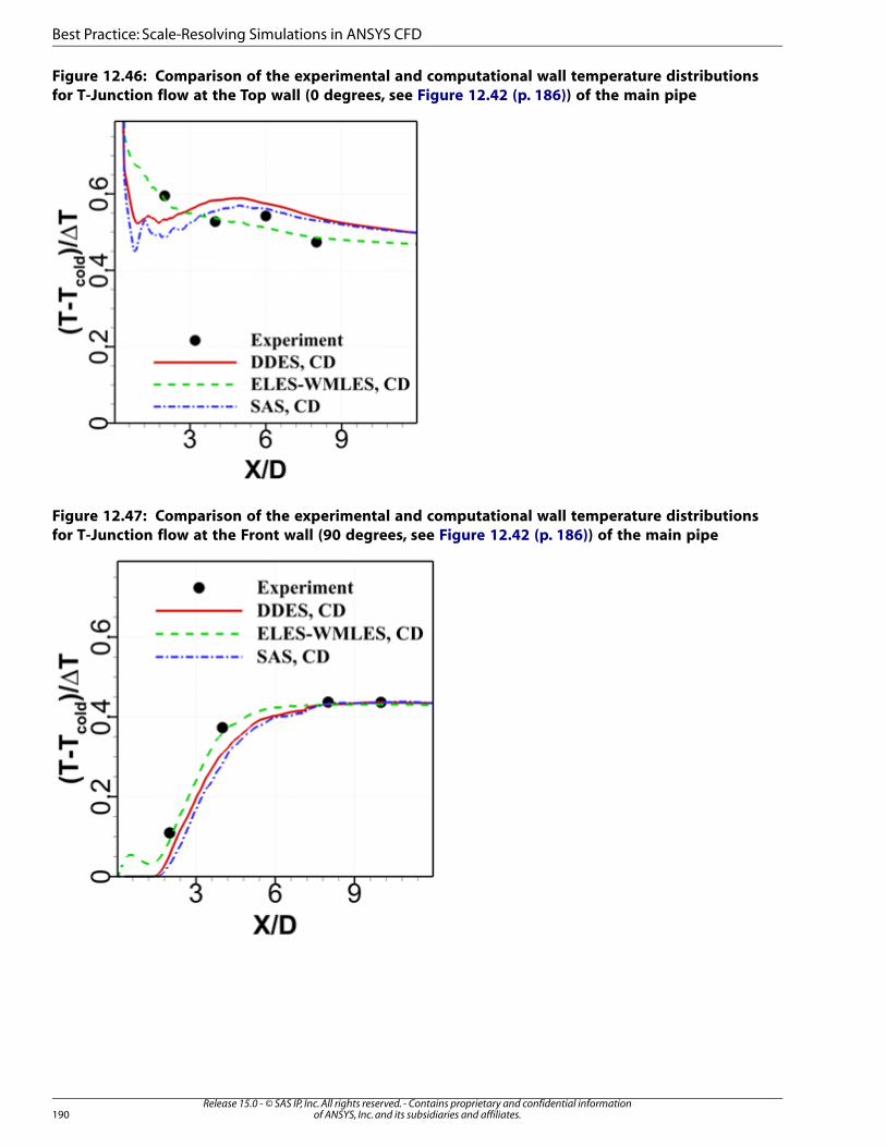
Figure 12.46: Comparison of the experimental and computational wall temperature distributions
for T-Junction flow at the Top wall (0 degrees, see Figure 12.42 (p. 186)) of the main pipe
Figure 12.47: Comparison of the experimental and computational wall temperature distributions
for T-Junction flow at the Front wall (90 degrees, see Figure 12.42 (p. 186)) of the main pipe
Release 15.0 - © SAS IP, Inc. All rights reserved. - Contains proprietary and confidential informationof ANSYS, Inc. and its subsidiaries and affiliates.190
Best Practice: Scale-Resolving Simulations in ANSYS CFD
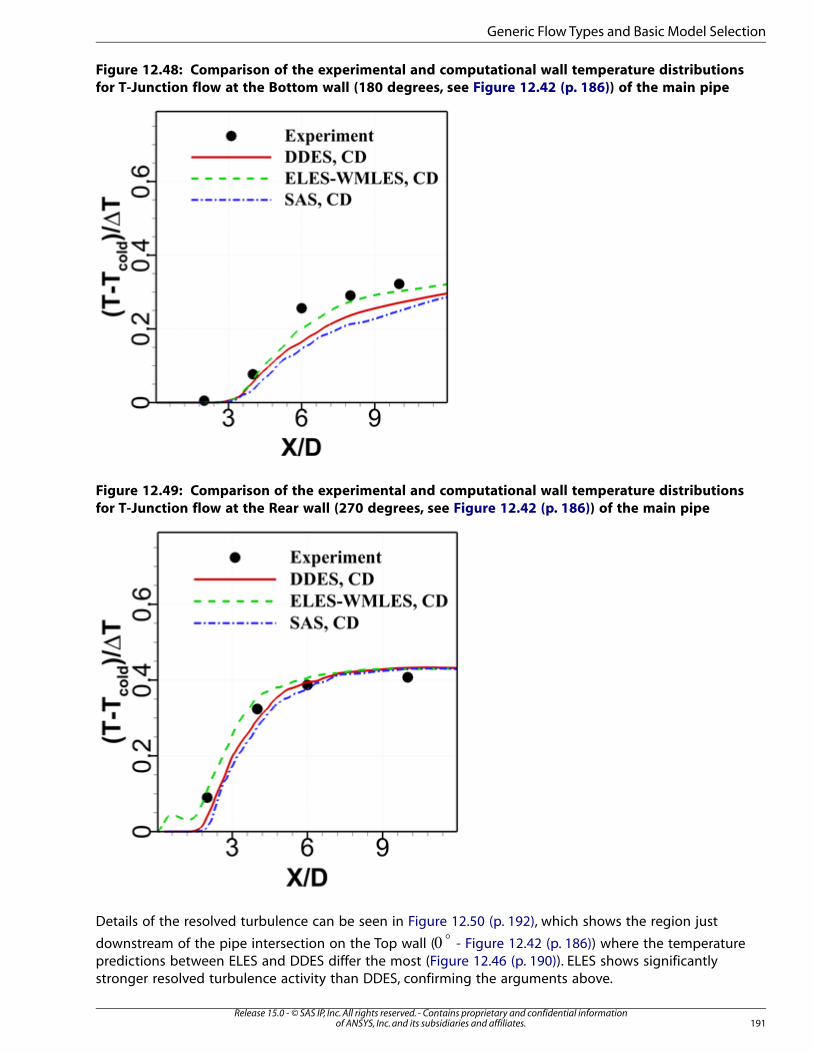
Figure 12.48: Comparison of the experimental and computational wall temperature distributions
for T-Junction flow at the Bottom wall (180 degrees, see Figure 12.42 (p. 186)) of the main pipe
Figure 12.49: Comparison of the experimental and computational wall temperature distributions
for T-Junction flow at the Rear wall (270 degrees, see Figure 12.42 (p. 186)) of the main pipe
Details of the resolved turbulence can be seen in Figure 12.50 (p. 192), which shows the region just
downstream of the pipe intersection on the Top wall (o
- Figure 12.42 (p. 186)) where the temperaturepredictions between ELES and DDES differ the most (Figure 12.46 (p. 190)). ELES shows significantlystronger resolved turbulence activity than DDES, confirming the arguments above.
191Release 15.0 - © SAS IP, Inc. All rights reserved. - Contains proprietary and confidential information
of ANSYS, Inc. and its subsidiaries and affiliates.
Generic Flow Types and Basic Model Selection

Figure 12.50: Comparison of turbulence structures on the Top wall downstream of the pipe
intersection (a) DDES model (b) ELES model
12.5. Numerical Settings for SRS
This chapter discusses:12.5.1. Spatial Discretization12.5.2. Pressure (ANSYS Fluent)12.5.3.Time Discretization
12.5.1. Spatial Discretization
12.5.1.1. Momentum
SRS models, as described in the previous section, serve the main purpose of dissipating the energy outof the turbulence spectrum at the limit of the grid resolution. The eddy viscosity is defined to providethe correct dissipation at the larger LES scales. This assumes that the numerical scheme is non-dissipativeand that all dissipation results from the LES model. For this reason, one is required to select a numericalscheme in the LES region with low dissipation, relative to the dissipation provided by a subgrid LESmodel. Another strategy is to avoid the introduction of the LES (subgrid) eddy viscosity and provide alldamping through the numerical scheme. This approach is called MILES (Monotone Integrated LargeEddy Simulation) (Boris et al., 1992 [1] (p. 207)). In ANSYS CFD, the standard LES methodology is followed,whereby the dissipation is introduced by a LES eddy viscosity model and the numerical dissipation iskept at a low value.
In order to achieve low numerical dissipation, you cannot use the standard numerical schemes forconvection that were developed for the RANS equations (Second Order Upwind Schemes, or SOU),which are dissipative by nature. In contrast, LES is carried out using Central Difference (CD) schemes.
Release 15.0 - © SAS IP, Inc. All rights reserved. - Contains proprietary and confidential informationof ANSYS, Inc. and its subsidiaries and affiliates.192
Best Practice: Scale-Resolving Simulations in ANSYS CFD
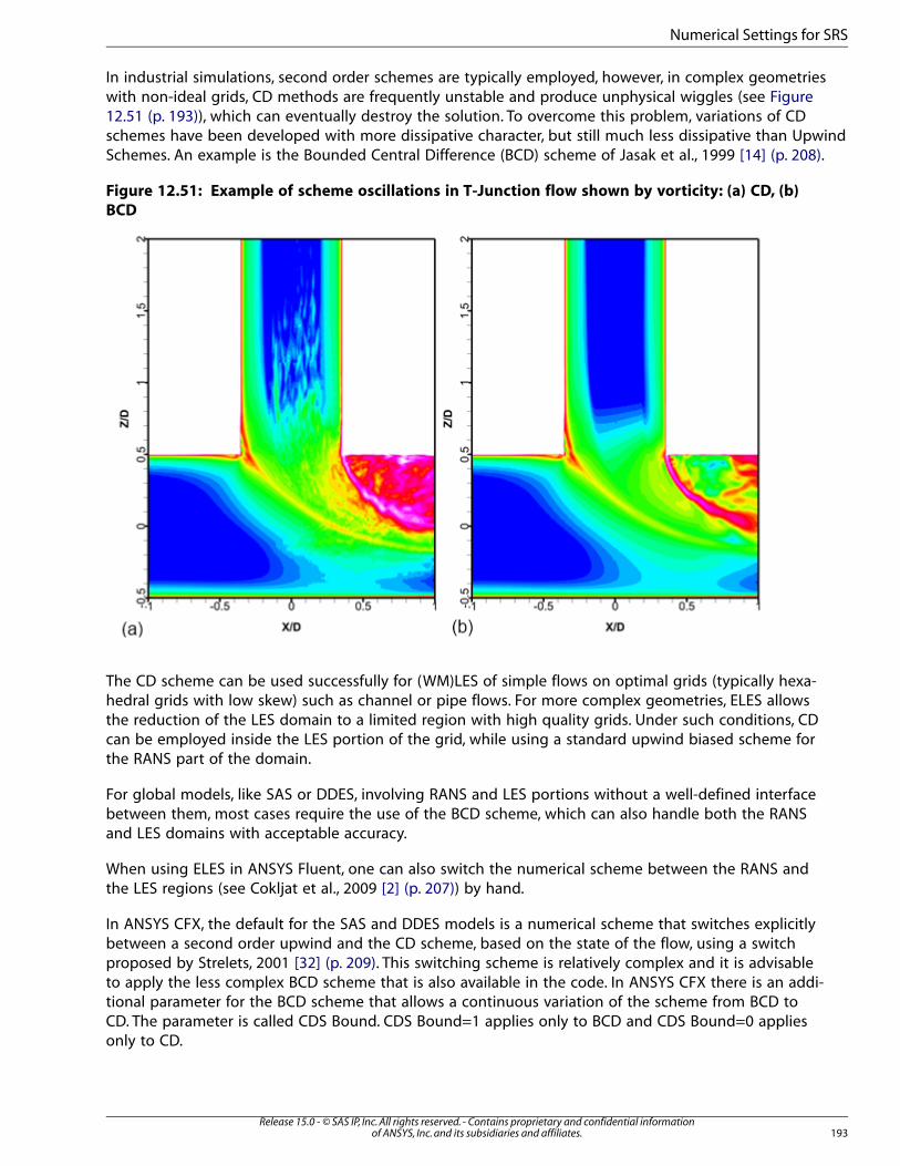
In industrial simulations, second order schemes are typically employed, however, in complex geometrieswith non-ideal grids, CD methods are frequently unstable and produce unphysical wiggles (see Figure12.51 (p. 193)), which can eventually destroy the solution. To overcome this problem, variations of CDschemes have been developed with more dissipative character, but still much less dissipative than UpwindSchemes. An example is the Bounded Central Difference (BCD) scheme of Jasak et al., 1999 [14] (p. 208).
Figure 12.51: Example of scheme oscillations in T-Junction flow shown by vorticity: (a) CD, (b)
BCD
The CD scheme can be used successfully for (WM)LES of simple flows on optimal grids (typically hexa-hedral grids with low skew) such as channel or pipe flows. For more complex geometries, ELES allowsthe reduction of the LES domain to a limited region with high quality grids. Under such conditions, CDcan be employed inside the LES portion of the grid, while using a standard upwind biased scheme forthe RANS part of the domain.
For global models, like SAS or DDES, involving RANS and LES portions without a well-defined interfacebetween them, most cases require the use of the BCD scheme, which can also handle both the RANSand LES domains with acceptable accuracy.
When using ELES in ANSYS Fluent, one can also switch the numerical scheme between the RANS andthe LES regions (see Cokljat et al., 2009 [2] (p. 207)) by hand.
In ANSYS CFX, the default for the SAS and DDES models is a numerical scheme that switches explicitlybetween a second order upwind and the CD scheme, based on the state of the flow, using a switchproposed by Strelets, 2001 [32] (p. 209). This switching scheme is relatively complex and it is advisableto apply the less complex BCD scheme that is also available in the code. In ANSYS CFX there is an addi-tional parameter for the BCD scheme that allows a continuous variation of the scheme from BCD toCD. The parameter is called CDS Bound. CDS Bound=1 applies only to BCD and CDS Bound=0 appliesonly to CD.
193Release 15.0 - © SAS IP, Inc. All rights reserved. - Contains proprietary and confidential information
of ANSYS, Inc. and its subsidiaries and affiliates.
Numerical Settings for SRS
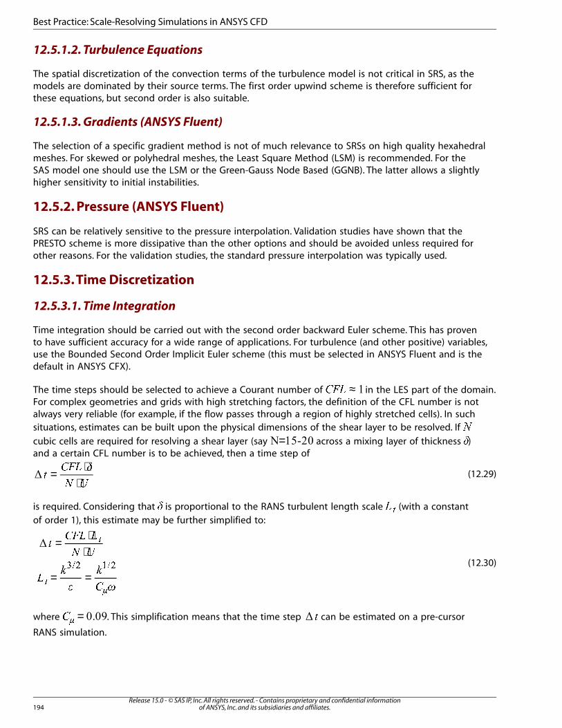
12.5.1.2. Turbulence Equations
The spatial discretization of the convection terms of the turbulence model is not critical in SRS, as themodels are dominated by their source terms. The first order upwind scheme is therefore sufficient forthese equations, but second order is also suitable.
12.5.1.3. Gradients (ANSYS Fluent)
The selection of a specific gradient method is not of much relevance to SRSs on high quality hexahedralmeshes. For skewed or polyhedral meshes, the Least Square Method (LSM) is recommended. For theSAS model one should use the LSM or the Green-Gauss Node Based (GGNB). The latter allows a slightlyhigher sensitivity to initial instabilities.
12.5.2. Pressure (ANSYS Fluent)
SRS can be relatively sensitive to the pressure interpolation. Validation studies have shown that thePRESTO scheme is more dissipative than the other options and should be avoided unless required forother reasons. For the validation studies, the standard pressure interpolation was typically used.
12.5.3. Time Discretization
12.5.3.1. Time Integration
Time integration should be carried out with the second order backward Euler scheme. This has provento have sufficient accuracy for a wide range of applications. For turbulence (and other positive) variables,use the Bounded Second Order Implicit Euler scheme (this must be selected in ANSYS Fluent and is thedefault in ANSYS CFX).
The time steps should be selected to achieve a Courant number of ≈��� in the LES part of the domain.For complex geometries and grids with high stretching factors, the definition of the CFL number is notalways very reliable (for example, if the flow passes through a region of highly stretched cells). In suchsituations, estimates can be built upon the physical dimensions of the shear layer to be resolved. If �
cubic cells are required for resolving a shear layer (say = across a mixing layer of thickness �)and a certain CFL number is to be achieved, then a time step of
(12.29)= ⋅⋅
����
�
is required. Considering that � is proportional to the RANS turbulent length scale � (with a constantof order 1), this estimate may be further simplified to:
(12.30)
= ⋅⋅
= =
���� �
� �
��
�
�
� �
�
��
��� ���
where =�� . This simplification means that the time step can be estimated on a pre-cursor
RANS simulation.
Release 15.0 - © SAS IP, Inc. All rights reserved. - Contains proprietary and confidential informationof ANSYS, Inc. and its subsidiaries and affiliates.194
Best Practice: Scale-Resolving Simulations in ANSYS CFD
You can also apply a more global estimate by assessing the through flow time, which is the time required
by a fluid element to pass through the LES domain of length � with velocity � : =� � ��� . With an
estimate of how many cells, � , will be passed along this trajectory, one obtains = ⋅� �� �� .
12.5.3.2. Time Advancement and Under-Relaxation (ANSYS Fluent)
There are several different settings for time advancement in ANSYS Fluent. The first choice is betweenthe Iterative (ITA) and the Non-Iterative Time Advancement (NITA). NITA should be checked for any newapplication as it can result in significant CPU savings. As a general guideline, NITA works well on highquality grids and for flows with limited additional physical coupling between the equations. WithinNITA, the fractional step scheme is recommended; however, one must be very cautious and conservativewith the assessment of the time step size. An attempt to perform a simulation with CFL>1 can lead toan incorrect solution. In addition, one should reduce residual tolerance for all equations to 0.0001.
For the ITA schemes (everything except NITA), the segregated solvers are typically faster than thecoupled solver. The optimal choice is in most cases the SIMPLEC scheme. The default under-relaxationparameters for this scheme are set for steady-state simulations. For SRS model simulations, they shouldbe changed to values as close as possible to 1 to improve iterative convergence. Typically, the numberof inner iteration loops ( ∼������ 10–20) required with SIMPLEC depends on the complexity of the flowproblem. The most critical quantity is the mass conservation. Mass residuals should decrease by at leastone order of magnitude every time step.
The coupled solver is slower per iteration, but it can lead to more robust convergence, and for complexcases can be advantageous. For the coupled solver, one would typically also specify under-relaxationvalues of (or close to) 1. The number of inner loops is typically ∼������ 5-10. In ANSYS CFX, the coupledsolver is used in all simulations.
For flows with additional physics (multiphase, combustion, and so on), the number of inner iterationsper time step can increase significantly for all solvers.
It is important to emphasize that the optimal under-relaxation factors and the optimal number of inneriterations is case-dependent. Some optimization might be required for achieving the most efficientresults.
12.6. Initial and Boundary Conditions
This chapter discusses:12.6.1. Initialization of SRS12.6.2. Boundary Conditions for SRS12.6.3. Symmetry vs. Periodicity
12.6.1. Initialization of SRS
In most cases it is best to initialize the SRS model using a RANS model solution. This recommendationis especially true for global hybrid RANS-LES models (SAS, DDES), which are based on an underlyingRANS model.
For pure LES or WMLES, ANSYS Fluent offers an option for initializing the flow by converting turbulencefrom RANS to LES mode (solve/initialize/init-instantaneous-vel ) using a syntheticturbulence generation routine. This option should be used with caution as it can, at times, have a det-rimental effect on the robustness of the simulation. It should be executed mainly for cases where nosynthetic turbulence is generated at an inlet/interface and where the inherent flow instability is not
195Release 15.0 - © SAS IP, Inc. All rights reserved. - Contains proprietary and confidential information
of ANSYS, Inc. and its subsidiaries and affiliates.
Initial and Boundary Conditions
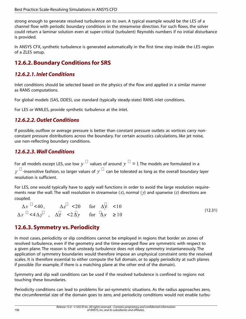
strong enough to generate resolved turbulence on its own. A typical example would be the LES of achannel flow with periodic boundary conditions in the streamwise direction. For such flows, the solvercould return a laminar solution even at super-critical (turbulent) Reynolds numbers if no initial disturbanceis provided.
In ANSYS CFX, synthetic turbulence is generated automatically in the first time step inside the LES regionof a ZLES setup.
12.6.2. Boundary Conditions for SRS
12.6.2.1. Inlet Conditions
Inlet conditions should be selected based on the physics of the flow and applied in a similar manneras RANS computations.
For global models (SAS, DDES), use standard (typically steady-state) RANS inlet conditions.
For LES or WMLES, provide synthetic turbulence at the inlet.
12.6.2.2. Outlet Conditions
If possible, outflow or average pressure is better than constant pressure outlets as vortices carry non-constant pressure distributions across the boundary. For certain acoustics calculations, like jet noise,use non-reflecting boundary conditions.
12.6.2.3. Wall Conditions
For all models except LES, use low +
� values of around =+� . The models are formulated in a
+� -insensitive fashion, so larger values of
+� can be tolerated as long as the overall boundary layer
resolution is sufficient.
For LES, one would typically have to apply wall functions in order to avoid the large resolution require-ments near the wall. The wall resolution in streamwise (�), normal (�) and spanwise (�) directions arecoupled.
(12.31)< < <
< < ≥
+ + +
+ + + + +� �
� �
12.6.3. Symmetry vs. Periodicity
In most cases, periodicity or slip conditions cannot be employed in regions that border on zones ofresolved turbulence, even if the geometry and the time-averaged flow are symmetric with respect toa given plane. The reason is that unsteady turbulence does not obey symmetry instantaneously. Theapplication of symmetry boundaries would therefore impose an unphysical constraint onto the resolvedscales. It is therefore essential to either compute the full domain, or to apply periodicity at such planesif possible (for example, if there is a matching plane at the other end of the domain).
Symmetry and slip wall conditions can be used if the resolved turbulence is confined to regions nottouching these boundaries.
Periodicity conditions can lead to problems for axi-symmetric situations. As the radius approaches zero,the circumferential size of the domain goes to zero, and periodicity conditions would not enable turbu-
Release 15.0 - © SAS IP, Inc. All rights reserved. - Contains proprietary and confidential informationof ANSYS, Inc. and its subsidiaries and affiliates.196
Best Practice: Scale-Resolving Simulations in ANSYS CFD
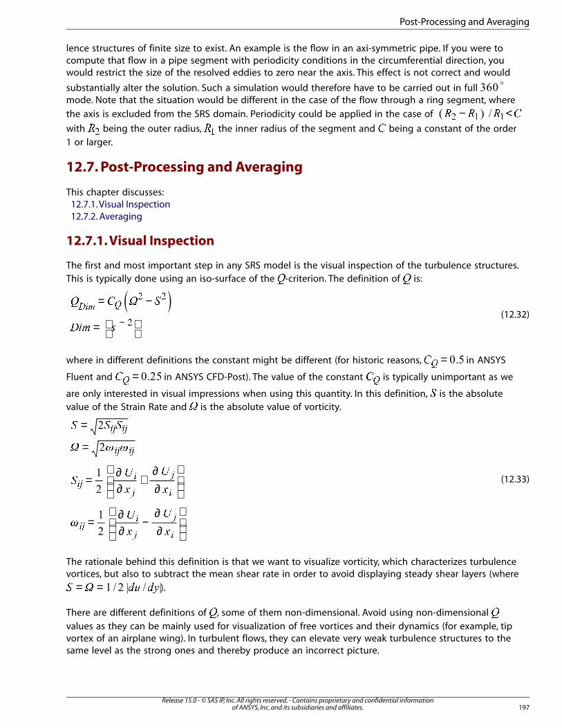
lence structures of finite size to exist. An example is the flow in an axi-symmetric pipe. If you were tocompute that flow in a pipe segment with periodicity conditions in the circumferential direction, youwould restrict the size of the resolved eddies to zero near the axis. This effect is not correct and would
substantially alter the solution. Such a simulation would therefore have to be carried out in full o
mode. Note that the situation would be different in the case of the flow through a ring segment, where
the axis is excluded from the SRS domain. Periodicity could be applied in the case of − <� � � �� � �
with �� being the outer radius, �� the inner radius of the segment and � being a constant of the order1 or larger.
12.7. Post-Processing and Averaging
This chapter discusses:12.7.1.Visual Inspection12.7.2. Averaging
12.7.1. Visual Inspection
The first and most important step in any SRS model is the visual inspection of the turbulence structures.This is typically done using an iso-surface of the -criterion. The definition of is:
(12.32)= −
=
−
� � �
��� �
��� �� �
�
where in different definitions the constant might be different (for historic reasons, =�� in ANSYS
Fluent and =�� in ANSYS CFD-Post). The value of the constant �� is typically unimportant as we
are only interested in visual impressions when using this quantity. In this definition, � is the absolutevalue of the Strain Rate and � is the absolute value of vorticity.
(12.33)
=
=
=
∂∂
+∂∂
=
∂∂
−∂∂
! " "
#
$
#
$
"#
$
#
$
%& %&
%& %&
%&%
&
&
%
%&%
&
&
%
The rationale behind this definition is that we want to visualize vorticity, which characterizes turbulencevortices, but also to subtract the mean shear rate in order to avoid displaying steady shear layers (where
= =' ( )* )+ ).
There are different definitions of ,, some of them non-dimensional. Avoid using non-dimensional -values as they can be mainly used for visualization of free vortices and their dynamics (for example, tipvortex of an airplane wing). In turbulent flows, they can elevate very weak turbulence structures to thesame level as the strong ones and thereby produce an incorrect picture.
197Release 15.0 - © SAS IP, Inc. All rights reserved. - Contains proprietary and confidential information
of ANSYS, Inc. and its subsidiaries and affiliates.
Post-Processing and Averaging
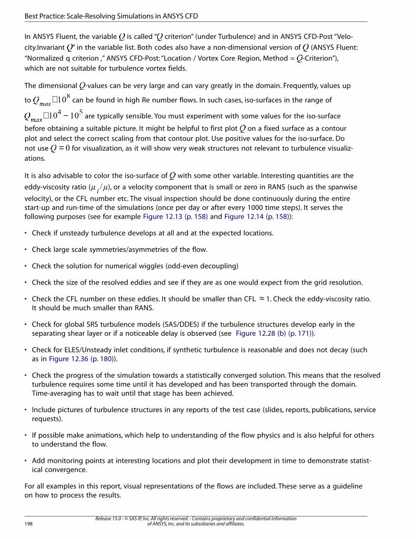
In ANSYS Fluent, the variable � is called “� criterion” (under Turbulence) and in ANSYS CFD-Post “Velo-
city.Invariant �” in the variable list. Both codes also have a non-dimensional version of � (ANSYS Fluent:
“Normalized q criterion ,” ANSYS CFD-Post: “Location / Vortex Core Region, Method = �-Criterion”),which are not suitable for turbulence vortex fields.
The dimensional �-values can be very large and can vary greatly in the domain. Frequently, values up
to ∼���
can be found in high Re number flows. In such cases, iso-surfaces in the range of
∼ −�� �
� � are typically sensible. You must experiment with some values for the iso-surface
before obtaining a suitable picture. It might be helpful to first plot � on a fixed surface as a contourplot and select the correct scaling from that contour plot. Use positive values for the iso-surface. Donot use =� for visualization, as it will show very weak structures not relevant to turbulence visualiz-ations.
It is also advisable to color the iso-surface of � with some other variable. Interesting quantities are the
eddy-viscosity ratio (� ��
), or a velocity component that is small or zero in RANS (such as the spanwise
velocity), or the CFL number etc. The visual inspection should be done continuously during the entirestart-up and run-time of the simulations (once per day or after every 1000 time steps). It serves thefollowing purposes (see for example Figure 12.13 (p. 158) and Figure 12.14 (p. 158)):
• Check if unsteady turbulence develops at all and at the expected locations.
• Check large scale symmetries/asymmetries of the flow.
• Check the solution for numerical wiggles (odd-even decoupling)
• Check the size of the resolved eddies and see if they are as one would expect from the grid resolution.
• Check the CFL number on these eddies. It should be smaller than CFL ≈ 1. Check the eddy-viscosity ratio.It should be much smaller than RANS.
• Check for global SRS turbulence models (SAS/DDES) if the turbulence structures develop early in theseparating shear layer or if a noticeable delay is observed (see Figure 12.28 (b) (p. 171)).
• Check for ELES/Unsteady inlet conditions, if synthetic turbulence is reasonable and does not decay (suchas in Figure 12.36 (p. 180)).
• Check the progress of the simulation towards a statistically converged solution. This means that the resolvedturbulence requires some time until it has developed and has been transported through the domain.Time-averaging has to wait until that stage has been achieved.
• Include pictures of turbulence structures in any reports of the test case (slides, reports, publications, servicerequests).
• If possible make animations, which help to understanding of the flow physics and is also helpful for othersto understand the flow.
• Add monitoring points at interesting locations and plot their development in time to demonstrate statist-ical convergence.
For all examples in this report, visual representations of the flows are included. These serve as a guidelineon how to process the results.
Release 15.0 - © SAS IP, Inc. All rights reserved. - Contains proprietary and confidential informationof ANSYS, Inc. and its subsidiaries and affiliates.198
Best Practice: Scale-Resolving Simulations in ANSYS CFD
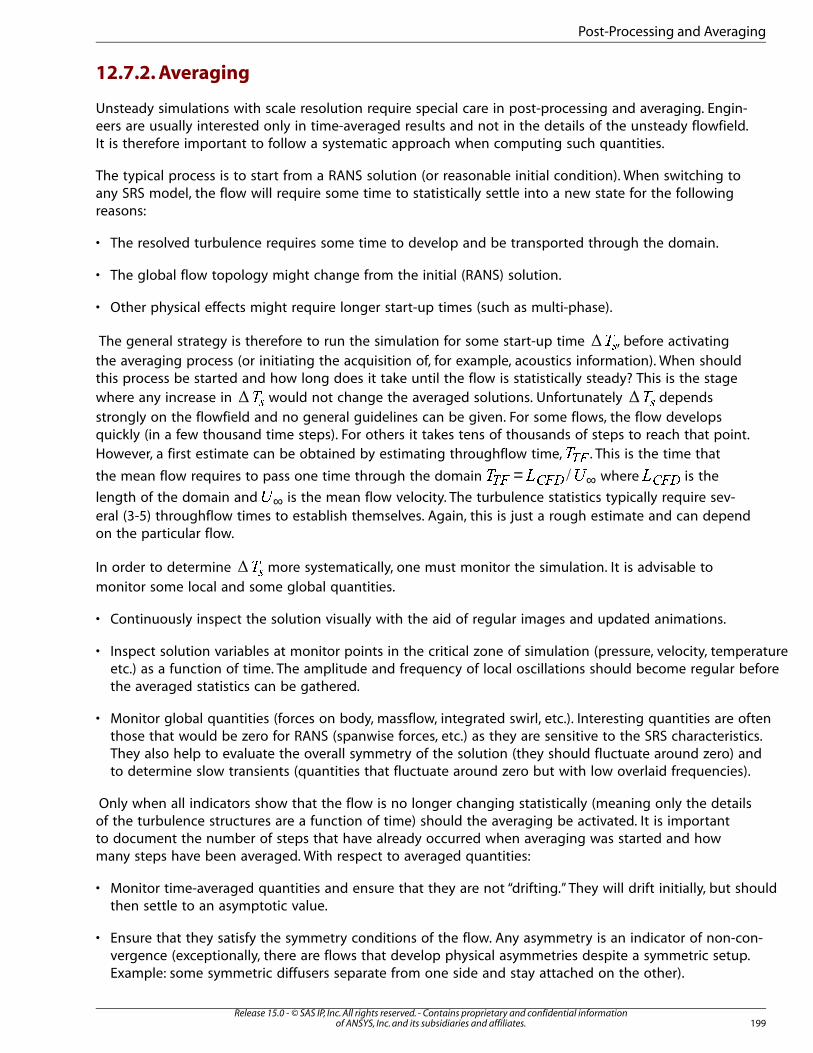
12.7.2. Averaging
Unsteady simulations with scale resolution require special care in post-processing and averaging. Engin-eers are usually interested only in time-averaged results and not in the details of the unsteady flowfield.It is therefore important to follow a systematic approach when computing such quantities.
The typical process is to start from a RANS solution (or reasonable initial condition). When switching toany SRS model, the flow will require some time to statistically settle into a new state for the followingreasons:
• The resolved turbulence requires some time to develop and be transported through the domain.
• The global flow topology might change from the initial (RANS) solution.
• Other physical effects might require longer start-up times (such as multi-phase).
The general strategy is therefore to run the simulation for some start-up time ��, before activatingthe averaging process (or initiating the acquisition of, for example, acoustics information). When shouldthis process be started and how long does it take until the flow is statistically steady? This is the stagewhere any increase in �� would not change the averaged solutions. Unfortunately �� dependsstrongly on the flowfield and no general guidelines can be given. For some flows, the flow developsquickly (in a few thousand time steps). For others it takes tens of thousands of steps to reach that point.However, a first estimate can be obtained by estimating throughflow time,��� . This is the time that
the mean flow requires to pass one time through the domain = ∞ �� � � where ���� is the
length of the domain and ∞� is the mean flow velocity. The turbulence statistics typically require sev-eral (3-5) throughflow times to establish themselves. Again, this is just a rough estimate and can dependon the particular flow.
In order to determine �� more systematically, one must monitor the simulation. It is advisable tomonitor some local and some global quantities.
• Continuously inspect the solution visually with the aid of regular images and updated animations.
• Inspect solution variables at monitor points in the critical zone of simulation (pressure, velocity, temperatureetc.) as a function of time. The amplitude and frequency of local oscillations should become regular beforethe averaged statistics can be gathered.
• Monitor global quantities (forces on body, massflow, integrated swirl, etc.). Interesting quantities are oftenthose that would be zero for RANS (spanwise forces, etc.) as they are sensitive to the SRS characteristics.They also help to evaluate the overall symmetry of the solution (they should fluctuate around zero) andto determine slow transients (quantities that fluctuate around zero but with low overlaid frequencies).
Only when all indicators show that the flow is no longer changing statistically (meaning only the detailsof the turbulence structures are a function of time) should the averaging be activated. It is importantto document the number of steps that have already occurred when averaging was started and howmany steps have been averaged. With respect to averaged quantities:
• Monitor time-averaged quantities and ensure that they are not “drifting.” They will drift initially, but shouldthen settle to an asymptotic value.
• Ensure that they satisfy the symmetry conditions of the flow. Any asymmetry is an indicator of non-con-vergence (exceptionally, there are flows that develop physical asymmetries despite a symmetric setup.Example: some symmetric diffusers separate from one side and stay attached on the other).
199Release 15.0 - © SAS IP, Inc. All rights reserved. - Contains proprietary and confidential information
of ANSYS, Inc. and its subsidiaries and affiliates.
Post-Processing and Averaging
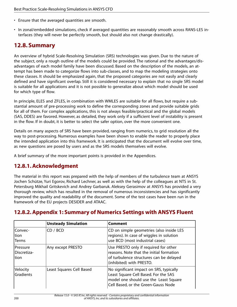
• Ensure that the averaged quantities are smooth.
• In zonal/embedded simulations, check if averaged quantities are reasonably smooth across RANS-LES in-terfaces (they will never be perfectly smooth, but should also not change drastically).
12.8. Summary
An overview of hybrid Scale-Resolving Simulation (SRS) technologies was given. Due to the nature ofthe subject, only a rough outline of the models could be provided. The rational and the advantages/dis-advantages of each model family have been discussed. Based on the description of the models, an at-tempt has been made to categorize flows into sub-classes, and to map the modeling strategies ontothese classes. It should be emphasized again, that the proposed categories are not easily and clearlydefined and have significant overlap. Still it is considered necessary to explain that no single SRS modelis suitable for all applications and it is not possible to generalize about which model should be usedfor which type of flow.
In principle, ELES and ZFLES, in combination with WMLES are suitable for all flows, but require a sub-stantial amount of pre-processing work to define the corresponding zones and provide suitable gridsfor all of them. For complex applications, this is not always feasible/practical and the global models(SAS, DDES) are favored. However, as detailed, they work only if a sufficient level of instability is presentin the flow. If in doubt, it is better to select the safer option, over the more convenient one.
Details on many aspects of SRS have been provided, ranging from numerics, to grid resolution all theway to post-processing. Numerous examples have been shown to enable the reader to properly placethe intended application into this framework. It is anticipated that the document will evolve over time,as new questions are posed by users and as the SRS models themselves will evolve.
A brief summary of the more important points is provided in the Appendices.
12.8.1. Acknowledgment
The material in this report was prepared with the help of members of the turbulence team at ANSYSJochen Schütze, Yuri Egorov, Richard Lechner, as well as with the help of the colleagues at NTS in St.Petersburg Mikhail Gritskevich and Andrey Garbaruk. Aleksey Gerasimov at ANSYS has provided a verythorough review, which has resulted in the removal of numerous inconsistencies and has significantlyimproved the quality and readability of the document. Some of the test cases have been run in theframework of the EU projects DESIDER and ATAAC.
12.8.2. Appendix 1: Summary of Numerics Settings with ANSYS Fluent
CommentUnsteady Simulation
CD on simple geometries (also inside LESregions). In case of wiggles in solutionuse BCD (most industrial cases)
CD / BCDConvec-tionTerms
Use PRESTO only if required for otherreasons. Note that the initial formation
Any except PRESTOPressureDiscretiza-tion of turbulence structures can be delayed
(inhibited) with PRESTO.
No significant impact on SRS, typicallyLeast Square Cell Based. For the SAS
Least Squares Cell BasedVelocityGradients
model one should use the Least SquareCell Based, or the Green-Gauss Node
Release 15.0 - © SAS IP, Inc. All rights reserved. - Contains proprietary and confidential informationof ANSYS, Inc. and its subsidiaries and affiliates.200
Best Practice: Scale-Resolving Simulations in ANSYS CFD
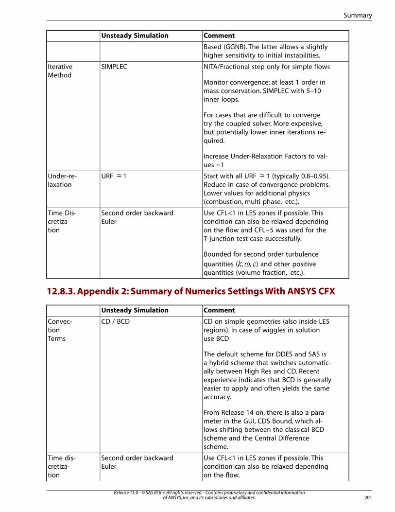
CommentUnsteady Simulation
Based (GGNB). The latter allows a slightlyhigher sensitivity to initial instabilities.
NITA/Fractional step only for simple flowsSIMPLECIterativeMethod
Monitor convergence: at least 1 order inmass conservation. SIMPLEC with 5–10inner loops.
For cases that are difficult to convergetry the coupled solver. More expensive,but potentially lower inner iterations re-quired.
Increase Under-Relaxation Factors to val-ues ~1
Start with all URF ≈ 1 (typically 0.8–0.95).Reduce in case of convergence problems.
URF ≈ 1Under-re-laxation
Lower values for additional physics(combustion, multi phase, etc.).
Use CFL<1 in LES zones if possible. Thiscondition can also be relaxed depending
Second order backwardEuler
Time Dis-cretiza-tion on the flow and CFL~5 was used for the
T-junction test case successfully.
Bounded for second order turbulence
quantities (�,�, �) and other positivequantities (volume fraction, etc.).
12.8.3. Appendix 2: Summary of Numerics Settings With ANSYS CFX
CommentUnsteady Simulation
CD on simple geometries (also inside LESregions). In case of wiggles in solutionuse BCD
CD / BCDConvec-tionTerms
The default scheme for DDES and SAS isa hybrid scheme that switches automatic-ally between High Res and CD. Recentexperience indicates that BCD is generallyeasier to apply and often yields the sameaccuracy.
From Release 14 on, there is also a para-meter in the GUI, CDS Bound, which al-lows shifting between the classical BCDscheme and the Central Differencescheme.
Use CFL<1 in LES zones if possible. Thiscondition can also be relaxed dependingon the flow.
Second order backwardEuler
Time dis-cretiza-tion
201Release 15.0 - © SAS IP, Inc. All rights reserved. - Contains proprietary and confidential information
of ANSYS, Inc. and its subsidiaries and affiliates.
Summary
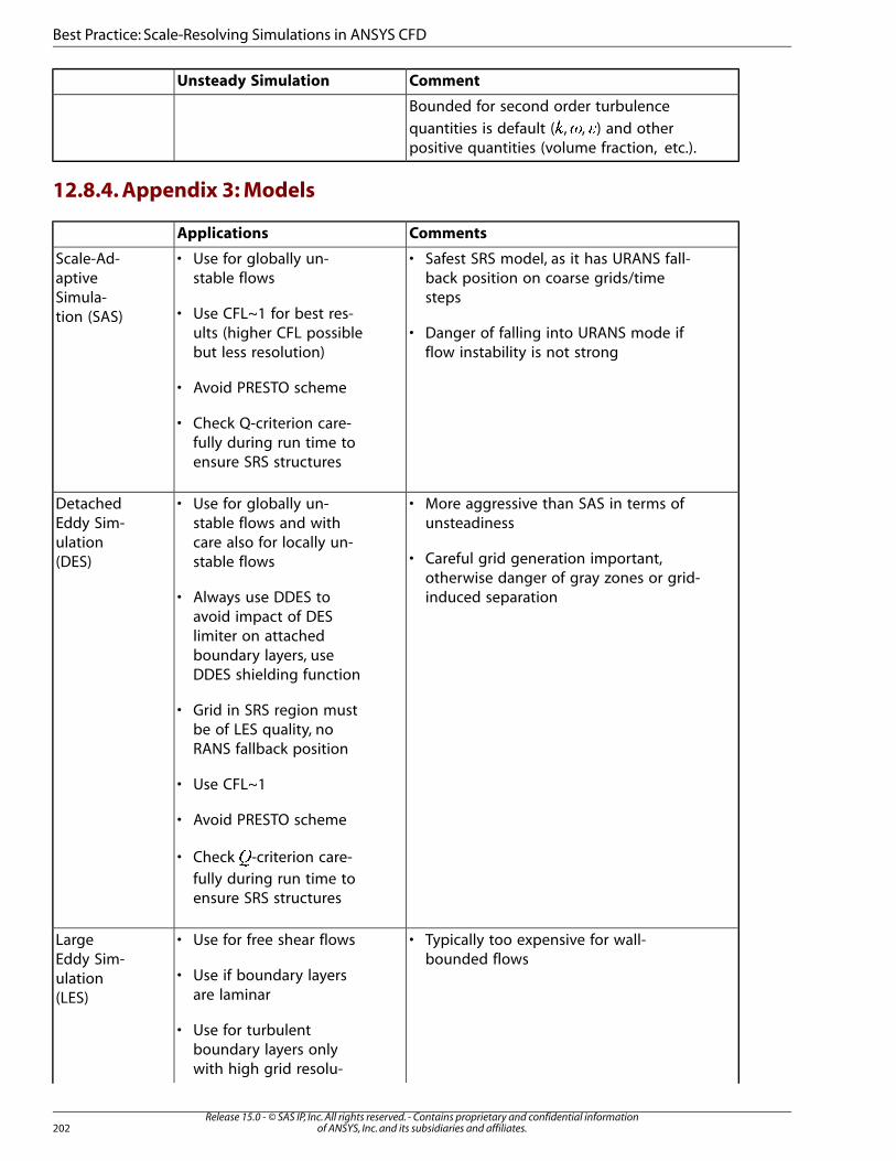
CommentUnsteady Simulation
Bounded for second order turbulence
quantities is default (�,�, �) and otherpositive quantities (volume fraction, etc.).
12.8.4. Appendix 3: Models
CommentsApplications
Scale-Ad-aptive
• Safest SRS model, as it has URANS fall-back position on coarse grids/timesteps
• Use for globally un-stable flows
Simula-tion (SAS) • Use CFL~1 for best res-
ults (higher CFL possiblebut less resolution)
• Danger of falling into URANS mode ifflow instability is not strong
• Avoid PRESTO scheme
• Check Q-criterion care-fully during run time toensure SRS structures
DetachedEddy Sim-
• More aggressive than SAS in terms ofunsteadiness
• Use for globally un-stable flows and withcare also for locally un-stable flows
ulation(DES) • Careful grid generation important,
otherwise danger of gray zones or grid-induced separation• Always use DDES to
avoid impact of DESlimiter on attachedboundary layers, useDDES shielding function
• Grid in SRS region mustbe of LES quality, noRANS fallback position
• Use CFL~1
• Avoid PRESTO scheme
• Check �-criterion care-fully during run time toensure SRS structures
LargeEddy Sim-
•• Use for free shear flows Typically too expensive for wall-bounded flows
• Use if boundary layersare laminar
ulation(LES)
• Use for turbulentboundary layers onlywith high grid resolu-
Release 15.0 - © SAS IP, Inc. All rights reserved. - Contains proprietary and confidential informationof ANSYS, Inc. and its subsidiaries and affiliates.202
Best Practice: Scale-Resolving Simulations in ANSYS CFD
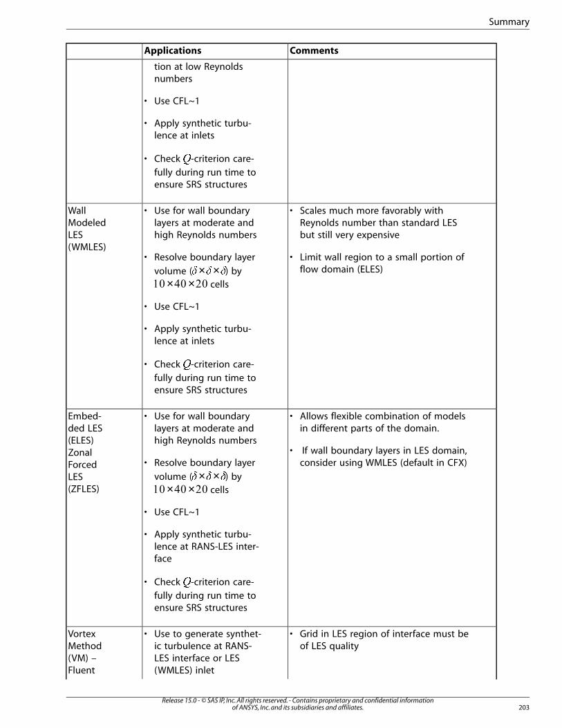
CommentsApplications
tion at low Reynoldsnumbers
• Use CFL~1
• Apply synthetic turbu-lence at inlets
• Check �-criterion care-fully during run time toensure SRS structures
WallModeled
• Scales much more favorably withReynolds number than standard LESbut still very expensive
• Use for wall boundarylayers at moderate andhigh Reynolds numbersLES
(WMLES)•• Limit wall region to a small portion of
flow domain (ELES)Resolve boundary layer
volume ( × ×� � �) by× × cells
• Use CFL~1
• Apply synthetic turbu-lence at inlets
• Check �-criterion care-fully during run time toensure SRS structures
Embed-ded LES
• Allows flexible combination of modelsin different parts of the domain.
• Use for wall boundarylayers at moderate andhigh Reynolds numbers(ELES)
Zonal • If wall boundary layers in LES domain,consider using WMLES (default in CFX)• Resolve boundary layer
volume ( × ×� � �) by× × cells
ForcedLES(ZFLES)
• Use CFL~1
• Apply synthetic turbu-lence at RANS-LES inter-face
• Check �-criterion care-fully during run time toensure SRS structures
VortexMethod
•• Use to generate synthet-ic turbulence at RANS-
Grid in LES region of interface must beof LES quality
(VM) –Fluent
LES interface or LES(WMLES) inlet
203Release 15.0 - © SAS IP, Inc. All rights reserved. - Contains proprietary and confidential information
of ANSYS, Inc. and its subsidiaries and affiliates.
Summary
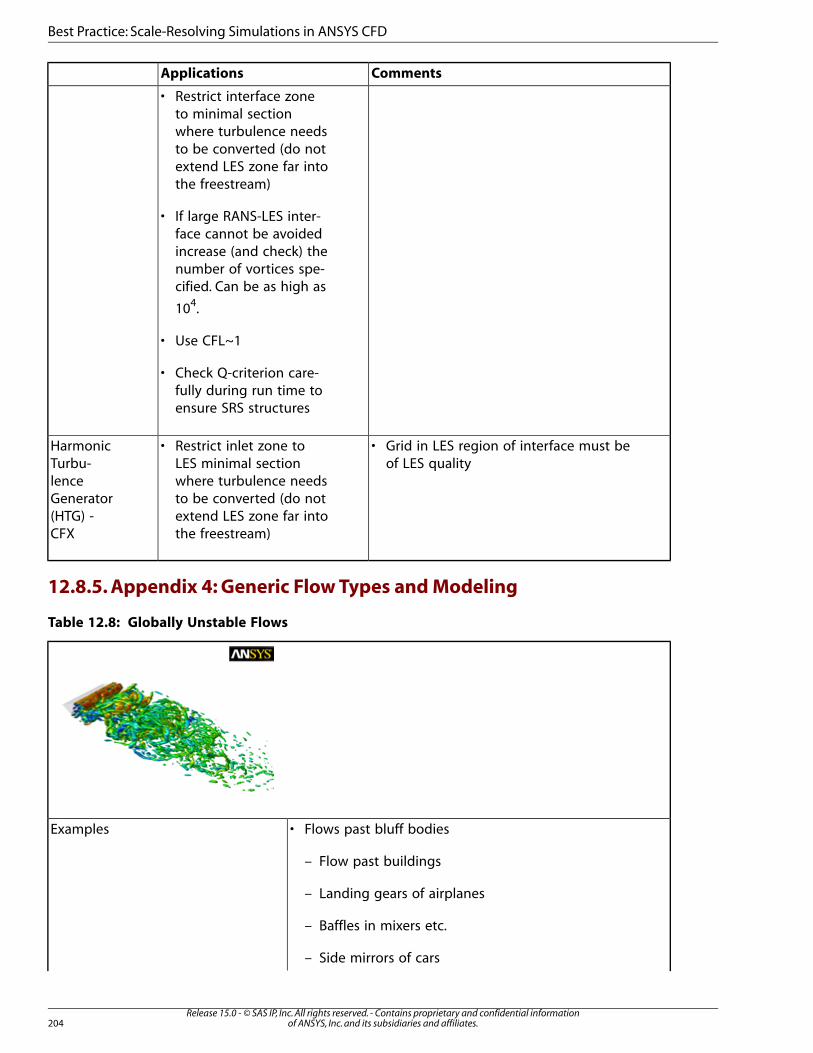
CommentsApplications
• Restrict interface zoneto minimal sectionwhere turbulence needsto be converted (do notextend LES zone far intothe freestream)
• If large RANS-LES inter-face cannot be avoidedincrease (and check) thenumber of vortices spe-cified. Can be as high as
104.
• Use CFL~1
• Check Q-criterion care-fully during run time toensure SRS structures
HarmonicTurbu-
•• Grid in LES region of interface must beof LES quality
Restrict inlet zone toLES minimal sectionwhere turbulence needslenceto be converted (do notGeneratorextend LES zone far intothe freestream)
(HTG) -CFX
12.8.5. Appendix 4: Generic Flow Types and Modeling
Table 12.8: Globally Unstable Flows
Examples • Flows past bluff bodies
– Flow past buildings
– Landing gears of airplanes
– Baffles in mixers etc.
– Side mirrors of cars
Release 15.0 - © SAS IP, Inc. All rights reserved. - Contains proprietary and confidential informationof ANSYS, Inc. and its subsidiaries and affiliates.204
Best Practice: Scale-Resolving Simulations in ANSYS CFD
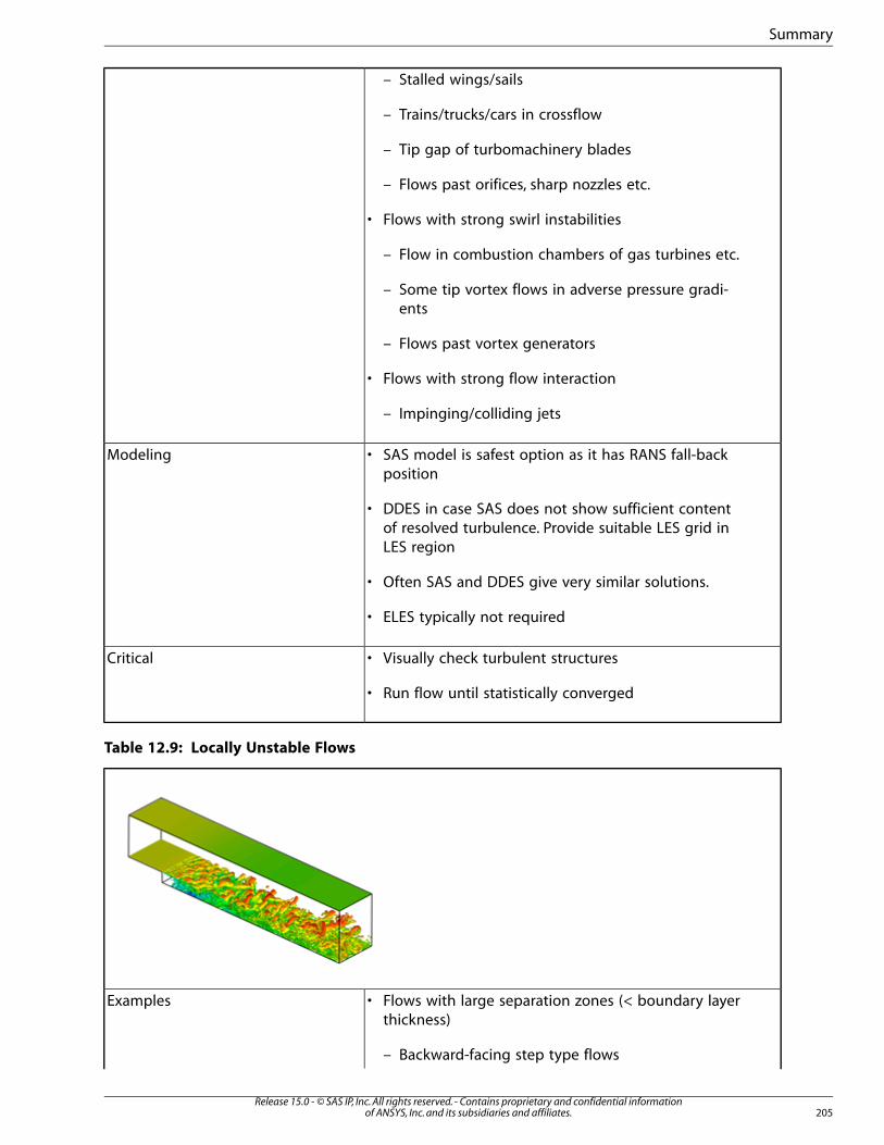
– Stalled wings/sails
– Trains/trucks/cars in crossflow
– Tip gap of turbomachinery blades
– Flows past orifices, sharp nozzles etc.
• Flows with strong swirl instabilities
– Flow in combustion chambers of gas turbines etc.
– Some tip vortex flows in adverse pressure gradi-ents
– Flows past vortex generators
• Flows with strong flow interaction
– Impinging/colliding jets
Modeling • SAS model is safest option as it has RANS fall-backposition
• DDES in case SAS does not show sufficient contentof resolved turbulence. Provide suitable LES grid inLES region
• Often SAS and DDES give very similar solutions.
• ELES typically not required
Critical • Visually check turbulent structures
• Run flow until statistically converged
Table 12.9: Locally Unstable Flows
Examples • Flows with large separation zones (< boundary layerthickness)
– Backward-facing step type flows
205Release 15.0 - © SAS IP, Inc. All rights reserved. - Contains proprietary and confidential information
of ANSYS, Inc. and its subsidiaries and affiliates.
Summary
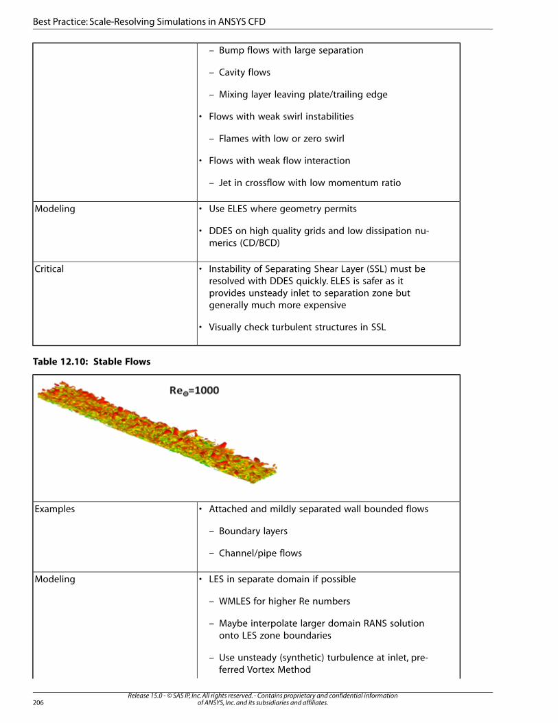
– Bump flows with large separation
– Cavity flows
– Mixing layer leaving plate/trailing edge
• Flows with weak swirl instabilities
– Flames with low or zero swirl
• Flows with weak flow interaction
– Jet in crossflow with low momentum ratio
Modeling • Use ELES where geometry permits
• DDES on high quality grids and low dissipation nu-merics (CD/BCD)
Critical • Instability of Separating Shear Layer (SSL) must beresolved with DDES quickly. ELES is safer as itprovides unsteady inlet to separation zone butgenerally much more expensive
• Visually check turbulent structures in SSL
Table 12.10: Stable Flows
Examples • Attached and mildly separated wall bounded flows
– Boundary layers
– Channel/pipe flows
Modeling • LES in separate domain if possible
– WMLES for higher Re numbers
– Maybe interpolate larger domain RANS solutiononto LES zone boundaries
– Use unsteady (synthetic) turbulence at inlet, pre-ferred Vortex Method
Release 15.0 - © SAS IP, Inc. All rights reserved. - Contains proprietary and confidential informationof ANSYS, Inc. and its subsidiaries and affiliates.206
Best Practice: Scale-Resolving Simulations in ANSYS CFD
• ELES in combined RANS-LES simulation
– Define LES zone as detailed in Sec-tion 12.4.3 (p. 171). Extend LES zone to leave spacearound critical area.
– Place RANS-LES interface into region of uncriticalflows (equilibrium boundary layers etc.)
Critical • Visually check turbulent structures
• Provide sufficient grid resolution in (WM)LES zonesespecially for wall-bounded flows (Sec-tion 12.4.3.3 (p. 172)).
• CFL number<1.
12.9. Scale-Resolving Simulations References
[1] Boris, J. P., Grinstein, F. F., Oran, E. S., and Kolbe, R. S. “New insights into Large Eddy Simulation”. Fluid
Dynamic Research. Vol. 10. 199-228. 1992.
[2] Cokljat D., Caradi D., Link G., Lechner R., and Menter F.R. “Embedded LES Methodology for General-
Purpose CFD Solvers”. 22-24 June 2009. Proc. Turbulent Shear Flow Phenomena, 6th Int. Symp.Turbulence and Shear Flow Phenomena. Seoul, Korea. . 1191-1196.
[3] Comte-Bellot, G., and Corrsin, S. “Simple Eulerian time correlation of full- and narrow-band velocity
signals in grid-generated, “isotropic” turbulence”. Journal of Fluid Mechanics. Vol. 48, Part 2. 273-337. 1971.
[4] Davidson, L. “Evaluation of the SAS-SST Model Channel Flow, Asymmetric Diffuser and Axi-Symmetric
Hill”. Proceedings European Conference on Computational Fluid Dynamics . ECCOMAS CFD. .2006.
[5] Durbin, P., and Pettersson Reif, B.A. Statistical theory of turbulent flows. John Wiley and Sons, Ltd. UK.2003.
[6] Egorov Y., Menter F.R., and Cokljat D. “Scale-Adaptive Simulation Method for Unsteady Flow Predictions.
Part 2: Application to Aerodynamic Flow”. Flow Turbulence and Combustion. Vol. 85, No. 1. 139-165. 2010.
[7] Fröhlich J., Mellen C.P., Rodi W., Temmerman L., and Leschziner M. “Highly resolved large-eddy simu-
lation of separated flow in a channel with streamwise periodic constrictions”. Journal of Fluid
Mechanics. Vol. 526. 19–66. 2005.
[8] Fröhlich J., and von Terzi, D. “Hybrid LES/RANS methods for simulation of turbulent flows”. Progress in
Aerospace Sciences. Vol. 44, Issue 5. 349-377. 2008.
[9] Girimaji, S. S. “Partially-Averaged Navier-Stokes Method: A RANS to DNS Bridging Method”. 2004.
207Release 15.0 - © SAS IP, Inc. All rights reserved. - Contains proprietary and confidential information
of ANSYS, Inc. and its subsidiaries and affiliates.
Scale-Resolving Simulations References
[10] Girimaji, S., and Abdul-Hamid, K.S. “Partially-averaged Navier-Stokes model for turbulence: implement-
ation and validation”. AIAA Aerospace Sciences Meeting and Exhibit. Reno, Nevada. . 2005-0502.2005.
[11] Gritskevich, M.S. Garbaruk, A.V., Schütze, J., and Menter F.R. “Sensitization of DDES and IDDES Formu-
lations to the −� � Shear-Stress Transport Model”. Flow Turbulence and Combustion. 2012.
[12] Guerts, J. B. Elements of direct and large-eddy simulation. Edwards Inc. Philadelphia, USA. 2004.
[13] Hanjalic, K., and Launder, B. Modelling Turbulence in Engineering and the Environment. CambridgeUniversity Press. Cambridge, UK. 2011.
[14] Jasak H., Weller H.G., and Gosman A.D. “High Resolution Differencing Scheme for Arbitrarily Unstructured
Meshes”. International Journal for Numerical Methods in Fluids. Vol. 31. 431-449. 1999.
[15] Mathey, F., Cokljat, D., Bertoglio, J.P., and Sergent, E. “Specification of LES Inlet Boundary Condition
Using Vortex Method. 4th International Symposium on Turbulence, Heat and Mass Transfer. An-talya, Turkey. . 2003.
[16] Menter, F. R. “Two-equation eddy-viscosity turbulence models for engineering applications”. AIAA
Journal. Vol. 32, No. 8. 1598–1605. 1994.
[17] Menter F.R., Garbaruk A., and Smirnov P. “Scale adaptive simulation with artificial forcing”. Proc. 3rdSymposium on Hybrid RANS-LES Methods . . 2009.
[18] Menter, F.R., and Egorov, Y. “Scale-Adaptive Simulation Method for Unsteady Flow Predictions. Part 1:
Theory and Model Description”. Flow, Turbulence and Combustion . Vol. 85, No. 1. 113– 138. 2010.
[19] Menter, F.R., and Kuntz, M. “Adaptation of Eddy-Viscosity Turbulence Models to Unsteady Separated
Flow Behind Vehicles”. Proc. Conf. The Aerodynamics of Heavy Vehicles: Trucks, Busses and Trains.Asilomar, California. Springer . . 2002.
[20] Michelassi V., Wissink, J. G., and Rodi W. “Direct numerical simulation, large eddy simulation and un-
steady Reynolds-averaged Navier-Stokes simulations of periodic unsteady flow in a low-pressure
turbine cascade: A comparison”. Journal of Power and Engineering . Vol 217, Number 4. 403– 411.2003.
[21] Nicoud, F., and Ducros, F. “Subgrid-scale stress modelling based on the square of the velocity gradient
tensor”. Flow, Turbulence and Combustion . Vol. 62. 183– 200. 1999.
[22] Reichardt, H. “Vollstandige Darstellung der turbulenten Geschwindigkeitsverteilung in glatten Leitungen”.Zeitschrift fur Angewandte Mathematik und Mechanik . Vol. 31. 208– 219. 1951.
[23] Rotta, J.C. “Turbulente Strömumgen”. BG Teubner Stuttgart. 1972.
[24] Sagaut, P., Deck, S., and Terracol, M. Multiscale and multiresolution approaches in turbulence. Imper-ial College Press. London. 2006.
[25] Schildmacher, K.-U., Koch, R., Wittig, S., Krebs, W., and Hoffmann, S. “Experimental investigations of
the temporal air-fuel mixing fluctuations and cold flow instabilities of a premixing gas turbine
burner”. ASME Paper 2000-GT-0084. 2000.
[26] Shur, M.L., Spalart, P.R., Strelets, M.K., and Travin, A.K. “A hybrid RANS-LES approach with delayed-DES
and wall-modeled LES capabilities”. International Journal of Heat and Fluid Flow . Vol. 29. 1638-1649. 2008.
Release 15.0 - © SAS IP, Inc. All rights reserved. - Contains proprietary and confidential informationof ANSYS, Inc. and its subsidiaries and affiliates.208
Best Practice: Scale-Resolving Simulations in ANSYS CFD
[27] Sjunnesson, A., Henriksson, R., and Lofstrom, C. “CARS measurements and Visualization of Reacting
Flows in Bluff Body Stabilized Flame”. AIAA Paper 1992–3650. 1992.
[28] Smagorinsky, J. “General Circulation Experiments with the Primitive Equations”. Monthly Weather Review.Vol. 91. 99 – 165. 1963.
[29] Spalart, P.R., Jou, W., Strelets, M., and Allmaras, S. “Comments on the feasibility of LES for wings, and
on a hybrid RANS/LES approach”. Advances in DNS/LES. 1st AFOSR Int. Conf. on DNS/LES. . 1997.
[30] Spalart, P. R. “Strategies for turbulence modelling and simulations”. International Journal of Heat and
Fluid Flow. Vol. 21. 2. 2000.
[31] Spalart, P., Deck, S., Shur, M., Squires, K., Strelets, M., and Travin, A. “A New Version of Detached Eddy
Simulation, Resistant to Ambiguous Grid Densities”. Journal of Theoretical and Computational Fluid
Dynamics. Vol. 20. 181 –195. 2006.
[32] Strelets, M. “Detached Eddy Simulation of massively separated flows”. AIAA Paper 2001-879. 2001.
[33] Travin, A., Sur M., Strelets, M., and Spalart P. “Physical and numerical upgrades in the detached eddy
simulation of complex turbulent flows , In Advances in LES of complex flows ”. eds. R. Friedrich, W.Rodi . Kluwer Acad. New York. 239-254. 2000.
[34] Vogel, J.C., and Eaton, J.K. “Combined heat transfer and fluid dynamic measurements downstream of
a backward-facing step”. Journal of Heat and Mass Transfer. Vol. 107. 922 –929. 1985.
[35] Wagner, C., Hüttl, T., and Sagaut, P. “Large-eddy simulation for acoustics”. Cambridge University Press.2007.
[36] Westin, J., Alavyoon F., Andersson, L. Veber, P., Henriksson, M., and Andersson, C. “Experiments and
Unsteady CFD-Calculations of Thermal Mixing in a T-Junction” . OECD/NEA/IAEA Workshop on theBenchmarking of CFD Codes for Application to Nuclear Reactor Safety (CFD4NRS). Munich, Ger-many. . 1–15. 2006.
[37] Widenhorn, A., Noll, B., and Aigner, M. “Numerical Study of a Non-Reacting Turbulent Flow in a Turbine
Model Combustor”. AIAA Paper 2009-647, Orlando Florida . 2009.
[38] Wilcox, D.C. “Turbulence Modeling for CFD”. DCW Industries Inc. 3rd Edition. 2006.
209Release 15.0 - © SAS IP, Inc. All rights reserved. - Contains proprietary and confidential information
of ANSYS, Inc. and its subsidiaries and affiliates.
Scale-Resolving Simulations References

Release 15.0 - © SAS IP, Inc. All rights reserved. - Contains proprietary and confidential informationof ANSYS, Inc. and its subsidiaries and affiliates.210
Chapter 13: CFX Command Language (CCL)
The CFX Command Language (CCL) is the internal communication and command language of ANSYSCFX. It is a simple language that can be used to create objects or perform actions in the post-processor.All CCL statements can be classified into one of three categories:
• Object and parameter definitions, which are described in Object Creation and Deletion.
• CCL actions, which are commands that perform a specific task (such as reading a session file) and whichare described in Command Actions in the CFD-Post User's Guide.
• Power Syntax programming, which uses the Perl programming language to allow loops, logic, and custommacros (subroutines). Power Syntax enables you to embed Perl commands into CCL to achieve powerfulquantitative post-processing. For details, see Power Syntax in ANSYS CFX (p. 307).
State files and session files contain object definitions in CCL. In addition, session files can also containCCL action commands. You can view and modify the CCL in these files by using a text editor.
For more information, see Object Creation and Deletion.
13.1. CFX Command Language (CCL) Syntax
The following topics will be discussed:
• Basic Terminology (p. 212)
• The Data Hierarchy (p. 212)
• Simple Syntax Details (p. 212)
– Case Sensitivity (p. 212)
– CCL Names Definition (p. 213)
– Indentation (p. 213)
– End of Line Comment Character (p. 213)
– Continuation Character (p. 213)
– Named Objects (p. 213)
– Singleton Objects (p. 214)
– Parameters (p. 214)
– Lists (p. 214)
– Parameter Values (p. 214)
211Release 15.0 - © SAS IP, Inc. All rights reserved. - Contains proprietary and confidential information
of ANSYS, Inc. and its subsidiaries and affiliates.
– Escape Character (p. 216)
13.1.1. Basic Terminology
The following is an example of a CCL object that defines an isosurface.
ISOSURFACE: Iso1 Variable = Pressure Value = 15000 [Pa] Color = 1,0,0 Transparency = 0.5END
• ISOSURFACE is an object type
• Iso1 is an object name
• Variable = Pressure is a parameter
• Variable is a parameter name
• Pressure is a parameter value
• If the object type does not need a name, it is called a singleton object. Only one object of a given singletontype can exist.
13.1.2. The Data Hierarchy
Data is entered via parameters. These are grouped into objects that are stored in a tree structure.
OBJECT1: object name name1 = value name2 = valueEND
Objects and parameters may be placed in any order, provided that the information is set prior to beingused further down the file. If data is set in one place and modified in another, the latter definitionoverrides the first.
In CFD-Post, all object definitions are only one object level deep (that is, objects contain parameters,but not other objects).
13.1.3. Simple Syntax Details
The following applies to any line that is not a Power Syntax or action line (that is, the line does notstart with a ! or >) .
13.1.3.1. Case Sensitivity
Everything in the file is sensitive to case.
Case sensitivity is not ideal for typing in many long parameter names, but it is essential for bringingthe CFX Expression Language (CEL) into CCL. This is because some names used to define CCL objects(such as Fluids , Materials and Additional Variables ) are used to construct correspondingCEL names.
For simplicity and consistency, the following is implemented:
Release 15.0 - © SAS IP, Inc. All rights reserved. - Contains proprietary and confidential informationof ANSYS, Inc. and its subsidiaries and affiliates.212
CFX Command Language (CCL)

• Singletons and object types use upper case only.
• Parameter names, and predefined object names, are mixed case. The CFX Expression Language tries tofollow the following conventions:
1. Major words start with an upper case letter, while minor words such as prepositions and conjunctionsare left in lower case (for example, Mass Flow in ).
2. Case is preserved for familiar names (for variables k or r ), or for abbreviation RNG.
• User object names conventions can be chosen arbitrarily by you.
13.1.3.2. CCL Names Definition
Names of singletons, types of object, names of objects, and names of parameters all follow the samerules:
• In simple syntax, a CCL name must be at least one character. This first character must be alphabetic; theremay be any number of subsequent characters and these can be alphabetic, numeric, space or tab.
• The effects of spaces in CCL names are:
– Spaces appearing before or after a name are not considered to be part of the name.
– Single spaces appearing inside a name are significant.
– Multiple spaces and tabs appearing inside a name are treated as a single space.
13.1.3.3. Indentation
Nothing in the file is sensitive to indentation, but indentation can be used for easier reading.
13.1.3.4. End of Line Comment Character
The # character is used for this. Any text to the right of this character will be treated as comments. Anycharacters may be used within comments.
13.1.3.5. Continuation Character
If a line ends with the character \ , the following line will be linked to the existing line. There is no re-striction on the number of continuation lines.
13.1.3.6. Named Objects
A named object consists of an object type at the start of a line, followed by a : and an object name.Subsequent lines may define parameters and child objects associated with this object. The objectdefinition is terminated by the string END on a line by itself.
Object names must be unique within the given scope, and the name must not contain an underscore.
213Release 15.0 - © SAS IP, Inc. All rights reserved. - Contains proprietary and confidential information
of ANSYS, Inc. and its subsidiaries and affiliates.
CFX Command Language (CCL) Syntax
13.1.3.7. Singleton Objects
A singleton object consists of an object type at the start of a line, followed by a : . Subsequent linesmay define parameters and child objects associated with this object. The object definition is terminatedby the string END on a line by itself.
The difference between a singleton object and a named object is that (after the data has been processed),a singleton can appear just once as the child of a parent object. However, there may be several instancesof a named object of the same type defined with different names.
13.1.3.8. Parameters
A parameter consists of a parameter name at the start of a line followed by an = character followed bya parameter value. A parameter may belong to many different object types. For example, U Velocity= 1.0 [m/s] may belong to an initial value object and U Velocity = 2.0 [m/s] may belongto a boundary condition object. Both refer to the same definition of U velocity in the rules file.
13.1.3.9. Lists
Lists are used within the context of parameter values and are comma separated.
13.1.3.10. Parameter Values
All parameter values are initially handled as data of type String, and should first of all conform to thefollowing definition of allowed String values:
13.1.3.10.1. String
• Any characters can be used in a parameter value.
• String values or other parameter type values are normally unquoted. If any quotes are present, they areconsidered part of the value. Leading and trailing spaces are ignored. Internal spaces in parameter valuesare preserved as given, although a given application is free to subsequently assume a space condensationrule when using the data.
• The characters $ and # have a special meaning. A string beginning with $ is evaluated as a Power Syntaxvariable, even if it occurs within a simple syntax statement. This is useful for performing more complexPower Syntax variable manipulation, and then using the result as part of a parameter or object definition.The appearance of # anywhere in the CCL file denotes the start of a comment.
• The characters such as [ , ] ,{ and } are special only if used in conjunction with $. Following a $, suchcharacters terminate the preceding Perl variable name.
• Other characters that might be special elsewhere in power syntax are escaped automatically when theyappear in parameter values. For example, @, % and & are escaped automatically (that is, you do not needto precede these characters with the escape character \ when using them in parameter values).
• Parameter values can contain commas, but if the string is processed as a List or part of a List then thecommas may be interpreted as separators (see below under List data types).
Some examples of valid parameter values using special characters in power syntax are:
Estimated cost = \$500Title = Run\#1Sys Command = "echo ’Starting up Stress solver’ ; fred.exe &"
Release 15.0 - © SAS IP, Inc. All rights reserved. - Contains proprietary and confidential informationof ANSYS, Inc. and its subsidiaries and affiliates.214
CFX Command Language (CCL)
Pressure = $myArray[4]Option = $myHash{"foo"}Fuel = C${numberCatoms}H${numberHatoms}
Parameter values for data types other than String will additionally conform to one of the followingdefinitions.
13.1.3.10.2. String List
A list of string items separated by commas. Items in a String List should not contain a comma unlesscontained between parentheses. One exception can be made if the String List to be is interpreted as aReal List (see below). Otherwise, each item in the String List follows the same rules as String data.
names = one, two, three, four
13.1.3.10.3. Integer
Sequence of digits containing no spaces or commas. If a real is specified when an integer is needed,the real is rounded to the nearest integer.
13.1.3.10.4. Integer List
List of integers, separated by commas.
13.1.3.10.5. Real
A single-precision real number that may be specified in integer, floating point, or scientific format, fol-lowed optionally by a dimension. Units use the same syntax as CEL.
Expressions are allowed to include commas inside function call argument lists.
Example usage:
a = 12.24a = 1.224E01 a = 12.24 [m s^-1]
A real may also be specified as an expression such as:
a = myvel^2 + ba = max(b,2.0)
13.1.3.10.6. Real List
List of reals, comma separated. Note that all items in the list must have the same dimensions. Itemsthat are expressions may include commas inside function call argument lists, and the enclosed commaswill be ignored when the list is parsed into individual items. Example usage:
a = 1.0 [m/s], 2.0 [m/s], 3.0 [m/s], 2.0*myvel, 4.0 [cm/s]
The list syntax 5*2.0 to represent 5 entries of the value 2.0 is not supported within CCL and hencewithin CFD-Post.
13.1.3.10.7. Logical
Several forms are acceptable: YES, TRUE, 1 or ON are all equivalent; NO or FALSE or 0 or OFF are allequivalent; initial letter variants Y, T, N, F are accepted (O is not accepted for On/Off ); all case variantsare accepted. Logical strings are also case insensitive (YeS, nO).
215Release 15.0 - © SAS IP, Inc. All rights reserved. - Contains proprietary and confidential information
of ANSYS, Inc. and its subsidiaries and affiliates.
CFX Command Language (CCL) Syntax

13.1.3.10.8. Logical List
List of logicals, separated by commas.
13.1.3.11. Escape Character
The \ character to be used as an escape character, for example, to allow $ or # to be used in strings.
Release 15.0 - © SAS IP, Inc. All rights reserved. - Contains proprietary and confidential informationof ANSYS, Inc. and its subsidiaries and affiliates.216
CFX Command Language (CCL)
Chapter 14: CFX Expression Language (CEL)
CFX Expression Language (CEL) is an interpreted, declarative language that has been developed to enableCFX users to enhance their simulations without recourse to writing and linking separate external Fortranroutines.
You can use CEL expressions anywhere a value is required for input in ANSYS CFX.
CEL can be used to:
• Define material properties that depend on other variables.
• Specify complex boundary conditions.
• Add terms to the solved equations.
You can also monitor the value of an expression during the solution using monitor points.
Important
There is some CEL that works elsewhere in ANSYS CFX, but not in CFD-Post. Any expressioncreated in CFX-Pre and used as a Design Exploration output parameter could potentiallycause fatal errors during the Design Exploration run, so you should create all expressions forDesign Exploration output parameters in CFD-Post.
This chapter describes:14.1. CEL Fundamentals14.2. CEL Operators, Constants, and Expressions14.3. CEL Examples14.4. CEL Technical Details
14.1. CEL Fundamentals
The following topics will be discussed:
• Values and Expressions (p. 217)
• CFX Expression Language Statements (p. 218)
14.1.1. Values and Expressions
CEL can be used to generate both values and expressions. Values are dimensional (that is, with units)or dimensionless constants. The simplest type of definition is the dimensionless value, for example:
b = 3.743
You can also specify a value with units, for example:
217Release 15.0 - © SAS IP, Inc. All rights reserved. - Contains proprietary and confidential information
of ANSYS, Inc. and its subsidiaries and affiliates.
g = 9.81 [m s^-2]
The dimensions of the quantities of interest for CFD calculations can be written in terms of mass, length,time, temperature and angle. The concept of units is fundamental to the behavior of values and expres-sions.
Values can be used directly, or they can be used as part of an expression. For example, you can use anexpression to add two values together:
<Expr_1> = <Value_1> + <Value_2>
In this example, you may want to predefine <Value_1> and <Value_2> , but this is not required.However, in order to add two quantities together, they must have the same dimension; that is, it ismeaningful to add a quantity in inches to one expressed in meters, but it is not meaningful to add oneexpressed in kilograms to one in square feet.
Expressions can also be functions of other (predefined) expressions:
<Expr_2> = <Expr_1> + <Value_3>
Units follow the conventions in the rest of CFX, in that a calculation has a set of solution units (by default,SI units), and that any quantity can be defined either in terms of the solution units, or any other set ofunits with the correct form.
An expression does not have its own units string, but if it references quantities that have dimensions,these will determine the resulting units for the expression. For example, if an expression depends inverselyon the square of the x coordinate, then it has implied dimensions of length to the power -2.
14.1.1.1. Using Locators in Expressions
A CFX simulation has physics areas and mesh areas; physics areas are boundaries while mesh areas areregions. These two types of area can occupy completely different spaces in a simulation; however, thereis no requirement that area names be unique between physics and mesh. This can lead to ambiguitieswhen you use these names in expressions.
To avoid these ambiguities, ANSYS CFX first checks to see if "@<locator>" is a physics name; if this isnot found, the name is checked in the list of mesh names. Thus if "in1" is both the name of a physicsarea and the name of a mesh area, "@<locator>" is taken to indicate the physics area.
ANSYS CFX also has @REGION CEL syntax so that you can identify a named area as being a mesh area.Thus to identify the mesh area in1, you would use the syntax:
@REGION:in1
Note that if <locator> does not appear as a physics name or a mesh name, the expression fails.
14.1.2. CFX Expression Language Statements
The CFX Expression Language is declarative. You declare the name and definition of the expressionusing expression language statements. The statements must conform to a predefined syntax that issimilar to Fortran mathematical statements and to C statements for logical expressions.
The statement must consist of the following:
• a number, optionally with associated units. This defines a constant. Constants without units are termeddimensionless.
Release 15.0 - © SAS IP, Inc. All rights reserved. - Contains proprietary and confidential informationof ANSYS, Inc. and its subsidiaries and affiliates.218
CFX Expression Language (CEL)
• for mathematical expressions, one or more references to mathematical constants, system variables, orexisting user variables, separated by + (addition), - (subtraction), * (multiplication), / (division) and ^(exponentiation), with optional grouping of these by parentheses. The syntax rules for these expressionsare the same as those for conventional arithmetic.
• for logical expressions involving relational operators, one or more references to mathematical constantsor results from mathematical expressions, separated by <= (is less than or equal to), < (is less than), ==(is equal to), != (is not equal to), > (is greater than) and >= (is greater than or equal to) with optionalgrouping of these by parentheses.
• for logical expressions involving logical operators, one or more references to logical constants or resultsfrom relational operations separated by ! (negation), && (logical AND) and || (logical OR), with optionalgrouping by parentheses.
14.1.2.1. Use of Constants
Constants do not need to be defined prior to being used in an expression. For example, you couldchoose to evaluate the expression x + 5 [m] . Or, you could define a constant, b = 5 [m] andthen create an expression x + b .
The logical constants are false and true . Results of logical expressions are either false or true, whichare evaluated as 0 and 1 (corresponding to false and true , respectively) when a numerical repres-entation is required.
The use of constants may be of benefit in generating complicated expressions or if you have severalexpressions that use the same constants.
14.1.2.2. Expression Syntax
All numbers are treated as real numbers.
The precedence of mathematical operators is as follows (from highest to lowest):
• The power operator ^ as in x^y .
• The unary minus or negation operator - as in -x .
• Multiplication and division as in x*y/z .
• Addition and subtraction as in x+y-z .
The precedence of logical and relational operators is as follows (from highest to lowest):
• The negation operator ! as in !x .
• The relational operators involving less than or greater than (<=, <, > and >=) as in x >= y .
• The relational operator is equal to and is not equal to (== and != ) as in x != y .
• The logical AND operator (&&) as in x && y .
• The logical OR operator (|| ) as in x || y .
219Release 15.0 - © SAS IP, Inc. All rights reserved. - Contains proprietary and confidential information
of ANSYS, Inc. and its subsidiaries and affiliates.
CEL Fundamentals
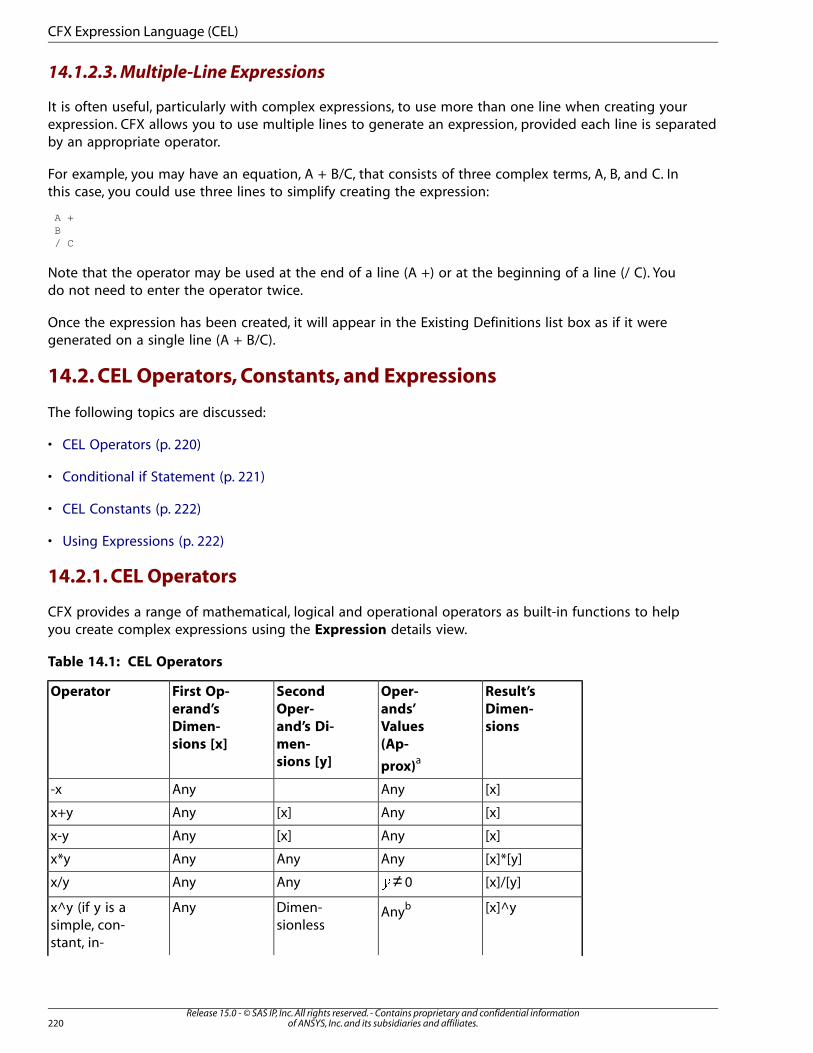
14.1.2.3. Multiple-Line Expressions
It is often useful, particularly with complex expressions, to use more than one line when creating yourexpression. CFX allows you to use multiple lines to generate an expression, provided each line is separatedby an appropriate operator.
For example, you may have an equation, A + B/C, that consists of three complex terms, A, B, and C. Inthis case, you could use three lines to simplify creating the expression:
A +B/ C
Note that the operator may be used at the end of a line (A +) or at the beginning of a line (/ C). Youdo not need to enter the operator twice.
Once the expression has been created, it will appear in the Existing Definitions list box as if it weregenerated on a single line (A + B/C).
14.2. CEL Operators, Constants, and Expressions
The following topics are discussed:
• CEL Operators (p. 220)
• Conditional if Statement (p. 221)
• CEL Constants (p. 222)
• Using Expressions (p. 222)
14.2.1. CEL Operators
CFX provides a range of mathematical, logical and operational operators as built-in functions to helpyou create complex expressions using the Expression details view.
Table 14.1: CEL Operators
Result’s
Dimen-
sions
Oper-
ands’
Values
(Ap-
prox)a
Second
Oper-
and’s Di-
men-
sions [y]
First Op-
erand’s
Dimen-
sions [x]
Operator
[x]AnyAny-x
[x]Any[x]Anyx+y
[x]Any[x]Anyx-y
[x]*[y]AnyAnyAnyx*y
[x]/[y]≠� 0AnyAnyx/y
[x]^yAnybDimen-sionless
Anyx^y (if y is asimple, con-stant, in-
Release 15.0 - © SAS IP, Inc. All rights reserved. - Contains proprietary and confidential informationof ANSYS, Inc. and its subsidiaries and affiliates.220
CFX Expression Language (CEL)
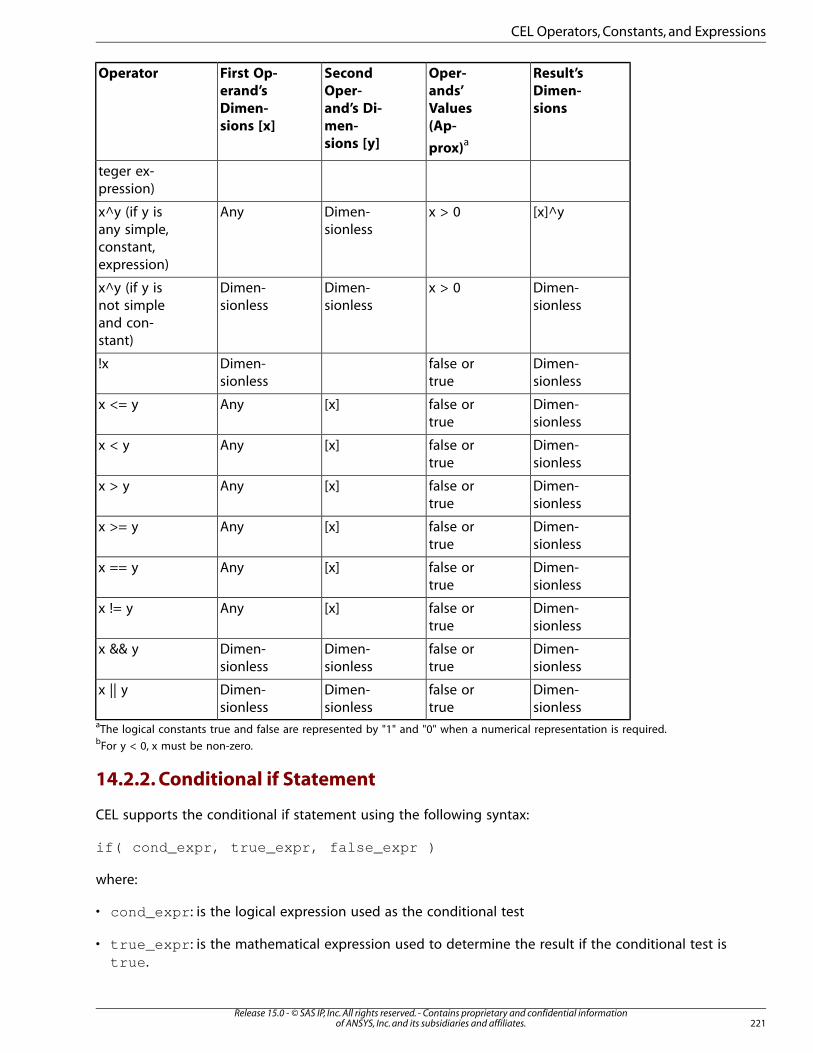
Result’s
Dimen-
sions
Oper-
ands’
Values
(Ap-
prox)a
Second
Oper-
and’s Di-
men-
sions [y]
First Op-
erand’s
Dimen-
sions [x]
Operator
teger ex-pression)
[x]^yx > 0Dimen-sionless
Anyx^y (if y isany simple,constant,expression)
Dimen-sionless
x > 0Dimen-sionless
Dimen-sionless
x^y (if y isnot simpleand con-stant)
Dimen-sionless
false ortrue
Dimen-sionless
!x
Dimen-sionless
false ortrue
[x]Anyx <= y
Dimen-sionless
false ortrue
[x]Anyx < y
Dimen-sionless
false ortrue
[x]Anyx > y
Dimen-sionless
false ortrue
[x]Anyx >= y
Dimen-sionless
false ortrue
[x]Anyx == y
Dimen-sionless
false ortrue
[x]Anyx != y
Dimen-sionless
false ortrue
Dimen-sionless
Dimen-sionless
x && y
Dimen-sionless
false ortrue
Dimen-sionless
Dimen-sionless
x || y
aThe logical constants true and false are represented by "1" and "0" when a numerical representation is required.bFor y < 0, x must be non-zero.
14.2.2. Conditional if Statement
CEL supports the conditional if statement using the following syntax:
if( cond_expr, true_expr, false_expr )
where:
• cond_expr : is the logical expression used as the conditional test
• true_expr : is the mathematical expression used to determine the result if the conditional test istrue .
221Release 15.0 - © SAS IP, Inc. All rights reserved. - Contains proprietary and confidential information
of ANSYS, Inc. and its subsidiaries and affiliates.
CEL Operators, Constants, and Expressions
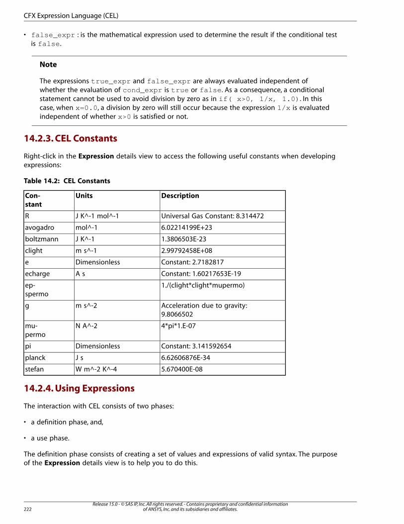
• false_expr : is the mathematical expression used to determine the result if the conditional testis false .
Note
The expressions true_expr and false_expr are always evaluated independent ofwhether the evaluation of cond_expr is true or false . As a consequence, a conditionalstatement cannot be used to avoid division by zero as in if( x>0, 1/x, 1.0) . In thiscase, when x=0.0 , a division by zero will still occur because the expression 1/x is evaluatedindependent of whether x>0 is satisfied or not.
14.2.3. CEL Constants
Right-click in the Expression details view to access the following useful constants when developingexpressions:
Table 14.2: CEL Constants
DescriptionUnitsCon-
stant
Universal Gas Constant: 8.314472J K^-1 mol^-1R
6.02214199E+23mol^-1avogadro
1.3806503E-23J K^-1boltzmann
2.99792458E+08m s^-1clight
Constant: 2.7182817Dimensionlesse
Constant: 1.60217653E-19A secharge
1./(clight*clight*mupermo)ep-spermo
Acceleration due to gravity:9.8066502
m s^-2g
4*pi*1.E-07N A^-2mu-permo
Constant: 3.141592654Dimensionlesspi
6.62606876E-34J splanck
5.670400E-08W m^-2 K^-4stefan
14.2.4. Using Expressions
The interaction with CEL consists of two phases:
• a definition phase, and,
• a use phase.
The definition phase consists of creating a set of values and expressions of valid syntax. The purposeof the Expression details view is to help you to do this.
Release 15.0 - © SAS IP, Inc. All rights reserved. - Contains proprietary and confidential informationof ANSYS, Inc. and its subsidiaries and affiliates.222
CFX Expression Language (CEL)

14.2.4.1. Use of Offset Temperature
When using temperature values in expressions, it is generally safer to use units of [K] only. When unitsare used that posses an offset (for example, [C]), they are converted internally to [K]. For terms thathave temperature to the power of unity, any unit conversion will include the offset between temperaturescales. However, in all other cases the offset is ignored because this is usually the most appropriatebehavior. You should therefore take care when specifying an expression involving non-unit powers oftemperature. For example, each of the expressions below is equivalent:
Temperature = 30 [C]Temperature = 303.15 [K]Temperature = 0 [C] + 30 [K]Temperature = 273.15 [K] + 30 [K]
These are only equivalent because all units are to the power of unity and units other than [K] appearno more than once in each expression. The following expression will not produce the expected result:
Temperature = 0 [C] + 30 [C]
This is equivalent to 576.30 [K] because each value is converted to [K] and then summed. The twoexpression below are equivalent (as expected) because the offset in scales is ignored for non-unit powersof temperature:
Specific Heat = 4200 [J kg^-1 C^-1]Specific Heat = 4200 [J kg^-1 K^-1]
14.3. CEL Examples
The following examples are included in this section:
• Example: Reynolds Number Dependent Viscosity (p. 223)
• Example: Feedback to Control Inlet Temperature (p. 224)
14.3.1. Example: Reynolds Number Dependent Viscosity
In this example it is assumed that some of the fluid properties, including the dynamic viscosity, are notknown. However the Reynolds number, inlet velocity and a length scale are known. The flow is com-pressible and therefore the density is variable.
Given this information it is possible to calculate the fluid dynamic viscosity based on the Reynoldsnumber. The Reynolds number is given by:
=��� � �
�
where � is density, U a velocity scale, L a length scale and � the dynamic viscosity. The velocity scaleis taken as the inlet velocity, the length scale as the inlet width and the density is calculated as the av-erage density over the inlet area.
The LIBRARY section of the CCL (CFX Command Language) file appears as follows:
LIBRARY : CEL : EXPRESSIONS : Re = 4.29E6 [ ] Vel = 60 [m s^-1] L=1.044[m]
223Release 15.0 - © SAS IP, Inc. All rights reserved. - Contains proprietary and confidential information
of ANSYS, Inc. and its subsidiaries and affiliates.
CEL Examples
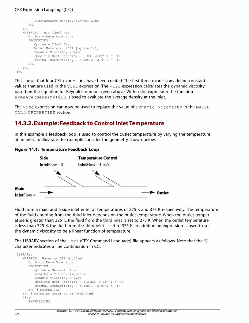
Visc=areaAve(density)@in*Vel*L/Re END END MATERIAL : Air Ideal Gas Option = Pure Substance PROPERTIES : Option = Ideal Gas Molar Mass = 2.896E1 [kg kmol^-1] Dynamic Viscosity = Visc Specific Heat Capacity = 1.E3 [J kg^-1 K^-1] Thermal Conductivity = 2.52E-2 [W m^-1 K^-1] END ENDEND
This shows that four CEL expressions have been created. The first three expressions define constantvalues that are used in the Visc expression. The Visc expression calculates the dynamic viscositybased on the equation for Reynolds number given above. Within the expression the functionareaAve(density)@in is used to evaluate the average density at the inlet.
The Visc expression can now be used to replace the value of Dynamic Viscosity in the MATERIAL > PROPERTIES section.
14.3.2. Example: Feedback to Control Inlet Temperature
In this example a feedback loop is used to control the outlet temperature by varying the temperatureat an inlet. To illustrate the example consider the geometry shown below:
Figure 14.1: Temperature Feedback Loop
Fluid from a main and a side inlet enter at temperatures of 275 K and 375 K respectively. The temperatureof the fluid entering from the third inlet depends on the outlet temperature. When the outlet temper-ature is greater than 325 K, the fluid from the third inlet is set to 275 K. When the outlet temperatureis less than 325 K, the fluid from the third inlet is set to 375 K. In addition an expression is used to setthe dynamic viscosity to be a linear function of temperature.
The LIBRARY section of the .ccl (CFX Command Language) file appears as follows. Note that the “\”character indicates a line continuation in CCL.
LIBRARY: MATERIAL: Water at STP Modified Option = Pure Substance PROPERTIES: Option = General Fluid Density = 9.999E2 [kg m^-3] Dynamic Viscosity = VisT Specific Heat Capacity = 4.21E3 [J kg^-1 K^-1] Thermal Conductivity = 5.69E-1 [W m^-1 K^-1] END # PROPERTIES END # MATERIAL Water at STP Modified CEL: EXPRESSIONS:
Release 15.0 - © SAS IP, Inc. All rights reserved. - Contains proprietary and confidential informationof ANSYS, Inc. and its subsidiaries and affiliates.224
CFX Expression Language (CEL)
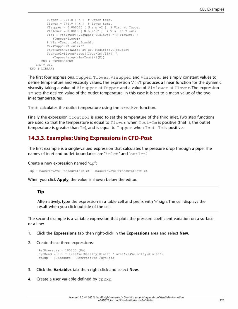
Tupper = 375.0 [ K ] # Upper temp. Tlower = 275.0 [ K ] # Lower temp. Visupper = 0.000545 [ N s m^-2 ] # Vis. at Tupper Vislower = 0.0018 [ N s m^-2 ] # Vis. at Tlower VisT = Vislower+(Visupper-Vislower)*(T-Tlower)/ \ (Tupper-Tlower) # Vis.-Temp. relationship Tm=(Tupper+Tlower)/2 Tout=areaAve(Water at STP Modified.T)@outlet Tcontrol=Tlower*step((Tout-Tm)/1[K]) \ +Tupper*step((Tm-Tout)/1[K]) END # EXPRESSIONS END # CELEND # LIBRARY
The first four expressions, Tupper , Tlower , Visupper and Vislower are simply constant values todefine temperature and viscosity values. The expression VisT produces a linear function for the dynamicviscosity taking a value of Visupper at Tupper and a value of Vislower at Tlower . The expressionTm sets the desired value of the outlet temperature. In this case it is set to a mean value of the twoinlet temperatures.
Tout calculates the outlet temperature using the areaAve function.
Finally the expression Tcontrol is used to set the temperature of the third inlet. Two step functionsare used so that the temperature is equal to Tlower when Tout-Tm is positive (that is, the outlettemperature is greater than Tm), and is equal to Tupper when Tout-Tm is positive.
14.3.3. Examples: Using Expressions in CFD-Post
The first example is a single-valued expression that calculates the pressure drop through a pipe. Thenames of inlet and outlet boundaries are “inlet ” and “outlet ”.
Create a new expression named “dp”:
dp = massFlowAve(Pressure)@inlet – massFlowAve(Pressure)@outlet
When you click Apply, the value is shown below the editor.
Tip
Alternatively, type the expression in a table cell and prefix with ‘=’ sign. The cell displays theresult when you click outside of the cell.
The second example is a variable expression that plots the pressure coefficient variation on a surfaceor a line:
1. Click the Expressions tab, then right-click in the Expressions area and select New.
2. Create these three expressions:
RefPressure = 100000 [Pa]dynHead = 0.5 * areaAve(Density)@inlet * areaAve(Velocity)@inlet^2cpExp = (Pressure - RefPressure)/dynHead
3. Click the Variables tab, then right-click and select New.
4. Create a user variable defined by cpExp .
225Release 15.0 - © SAS IP, Inc. All rights reserved. - Contains proprietary and confidential information
of ANSYS, Inc. and its subsidiaries and affiliates.
CEL Examples

5. Select Insert > Location > Line and use the details view to position the line in the simulation.
From the details view Color tab, plot the user variable on a surface or a line (just as you wouldwith any other variable).
14.4. CEL Technical Details
CEL is a byte code compiled language. Compiled languages, such as Fortran, rely on a translation programto convert them into the native machine language of the host platform. Interpreted languages are oftwo types: the fully interpreted languages such as the UNIX C shell, and the byte code compiled languagessuch as CEL. With byte codes, host machines are loaded with a client program (written in a compiledlanguage and compiled for that machine architecture) that interprets the byte stream. The advantageof the byte code is that they can be the same on all host platforms, obviating the need for platformdependent codes.
Because the byte codes are interpreted, there is no need to re-link executable programs to perform adifferent calculation. Furthermore, many of the problems encountered by writing and linking in separateroutines, for instance in C or Fortran, are averted, and the time taken to set up and debug complicatedproblems reduced considerably.
The link between CEL and the CFX-Solver is accomplished through an internal program called genicode.Genicode generates intermediate code from your CEL definitions and writes to a file that is then inter-preted by the CFX-Solver during the solution process.
Release 15.0 - © SAS IP, Inc. All rights reserved. - Contains proprietary and confidential informationof ANSYS, Inc. and its subsidiaries and affiliates.226
CFX Expression Language (CEL)

Chapter 15: Functions in ANSYS CFX
This chapter describes predefined functions in ANSYS CFX:15.1. CEL Mathematical Functions15.2. Quantitative CEL Functions in ANSYS CFX15.3. Functions Involving Coordinates15.4. CEL Functions with Multiphase Flow15.5. Quantitative Function List
15.1. CEL Mathematical Functions
The following mathematical functions are available for use with all CEL expressions.
Note
In the Function column in the table below, [a] denotes any dimension of the first operand.
Table 15.1: Standard Mathematical CEL Functions
Result’s DimensionsOperand’s ValuesFunction
[a]Anyabs( [a] )
Radians− ≤ ≤�acos( [ ] )
Radians− ≤ ≤�asin( [ ] )
RadiansAnyatan( [ ] )a
RadiansAnyatan2( [a], [a] )a
Dimensionless≤ �besselJ( [ ], [ ] )b
Dimensionless≤ �besselY( [ ], [ ] )b
DimensionlessAnycos( [radians] )
DimensionlessAnycosh( [ ] )
DimensionlessAnyexp( [ ] )
DimensionlessDimensionlessint([ ])c
Dimensionless< �loge( [ ] )d
Dimensionless< �log10( [ ] )e
[a]Anymin( [a], [a] )
[a]Anymax( [a], [a] )
[a]Anymod( [a], [a] )f
DimensionlessDimensionlessnint([ ])g
DimensionlessAnysin( [radians] )
227Release 15.0 - © SAS IP, Inc. All rights reserved. - Contains proprietary and confidential information
of ANSYS, Inc. and its subsidiaries and affiliates.
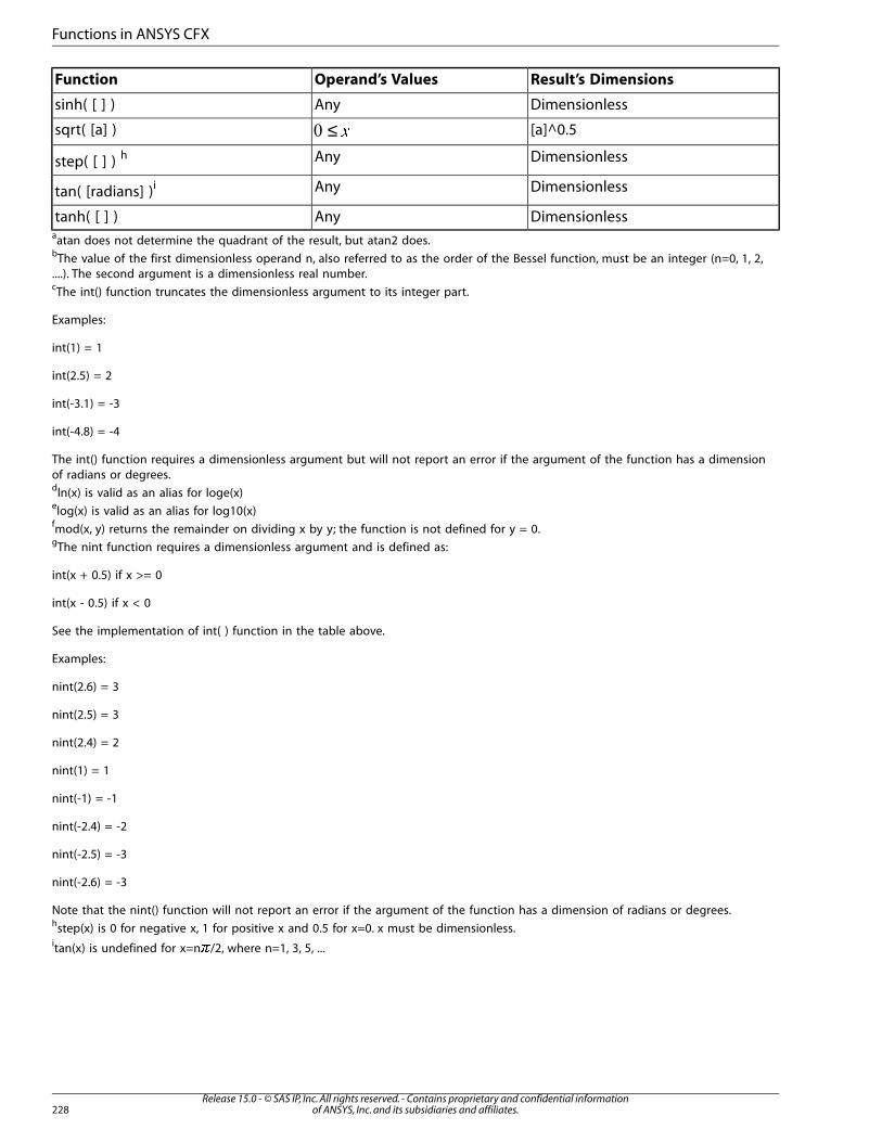
Result’s DimensionsOperand’s ValuesFunction
DimensionlessAnysinh( [ ] )
[a]^0.5≤ �sqrt( [a] )
DimensionlessAnystep( [ ] ) h
DimensionlessAnytan( [radians] )i
DimensionlessAnytanh( [ ] )aatan does not determine the quadrant of the result, but atan2 does.bThe value of the first dimensionless operand n, also referred to as the order of the Bessel function, must be an integer (n=0, 1, 2,....). The second argument is a dimensionless real number.cThe int() function truncates the dimensionless argument to its integer part.
Examples:
int(1) = 1
int(2.5) = 2
int(-3.1) = -3
int(-4.8) = -4
The int() function requires a dimensionless argument but will not report an error if the argument of the function has a dimensionof radians or degrees.dln(x) is valid as an alias for loge(x)elog(x) is valid as an alias for log10(x)fmod(x, y) returns the remainder on dividing x by y; the function is not defined for y = 0.gThe nint function requires a dimensionless argument and is defined as:
int(x + 0.5) if x >= 0
int(x - 0.5) if x < 0
See the implementation of int( ) function in the table above.
Examples:
nint(2.6) = 3
nint(2.5) = 3
nint(2.4) = 2
nint(1) = 1
nint(-1) = -1
nint(-2.4) = -2
nint(-2.5) = -3
nint(-2.6) = -3
Note that the nint() function will not report an error if the argument of the function has a dimension of radians or degrees.hstep(x) is 0 for negative x, 1 for positive x and 0.5 for x=0. x must be dimensionless.itan(x) is undefined for x=n�/2, where n=1, 3, 5, ...
Release 15.0 - © SAS IP, Inc. All rights reserved. - Contains proprietary and confidential informationof ANSYS, Inc. and its subsidiaries and affiliates.228
Functions in ANSYS CFX
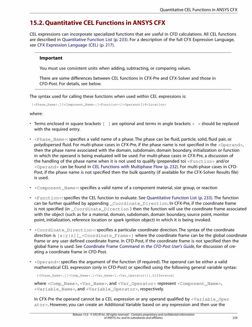
15.2. Quantitative CEL Functions in ANSYS CFX
CEL expressions can incorporate specialized functions that are useful in CFD calculations. All CEL functionsare described in Quantitative Function List (p. 233). For a description of the full CFX Expression Language,see CFX Expression Language (CEL) (p. 217).
Important
You must use consistent units when adding, subtracting, or comparing values.
There are some differences between CEL functions in CFX-Pre and CFX-Solver and those inCFD-Post. For details, see below.
The syntax used for calling these functions when used within CEL expressions is:
[<Phase_Name>.][<Component_Name>.]<Function>([<Operand>])@<Location>
where:
• Terms enclosed in square brackets [ ] are optional and terms in angle brackets < > should be replacedwith the required entry.
• <Phase_Name>: specifies a valid name of a phase. The phase can be fluid, particle, solid, fluid pair, orpolydispersed fluid. For multi-phase cases in CFX-Pre, if the phase name is not specified in the <Operand> ,then the phase name associated with the domain, subdomain, domain boundary, initialization or functionin which the operand is being evaluated will be used. For multi-phase cases in CFX-Pre, a discussion ofthe handling of the phase name when it is not used to qualify (prepended to) <Function> and/or<Operand> can be found in CEL Functions with Multiphase Flow (p. 232). For multi-phase cases in CFD-Post, if the phase name is not specified then the bulk quantity (if available for the CFX-Solver Results file)is used.
• <Component_Name>: specifies a valid name of a component material, size group, or reaction
• <Function> : specifies the CEL function to evaluate. See Quantitative Function List (p. 233). The functioncan be further qualified by appending _Coordinate_Direction . In CFX-Pre, if the coordinate frameis not specified (in _Coordinate_Direction ) then the function will use the coordinate frame associatedwith the object (such as for a material, domain, subdomain, domain boundary, source point, monitorpoint, initialization, reference location or spark ignition object) in which it is being invoked.
• <Coordinate_Direction> : specifies a particular coordinate direction. The syntax of the coordinatedirection is [x|y|z][_<Coordinate_Frame>] where the coordinate frame can be the global coordinateframe or any user defined coordinate frame. In CFD-Post, if the coordinate frame is not specified then theglobal frame is used. See Coordinate Frame Command in the CFD-Post User's Guide, for discussion of cre-ating a coordinate frame in CFD-Post.
• <Operand> : specifies the argument of the function (if required). The operand can be either a validmathematical CEL expression (only in CFD-Post) or specified using the following general variable syntax:
[<Phase_Name>.][<Comp_Name>.]<Var_Name>[.<Var_Operator>][.Difference]
where <Comp_Name>, <Var_Name>, and <Var_Operator> represent <Component_Name>,<Variable_Name> , and <Variable_Operator> , respectively.
In CFX-Pre the operand cannot be a CEL expression or any operand qualified by <Variable_Operator> . However, you can create an Additional Variable based on any expression and then use the
229Release 15.0 - © SAS IP, Inc. All rights reserved. - Contains proprietary and confidential information
of ANSYS, Inc. and its subsidiaries and affiliates.
Quantitative CEL Functions in ANSYS CFX
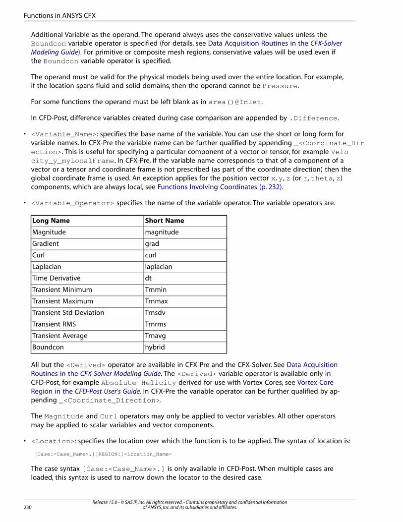
Additional Variable as the operand. The operand always uses the conservative values unless theBoundcon variable operator is specified (for details, see Data Acquisition Routines in the CFX-Solver
Modeling Guide). For primitive or composite mesh regions, conservative values will be used even ifthe Boundcon variable operator is specified.
The operand must be valid for the physical models being used over the entire location. For example,if the location spans fluid and solid domains, then the operand cannot be Pressure .
For some functions the operand must be left blank as in area()@Inlet .
In CFD-Post, difference variables created during case comparison are appended by .Difference .
• <Variable_Name> : specifies the base name of the variable. You can use the short or long form forvariable names. In CFX-Pre the variable name can be further qualified by appending _<Coordinate_Direction> . This is useful for specifying a particular component of a vector or tensor, for example Velocity_y_myLocalFrame . In CFX-Pre, if the variable name corresponds to that of a component of avector or a tensor and coordinate frame is not prescribed (as part of the coordinate direction) then theglobal coordinate frame is used. An exception applies for the position vector x , y , z (or r , theta , z )components, which are always local, see Functions Involving Coordinates (p. 232).
• <Variable_Operator> specifies the name of the variable operator. The variable operators are.
Short NameLong Name
magnitudeMagnitude
gradGradient
curlCurl
laplacianLaplacian
dtTime Derivative
TrnminTransient Minimum
TrnmaxTransient Maximum
TrnsdvTransient Std Deviation
TrnrmsTransient RMS
TrnavgTransient Average
hybridBoundcon
All but the <Derived> operator are available in CFX-Pre and the CFX-Solver. See Data AcquisitionRoutines in the CFX-Solver Modeling Guide. The <Derived> variable operator is available only inCFD-Post, for example Absolute Helicity derived for use with Vortex Cores, see Vortex CoreRegion in the CFD-Post User's Guide. In CFX-Pre the variable operator can be further qualified by ap-pending _<Coordinate_Direction> .
The Magnitude and Curl operators may only be applied to vector variables. All other operatorsmay be applied to scalar variables and vector components.
• <Location> : specifies the location over which the function is to be applied. The syntax of location is:
[Case:<Case_Name>.][REGION:]<Location_Name>
The case syntax [Case:<Case_Name>.] is only available in CFD-Post. When multiple cases areloaded, this syntax is used to narrow down the locator to the desired case.
Release 15.0 - © SAS IP, Inc. All rights reserved. - Contains proprietary and confidential informationof ANSYS, Inc. and its subsidiaries and affiliates.230
Functions in ANSYS CFX
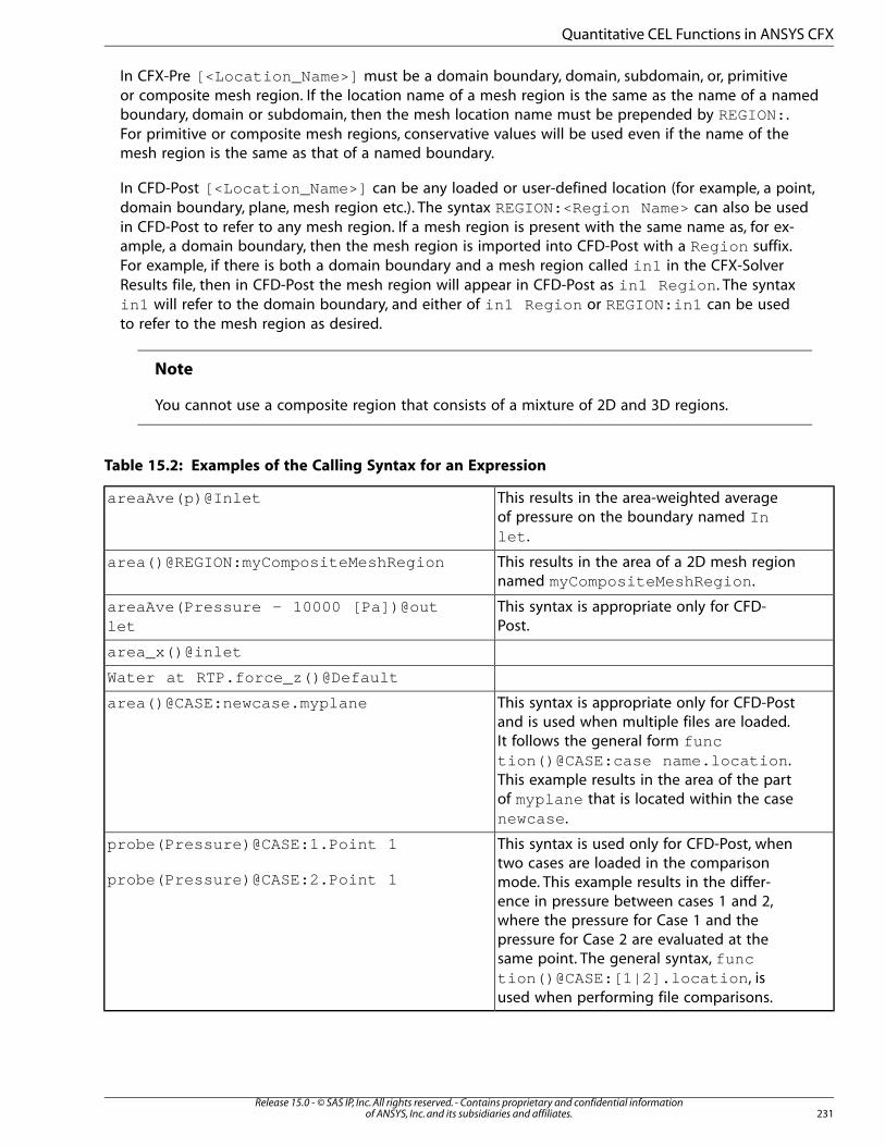
In CFX-Pre [<Location_Name>] must be a domain boundary, domain, subdomain, or, primitiveor composite mesh region. If the location name of a mesh region is the same as the name of a namedboundary, domain or subdomain, then the mesh location name must be prepended by REGION:.For primitive or composite mesh regions, conservative values will be used even if the name of themesh region is the same as that of a named boundary.
In CFD-Post [<Location_Name>] can be any loaded or user-defined location (for example, a point,domain boundary, plane, mesh region etc.). The syntax REGION:<Region Name> can also be usedin CFD-Post to refer to any mesh region. If a mesh region is present with the same name as, for ex-ample, a domain boundary, then the mesh region is imported into CFD-Post with a Region suffix.For example, if there is both a domain boundary and a mesh region called in1 in the CFX-SolverResults file, then in CFD-Post the mesh region will appear in CFD-Post as in1 Region . The syntaxin1 will refer to the domain boundary, and either of in1 Region or REGION:in1 can be usedto refer to the mesh region as desired.
Note
You cannot use a composite region that consists of a mixture of 2D and 3D regions.
Table 15.2: Examples of the Calling Syntax for an Expression
This results in the area-weighted averageof pressure on the boundary named Inlet .
areaAve(p)@Inlet
This results in the area of a 2D mesh regionnamed myCompositeMeshRegion .
area()@REGION:myCompositeMeshRegion
This syntax is appropriate only for CFD-Post.
areaAve(Pressure - 10000 [Pa])@outlet
area_x()@inlet
Water at RTP.force_z()@Default
This syntax is appropriate only for CFD-Postand is used when multiple files are loaded.
area()@CASE:newcase.myplane
It follows the general form function()@CASE:case name.location .This example results in the area of the partof myplane that is located within the casenewcase .
This syntax is used only for CFD-Post, whentwo cases are loaded in the comparison
probe(Pressure)@CASE:1.Point 1
probe(Pressure)@CASE:2.Point 1 mode. This example results in the differ-ence in pressure between cases 1 and 2,where the pressure for Case 1 and thepressure for Case 2 are evaluated at thesame point. The general syntax, function()@CASE:[1|2].location , isused when performing file comparisons.
231Release 15.0 - © SAS IP, Inc. All rights reserved. - Contains proprietary and confidential information
of ANSYS, Inc. and its subsidiaries and affiliates.
Quantitative CEL Functions in ANSYS CFX

15.3. Functions Involving Coordinates
The CEL variables x , y , z , r and theta , representing the local coordinates, cannot be used as thevariable. However, the variables xGlobal , yGlobal and zGlobal can be used. For example, thefollowing is a valid expression definition:
z*areaAve(xGlobal)@inlet
15.4. CEL Functions with Multiphase Flow
Note
These functions are available in CFX-Pre and CFX-Solver without restrictions, and in CFD-Postwith the restriction that you cannot use short names.
If the function is fluid-specific, various behaviors are possible depending on the function type:
• For massFlow and massFlowAve , if the phase name is not specified for the function, then the bulkmass flows will be used. See cases 1 to 7 in the table below.
• For other fluid-specific functions:
– if a fluid-specific operand is specified and no fluid is specified for the function, then the fluid specifiedfor the operand will be assumed for the function as well. See case 8 in the table below.
– if the function is specified and no fluid is specified for the operand, then the fluid specified for thefunction will be assumed for the operand as well. See cases 7 and 9 in the table below.
• If both the function or operand are fluid-specific, and a phase name is not given for either, the solver willstop with an error. See case 10 in the table below.
Table 15.3: CEL Multiphase Examples
BehaviorCEL Function - MultiphaseCase
Bulk mass flow rate through inletmassFlow()@inlet1
Air mass flow rate through inletAir.massFlow()@inlet2
Bulk mass flow averaged pressure on inletmassFlowAve(Pressure)@inlet3
Air mass flow averaged pressure on inletAir.massFlowAve(Pressure)@inlet
4
Bulk mass flow averaged air volume fractionon inlet
massFlowAve(Air.Volume Fraction)@inlet
5
Air mass flow averaged air volume fractionon inlet
Air.massFlowAve(Air.VolumeFraction)@inlet
6
Same as Air.massFlowAve(Air.VolumeFraction)@ inlet
Air.massFlowAve(Volume Fraction)@inlet
7
Same as Air.massInt(Air.VolumeFraction)@ domain1
massInt(Air.Volume Fraction)@domain1
8
Same as Air.massInt(Air.VolumeFraction)@ domain1
Air.massInt(Volume Fraction)@domain1
9
Release 15.0 - © SAS IP, Inc. All rights reserved. - Contains proprietary and confidential informationof ANSYS, Inc. and its subsidiaries and affiliates.232
Functions in ANSYS CFX
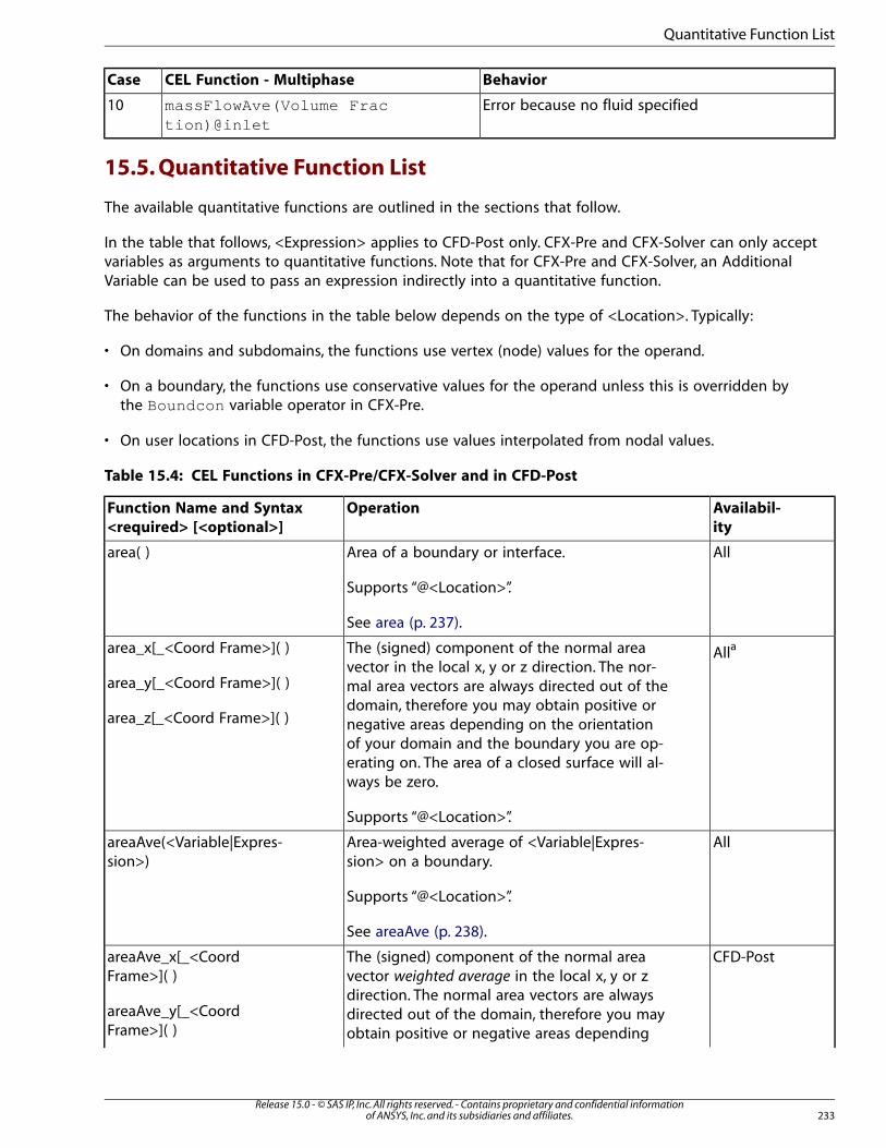
BehaviorCEL Function - MultiphaseCase
Error because no fluid specifiedmassFlowAve(Volume Fraction)@inlet
10
15.5. Quantitative Function List
The available quantitative functions are outlined in the sections that follow.
In the table that follows, <Expression> applies to CFD-Post only. CFX-Pre and CFX-Solver can only acceptvariables as arguments to quantitative functions. Note that for CFX-Pre and CFX-Solver, an AdditionalVariable can be used to pass an expression indirectly into a quantitative function.
The behavior of the functions in the table below depends on the type of <Location>. Typically:
• On domains and subdomains, the functions use vertex (node) values for the operand.
• On a boundary, the functions use conservative values for the operand unless this is overridden bythe Boundcon variable operator in CFX-Pre.
• On user locations in CFD-Post, the functions use values interpolated from nodal values.
Table 15.4: CEL Functions in CFX-Pre/CFX-Solver and in CFD-Post
Availabil-
ity
OperationFunction Name and Syntax
<required> [<optional>]
AllArea of a boundary or interface.area( )
Supports “@<Location>”.
See area (p. 237).
AllaThe (signed) component of the normal areavector in the local x, y or z direction. The nor-
area_x[_<Coord Frame>]( )
area_y[_<Coord Frame>]( ) mal area vectors are always directed out of the
area_z[_<Coord Frame>]( )domain, therefore you may obtain positive ornegative areas depending on the orientationof your domain and the boundary you are op-erating on. The area of a closed surface will al-ways be zero.
Supports “@<Location>”.
AllArea-weighted average of <Variable|Expres-sion> on a boundary.
areaAve(<Variable|Expres-sion>)
Supports “@<Location>”.
See areaAve (p. 238).
CFD-PostThe (signed) component of the normal areavector weighted average in the local x, y or z
areaAve_x[_<CoordFrame>]( )
direction. The normal area vectors are alwaysareaAve_y[_<CoordFrame>]( )
directed out of the domain, therefore you mayobtain positive or negative areas depending
233Release 15.0 - © SAS IP, Inc. All rights reserved. - Contains proprietary and confidential information
of ANSYS, Inc. and its subsidiaries and affiliates.
Quantitative Function List
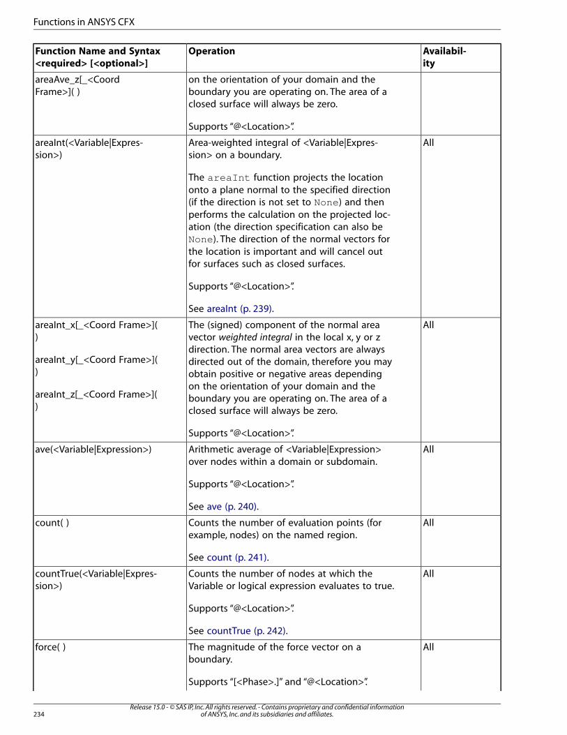
Availabil-
ity
OperationFunction Name and Syntax
<required> [<optional>]
areaAve_z[_<CoordFrame>]( )
on the orientation of your domain and theboundary you are operating on. The area of aclosed surface will always be zero.
Supports “@<Location>”.
AllArea-weighted integral of <Variable|Expres-sion> on a boundary.
areaInt(<Variable|Expres-sion>)
The areaInt function projects the locationonto a plane normal to the specified direction(if the direction is not set to None) and thenperforms the calculation on the projected loc-ation (the direction specification can also beNone). The direction of the normal vectors forthe location is important and will cancel outfor surfaces such as closed surfaces.
Supports “@<Location>”.
See areaInt (p. 239).
AllThe (signed) component of the normal areavector weighted integral in the local x, y or z
areaInt_x[_<Coord Frame>]()
direction. The normal area vectors are alwaysareaInt_y[_<Coord Frame>]()
directed out of the domain, therefore you mayobtain positive or negative areas depending
areaInt_z[_<Coord Frame>]()
on the orientation of your domain and theboundary you are operating on. The area of aclosed surface will always be zero.
Supports “@<Location>”.
AllArithmetic average of <Variable|Expression>over nodes within a domain or subdomain.
ave(<Variable|Expression>)
Supports “@<Location>”.
See ave (p. 240).
AllCounts the number of evaluation points (forexample, nodes) on the named region.
count( )
See count (p. 241).
AllCounts the number of nodes at which theVariable or logical expression evaluates to true.
countTrue(<Variable|Expres-sion>)
Supports “@<Location>”.
See countTrue (p. 242).
AllThe magnitude of the force vector on aboundary.
force( )
Supports “[<Phase>.]” and “@<Location>”.
Release 15.0 - © SAS IP, Inc. All rights reserved. - Contains proprietary and confidential informationof ANSYS, Inc. and its subsidiaries and affiliates.234
Functions in ANSYS CFX
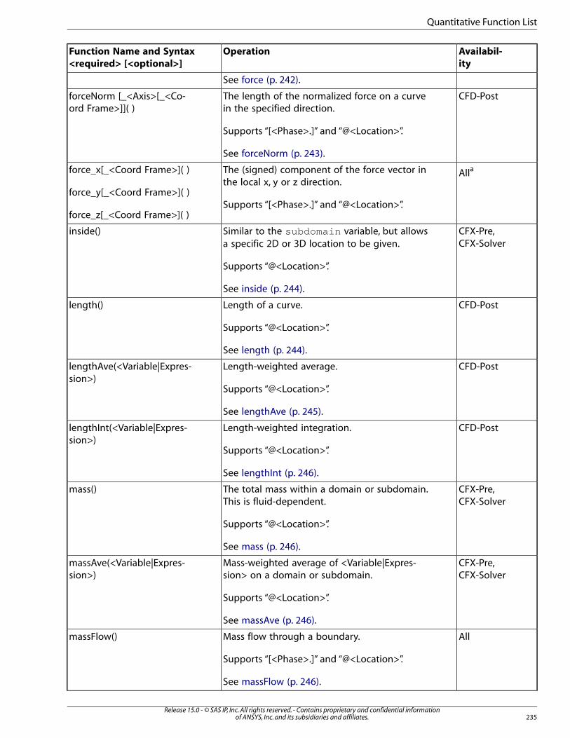
Availabil-
ity
OperationFunction Name and Syntax
<required> [<optional>]
See force (p. 242).
CFD-PostThe length of the normalized force on a curvein the specified direction.
forceNorm [_<Axis>[_<Co-ord Frame>]]( )
Supports “[<Phase>.]” and “@<Location>”.
See forceNorm (p. 243).
AllaThe (signed) component of the force vector inthe local x, y or z direction.
force_x[_<Coord Frame>]( )
force_y[_<Coord Frame>]( )Supports “[<Phase>.]” and “@<Location>”.
force_z[_<Coord Frame>]( )
CFX-Pre,CFX-Solver
Similar to the subdomain variable, but allowsa specific 2D or 3D location to be given.
inside()
Supports “@<Location>”.
See inside (p. 244).
CFD-PostLength of a curve.length()
Supports “@<Location>”.
See length (p. 244).
CFD-PostLength-weighted average.lengthAve(<Variable|Expres-sion>)
Supports “@<Location>”.
See lengthAve (p. 245).
CFD-PostLength-weighted integration.lengthInt(<Variable|Expres-sion>)
Supports “@<Location>”.
See lengthInt (p. 246).
CFX-Pre,CFX-Solver
The total mass within a domain or subdomain.This is fluid-dependent.
mass()
Supports “@<Location>”.
See mass (p. 246).
CFX-Pre,CFX-Solver
Mass-weighted average of <Variable|Expres-sion> on a domain or subdomain.
massAve(<Variable|Expres-sion>)
Supports “@<Location>”.
See massAve (p. 246).
AllMass flow through a boundary.massFlow()
Supports “[<Phase>.]” and “@<Location>”.
See massFlow (p. 246).
235Release 15.0 - © SAS IP, Inc. All rights reserved. - Contains proprietary and confidential information
of ANSYS, Inc. and its subsidiaries and affiliates.
Quantitative Function List
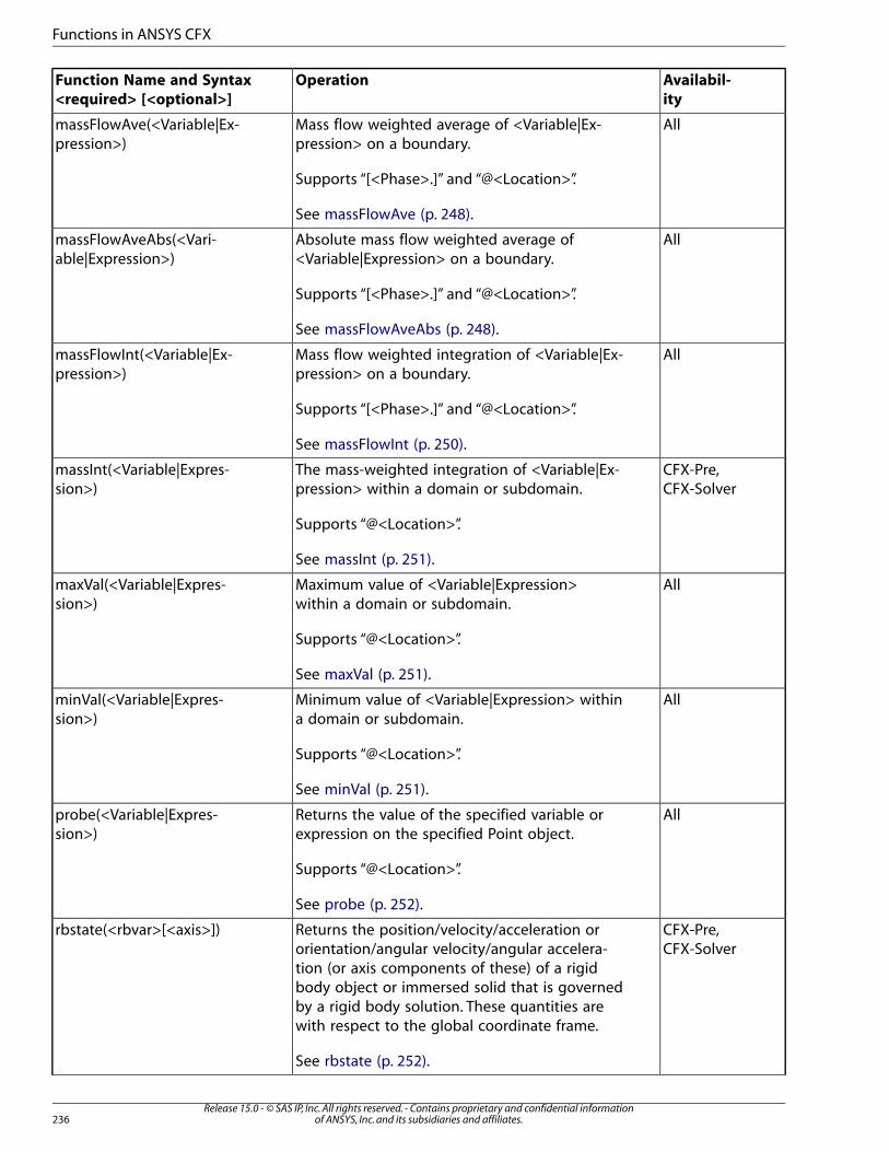
Availabil-
ity
OperationFunction Name and Syntax
<required> [<optional>]
AllMass flow weighted average of <Variable|Ex-pression> on a boundary.
massFlowAve(<Variable|Ex-pression>)
Supports “[<Phase>.]” and “@<Location>”.
See massFlowAve (p. 248).
AllAbsolute mass flow weighted average of<Variable|Expression> on a boundary.
massFlowAveAbs(<Vari-able|Expression>)
Supports “[<Phase>.]” and “@<Location>”.
See massFlowAveAbs (p. 248).
AllMass flow weighted integration of <Variable|Ex-pression> on a boundary.
massFlowInt(<Variable|Ex-pression>)
Supports “[<Phase>.]” and “@<Location>”.
See massFlowInt (p. 250).
CFX-Pre,CFX-Solver
The mass-weighted integration of <Variable|Ex-pression> within a domain or subdomain.
massInt(<Variable|Expres-sion>)
Supports “@<Location>”.
See massInt (p. 251).
AllMaximum value of <Variable|Expression>within a domain or subdomain.
maxVal(<Variable|Expres-sion>)
Supports “@<Location>”.
See maxVal (p. 251).
AllMinimum value of <Variable|Expression> withina domain or subdomain.
minVal(<Variable|Expres-sion>)
Supports “@<Location>”.
See minVal (p. 251).
AllReturns the value of the specified variable orexpression on the specified Point object.
probe(<Variable|Expres-sion>)
Supports “@<Location>”.
See probe (p. 252).
CFX-Pre,CFX-Solver
Returns the position/velocity/acceleration ororientation/angular velocity/angular accelera-
rbstate(<rbvar>[<axis>])
tion (or axis components of these) of a rigidbody object or immersed solid that is governedby a rigid body solution. These quantities arewith respect to the global coordinate frame.
See rbstate (p. 252).
Release 15.0 - © SAS IP, Inc. All rights reserved. - Contains proprietary and confidential informationof ANSYS, Inc. and its subsidiaries and affiliates.236
Functions in ANSYS CFX
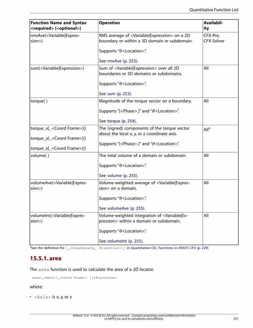
Availabil-
ity
OperationFunction Name and Syntax
<required> [<optional>]
CFX-Pre,CFX-Solver
RMS average of <Variable|Expression> on a 2Dboundary or within a 3D domain or subdomain.
rmsAve(<Variable|Expres-sion>)
Supports “@<Location>”.
See rmsAve (p. 253).
AllSum of <Variable|Expression> over all 2Dboundaries or 3D domains or subdomains.
sum(<Variable|Expression>)
Supports “@<Location>”.
See sum (p. 253).
AllMagnitude of the torque vector on a boundary.torque( )
Supports “[<Phase>.]” and “@<Location>”.
See torque (p. 254).
AllaThe (signed) components of the torque vectorabout the local x, y, or z coordinate axis.
torque_x[_<Coord Frame>]()
torque_y[_<Coord Frame>]()Supports “[<Phase>.]” and “@<Location>”.
torque_z[_<Coord Frame>]()
AllThe total volume of a domain or subdomain.volume( )
Supports “@<Location>”.
See volume (p. 255).
AllVolume-weighted average of <Variable|Expres-sion> on a domain.
volumeAve(<Variable|Expres-sion>)
Supports “@<Location>”.
See volumeAve (p. 255).
AllVolume-weighted integration of <Variable|Ex-pression> within a domain or subdomain.
volumeInt(<Variable|Expres-sion>)
Supports “@<Location>”.
See volumeInt (p. 255).aSee the definition for [_<Coordinate_ Direction>]] in Quantitative CEL Functions in ANSYS CFX (p. 229)
15.5.1. area
The area function is used to calculate the area of a 2D locator.
area[_<Axis>[_<Coord Frame>] ]()@<Location>
where:
• <Axis> is x, y, or z
237Release 15.0 - © SAS IP, Inc. All rights reserved. - Contains proprietary and confidential information
of ANSYS, Inc. and its subsidiaries and affiliates.
Quantitative Function List
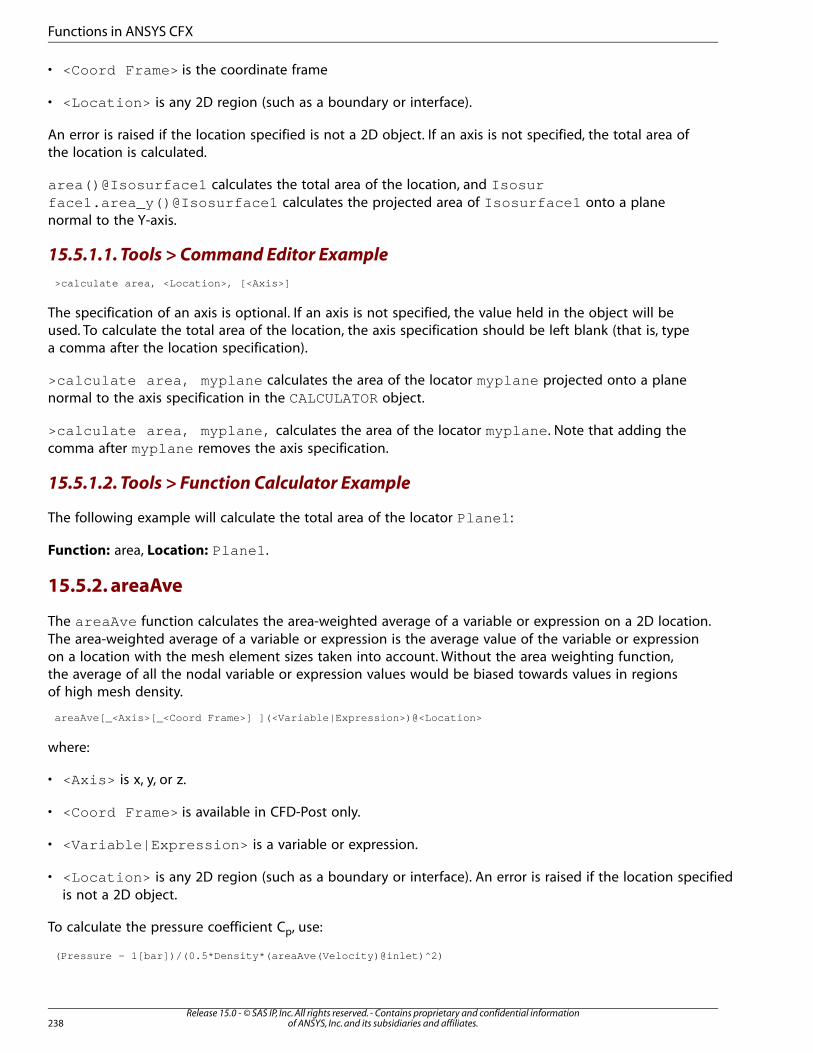
• <Coord Frame> is the coordinate frame
• <Location> is any 2D region (such as a boundary or interface).
An error is raised if the location specified is not a 2D object. If an axis is not specified, the total area ofthe location is calculated.
area()@Isosurface1 calculates the total area of the location, and Isosurface1.area_y()@Isosurface1 calculates the projected area of Isosurface1 onto a planenormal to the Y-axis.
15.5.1.1. Tools > Command Editor Example
>calculate area, <Location>, [<Axis>]
The specification of an axis is optional. If an axis is not specified, the value held in the object will beused. To calculate the total area of the location, the axis specification should be left blank (that is, typea comma after the location specification).
>calculate area, myplane calculates the area of the locator myplane projected onto a planenormal to the axis specification in the CALCULATOR object.
>calculate area, myplane, calculates the area of the locator myplane . Note that adding thecomma after myplane removes the axis specification.
15.5.1.2. Tools > Function Calculator Example
The following example will calculate the total area of the locator Plane1 :
Function: area, Location: Plane1 .
15.5.2. areaAve
The areaAve function calculates the area-weighted average of a variable or expression on a 2D location.The area-weighted average of a variable or expression is the average value of the variable or expressionon a location with the mesh element sizes taken into account. Without the area weighting function,the average of all the nodal variable or expression values would be biased towards values in regionsof high mesh density.
areaAve[_<Axis>[_<Coord Frame>] ](<Variable|Expression>)@<Location>
where:
• <Axis> is x, y, or z.
• <Coord Frame> is available in CFD-Post only.
• <Variable|Expression> is a variable or expression.
• <Location> is any 2D region (such as a boundary or interface). An error is raised if the location specifiedis not a 2D object.
To calculate the pressure coefficient Cp, use:
(Pressure - 1[bar])/(0.5*Density*(areaAve(Velocity)@inlet)^2)
Release 15.0 - © SAS IP, Inc. All rights reserved. - Contains proprietary and confidential informationof ANSYS, Inc. and its subsidiaries and affiliates.238
Functions in ANSYS CFX
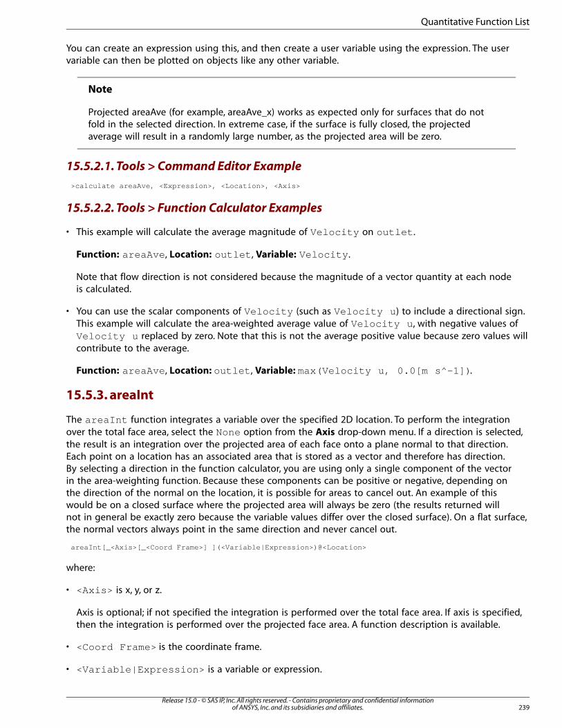
You can create an expression using this, and then create a user variable using the expression. The uservariable can then be plotted on objects like any other variable.
Note
Projected areaAve (for example, areaAve_x) works as expected only for surfaces that do notfold in the selected direction. In extreme case, if the surface is fully closed, the projectedaverage will result in a randomly large number, as the projected area will be zero.
15.5.2.1. Tools > Command Editor Example
>calculate areaAve, <Expression>, <Location>, <Axis>
15.5.2.2. Tools > Function Calculator Examples
• This example will calculate the average magnitude of Velocity on outlet .
Function: areaAve , Location: outlet , Variable: Velocity .
Note that flow direction is not considered because the magnitude of a vector quantity at each nodeis calculated.
• You can use the scalar components of Velocity (such as Velocity u ) to include a directional sign.This example will calculate the area-weighted average value of Velocity u , with negative values ofVelocity u replaced by zero. Note that this is not the average positive value because zero values willcontribute to the average.
Function: areaAve , Location: outlet , Variable: max(Velocity u, 0.0[m s^-1]) .
15.5.3. areaInt
The areaInt function integrates a variable over the specified 2D location. To perform the integrationover the total face area, select the None option from the Axis drop-down menu. If a direction is selected,the result is an integration over the projected area of each face onto a plane normal to that direction.Each point on a location has an associated area that is stored as a vector and therefore has direction.By selecting a direction in the function calculator, you are using only a single component of the vectorin the area-weighting function. Because these components can be positive or negative, depending onthe direction of the normal on the location, it is possible for areas to cancel out. An example of thiswould be on a closed surface where the projected area will always be zero (the results returned willnot in general be exactly zero because the variable values differ over the closed surface). On a flat surface,the normal vectors always point in the same direction and never cancel out.
areaInt[_<Axis>[_<Coord Frame>] ](<Variable|Expression>)@<Location>
where:
• <Axis> is x, y, or z.
Axis is optional; if not specified the integration is performed over the total face area. If axis is specified,then the integration is performed over the projected face area. A function description is available.
• <Coord Frame> is the coordinate frame.
• <Variable|Expression> is a variable or expression.
239Release 15.0 - © SAS IP, Inc. All rights reserved. - Contains proprietary and confidential information
of ANSYS, Inc. and its subsidiaries and affiliates.
Quantitative Function List
• <Location> is any 2D region (such as a boundary or interface). An error is raised if the location specifiedis not a 2D object.
areaInt_y_Frame2(Pressure)@boundary1 calculates the pressure force acting in the y-directionof the coordinate frame Frame2 on the locator boundary1 . This differs from a calculation using theforce function, which calculates the total force on a wall boundary (that is, viscous forces on theboundary are included).
15.5.3.1. Tools > Command Editor Example
>calculate areaInt, <Expression>, <Location>, [<Axis>]
Axis is optional. If it is not specified, the value held in the object will be used. To perform the integrationover the total face area, the axis specification should be blank (that is, type a comma after the locationname). A function description is available in areaInt (p. 239).
15.5.3.2. Tools > Function Calculator Examples
• This example integrates Pressure over Plane 1 . The returned result is the total pressure force actingon Plane 1 . The magnitude of each area vector is used and so the direction of the vectors is not con-sidered.
Function: areaInt , Location: Plane 1 , Variable: Pressure , Direction: None
• This example integrates Pressure over the projected area of Plane 1 onto a plane normal to the X-axis. The result is the pressure force acting in the X-direction on Plane 1 . This differs slightly from usingthe force function to calculate the X-directional force on Plane 1 . The force function includes forcesdue to the advection of momentum when calculating the force on an internal arbitrary plane or a non-wall boundary (inlets, etc.).
Function: areaInt, Location: Plane 1 , Variable: Pressure , Direction: Global X .
15.5.4. ave
The ave function calculates the arithmetic average of a variable or expression on the specified location.
Note
CFD-Post and CFX-Solver may compute slightly different average values due to differencesin how the average is computed:
• CFD-Post computes the arithmetically averaged vertex value for the location. Specifically, theaverage is computed by summing the vertex values and then dividing by the number of vertices.
• CFX-Solver computes the arithmetically averaged face value for the location. Specifically, theaverage is computed by summing the face values and then dividing by the number of faces.The value for a particular face is computed by arithmetically averaging the vertex values of theface.
Results will be biased towards areas of high nodal density on the location. To obtain a mesh independentresult, you should use the lengthAve , areaAve , volumeAve or massFlowAve functions.
ave(<Variable|Expression>)@<Location>
Release 15.0 - © SAS IP, Inc. All rights reserved. - Contains proprietary and confidential informationof ANSYS, Inc. and its subsidiaries and affiliates.240
Functions in ANSYS CFX
where:
• <Variable|Expression> is a variable or expression.
• <Location> is any 3D region (such as a domain or subdomain).
The ave function can be used on point, 1D, 2D, and 3D locations.
ave(Yplus)@Default calculates the mean Yplus values from each node on the default walls.
15.5.4.1. Tools > Command Editor Example
>calculate ave, <Variable|Expression>, <Location>
Note
To obtain a mesh-independent result, you should use the lengthAve , areaAve , volumeAveor massFlowAve functions.
The average of a vector value is calculated as an average of its magnitudes, not the magnitude ofcomponent averages. As an example, for velocity:
(15.1)= +�
� �
���
� �
where
(15.2)= + +� � � �� � � � ��
�
�
�
�
�
15.5.4.2. Tools > Function Calculator Example
This example calculates the mean temperature at all nodes in the selected domain.
Function: ave , Location: MainDomain , Variable: Temperature .
15.5.5. count
The count function returns the number of nodes on the specified location.
count()@<Location>
where:
• <Location> is valid for point, 1D, 2D, and 3D locations.
count()@Polyline1 returns the number of points on the specified polyline locator.
15.5.5.1. Tools > Command Editor Example
>calculate count, <Location>
15.5.5.2. Tools > Function Calculator Example
This example returns the number of nodes in the specified domain.
241Release 15.0 - © SAS IP, Inc. All rights reserved. - Contains proprietary and confidential information
of ANSYS, Inc. and its subsidiaries and affiliates.
Quantitative Function List
Function: count , Location: MainDomain .
15.5.6. countTrue
The countTrue function returns the number of mesh nodes on the specified region that evaluate to“true”, where true means greater than or equal to 0.5. The countTrue function is valid for 1D, 2D, and3D locations.
countTrue(<Expression>)@<Location>
where <Expression> is:
• In CFD-Post, an expression that contains the logical operators =, >, <, <=, or >=.
• In CFX-Solver, an Additional Variable that you define. For example:
TemperatureLE = Temperature > 300[K]
countTrue(TemperatureLE)@Polyline1 returns the number of nodes on the specified polylinelocator that evaluate to true.
15.5.6.1. Tools > Command Editor Examples
In CFD-Post:
>calculate countTrue(Temperature > 300[K]), Domain1
In CFX-Solver:
>calculate countTrue(TemperatureLE), Domain1
15.5.6.2. Tools > Function Calculator Example
This example returns the number of nodes that evaluate to “true” in the specified domain.
Function: countTrue , Location: MainDomain , Expression: Temperature > 300[K] .
15.5.7. force
This function returns the force exerted by the fluid on the specified 2D locator in the specified direction.
[<Phase>.]force[_<Axis>[_<Coord Frame>] ]()@<Location>
where:
• [<Phase>.] is an optional prefix that is not required for single-phase flows. For details, see CEL Functionswith Multiphase Flow (p. 232).
• <Axis> is x, y, or z
• <Coord Frame> is the coordinate frame
• <Location> is any 2D region (such as a boundary or interface).
Force calculations on boundaries require additional momentum flow data.
Release 15.0 - © SAS IP, Inc. All rights reserved. - Contains proprietary and confidential informationof ANSYS, Inc. and its subsidiaries and affiliates.242
Functions in ANSYS CFX
Water at RTP.force_x()@wall1 returns the total force in the x-direction acting on wall1 dueto the fluid Water at RTP .
The force on a boundary is calculated using momentum flow data from the results file, if it is available.The result can be positive or negative, indicating the direction of the force. For non-boundary locators,an approximate force is always calculated.
CFD-Post calculates the approximate force as follows:
• If the locator is a wall boundary, the force is equal to the pressure force.
• For all other locators, the force is equal to the pressure force plus the mass flow force (due to the advectionof momentum).
• In all cases, if wall shear data exists in the results file, the viscous force is added to the calculated force.
The force function enables you to select the fluids to use when performing your calculation. Theresult returned is the force on the locator due to that fluid/those fluids. Because the pressure force isthe same at each node irrespective of the choice of fluids, the only difference is in the viscous forces(on wall boundaries) or the mass flow forces.
It is important to note that forces arising as a result of the reference pressure are not included in theforce calculation. You can include reference pressure effects in the force calculation in the CFX-Solverby setting the expert parameter include pref in forces = t .
When performing transient simulations with rotating reference frames, forces may be reported in eitherthe stationary frame or the rotating frame. The forces reported by the CFX-Solver out file are alwaysgiven in the rotating frame. The forces reported by CFD-Post are reported in the stationary frame if the‘Angular shift for Transient Rotating Domains’ option is active, as discussed in Angular Shift for TransientRotating Domains in the CFD-Post User's Guide.
15.5.7.1. Tools > Command Editor Example
>calculate force, <Location>, <Axis>, [<Phase>]
15.5.7.2. Tools > Function Calculator Examples
• This calculates the total force on the default wall boundaries in the x-direction. Pressure and viscous forcesare included.
Function: force , Location: Default , Direction: Global X , Phase: All Fluids .
• This calculates the forces on inlet1 due to pressure and the advection of momentum.
Function: force, Location: inlet1, Direction: Global X , Phase: Water at RTP .
15.5.8. forceNorm
Returns the per unit width force on a line in the direction of the specified axis. It is available only for apolyline created by intersecting a locator on a boundary. Momentum data must also be available. Themagnitude of the value returned can be thought of as the force in the specified direction on a polyline,if the polyline were 2D with a width of one unit.
[<Phase>.]forceNorm[_<Axis>[_<Coord Frame>] ]()@<Location>
where:
243Release 15.0 - © SAS IP, Inc. All rights reserved. - Contains proprietary and confidential information
of ANSYS, Inc. and its subsidiaries and affiliates.
Quantitative Function List
• [<Phase>.] is an optional prefix that is not required for single-phase flows. For details, see CEL Functionswith Multiphase Flow (p. 232).
• <Axis> is x, y, or z
• <Coord Frame> is available in CFD-Post only
• <Location> is any 1D location. An error will be raised if the location specified is not one-dimensional.
forceNorm_y()@Polyline1 calculates the per unit width force in the y-direction on the selectedpolyline.
15.5.8.1. Tools > Command Editor Example
>calculate forceNorm, <Location>, <Axis>, [<Phase>]
15.5.8.2. Tools > Function Calculator Example
The result from this calculation is force per unit width on Polyline1 in the x-direction.
Function: forceNorm , Location: Polyline1 , Direction: Global X , Phase: All Fluids .
15.5.9. inside
The inside CEL function is essentially a step function variable, defined to be unity within a subdomainand zero elsewhere. This is useful for describing different initial values or fluid properties in differentregions of the domain. It is similar to the CEL subdomain variable, but allows a specific 2D or 3D locationto be given. For example, 273 [K] * inside()@Subdomain 1 has a value of 273 [K] at pointsin Subdomain 1 and 0 [K] elsewhere. The location does not need to be a subdomain, but can be any2D or 3D named sub-region of the physical location on which the expression is evaluated. For immersedsolids simulations, the location can also be a specific immersed solid domain, and the inside functionwill be updated automatically at the beginning of each time step.
inside()@<Location>
where:
• <Location> is any 2D or 3D named sub-region of the physical location on which the expression isevaluated.
• <Location> can also be an immersed solid domain on which the expression is evaluated dynamically.
Note
The inside CEL function is not available in CFD-Post.
15.5.9.1. Tools > Command Editor Example
>calculate inside, <Location>
15.5.10. length
Computes the length of the specified line as the sum of the distances between the points making upthe line.
Release 15.0 - © SAS IP, Inc. All rights reserved. - Contains proprietary and confidential informationof ANSYS, Inc. and its subsidiaries and affiliates.244
Functions in ANSYS CFX
length()@<Location>
where:
• <Location> is any 1D location. Specifying a 2D location will not produce an error; the sum of the edgelengths from the elements in the locator will be returned.
length()@Polyline1 returns the length of the polyline.
15.5.10.1. Tools > Command Editor Example
>calculate length, <Location>
Note
While using this function in Power Syntax, the leading character is capitalized to avoid con-fusion with the Perl internal command “length”.
15.5.10.2. Tools > Function Calculator Example
This example calculates the length of a polyline.
Function: length , Location: Polyline1 .
15.5.11. lengthAve
Computes the length-based average of the variable or expression on the specified line. This is the 1Dequivalent of the areaAve function. The results is independent of the nodal distribution along theline because a weighting function assigns a higher weighting to areas of sparse nodal density.
lengthAve(<Variable|Expression>)@<Location>
where:
• <Variable|Expression> is a variable or expression.
• <Location> is any 1D or 2D location.
lengthAve(T)@Polyline1 calculates the average temperature on Polyline1 weighted by thedistance between each point (T is the system variable for temperature).
15.5.11.1. Tools > Command Editor Example
>calculate lengthAve, <Expression>, <Location>
15.5.11.2. Tools > Function Calculator Example
This calculates the average velocity on the location Polyline1 using a length-based weighting functionto account for the distribution of points along the line.
Function: lengthAve , Location: Polyline1 , Variable: Velocity .
245Release 15.0 - © SAS IP, Inc. All rights reserved. - Contains proprietary and confidential information
of ANSYS, Inc. and its subsidiaries and affiliates.
Quantitative Function List
15.5.12. lengthInt
Computes the length-based integral of the variable or expression on the specified line. This is the 1Dequivalent of the areaInt function.
lengthInt(<Variable|Expression>)@<Location>
where:
• <Variable|Expression> is a variable or expression.
• <Location> is any 1D location.
15.5.12.1. Tools > Command Editor Example
>calculate lengthInt, <Expression>, <Location>.
15.5.13. mass
mass()@<Location>
where:
• <Location> is any 3D region (such as a domain or subdomain).
15.5.14. massAve
massAve(<Variable|Expression>)@<Location>
where:
• <Variable|Expression> is a variable or expression.
• <Location> is any 3D region (such as a domain or subdomain).
15.5.15. massFlow
Computes the mass flow through the specified 2D location.
[<Phase>.]massFlow()@<Location>
where:
• [<Phase>.] is an optional prefix that is not required for single-phase flows. For details, see CEL Functionswith Multiphase Flow (p. 232).
• <Location> is any fluid surfaces (such as Inlets, Outlets, Openings and fluid-fluid interfaces).
Air at STP.massFlow()@DegassingOutlet calculates the mass flow of Air at STP throughthe selected location.
For boundary locators:
Release 15.0 - © SAS IP, Inc. All rights reserved. - Contains proprietary and confidential informationof ANSYS, Inc. and its subsidiaries and affiliates.246
Functions in ANSYS CFX
• The mass flow is calculated using mass flow data from the results file, if it is available1. Otherwise, an ap-proximate mass flow is calculated.
• For multiphase cases, the mass flow through a boundary on a GGI interface evaluated in CFD-Post is anapproximation to the 'exact' mass flow evaluated by the solver. This approximation vanishes as the meshis refined or as the volume fraction on the interface becomes uniform.
For non-boundary locators (that is, internal locators):
• If the locator is an edge based locator (such as a slice plane or isosurface), the domain mass flow datafrom the results file will be used.
• In all other cases, an approximate mass flow is calculated.
• There is a limitation with the massFlow function on isosurfaces and slice planes that cross non-matching(that is, not 1-to-1) periodic interfaces. In such cases, the computed mass flow may not be accurate. Toperform a more accurate mass flow calculation, the following expression can be used:
areaInt_x(Velocity u * Density)@myLoc + areaInt_y(Velocity v * Density)@myLoc + areaInt_z(Velocity w * Density)@myLoc
The massFlow function enables you to select the fluids to use when performing your calculation. Theresult returned is the mass flow of the selected fluids through the locator.
If a user specifies a boundary mass source, this mass source is not included in the massFlow calculator.This will affect all massFlow related calculations, such as massFlowInt().
15.5.15.1. Mass Flow Sign Convention
The mass flow through a surface is defined by − ⋅� where is the velocity vector and is thesurface normal vector. By convention, the surface normal at a domain boundary is directed out of thedomain. Therefore, the mass flow is positive at an inlet boundary with the velocity directed into thedomain. For planes and surfaces that cut through a domain, the normal of the plane or surface is de-termined by from the right-hand rule and the manner in which the plane or surface is constructed. Forexample, the surface normal for a Z-X plane has the same sense and direction as the Y-axis.
15.5.15.2. Tools > Command Editor Example
>calculate massFlow, <Location>, [<Phase>]
15.5.15.3. Tools > Function Calculator Example
This calculates the mass flow for all fluids in the domains through the location outlet2:
Function: massFlow , Location: outlet2 , Phase: All Fluids .
1The availability depends on the setting for Output Boundary Flows for the file (see Output Boundary Flows Check Box in the CFX-
Pre User's Guide for details).
In addition to this, mass flow information written to a backup file at time zero is not accurate. To calculate accurate mass flowfrom a backup file, use information from the backup file written after the first timestep/iteration of the run.
247Release 15.0 - © SAS IP, Inc. All rights reserved. - Contains proprietary and confidential information
of ANSYS, Inc. and its subsidiaries and affiliates.
Quantitative Function List
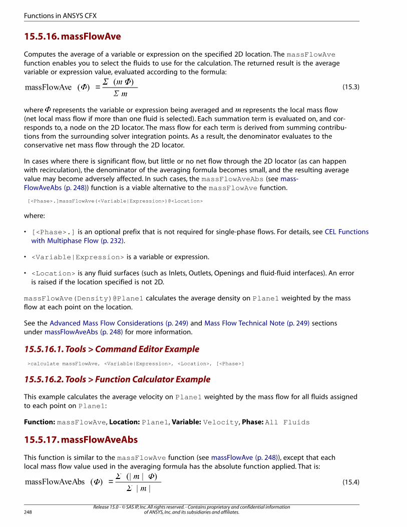
15.5.16. massFlowAve
Computes the average of a variable or expression on the specified 2D location. The massFlowAvefunction enables you to select the fluids to use for the calculation. The returned result is the averagevariable or expression value, evaluated according to the formula:
(15.3)=�� ��
� �
where � represents the variable or expression being averaged and � represents the local mass flow(net local mass flow if more than one fluid is selected). Each summation term is evaluated on, and cor-responds to, a node on the 2D locator. The mass flow for each term is derived from summing contribu-tions from the surrounding solver integration points. As a result, the denominator evaluates to theconservative net mass flow through the 2D locator.
In cases where there is significant flow, but little or no net flow through the 2D locator (as can happenwith recirculation), the denominator of the averaging formula becomes small, and the resulting averagevalue may become adversely affected. In such cases, the massFlowAveAbs (see mass-FlowAveAbs (p. 248)) function is a viable alternative to the massFlowAve function.
[<Phase>.]massFlowAve(<Variable|Expression>)@<Location>
where:
• [<Phase>.] is an optional prefix that is not required for single-phase flows. For details, see CEL Functionswith Multiphase Flow (p. 232).
• <Variable|Expression> is a variable or expression.
• <Location> is any fluid surfaces (such as Inlets, Outlets, Openings and fluid-fluid interfaces). An erroris raised if the location specified is not 2D.
massFlowAve(Density)@Plane1 calculates the average density on Plane1 weighted by the massflow at each point on the location.
See the Advanced Mass Flow Considerations (p. 249) and Mass Flow Technical Note (p. 249) sectionsunder massFlowAveAbs (p. 248) for more information.
15.5.16.1. Tools > Command Editor Example
>calculate massFlowAve, <Variable|Expression>, <Location>, [<Phase>]
15.5.16.2. Tools > Function Calculator Example
This example calculates the average velocity on Plane1 weighted by the mass flow for all fluids assignedto each point on Plane1 :
Function: massFlowAve , Location: Plane1 , Variable: Velocity , Phase: All Fluids
15.5.17. massFlowAveAbs
This function is similar to the massFlowAve function (see massFlowAve (p. 248)), except that eachlocal mass flow value used in the averaging formula has the absolute function applied. That is:
(15.4)=�� � �
� �
Release 15.0 - © SAS IP, Inc. All rights reserved. - Contains proprietary and confidential informationof ANSYS, Inc. and its subsidiaries and affiliates.248
Functions in ANSYS CFX
[<Phase>.]massFlowAveAbs(<Variable|Expression>)@<Location>
where:
• [<Phase>.] is an optional prefix that is not required for single-phase flows. For details, see CEL Functionswith Multiphase Flow (p. 232).
• <Variable|Expression> is a variable or expression.
• <Location> is any fluid surfaces (such as Inlets, Outlets, Openings and fluid-fluid interfaces). An erroris raised if the location specified is not 2D.
massFlowAve(Density)@Plane1 calculates the average density on Plane1 weighted by the massflow at each point on the location.
In cases where there is significant flow, but little or no net flow through the 2D locator (as can happenwith recirculation), the massFlowAveAbs function is a viable alternative to the massFlowAve function(see massFlowAve (p. 248)).
15.5.18. Advanced Mass Flow Considerations
Note that the massFlowAveAbs and massFlowAve functions provide the same result, and that thedenominator evaluates to the net mass flow through the 2D locator, only when all of the flow passesthrough the 2D locator in the same general direction (in other words, when there is no backflow). Ifthere is any backflow through the 2D locator, the denominator in the function for massFlowAveAbsevaluates to a value of greater magnitude than the conservative net mass flow through the 2D locator(although this is not necessarily harmful to the resulting average value).
The values of variables other than mass flow are stored at the mesh nodes and are applied to the loc-ator nodes by linear interpolation. For the mass flow variable, CFD-Post uses the integration point massflow data if it is available; otherwise, it will approximate mass flow values based on mesh node valuesof velocity (and density, if available).
15.5.19. Mass Flow Technical Note
When integration point mass flow data is stored, backflow through the 2D locator may occur as an ar-tifact of how the mass flow data is applied to the locator nodes, even though there may be no actualbackflow (as evidenced by a vector plot on the locator). The figure below illustrates how this may occur.
249Release 15.0 - © SAS IP, Inc. All rights reserved. - Contains proprietary and confidential information
of ANSYS, Inc. and its subsidiaries and affiliates.
Quantitative Function List
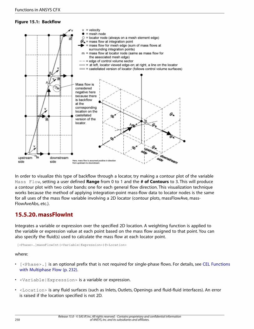
Figure 15.1: Backflow
In order to visualize this type of backflow through a locator, try making a contour plot of the variableMass Flow , setting a user defined Range from 0 to 1 and the # of Contours to 3. This will producea contour plot with two color bands: one for each general flow direction. This visualization techniqueworks because the method of applying integration-point mass-flow data to locator nodes is the samefor all uses of the mass flow variable involving a 2D locator (contour plots, massFlowAve, mass-FlowAveAbs, etc.).
15.5.20. massFlowInt
Integrates a variable or expression over the specified 2D location. A weighting function is applied tothe variable or expression value at each point based on the mass flow assigned to that point. You canalso specify the fluid(s) used to calculate the mass flow at each locator point.
[<Phase>.]massFlowInt(<Variable|Expression>)@<Location>
where:
• [<Phase>.] is an optional prefix that is not required for single-phase flows. For details, see CEL Functionswith Multiphase Flow (p. 232).
• <Variable|Expression> is a variable or expression.
• <Location> is any fluid surfaces (such as Inlets, Outlets, Openings and fluid-fluid interfaces). An erroris raised if the location specified is not 2D.
Release 15.0 - © SAS IP, Inc. All rights reserved. - Contains proprietary and confidential informationof ANSYS, Inc. and its subsidiaries and affiliates.250
Functions in ANSYS CFX
15.5.20.1. Tools > Command Editor Example
>calculate massFlowInt, <Variable|Expression>, <Location>, [<Phase>]
15.5.20.2. Tools > Function Calculator Example
This example integrates pressure over Plane1 . The result is the pressure force acting on Plane1 weightedby the mass flow assigned to each point on Plane1 :
Function: massFlowInt , Location: Plane1 , Variable: Pressure , Phase: All Fluids
15.5.21. massInt
The mass-weighted integration of a variable or expression within a domain or subdomain.
massInt(<Variable|Expression>)@<Location>
where:
• <Variable|Expression> is a variable or expression.
• <Location> is any 3D region (such as a domain or subdomain).
15.5.22. maxVal
Returns the maximum value of the specified variable or expression on the specified locator. You shouldcreate a user variable if you want to find the maximum value of an expression.
maxVal(<Variable|Expression>)@<Location>
where:
• <Variable|Expression> is a variable or expression.
• <Location> is, in the context of CFX-Solver, a 2D region or 3D region (such as a domain or subdomain)or, in the context of CFD-Post, a Point object or a 1D, 2D, or 3D locator.
15.5.22.1. Tools > Command Editor Example
>calculate maxVal, <Variable|Expression>, <Location>
15.5.22.2. Tools > Function Calculator Example
This will return the maximum Yplus value on the default wall boundaries:
Function: maxVal , Location: Default , Variable: Yplus
15.5.23. minVal
Returns the minimum value of the specified variable or expression on the specified locator. You shouldcreate a user variable if you want to find the minimum value of an expression.
minVal(<Variable|Expression>)@<Location>
where:
• <Variable|Expression> is a variable or expression.
251Release 15.0 - © SAS IP, Inc. All rights reserved. - Contains proprietary and confidential information
of ANSYS, Inc. and its subsidiaries and affiliates.
Quantitative Function List
• <Location> is, in the context of CFX-Solver, a 2D region or 3D region (such as a domain or subdomain)or, in the context of CFD-Post, a Point object or a 1D, 2D, or 3D locator.
15.5.23.1. Tools > Command Editor Example
>calculate minVal, <Variable|Expression>, <Location>
15.5.23.2. Tools > Function Calculator Example
These settings will return the minimum temperature in the domain:
Function: minVal , Location: MainDomain , Variable: Temperature
15.5.24. probe
Returns the value of the specified variable or expression on the specified Point object.
probe(<Variable|Expression>)@<Location>
where:
• <Variable|Expression> is a variable or expression.
• <Location> is any point object (such as a Source Point or Cartesian Monitor Point).
Important
This calculation should be performed only for point locators described by single points. In-correct solutions will be produced for multiple point locators.
15.5.24.1. Tools > Command Editor Example
>calculate probe, <Expression>, <Location>
15.5.24.2. Tools > Function Calculator Example
This example returns the density value at Point1 :
Function: probe , Location: Point1 , Variable: Density
15.5.25. rbstate
Returns the value of the specified rigid body state variable, or axis component thereof, on the specified:
• Rigid Body object (for a standard rigid body definition), or
• Immersed Solid domain that is governed by a rigid body solution.
The rigid body state variables are:
• Position
• Linear Velocity
• Linear Acceleration
Release 15.0 - © SAS IP, Inc. All rights reserved. - Contains proprietary and confidential informationof ANSYS, Inc. and its subsidiaries and affiliates.252
Functions in ANSYS CFX
• Euler Angle
• Angular Velocity
• Angular Acceleration
Syntax:
rbstate(<rbvar>[<Axis>])@<Location>
where:
• <rbvar> is a rigid body state variable.
• <Axis> is X, Y, or Z.
For the Euler Angle rigid body state variable, an axis must be specified. For all of the other rigidbody state variables, the axis is optional. If you do not specify an axis, the magnitude of the vectoris returned. For example, if the variable is Position and you do not specify an axis, the distancefrom the origin will be returned.
• <Location> is any rigid body object or any immersed solid domain that is governed by a rigid bodysolution.
Results are given with respect to the global coordinate frame (Coord 0).
15.5.25.1. Expressions Details View Example
rbstate(Linear Velocity Z)@Buoy
15.5.26. rmsAve
The rmsAve function calculates the RMS average of a variable or expression on the specified location.
• CFX-Solver computes the RMS average of the vertex values for a 3D location.
• CFX-Solver computes the RMS average of the face values for a 2D location. The value for a particular faceis computed by arithmetically averaging the vertex values of the face.
rmsAve(<Variable|Expression>)@<Location>
where:
• <Variable|Expression> is a variable or expression.
• <Location> is a 2D region or 3D region (such as a domain or subdomain).
15.5.27. sum
The sum function calculates the sum of a variable or expression on the specified location.
Note
CFD-Post and CFX-Solver compute the sum in different ways:
• CFD-Post computes the sum of the vertex values for the location.
253Release 15.0 - © SAS IP, Inc. All rights reserved. - Contains proprietary and confidential information
of ANSYS, Inc. and its subsidiaries and affiliates.
Quantitative Function List

• CFX-Solver computes the sum of the vertex values for a 3D location.
• CFX-Solver computes the sum of the face values for a 2D location. The value for a particularface is computed by arithmetically averaging the vertex values of the face.
sum(<Variable|Expression>)@<Location>
where:
• <Variable|Expression> is a variable or expression.
• <Location> is, in the context of CFX-Solver, a 2D region or 3D region (such as a domain or subdomain)or, in the context of CFD-Post, a Point object or a 1D, 2D, or 3D locator.
15.5.27.1. Tools > Command Editor Example
>calculate sum, <Variable|Expression>, <Location>
15.5.27.2. Tools > Function Calculator Example
This example returns the sum of the finite volumes assigned to each node in the location SubDomain1 .In this case, this sums to the volume of the subdomain:
Function: sum, Location: SubDomain1 , Variable: Volume of Finite Volume
15.5.28. torque
Returns the torque on a 2D locator about the specified axis. The force calculated during evaluation ofthe torque function has the same behavior as the force function. For details, see force (p. 242). You canselect the fluids involved in the calculation.
[<Phase>.]torque_[<Axis>[_<Coord Frame>] ]()@<Location>
where:
• [<Phase>.] is an optional prefix that is not required for single-phase flows. For details, see CEL Functionswith Multiphase Flow (p. 232).
• <Axis> is x, y, or z
• <Coord Frame>
• <Location> is any 2D region (such as a wall). If the location specified is not 2D, an error is raised.
15.5.28.1. Tools > Command Editor Example
>calculate torque, <Location>, <Axis>, [<Phase>]
15.5.28.2. Tools > Function Calculator Example
This example calculates the torque on Plane1 about the z-axis due to all fluids in the domain.
Function: torque , Location: Plane1 , Axis: Global Z , Phase: All Fluids
Release 15.0 - © SAS IP, Inc. All rights reserved. - Contains proprietary and confidential informationof ANSYS, Inc. and its subsidiaries and affiliates.254
Functions in ANSYS CFX
15.5.29. volume
Calculates the volume of a 3D location.
volume()@<Location>
where:
• <Location> is any 3D region (such as a domain or subdomain). An error is raised if the location specifiedis not a 3D object. For details, see volume (p. 255).
15.5.29.1. Tools > Command Editor Example
>calculate volume, <Location>
15.5.29.2. Tools > Function Calculator Example
This example returns the sum of the volumes of each mesh element included in the location Volume1 .
Function: volume , Location: Volume1
15.5.30. volumeAve
Calculates the volume-weighted average of a variable or expression on a 3D location. This is the 3Dequivalent of the areaAve function. The volume-weighted average is the average value on a locationweighted by the volume assigned to each vertex on a location. Without the volume weighting function,the average of all the nodal values would be biased towards values in regions of high mesh density.The following example demonstrates use of the function.
volumeAve(<Variable|Expression>)@<Location>
where:
• <Variable|Expression> is a variable or expression.
• <Location> is any 3D region (such as a domain or subdomain).
15.5.30.1. Tools > Command Editor Example
>calculate volumeAve, <Variable|Expression>, <Location>
15.5.30.2. Tools > Function Calculator Example
This example calculates the volume-weighted average value of density in the region enclosed by thelocation Volume1 :
Function: volumeAve , Location: Volume1 , Variable: Density
15.5.31. volumeInt
Integrates the specified variable or expression over the volume location. This is the 3D equivalent ofthe areaInt function.
volumeInt(<Variable|Expression>)@<Location>
where:
255Release 15.0 - © SAS IP, Inc. All rights reserved. - Contains proprietary and confidential information
of ANSYS, Inc. and its subsidiaries and affiliates.
Quantitative Function List
• <Variable|Expression> is a variable or expression.
• <Location> is any 3D region (such as a domain or subdomain). An error is raised if the location specifiedis not a 3D object.
For example, volumeInt(Density)@StaticMixer will calculate the total fluid mass in the domainStaticMixer .
Note
Because the Density variable represents the average density during the timestep rather thanthe density at the end of the timestep, the volumeInt(Density) does not accuratelygive the mass of fluid at the end of a timestep. Use the mass() function instead.
15.5.31.1. Tools > Command Editor Example
>calculate volumeInt, <Variable|Expression>, <Location>
15.5.31.2. Tools > Function Calculator Example
This example calculates the integral of density (the total mass) in Volume1 .
Function: volumeInt , Location: Volume1 , Variable: Density
Release 15.0 - © SAS IP, Inc. All rights reserved. - Contains proprietary and confidential informationof ANSYS, Inc. and its subsidiaries and affiliates.256
Functions in ANSYS CFX
Chapter 16: Variables in ANSYS CFX
This chapter describes the variables available in ANSYS CFX:16.1. Hybrid and Conservative Variable Values16.2. List of Field Variables16.3. Particle Variables Generated by the Solver16.4. Miscellaneous Variables
16.1. Hybrid and Conservative Variable Values
The CFX-Solver calculates the solution to your CFD problem using polyhedral finite volumes surroundingthe vertices of the underlying mesh elements (hexahedrons, tetrahedrons, prisms, pyramids). Analyticalsolutions to the Navier-Stokes equations exist for only the simplest of flows under ideal conditions. Toobtain solutions for real flows, a numerical approach must be adopted whereby the equations are re-placed by algebraic approximations that may be solved using a numerical method.
The solution values on the boundary vertices, called conservative values, are the values obtained fromsolving the conservation equations for the boundary control volumes. These values are not necessarilythe same as the specified boundary condition values, although the specified boundary value is used toclose boundary fluxes for the boundary control volume. For example, on a no-slip wall, the wall velocityis used to compute the viscous force for the boundary face of the boundary control volume, but theresulting control volume equation solution will not necessarily be the wall velocity. The conservativevalues are representative of the boundary control volume, not the boundary itself. For visualizationpurposes, it is often useful to view the specified boundary condition value for the boundary verticesrather than the conservative values. This is especially true when the value of a conservative solutionvariable (such as pressure or temperature, for instance) is specified at a particular boundary condition.The specified boundary values are called hybrid values. CFD-Post uses hybrid values by default for mostvariables. Hybrid values are obtained by overwriting the conservative results on the boundary nodesproduced by the CFX-Solver with values based on the specified boundary conditions. This ensures, forexample, that the velocity is displayed as zero on no-slip walls. For quantitative calculations, the conser-vative values should normally be used because they are consistent with the discrete solutions obtainedby the solver. If you want to use these values in CFD-Post, you can select them from the Variables
Editor dialog box as described above. By default, CFD-Post uses conservative values when the Calculate
command is used.
The difference between hybrid and conservative values at wall boundaries can be demonstrated usingthe following figure:
257Release 15.0 - © SAS IP, Inc. All rights reserved. - Contains proprietary and confidential information
of ANSYS, Inc. and its subsidiaries and affiliates.

Using velocity as an example, the velocity value calculated at a mesh node is based upon the ‘average’in the control volume surrounding that node. For calculation purposes, the entire control volume isthen assumed to possess that velocity. At a boundary node, its surrounding control volume includesan area in the bulk of the fluid (this area is highlighted around the boundary node marked 1). Hence,the conservative velocity calculated at the wall node is not zero, but an ‘average’ over the controlvolume adjacent to the boundary. At a wall boundary node the difference between conservative andhybrid values can be illustrated by considering the case of the mass flow rate through the wall-adjacentcontrol volume. If a zero velocity was enforced at the boundary node, then this would produce zeromass flow through the control volume, which is clearly not correct.
16.1.1. Solid-Fluid Interface Variable Values
16.1.1.1. Conservative Values at 1:1 Interface
At a solid-fluid 1:1 interface, duplicate nodes exist. The conservative value for the solid-side node is thevariable values averaged over the half on the control volume that lies inside the solid. The conservativevalue for the fluid-side node is the variable values averaged over the half of the control volume thatlies in the fluid.
Consider the example of heat transfer from a hot solid to a cool fluid when advection dominates withinthe fluid. If you create a plot across the solid-fluid interface using conservative values of temperature,then you will see a sharp change in temperature across the interface. This is because values are inter-polated from the interface into the bulk of the solid domain using the value for the solid-side node atthe interface, while values are interpolated from the interface into the bulk of the fluid domain usingthe value for the fluid-side node at the interface. This results in a temperature discontinuity at the inter-face.
16.1.1.2. Hybrid Values at 1:1 Interface
When creating plots using hybrid variable values (the default in CFD-Post), the 1:1 interface is singlevalued and takes the solid-side conservative value. You can therefore expect to see the same plotwithin the solid, but the temperature profile between the interface and the first node in the fluid inter-polates between the solid-side interface value and the first fluid node value. In this case, a discontinuitydoes not exist because all nodes are single valued.
Conservative values should be used for all quantitative calculations.
Release 15.0 - © SAS IP, Inc. All rights reserved. - Contains proprietary and confidential informationof ANSYS, Inc. and its subsidiaries and affiliates.258
Variables in ANSYS CFX
16.1.1.3. Conservative Values on a GGI Interface
At a GGI interface, the CFX Solver calculates both fluid-side and solid-side temperatures based on heatflux conservation. These values are representative of the temperature within the half-control volumesaround the vertices on the interface. The fluid-side and solid-side temperatures are generally not equal.As a result, a plot of conservative values of temperature will generally show a discontinuity across aGGI interface.
16.1.1.4. Hybrid Values on a GGI Interface
At a GGI interface, the CFX Solver calculates a "surface temperature" based on a flux-conservationequation for the 'control surfaces' that lie between the fluid side and the solid side. The surface temper-ature is usually between the fluid-side and solid-side temperatures. Hybrid values of temperature on aGGI interface are set equal to the surface temperature. As a result, there is no discontinuity in hybridvalues of temperature across a GGI interface.
16.2. List of Field Variables
This section contains a list of field variables that you may have defined in CFX-Pre or that are availablefor viewing in CFD-Post and exporting to other files. Many variables are relevant only for specificphysical models.
The information given in this section includes:
• Long Variable Name: The name that you see in the user interface.
• Short Variable Name: The name that must be used in CEL expressions.
• Units: The default units for the variable. An empty entry [ ] indicates a dimensionless variable.
Note
The entries in the Units columns are SI but could as easily be any other system of units.
• In the Availability column:
– A number represents the user level (1 indicates that the variable appears in default lists, 2 and 3 indicate
that the variable appears in extended lists that you see when you click ). This number is useful when
using the CFX Export facility. For details, see File Export Utility in the CFX-Solver Manager User's Guide.Note that the CFX-Solver may sometimes override the user-level setting depending on the physics ofthe problem. In these cases, the User Level may be different from that shown in the tables that follow.
– Boundary (B): A B in this column indicates that the variable contains only non-zero values on theboundary of the model. See Boundary-Value-Only Variables in the CFD-Post User's Guide for more details.
Boundary-Value-Only Variables in the CFD-Post User's Guide describes the useful things that youcan do with variables that are defined only on the boundaries of the model.
– A indicates the variable is available for mesh adaption
– C indicates the variable is available in CEL
259Release 15.0 - © SAS IP, Inc. All rights reserved. - Contains proprietary and confidential information
of ANSYS, Inc. and its subsidiaries and affiliates.
List of Field Variables
– DT indicates the variable is available for data transfer to ANSYS
– M indicates the variable is available for monitoring
– P indicates the variable is available for particle user-routine argument lists
– PR indicates the variable is available for particle results
– R indicates the variable is available to be output to the results, transient results, and backup files
– RA indicates the variable is available for radiation results
– TS indicates the variable is available for transient statistics
• Definition: Defines the variable.
This is not a complete list of variables. Information on obtaining details on all variables is available inRULES and VARIABLES Files in the CFX-Solver Manager User's Guide.
Note
Variables with names shown in bold text are not output to CFD-Post. However, some ofthese variables can be output to CFD-Post by selecting them from the Extra Output Variables
List on the Results tab of the Solver > Output Control details view of CFX-Pre.
16.2.1. Common Variables Relevant for Most CFD Calculations
The following table contains a list of variables (with both long and short variable names) that can beused when working with CFD calculations. For an explanation of the column headings, see List of FieldVariables (p. 259).
DefinitionAvailabil-
ity
UnitsShort
Vari-
able
Name
Long
Variable
Name
Mass per unit volume.1[kgm^-3]
dens-ity
Density
Note that for fixed compos-ition, variable composition,
A, C, M,P, R, TS
and reacting mixtures,when density is governedby the Ideal Mixtureoption, the density is de-termined by a mass-frac-tion-weighted harmonicaverage:
+ + … + =�
�
�
�
�
� �
��
�
�
�
�
� ���
Release 15.0 - © SAS IP, Inc. All rights reserved. - Contains proprietary and confidential informationof ANSYS, Inc. and its subsidiaries and affiliates.260
Variables in ANSYS CFX
DefinitionAvailabil-
ity
UnitsShort
Vari-
able
Name
Long
Variable
Name
Dynamic viscosity (�), alsocalled absolute viscosity, is
2
A, C, M,P, R, TS
[kg m^-1 s^-1]
viscos-ity
DynamicViscosity
a measure of the resistanceof a fluid to shearingforces, and appears in themomentum equations. Us-ing an expression to setthe dynamic viscosity ispossible. For details, seeNon-Newtonian Flow inthe CFX-Solver Modeling
Guide.
Velocity vector.1[ms^-1]
velVelocitya
A, C, M,P, R, TS
Components of velocity.1[ms^-1]
u
v
w
Velocityu
Velocityv
A, C, M,P, R, TS
Velocityw
Both Pressure andTotal Pressure are
1
A, C, M,P, R, TS
[kg m^-1 s^-2]
pPressure
measured relative to thereference pressure that youspecified on the Domains
panel in CFX-Pre. Addition-ally, Pressure is the totalnormal stress, whichmeans that when using thek-e turbulence model,Pressure is the thermo-dynamic pressure plus theturbulent normal stress.Static Pressure is thethermodynamic pressure,in most cases this is thesame as Pressure . Fordetails, see Modified Pres-sure in the CFX-Solver The-
ory Guide.
CFX solves for the relativeStatic Pressure
3[kg m^-1 s^-2]
pstatStaticPressure
261Release 15.0 - © SAS IP, Inc. All rights reserved. - Contains proprietary and confidential information
of ANSYS, Inc. and its subsidiaries and affiliates.
List of Field Variables
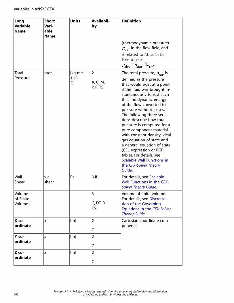
DefinitionAvailabil-
ity
UnitsShort
Vari-
able
Name
Long
Variable
Name
(thermodynamic pressure)�����
in the flow field, and
is related to AbsolutePressure
= +� � ���� ���� �
.
The total pressure, � �
, is
defined as the pressure
2
A, C, M,P, R, TS
[kg m^-1 s^-2]
ptotTotalPressure
that would exist at a pointif the fluid was brought in-stantaneously to rest suchthat the dynamic energyof the flow converted topressure without losses.The following three sec-tions describe how totalpressure is computed for apure component materialwith constant density, idealgas equation of state anda general equation of state(CEL expression or RGPtable). For details, seeScalable Wall Functions inthe CFX-Solver Theory
Guide.
For details, see ScalableWall Functions in the CFX-
Solver Theory Guide.
3,BPawallshear
WallShear
Volume of finite volume.For details, see Discretiza-
3
C, DT, R,TS
Volumeof FiniteVolume tion of the Governing
Equations in the CFX-Solver
Theory Guide.
Cartesian coordinate com-ponents.
2
C
[m]xX co-
ordinate
2[m]yY co-
ordinateC
2[m]zZ co-
ordinateC
Release 15.0 - © SAS IP, Inc. All rights reserved. - Contains proprietary and confidential informationof ANSYS, Inc. and its subsidiaries and affiliates.262
Variables in ANSYS CFX
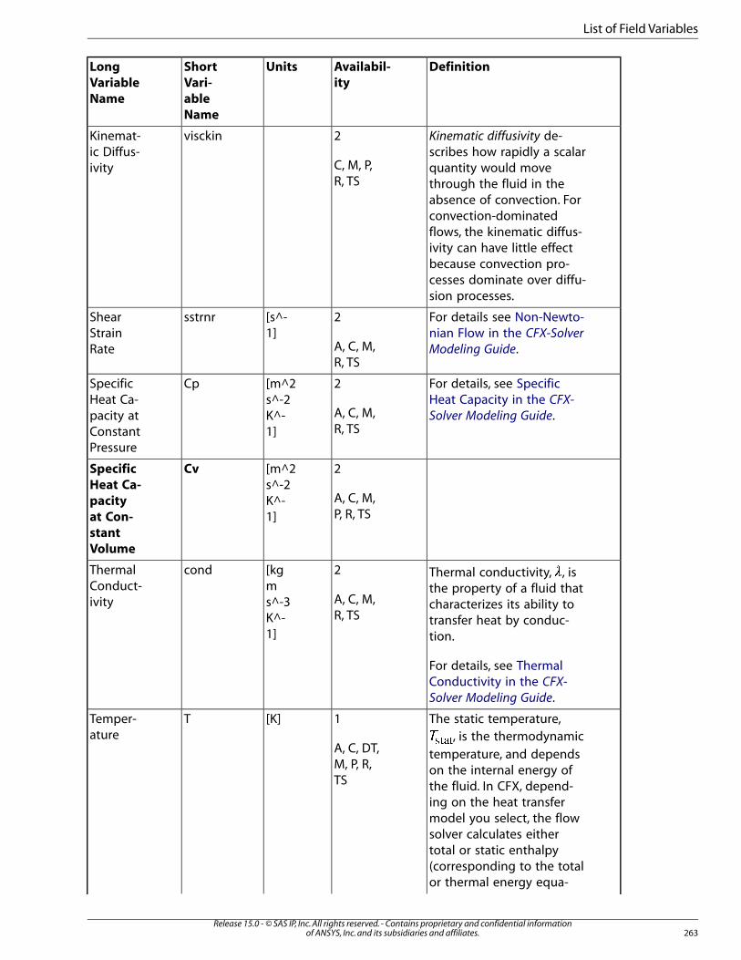
DefinitionAvailabil-
ity
UnitsShort
Vari-
able
Name
Long
Variable
Name
Kinematic diffusivity de-scribes how rapidly a scalar
2
C, M, P,R, TS
visckinKinemat-ic Diffus-ivity quantity would move
through the fluid in theabsence of convection. Forconvection-dominatedflows, the kinematic diffus-ivity can have little effectbecause convection pro-cesses dominate over diffu-sion processes.
For details see Non-Newto-nian Flow in the CFX-Solver
Modeling Guide.
2
A, C, M,R, TS
[s^-1]
sstrnrShearStrainRate
For details, see SpecificHeat Capacity in the CFX-
Solver Modeling Guide.
2
A, C, M,R, TS
[m^2s^-2K^-1]
CpSpecificHeat Ca-pacity atConstantPressure
2[m^2s^-2
CvSpecific
Heat Ca-A, C, M,P, R, TS
K^-1]
pacity
at Con-
stant
Volume
Thermal conductivity, �, isthe property of a fluid that
2
A, C, M,R, TS
[kgms^-3K^-1]
condThermalConduct-ivity characterizes its ability to
transfer heat by conduc-tion.
For details, see ThermalConductivity in the CFX-
Solver Modeling Guide.
The static temperature,�����, is the thermodynamic
1
A, C, DT,M, P, R,TS
[K]TTemper-ature
temperature, and dependson the internal energy ofthe fluid. In CFX, depend-ing on the heat transfermodel you select, the flowsolver calculates eithertotal or static enthalpy(corresponding to the totalor thermal energy equa-
263Release 15.0 - © SAS IP, Inc. All rights reserved. - Contains proprietary and confidential information
of ANSYS, Inc. and its subsidiaries and affiliates.
List of Field Variables
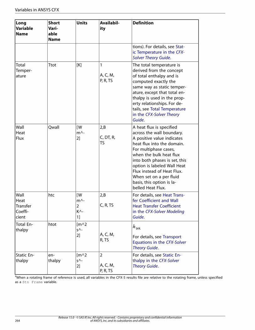
DefinitionAvailabil-
ity
UnitsShort
Vari-
able
Name
Long
Variable
Name
tions). For details, see Stat-ic Temperature in the CFX-
Solver Theory Guide.
The total temperature isderived from the concept
1
A, C, M,P, R, TS
[K]TtotTotalTemper-ature of total enthalpy and is
computed exactly thesame way as static temper-ature, except that total en-thalpy is used in the prop-erty relationships. For de-tails, see Total Temperaturein the CFX-Solver Theory
Guide.
A heat flux is specifiedacross the wall boundary.
2,B
C, DT, R,TS
[Wm^-2]
QwallWallHeatFlux A positive value indicates
heat flux into the domain.For multiphase cases,when the bulk heat fluxinto both phases is set, thisoption is labeled Wall HeatFlux instead of Heat Flux.When set on a per fluidbasis, this option is la-belled Heat Flux.
For details, see Heat Trans-fer Coefficient and Wall
2,B
C, R, TS
[Wm^-2
htcWallHeatTransfer Heat Transfer Coefficient
K^-1]
Coeffi-cient
in the CFX-Solver Modeling
Guide.
����
For details, see TransportEquations in the CFX-Solver
Theory Guide.
A, C, M,R, TS
[m^2s^-2]
htotTotal En-thalpy
For details, see Static En-thalpy in the CFX-Solver
Theory Guide.
2
A, C, M,P, R, TS
[m^2s^-2]
en-thalpy
Static En-thalpy
aWhen a rotating frame of reference is used, all variables in the CFX-5 results file are relative to the rotating frame, unless specifiedas a Stn Frame variable.
Release 15.0 - © SAS IP, Inc. All rights reserved. - Contains proprietary and confidential informationof ANSYS, Inc. and its subsidiaries and affiliates.264
Variables in ANSYS CFX
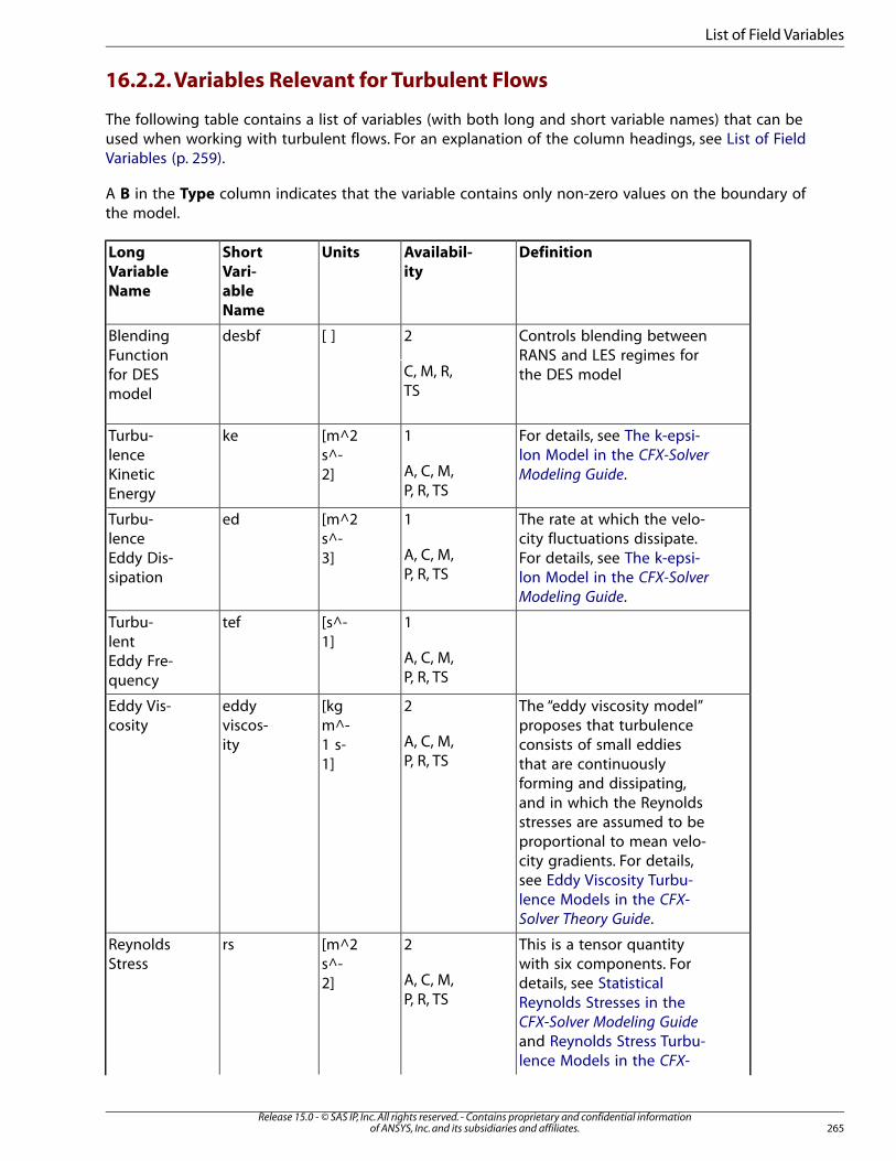
16.2.2. Variables Relevant for Turbulent Flows
The following table contains a list of variables (with both long and short variable names) that can beused when working with turbulent flows. For an explanation of the column headings, see List of FieldVariables (p. 259).
A B in the Type column indicates that the variable contains only non-zero values on the boundary ofthe model.
DefinitionAvailabil-
ity
UnitsShort
Vari-
able
Name
Long
Variable
Name
Controls blending betweenRANS and LES regimes forthe DES model
2
C, M, R,TS
[ ]desbfBlendingFunctionfor DESmodel
For details, see The k-epsi-lon Model in the CFX-Solver
Modeling Guide.
1
A, C, M,P, R, TS
[m^2s^-2]
keTurbu-lenceKineticEnergy
The rate at which the velo-city fluctuations dissipate.
1
A, C, M,P, R, TS
[m^2s^-3]
edTurbu-lenceEddy Dis-sipation
For details, see The k-epsi-lon Model in the CFX-Solver
Modeling Guide.
1[s^-1]
tefTurbu-lent
A, C, M,P, R, TS
Eddy Fre-quency
The “eddy viscosity model”proposes that turbulence
2
A, C, M,P, R, TS
[kgm^-1 s-1]
eddyviscos-ity
Eddy Vis-cosity
consists of small eddiesthat are continuouslyforming and dissipating,and in which the Reynoldsstresses are assumed to beproportional to mean velo-city gradients. For details,see Eddy Viscosity Turbu-lence Models in the CFX-
Solver Theory Guide.
This is a tensor quantitywith six components. For
2
A, C, M,P, R, TS
[m^2s^-2]
rsReynoldsStress
details, see StatisticalReynolds Stresses in theCFX-Solver Modeling Guide
and Reynolds Stress Turbu-lence Models in the CFX-
265Release 15.0 - © SAS IP, Inc. All rights reserved. - Contains proprietary and confidential information
of ANSYS, Inc. and its subsidiaries and affiliates.
List of Field Variables
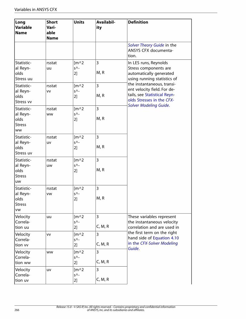
DefinitionAvailabil-
ity
UnitsShort
Vari-
able
Name
Long
Variable
Name
Solver Theory Guide in theANSYS CFX documenta-tion.
In LES runs, ReynoldsStress components are
3
M, R
[m^2s^-2]
rsstatuu
Statistic-al Reyn-oldsStress uu
automatically generatedusing running statistics ofthe instantaneous, transi-3[m^2
s^-2]
rsstatvv
Statistic-al Reyn-oldsStress vv
ent velocity field. For de-tails, see Statistical Reyn-olds Stresses in the CFX-
Solver Modeling Guide.
M, R
3[m^2s^-2]
rsstatww
Statistic-al Reyn-olds M, R
Stressww
3[m^2s^-2]
rsstatuv
Statistic-al Reyn-oldsStress uv
M, R
3[m^2s^-2]
rsstatuw
Statistic-al Reyn-olds M, R
Stressuw
3[m^2s^-2]
rsstatvw
Statistic-al Reyn-olds M, R
Stressvw
These variables representthe instantaneous velocity
3
C, M, R
[m^2s^-2]
uuVelocityCorrela-tion uu correlation and are used in
the first term on the right3[m^2s^-2]
vvVelocityCorrela-tion vv
hand side of Equation 4.10in the CFX-Solver Modeling
Guide.C, M, R
3[m^2s^-2]
wwVelocityCorrela-tion ww C, M, R
3[m^2s^-2]
uvVelocityCorrela-tion uv C, M, R
Release 15.0 - © SAS IP, Inc. All rights reserved. - Contains proprietary and confidential informationof ANSYS, Inc. and its subsidiaries and affiliates.266
Variables in ANSYS CFX
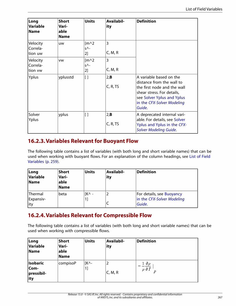
DefinitionAvailabil-
ity
UnitsShort
Vari-
able
Name
Long
Variable
Name
3[m^2s^-2]
uwVelocityCorrela-tion uw C, M, R
3[m^2s^-2]
vwVelocityCorrela-tion vw C, M, R
A variable based on thedistance from the wall to
2,B
C, R, TS
[ ]yplusstdYplus
the first node and the wallshear stress. For details,see Solver Yplus and Yplusin the CFX-Solver Modeling
Guide.
A deprecated internal vari-able. For details, see Solver
2,B
C, R, TS
[ ]yplusSolverYplus
Yplus and Yplus in the CFX-
Solver Modeling Guide.
16.2.3. Variables Relevant for Buoyant Flow
The following table contains a list of variables (with both long and short variable names) that can beused when working with buoyant flows. For an explanation of the column headings, see List of FieldVariables (p. 259).
DefinitionAvailabil-
ity
UnitsShort
Vari-
able
Name
Long
Variable
Name
For details, see Buoyancyin the CFX-Solver Modeling
Guide.
2
C
[K^ -1]
betaThermalExpansiv-ity
16.2.4. Variables Relevant for Compressible Flow
The following table contains a list of variables (with both long and short variable names) that can beused when working with compressible flows.
DefinitionAvailabil-
ity
UnitsShort
Vari-
able
Name
Long
Variable
Name
− ∂∂�
�
��
�2
C, M, R
[K^-1]
compisoPIsobaric
Com-
pressibil-
ity
267Release 15.0 - © SAS IP, Inc. All rights reserved. - Contains proprietary and confidential information
of ANSYS, Inc. and its subsidiaries and affiliates.
List of Field Variables
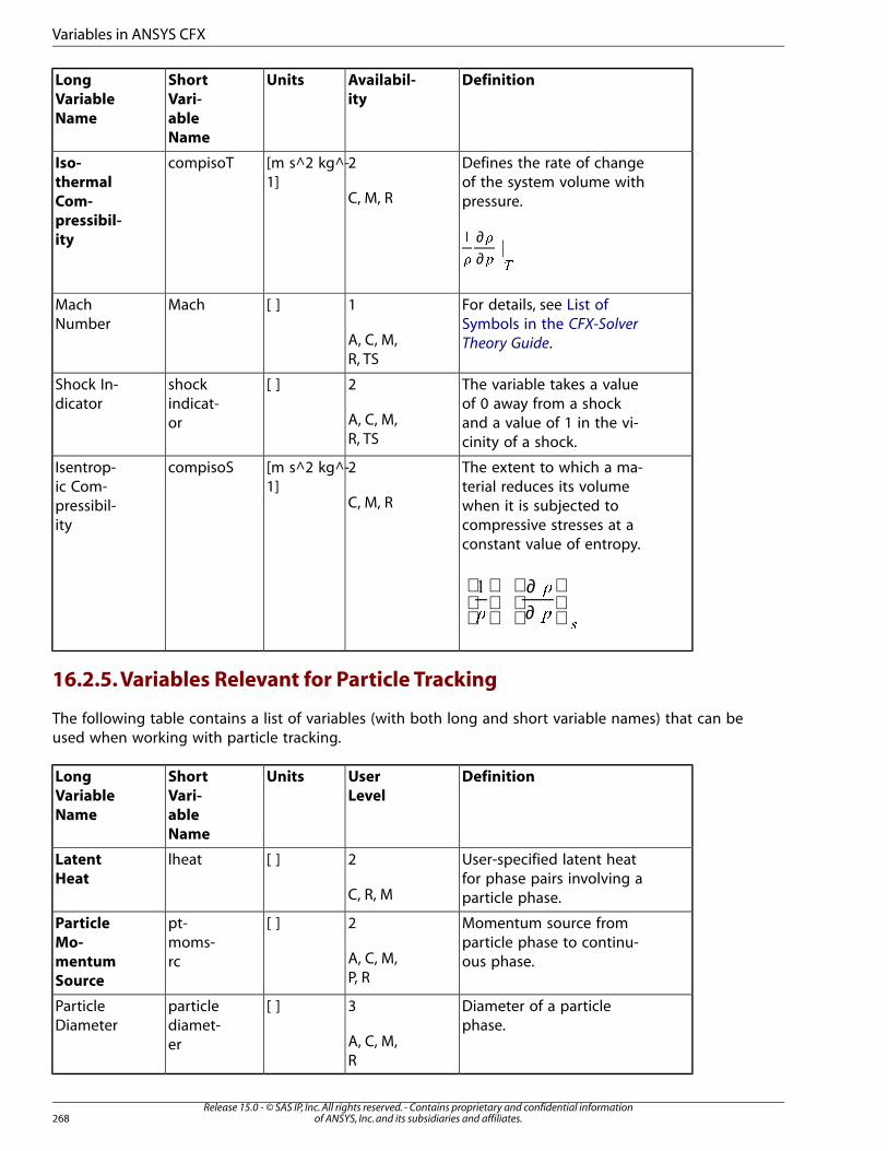
DefinitionAvailabil-
ity
UnitsShort
Vari-
able
Name
Long
Variable
Name
Defines the rate of changeof the system volume withpressure.
2
C, M, R
[m s^2 kg^-1]
compisoTIso-
thermal
Com-
∂∂�
�
��
�
pressibil-
ity
For details, see List ofSymbols in the CFX-Solver
Theory Guide.
1
A, C, M,R, TS
[ ]MachMachNumber
The variable takes a valueof 0 away from a shock
2
A, C, M,R, TS
[ ]shockindicat-or
Shock In-dicator
and a value of 1 in the vi-cinity of a shock.
The extent to which a ma-terial reduces its volume
2
C, M, R
[m s^2 kg^-1]
compisoSIsentrop-ic Com-pressibil-ity
when it is subjected tocompressive stresses at aconstant value of entropy.
∂∂
�
�
��
16.2.5. Variables Relevant for Particle Tracking
The following table contains a list of variables (with both long and short variable names) that can beused when working with particle tracking.
DefinitionUser
Level
UnitsShort
Vari-
able
Name
Long
Variable
Name
User-specified latent heatfor phase pairs involving aparticle phase.
2
C, R, M
[ ]lheatLatent
Heat
Momentum source fromparticle phase to continu-ous phase.
2
A, C, M,P, R
[ ]pt-moms-rc
Particle
Mo-
mentum
Source
Diameter of a particlephase.
3
A, C, M,R
[ ]particlediamet-er
ParticleDiameter
Release 15.0 - © SAS IP, Inc. All rights reserved. - Contains proprietary and confidential informationof ANSYS, Inc. and its subsidiaries and affiliates.268
Variables in ANSYS CFX
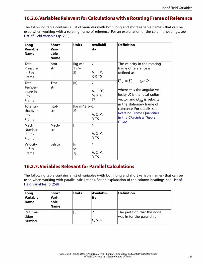
16.2.6.Variables Relevant for Calculations with a Rotating Frame of Reference
The following table contains a list of variables (with both long and short variable names) that can beused when working with a rotating frame of reference. For an explanation of the column headings, seeList of Field Variables (p. 259).
DefinitionAvailabil-
ity
UnitsShort
Vari-
able
Name
Long
Variable
Name
The velocity in the rotatingframe of reference isdefined as:
2
A, C, M,P, R, TS
[kg m^-1 s^-2]
ptot-stn
TotalPressurein StnFrame
= − ×� � � ���� ���2[K]Ttot-stn
TotalTemper-
where is the angular ve-locity, is the local radius
A, C, DT,M, P, R,TS
ature inStnFrame vector, and �� � is velocity
in the stationary frame of2[kg m^2 s^-
2]htot-stn
Total En-thalpy in
reference. For details, seeRotating Frame QuantitiesA, C, M,
R, TSStnFrame
in the CFX-Solver Theory
Guide.1[ ]Mach-
stnMachNumber
A, C, M,R, TS
in StnFrame
1[ms^-1]
velstnVelocityin StnFrame A, C, M,
R, TS
16.2.7. Variables Relevant for Parallel Calculations
The following table contains a list of variables (with both long and short variable names) that can beused when working with parallel calculations. For an explanation of the column headings, see List ofField Variables (p. 259).
DefinitionAvailabil-
ity
UnitsShort
Vari-
able
Name
Long
Variable
Name
The partition that the nodewas in for the parallel run.
2
C, M, R
[ ]Real Par-titionNumber
269Release 15.0 - © SAS IP, Inc. All rights reserved. - Contains proprietary and confidential information
of ANSYS, Inc. and its subsidiaries and affiliates.
List of Field Variables
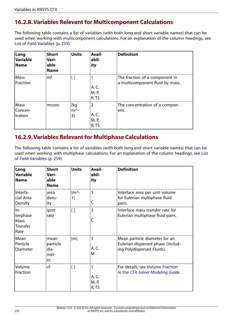
16.2.8. Variables Relevant for Multicomponent Calculations
The following table contains a list of variables (with both long and short variable names) that can beused when working with multicomponent calculations. For an explanation of the column headings, seeList of Field Variables (p. 259).
DefinitionAvail-
abil-
ity
UnitsShort
Vari-
able
Name
Long
Variable
Name
The fraction of a component ina multicomponent fluid by mass.
1
A, C,M, P,R, TS
[ ]mfMassFraction
The concentration of a compon-ent.
2
A, C,M, P,R, TS
[kgm^-3]
mconcMassConcen-tration
16.2.9. Variables Relevant for Multiphase Calculations
The following table contains a list of variables (with both long and short variable names) that can beused when working with multiphase calculations. For an explanation of the column headings, see Listof Field Variables (p. 259).
DefinitionAvail-
abil-
ity
UnitsShort
Vari-
able
Name
Long
Variable
Name
Interface area per unit volumefor Eulerian multiphase fluidpairs.
3
C
[m^-1]
areadens-ity
Interfa-cial AreaDensity
Interface mass transfer rate forEulerian multiphase fluid pairs.
3
C
[ ]ipmtrate
In-terphaseMassTransferRate
Mean particle diameter for anEulerian dispersed phase (includ-ing Polydispersed Fluids).
3
A, C,M
[m]meanparticledia-met-er
MeanParticleDiameter
For details, see Volume Fractionin the CFX-Solver Modeling Guide.
1
A, C,M, P,R, TS
[ ]vfVolumeFraction
Release 15.0 - © SAS IP, Inc. All rights reserved. - Contains proprietary and confidential informationof ANSYS, Inc. and its subsidiaries and affiliates.270
Variables in ANSYS CFX
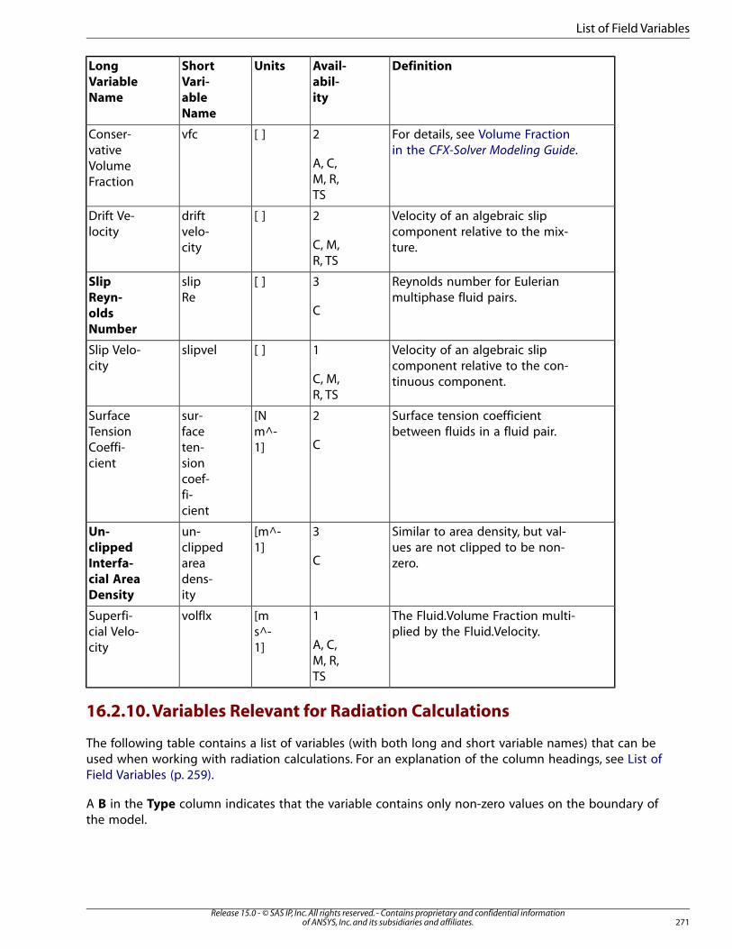
DefinitionAvail-
abil-
ity
UnitsShort
Vari-
able
Name
Long
Variable
Name
For details, see Volume Fractionin the CFX-Solver Modeling Guide.
2
A, C,M, R,TS
[ ]vfcConser-vativeVolumeFraction
Velocity of an algebraic slipcomponent relative to the mix-ture.
2
C, M,R, TS
[ ]driftvelo-city
Drift Ve-locity
Reynolds number for Eulerianmultiphase fluid pairs.
3
C
[ ]slipRe
Slip
Reyn-
olds
Number
Velocity of an algebraic slipcomponent relative to the con-tinuous component.
1
C, M,R, TS
[ ]slipvelSlip Velo-city
Surface tension coefficientbetween fluids in a fluid pair.
2
C
[Nm^-1]
sur-faceten-
SurfaceTensionCoeffi-cient sion
coef-fi-cient
Similar to area density, but val-ues are not clipped to be non-zero.
3
C
[m^-1]
un-clippedarea
Un-
clipped
Interfa-
dens-ity
cial Area
Density
The Fluid.Volume Fraction multi-plied by the Fluid.Velocity.
1
A, C,M, R,TS
[ms^-1]
volflxSuperfi-cial Velo-city
16.2.10. Variables Relevant for Radiation Calculations
The following table contains a list of variables (with both long and short variable names) that can beused when working with radiation calculations. For an explanation of the column headings, see List ofField Variables (p. 259).
A B in the Type column indicates that the variable contains only non-zero values on the boundary ofthe model.
271Release 15.0 - © SAS IP, Inc. All rights reserved. - Contains proprietary and confidential information
of ANSYS, Inc. and its subsidiaries and affiliates.
List of Field Variables
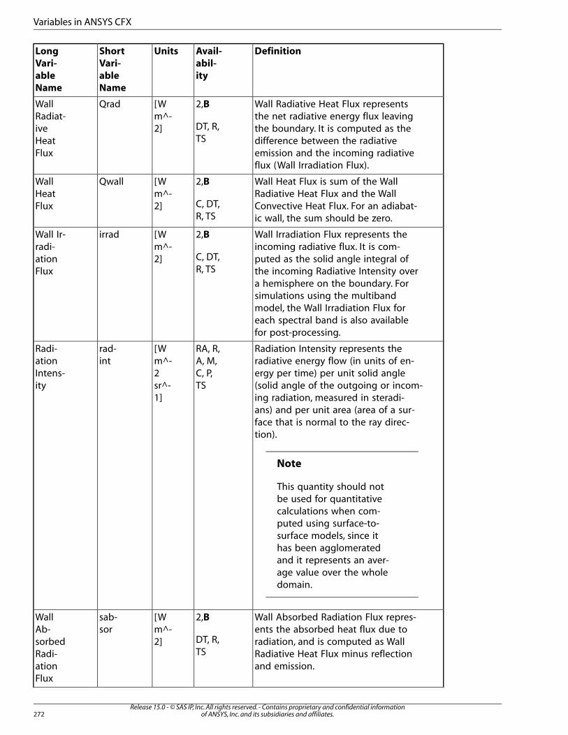
DefinitionAvail-
abil-
ity
UnitsShort
Vari-
able
Name
Long
Vari-
able
Name
Wall Radiative Heat Flux representsthe net radiative energy flux leaving
2,B
DT, R,TS
[Wm^-2]
QradWallRadiat-iveHeatFlux
the boundary. It is computed as thedifference between the radiativeemission and the incoming radiativeflux (Wall Irradiation Flux).
Wall Heat Flux is sum of the WallRadiative Heat Flux and the Wall
2,B
C, DT,R, TS
[Wm^-2]
QwallWallHeatFlux Convective Heat Flux. For an adiabat-
ic wall, the sum should be zero.
Wall Irradiation Flux represents theincoming radiative flux. It is com-
2,B
C, DT,R, TS
[Wm^-2]
irradWall Ir-radi-ationFlux
puted as the solid angle integral ofthe incoming Radiative Intensity overa hemisphere on the boundary. Forsimulations using the multibandmodel, the Wall Irradiation Flux foreach spectral band is also availablefor post-processing.
Radiation Intensity represents theradiative energy flow (in units of en-
RA, R,A, M,
[Wm^-
rad-int
Radi-ation
ergy per time) per unit solid angleC, P,TS
2sr^-1]
Intens-ity (solid angle of the outgoing or incom-
ing radiation, measured in steradi-ans) and per unit area (area of a sur-face that is normal to the ray direc-tion).
Note
This quantity should notbe used for quantitativecalculations when com-puted using surface-to-surface models, since ithas been agglomeratedand it represents an aver-age value over the wholedomain.
Wall Absorbed Radiation Flux repres-ents the absorbed heat flux due to
2,B
DT, R,TS
[Wm^-2]
sab-sor
WallAb-sorbedRadi-
radiation, and is computed as WallRadiative Heat Flux minus reflectionand emission.ation
Flux
Release 15.0 - © SAS IP, Inc. All rights reserved. - Contains proprietary and confidential informationof ANSYS, Inc. and its subsidiaries and affiliates.272
Variables in ANSYS CFX
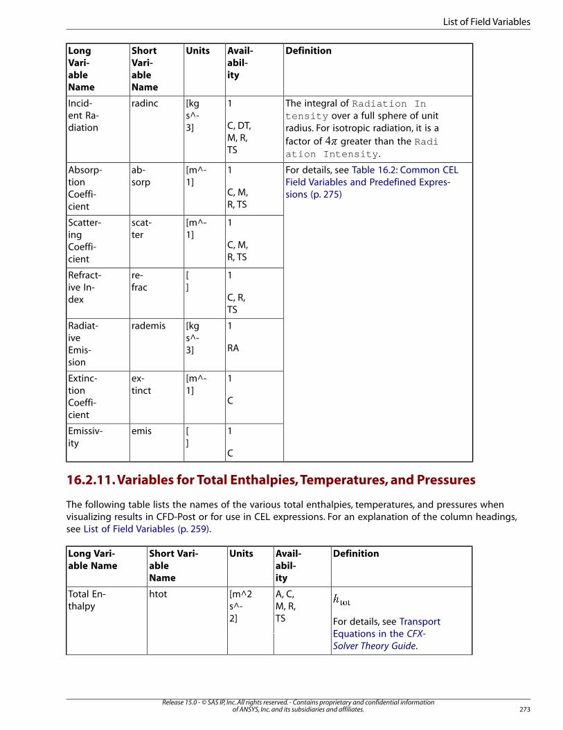
DefinitionAvail-
abil-
ity
UnitsShort
Vari-
able
Name
Long
Vari-
able
Name
The integral of Radiation Intensity over a full sphere of unit
1
C, DT,M, R,TS
[kgs^-3]
radincIncid-ent Ra-diation radius. For isotropic radiation, it is a
factor of � greater than the Radiation Intensity .
For details, see Table 16.2: Common CELField Variables and Predefined Expres-sions (p. 275)
1
C, M,R, TS
[m^-1]
ab-sorp
Absorp-tionCoeffi-cient
1[m^-1]
scat-ter
Scatter-ing
C, M,R, TS
Coeffi-cient
1[]
re-frac
Refract-ive In-dex C, R,
TS
1[kgs^-3]
rademisRadiat-iveEmis-sion
RA
1[m^-1]
ex-tinct
Extinc-tion
CCoeffi-cient
1[]
emisEmissiv-ity
C
16.2.11. Variables for Total Enthalpies, Temperatures, and Pressures
The following table lists the names of the various total enthalpies, temperatures, and pressures whenvisualizing results in CFD-Post or for use in CEL expressions. For an explanation of the column headings,see List of Field Variables (p. 259).
DefinitionAvail-
abil-
ity
UnitsShort Vari-
able
Name
Long Vari-
able Name
����
For details, see TransportEquations in the CFX-
Solver Theory Guide.
A, C,M, R,TS
[m^2s^-2]
htotTotal En-thalpy
273Release 15.0 - © SAS IP, Inc. All rights reserved. - Contains proprietary and confidential information
of ANSYS, Inc. and its subsidiaries and affiliates.
List of Field Variables
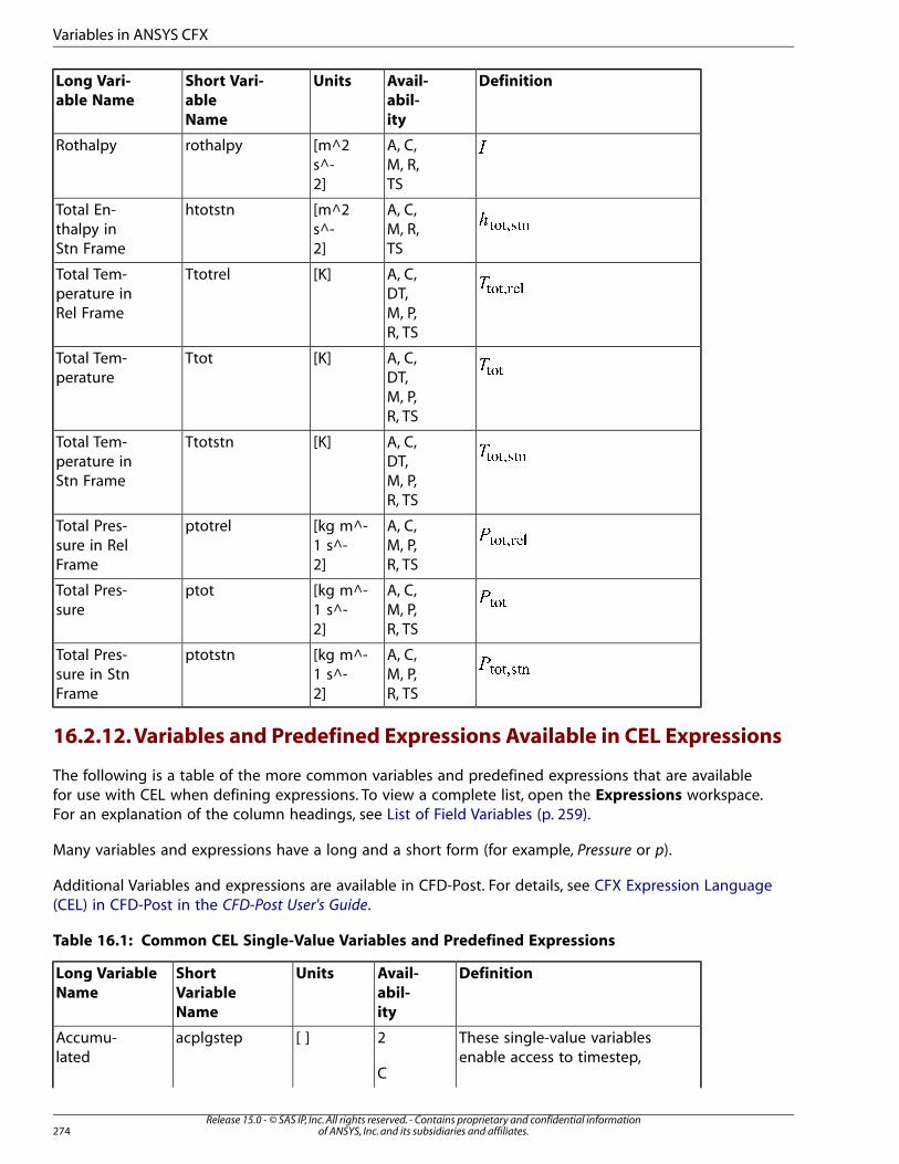
DefinitionAvail-
abil-
ity
UnitsShort Vari-
able
Name
Long Vari-
able Name
�A, C,M, R,TS
[m^2s^-2]
rothalpyRothalpy
��������A, C,M, R,TS
[m^2s^-2]
htotstnTotal En-thalpy inStn Frame
����� A, C,DT,
[K]TtotrelTotal Tem-perature inRel Frame M, P,
R, TS
����A, C,DT,
[K]TtotTotal Tem-perature
M, P,R, TS
��������A, C,DT,
[K]TtotstnTotal Tem-perature inStn Frame M, P,
R, TS
��������A, C,M, P,R, TS
[kg m^-1 s^-2]
ptotrelTotal Pres-sure in RelFrame
�� �A, C,M, P,R, TS
[kg m^-1 s^-2]
ptotTotal Pres-sure
!"#"$%"&A, C,M, P,R, TS
[kg m^-1 s^-2]
ptotstnTotal Pres-sure in StnFrame
16.2.12. Variables and Predefined Expressions Available in CEL Expressions
The following is a table of the more common variables and predefined expressions that are availablefor use with CEL when defining expressions. To view a complete list, open the Expressions workspace.For an explanation of the column headings, see List of Field Variables (p. 259).
Many variables and expressions have a long and a short form (for example, Pressure or p).
Additional Variables and expressions are available in CFD-Post. For details, see CFX Expression Language(CEL) in CFD-Post in the CFD-Post User's Guide.
Table 16.1: Common CEL Single-Value Variables and Predefined Expressions
DefinitionAvail-
abil-
ity
UnitsShort
Variable
Name
Long Variable
Name
These single-value variablesenable access to timestep,
2
C
[ ]acplgstepAccumu-lated
Release 15.0 - © SAS IP, Inc. All rights reserved. - Contains proprietary and confidential informationof ANSYS, Inc. and its subsidiaries and affiliates.274
Variables in ANSYS CFX
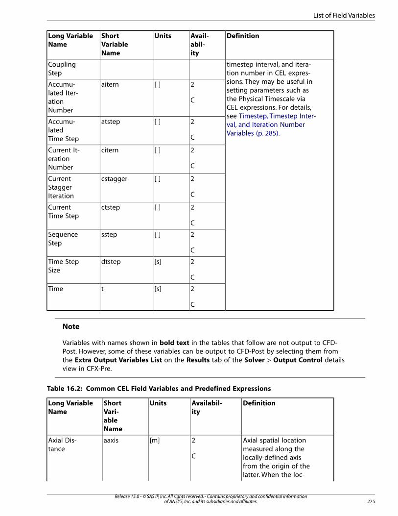
DefinitionAvail-
abil-
ity
UnitsShort
Variable
Name
Long Variable
Name
CouplingStep
timestep interval, and itera-tion number in CEL expres-sions. They may be useful in2[ ]aiternAccumu-
lated Iter- setting parameters such asthe Physical Timescale viaCation
Number CEL expressions. For details,see Timestep, Timestep Inter-
2[ ]atstepAccumu-latedTime Step
val, and Iteration NumberVariables (p. 285).
C
2[ ]citernCurrent It-erationNumber C
2[ ]cstaggerCurrentStaggerIteration C
2[ ]ctstepCurrentTime Step
C
2[ ]sstepSequenceStep
C
2[s]dtstepTime StepSize
C
2[s]tTime
C
Note
Variables with names shown in bold text in the tables that follow are not output to CFD-Post. However, some of these variables can be output to CFD-Post by selecting them fromthe Extra Output Variables List on the Results tab of the Solver > Output Control detailsview in CFX-Pre.
Table 16.2: Common CEL Field Variables and Predefined Expressions
DefinitionAvailabil-
ity
UnitsShort
Vari-
able
Name
Long Variable
Name
Axial spatial locationmeasured along the
2
C
[m]aaxisAxial Dis-tance
locally-defined axisfrom the origin of thelatter. When the loc-
275Release 15.0 - © SAS IP, Inc. All rights reserved. - Contains proprietary and confidential information
of ANSYS, Inc. and its subsidiaries and affiliates.
List of Field Variables
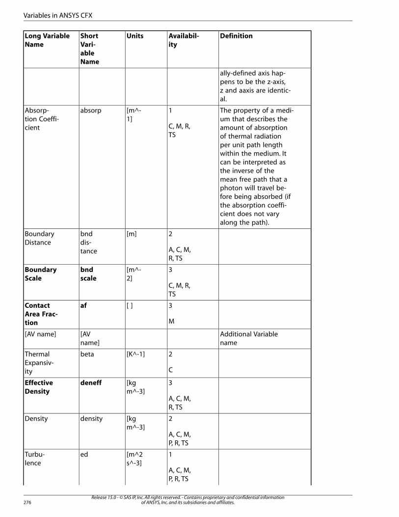
DefinitionAvailabil-
ity
UnitsShort
Vari-
able
Name
Long Variable
Name
ally-defined axis hap-pens to be the z-axis,z and aaxis are identic-al.
The property of a medi-um that describes the
1
C, M, R,TS
[m^-1]
absorpAbsorp-tion Coeffi-cient amount of absorption
of thermal radiationper unit path lengthwithin the medium. Itcan be interpreted asthe inverse of themean free path that aphoton will travel be-fore being absorbed (ifthe absorption coeffi-cient does not varyalong the path).
2[m]bnddis-tance
BoundaryDistance
A, C, M,R, TS
3[m^-2]
bnd
scale
Boundary
ScaleC, M, R,TS
3[ ]afContact
Area Frac-
tion M
Additional Variablename
[AVname]
[AV name]
2[K^-1]betaThermalExpansiv-ity C
3[kgm^-3]
deneffEffective
DensityA, C, M,R, TS
2[kgm^-3]
densityDensity
A, C, M,P, R, TS
1[m^2s^-3]
edTurbu-lence
A, C, M,P, R, TS
Release 15.0 - © SAS IP, Inc. All rights reserved. - Contains proprietary and confidential informationof ANSYS, Inc. and its subsidiaries and affiliates.276
Variables in ANSYS CFX
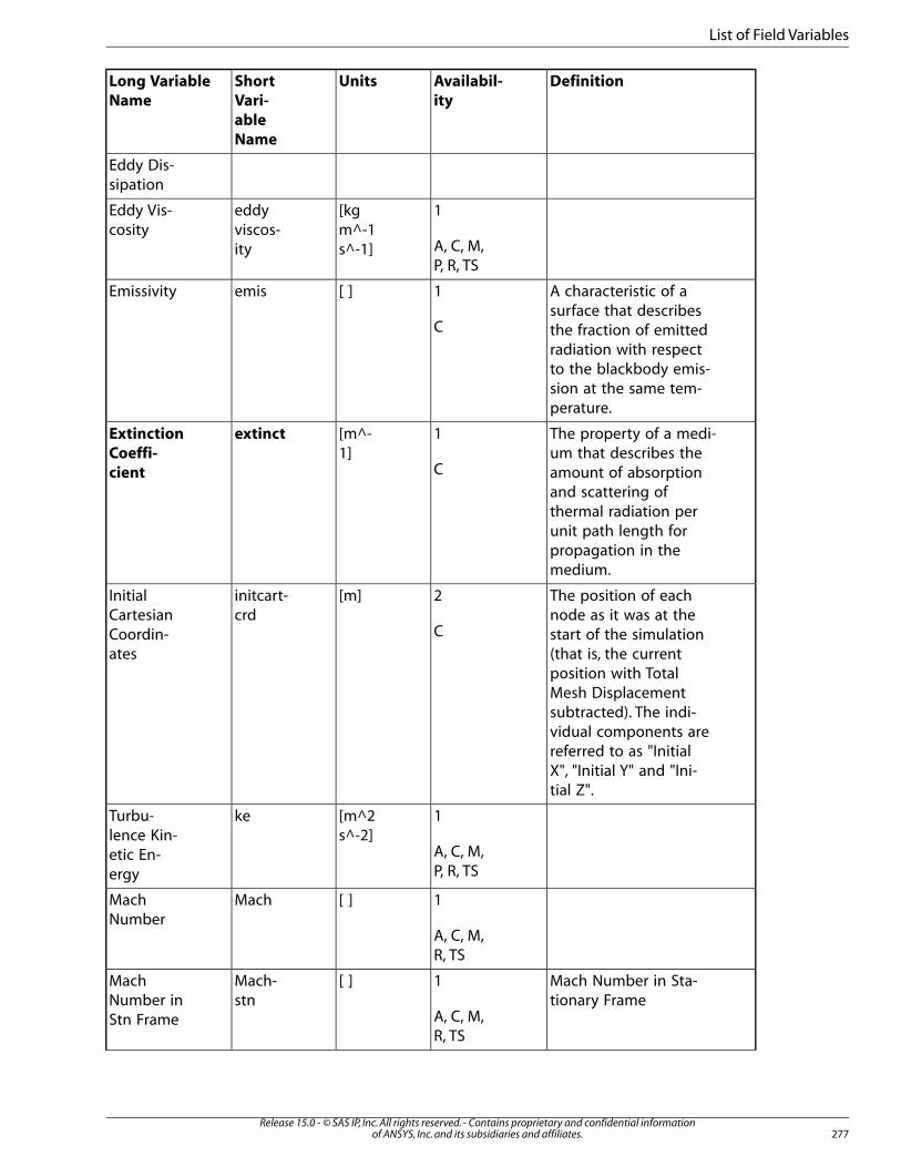
DefinitionAvailabil-
ity
UnitsShort
Vari-
able
Name
Long Variable
Name
Eddy Dis-sipation
1[kgm^-1s^-1]
eddyviscos-ity
Eddy Vis-cosity
A, C, M,P, R, TS
A characteristic of asurface that describes
1
C
[ ]emisEmissivity
the fraction of emittedradiation with respectto the blackbody emis-sion at the same tem-perature.
The property of a medi-um that describes the
1
C
[m^-1]
extinctExtinction
Coeffi-
cient amount of absorptionand scattering ofthermal radiation perunit path length forpropagation in themedium.
The position of eachnode as it was at the
2
C
[m]initcart-crd
InitialCartesianCoordin-ates
start of the simulation(that is, the currentposition with TotalMesh Displacementsubtracted). The indi-vidual components arereferred to as "InitialX", "Initial Y" and "Ini-tial Z".
1[m^2s^-2]
keTurbu-lence Kin-
A, C, M,P, R, TS
etic En-ergy
1[ ]MachMachNumber
A, C, M,R, TS
Mach Number in Sta-tionary Frame
1
A, C, M,R, TS
[ ]Mach-stn
MachNumber inStn Frame
277Release 15.0 - © SAS IP, Inc. All rights reserved. - Contains proprietary and confidential information
of ANSYS, Inc. and its subsidiaries and affiliates.
List of Field Variables
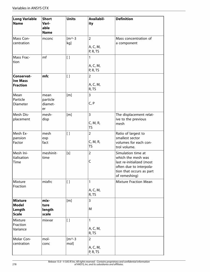
DefinitionAvailabil-
ity
UnitsShort
Vari-
able
Name
Long Variable
Name
Mass concentration ofa component
2
A, C, M,P, R, TS
[m^-3kg]
mconcMass Con-centration
1[ ]mfMass Frac-tion
A, C, M,P, R, TS
2[ ]mfcConservat-
ive Mass
Fraction A, C, M,R, TS
3[m]meanparticle
MeanParticleDiameter C, Pdiamet-
er
The displacement relat-ive to the previousmesh
3
C, M, R,TS
[m]mesh-disp
Mesh Dis-placement
Ratio of largest tosmallest sector
2
C, M, R,TS
[ ]meshexpfact
Mesh Ex-pansionFactor volumes for each con-
trol volume.
Simulation time atwhich the mesh was
2
C
[s]meshinit-time
Mesh Ini-tialisationTime last re-initialized (most
often due to interpola-tion that occurs as partof remeshing)
Mixture Fraction Mean1[ ]mixfrcMixtureFraction
A, C, M,R, TS
3[m]mix-
ture
Mixture
ModelMlength
scale
Length
Scale
1[ ]mixvarMixtureFractionVariance A, C, M,
R, TS
2[m^-3mol]
mol-conc
Molar Con-centration
A, C, M,P, R, TS
Release 15.0 - © SAS IP, Inc. All rights reserved. - Contains proprietary and confidential informationof ANSYS, Inc. and its subsidiaries and affiliates.278
Variables in ANSYS CFX
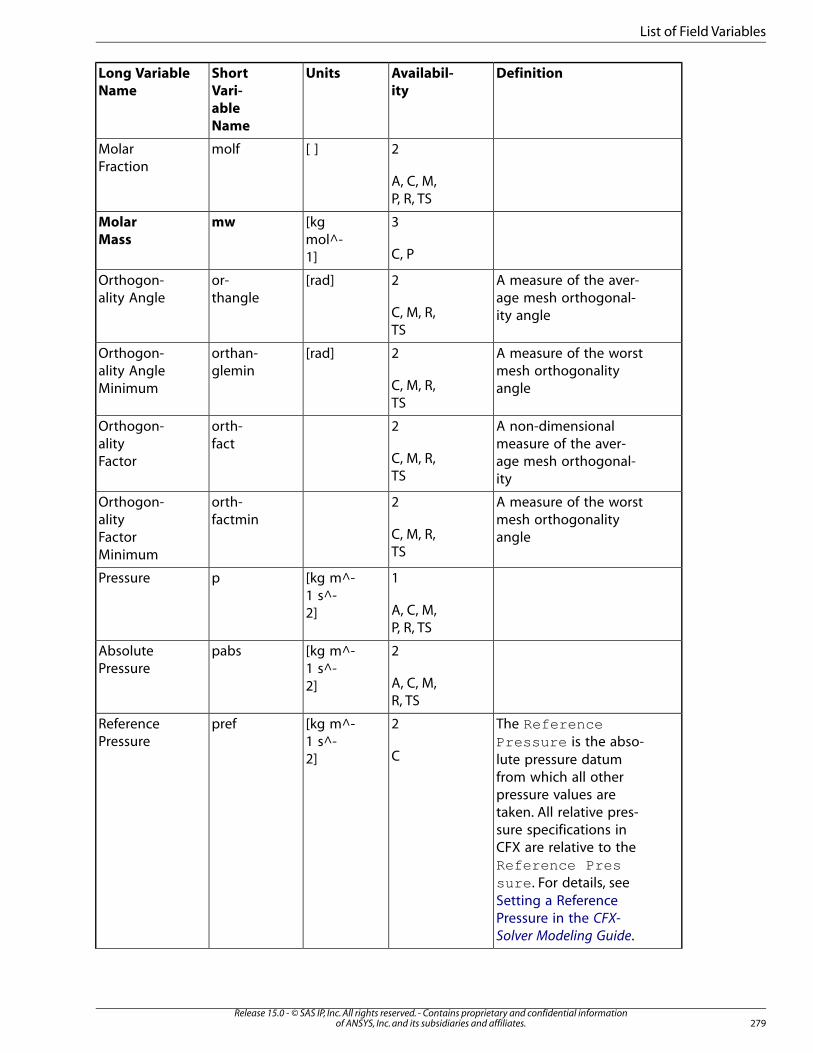
DefinitionAvailabil-
ity
UnitsShort
Vari-
able
Name
Long Variable
Name
2[ ]molfMolarFraction
A, C, M,P, R, TS
3[kgmol^-1]
mwMolar
MassC, P
A measure of the aver-age mesh orthogonal-ity angle
2
C, M, R,TS
[rad]or-thangle
Orthogon-ality Angle
A measure of the worstmesh orthogonalityangle
2
C, M, R,TS
[rad]orthan-glemin
Orthogon-ality AngleMinimum
A non-dimensionalmeasure of the aver-
2
C, M, R,TS
orth-fact
Orthogon-alityFactor age mesh orthogonal-
ity
A measure of the worstmesh orthogonalityangle
2
C, M, R,TS
orth-factmin
Orthogon-alityFactorMinimum
1[kg m^-1 s^-2]
pPressure
A, C, M,P, R, TS
2[kg m^-1 s^-2]
pabsAbsolutePressure
A, C, M,R, TS
The ReferencePressure is the abso-
2
C
[kg m^-1 s^-2]
prefReferencePressure
lute pressure datumfrom which all otherpressure values aretaken. All relative pres-sure specifications inCFX are relative to theReference Pressure . For details, seeSetting a ReferencePressure in the CFX-
Solver Modeling Guide.
279Release 15.0 - © SAS IP, Inc. All rights reserved. - Contains proprietary and confidential information
of ANSYS, Inc. and its subsidiaries and affiliates.
List of Field Variables
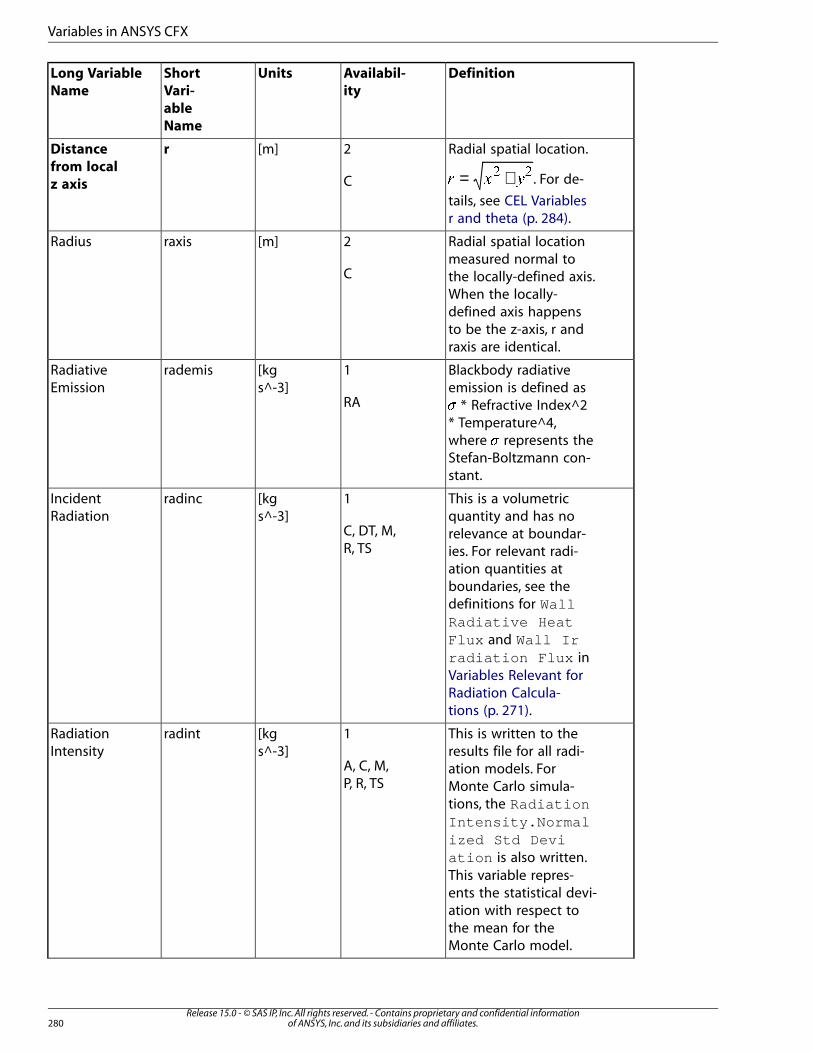
DefinitionAvailabil-
ity
UnitsShort
Vari-
able
Name
Long Variable
Name
Radial spatial location.
= +� � �� �
. For de-
2
C
[m]rDistance
from local
z axistails, see CEL Variablesr and theta (p. 284).
Radial spatial locationmeasured normal to
2
C
[m]raxisRadius
the locally-defined axis.When the locally-defined axis happensto be the z-axis, r andraxis are identical.
Blackbody radiativeemission is defined as
1
RA
[kgs^-3]
rademisRadiativeEmission
� * Refractive Index^2* Temperature^4,where � represents theStefan-Boltzmann con-stant.
This is a volumetricquantity and has no
1
C, DT, M,R, TS
[kgs^-3]
radincIncidentRadiation
relevance at boundar-ies. For relevant radi-ation quantities atboundaries, see thedefinitions for WallRadiative HeatFlux and Wall Irradiation Flux inVariables Relevant forRadiation Calcula-tions (p. 271).
This is written to theresults file for all radi-
1
A, C, M,P, R, TS
[kgs^-3]
radintRadiationIntensity
ation models. ForMonte Carlo simula-tions, the RadiationIntensity.Normalized Std Deviation is also written.This variable repres-ents the statistical devi-ation with respect tothe mean for theMonte Carlo model.
Release 15.0 - © SAS IP, Inc. All rights reserved. - Contains proprietary and confidential informationof ANSYS, Inc. and its subsidiaries and affiliates.280
Variables in ANSYS CFX
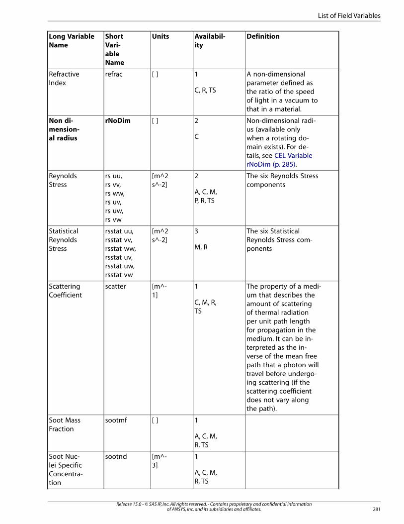
DefinitionAvailabil-
ity
UnitsShort
Vari-
able
Name
Long Variable
Name
A non-dimensionalparameter defined as
1
C, R, TS
[ ]refracRefractiveIndex
the ratio of the speedof light in a vacuum tothat in a material.
Non-dimensional radi-us (available only
2
C
[ ]rNoDimNon di-
mension-
al radius when a rotating do-main exists). For de-tails, see CEL VariablerNoDim (p. 285).
The six Reynolds Stresscomponents
2
A, C, M,P, R, TS
[m^2s^-2]
rs uu,rs vv,rs ww,rs uv,
ReynoldsStress
rs uw,rs vw
The six StatisticalReynolds Stress com-ponents
3
M, R
[m^2s^-2]
rsstat uu,rsstat vv,rsstat ww,
StatisticalReynoldsStress
rsstat uv,rsstat uw,rsstat vw
The property of a medi-um that describes the
1
C, M, R,TS
[m^-1]
scatterScatteringCoefficient
amount of scatteringof thermal radiationper unit path lengthfor propagation in themedium. It can be in-terpreted as the in-verse of the mean freepath that a photon willtravel before undergo-ing scattering (if thescattering coefficientdoes not vary alongthe path).
1[ ]sootmfSoot MassFraction
A, C, M,R, TS
1[m^-3]
sootnclSoot Nuc-lei Specific
A, C, M,R, TS
Concentra-tion
281Release 15.0 - © SAS IP, Inc. All rights reserved. - Contains proprietary and confidential information
of ANSYS, Inc. and its subsidiaries and affiliates.
List of Field Variables
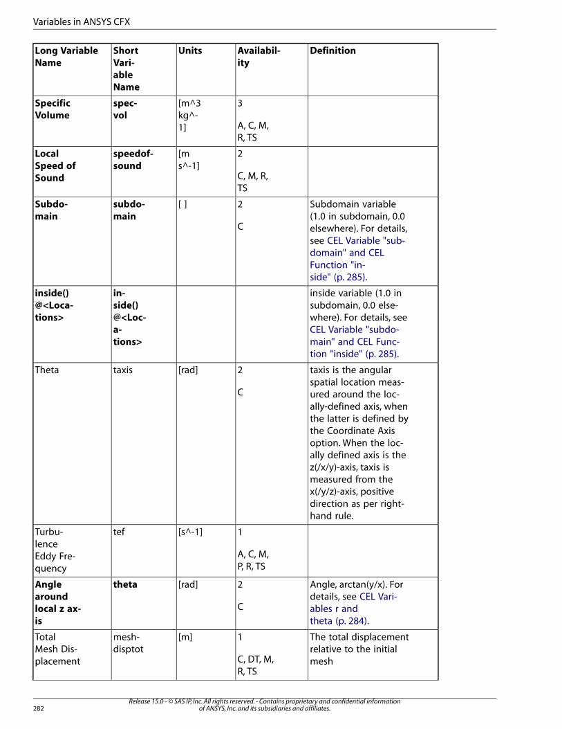
DefinitionAvailabil-
ity
UnitsShort
Vari-
able
Name
Long Variable
Name
3[m^3kg^-1]
spec-
vol
Specific
VolumeA, C, M,R, TS
2[ms^-1]
speedof-
sound
Local
Speed of
Sound C, M, R,TS
Subdomain variable(1.0 in subdomain, 0.0
2
C
[ ]subdo-
main
Subdo-
main
elsewhere). For details,see CEL Variable "sub-domain" and CELFunction "in-side" (p. 285).
inside variable (1.0 insubdomain, 0.0 else-
in-
side()
inside()
@<Loca-
tions> where). For details, see@<Loc-
CEL Variable "subdo-a-
tions> main" and CEL Func-tion "inside" (p. 285).
taxis is the angularspatial location meas-
2
C
[rad]taxisTheta
ured around the loc-ally-defined axis, whenthe latter is defined bythe Coordinate Axisoption. When the loc-ally defined axis is thez(/x/y)-axis, taxis ismeasured from thex(/y/z)-axis, positivedirection as per right-hand rule.
1[s^-1]tefTurbu-lence
A, C, M,P, R, TS
Eddy Fre-quency
Angle, arctan(y/x). Fordetails, see CEL Vari-
2
C
[rad]thetaAngle
around
local z ax-
is
ables r andtheta (p. 284).
The total displacementrelative to the initialmesh
1
C, DT, M,R, TS
[m]mesh-disptot
TotalMesh Dis-placement
Release 15.0 - © SAS IP, Inc. All rights reserved. - Contains proprietary and confidential informationof ANSYS, Inc. and its subsidiaries and affiliates.282
Variables in ANSYS CFX
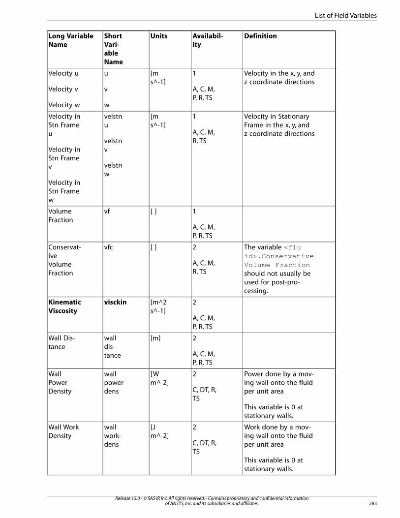
DefinitionAvailabil-
ity
UnitsShort
Vari-
able
Name
Long Variable
Name
Velocity in the x, y, andz coordinate directions
1
A, C, M,P, R, TS
[ms^-1]
u
v
w
Velocity u
Velocity v
Velocity w
Velocity in StationaryFrame in the x, y, andz coordinate directions
1
A, C, M,R, TS
[ms^-1]
velstnu
velstnv
Velocity inStn Frameu
Velocity inStn Framev velstn
wVelocity inStn Framew
1[ ]vfVolumeFraction
A, C, M,P, R, TS
The variable <fluid>.Conservative
2
A, C, M,R, TS
[ ]vfcConservat-iveVolumeFraction
Volume Fractionshould not usually beused for post-pro-cessing.
2[m^2s^-1]
visckinKinematic
ViscosityA, C, M,P, R, TS
2[m]walldis-tance
Wall Dis-tance
A, C, M,P, R, TS
Power done by a mov-ing wall onto the fluidper unit area
2
C, DT, R,TS
[Wm^-2]
wallpower-dens
WallPowerDensity
This variable is 0 atstationary walls.
Work done by a mov-ing wall onto the fluidper unit area
2
C, DT, R,TS
[Jm^-2]
wallwork-dens
Wall WorkDensity
This variable is 0 atstationary walls.
283Release 15.0 - © SAS IP, Inc. All rights reserved. - Contains proprietary and confidential information
of ANSYS, Inc. and its subsidiaries and affiliates.
List of Field Variables
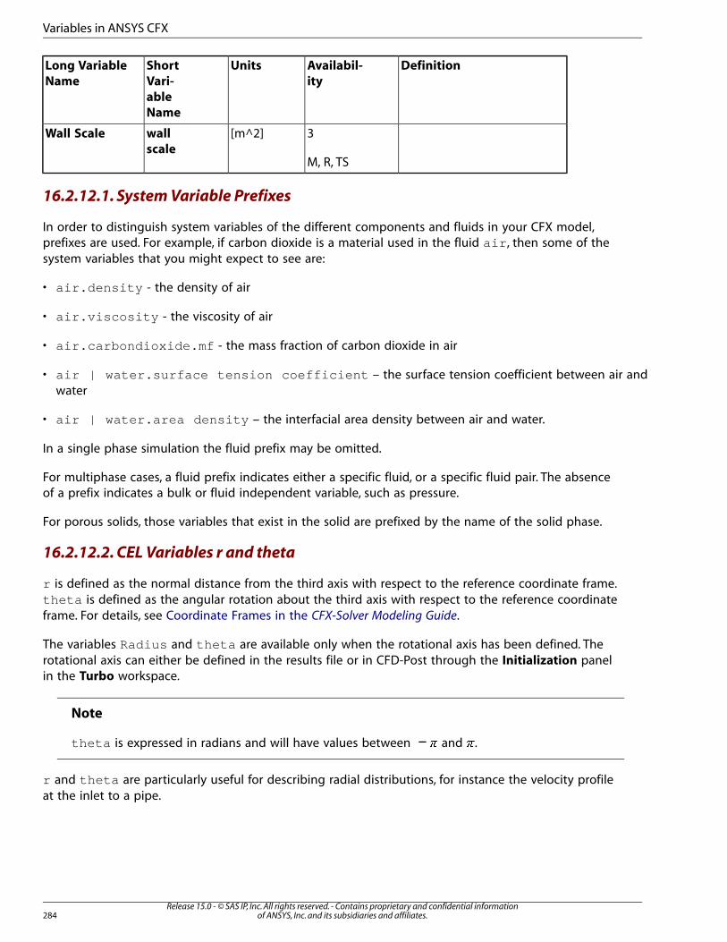
DefinitionAvailabil-
ity
UnitsShort
Vari-
able
Name
Long Variable
Name
3[m^2]wall
scale
Wall Scale
M, R, TS
16.2.12.1. System Variable Prefixes
In order to distinguish system variables of the different components and fluids in your CFX model,prefixes are used. For example, if carbon dioxide is a material used in the fluid air , then some of thesystem variables that you might expect to see are:
• air.density - the density of air
• air.viscosity - the viscosity of air
• air.carbondioxide.mf - the mass fraction of carbon dioxide in air
• air | water.surface tension coefficient – the surface tension coefficient between air andwater
• air | water.area density – the interfacial area density between air and water.
In a single phase simulation the fluid prefix may be omitted.
For multiphase cases, a fluid prefix indicates either a specific fluid, or a specific fluid pair. The absenceof a prefix indicates a bulk or fluid independent variable, such as pressure.
For porous solids, those variables that exist in the solid are prefixed by the name of the solid phase.
16.2.12.2. CEL Variables r and theta
r is defined as the normal distance from the third axis with respect to the reference coordinate frame.theta is defined as the angular rotation about the third axis with respect to the reference coordinateframe. For details, see Coordinate Frames in the CFX-Solver Modeling Guide.
The variables Radius and theta are available only when the rotational axis has been defined. Therotational axis can either be defined in the results file or in CFD-Post through the Initialization panelin the Turbo workspace.
Note
theta is expressed in radians and will have values between − � and �.
r and theta are particularly useful for describing radial distributions, for instance the velocity profileat the inlet to a pipe.
Release 15.0 - © SAS IP, Inc. All rights reserved. - Contains proprietary and confidential informationof ANSYS, Inc. and its subsidiaries and affiliates.284
Variables in ANSYS CFX
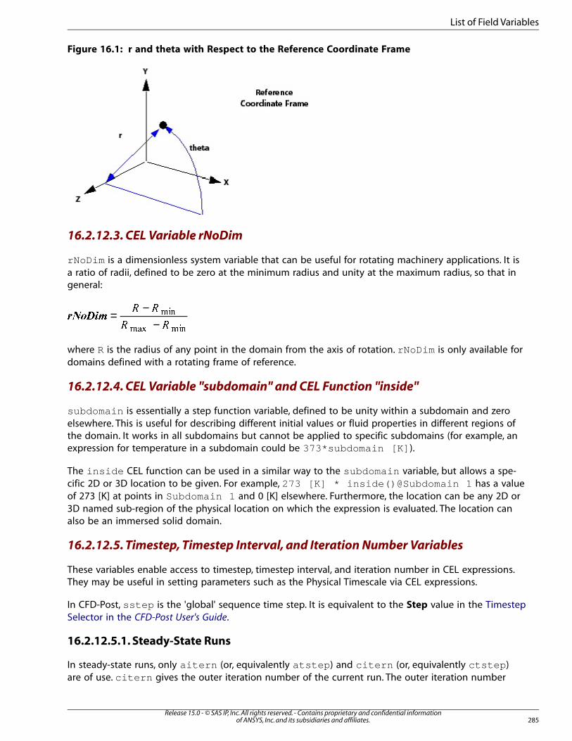
Figure 16.1: r and theta with Respect to the Reference Coordinate Frame
16.2.12.3. CEL Variable rNoDim
rNoDim is a dimensionless system variable that can be useful for rotating machinery applications. It isa ratio of radii, defined to be zero at the minimum radius and unity at the maximum radius, so that ingeneral:
= −−
������� �
� �
��
�� ��
where R is the radius of any point in the domain from the axis of rotation. rNoDim is only available fordomains defined with a rotating frame of reference.
16.2.12.4. CEL Variable "subdomain" and CEL Function "inside"
subdomain is essentially a step function variable, defined to be unity within a subdomain and zeroelsewhere. This is useful for describing different initial values or fluid properties in different regions ofthe domain. It works in all subdomains but cannot be applied to specific subdomains (for example, anexpression for temperature in a subdomain could be 373*subdomain [K] ).
The inside CEL function can be used in a similar way to the subdomain variable, but allows a spe-cific 2D or 3D location to be given. For example, 273 [K] * inside()@Subdomain 1 has a valueof 273 [K] at points in Subdomain 1 and 0 [K] elsewhere. Furthermore, the location can be any 2D or3D named sub-region of the physical location on which the expression is evaluated. The location canalso be an immersed solid domain.
16.2.12.5. Timestep, Timestep Interval, and Iteration Number Variables
These variables enable access to timestep, timestep interval, and iteration number in CEL expressions.They may be useful in setting parameters such as the Physical Timescale via CEL expressions.
In CFD-Post, sstep is the 'global' sequence time step. It is equivalent to the Step value in the TimestepSelector in the CFD-Post User's Guide.
16.2.12.5.1. Steady-State Runs
In steady-state runs, only aitern (or, equivalently atstep ) and citern (or, equivalently ctstep )are of use. citern gives the outer iteration number of the current run. The outer iteration number
285Release 15.0 - © SAS IP, Inc. All rights reserved. - Contains proprietary and confidential information
of ANSYS, Inc. and its subsidiaries and affiliates.
List of Field Variables
begins at 1 for each run, irrespective of whether it is a restarted run. aitern gives the accumulatedouter iteration number, which accumulates across a restarted run.
16.2.12.5.2. Transient Runs
In transient runs, atstep and ctstep are used for the accumulated and current timestep numbersof the outer timestep loop. citern gives the current coefficient loop number within the currenttimestep. Thus, citern will cycle between 1 and n for each timestep during a transient run, where nis the number of coefficient loops. aitern is equivalent to citern for transient runs.
16.2.12.5.3. ANSYS Multi-field Runs
For ANSYS Multi-field runs, cstagger and acplgstep are also available. cstagger gives the currentstagger iteration, which will cycle between 1 and n for each coupling step of the run. acplgstep givesthe accumulated coupling step. This gives the multi-field timestep number or "coupling step" numberfor the run, and accumulates across a restarted run. For transient ANSYS Multi-field runs where the CFXtimestep is the same as the multi-field timestep, acplgstep is equivalent to atstep .
16.2.12.6. Expression Names
Your CEL expression name can be any name that does not conflict with the name of a CFX systemvariable, mathematical function, or an existing CEL expression. The RULES and VARIABLES files provideinformation on valid options, variables, and dependencies. Both files are located in <CFXROOT>/etc/and can be viewed in any text editor.
16.2.12.7. Scalar Expressions
A scalar expression is a real valued expression using predefined variables, user variables, and literalconstants (for example, 1.0). Note that literal constants have to be of the same dimension. Scalar expres-sions can include the operators + - * / and ^ and several of the mathematical functions found instandard Fortran (for example, sin() and exp()).
An expression’s value is a real value and has specified dimensions (except where it is dimensionless -but this is also a valid dimension setting).
For example, if t is time and L is a length then the result of L/t has the same dimensions as speed.
The + and - operators are only valid between expressions with the same dimensions and result in anexpression of those dimensions.
The * and / operators combine the dimensions of their operands in the usual fashion. X^I, where I isan integer, results in an expression whose dimensions are those of X to the power I. The trigonometricfunctions all work in terms of an angle in radians and a dimensionless ratio.
16.2.12.8. Expression Properties
There are three properties of expressions:
• An expression is a simple expression if the only operations are +, -, *, / and there are no functions usedin the expression.
• An expression is a constant expression if all the numbers in the expression are explicit (that is, they donot depend on values from the solver).
Release 15.0 - © SAS IP, Inc. All rights reserved. - Contains proprietary and confidential informationof ANSYS, Inc. and its subsidiaries and affiliates.286
Variables in ANSYS CFX
• An expression is an integer expression if all the numbers in the expression are integers and the result ofeach function or operation is an integer.
For example, (3+5)/2 is a simple, constant, integer expression. However, 2*(1/2) is not a constant integerexpression because the result of 1/2 is 0.5, not an integer. Also 3.*4 is not a constant integer expressionbecause 3 is not an integer. Moreover, 2^3 is not a simple, constant, integer expression because ^ isnot in the list (+, -, *, /).
Expressions are evaluated at runtime and in single precision floating point arithmetic.
16.2.12.9. Available and Unavailable Variables
CFX System Variables and user-defined expressions will be available or unavailable depending on thesimulation you are performing and the expressions you want to create. In some circumstances, SystemVariables are logically unavailable; for instance, time (t ) is not available for steady-state simulations. Inothers, the availability of a System Variable is not allowed for physical model reasons. For example,density can be a function of pressure (p), temperature (T) and location (x , y , z ), but no other systemvariables.
Information on how to find dependencies for all parameters is available in the RULES and VARIABLESfiles. Both files are located in <CFXROOT>/etc/ and can be viewed in any text editor.
The expression definition can depend on any system variable. If, however, that expression depends ona system variable that is unavailable for a particular context, then that expression will also be unavailable.
16.3. Particle Variables Generated by the Solver
This section describes the following types of particle variables that you may have defined in CFX-Preor that are available for viewing in CFD-Post and exporting to other files. Many variables are relevantonly for specific physical models.
16.3.1. Particle Track Variables16.3.2. Particle Field Variables
Some variables are defined only on the boundaries of the model. When using these variables in CFD-Post, there are a limited number of useful things that you can do with these. For details, see Boundary-Value-Only Variables in the CFD-Post User's Guide.
The following information is given for particle variables described in this section:
• Long Variable Name: The name that you see in the user interface.
• Short Variable Name: The name that must be used in CEL expressions.
• Units: The default units for the variable. An empty entry [ ] indicates a dimensionless variable.
Note
The entries in the Units columns are SI but could as easily be any other system of units.
• Type (User Level, Boundary)
User Level: This number is useful when using the CFX Export facility. For details, see File ExportUtility in the CFX-Solver Manager User's Guide. Note that the CFX-Solver may sometimes override the
287Release 15.0 - © SAS IP, Inc. All rights reserved. - Contains proprietary and confidential information
of ANSYS, Inc. and its subsidiaries and affiliates.
Particle Variables Generated by the Solver
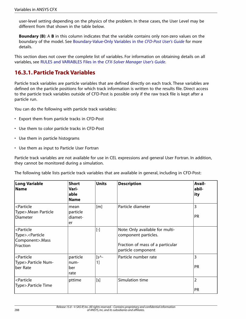
user-level setting depending on the physics of the problem. In these cases, the User Level may bedifferent from that shown in the table below.
Boundary (B): A B in this column indicates that the variable contains only non-zero values on theboundary of the model. See Boundary-Value-Only Variables in the CFD-Post User's Guide for moredetails.
This section does not cover the complete list of variables. For information on obtaining details on allvariables, see RULES and VARIABLES Files in the CFX-Solver Manager User's Guide.
16.3.1. Particle Track Variables
Particle track variables are particle variables that are defined directly on each track. These variables aredefined on the particle positions for which track information is written to the results file. Direct accessto the particle track variables outside of CFD-Post is possible only if the raw track file is kept after aparticle run.
You can do the following with particle track variables:
• Export them from particle tracks in CFD-Post
• Use them to color particle tracks in CFD-Post
• Use them in particle histograms
• Use them as input to Particle User Fortran
Particle track variables are not available for use in CEL expressions and general User Fortran. In addition,they cannot be monitored during a simulation.
The following table lists particle track variables that are available in general, including in CFD-Post:
Avail-
abil-
ity
DescriptionUnitsShort
Vari-
able
Name
Long Variable
Name
3Particle diameter[m]meanparticle
<ParticleType>.Mean ParticleDiameter PRdiamet-
er
Note: Only available for multi-component particles.
[-]<ParticleType>.<Particle
Fraction of mass of a particularparticle component
Component>.MassFraction
3Particle number rate[s^-1]
particlenum-
<ParticleType>.Particle Num-ber Rate PRber
rate
2Simulation time[s]pttime<ParticleType>.Particle Time
PR
Release 15.0 - © SAS IP, Inc. All rights reserved. - Contains proprietary and confidential informationof ANSYS, Inc. and its subsidiaries and affiliates.288
Variables in ANSYS CFX
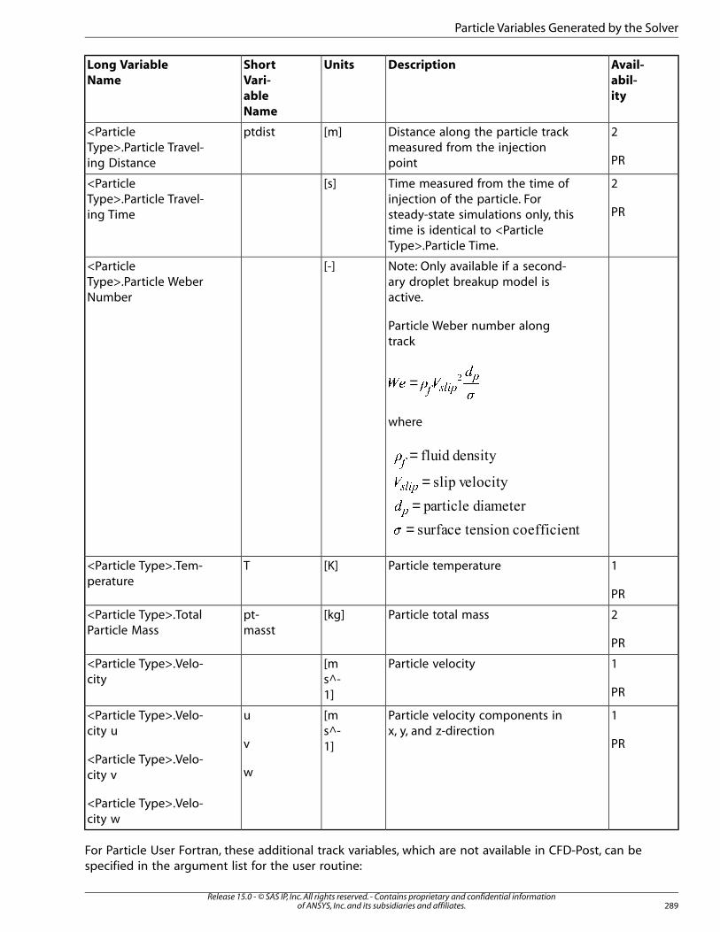
Avail-
abil-
ity
DescriptionUnitsShort
Vari-
able
Name
Long Variable
Name
2Distance along the particle trackmeasured from the injectionpoint
[m]ptdist<ParticleType>.Particle Travel-ing Distance PR
2Time measured from the time ofinjection of the particle. For
[s]<ParticleType>.Particle Travel-ing Time PRsteady-state simulations only, this
time is identical to <ParticleType>.Particle Time.
Note: Only available if a second-ary droplet breakup model isactive.
[-]<ParticleType>.Particle WeberNumber
Particle Weber number alongtrack
=�� � ��
�� ��
�
where
=
==
=
�
�
�
�
����
�
1Particle temperature[K]T<Particle Type>.Tem-perature
PR
2Particle total mass[kg]pt-masst
<Particle Type>.TotalParticle Mass
PR
1Particle velocity[ms^-1]
<Particle Type>.Velo-city
PR
1Particle velocity components inx, y, and z-direction
[ms^-1]
u
v
w
<Particle Type>.Velo-city u
<Particle Type>.Velo-city v
PR
<Particle Type>.Velo-city w
For Particle User Fortran, these additional track variables, which are not available in CFD-Post, can bespecified in the argument list for the user routine:
289Release 15.0 - © SAS IP, Inc. All rights reserved. - Contains proprietary and confidential information
of ANSYS, Inc. and its subsidiaries and affiliates.
Particle Variables Generated by the Solver
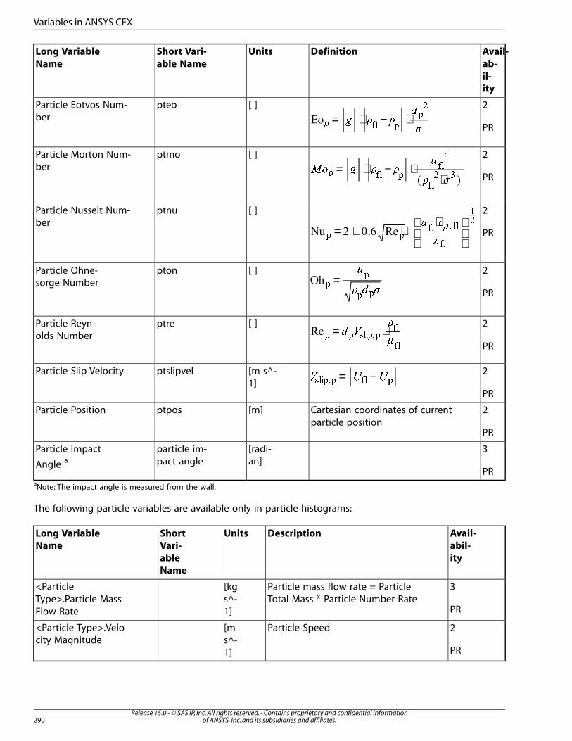
Avail-
ab-
il-
ity
DefinitionUnitsShort Vari-
able Name
Long Variable
Name
2
= ⋅ − ⋅� � ��
�� �� �
��[ ]pteoParticle Eotvos Num-
berPR
2
= ⋅ − ⋅⋅
� � �
� �� �� �
��
�
��
� �
[ ]ptmoParticle Morton Num-ber
PR
2
= + ⋅
⋅
� �
�
�� �
�� � ��
��
��
[ ]ptnuParticle Nusselt Num-ber
PR
2=
! " #$
$
$ $
[ ]ptonParticle Ohne-sorge Number
PR
2= ⋅% &
'
() ) *+,)-)
.+
.+
[ ]ptreParticle Reyn-olds Number
PR
2= −/ 0 0123454 62 4[m s^-1]
ptslipvelParticle Slip Velocity
PR
2Cartesian coordinates of currentparticle position
[m]ptposParticle Position
PR
3[radi-an]
particle im-pact angle
Particle Impact
Angle a
PRaNote: The impact angle is measured from the wall.
The following particle variables are available only in particle histograms:
Avail-
abil-
ity
DescriptionUnitsShort
Vari-
able
Name
Long Variable
Name
3Particle mass flow rate = ParticleTotal Mass * Particle Number Rate
[kgs^-1]
<ParticleType>.Particle MassFlow Rate PR
2Particle Speed[ms^-1]
<Particle Type>.Velo-city Magnitude
PR
Release 15.0 - © SAS IP, Inc. All rights reserved. - Contains proprietary and confidential informationof ANSYS, Inc. and its subsidiaries and affiliates.290
Variables in ANSYS CFX
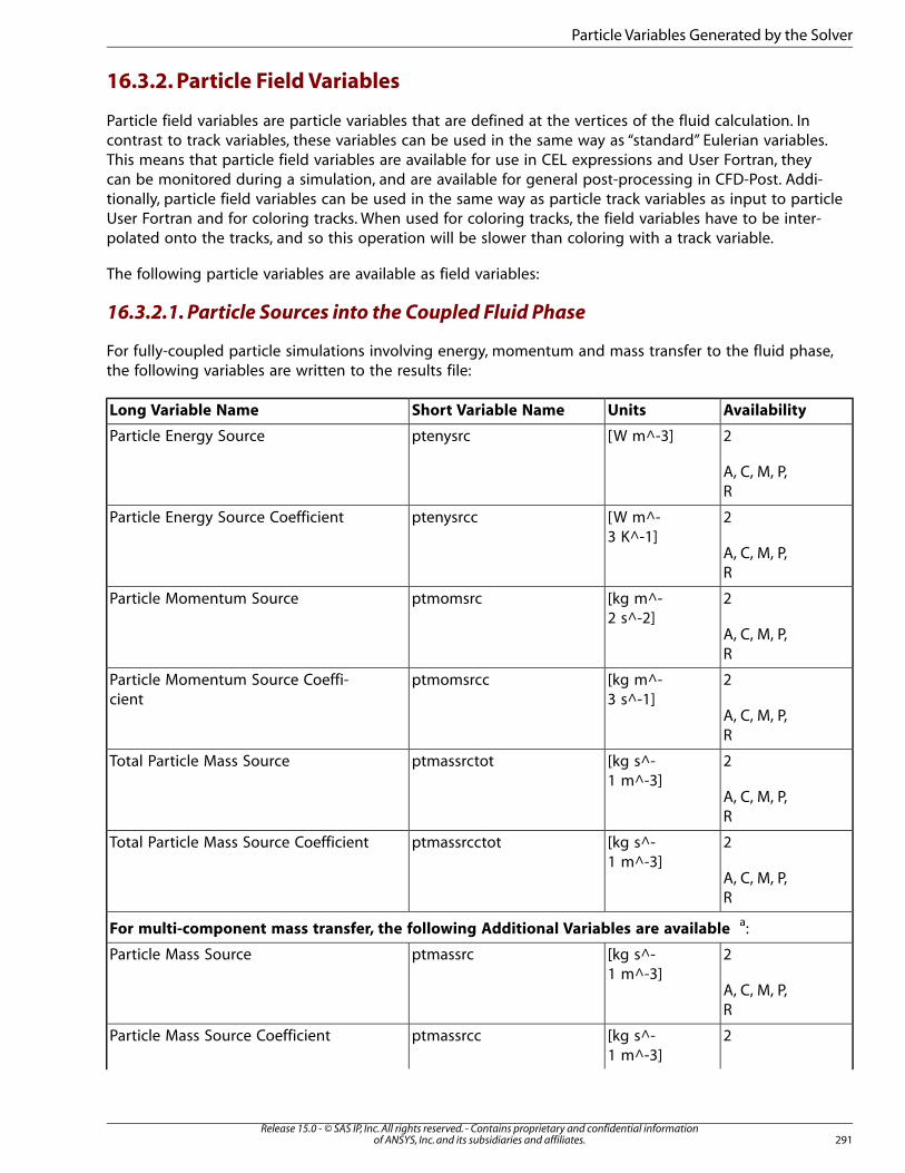
16.3.2. Particle Field Variables
Particle field variables are particle variables that are defined at the vertices of the fluid calculation. Incontrast to track variables, these variables can be used in the same way as “standard” Eulerian variables.This means that particle field variables are available for use in CEL expressions and User Fortran, theycan be monitored during a simulation, and are available for general post-processing in CFD-Post. Addi-tionally, particle field variables can be used in the same way as particle track variables as input to particleUser Fortran and for coloring tracks. When used for coloring tracks, the field variables have to be inter-polated onto the tracks, and so this operation will be slower than coloring with a track variable.
The following particle variables are available as field variables:
16.3.2.1. Particle Sources into the Coupled Fluid Phase
For fully-coupled particle simulations involving energy, momentum and mass transfer to the fluid phase,the following variables are written to the results file:
AvailabilityUnitsShort Variable NameLong Variable Name
2[W m^-3]ptenysrcParticle Energy Source
A, C, M, P,R
2[W m^-3 K^-1]
ptenysrccParticle Energy Source Coefficient
A, C, M, P,R
2[kg m^-2 s^-2]
ptmomsrcParticle Momentum Source
A, C, M, P,R
2[kg m^-3 s^-1]
ptmomsrccParticle Momentum Source Coeffi-cient
A, C, M, P,R
2[kg s^-1 m^-3]
ptmassrctotTotal Particle Mass Source
A, C, M, P,R
2[kg s^-1 m^-3]
ptmassrcctotTotal Particle Mass Source Coefficient
A, C, M, P,R
For multi-component mass transfer, the following Additional Variables are available a:
2[kg s^-1 m^-3]
ptmassrcParticle Mass Source
A, C, M, P,R
2[kg s^-1 m^-3]
ptmassrccParticle Mass Source Coefficient
291Release 15.0 - © SAS IP, Inc. All rights reserved. - Contains proprietary and confidential information
of ANSYS, Inc. and its subsidiaries and affiliates.
Particle Variables Generated by the Solver
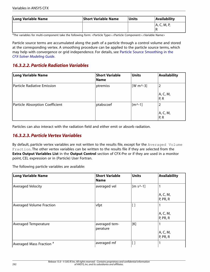
AvailabilityUnitsShort Variable NameLong Variable Name
A, C, M, P,R
aThe variables for multi-component take the following form: <Particle Type>.<Particle Component>.<Variable Name>
Particle source terms are accumulated along the path of a particle through a control volume and storedat the corresponding vertex. A smoothing procedure can be applied to the particle source terms, whichmay help with convergence or grid independence. For details, see Particle Source Smoothing in theCFX-Solver Modeling Guide.
16.3.2.2. Particle Radiation Variables
AvailabilityUnitsShort Variable
Name
Long Variable Name
2[W m^-3]ptremissParticle Radiative Emission
A, C, M,P, R
2[m^-1]ptabscoefParticle Absorption Coefficient
A, C, M,P, R
Particles can also interact with the radiation field and either emit or absorb radiation.
16.3.2.3. Particle Vertex Variables
By default, particle vertex variables are not written to the results file, except for the Averaged VolumeFraction . The other vertex variables can be written to the results file if they are selected from theExtra Output Variables List in the Output Control section of CFX-Pre or if they are used in a monitorpoint, CEL expression or in (Particle) User Fortran.
The following particle variables are available:
AvailabilityUnitsShort Variable
Name
Long Variable Name
1[m s^-1]averaged velAveraged Velocity
A, C, M,P, PR, R
1[ ]vfptAveraged Volume Fraction
A, C, M,P, PR, R
1[K]averaged tem-perature
Averaged Temperature
A, C, M,P, PR, R
1[ ]averaged mfAveraged Mass Fraction a
Release 15.0 - © SAS IP, Inc. All rights reserved. - Contains proprietary and confidential informationof ANSYS, Inc. and its subsidiaries and affiliates.292
Variables in ANSYS CFX
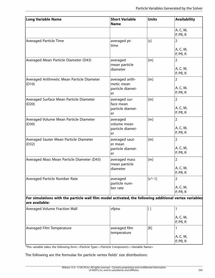
AvailabilityUnitsShort Variable
Name
Long Variable Name
A, C, M,P, PR, R
2[s]averaged pt-time
Averaged Particle Time
A, C, M,P, PR, R
2[m]averagedmean particlediameter
Averaged Mean Particle Diameter (D43)
A, C, M,P, PR, R
2[m]averaged arith-metic mean
Averaged Arithmetic Mean Particle Diameter(D10)
A, C, M,P, PR, R
particle diamet-er
2[m]averaged sur-face mean
Averaged Surface Mean Particle Diameter(D20)
A, C, M,P, PR, R
particle diamet-er
2[m]averagedvolume mean
Averaged Volume Mean Particle Diameter(D30)
A, C, M,P, PR, R
particle diamet-er
2[m]averaged saut-er mean
Averaged Sauter Mean Particle Diameter(D32)
A, C, M,P, PR, R
particle diamet-er
2[m]averaged massmean particlediameter
Averaged Mass Mean Particle Diameter (D43)
A, C, M,P, PR, R
2[s^-1]averagedparticle num-ber rate
Averaged Particle Number Rate
A, C, M,P, PR, R
For simulations with the particle wall film model activated, the following additional vertex variables
are available:
1[ ]vfptwAveraged Volume Fraction Wall
A, C, M,P, PR, R
1[K]averaged filmtemperature
Averaged Film Temperature
A, C, M,P, PR, R
aThis variable takes the following form: <Particle Type>.<Particle Component>.<Variable Name>
The following are the formulae for particle vertex fields' size distributions:
293Release 15.0 - © SAS IP, Inc. All rights reserved. - Contains proprietary and confidential information
of ANSYS, Inc. and its subsidiaries and affiliates.
Particle Variables Generated by the Solver
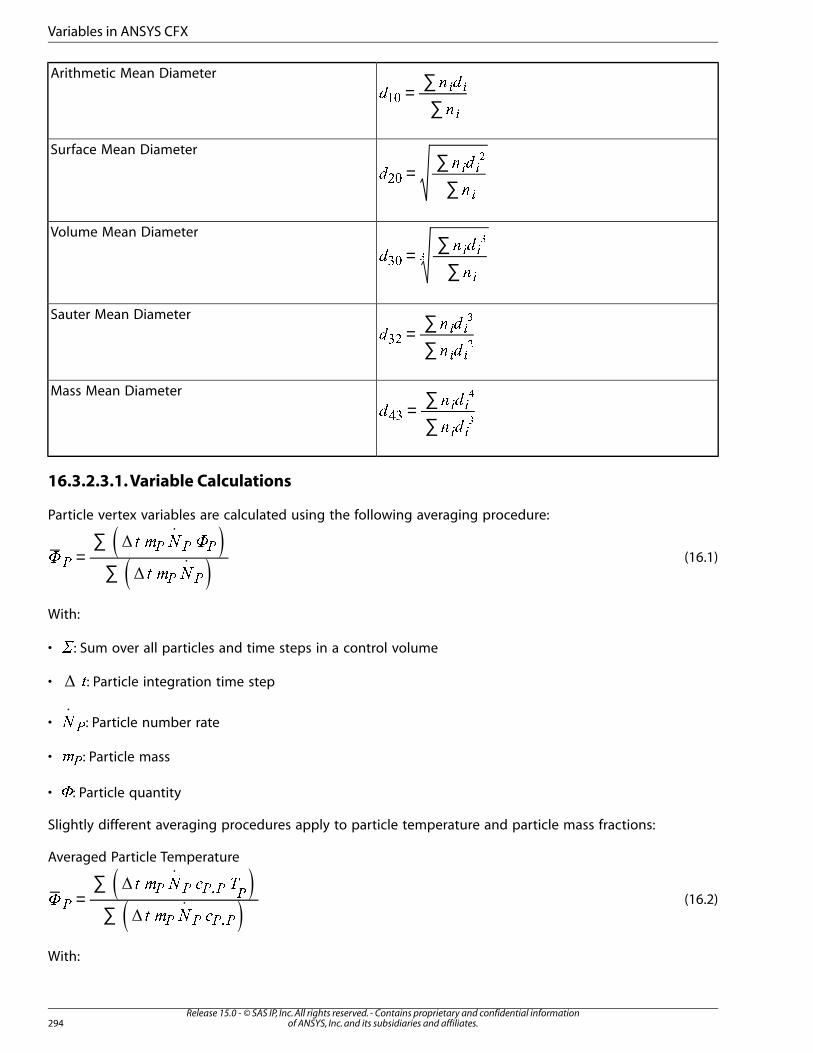
∑∑
=�� �
�
� �
�
��
Arithmetic Mean Diameter
∑∑
=�� �
�
� �
�
�
Surface Mean Diameter
∑∑
=�� �
�
��
�
�
Volume Mean Diameter
∑∑
=�� �
� �
� �
� �
��
�
�
Sauter Mean Diameter
∑∑
=�� �
� �
� �
� �
��
�
�
Mass Mean Diameter
16.3.2.3.1. Variable Calculations
Particle vertex variables are calculated using the following averaging procedure:
(16.1)∑
∑=�
! " �
! "#
# # #
# #
With:
• $: Sum over all particles and time steps in a control volume
• %: Particle integration time step
• & ': Particle number rate
• (): Particle mass
• *: Particle quantity
Slightly different averaging procedures apply to particle temperature and particle mass fractions:
Averaged Particle Temperature
(16.2)∑
∑=+
, - . / 0
, - . /1
1 1 1 1 1
1 1 1 1
2
2
With:
Release 15.0 - © SAS IP, Inc. All rights reserved. - Contains proprietary and confidential informationof ANSYS, Inc. and its subsidiaries and affiliates.294
Variables in ANSYS CFX
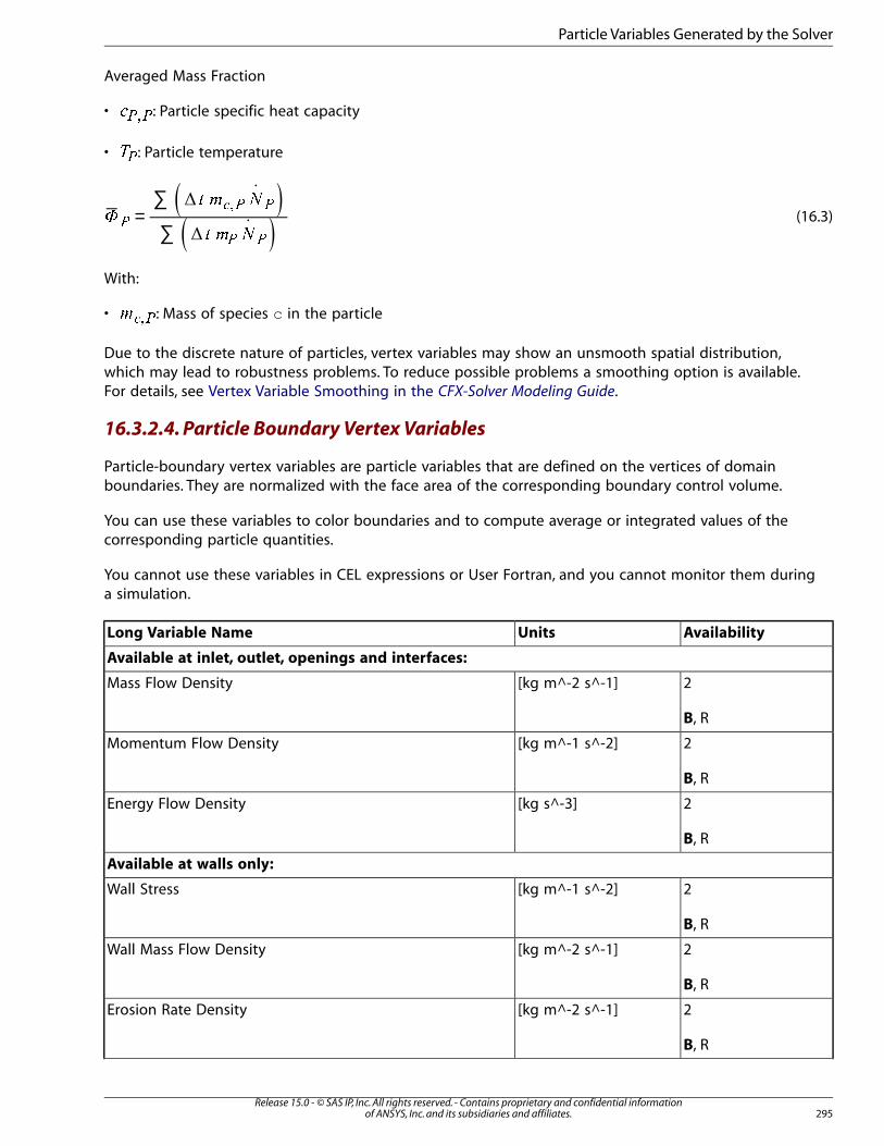
Averaged Mass Fraction
• �� �� : Particle specific heat capacity
• ��: Particle temperature
(16.3)∑
∑=�
� � �
� � �
�
With:
• � �� : Mass of species c in the particle
Due to the discrete nature of particles, vertex variables may show an unsmooth spatial distribution,which may lead to robustness problems. To reduce possible problems a smoothing option is available.For details, see Vertex Variable Smoothing in the CFX-Solver Modeling Guide.
16.3.2.4. Particle Boundary Vertex Variables
Particle-boundary vertex variables are particle variables that are defined on the vertices of domainboundaries. They are normalized with the face area of the corresponding boundary control volume.
You can use these variables to color boundaries and to compute average or integrated values of thecorresponding particle quantities.
You cannot use these variables in CEL expressions or User Fortran, and you cannot monitor them duringa simulation.
AvailabilityUnitsLong Variable Name
Available at inlet, outlet, openings and interfaces:
2[kg m^-2 s^-1]Mass Flow Density
B, R
2[kg m^-1 s^-2]Momentum Flow Density
B, R
2[kg s^-3]Energy Flow Density
B, R
Available at walls only:
2[kg m^-1 s^-2]Wall Stress
B, R
2[kg m^-2 s^-1]Wall Mass Flow Density
B, R
2[kg m^-2 s^-1]Erosion Rate Density
B, R
295Release 15.0 - © SAS IP, Inc. All rights reserved. - Contains proprietary and confidential information
of ANSYS, Inc. and its subsidiaries and affiliates.
Particle Variables Generated by the Solver
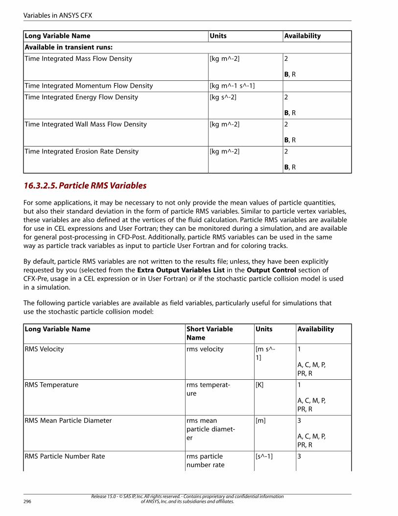
AvailabilityUnitsLong Variable Name
Available in transient runs:
2[kg m^-2]Time Integrated Mass Flow Density
B, R
[kg m^-1 s^-1]Time Integrated Momentum Flow Density
2[kg s^-2]Time Integrated Energy Flow Density
B, R
2[kg m^-2]Time Integrated Wall Mass Flow Density
B, R
2[kg m^-2]Time Integrated Erosion Rate Density
B, R
16.3.2.5. Particle RMS Variables
For some applications, it may be necessary to not only provide the mean values of particle quantities,but also their standard deviation in the form of particle RMS variables. Similar to particle vertex variables,these variables are also defined at the vertices of the fluid calculation. Particle RMS variables are availablefor use in CEL expressions and User Fortran; they can be monitored during a simulation, and are availablefor general post-processing in CFD-Post. Additionally, particle RMS variables can be used in the sameway as particle track variables as input to particle User Fortran and for coloring tracks.
By default, particle RMS variables are not written to the results file; unless, they have been explicitlyrequested by you (selected from the Extra Output Variables List in the Output Control section ofCFX-Pre, usage in a CEL expression or in User Fortran) or if the stochastic particle collision model is usedin a simulation.
The following particle variables are available as field variables, particularly useful for simulations thatuse the stochastic particle collision model:
AvailabilityUnitsShort Variable
Name
Long Variable Name
1[m s^-1]
rms velocityRMS Velocity
A, C, M, P,PR, R
1[K]rms temperat-ure
RMS Temperature
A, C, M, P,PR, R
3[m]rms meanparticle diamet-er
RMS Mean Particle Diameter
A, C, M, P,PR, R
3[s^-1]rms particlenumber rate
RMS Particle Number Rate
Release 15.0 - © SAS IP, Inc. All rights reserved. - Contains proprietary and confidential informationof ANSYS, Inc. and its subsidiaries and affiliates.296
Variables in ANSYS CFX

AvailabilityUnitsShort Variable
Name
Long Variable Name
A, C, M, P,PR, R
16.3.2.5.1. Variable Calculations
Particle RMS variables are calculated using the following procedure:
(16.4)= + ′′
= ′′ = − = −
� � �
� � � � � ����� � � �
With:
• �: Instantaneous particle quantity
• � : Average particle quantity
• ′′� : Fluctuating particle quantity
• �
: Average of square of particle quantity
• �: Square of average of particle quantity
A smoothing option, as available for particle vertex variables, is available for particle RMS variables. Fordetails, see Vertex Variable Smoothing in the CFX-Solver Modeling Guide.
16.4. Miscellaneous Variables
Variable names in bold are not output to CFD-Post.
In the Availability column:
• A number represents the user level (1 indicates that the variable appears in default lists, 2 and 3 indicate
that the variable appears in extended lists that you see when you click )
• A indicates the variable is available for mesh adaption
• C indicates the variable is available in CEL
• DT indicates the variable is available for data transfer to ANSYS
• M indicates the variable is available for monitoring
• P indicates the variable is available for particle user routine argument lists
• PR indicates the variable is available for particle results
• R indicates the variable is available to be output to the results, transient results, and backup files
• TS indicates the variable is available for transient statistics
297Release 15.0 - © SAS IP, Inc. All rights reserved. - Contains proprietary and confidential information
of ANSYS, Inc. and its subsidiaries and affiliates.
Miscellaneous Variables
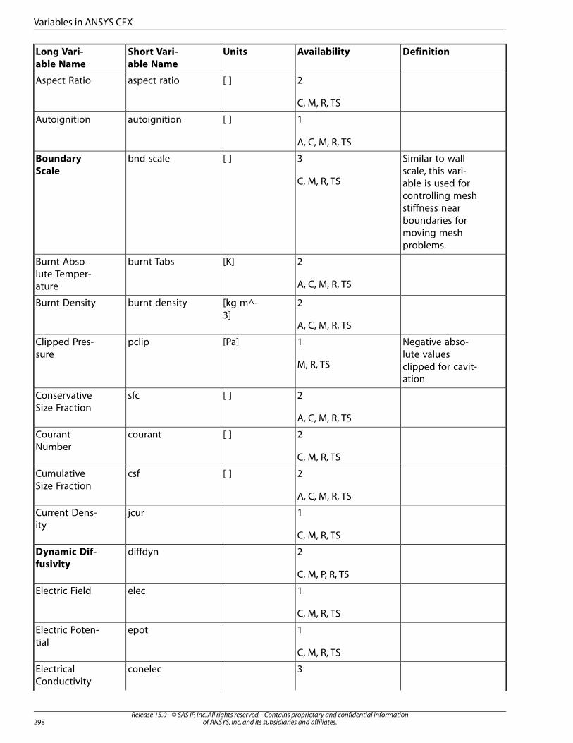
DefinitionAvailabilityUnitsShort Vari-
able Name
Long Vari-
able Name
2[ ]aspect ratioAspect Ratio
C, M, R, TS
1[ ]autoignitionAutoignition
A, C, M, R, TS
Similar to wallscale, this vari-
3
C, M, R, TS
[ ]bnd scaleBoundary
Scale
able is used forcontrolling meshstiffness nearboundaries formoving meshproblems.
2[K]burnt TabsBurnt Abso-lute Temper-ature A, C, M, R, TS
2[kg m^-3]
burnt densityBurnt Density
A, C, M, R, TS
Negative abso-lute values
1
M, R, TS
[Pa]pclipClipped Pres-sure
clipped for cavit-ation
2[ ]sfcConservativeSize Fraction
A, C, M, R, TS
2[ ]courantCourantNumber
C, M, R, TS
2[ ]csfCumulativeSize Fraction
A, C, M, R, TS
1jcurCurrent Dens-ity
C, M, R, TS
2diffdynDynamic Dif-
fusivityC, M, P, R, TS
1elecElectric Field
C, M, R, TS
1epotElectric Poten-tial
C, M, R, TS
3conelecElectricalConductivity
Release 15.0 - © SAS IP, Inc. All rights reserved. - Contains proprietary and confidential informationof ANSYS, Inc. and its subsidiaries and affiliates.298
Variables in ANSYS CFX
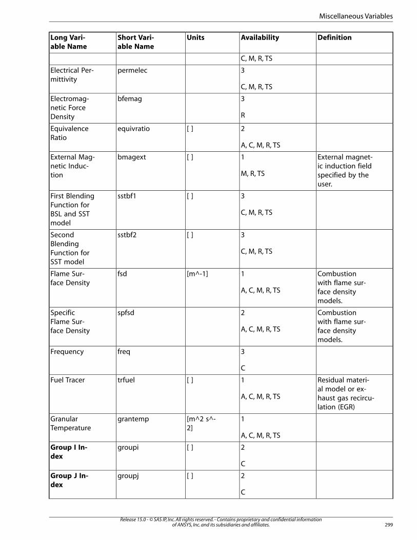
DefinitionAvailabilityUnitsShort Vari-
able Name
Long Vari-
able Name
C, M, R, TS
3permelecElectrical Per-mittivity
C, M, R, TS
3bfemagElectromag-netic ForceDensity R
2[ ]equivratioEquivalenceRatio
A, C, M, R, TS
External magnet-ic induction field
1
M, R, TS
[ ]bmagextExternal Mag-netic Induc-tion specified by the
user.
3[ ]sstbf1First BlendingFunction for
C, M, R, TSBSL and SSTmodel
3[ ]sstbf2SecondBlending
C, M, R, TSFunction forSST model
Combustionwith flame sur-
1
A, C, M, R, TS
[m^-1]fsdFlame Sur-face Density
face densitymodels.
Combustionwith flame sur-
2
A, C, M, R, TS
spfsdSpecificFlame Sur-face Density face density
models.
3freqFrequency
C
Residual materi-al model or ex-
1
A, C, M, R, TS
[ ]trfuelFuel Tracer
haust gas recircu-lation (EGR)
1[m^2 s^-2]
grantempGranularTemperature
A, C, M, R, TS
2[ ]groupiGroup I In-
dexC
2[ ]groupjGroup J In-
dexC
299Release 15.0 - © SAS IP, Inc. All rights reserved. - Contains proprietary and confidential information
of ANSYS, Inc. and its subsidiaries and affiliates.
Miscellaneous Variables
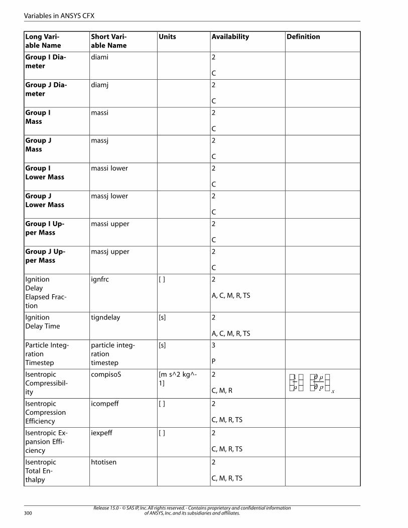
DefinitionAvailabilityUnitsShort Vari-
able Name
Long Vari-
able Name
2diamiGroup I Dia-
meterC
2diamjGroup J Dia-
meterC
2massiGroup I
MassC
2massjGroup J
MassC
2massi lowerGroup I
Lower MassC
2massj lowerGroup J
Lower MassC
2massi upperGroup I Up-
per MassC
2massj upperGroup J Up-
per MassC
2[ ]ignfrcIgnitionDelay
A, C, M, R, TSElapsed Frac-tion
2[s]tigndelayIgnitionDelay Time
A, C, M, R, TS
3[s]particle integ-rationtimestep
Particle Integ-rationTimestep P
∂∂�
�
��
�2
C, M, R
[m s^2 kg^-1]
compisoSIsentropicCompressibil-ity
2[ ]icompeffIsentropicCompressionEfficiency C, M, R, TS
2[ ]iexpeffIsentropic Ex-pansion Effi-ciency C, M, R, TS
2htotisenIsentropicTotal En-thalpy C, M, R, TS
Release 15.0 - © SAS IP, Inc. All rights reserved. - Contains proprietary and confidential informationof ANSYS, Inc. and its subsidiaries and affiliates.300
Variables in ANSYS CFX
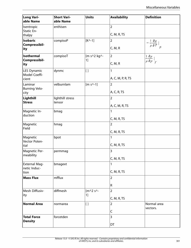
DefinitionAvailabilityUnitsShort Vari-
able Name
Long Vari-
able Name
2enthisenIsentropicStatic En-thalpy C, M, R, TS
− ∂∂�
�
��
�2
C, M, R
[K^-1] compisoPIsobaric
Compressibil-
ity
∂∂�
�
��
�2
C, M, R
[m s^2 kg^-1]
compisoTIsothermal
Compressibil-
ity
1[ ]dynmcLES DynamicModel Coeffi-cient A, C, M, P, R, TS
2[m s^-1]velburnlamLaminarBurning Velo-city A, C, R, TS
2lighthill stresstensor
Lighthill
StressA, C, M, R, TS
1bmagMagnetic In-duction
C, M, R, TS
2hmagMagneticField
C, M, R, TS
1bpotMagneticVector Poten-tial C, M, R, TS
3permmagMagnetic Per-meability
C, M, R, TS
1bmagextExternal Mag-netic Induc-tion C, M, R, TS
2mffluxMass Flux
R
2[m^2 s^-1]
diffmeshMesh Diffusiv-ity
C, M, R, TS
Normal areavectors.
2
C
[ ]normareaNormal Area
3forcetdenTotal Force
DensityDT
301Release 15.0 - © SAS IP, Inc. All rights reserved. - Contains proprietary and confidential information
of ANSYS, Inc. and its subsidiaries and affiliates.
Miscellaneous Variables
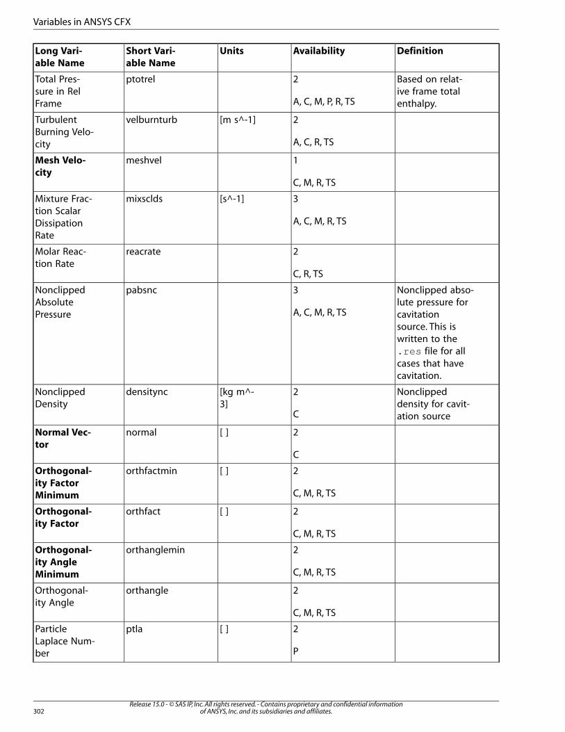
DefinitionAvailabilityUnitsShort Vari-
able Name
Long Vari-
able Name
Based on relat-ive frame totalenthalpy.
2
A, C, M, P, R, TS
ptotrelTotal Pres-sure in RelFrame
2[m s^-1]velburnturbTurbulentBurning Velo-city A, C, R, TS
1meshvelMesh Velo-
cityC, M, R, TS
3[s^-1]mixscldsMixture Frac-tion Scalar
A, C, M, R, TSDissipationRate
2reacrateMolar Reac-tion Rate
C, R, TS
Nonclipped abso-lute pressure for
3
A, C, M, R, TS
pabsncNonclippedAbsolutePressure cavitation
source. This iswritten to the.res file for allcases that havecavitation.
Nonclippeddensity for cavit-ation source
2
C
[kg m^-3]
densityncNonclippedDensity
2[ ]normalNormal Vec-
torC
2[ ]orthfactminOrthogonal-
ity Factor
Minimum C, M, R, TS
2[ ]orthfact Orthogonal-
ity FactorC, M, R, TS
2orthangleminOrthogonal-
ity Angle
Minimum C, M, R, TS
2orthangleOrthogonal-ity Angle
C, M, R, TS
2[ ]ptlaParticleLaplace Num-ber P
Release 15.0 - © SAS IP, Inc. All rights reserved. - Contains proprietary and confidential informationof ANSYS, Inc. and its subsidiaries and affiliates.302
Variables in ANSYS CFX
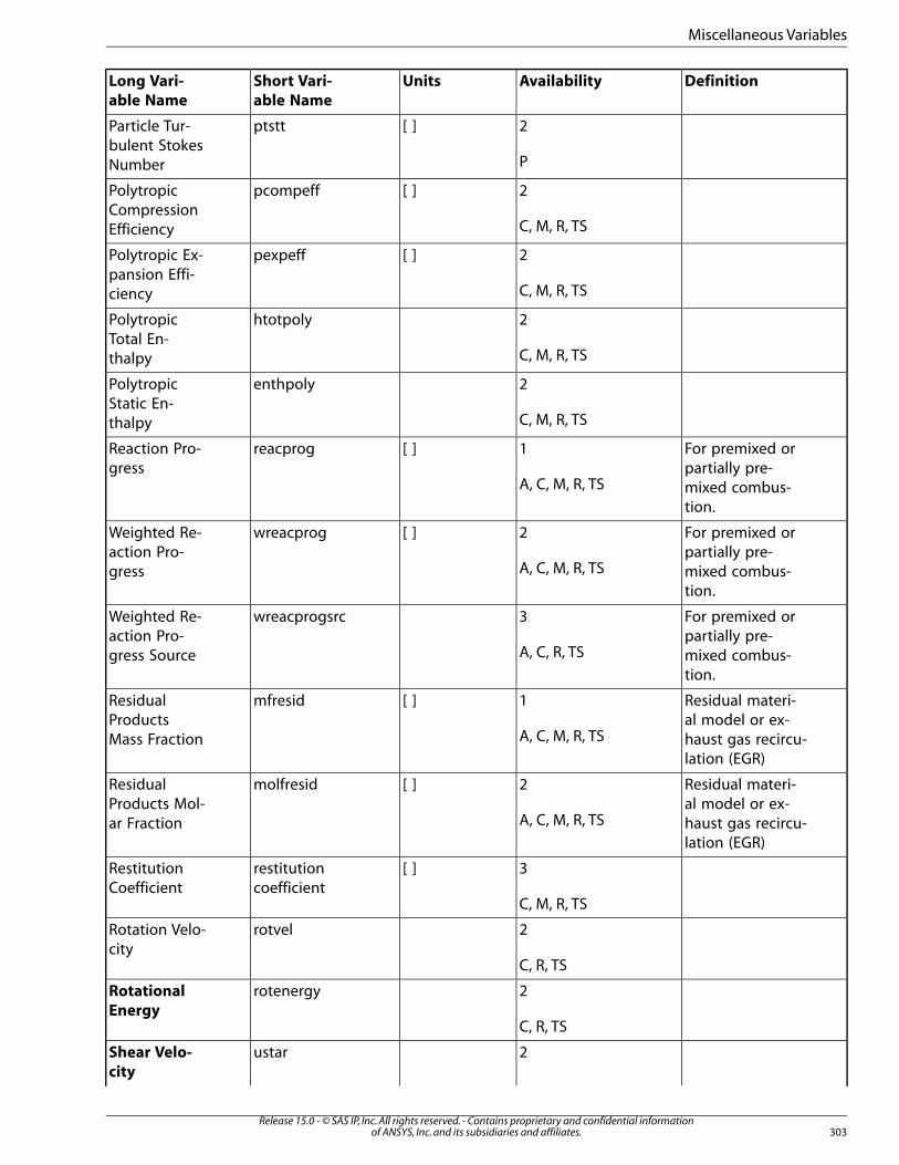
DefinitionAvailabilityUnitsShort Vari-
able Name
Long Vari-
able Name
2[ ]ptsttParticle Tur-bulent StokesNumber P
2[ ]pcompeffPolytropicCompressionEfficiency C, M, R, TS
2[ ]pexpeffPolytropic Ex-pansion Effi-ciency C, M, R, TS
2htotpolyPolytropicTotal En-thalpy C, M, R, TS
2enthpolyPolytropicStatic En-thalpy C, M, R, TS
For premixed orpartially pre-
1
A, C, M, R, TS
[ ]reacprogReaction Pro-gress
mixed combus-tion.
For premixed orpartially pre-
2
A, C, M, R, TS
[ ]wreacprogWeighted Re-action Pro-gress mixed combus-
tion.
For premixed orpartially pre-
3
A, C, R, TS
wreacprogsrcWeighted Re-action Pro-gress Source mixed combus-
tion.
Residual materi-al model or ex-
1
A, C, M, R, TS
[ ]mfresidResidualProductsMass Fraction haust gas recircu-
lation (EGR)
Residual materi-al model or ex-
2
A, C, M, R, TS
[ ]molfresidResidualProducts Mol-ar Fraction haust gas recircu-
lation (EGR)
3[ ]restitutioncoefficient
RestitutionCoefficient
C, M, R, TS
2rotvelRotation Velo-city
C, R, TS
2rotenergyRotational
EnergyC, R, TS
2ustarShear Velo-
city
303Release 15.0 - © SAS IP, Inc. All rights reserved. - Contains proprietary and confidential information
of ANSYS, Inc. and its subsidiaries and affiliates.
Miscellaneous Variables
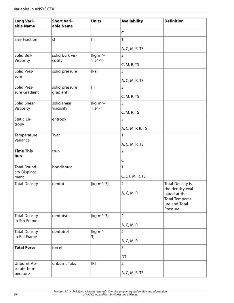
DefinitionAvailabilityUnitsShort Vari-
able Name
Long Vari-
able Name
C
1[ ]sfSize Fraction
A, C, M, R, TS
3[kg m^-1 s^-1]
solid bulk vis-cosity
Solid BulkViscosity
C, M, R, TS
3[Pa]solid pressureSolid Pres-sure
A, C, M, R, TS
3[ ]solid pressuregradient
Solid Pres-sure Gradient
C, M, R, TS
3[kg m^-1 s^-1]
solid shearviscosity
Solid ShearViscosity
C, M, R, TS
3entropyStatic En-tropy
A, C, M, P, R, TS
1TvarTemperatureVariance
A, C, M, R, TS
2trunTime This
RunC
1bnddisptotTotal Bound-ary Displace-ment C, DT, M, R, TS
Total Density isthe density eval-
2
A, C, M, R
[kg m^-3]dentotTotal Density
uated at theTotal Temperat-ure and TotalPressure.
2[kg m^-3]dentotstnTotal Densityin Stn Frame
A, C, M, R
2[kg m^-3]
dentotrelTotal Densityin Rel Frame
A, C, M, R
3forcetTotal Force
DT
2[K]unburnt TabsUnburnt Ab-solute Tem-perature A, C, M, R, TS
Release 15.0 - © SAS IP, Inc. All rights reserved. - Contains proprietary and confidential informationof ANSYS, Inc. and its subsidiaries and affiliates.304
Variables in ANSYS CFX
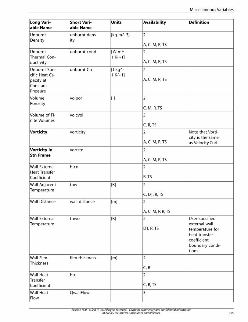
DefinitionAvailabilityUnitsShort Vari-
able Name
Long Vari-
able Name
2[kg m^-3]unburnt dens-ity
UnburntDensity
A, C, M, R, TS
2[W m^-1 K^-1]
unburnt condUnburntThermal Con-ductivity A, C, M, R, TS
2[J kg^-1 K^-1]
unburnt CpUnburnt Spe-cific Heat Ca-
A, C, M, R, TSpacity atConstantPressure
2[ ]volporVolumePorosity
C, M, R, TS
3volcvolVolume of Fi-nite Volumes
C, R, TS
Note that Vorti-city is the sameas Velocity.Curl.
2
A, C, M, R, TS
vorticityVorticity
2vortstnVorticity in
Stn FrameA, C, M, R, TS
2htcoWall ExternalHeat TransferCoefficient R, TS
2[K]tnwWall AdjacentTemperature
C, DT, R, TS
2[m]wall distanceWall Distance
A, C, M, P, R, TS
User-specifiedexternal wall
2
DT, R, TS
[K]tnwoWall ExternalTemperature
temperature forheat transfercoefficientboundary condi-tions.
2[m]film thicknessWall FilmThickness
C, R
2htcWall HeatTransferCoefficient C, R, TS
3QwallFlowWall HeatFlow
305Release 15.0 - © SAS IP, Inc. All rights reserved. - Contains proprietary and confidential information
of ANSYS, Inc. and its subsidiaries and affiliates.
Miscellaneous Variables

DefinitionAvailabilityUnitsShort Vari-
able Name
Long Vari-
able Name
C, DT, R, TS
2nwallvelWall NormalVelocity
C, R, TS
3wall scaleWall Scale
R, M, TS
3waveloWavelengthin Vacuum
C
3wavenoWavenumberin Vacuum
C
2[m^-3]spdropnNormalizedDroplet Num-ber C, M, R, TS
1spdropDroplet Num-ber
C, M, R, TS
1dynamic bulkviscosity
Dynamic BulkViscosity
A, C, M, R, TS
2[ ]vftTotal MUSIGVolume Frac-tion A, C, M, R, TS
2[ ]vfsSmoothed
Volume
Fraction A, C, M, R, TS
Temperatureabove saturation
3
C
TsuperheatTemperatureSuperheating
Temperature be-low saturation
3
C
TsubcoolTemperatureSubcooling
Release 15.0 - © SAS IP, Inc. All rights reserved. - Contains proprietary and confidential informationof ANSYS, Inc. and its subsidiaries and affiliates.306
Variables in ANSYS CFX
Chapter 17: Power Syntax in ANSYS CFX
Programming constructs can be used within CCL for advanced usage. Rather than invent a new language,CCL takes advantage of the full range of capabilities and resources from an existing programming lan-guage, Perl. Perl statements can be embedded in between lines of simple syntax, providing capabilitiessuch as loops, logic, and much, much more with any CCL input file.
A line of Power Syntax is identified in a CCL file by an exclamation mark (! ) in the first column of a line.In between Perl lines, simple syntax lines may refer to Perl variables and lists.
A wide range of additional functionality is made available to expert users with the use of Power Syntaxincluding:
• Loops
• Logic and control structures
• Lists and arrays
• Subroutines with argument handling (useful for defining commonly re-used plots and procedures)
• Basic I/O processing
• System functions
• Many other procedures (Object programming, World Wide Web access, simple embedded graphical userinterfaces).
Any of the above may be included in a CCL input file or CFD-Post Session file.
Important
You should be wary when entering certain expressions because Power Syntax uses Perl
mathematical operators. For example, in CEL,� is represented as 2^2 , but in Perl, it would
be written 2**2 . If you are unsure about the validity of an operator, you should check a Perlreference guide.
There are many good reference books on Perl. Two examples are Learning Perl (ISBN 1-56592-042-2) and Programming Perl (ISBN 1-56592-149-6) from the O’Reilly series.
This chapter describes:17.1. Examples of Power Syntax17.2. Predefined Power Syntax Subroutines
307Release 15.0 - © SAS IP, Inc. All rights reserved. - Contains proprietary and confidential information
of ANSYS, Inc. and its subsidiaries and affiliates.
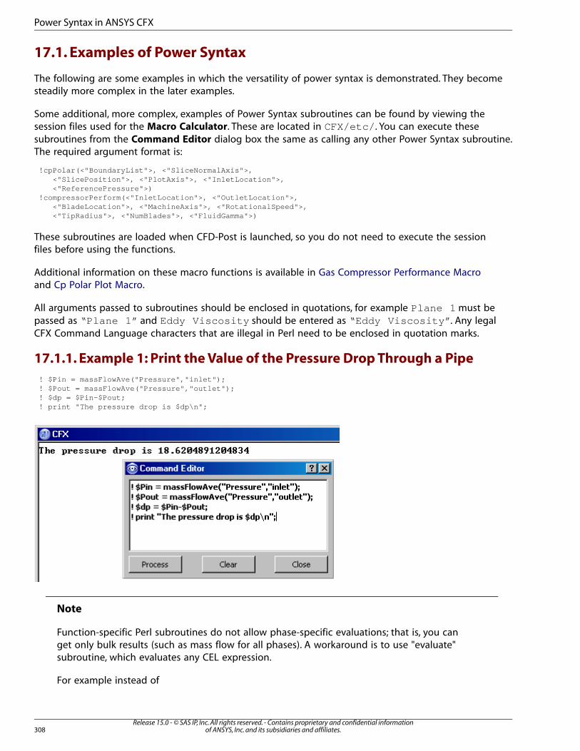
17.1. Examples of Power Syntax
The following are some examples in which the versatility of power syntax is demonstrated. They becomesteadily more complex in the later examples.
Some additional, more complex, examples of Power Syntax subroutines can be found by viewing thesession files used for the Macro Calculator. These are located in CFX/etc/ . You can execute thesesubroutines from the Command Editor dialog box the same as calling any other Power Syntax subroutine.The required argument format is:
!cpPolar(<"BoundaryList">, <"SliceNormalAxis">, <"SlicePosition">, <"PlotAxis">, <"InletLocation">, <"ReferencePressure">)!compressorPerform(<"InletLocation">, <"OutletLocation">, <"BladeLocation">, <"MachineAxis">, <"RotationalSpeed">, <"TipRadius">, <"NumBlades">, <"FluidGamma">)
These subroutines are loaded when CFD-Post is launched, so you do not need to execute the sessionfiles before using the functions.
Additional information on these macro functions is available in Gas Compressor Performance Macroand Cp Polar Plot Macro.
All arguments passed to subroutines should be enclosed in quotations, for example Plane 1 must bepassed as “ Plane 1 ” and Eddy Viscosity should be entered as “ Eddy Viscosity ” . Any legalCFX Command Language characters that are illegal in Perl need to be enclosed in quotation marks.
17.1.1. Example 1: Print the Value of the Pressure Drop Through a Pipe
! $Pin = massFlowAve("Pressure","inlet");! $Pout = massFlowAve("Pressure","outlet");! $dp = $Pin-$Pout;! print "The pressure drop is $dp\n";
Note
Function-specific Perl subroutines do not allow phase-specific evaluations; that is, you canget only bulk results (such as mass flow for all phases). A workaround is to use "evaluate"subroutine, which evaluates any CEL expression.
For example instead of
Release 15.0 - © SAS IP, Inc. All rights reserved. - Contains proprietary and confidential informationof ANSYS, Inc. and its subsidiaries and affiliates.308
Power Syntax in ANSYS CFX
! $val = massFlow("Inlet", "Water") # Does NOT work
you need to use:
! ($val, $units) = evaluate( "Water.massFlow()\@Inlet");
17.1.2. Example 2: Using a for Loop
This example demonstrates using Power Syntax that wraps a for loop around some CCL Objectdefinitions to repetitively change the visibility on the outer boundaries.
# Make the outer boundaries gradually transparent in# the specified number of steps.!$numsteps = 10;!for ($i=0; $i < $numsteps; $i++) { ! $trans = ($i+1)/$numsteps; BOUNDARY:in Visibility = 1 Transparency = $trans END BOUNDARY:out Visibility = 1 Transparency = $trans END BOUNDARY:Default Visibility = 1 Transparency = $trans END!}
The first line of Power Syntax simply defines a scalar variable called numsteps . Scalar variables (thatis, simple single-valued variables) begin with a $ symbol in Perl. The next line defines a for loop thatincrements the variable i up to numsteps . Next, you determine the fraction you are along in the loopand assign it to the variable trans . The object definitions then use trans to set their transparencyand then repeat. Note how Perl variables can be directly embedded into the object definitions. The finalline of Power Syntax (!} ) closes the for loop.
Note
Function-specific Perl subroutines do not allow phase-specific evaluations; that is, you canget only bulk results (such as mass flow for all phases). A workaround is to use "evaluate"subroutine, which evaluates any CEL expression.
For example instead of
! $val = massFlow("Inlet", "Water") # Does NOT work
you need to use:
! ($val, $units) = evaluate( "Water.massFlow()\@Inlet");
17.1.3. Example 3: Creating a Simple Subroutine
The following example defines a simple subroutine to make two planes at specified locations. Thesubroutine will be used in the next example.
!sub makePlanes { PLANE:plane1 Option = Point and Normal
309Release 15.0 - © SAS IP, Inc. All rights reserved. - Contains proprietary and confidential information
of ANSYS, Inc. and its subsidiaries and affiliates.
Examples of Power Syntax

Point = 0.09,0,-0.03 Normal = 1,0,0 Draw Lines = On Line Color = 1,0,0 Color Mode = Variable Color Variable = Pressure Range = Local END PLANE:plane2 Option = Point and Normal Point = 0.08,-0.038,-0.0474 Normal = 1,0,0 Draw Faces = Off Draw Lines = On Line Color = 0,1,0 END!}
Although this subroutine is designed for use with the next example, you can execute it on its own bytyping !makePlanes(); in the Command Editor dialog box.
17.1.4. Example 4: Creating a Complex Quantitative Subroutine
This example is a complex quantitative subroutine that takes slices through the manifold geometry, asshown below, compares the mass flow through the two sides of the initial branch, and computes thepressure drop through to the four exit locations.
! sub manifoldCalcs{# call the previously defined subroutine (Example 3) make the# upstream and downstream cutting planes! makePlanes();## Bound the two planes so they each just cut one side of the branch.PLANE:plane1Plane Bound = CircularBound Radius = 0.025ENDPLANE:plane2Plane Bound = CircularBound Radius = 0.025END# Calculate mass flow through each using the predefined# 'evaluate' Power Syntax subroutine and output the results
Release 15.0 - © SAS IP, Inc. All rights reserved. - Contains proprietary and confidential informationof ANSYS, Inc. and its subsidiaries and affiliates.310
Power Syntax in ANSYS CFX
! ($mass1, $mfunits) = evaluate( "massFlow()\@plane1" );! ($mass2) = evaluate( "massFlow()\@plane2" );! $sum = $mass1+$mass2;! print "Mass flow through branch 1 = $mass1 [$mfunits]\n";! print "Mass flow through branch 2 = $mass2 [$mfunits]\n";! print "Total = $sum [$mfunits]\n";# Now calculate pressure drops and mass flows through the exits# calculate the average pressure at the inlet!($Pin, $punits) = evaluate( "massFlowAve(Pressure)\@in1" );# Set-up an array that holds the approximate X location of each# of the 4 exits. We then loop over the array to move the outlet# plane and re-do the pressure drop calculation at each exit.! @Xlocs = (0.15,0.25,0.35,0.45);! $sum = 0;! for ($i=0;$i<4;$i++) {PLANE:outlet Option = Point and Normal Normal = 0,-1,-1 Point = $Xlocs[$i],-0.06,-0.2 Plane Bound = Circular Bound Radius = 0.05END! ($Pout, $punits) = evaluate( "massFlowAve(Pressure)\@outlet" );! ($massFl) = evaluate( "massFlow()\@outlet" );! $sum += $massFl;! $Dp = $Pin-$Pout;! $ii = $i+1;! print "At outlet \#$ii: Dp=$Dp [$punits], Mass Flow=$massFl [$mfunits]\n";! } # end loop! print "Total Mass Flow = $sum [$mfunits]\n";!} # end subroutine
After processing these commands to define the subroutine, you can execute it, in the same way as anyother subroutine, by typing !manifoldCalcs(); in the Command Editor dialog box.
17.2. Predefined Power Syntax Subroutines
CFD-Post provides predefined subroutines that add Power Syntax functionality. You can view a list ofthese subroutines by entering !showSubs(); in the Command Editor dialog box. The list is printedto the console window. The list shows all currently loaded subroutines, so it will include any customsubroutines that you have processed in the Command Editor dialog box.
These subroutines provide access to the quantitative functionality of CFD-Post. Most of these routinesprovide results in a single return value. For example, if the Perl variable $verbose = 1 , then theresult is also printed to the screen. Information on the calculations performed by the subroutines isavailable. For details, see Function Selection.
The following sections describe these predefined subroutines:
• Power Syntax Subroutine Descriptions (p. 311)
• Power Syntax Usage (p. 312)
• Power Syntax Subroutines (p. 312)
17.2.1. Power Syntax Subroutine Descriptions
In the next section, each subroutine will appear in the following format:
311Release 15.0 - © SAS IP, Inc. All rights reserved. - Contains proprietary and confidential information
of ANSYS, Inc. and its subsidiaries and affiliates.
Predefined Power Syntax Subroutines
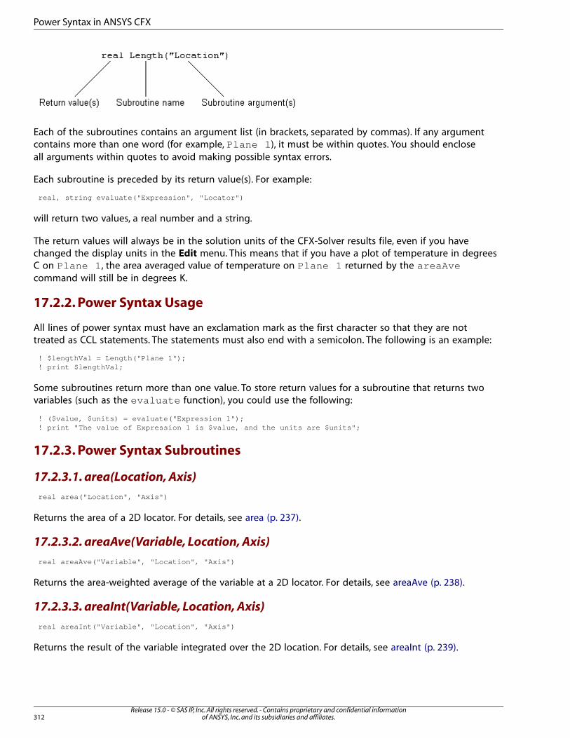
Each of the subroutines contains an argument list (in brackets, separated by commas). If any argumentcontains more than one word (for example, Plane 1 ), it must be within quotes. You should encloseall arguments within quotes to avoid making possible syntax errors.
Each subroutine is preceded by its return value(s). For example:
real, string evaluate("Expression", "Locator")
will return two values, a real number and a string.
The return values will always be in the solution units of the CFX-Solver results file, even if you havechanged the display units in the Edit menu. This means that if you have a plot of temperature in degreesC on Plane 1 , the area averaged value of temperature on Plane 1 returned by the areaAvecommand will still be in degrees K.
17.2.2. Power Syntax Usage
All lines of power syntax must have an exclamation mark as the first character so that they are nottreated as CCL statements. The statements must also end with a semicolon. The following is an example:
! $lengthVal = Length("Plane 1");! print $lengthVal;
Some subroutines return more than one value. To store return values for a subroutine that returns twovariables (such as the evaluate function), you could use the following:
! ($value, $units) = evaluate("Expression 1");! print "The value of Expression 1 is $value, and the units are $units";
17.2.3. Power Syntax Subroutines
17.2.3.1. area(Location, Axis)
real area("Location", "Axis")
Returns the area of a 2D locator. For details, see area (p. 237).
17.2.3.2. areaAve(Variable, Location, Axis)
real areaAve("Variable", "Location", "Axis")
Returns the area-weighted average of the variable at a 2D locator. For details, see areaAve (p. 238).
17.2.3.3. areaInt(Variable, Location, Axis)
real areaInt("Variable", "Location", "Axis")
Returns the result of the variable integrated over the 2D location. For details, see areaInt (p. 239).
Release 15.0 - © SAS IP, Inc. All rights reserved. - Contains proprietary and confidential informationof ANSYS, Inc. and its subsidiaries and affiliates.312
Power Syntax in ANSYS CFX
17.2.3.4. ave(Variable, Location)
real ave("Variable", "Location")
Returns the arithmetic average of the variable at a location. For details, see ave (p. 240).
17.2.3.5. calcTurboVariables()
void calcTurboVariables()
Calculates all 'extra' turbo variables. (Works only in turbo mode.)
17.2.3.6. calculate(function,...)
real calculate(function,...)
Evaluates the named function with the supplied argument list, and returns the float result. The functionname is a required argument, which can be followed by a variable length list of arguments.
17.2.3.7. calculateUnits(function,...)
string,string calculateUnits(function,...)
Evaluates the named function with the supplied argument list, and returns the value and units.
17.2.3.8. collectTurboInfo()
This is an internal subroutine that is used only to initialize report templates.
17.2.3.9. comfortFactors()
This is an internal subroutine that is used only to initialize report templates.
17.2.3.10. compressorPerform(Location, Location, Location, Var, Args)
This is a special macro; for details, see Gas Compressor Performance Macro. For example:
compressorPerform("Inlet", "Outlet", "Blade", "X", 600, 0.03, 10, 1.2)
17.2.3.11. compressorPerformTurbo()
This is an internal subroutine that is used only to initialize report templates.
17.2.3.12. copyFile(FromPath, ToPath)
void copyFile("FromPath", "ToPath")
A utility function for copying files.
17.2.3.13. count(Location)
real count("Location")
Returns the number of nodes on the location. For details, see count (p. 241).
17.2.3.14. countTrue(Expression, Location)
real countTrue("Expression", "Location")
313Release 15.0 - © SAS IP, Inc. All rights reserved. - Contains proprietary and confidential information
of ANSYS, Inc. and its subsidiaries and affiliates.
Predefined Power Syntax Subroutines
Returns the number of mesh nodes on the specified region that evaluate to “true”, where true meansgreater than or equal to 0.5. "Expression" should contain one of the logical operators =, >, <, <=,or >=. The countTrue function is valid for 1D, 2D, and 3D locations. For details, see countTrue (p. 242).
17.2.3.15. cpPolar(Location, Var, Arg, Var, Location, Arg)
This is a special macro; for details, see Cp Polar Plot Macro. For example:
cpPolar("Plane 1", "Y", 0.3, "X", "Inlet", 10000)
17.2.3.16. evaluate(Expression)
real,string evaluate("Expression")
Returns the value of the expression and the units. Only one expression can be evaluated each time thesubroutine is executed. The main advantage of using evaluate is that it takes any CEL expression.This means that you do not have to learn any other quantitative power syntax routines described inthis section. Also, evaluate will return the result units in addition to the value.
An example is:
evaluate("areaAve(Velocity v)\@Location 1")
In this case, another subroutine is evaluated. The evaluate command takes an any expression as theargument, or more precisely, any expression that resolves to a quantity. This means that you cannotuse:
"2*Pressure"
but you can use:
"2*minVal(Pressure)\@locator 1"
or
"100 [m]"
This is simply an alternative way of typing:
! $myVal = 2 * minVal("Pressure", "Location");
The reason that the @ is escaped calling evaluate() is to avoid Perl treating it as a special character.
17.2.3.17. evaluateInPreferred(Expression)
real,string evaluateInPreferred("Expression")
Returns the value of the expression in your preferred units. Preferred units are the units of the data thatCFD-Post uses when information is displayed to you and are the default units when you enter information(as contrasted with units of the data that are stored in results files). Use the Edit > Options > Common
> Units dialog box to set your preferred units.
17.2.3.18. exprExists(Expression)
bool exprExists("Expression")
Returns true if an expression with this name exists; false otherwise.
Release 15.0 - © SAS IP, Inc. All rights reserved. - Contains proprietary and confidential informationof ANSYS, Inc. and its subsidiaries and affiliates.314
Power Syntax in ANSYS CFX
17.2.3.19. fanNoiseDefault()
This is an internal subroutine that is used only to initialize report templates.
17.2.3.20. fanNoise()
This is an internal subroutine that is used only to initialize report templates.
17.2.3.21. force(Location, Axis)
real force("Location", "Axis")
Returns the force on a 2D locator. For details, see force (p. 242).
17.2.3.22. forceNorm(Location, Axis)
real forceNorm("Location", "Axis")
Returns the per unit width force on a line in the direction of the specified axis. It is available only for apolyline created by intersecting a locator on a boundary. For details, see forceNorm (p. 243).
17.2.3.23. getBladeForceExpr()
This is an internal subroutine that is used only to initialize report templates.
17.2.3.24. getBladeTorqueExpr()
This is an internal subroutine that is used only to initialize report templates.
17.2.3.25. getCCLState()
This is an internal debugging call.
17.2.3.26. getChildrenByCategory(Category)
string getChildrenByCategory("Category")
Returns the children of an object that belong to the specified category in a comma-separated list. Eachobject type (for example, a PLANE) can have multiple categories associated with it such as "geometry","surface", and so on). Categories are specified in <CFXROOT>/etc/CFXPostRules.ccl .
For example, to get a comma-separated list of all surfaces in a state at the top level (that is, not sub-objects of other objects):
! $surfaces = getChildrenByCategory("/", "surface" );
Use 'split "," ' to convert the string into an array of strings.
17.2.3.27. getChildren(Object Name, Child Type)
string getChildren("Object Name", "Child Type")
Returns the children of an object in a comma-separated list. If Child Type is not an empty string,this subroutine return only children of the specified type.
315Release 15.0 - © SAS IP, Inc. All rights reserved. - Contains proprietary and confidential information
of ANSYS, Inc. and its subsidiaries and affiliates.
Predefined Power Syntax Subroutines
17.2.3.28. getExprOnLocators()
This is an internal subroutine that is used only to initialize report templates.
17.2.3.29. getExprString(Expression)
string getExprString("Expression")
Returns the value and the units of the expression in the form “value units”. For example: “100 m”.
17.2.3.30. getExprVal(Expression)
real getExprVal("Expression")
Returns only the "value" portion of the expression (units are not included).
17.2.3.31. getObjectName(Object Path)
string getObjectName("Object Path")
Extracts the name of an object from its full path. For example:
!string = getObjectName("/USER SURFACE:User Surface 1")
returns "User Surface 1". This is the form needed for evaluating a CEL expression.
17.2.3.32. getParameterInfo(Object Name, Parameter Name, Info Type)
string getParameterInfo("Object Name", "Parameter Name", "Info Type")
Returns the requested information for a parameter of an object. Object Name returns the name orpath of an object; "/" or an empty string specifies the root.Parameter Name returns the name of theparameter. Info Type returns the type of data requested; this can be one of "type", "value", "defaultvalue", or "allowed values". For example:
! $info = getParameterInfo("/USER DEFINED/POINT:Point 1", "Symbol Size", "default value");! print "getParameterInfo returned=$info\n";
prints:
getParameterInfo returned=2.5
17.2.3.33. getParameters(Object Name)
string getParameters("Object Name")
Returns the parameters of an object in a comma-separated list. Use 'split "," ' to convert the stringinto an array of strings.
17.2.3.34. getTempDirectory()
string getTempDirectory()
Returns the temporary directory path.
17.2.3.35. getType(Object Name)
string getType("Object Name")
Returns the object type.
Release 15.0 - © SAS IP, Inc. All rights reserved. - Contains proprietary and confidential informationof ANSYS, Inc. and its subsidiaries and affiliates.316
Power Syntax in ANSYS CFX
17.2.3.36. getValue(Object Name, Parameter Name)
string getValue("Object Name", "Parameter Name")
Takes a CCL object and parameter name and returns the value of the parameter.
Returns the value stored in Parameter Name .
17.2.3.36.1. Example
1. Create a text object called Text 1.
2. In the Text String box, enter Here is a text string .
3. Click Apply to create the text object.
4. In the Command Editor dialog box, enter the following:
!string = getValue( "/TEXT:Text 1/TEXT ITEM: Text Item 1", "Text String");! print $string;
5. Click Process, and the string will be printed to your terminal window.
The same procedure can be carried out for any object.
17.2.3.37. getViewArea()
string,string getViewArea()
Calculates the area of the scene projected in the view direction. Returns the area and the units in anarray of strings.
17.2.3.38. isCategory(Object Name, Category)
bool isCategory("Object Name", "Category")
A return of 1 indicates that the object matches the passed category; 0 otherwise. Categories are specifiedin <CFXROOT>/etc/CFXPostRules.ccl .
For example, the following prints "Plane 1 is a surface":
! if( isCategory( "Plane 1", "surface" )) { ! print "Plane 1 is a surface\n"; ! }
17.2.3.39. Length(Location)
real Length("Location")
Returns the length of a line locator. For details, see length (p. 244).
Note
While using this function in Power Syntax the leading character is capitalized to avoid con-fusion with the Perl internal command “length.”
317Release 15.0 - © SAS IP, Inc. All rights reserved. - Contains proprietary and confidential information
of ANSYS, Inc. and its subsidiaries and affiliates.
Predefined Power Syntax Subroutines
17.2.3.40. lengthAve(Variable, Location)
real lengthAve("Variable", "Location")
Returns the length-based average of the variable on the line locator. For details, see lengthAve (p. 245).
17.2.3.41. lengthInt(Variable, Location)
real lengthInt("Variable", "Location")
Returns the length-based integral of the variable on the line locator. For details, see lengthInt (p. 246).
17.2.3.42. liquidTurbPerformTurbo()
This is an internal subroutine that is used only to initialize report templates.
17.2.3.43. liquidTurbPerform()
This is an internal subroutine that is used only to initialize report templates.
17.2.3.44. massFlow(Location)
real massFlow("Location")
Returns the mass flow through the 2D locator. For details, see massFlow (p. 246).
17.2.3.45. massFlowAve(Variable, Location)
real massFlowAve("Variable","Location")
Returns the average value of the variable, weighted by mass flow, through the 2D locator. For details,see massFlowAve (p. 248).
17.2.3.46. massFlowAveAbs(Variable, Location)
real massFlowAveAbs("Variable","Location")
Returns the average value of the variable, weighted by absolute mass flow, through the 2D locator. Fordetails, see massFlowAveAbs (p. 248).
17.2.3.47. massFlowInt(Variable, Location)
real massFlowInt("Variable", "Location")
Returns the integral of the variable, weighted by mass flow, over the 2D locator. For details, see mass-FlowInt (p. 250).
17.2.3.48. maxVal(Variable, Location)
real maxVal("Variable", "Location")
Returns the maximum value of the variable at the location. For details, see maxVal (p. 251).
17.2.3.49. minVal(Variable, Location)
real minVal("Variable", "Location")
Returns the minimum value of the variable at the location. For details, see minVal (p. 251).
Release 15.0 - © SAS IP, Inc. All rights reserved. - Contains proprietary and confidential informationof ANSYS, Inc. and its subsidiaries and affiliates.318
Power Syntax in ANSYS CFX
17.2.3.50. objectExists(Object Name)
bool objectExists("Object Name")
A return of 1 indicates that the object exists; 0 otherwise.
17.2.3.51. probe(Variable, Location)
real probe("Variable", "Location")
Important
This calculation should only be performed for point locators described by single points. In-correct solutions will be produced for multiple point locators.
Returns the value of the variable at the point locator. For details, see probe (p. 252).
17.2.3.52. pumpPerform()
This is an internal subroutine that is used only to initialize report templates.
17.2.3.53. pumpPerformTurbo()
This is an internal subroutine that is used only to initialize report templates.
17.2.3.54. range(Variable, Location)
real,real range("Variable", "Location")
Returns the minimum and maximum values of the variable at the location.
17.2.3.55. reportError(String)
void reportError("String")
Pops up an error dialog box.
17.2.3.56. reportWarning(String)
void reportWarning("String")
Pops up a warning dialog box.
17.2.3.57. showPkgs()
void showPkgs()
Prints to the console a list of packages available which may contain other variables or subroutines inPower Syntax.
17.2.3.58. showSubs(packageName)
void showSubs("packageName")
Prints to the console a list of the subroutines available in the specified package. If no package is specified,CFD-Post is used by default.
319Release 15.0 - © SAS IP, Inc. All rights reserved. - Contains proprietary and confidential information
of ANSYS, Inc. and its subsidiaries and affiliates.
Predefined Power Syntax Subroutines
17.2.3.59. showVars(packageName)
void showVars("packageName")
Prints to the console a list of the Power Syntax variables and their current value defined in the specifiedpackage. If no package is specified, CFD-Post is used by default.
17.2.3.60. spawnAsyncProcess(command, arguments)
bool spawnAsyncProcess("command", "arguments")
Spawns a forked process. For example:
! spawnAsyncProcess("dir", "c:/");
Displays the contents of c:\ in the console window.
17.2.3.61. sum(Variable, Location)
real sum("Variable", "Location")
Returns the sum of the variable values at each point on the locator. For details, see sum (p. 253).
17.2.3.62. torque(Location, Axis)
real torque("Location", "Axis")
Returns the computed value of torque at the 2D locator about the specified axis. For details, seetorque (p. 254).
17.2.3.63. turbinePerform()
This is an internal subroutine that is used only to initialize report templates.
17.2.3.64. turbinePerformTurbo()
This is an internal subroutine that is used only to initialize report templates.
17.2.3.65. verboseOn()
bool verboseOn()
Returns 1 or 0 depending if the Perl variable $verbose is set to 1.
17.2.3.66. volume(Location)
real volume("Location")
Returns the volume of a 3D locator. For details, see volume (p. 255).
17.2.3.67. volumeAve(Variable, Location)
real volumeAve("Variable", "Location")
Returns the average value of a variable over the 3D locator. For details, see volumeAve (p. 255).
17.2.3.68. volumeInt(Variable, Location)
real volumeInt("Variable", "Location")
Release 15.0 - © SAS IP, Inc. All rights reserved. - Contains proprietary and confidential informationof ANSYS, Inc. and its subsidiaries and affiliates.320
Power Syntax in ANSYS CFX

Returns the integral of a variable over the 3D locator. For details, see volumeInt (p. 255).
321Release 15.0 - © SAS IP, Inc. All rights reserved. - Contains proprietary and confidential information
of ANSYS, Inc. and its subsidiaries and affiliates.
Predefined Power Syntax Subroutines

Release 15.0 - © SAS IP, Inc. All rights reserved. - Contains proprietary and confidential informationof ANSYS, Inc. and its subsidiaries and affiliates.322
Chapter 18: Bibliography
This bibliography contains entries referenced in the CFX documentation.
• References 1-20 (p. 323)
• References 21-40 (p. 326)
• References 41-60 (p. 329)
• References 61-80 (p. 332)
• References 81-100 (p. 335)
• References 101-120 (p. 337)
• References 121-140 (p. 340)
• References 141-160 (p. 343)
• References 161-180 (p. 346)
• References 181-200 (p. 349)
• References 201 – (p. 352)
18.1. References 1-20
1
Hutchinson, B.R. and Raithby, G.D.,
“A Multigrid method Based on the Additive Correction Strategy”, Numerical Heat Transfer,Vol. 9, pp. 511-537, 1986.
2
Rhie, C.M. and Chow, W.L.,
“A Numerical Study of the Turbulent Flow Past an Isolated Airfoil with Trailing EdgeSeparation”,
AIAA Paper 82-0998, 1982
3
Raw, M.J.,
“A Coupled Algebraic Multigrid Method for the 3D Navier-Stokes Equations”,
323Release 15.0 - © SAS IP, Inc. All rights reserved. - Contains proprietary and confidential information
of ANSYS, Inc. and its subsidiaries and affiliates.
10th GAMM Seminar, Kiel, 1994.
4
Launder, B.E., Reece, G.J. and Rodi, W.,
“Progress in the developments of a Reynolds-stress turbulence closure”,
J. Fluid Mechanics, Vol. 68, pp.537-566, 1975.
5
Speziale, C.G., Sarkar, S. and Gatski, T.B.,
“Modelling the pressure-strain correlation of turbulence: an invariant dynamical systemsapproach”,
J. Fluid Mechanics, Vol. 277, pp. 245-272, 1991.
6
Schiller, L. and Naumann, A.,
VDI Zeits, 77, p. 318, 1933.
7
Hughmark, G.A.,
AIChE J., 13 p. 1219, 1967.
8
Modest, M.,
“Radiative Heat Transfer”, Second Edition
Academic Press, 2003.
9
Menter, F.R.,
“Two-equation eddy-viscosity turbulence models for engineering applications”,
AIAA-Journal., 32(8), pp. 1598 - 1605, 1994.
10
Grotjans, H. and Menter, F.R.,
“Wall functions for general application CFD codes”,
In K.D.Papailiou et al., editor, ECCOMAS 98 Proceedings of the Fourth European Compu-tational Fluid Dynamics Conference, pp. 1112-1117. John Wiley & Sons, 1998.
11
Release 15.0 - © SAS IP, Inc. All rights reserved. - Contains proprietary and confidential informationof ANSYS, Inc. and its subsidiaries and affiliates.324
Bibliography
Wilcox, D.C.,
“Multiscale model for turbulent flows”,
In AIAA 24th Aerospace Sciences Meeting. American Institute of Aeronautics and Astro-nautics, 1986.
12
Menter, F.R.,
“Multiscale model for turbulent flows”,
In 24th Fluid Dynamics Conference. American Institute of Aeronautics and Astronautics,1993.
13
Launder, B.E. and Spalding, D.B.,
“The numerical computation of turbulent flows”,
Comp Meth Appl Mech Eng, 3:269-289, 1974.
14
White, F.M.,
“Viscous Fluid Flow”, Second Edition,
McGraw-Hill, 1991.
15
Kader, B.A.,
“Temperature and concentration profiles in fully turbulent boundary layers”,
International Journal of Heat and Mass Transfer, 24(9):1541-1544, 1981.
16
Huang, P.G., Bradshaw, P. and Coakley, T.J.,
“Skin friction and velocity profile family for compressible turbulent boundary layers”,
American Institute of Aeronautics and Astronautics Journal, 31(9):1600-1604, 1993.
17
Bouillard, J.X, Lyczkowski, R.W.and Gidaspow, D.,
“Porosity Distribution in a Fluidised Bed with an Immersed Obstacle”,
AIChE J., 35, 908-922, 1989.
18
325Release 15.0 - © SAS IP, Inc. All rights reserved. - Contains proprietary and confidential information
of ANSYS, Inc. and its subsidiaries and affiliates.
References 1-20
Gidaspow, D.,
“Multiphase Flow and Fluidisation”, Academic Press, 1994.
19
Ishii, M. and Zuber, N.,
“Drag Coefficient and Relative Velocity in Bubbly, Droplet or Particulate Flows”,
AIChE J., 25, 843-855, 1979.
20
Lopez de Bertodano, M.,
“Turbulent Bubbly Flow in a Triangular Duct”,
Ph.D. Thesis, Rensselaer Polytechnic Institute, Troy New York, 1991.
18.2. References 21-40
21
Lopez de Bertodano, M.,
“Two Fluid Model for Two-Phase Turbulent Jet”,
Nucl. Eng. Des. 179, 65-74, 1998.
22
Sato, Y. and Sekoguchi, K.,
“Liquid Velocity Distribution in Two-Phase Bubbly Flow”,
Int. J. Multiphase Flow, 2, p.79, 1975.
23
Siegel, R and J.R. Howell,
“Thermal Radiation Heat Transfer”,
ISBN 0-89116-506-1.
24
Goldstein, M. and J.R. Howell,
“Boundary Conditions for the Diffusion Solution of Coupled Conduction-RadiationProblems”,
NASA Technical Note, NASA TN D-4618.
25
Release 15.0 - © SAS IP, Inc. All rights reserved. - Contains proprietary and confidential informationof ANSYS, Inc. and its subsidiaries and affiliates.326
Bibliography
Raw, M.J.,
“Robustness of Coupled Algebraic Multigrid for the Navier-Stokes Equations”,
AIAA 96-0297, 34th Aerospace and Sciences Meeting & Exhibit, January 15-18 1996,Reno, NV.
26
Kee, R. J., Rupley, F. M. and Miller, J. A.,
“Chemkin -II: A Fortran Chemical Kinetics Package for the Analysis of Gas-Phase ChemicalKinetics",
Sandia National Laboratories Report, SAND89-8009,(1991).
27
Brackbill, J.U, Kothe, D.B. and Zemach, C.,
“A Continuum Method for Modelling Surface Tension”,
Journal of Computational Physics 100:335-354, 1992.
28
Barth, T.J., and Jesperson, D.C,
“The Design and Application of Upwind Schemes on Unstructured Meshes”,
AIAA Paper 89-0366, 1989.
29
Bird, R.B., Stewart, W.E. and Lightfoot, E.N.,
“Transport Phenomena”,
John Wiley & Sons, Inc., 1960.
30
Wilcox, D.C.,
“Turbulence Modelling for CFD”,
DCW Industries, 2000, La Canada, CA 91011, p. 314.
31
Launder, B.E., Tselepidakis, D. P., Younis, B. A.,
“A second-moment closure study of rotating channel flow”,
J. Fluid Mech., Vol. 183, pp. 63-75, 1987.
32
327Release 15.0 - © SAS IP, Inc. All rights reserved. - Contains proprietary and confidential information
of ANSYS, Inc. and its subsidiaries and affiliates.
References 21-40
Menter, F. R.,
“Eddy Viscosity Transport Equations and their Relation to the −� � Model”,
NASA Technical Memorandum 108854, November 1994.
33
Menter, F. R.,
“Eddy Viscosity Transport Equations and their Relation to the −� � Model”,
ASME J. Fluids Engineering, Vol. 119, pp. 876-884, 1997.
34
Smagorinsky, J.,
“General Circulation Experiments with the Primitive Equations”,
Month. Weath. Rev. Vol. 93, pp. 99-165, 1963.
35
Clift, R., Grace, J.R., Weber, M.E.,
“Bubbles, Drops and Particles”,
Academic Press, New York, U.S.A., 1978.
36
Liang, L., Michaelides, E. E.,
“The magnitude of Basset forces in unsteady multiphase flow computations”,
Journal of Fluids Engineering, Vol. 114, pp. 417-419, 1992.
37
Peters, N.,
“Turbulent Combustion”,
Cambridge monographs on mechanics, Cambridge University Press, 2000.
38
Zimont, V.L., Polifke, W., Bettelini, M. and Weisenstein, W.,
“An efficient Computational Model for Premixed Turbulent Combustion at High ReynoldsNumbers Based on a Turbulent Flame Speed Closure“,
J. Engineering for Gas Turbines and Power (Transactions of the ASME), Vol. 120, pp. 526-532, 1998.
39
Release 15.0 - © SAS IP, Inc. All rights reserved. - Contains proprietary and confidential informationof ANSYS, Inc. and its subsidiaries and affiliates.328
Bibliography
Hinze, J. O.,
“Turbulence”,
McGraw-Hill, New York, U.S.A., 1975.
40
Zimont, V.L.,
“Gas Premixed Combustion at High Turbulence. Turbulent Flame Closure CombustionModel”,
Proceedings of the Mediterranean Combustion Symposium, Instituto di Richerche sullaCombustione - CNR, Italy, pp. 1155-1165, 1999.
18.3. References 41-60
41
Zimont, V.L., Biagioli, F. and Syed, Khawar,
“Modelling turbulent premixed combustion in the intermediate steady propagation re-gime”,
Progress in Computational Fluid Dynamics, Vol. 1, pp. 14-28, 2001.
42
Linan, A.,
“On the internal structure of laminar diffusion flames”,
Technical note, Inst. nac. de tec. aeron., Esteban Terradas, Madrid, Spain, 1961.
43
Warnatz, J., Mass, U. and Dibble, R. W.,
“Combustion”,
Springer, Verlag, 1996, pp.219-221.
44
Magnussen, B. F.,
“The Eddy Dissipation Concept for Turbulent Combustion Modelling. Its Physical andPractical Implications”,
Presented at the First Topic Oriented Technical Meeting, International Flame ResearchFoundation, IJmuiden, The Netherlands, Oct. 1989.
45
Tesner, P. A., Snegirova, T. D., and Knorre, V. G.,
329Release 15.0 - © SAS IP, Inc. All rights reserved. - Contains proprietary and confidential information
of ANSYS, Inc. and its subsidiaries and affiliates.
References 41-60
“Kinetics of Dispersed Carbon Formation”,
Combustion and Flame, Vol. 17, pp. 253-260, 1971.
46
Magnussen, B. F., and Hjertager, B. H.,
“On Mathematical Modeling of Turbulent Combustion with Special Emphasis on SootFormation and Combustion”,
Sixteenth Symp. (Int.) on Combustion, The Combustion Institute, p 719, 1976.
47
Vukalovich, M. P.,
“Thermodynamic Properties of Water and Steam”,
Mashgis, Moscow, 6th ed., 1958.
48
Hottel, H.C. and Sarofim, A.F.,
“Radiative transfer”,
McGraw-Hill, New York 1967.
49
Hadvig, S.,
“Gas emissivity and absorptivity”,
J. Inst. Fuel, 43, pp. 129-135., 1970.
50
Leckner, B.,
“Spectral and total emissivity of water vapour and carbon dioxide”,
Comb. Flame, 19, pp. 33-48., 1972.
51
Taylor, P.B. and Foster, P.J.,
“The total emissivities of luminous and non-luminous flames”,
Int. J. Heat Mass Transfer, 17, pp. 1591-1605., 1974.
52
Beer, J.M., Foster, P.J. and Siddall, R.G.,
Release 15.0 - © SAS IP, Inc. All rights reserved. - Contains proprietary and confidential informationof ANSYS, Inc. and its subsidiaries and affiliates.330
Bibliography
“Calculation methods of radiative heat transfer”,
HTFS Design Report No. 22, AEA Technology (Commercial)., 1971.
53
Prakash, C.,
“Two phase model for binary liquid-solid phase change”,
Parts I and II, Numerical Heat Transfer, B 15, p. 171.
54
CFX Limited, Waterloo, Ontario, Canada,
CFX-TASCflow Theory Documentation,
Section 4.1.2, Version 2.12, 2002.
55
Menter, F. R. and Kuntz, M.,
“Development and Application of a Zonal DES Turbulence Model for CFX-5”,
CFX-Validation Report, CFX-VAL17/0503.
56
Menter, F.R., Kuntz, M.,
“Adaptation of Eddy-Viscosity Turbulence Models to Unsteady Separated Flow BehindVehicles”,
Proc. Conf. The Aerodynamics of Heavy Vehicles: Trucks, Busses and Trains, Asilomar, Ca,2002.
57
Spalart, P.R, Jou, W.-H., Strelets, M. and Allmaras, S.R.,
“Comments on the feasibility of LES for wings, and on a hybrid RANS/LES approach”,
1st AFOSR Int. Conf. On DNS/LES, Aug.4-8, 1997, Ruston, LA. In Advances in DNS/LES, C.Liu & Z. Liu Eds., Greyden Press, Colombus, OH.
58
Strelets, M.,
“Detached Eddy Simulation of Massively Separated Flows”,
AIAA Paper 2001-0879, 39th Aerospace Sciences Meeting and Exhibit, Reno, NV, 2001.
59
331Release 15.0 - © SAS IP, Inc. All rights reserved. - Contains proprietary and confidential information
of ANSYS, Inc. and its subsidiaries and affiliates.
References 41-60
Ishii, M.,
“One-dimensional drift-flux model and constitutive equations for relative motion betweenphases in various two-phase flow regimes”,
Argonne National Laboratory ANL-77-47, 1977.
60
Manninen, M. and Tavassalo, V.,
“On the Mixture Models for Multiphase Flow”,
VTT Publications, 1996.
18.4. References 61-80
61
Luo, S.M., and Svendsen, H.,
“Theoretical Model for Drop and Bubble Breakup in Turbulent Dispersions”,
AIChE Journal 42, 1225 -1233.
62
Prince, M. and Blanch, H.,
“Bubble Coalescence and Break-Up in Air-Sparged Bubble Columns”,
AIChE Journal 36, 1485-1499.
63
Hutchings, I.M.,
“Mechanical and metallurgical aspects of the erosion of metals”,
Proc. Conf. on Corrosion-Erosion of Coal Conversion System Materials, NACE (1979) 393.
64
Dosanjh, S., and Humphrey, J.A.C.,
“The influence of turbulence C on erosion by a particle laden fluid jet, Wear”,
V.102, 1985, pp. 309-330.
65
Aungier, R.H.,
“Centrifugal Compressors: A strategy for Aerodynamic Design and Analysis”,
ASME Press, New York, 2000.
Release 15.0 - © SAS IP, Inc. All rights reserved. - Contains proprietary and confidential informationof ANSYS, Inc. and its subsidiaries and affiliates.332
Bibliography
66
Westbrook, C.K., Dryer, F.L.,
“Simplified Reaction Mechanisms for the Oxidation of Hydrocarbon Fuels in Flames”,
Combustion Science and Technology Vol. 27, pp. 31-43, 1981.
67
Faeth, G. M.,
“Mixing, transport and combustion in sprays”,
Process Energy Combustion Science, Vol. 13, pp. 293-345, 1987.
68
Mijnbeek, G.,
“Bubble column, airlift reactors and other reactor designs”, Operational Modes of Biore-actors, Chapter 4,
Butterworth and Heinemann, 1992.
69
Bello, R. A., Robinson, C. W., and Moo-Young, M.,
Canadian Journal of Chemical Engineering, Vol. 62, pp. 573. Chemical Institute of Canadaand Canadian Society for Chemical Engineering, 1984.
70
García-Calvo, E. and Letón, P.,
“Prediction of gas hold-up and liquid velocity in airlift reactors using two-phase flowfriction coefficients”,
Journal of Chemical Technology & Biotechnology, Vol. 67, pp. 388-396,
Wiley Interscience, 1996.
71
Maneri, C. C. and Mendelson, H. D.,
American Institute of Chemical Engineers Journal, Vol. 14, p. 295. American Institute ofChemical Engineers, 1968.
72
Baker, J. L. L. and Chao, B. T.,
American Institute of Chemical Engineers Journal, Vol. 11, p. 268. American Institute ofChemical Engineers, 1965.
333Release 15.0 - © SAS IP, Inc. All rights reserved. - Contains proprietary and confidential information
of ANSYS, Inc. and its subsidiaries and affiliates.
References 61-80

73
Hughmark, G. A.,
Industrial Engineering and Chemical Process Design and Development, Vol. 6, p. 218.1967.
74
S. Lo, R. Bagatin and M. Masi.,
“The Development of a CFD Analysis and Design Tool for Air-lift Reactors”,
Proceedings of the SAIChE 2000 Conference, Secunda, South Africa, 2000.
75
Ranz, W.E. and Marshall, W.R.,
Chem. Eng. Prog. 48(3), p. 141, 1952.
76
Bardina, J.E., Huang, P.G. and Coakley, T.J.,
“Turbulence Modeling Validation Testing and Development”,
NASA Technical Memorandum 110446, 1997. (See also Bardina, J.E., Huang, P.G. andCoakley, T.J., “Turbulence Modeling Validation”, AIAA Paper 97-2121.)
77
H. Schlichting.,
“Boundary Layer Theory”,
McGraw-Hill, 1979.
78
Badzioch, S., and Hawksley, P.G.W.,
“Kinetics of thermal decomposition of pulverised coal particles, Industrial EngineeringChemistry Process Design and Development, 9 p. 521”, 1997.
79
S.J. Ubhayakar, D.B. Stickler, C.W. Von Rosenburg, and R.E. Gannon;
“Rapid devolatilization of pulverised coal in hot combustion gases”,
16th Symposium (International) on Combustion, The Combustion Institute, p. 426, 1976.
80
Wall, T.F., Phelan, W.J., and Bartz, S.,
Release 15.0 - © SAS IP, Inc. All rights reserved. - Contains proprietary and confidential informationof ANSYS, Inc. and its subsidiaries and affiliates.334
Bibliography
“The prediction of scaling of burnout in swirled pulverised coal flames”,
InternationalFlame Research Foundation Report F388/a/3 IJmuiden, The Netherlands,1976.
18.5. References 81-100
81
Sutherland, W.,
“The Viscosity of Gases and Molecular Force”,
Phil. Mag. 5:507-531, 1893.
82
Hirschfelder, J.O., Taylor, and M.H., Bird, R.B.,
“Molecular Theory of Gases and Liquids”,
Wiley, New York, 1954.
83
Chung, T.H., Lee, L.L., and Starling, K.E.,
“Applications of Kinetic Gas Theories and Multiparameter Correlation for Prediction ofDilute Gas Viscosity and Thermal Conductivity”,
Ind. Eng. Chem. Fundam.
23:8, 1984.
84
Poling, B.E., Prausnitz, J.M., and O’Connell, J.P.,
“The Properties of Gases and Liquids”,
McGraw-Hill, New York, 2001.
85
Redlich, O., and Kwong, J.N.S.,
"On the Thermodynamics of Solutions. V. An Equation of State. Fugacities of GaseousSolutions.",
Chem Rev 44:233, 1949.
86
Saffman, P. G.,
“The lift on a small sphere in a slow shear flow”,
335Release 15.0 - © SAS IP, Inc. All rights reserved. - Contains proprietary and confidential information
of ANSYS, Inc. and its subsidiaries and affiliates.
References 81-100

J. Fluid Mech., 22, p. 385, 1965.
87
Mei, R. and Klausner, J. F.,
“Shear lift force on spherical bubbles”,
Int. J. Heat and Fluid Flow, 15, p. 62, 1994.
88
Antal, S. P., Lahey, R. T., and Flaherty, J. E.,
“Analysis of phase distribution in fully developed laminar bubbly two-phase flow”,
Int. J. Multiphase Flow, 7, pp. 635-652, 1991.
89
Krepper, E., and Prasser, H-M.,
“Measurements and CFX Simulations of a bubbly flow in a vertical pipe”,
in AMIFESF Workshop, Computing Methods in Two-Phase Flow, 2000.
90
Burns, A.D.B., Frank, Th., Hamill, I., and Shi, J-M.,
“The Favre Averaged Drag Model for Turbulent Dispersion in Eulerian Multi-Phase Flows”,
5th International Conference on Multiphase Flow, ICMF-2004, Yokohama, Japan.
91
Moraga, J.F., Larreteguy, A.E., Drew, D.A., and Lahey, R.T.,
“Assessment of turbulent dispersion models for bubbly flows in the low Stokes numberlimit”,
Int. J. Multiphase Flow, 29, p. 655, 2003.
92
CIBSE Guide A: Environmental Design
CIBSE, U.K., 1999.
93
ISO 7730-1984(E), Moderate thermal environments - Determination of the PMV and PPDindices and specification of the conditions for thermal comfort
1984.
94
Release 15.0 - © SAS IP, Inc. All rights reserved. - Contains proprietary and confidential informationof ANSYS, Inc. and its subsidiaries and affiliates.336
Bibliography
Yamada, T. and R.D. Gunn,
J. Chem Eng. Data, 18, p. 234, 1973.
95
Pitzer, K.S., D.Z. Lippmann, R.F. Curl, C.M. Huggins, and D.E. Petersen,
J. Am. Chem. Soc., 77: 3433 (1955).
96
Aungier, R.H.,
“A Fast, Accurate Real Gas Equation of State for Fluid Dynamic Analysis Applications”,
Journal of Fluids Engineering, Vol. 117, pp. 277-281, 1995.
97
H. Enwald, E. Peirano and A. E. Almstedt,
“Eulerian Two-Phase Flow Theory Applied to Fluidisation”,
Int. J. Multiphase Flow, 22 Suppl., pp. 21-66,1996.
98
J. Ding and D. Gidaspow,
“A Bubbling Fluidisation Model using Theory of Granular Flow”,
AIChEJ. 36, pp. 523-538, 1990.
99
C.K.K. Lun, S.B. Savage, D.J. Jeffery, and N. Chepurniy,
“Kinetic Theories for Granular Flow: Inelastic Particles in Couette Flow and Slightly InelasticParticles in a General Flow Field”,
J. Fluid Mech., 140, pp. 223-256, 1984.
100
C.K.K. Lun, and S.B. Savage,
“The Effects of an Impact Velocity Dependent Coefficient of Restitution on Stresses De-veloped by Sheared Granular Materials”,
Acta Mechanica., 63, pp. 15-44, 1986.
18.6. References 101-120
101
337Release 15.0 - © SAS IP, Inc. All rights reserved. - Contains proprietary and confidential information
of ANSYS, Inc. and its subsidiaries and affiliates.
References 101-120
Menter, F.R., Langtry, R.B., Likki, S.R., Suzen, Y.B., Huang, P.G., and Völker, S.,
“A Correlation based Transition Model using Local Variables Part 1- Model Formulation”,
ASME-GT2004-53452, ASME TURBO EXPO 2004, Vienna, Austria.
102
Langtry, R.B., Menter, F.R., Likki, S.R., Suzen, Y.B., Huang, P.G., and Völker, S.,
“A Correlation based Transition Model using Local Variables Part 2 - Test Cases and In-dustrial Applications”,
ASME-GT2004-53454, ASME TURBO EXPO 2004, Vienna, Austria.
103
Langtry, R.B., Menter, F.R.,
“Transition Modeling for General CFD Applications in Aeronautics”,
AIAA paper 2005-522, 2005.
104
Mayle, R.E.,
“The Role of Laminar-Turbulent Transition in Gas Turbine Engines”,
ASME Journal of Turbomachinery, Vol. 113, pp. 509-537, 1991.
105
R. Schmehl,
“Advanced Modelling of Droplet Deformation and Breakup for CFD Analysis of MixturePreparation”,
ILASS-Europe 2002, 2002.
106
Miller A. and Gidaspow D,
AIChE Journal, Vol. 38, No. 11, p. 1811, 1992.
107
F.X. Tanner,
“Liquid Jet Atomization and Droplet Breakup Modeling of Non-Evaporating Diesel FuelSprays”,
SAE Technical Paper Series, 970050, 1997.
108
Release 15.0 - © SAS IP, Inc. All rights reserved. - Contains proprietary and confidential informationof ANSYS, Inc. and its subsidiaries and affiliates.338
Bibliography
B. Liu, D. Mather and R.D. Reitz,
“Effects of Drop Drag and Breakup on Fuel Sprays”,
SAE Technical Paper 930072, 1993.
109
L.P. Hsiang and G.M. Faeth,
“Near-Limit Drop Deformation and Secondary Breakup”,
International Journal of Multiphase Flow, Vol. 18, No. 5, pp. 635-652, 1992.
110
S. C. Kuensberg, S.-C., Kong and R. D. Reitz,
“Modelling the Effects of Injector Nozzle Geometry on Diesel Sprays”,
SAE Paper 1999-01-0912, 1999.
111
H. Hiroyasu and T. Kadota,
“Fuel droplet size distribution in diesel combustion chamber”,
SAE Technical Paper, 740715, 1974.
112
R. Schmehl, G. Maier and S. Wittig,
“CFD Analysis of Fuel Atomization, Secondary Droplet Breakup and Spray Dispersion inthe Premix Duct of a LPP Combustor”,
Proc. of 8th Int. Conf. on Liquid Atomization and Spray Systems, Pasadena, CA, USA,2000.
113
Schlichting, H., and Gersten, K.,
“Grenzschicht-Theorie”.
9. Auflage, Springer-Verlag Berlin, Heidelberg, New York, 1997
114
W.H. Nurick,
“Orifice Cavitation and Its Effect on Spray Mixing”,
Journal of Fluids Engineering, Vol. 98, pp. 681-687, 1976.
115
339Release 15.0 - © SAS IP, Inc. All rights reserved. - Contains proprietary and confidential information
of ANSYS, Inc. and its subsidiaries and affiliates.
References 101-120
R.D. Reitz and R. Diwakar,
“Structure of High-Pressure Fuel Sprays”,
SAE Technical Paper, 870598, 1987.
116
P.J.O'Rourke and A.A. Amsden,
“The TAB Method for Numerical Calculation of Spray Droplet Breakup”,
SAE Technical Paper 872089, 1987.
117
M. Pilch and C.A. Erdman,
“Use of Breakup Time Data and Velocity History Data to Predict the Maximum Size ofStable Fragments for Acceleration-Induced Breakup of a Liquid Drop”,
Int. J. Multiphase Flow, Vol. 13, No. 6, pp. 741-757, 1987.
118
S.V. Patankar,
“Numerical Heat Transfer and Fluid Flow”,
Hemisphere Publishing Corp., 1980.
119
S. Majumdar,
“Role of Underrelaxation in Momentum Interpolation for Calculation of Flow with Non-staggered Grids”,
Numerical Heat Transfer 13:125-132.
120
C. Baumgarten, H. Lettmann and G.P. Merker,
“Modelling of Primary and Secondary Break-Up Processes in High Pressure Diesel Sprays”,
Paper No. 7, CIMAC Congress, Kyoto 2004.
18.7. References 121-140
121
T. Iijima and T. Takeno,
“Effects of pressure and temperature on burning velocity”,
Release 15.0 - © SAS IP, Inc. All rights reserved. - Contains proprietary and confidential informationof ANSYS, Inc. and its subsidiaries and affiliates.340
Bibliography
Combust. Flame, Vol. 65, pp. 35-43, 1986.
122
B. Lewis and G. v. Elbe,
“Combustion, Flames and Explosions of Gases”,
3rd Edition, Academic Press, London, 1987.
123
B. E. Milton and J.C. Keck,
“Laminar burning velocities in stoichiometric hydrogen and hydrogen-hydrocarbon gasmixtures”,
Combust. Flame, Vol. 58, pp. 13-22, 1984.
124
M. Metghalchi and J.C. Keck,
“Burning Velocities of Mixtures of Air with Methanol, iso-octane and indolene at HighPressure and Temperature”,
Combust. Flame, Vol. 48, pp. 191-210, 1982.
125
W. Wagner, and A. Kruse,
“The Industrial Standard IAPWS-IF97: Properties of Water and Steam”,
Springer, Berlin, 1998.
126
Senecal, P.K., Schmidt, D.P., Nouar, I., Rutland, C.J., Reitz, R.D. and Corradin, M.L.,
"Modeling High-Speed Viscous Liquid Sheet Atomization",
International Journal of Multiphase Flow, 25, pp. 1073-1097, 1999.
127
Han, Z., Perrish, S., Farrell, P.V. and Reitz R.D.,
"Modeling Atomization Processes of Pressure-Swirl Hollow-Cone Fuel Sprays",
Atomization and Sprays, Vol. 7, pp. 663-684, Nov.-Dec. 1997.
128
Kato, M., Launder, B.E.,
"The modelling of turbulent flow around stationary and vibrating square cylinders",
341Release 15.0 - © SAS IP, Inc. All rights reserved. - Contains proprietary and confidential information
of ANSYS, Inc. and its subsidiaries and affiliates.
References 121-140
Ninth Symposium on "Turbulent Shear Flows", Kyoto, Japan, August 16-18, 1993.
129
Menter, F. R.,
"Zonal two equation −� � turbulence models for aerodynamic flows",
AIAA Paper 93-2906, 1993.
130
Menter F. R. and Egorov, Y.,
"Re-visiting the turbulent scale equation",
Proc. IUTAM Symposium; One hundred years of boundary layer research, Göttingen,2004.
131
Menter, F.R. and Egorov, Y.,
"A Scale-Adaptive Simulation Model using Two-Equation Models",
AIAA paper 2005-1095, Reno/NV, 2005.
132
Menter, F. R, Kuntz, M., Bender R.,
"A scale-adaptive simulation model for turbulent flow predictions",
AIAA Paper 2003-0767, 2003.
133
Menter. F. R., Kuntz, M. and Durand. L.,
"Adaptation of eddy viscosity turbulence models to unsteady separated flow behindvehicles",
The Aerodynamics Of Heavy Vehicles: Trucks, Buses And Trains, Monterey, Dec.2-6, 2002.
134
Rotta, J. C.,
"Turbulente Strömungen",
Teubner Verlag, Stuttgart, 1972.
135
Spalart P. R.,
"Young-Person's Guide to Detached-Eddy Simulation Grids",
Release 15.0 - © SAS IP, Inc. All rights reserved. - Contains proprietary and confidential informationof ANSYS, Inc. and its subsidiaries and affiliates.342
Bibliography
NASA/CR-2001-211032, 2001.
136
Wilcox, D. C.,
"Turbulence Modelling for CFD",
DWC Industries, La Cañada, 1993.
137
Squires, K.,
"Detached eddy simulation: Current status and future perspectives",
Proc. DLES-5 Conference, München, 2004.
138
Jovic, S., Driver, D. M.,
"Backward-facing step measurement at low Reynolds number, Reh=5000",
NASA TM 108807, 1994.
139
Roache, P. J.,
“Verification and Validation in Computational Science and Engineering”,
Hermosa publishers, Albuquerque, New Mexico, 1998.
140
Casey, M. and Wintergerste W.,
“Best Practice Guidelines”,
ERCOFTAC Special Interest Group on Quality and Trust in Industrial CFD, Report, 2000.
18.8. References 141-160
141
Ferziger, J. H. and Peric, M.,
“Computational methods for fluid dynamics”,
Springer, Berlin.
142
Menter, F. R. and Esch T.,
343Release 15.0 - © SAS IP, Inc. All rights reserved. - Contains proprietary and confidential information
of ANSYS, Inc. and its subsidiaries and affiliates.
References 141-160
“Elements of Industrial Heat Transfer Predictions”,
16th Brazilian Congress of Mechanical Engineering (COBEM), Nov. 2001, Uberlandia, Brazil.
143
Menter, F.,
“CFD Best Practice Guidelines for CFD Code Validation for Reactor Safety Applications”,
Evaluation of Computational Fluid Dynamic Methods for Reactor Safety Analysis (ECORA),European Commission, 5th EURATOM FRAMEWORK PROGRAMME, 1998-2002.
144
Menter F. R. and Egorov, Y.,
“Turbulence Models based on the Length-Scale Equation”,
Fourth International Symposium on Turbulent Shear Flow Phenomena, Williamsburg,2005 - Paper TSFP4-268, 2005.
145
Menter F. R. and Egorov, Y.,
“SAS Turbulence Modelling of Technical Flows”,
DLES 6 - 6th ERCOFTAC Workshop on Direct and Large Eddy Simulation September,Poitiers, 2005.
146
Spalart P. R.,
“Strategies for turbulence modelling and simulations”,
Int. J. Heat Fluid Flow, 21, pp. 252-263, 2000.
147
A. D. Gosman and E. Ioannides,
“Aspects of computer simulation of liquid fuelled combustors”,
AIAA Paper, No. 81-0323,1981.
148
F. Bakir, R. Rey, A.G. Gerber, T. Belamri and B. Hutchinson,
“Numerical and Experimental Investigations of the Cavitating Behavior of an Inducer”,
Int J Rotating Machinery, Vol. 10, pp. 15-25, 2004.
149
Release 15.0 - © SAS IP, Inc. All rights reserved. - Contains proprietary and confidential informationof ANSYS, Inc. and its subsidiaries and affiliates.344
Bibliography
Frank, Th.,
“Parallele Algorithmen für die numerische Simulation dreidimensionaler, disperserMehrphasenströmungen und deren Anwendung in der Verfahrenstechnik”,
Habilitationsschrift, Shaker Verlag Aachen, pp. 1-329, 2002.
150
Hussmann, B. et al.,
“A stochastic particle-particle collision model for dense gas-particle flows implementedin the Lagrangian solver of ANSYS CFX and its validation”,
6th International Conference on Multiphase Flows, ICMF 2007, Leipzig, Germany, 2007.
151
Oesterlé, B., Petitjean, A.,
“Simulations of particle-to-particle interactions in gas-solid flows”,
Int. J. Multiphase Flow, Vol. 19(1), pp. 199-211, 1993.
152
Sommerfeld, M.,
“Modellierung und numerische Berechnung von partikelbeladenen Strömungen mitHilfe des Euler-Lagrange-Verfahrens”,
Habilitationsschrift, Shaker Verlag Aachen, 1996.
153
Lavieville, J., Deutsch, E. and Simonin, O.,
“Large eddy simulations of interactions between colliding particles and a homogeneousisotropic turbulence field”,
ASME FED Vol. 228, pp. 359-369, 1995.
154
Sommerfeld, M.,
“Validation of a stochastic Lagrangian modeling approach for inter-particle collision inhomogeneous isotropic turbulence”,
Int. J. Multiphase Flow, Vol. 27, pp. 1829 – 1858, 2001.
155
Huh, K.Y., Lee, E.,
“Diesel Spray Atomization Models Considering Nozzle Exit Turbulence Conditions”,
345Release 15.0 - © SAS IP, Inc. All rights reserved. - Contains proprietary and confidential information
of ANSYS, Inc. and its subsidiaries and affiliates.
References 141-160
Atomization and Sprays, Vol. 8, pp. 453-469, 1998.
156
Chryssakis, C.A., Assanis, D.N.,
“A Secondary atomization Model for Liquid Droplet Deformations and Breakup underHigh Weber Number Conditions”,
ILASS Americas, 18th Annual Conference on Liquid Atomization and Spray Systems,Irvine, CA, 2005.
157
Peng, D.Y. and Robinson, D.B.,
“A New Two-Constant Equation of State”,
Ind. Eng. Chem. Fundam., Vol. 15, No. 1, pp. 59 – 64, 1976.
158
Chung, T.H., M. Ajlan, L.L. Lee and K.E. Starling,
“Generalized Multiparameter Correlation for Nonpolar and Polar Fluid Transport Proper-ties”,
Ind. Eng. Chem. Res., Vol. 27, pp. 671 – 679, 1988.
159
Kurul, N. and Podowski, M. Z.,
“On the modeling of multidimensional effects in boiling channels”,
ANS Proc. 27th National Heat Transfer Conference, Minneapolis, MN, July 28-31, 1991.
160
Kocamustafaogullari, G. and Ishii, M.,
“Interfacial area and nucleation site density in boiling systems”,
Int. J. Heat Mass Transfer, 26 p. 1377, 1983.
18.9. References 161-180
161
Podowski, M. Z., Alajbegovic, A., Kurul, N., Drew, D.A. and Lahey, R. T.,
“Mechanistic modelling of CHF in forced-convection sub-cooled boiling”,
Int. Conference on Convective Flow and Pool Boiling, Irsee, Germany, 1997a.
162
Release 15.0 - © SAS IP, Inc. All rights reserved. - Contains proprietary and confidential informationof ANSYS, Inc. and its subsidiaries and affiliates.346
Bibliography
Podowski, R. M., Drew, D.A., Lahey, R. T. and Podowski, M. Z.,
“A mechanistic model of the ebullition cycle in forced-convection sub-cooled boiling”,
NURETH-8, Kyoto, Japan, 1997b.
163
Egorov, Y. and Menter, F.,
“Experimental implementation of the RPI boiling model in CFX-5.6”,
Technical Report ANSYS / TR-04-10., 2004.
164
Lemmert, M. and Chawla, J. M.,
“Influence of flow velocity on surface boiling heat transfer coefficient”,
Heat Transfer and Boiling (Eds. E. Hahne and U. Grigull), Academic Press, 1977.
165
Tolubinski, V. I. and Kostanchuk, D. M.,
“Vapour bubbles growth rate and heat transfer intensity at subcooled water boiling”,
4th. International Heat Transfer Conference, Paris, France, 1970.
166
Cole, R.,
“A photographic study of pool boiling in the region of CHF”,
AIChEJ, 6 pp. 533-542, 1960.
167
Mikic, B. B. and Rohsenow, W. M.,
“A new correlation of pool boiling data including the fact of heating surface character-istics”,
ASME J. Heat Transfer, 91 pp. 245-250, 1969.
168
Del Valle, V. H. and Kenning, D. B. R.,
“Subcooled flow boiling at high heat flux”,
Int. J. Heat Mass Transfer, 28 p. 1907, 1985.
169
347Release 15.0 - © SAS IP, Inc. All rights reserved. - Contains proprietary and confidential information
of ANSYS, Inc. and its subsidiaries and affiliates.
References 161-180
Ceumern-Lindenstjerna, W. C.,
“Bubble Departure and Release Frequencies During Nucleate Pool Boiling of Water andAqueous NaCl Solutions”,
Heat Transfer in Boiling, Academic Press and Hemisphere, 1977.
170
Saffman, P. G.,
Corrigendum to: “The lift on a small sphere in a slow shear flow”,
J. Fluid Mech., 31, p. 624, 1968
171
Legendre, D. and Magnaudet, J.,
“The lift force on a spherical bubble in a viscous linear shear flow”,
J. Fluid Mech., 368, pp. 81–126, 1998.
172
Tomiyama, A.,
“Struggle with computational bubble dynamics”,
ICMF'98, 3rd Int. Conf. Multiphase Flow, Lyon, France, pp. 1-18, June 8-12, 1998.
173
Frank, Th., Shi, J. M. and Burns, A. D.,
“Validation of Eulerian Multiphase Flow Models for Nuclear Safety Applications”,
3rd International Symposium on Two-Phase Flow Modelling and Experimentation, Pisa,Italy, 22-24, Sept. 2004.
174
Wellek, R. M., Agrawal, A. K. and Skelland, A. H. P.,
“Shapes of liquid drops moving in liquid media”,
AIChE J, 12, pp. 854-862, 1966.
175
G. Elsässer,
“Experimentelle Untersuchung und numerische Modellierung der freien Kraftstoffstrah-lausbreitung und Wandinteraktion unter motorischen Randbedingungen”,
Dissertation, Logos Verlag, Berlin, 2001
Release 15.0 - © SAS IP, Inc. All rights reserved. - Contains proprietary and confidential informationof ANSYS, Inc. and its subsidiaries and affiliates.348
Bibliography
176
C. Bai and A.D. Gosman,
“Prediction of spray wall impingement in reciprocating engines”,
ILASS-Europe, July 1999
177
Frank, Th., Zwart, P. J., Krepper, E., Prasser, H. -M. and Lucas,
“Validation of CFD models for mono- and polydisperse air-water two-phase flows inpipes”
J. Nuclear Engineering & Design, Vol. 238, pp. 647–659, March 2008.
178
Lighthill, M. J.,
“On sound generated aerodynamically. I. General theory”
Proc. R. Soc. Series A, Vol. 211, p. 564, 1952.
179
Lighthill, M. J.,
“On sound generated aerodynamically. II. Turbulence as a source of sound”
Proc. R. Soc. Series A, Vol. 222, 1954.
180
Ffowcs-Williams, J. E. and Hawkings, D. L.,
“Theory relating to the noise of rotating machinery”
J. Sound Vib., Vol. 10, pp. 10-21, 1969.
18.10. References 181-200
181
Wen, C. Y. and Yu, Y. H.,
“Mechanics of Fluidization”
Chem. Eng. Prog. Symp. Ser. 62, pp. 100-111, 1966.
182
Choi, C. R. and Huh, K. Y.,
349Release 15.0 - © SAS IP, Inc. All rights reserved. - Contains proprietary and confidential information
of ANSYS, Inc. and its subsidiaries and affiliates.
References 181-200
"Development and validation of a coherent flamelet model for a spark-ignited turbulentpremixed flame in a closed vessel,"
Combustion & Flame Vol. 114, No. 3-4, 336-348, 1998.
183
A. M. Douaud, P.Eyzat,
“Four-Octane-Number Method for Predicting the Anti-Knock Behavior of Fuels and En-gines”,
SAE Technical Paper 780080, SAE, 1978.
184
M. P. Halstead, L. J. Kirsch, C. P. Quinn,
“The Autoignition of Hydrocarbon Fuels at High Temperatures and Pressures – Fittingof a Mathematical Model”,
Combustion and Flame, Vol. 30, pp. 45-60, 1977.
185
H. O. Hardenberg, F.W. Hase,
“An Empirical Formula for Computing the Pressure Rise Delay of a Fuel from Its CetaneNumber and from the Relevant Parameters of Direct-Injection Diesel Engines”,
SAE Technical Paper 790493, SAE, 1979.
186
Meneveau, C., and Poinsot, T.,
“Stretching and quenching of flamelets in premixed turbulent combustion”,
Combustion and Flame, 86:311-332, 1991.
187
T. Poinsot, D. Veynante,
“Theoretical and Numerical Combustion”,
Edwards, 2001.
188
Wallin, S. and Johansson A.,
“A complete explicit algebraic Reynolds stress model for incompressible and compressibleflows”,
Journal of Fluid Mechanics, 403, pp. 89-132, 2000.
Release 15.0 - © SAS IP, Inc. All rights reserved. - Contains proprietary and confidential informationof ANSYS, Inc. and its subsidiaries and affiliates.350
Bibliography
189
Wallin, S., and Johansson A.,
“Modelling streamline curvature effects in explicit algebraic Reynolds stress turbulencemodels”,
International journal of Heat and Fluid Flow, 23(5), pp. 721-730, 2002.
190
Hellsten, A.,
“New advanced −� � turbulence model for high-lift aerodynamics”,
AIAA Paper 2004-1120, Reno, Nevada, 2004.
191
Spalart, P.R., and Shur, M.
“On the sensitization of turbulence models to rotation and curvature”,
Aerospace Sci. Tech., 1(5), pp. 297-302, 1997.
192
Smirnov, P.E., and Menter, F.R.
“Sensitization of the SST turbulence model to rotation and curvature by applying theSpalart-Shur correction term”,
ASME Paper GT 2008-50480, Berlin, Germany, 2008.
193
Coleman, H.W., Hodge, B.K., Taylor, R.P.,
“A Re-Evaluation of Schlichting’s Surface Roughness Experiment”,
Journal of Fluids Engineering, Vol. 106, 1984.
194
Lechner, R., and Menter, F.,
“Development of a rough wall boundary condition for �-based turbulence models”,
Technical Report ANSYS / TR-04-04, 2004.
195
Pimenta, M.M., Moffat, R.J. and Kays, W.M.,
“ The Turbulent Boundary Layer: An Experimental Study of the Transport of Momentumand Heat with the Effect of Roughness”,
351Release 15.0 - © SAS IP, Inc. All rights reserved. - Contains proprietary and confidential information
of ANSYS, Inc. and its subsidiaries and affiliates.
References 181-200
Interim Report Stanford University, CA, 1975.
196
Launder, B.E.,
“Second-moment closure: present … and future”.
Int. J. Heat and Fluid Flow, Vol. 10, No. 4, pp. 282-300, 1989.
197
Egorov, Y., and Menter, F.,
“Development and Application of SST-SAS Turbulence Model in the DESIDER Project”,
Second Symposium on Hybrid RANS-LES Methods, Corfu, Greece, 2007.
198
Germano, M., Piomelli, U., Moin, P., Cabot, W.H.,
“A Dynamic Subgrid-Scale Eddy Viscosity Model”,
Phys. Fluids A 3 (7), pp. 1760-1765, 1991.
199
Lilly, D.K.,
“A Proposed Modification of the Germano Subgrid-Scale Closure Method”,
Phys. Fluids A 4 (3), pp. 633-635, 1992.
200
Nicoud, F., Ducros, F.,
“Subgrid-Scale Stress Modelling Based on the Square of the Velocity Gradient Tensor”,
Flow, Turbulence and Combustion, 62, pp. 183-200, 1999.
18.11. References 201 –
201
Abramzon, B. and Sirignano, W.A.,
“Droplet Vaporization Model for Spray Combustion Calculations”
Int. J. Heat Mass Transfer, 32, pp. 1605–1618, 1989.
202
Sazhin, Sergei S.,
“Advanced Models of Fuel Droplet Heating and Evaporation”
Release 15.0 - © SAS IP, Inc. All rights reserved. - Contains proprietary and confidential informationof ANSYS, Inc. and its subsidiaries and affiliates.352
Bibliography
Progress in Energy and Combustion Science, 32, pp. 162–214, 2006.
203
Hughes, T.J.R.,
“The Finite Element Method”
Prentice-Hall, Englewood Cliffs, N.J., 1987.
204
Simo, J.C. and Wong, K.K.,
“Unconditionally Stable Algorithms for Rigid Body Dynamics that exactly Preserves Energyand Momentum”
Int. J. Num. Methods in Eng., 31, pp. 19-52, 1991.
205
Hughes, Peter C.,
“Spacecraft Attitude Dynamic”
Dover, 2004.
206
Etkin, Bernard.,
“The Dynamics of Atmospheric Flight”
John Wiley & Sons, 1972.
207
Conaire, Marcus Ó, Curran, Henry J., Simmie, John M., Pitz, William J., Westbrook, CharlesK.,
“A Comprehensive Modeling Study of Hydrogen Oxidation”,
International Journal of Chemical Kinetics,
Volume 36, Issue 11, pp. 603-622, 2004.
208
Frank, Th.
"Numerische Simulation der feststoffbeladenen Gasströmung im horizontalen Kanal unterBerücksichtigung von Wandrauhigkeiten"
Ph.D. Thesis, Techn. University Bergakademie Freiberg, Germany, 1992
209
353Release 15.0 - © SAS IP, Inc. All rights reserved. - Contains proprietary and confidential information
of ANSYS, Inc. and its subsidiaries and affiliates.
References 201 –
Matsumoto, S., Saito, S., Maeda, S.
"Simulation of Gas-Solid Two-Phase Flow in Horizontal Pipe"
Journal of Chemical Engineering of Japan
Vol. 9, No. 1, pp. 23–28, 1976
210
Tsuji, Y., Oshima, T., Morikawa, Y.
"Numerical Simulation of Pneumatic Conveying in a Horizontal Pipe"
KONA Powder Science and Technology in Japan
No. 3, pp. 38–51, 1985
211
Frank, Th.
"Parallele Algorithmen für die numerische Simulation dreidimensionaler, disperserMehrphasenströmungen und deren Anwendung in der Verfahrenstechnik"
Doctorial Dissertation, Shaker Verlag, 2002
212
Sommerfeld, M.
"Numerical Simulation of the Particle Dispersion in Turbulent Flow: the Importance ofParticle Lift Forces and Particle/Wall Collision Models"
ASME Symposium on Numerical Methods for Multiphase Flows, Toronto, Canada
pp. 1–8, 1990
213
B. P. Leonard,
”The ULTIMATE conservative difference scheme applied to unsteady one-dimensionaladvection,”
Comp. Methods Appl. Mech. Eng.,
88:17–74, 1991
214
Jasak, H.; Weller, H.G., Gosman, A.D.
“High resolution NVD differencing scheme for arbitrarily unstructured meshes,”
Int. J. Numer. Meth. Fluids, 1999,
Release 15.0 - © SAS IP, Inc. All rights reserved. - Contains proprietary and confidential informationof ANSYS, Inc. and its subsidiaries and affiliates.354
Bibliography
pp. 413 – 449.
215
Erdos, J.A.
“Numerical Solution of Periodic Transonic Flow through a Fan Stage”
AIAA Journal, 1977.
pp. 1559-1568.
216
Gerolymos G.A.
“Analysis and Application of Chorochronic Periodicity in Turbomachinery Rotor/StatorInteraction Computations”
Journal of Propulsion and Power, 2002.
pp. 1139-1152.
217
Giles, M.
“Calculation of Unsteady Wake/Rotor Interaction”
J. Propulsion, 1988.
pp. 356-362.
218
He, L.
“An Euler Solution for Unsteady Flows Around Oscillating Blades”
Transactions of the ASME, 1990.
pp. 714-722.
219
Apsley, D.D. and Leschziner, M.A.
“A new low-reynolds-number nonlinear two-equation turbulence model for complexflows”
International Journal of Heat and Fluid Flow, 19, pp. 209-222, 1998.
220
Coffee, T. P.
355Release 15.0 - © SAS IP, Inc. All rights reserved. - Contains proprietary and confidential information
of ANSYS, Inc. and its subsidiaries and affiliates.
References 201 –
“Comment on Simplified Reaction Mechanisms for the Oxidation of Hydrocarbon Fuels in
Flames by C. K. Westbrook and F. T. Dryer”
Combustion Science and Technology, 43, pp. 333–339, 1985.
221
Spalart, P. R., Deck, S., Shur, M. L., Squires, K. D., Strelets, M. Kh., Travin, A.
“A new version of detached-eddy simulation, resistant to ambiguous grid densities”
Theoretical and Computational Fluid Dynamics, vol. 20, pp. 181-195.
222
C. Temperton
“Implementation of a Self-Sorting In-Place Prime Factor FFT Algorithm”
Journal of Computational Physics, 58, pp. 283–299, 1985.
Release 15.0 - © SAS IP, Inc. All rights reserved. - Contains proprietary and confidential informationof ANSYS, Inc. and its subsidiaries and affiliates.356
Bibliography

Glossary
Symbols
<CFDPOSTROOT> The directory in which CFD-Post is installed; for example: C:\ProgramFiles\ANSYS Inc\v150\CFD-Post\
<CFXROOT> The directory in which CFX is installed; for example: C:\ProgramFiles\ANSYS Inc\v150\CFX\
A
absolute pressure The summation of solver pressure, reference pressure, and hydro-staticpressure (if a buoyant flow) in the cavitation model. The absolute pressureis clipped to be no less than the vapor pressure of the fluid. It is used bythe solver to calculate pressure-dependent properties (such as densityfor compressible flow).
absorption coefficient A property of a medium that measures the amount of thermal radiationabsorbed per unit length within the medium.
adaption criteria The criteria that are used to determine where mesh adaption takes place.
adaption level The degree that a mesh element has been refined during adaption. Eachmesh element has an adaption level. Each time an element is split intosmaller elements, the new elements have an adaption level that is onegreater than the "parent" element. The maximum number of adaptionlevels is controlled to prevent over-refinement.
adaption step One loop of the adapt-solve cycle in the mesh adaption process.
Additional Variable A non-reacting, scalar component. Additional Variables are used tomodel the distribution of passive materials in the flow, such as smoke inair or dye in water.
Additional Variables are typically specified as concentrations.
adiabatic The description of any system in which heat is prevented from crossingthe boundary of the system. You can set adiabatic boundary conditionsfor heat transfer simulations in ANSYS CFX or in Fluent.
Advancing Front and Infla-tion (AFI)
The default meshing mode in CFX. The AFI mesher consists of a triangularsurface/tetrahedral volume mesh generator that uses the advancing frontmethod to discretize first the surface and then the volume into an un-structured (irregular) mesh. Inflation can be applied to selected surfacesto produce prismatic elements from the triangular surface mesh, whichcombine with the tetrahedra to form a hybrid mesh.
all domains In immersed-solids cases in CFD-Post, "all domains" refers to all of thedomains in the case excluding the immersed solid. This is done forbackwards compatibility.
357Release 15.0 - © SAS IP, Inc. All rights reserved. - Contains proprietary and confidential information
of ANSYS, Inc. and its subsidiaries and affiliates.
Generally speaking, only the wireframe needs to keep track of both"all domains" and the immersed solid.
ASM (Algebraic Slip Model) A mathematical form in which geometry may be represented, known asparametric cubic.
aspect ratio Also known as normalized shape ratio. A measure of how close to aregular tetrahedron any tetrahedron is. The aspect ratio is 1 for a regulartetrahedron, but gets smaller the flatter the tetrahedron gets. Used forjudging how good a mesh is.
B
backup file An intermediate CFX-Solver Results file that can be manually generatedduring the course of a solution from the CFX-Solver Manager interfaceby using the Backup action button. Backup files should be generated ifyou suspect your solution may be diverging and want to retain the inter-mediate solution from which you can do a restart.
batch mode A way to run some components of ANSYS CFX without needing to openwindows to control the process. When running in batch mode, a Vieweris not provided and you cannot enter commands at a command prompt.Commands are issued via a CFD-Post session file (*.cse ), the name ofwhich is specified when executing the command to start batch mode.The session file can be created using a text editor, or, more easily, byrecording a session while running in line-interface or user-interface mode.
blend factor A setting that controls the degree of first/second order blending for theadvection terms in discrete finite volume equations.
body A collection of surfaces that completely and unambiguously enclose afinite volume. Modelers that create so-called B-Rep models create "bodies."This term was coined to distinguish between the tri-parametric entities,known herein as solids, and the shell-like representations produced bymost CAD systems.
boundary A surface or edge that limits the extent of a space. A boundary can beinternal (the surface of a submerged porous material) or external (thesurface of an airfoil).
boundary condition Physical conditions at the edges of a region of interest that you mustspecify in order to completely describe a simulation.
buoyant flow Flow that is driven wholly or partially by differences in fluid density. Forfluids where density is not a function of temperature, pressure, or Addi-tional Variables, the Boussinesq approximation is employed. If density isa function of one of these, then the Full Buoyancy model is employed.
C
CEL (CFX Expression Lan-guage)
A high level language used within CFX to develop expressions for use inyour simulations. CEL can be used to apply user-defined fluid property
Release 15.0 - © SAS IP, Inc. All rights reserved. - Contains proprietary and confidential informationof ANSYS, Inc. and its subsidiaries and affiliates.358
Glossary

dependencies, boundary conditions, and initial values. Expressions canbe developed within CFX using the Expression Editor.
CFD (Computational FluidDynamics)
The science of predicting fluid flow, heat transfer, mass transfer (as inperspiration or dissolution), phase change (as in freezing or boiling),chemical reaction (as in combustion), mechanical movement (as in fanrotation), stress or deformation of related solid structures (such as a mastbending in the wind), and related phenomena by solving the mathemat-ical equations that govern these processes using a numerical algorithmon a computer.
CFX-Solver Input file A file that contains the specification for the whole simulation, includingthe geometry, surface mesh, boundary conditions, fluid properties, solverparameters and any initial values. It is created by CFX and used as inputto CFX-Solver.
CHT (Conjugate HeatTransfer)
Heat transfer in a conducting solid.
clipping plane A plane that is defined through the geometry of a model, in front ofwhich no geometry is drawn. This enables you to see parts of the geo-metry that would normally be hidden.
command actions Command actions are:
• Statements in session files
• Commands entered into the Tools > Command Editor dialog box
• Commands entered in Line Interface mode.
All such actions must be preceded with the > symbol. These com-mands force CFD-Post to undertake specific tasks, usually related tothe input and output of data from the system. See also Power Syn-tax (p. 368).
component A substance containing one or more materials in a fixed composition.The properties of a component are calculated from the mass fractionsof the constituent materials and are based on the materials forming anideal mixture.
compressible flow Flow in which the fluid volume changes in response to pressure change.Compressible flow effects can be taken into consideration when the Machnumber (M) approaches approximately 0.2.
computational mesh A collection of points representing the flow field where the equations offluid motion (and temperature, if relevant) are calculated.
control volume The volume surrounding each node, defined by segments of the facesof the elements associated with each node. The equations of fluid floware solved over each control volume.
convergence A state of a solution that occurs when the change in residual values fromone iteration to the next are below defined limits.
359Release 15.0 - © SAS IP, Inc. All rights reserved. - Contains proprietary and confidential information
of ANSYS, Inc. and its subsidiaries and affiliates.
corrected boundary nodevalues
Node values obtained by taking the results produced by CFX-Solver(called "conservative values") and overwriting the results on the boundarynodes with the specified boundary conditions.
The values of some variables on the boundary nodes (that is, on theedges of the geometry) are not precisely equal to the specifiedboundary conditions when CFX-Solver finishes its calculations. Forinstance, the value of velocity on a node on the wall will not beprecisely zero, and the value of temperature on an inlet may not beprecisely the specified inlet temperature. For visualization purposes,it can be more helpful if the nodes at the boundary do contain thespecified boundary conditions and so "corrected boundary nodevalues" are used. Corrected boundary node values are obtained bytaking the results produced by CFX-Solver (called "conservative val-ues") and overwriting the results on the boundary nodes with thespecified boundary conditions. This will ensure the velocity is displayas zero on no-slip walls and equal to the specified inlet velocity onthe inlet, for example.
coupled solver A solver in which all of the hydrodynamic equations are solved simultan-eously as a single system. The advantages of a coupled solver are thatit is faster than a traditional solver and fewer iterations are required toobtain a converged solution. CFX-Solver is an example of a coupledsolver.
curve A general vector valued function of a single parametric variable. In CFX,a line is also a curve. By default, curves are displayed in yellow in ANSYSCFX.
D
default boundary condition The boundary condition that is applied to all surfaces that have noboundary condition explicitly set. Normally, this is set to the No SlipAdiabatic Wall boundary condition, although you can change the typeof default boundary condition in CFX.
Detached Eddy Simulation(DES)
A model that covers the boundary layer by a RANS model and switchesto a LES model in detached regions.
Direct Numerical Simulation(DNS)
A CFD simulation in which the Navier-Stokes equations are solved withoutany turbulence model.
discretization The equations of fluid flow cannot be solved directly. Discretization isthe process by which the differential equations are converted into asystem of algebraic equations, which relate the value of a variable in acontrol volume to the value in neighboring control volumes.
domain Regions of fluid flow and/or heat transfer in CFX are called domains.Fluid domains define a region of fluid flow, while solid domains are re-gions occupied by conducting solids in which volumetric sources of en-ergy can be specified. The domain requires three specifications:
Release 15.0 - © SAS IP, Inc. All rights reserved. - Contains proprietary and confidential informationof ANSYS, Inc. and its subsidiaries and affiliates.360
Glossary
• The region defining the flow or conducting solid. A domain is formedfrom one or more 3D primitives that constrain the region occupied bythe fluid and/or conducting solids.
• The physical nature of the flow. This determines the modeling of spe-cific features such as heat transfer or buoyancy.
• The properties of the materials in the region.
There can be many domains per model, with each domain definedby separate 3D primitives. Multidomain problems may be createdfrom a single mesh if it contains multiple 3D primitives or is frommultiple meshes.
dynamic viscosity Dynamic viscosity, also called absolute viscosity, is a measure of the res-istance of a fluid to shearing forces.
dynamical time For advection dominated flows, this is an approximate timescale for theflow to move through the Domain. Setting the physical time step (p. 367)size to this value (or a fraction of it) can promote faster convergence.
E
eddy viscosity model A turbulence model based on the assumption that Reynolds stresses areproportional to mean velocity gradients and that the Reynolds stresscontribution can be described by the addition of a turbulent componentof viscosity. An example of an eddy viscosity model is the k- model.
edge The edge entity describes the topological relationships for a curve. Adja-cent faces share at least one edge.
emissivity A property of an object that describes how much radiation it emits ascompared to that of a black body at the same temperature.
expansion factor The rate of growth of volume elements away from curved surfaces andthe rate of growth of surface elements away from curved boundaries.Expansion factor is also used to specify the rate of mesh coarsening froma mesh control.
expression editor An interactive, form-driven facility within CFX for developing expressions.
external flow A flow field that is located outside of your geometry.
F
face “Face” can have several meanings:
• A solid face is a surface that exists as part of a solid. It is also knownas an implicit surface.
• An element face is one side of a mesh element.
361Release 15.0 - © SAS IP, Inc. All rights reserved. - Contains proprietary and confidential information
of ANSYS, Inc. and its subsidiaries and affiliates.
• A boundary face is an element face that exists on the exterior boundaryof the domain.
• Surfaces composed of edges that are connected to each other.
FLEXlm The program that administers ANSYS licensing.
flow boundaries The surfaces bounding the flow field.
flow region A volumetric space containing a fluid. Depending on the flow character-istics, you may have a single, uninterrupted flow region, or several flowregions, each exhibiting different characteristics.
flow symmetry Flow where the conditions of the flow entering and leaving one half ofa geometry are the same as the conditions of the flow entering andleaving the other half of the geometry.
fluid A substance that tends to flow and assumes the shape of its domain,such as a gas in a duct or a liquid in a container.
free edges Element edges belonging to only one element.
G
gas or liquid surface A type of boundary that exhibits no friction and fluid cannot movethrough it. Also called a symmetry boundary.
general fluid A fluid whose properties may be generally prescribed in ANSYS CFX orFluent. Density and specific heat capacity for general fluids may dependon pressure, temperature, and any Additional Variables.
global model tolerance The minimum distance between two geometry entities below which CFXconsiders them to be coincident. The default setting of global modeltolerance, defined in the template database, is normally .005 in whichevergeometry units you are working.
geometric symmetry The state of a geometry where each half is a mirror of the other.
group A named collection of geometric and mesh entities that can be postedfor display in viewports. The group's definition includes:
• Group name
• Group status (current/not current)
• Group display attributes (modified under Display menu)
• A list of the geometric and mesh entities that are members of thegroup.
Release 15.0 - © SAS IP, Inc. All rights reserved. - Contains proprietary and confidential informationof ANSYS, Inc. and its subsidiaries and affiliates.362
Glossary
H
hexahedral element A mesh element with the same topology as a hexahedron, with six facesand eight vertices.
home directory The directory on all Linux systems and some Windows NT systems whereeach user stores all of their files, and where various setup files are stored.
However, on some Windows NT systems, users do not have anequivalent to the Linux home directory. In this case, the ANSYS CFXsetup file cfx5rc can be placed in c:\winnt\pro-files\ <user>\Application Data\ANSYS CFX\ <release>,where <user> is the user name on the machine. Other files can beput into a directory set by the variable HOME.
I
ideal gas A fluid whose properties obey the ideal gas law. The density is automat-ically computed using this relationship and a specified molecular weight.
IGES (Initial Graphics Ex-change Specification) file
An ANSI standard formatted file used to exchange data among mostcommercial CAD systems. IGES files can be imported into CFX.
implicit geometry Geometry that exists as part of some other entity. For example, the edgesof a surface are implicit curves.
import mesh A meshing mode that enables import of volume meshes generated inone of a number of external CFD packages. The volume mesh can containhexahedral, tetrahedral, prismatic, and pyramidal element types.
inactive region A fluid or porous region where flow and (if relevant) temperatures arenot being calculated, or a solid region where temperatures are not beingcalculated. By default, inactive regions are hidden from view in thegraphics window.
incompressible flow Flow in which the density is constant throughout the domain.
incremental adaption The method of mesh adaption used by CFX where an existing mesh ismodified to meet specified criteria. Incremental adaption is much fasterthan remeshing; however, the mesh quality is limited by that of the initialmesh.
inertial resistance coeffi-cients
Mathematical terms used to define porous media resistance.
initial guess The values of dependent variables at the start of a steady-state simulation.These can set explicitly, read from an existing solution, or given defaultvalues.
initial values The values of dependent variables at the initial time of a transient simu-lation. These can be either set explicitly, or read from an existing solution.
363Release 15.0 - © SAS IP, Inc. All rights reserved. - Contains proprietary and confidential information
of ANSYS, Inc. and its subsidiaries and affiliates.
inlet boundary condition A boundary condition (p. 358) for which the quantity of fluid flowing intothe flow domain is specified, for example, by setting the fluid velocity ormass flow rate.
instancing The process of copying an object and applying a positional transform toeach of the copies. For example, a row of turbine blades can be visualizedby applying instancing to a single blade.
interior boundary A boundary that enables flow to enter and exit. These types of boundariesare useful to separate two distinct fluid regions from each other, or toseparate a porous region from a fluid region, when you still want flowto occur between the two regions.
internal flow Flow through the interior of your geometry, such as flow through a pipe.
interpolation The process of transferring a solution from a results file containing onemesh onto a second file containing a different mesh.
isentropic The description of a process where there is no heat transfer and entropyis held constant.
isosurface A surface of constant value for a given variable.
A three-dimensional surface that defines a single magnitude of aflow variable such as temperature, pressure, velocity, and so on.
Isovolume A locator that consists of a collection of volume elements, all of whichtake a value of a variable greater than a user-specified value.
J
JPEG file A common graphics file type that is supported by CFD-Post output op-tions.
K
k-epsilon turbulence model A turbulence model (p. 373) based on the concept that turbulence consistsof small eddies that are continuously forming and dissipating. The k-ep-silon turbulence model solves two additional transport equations: onefor turbulence generation (k), and one for turbulence dissipation (epsilon).
kinematic diffusivity A function of the fluid medium that describes how rapidly an AdditionalVariable would move through the fluid in the absence of convection.
L
laminar flow Flow that is dominated by viscous forces in the fluid, and characterizedby low Reynolds Number.
A flow field is laminar when the velocity distributions at variouspoints downstream of the fluid entrance are consistent with eachother and the fluid particles move in a parallel fashion to each other.
Release 15.0 - © SAS IP, Inc. All rights reserved. - Contains proprietary and confidential informationof ANSYS, Inc. and its subsidiaries and affiliates.364
Glossary
The velocity distributions are effectively layers of fluid moving atdifferent velocities relative to each other.
Large Eddy SimulationModel (LES)
The Large Eddy Simulation model decomposes flow variables into largeand small scale parts. This model solves for large-scale fluctuating motionsand uses “sub-grid” scale turbulence models for the small-scale motion.
legend A color key for any colored plot.
line interface mode A mode in which you type the commands that would otherwise be issuedby the user interface. A viewer is provided that shows the geometry andthe objects created on the command line. Line interface mode differsfrom entering commands in the Command Editor dialog box in that lineinterface action commands are not preceded by a > symbol. Aside fromthat difference, all commands that work for the Command Editor dialogbox will also work in line interface mode, providing the correct syntax isused.
locator A place or object upon which a plot can be drawn. Examples are planesand points.
M
MAlt key (Meta key) The MAlt key (or Meta key) is used to keyboard select menu items withthe use of mnemonics (the underscored letter in each menu label). Bysimultaneously pressing the MAlt key and a mnemonic is an alternativeto using the mouse to click a menu title. The MAlt key is different fordifferent brands of keyboards. Some examples of MAlt keys include the" " key for Sun Model Type 4 keyboards, the "Compose Character" keyfor Tektronix keyboards, and the Alt key on most keyboards for mostWindows-based systems.
mass fraction The ration of the mass of a fluid component to the total mass of thefluid. Values for mass fraction range from 0 to 1.
material A substance with specified properties, such as density and viscosity.
meridional A term used in Fluent documentation that is equivalent to the ANSYSCFX term constant streamwise location.
mesh A collection of points representing the flow field where the equations offluid motion (and temperature, if relevant) are calculated.
mesh adaption The process by which, once or more during a run, the mesh is selectivelyrefined at various locations, depending on criteria that you can specify.As the solution is calculated, the mesh can automatically be refined inlocations where solution variables are changed rapidly, in order to resolvethe features of the flow in these regions.
There are two general methods for performing mesh adaption. Incre-
mental adaption takes an existing mesh and modifies it to meet theadaption criteria. The alternative is remeshing, in which the wholegeometry is remeshed at every adaption step according to the ad-aption criteria. In CFX, incremental adaption is used because this is
365Release 15.0 - © SAS IP, Inc. All rights reserved. - Contains proprietary and confidential information
of ANSYS, Inc. and its subsidiaries and affiliates.
much faster; however, this imposes the limitation that the resultingmesh quality is limited by the quality of the initial mesh.
mesh control A refinement of the surface and volume mesh in specific regions of themodel. Mesh controls can take the form of a point, line, or triangle.
meshing mode The method you use to create your mesh of nodes and elements requiredfor analysis. There are two main meshing modes:
• Advancing Front and Inflation (AFI) (p. 357)
• import mesh (p. 363)
minimal results file A file that contains only the results for selected variables, and no mesh.It can be created only for transient calculations. It is useful when you areonly interested in particular variables and want to minimize the size ofthe results for the transient calculation.
multicomponent fluid A fluid consisting of more than one component. The components areassumed to be mixed at the molecular level, though the proportions ofeach component may vary in space or time. The properties of a multicom-ponent fluid are dependent on the proportion of constituent components.
N
Navier-Stokes equations The fundamental equations of fluid flow and heat transfer, solved byCFX-Solver. They are partial differential equations.
new model preferences Preferential settings for your model that define the meshing mode (p. 366),the geometry units, and the global model tolerance (p. 362).
node allocation parameter A parameter that is used in mesh adaption (p. 365) to determine howmany nodes are added to the mesh in each adaption step (p. 357).
non-clipped absolute pres-sure
The summation of solver pressure, reference pressure, and hydro-staticpressure (if a buoyant flow). This pressure, used by the solver to calculatecavitation sources, can be negative or positive.
non-Newtonian fluid A fluid that does not follow a simple linear relationship between shearstress and shear strain.
normal The direction perpendicular to the surface of a mesh element or geometry.The positive direction is determined by the cross-product of the localparametric directions in the surface.
O
open area The area in a porous region that is open to flow.
OpenGL A graphics display system that is used on a number of different types ofcomputer operating systems.
Release 15.0 - © SAS IP, Inc. All rights reserved. - Contains proprietary and confidential informationof ANSYS, Inc. and its subsidiaries and affiliates.366
Glossary
outlet A boundary condition where the fluid is constrained to flow only out ofthe domain.
outline plot A plot showing the outline of the geometry. By setting the edge angleto 0, the surface mesh can be displayed over the whole geometry.
output file A text file produced by CFX-Solver that details the history of a run. It isimportant to browse the output file when a run is finished to determinewhether the run has converged, and whether a restart is necessary.
P
parallel runs Separate solutions of sections (partitions) of your CFD model, run onmore than one processor.
parametric equation Any set of equations that express the coordinates of the points of a curveas functions of one parameter, or express the coordinates of the pointsof a surface as functions of two parameters, or express the coordinatesof the points of a solid as functions of three parameters.
parametric solids Six-sided solids parameterized in three normalized directions. Parametricsolids are colored blue ANSYS CFX.
parametric surfaces Four sided surfaces parameterized in two normalized directions. Paramet-ric surfaces are colored green ANSYS CFX.
Particle-Particle CollisionModel (LPTM-PPCM)
A model in ANSYS CFX that takes inter-particle collisions and their effectson the particle and gas phase into consideration.
periodic pair boundarycondition
A boundary condition where the values on the first surface specified aremapped to the second surface. The mapping can be done either by atranslation or a rotation (if a rotating frame of reference is used).
physical time step The time represented in each iteration of the solution.
pick list The list processor interprets the contents of all selected data boxes. Allselected data boxes in CFX expect character strings as input. The characterstrings may be supplied by the graphics system when you select an entityfrom a viewport, or you can type or paste in the string directly. Thecharacter strings are called "pick lists."
plot Any means of viewing the results in CFD-Post. Types of plots includevectors, streamlines, and contour plots.
point An ordered n-tuple, where n is the number of dimensions of the spacein which the point resides.
point probes Points placed at specific locations in a computational domain where datacan be analyzed.
polyline A locator that consists of user-defined points.
post-processor The component used to analyze and present the results of the simulation.For ANSYS CFX, the post-processor is CFD-Post.
367Release 15.0 - © SAS IP, Inc. All rights reserved. - Contains proprietary and confidential information
of ANSYS, Inc. and its subsidiaries and affiliates.
Power Syntax The CFX Command Language (CCL) is the internal communication andcommand language of CFD-Post. It is a simple language that can be usedto create objects or perform actions in the post-processor. Power Syntaxenables you to embed Perl commands into CCL to achieve powerfulquantitative post-processing.
Power Syntax programming uses the Perl programming languageto enable loops, logic, and custom macros (subroutines). A Line ofPower Syntax is identified in a .ccl file by an exclamation mark (!)in the first column of a line. In between Perl lines, simple syntaxlines may refer to Perl variables and lists.
For details, see Power Syntax in ANSYS CFX (p. 307).
pre-processor The component used to create the input for the solver. For ANSYS CFX,the pre-processor is CFX-Pre.
pressure In the cavitation model, pressure is the same as solver pressure, butclipped such that the absolute pressure is non-negative. It is used forpost-processing only.
prism or prismatic element A 3D mesh element shaped like a triangular prism (with six vertices).Sometimes known as a wedge element.
PVM (Parallel Virtual Ma-chine)
The environment that controls parallel processes.
PVMHosts file The database file containing information about where ANSYS CFX, andconsequently PVM, have been installed on each PVM node. It is consultedwhen the Parallel Virtual Machine is started to determine where PVM islocated on each slave node.
pyramid element A 3D mesh element that has five vertices.
R
reference coordinate frame The coordinate frame in which the principal directions of X or Y or Z aretaken. X is taken in the local X of that frame, and so on. If the coordinateframe is a non-rectangular coordinate frame, then the principal axes 1,2, and 3 will be used to define the X, Y, and Z directions, respectively.The default is CFX global system (Coord 0).
For domains, boundary conditions, and initial values, the referencecoordinate frame is always treated as Cartesian, irrespective of co-ordinate frame type.
region An area comprised of a fluid, a solid material, or a porous material.
residuals The change in the value of certain variables from one iteration to thenext.
The discretized Navier-Stokes equations (p. 366) are solved iteratively.The residual for each equation gives a measure of how far the latestsolution is from the solution in the previous iteration. A solution is
Release 15.0 - © SAS IP, Inc. All rights reserved. - Contains proprietary and confidential informationof ANSYS, Inc. and its subsidiaries and affiliates.368
Glossary
considered to be converged when the residuals are below a certainvalue.
CFX-Solver writes the residuals to the output file (p. 367) so that theycan be reviewed. Fluent allows residuals to be plotted during thesolution process.
results file (CFX-Solver Res-ults file)
A file produced by CFX-Solver that contains the full definition of thesimulation as well as the values of all variables throughout the flow do-main and the history of the run including residuals (p. 368). A CFX-SolverResults file can be used as input to CFD-Post or as an input file to CFX-Solver, in order to perform a restart.
Reynolds averaged Navier-Stokes (RANS) equations
Time-averaged equations of fluid motion that are primarily used withturbulent flows.
Reynolds stress The stress added to fluid flow due to the random fluctuations in fluidmomentum in turbulent flows. When the Navier-Stokes equations (p. 366)are derived for time averaged turbulent flow to take into account theeffect of these fluctuations in velocity, the resulting equations have sixstress terms that do not appear in the laminar flow equations. These areknown as Reynolds stresses.
Reynolds stress turbulencemodel
A model that solves transport equations for the individual Reynolds stresscomponents. It is particularly appropriate where strong flow curvature,swirl, and separation are present. Reynolds stress models in general tendto be less numerically robust than eddy viscosity models such as the k-epsilon turbulence model (p. 364).
RNG k-epsilon turbulencemodel
An alternative to the standard k-epsilon turbulence model (p. 364). It isbased on renormalization group analysis of the Navier-Stokes equations.The transport equations for turbulence generation and dissipation arethe same as those for the standard k-epsilon model, but the model con-stants differ, and the constant C 1 is replaced by the function C 1RNG.
Rotating Frame of Refer-ence (RFR)
A coordinate system that rotates. ANSYS CFX and Fluent can solve forfluid flow in a geometry that is rotating around an axis at a fixed angularvelocity.
run A process that requires the specification of the CFX-Solver input file (andan initial values file, if necessary), and produces an output file and a resultsfile (if successful).
S
Sampling Plane A locator that is planar and consists of equally-spaced points.
scalar variable A variable that has only magnitude and not direction. Examples aretemperature, pressure, speed (the magnitude of the velocity vector), andany component of a vector quantity.
Scale Adaptive Simulation(SAS) model
A shear stress transport model used primarily for unsteady CFD simula-tions, where steady-state simulations are not of sufficient accuracy and
369Release 15.0 - © SAS IP, Inc. All rights reserved. - Contains proprietary and confidential information
of ANSYS, Inc. and its subsidiaries and affiliates.
do not properly describe the true nature of the physical phenomena.Cases that may benefit from using the SAS-SST model include:
• Unsteady flow behind a car or in the strong mixing behind blades andbaffles inside stirred chemical reactors
• Unsteady cavitation inside a vortex core (fuel injection system) or afluid-structure interaction (unsteady forces on bridges, wings, and soon).
For these problems and others, the SAS-SST model provides a moreaccurate solution than URANS models, where steady-state simulationsare not of sufficient accuracy and do not properly describe the truenature of the physical phenomena.
Second Moment Closuremodels
Models that use seven transport equations for the independent Reynoldsstresses and one length (or related) scale; other models use two equationsfor the two main turbulent scales.
session file (CFX) A file that contains the records of all the actions in each interactive CFXsession. It has the extension .ses .
Shear Stress Transport (SST) A −� � based SST model that accounts for the transport of the turbulentshear stress and gives highly accurate predictions of the onset and theamount of flow separation under adverse pressure gradients.
singleton (CCL object) A singleton object that consists of an object type at the start of a line,followed by a : (colon). Subsequent lines may define parameters andchild objects associated with this object. The object definition is termin-ated by the string END on a line by itself. The singleton object for a ses-sion file is declared like this:
SESSION: Session Filename = <filename>.cseEND
The difference between a singleton object and a named object isthat after the data has been processed, a singleton can appear justonce as the child of a parent object. However, there may be severalinstances of a named object of the same type defined with differentnames.
slice plane A locator that is planar, and that consists of all the points that intersectthe plane and the mesh edges.
solid A material that does not flow when a force or stress is applied to it.
The general class of vector valued functions of three parametricvariables.
solid sub-domain A region of the fluid domain that is occupied by a conducting solid.ANSYS CFX can model heat transfer in such a solid; this is known as CHT(Conjugate Heat Transfer) (p. 359).
solver The component that solves the CFD problem, producing the requiredresults.
Release 15.0 - © SAS IP, Inc. All rights reserved. - Contains proprietary and confidential informationof ANSYS, Inc. and its subsidiaries and affiliates.370
Glossary
solver pressure The pressure calculated by solving conservative equations; it can benegative or positive. In the .out file it is called Pressure.
spanwise coordinate A term used in Fluent documentation that is equivalent to the ANSYSCFX term constant span.
specific heat The ratio of the amount of heat energy supplied to a substance to itscorresponding change in temperature.
specific heat capacity The amount of heat energy required to raise the temperature of a fixedmass of a fluid by 1 K at constant pressure.
speed of sound The velocity at which small amplitude pressure waves propagate througha fluid.
sphere volume A locator that consists of a collection of volume elements that are con-tained in or intersect a user-defined sphere.
state files Files produced by CFD-Post that contain CCL commands. They differ fromsession files in that only a snapshot of the current state is saved to a file.You can also write your own state files using any text editor.
STP (Standard Temperatureand Pressure)
Defined as 0°C (273.15 K) and 1 atm (1.013x10⁵ Pa).
steady-state simulation A simulation that is carried out to determine the flow after it has settledto a steady state. Note that, even with time constant boundary conditions,some flows do not have a steady-state solution.
stream plot A plot that shows the streamlines of a flow. Stream plots can be shownas lines, tubes, or ribbons.
streamline The path that a small, neutrally-buoyant particle would take through theflow domain, assuming the displayed solution to be steady state.
subdomains Regions comprising a solid or set of solids, within the region of boundingsolids for a fluid domain, that enable the prescription of momentum andenergy sources. They can be used to model regions of flow resistanceand heat source.
subsonic flow The movement of a fluid at a speed less than the speed of sound.
surface plot A plot that colors a surface according to the values of a variable. Addi-tionally, you can choose to display contours.
symmetry-plane boundarycondition
A boundary condition where all variables except velocity are mathemat-ically symmetric and there can be no diffusion or flow across theboundary. Velocity parallel to the boundary is also symmetric and velocitynormal to the boundary is zero.
T
template fluid One of a list of standard fluids with predefined properties that you canuse 'as is', or use as a template to create a fluid with your own properties.
371Release 15.0 - © SAS IP, Inc. All rights reserved. - Contains proprietary and confidential information
of ANSYS, Inc. and its subsidiaries and affiliates.
thermal conductivity The property of a fluid that characterizes its ability to transfer heat byconduction.
A property of a substance that indicates its ability to transfer thermalenergy between adjacent portions of the substance.
thermal expansivity The property of a fluid that describes how a fluid expands as the resultof an increase in temperature. Also known as the coefficient of thermalexpansion, β.
theta The angular coordinate measured about the axis of rotation followingthe right-hand rule. When looking along the positive direction of theaxis of rotation, theta is increasing in the clockwise direction. Note thatthe theta coordinate in CFD-Post does not increase over 360°, even forspiral geometries that wrap to more than 360°.
topology The shape, node, edge, and face numbering of an element.
tracers Particles that follow a flow pathline. Used in viewing CFD results in orderto visualize the mechanics of the fluid flow.
transitions Portions of a mesh that are the result of meshing geometry with twoopposing edges that have different mesh seeds. This produces an irreg-ular mesh.
turbulence intensity The ratio of the root-mean-square of the velocity fluctuations to the meanflow velocity.
A turbulence intensity of 1% or less is generally considered low andturbulence intensities greater than 10% are considered high. Ideally,you will have a good estimate of the turbulence intensity at the inletboundary from external, measured data. For example, if you aresimulating a wind-tunnel experiment, the turbulence intensity inthe free stream is usually available from the tunnel characteristics.In modern low-turbulence wind tunnels, the free-stream turbulenceintensity may be as low as 0.05%.
For internal flows, the turbulence intensity at the inlets is totallydependent on the upstream history of the flow. If the flow upstreamis under-developed and undisturbed, you can use a low turbulenceintensity. If the flow is fully developed, the turbulence intensity maybe as high as a few percent.
turbulence length scale A physical quantity related to the size of the large eddies that containthe energy in turbulent flows.
In fully-developed duct flows, the turbulence length scale is restrictedby the size of the duct because the turbulent eddies cannot be largerthan the duct. An approximate relationship can be made betweenthe turbulence length scale and the physical size of the duct that,while not ideal, can be applied to most situations.
If the turbulence derives its characteristic length from an obstaclein the flow, such as a perforated plate, it is more appropriate to base
Release 15.0 - © SAS IP, Inc. All rights reserved. - Contains proprietary and confidential informationof ANSYS, Inc. and its subsidiaries and affiliates.372
Glossary
the turbulence length scale on the characteristic length of theobstacle rather than on the duct size.
turbulence model A model that predicts turbulent flow (p. 373). The available turbulencemodels in ANSYS CFX are:
• k-epsilon turbulence model (p. 364)
• RNG k-epsilon turbulence model (p. 369)
• Reynolds stress turbulence model (p. 369)
• zero equation turbulence model (p. 375)
Turbulence models enable a steady-state representation of (inher-ently unsteady) turbulent flow to be obtained.
turbulent A flow field that is irregular and chaotic look. In turbulent flow, a fluidparticle's velocity changes dramatically at any given point in the flowfield, in time, direction, and magnitude, making computational analysisof the flow more challenging.
turbulent flow Flow that is randomly unsteady over time. A characteristic of turbulentflow is chaotic fluctuations in the local velocity.
V
variable A quantity such as temperature or velocity for which results have beencalculated in a CFD calculation.
See also Additional Variable (p. 357).
vector plot A plot that shows the direction of the flow at points in space, using ar-rows. Optionally, the size of the arrows may show the magnitude of thevelocity of the flow at that point. The vectors may also be colored accord-ing to the value of any variable.
verification A check of the model for validity and correctness.
viewer area The area of ANSYS CFX that contains the 3D Viewer, Table Viewer, Chart
Viewer, Comment Viewer, and Report Viewer, which you access fromtabs at the bottom of the area.
viewport (CFX) An assigned, named, graphics window definition, stored in the CFXdatabase, that can be used to display selected portions of a model'sgeometry, finite elements, and analysis results. The viewport's definitionincludes:
• The viewport name
• The status of the viewport (posted or unposted; current or not current)
• Viewport display attributes
• A definition of the current view
373Release 15.0 - © SAS IP, Inc. All rights reserved. - Contains proprietary and confidential information
of ANSYS, Inc. and its subsidiaries and affiliates.
• A current group
• A list of the posted groups for display
• A graphics environment accessed from Display, Preference, and Groupmenus that is common to all viewports.
There are the following types of CFX viewports:
current viewport
The viewport currently being displayed. The following actions canbe performed only on the current viewport:
• Changing the view by using the View menu or mouse.
• Posting titles and annotations by using the Display menu.
posted viewport
A viewport that has been selected for display.
target viewport
A viewport selected for a viewport modify action. Any viewport (in-cluding the current viewport) can be selected as the target viewport.
viscosity The ratio of the tangential frictional force per unit area to the velocitygradient perpendicular to the flow direction.
viscous resistance coeffi-cients
A term to define porous media resistance.
Volume of Fluid (VOF)method
A technique for tracking a fluid-fluid interface as it changes its topology.
W
wall A generic term describing a stationary boundary through which flowcannot pass.
workspace area The area of CFX-Pre and CFD-Post that contains the Outline, Variables,Expressions, Calculators, and Turbo workspaces, which you access fromthe tabs at the top of the area. Each workspace has a tree view at thetop and an editor at the bottom (which is often called the details view).
See also CFD-Post Graphical Interface.
Y
y+ (YPLUS) A non-dimensional parameter used to determine a specific distance froma wall through the boundary layer to the center of the element at a wallboundary.
Release 15.0 - © SAS IP, Inc. All rights reserved. - Contains proprietary and confidential informationof ANSYS, Inc. and its subsidiaries and affiliates.374
Glossary

Z
zero equation turbulencemodel
A simple model that accounts for turbulence by using an algebraicequation to calculate turbulence viscosity. This model is useful for obtain-ing quick, robust solutions for use as initial fields for simulations usingmore sophisticated turbulence models.
375Release 15.0 - © SAS IP, Inc. All rights reserved. - Contains proprietary and confidential information
of ANSYS, Inc. and its subsidiaries and affiliates.

Release 15.0 - © SAS IP, Inc. All rights reserved. - Contains proprietary and confidential informationof ANSYS, Inc. and its subsidiaries and affiliates.376
Index
Symbols2D geometries
and validation cases, 1013D
trajectories of particles and Lagrange models, 963D grid problems
lines not aligned to flow, 823D simulations
and coarse grid solutions in the asymptotic range,84
Aaccuracy
of boundary layer simulations, 95round-off errors , 84
allowed argumentsin an export program, 34
analytical solutionsand software errors, 99
application uncertaintiesand numerical errors, 88reduction of, 96
arbitrary grid interfacesand grid generation, 90
area function, 237area() power syntax subroutine, 312areaAve function, 238areaAve() power syntax subroutine, 312areaInt function, 239areaInt() power syntax subroutine, 312aspect ratio of cells
defined, 94asymptotic
range and coarse grid solution, 84range and error estimation, 84
automatic near-wall treatmenthybrid methods, 95
ave function, 240ave() power syntax subroutine, 313axisymmetric geometries
and validation cases, 101
Bbackward Euler integration, 82benchmark studies
and user errors, 89bibliography
references from ANSYS CFX documentation, 323block-structured grids
and non-scalable topologies, 90boundary conditions
and numerical error, 88in user export, 42
boundary layer flows, 93buoyant flow variables, 267
CCAD
importing and checking geometry data, 89calcTurboVariables() power syntax subroutine, 313calculate() power syntax subroutine, 313calculateUnits() power syntax subroutine, 313calibration
and validation of statistical models, 100of model coefficients and model capability, 87
Cartesian coordinatevariables, 262
CCL (CFX command language)names definition, 213overview, 211syntax, 211
CEL (CFX expression language), 217available system variables, 287conditional statement, 221constants, 219, 222examples, 223expression names, 286expression properties, 286expression syntax, 219expressions, 217, 222functions and constants, 220fundamentals, 217if statement, 221introduction, 217logical expressions, 218logical operators, 220mathematical expressions, 218mathematical operators, 220multiple-line expressions, 220offset temperature, 223operators and built-in functions, 220relational operators, 220scalar expressions, 286statements, 218technical details, 226unavailable system variables, 287units, 218values - dimensionless, 217variables, 274
CEL limitations
377Release 15.0 - © SAS IP, Inc. All rights reserved. - Contains proprietary and confidential information
of ANSYS, Inc. and its subsidiaries and affiliates.
create Design Exploration expressions in CFD-Post,217
CFD (Computational Fluid Dynamics)difficulties in quantification of, 79
CFD methodsaccuracy and experimental data, 100
CFD simulationmodel selection and application, 91
CFDPOSTROOTinstallation root directory, 357
CFX command language (CCL)names definition, 213overview, 211syntax, 211
CFX exportuser-defined export routines, 33
CFX menu overview, 2CFXROOT
installation root directory, 357coarse and fine grids
interpolation of, 84coefficient loops
and time discretization error, 82collectTurboInfo() power syntax subroutine, 313comfortFactors() power syntax subroutine, 313command line, 3comment character in CCL syntax, 213compressible flow variables, 267compressorPerform() power syntax subroutine, 313compressorPerformTurbo() power syntax subroutine,313computational cells
representation of geometry of the flow domain, 90conditional statement, 221conservative variable values, 257constants in CEL, 219, 222continuation character
in CCL syntax, 213convergence
asymptotic evaluation on unstructured meshes, 79plotting the value of the target variable, 84
copyFile() power syntax subroutine, 313corrected boundary node values, 257correlation for particles in multi-phase models, 96count entries, 47count function, 241count() power syntax subroutine, 313countTrue function, 242countTrue() power syntax subroutine, 313cpPolar() power syntax subroutine, 314
Ddata quality
and validation, 101defined constants and structures, 47demonstration experiments, 102Detached Eddy Simulation (DES), 91Direct Numerical Simulation (DNS), 80double-precision round-off errors
See also single precision, 84
Eeddy viscosity, 93
and heat transfer models, 95and one-equation models, 92
Edit menu overview, 2element
data structure, 48hexahedral, 52prism, 52pyramid, 52routines, 51tetrahedral, 52types, 47wedge, 52
element types (VMI), 9enthalpy variables, 273error separation
overview, 79errors
from combustion, 80from differences between exact and discretizedequations, 80from documentation, 80from flow phenomena, 80from inadequate use of CFD software, 80from insufficient simulation information, 80from multi-phase, 80from turbulence, 80minimizing, 89separation of, 79
Euler-Euler formulationmulti-phase models, 96
evaluate(Expression) power syntax subroutine, 314evaluateInPreferred() power syntax subroutine, 314examples
calculate area, 238CEL, 223feedback to control inlet temperature, 224Reynolds number dependent viscosity, 223
experimental dataand numerical errors, 88
export
Release 15.0 - © SAS IP, Inc. All rights reserved. - Contains proprietary and confidential informationof ANSYS, Inc. and its subsidiaries and affiliates.378
Index
linking programs, 45export program
allowed arguments in, 34example, 34file header, 34geometry file output, 38initialization of, 34opening the results file , 36output from, 43results file, 41specifying results file , 36template results file, 40timestep setup, 37
expressionproperties in CEL, 286
expression language, 217constants, 222expressions, 217statements, 218statements - multiple-line expressions, 220statements - syntax, 219units, 218using, 222values - dimensionless, 217
expression namesCEL, 286
expression syntax, 219expressions
create in CFD-Post for Design Exploration, 217in CEL, 222
exprExists() power syntax subroutine, 314extrapolation
Richardson, 84
Fface warpage
and grid generation, 90false diffusion, 82fanNoise() power syntax subroutine, 315fanNoiseDefault() power syntax subroutine, 315field error, 84file header
in an export program, 34File menu overview, 1fine and coarse grids
interpolation of, 84fluid-structure interaction
introduction, 69force function, 242force() power syntax subroutine, 315forceNorm function, 243forceNorm() power syntax subroutine, 315
free shear flow, 91and Large Eddy Simulation models, 93
functionsarea, 237areaAve, 238areaInt, 239ave, 240count, 241countTrue, 242force, 242forceNorm, 243inside, 244length, 244lengthAve, 245lengthInt, 246mass, 246massAve, 246massFlow, 246massFlowAve, 248massFlowInt, 250massInt, 251maxVal, 251minVal, 251probe, 252rbstate, 252rmsAve, 253sum, 253torque, 254volume, 255volumeAve, 255volumeInt, 255
functions and constantsCEL, 220
Ggeometry
and numerical error, 88geometry file output
from an export program, 38geometry generation, 89getBladeForceExpr() power syntax subroutine, 315getBladeTorqueExpr() power syntax subroutine, 315getCCLState() power syntax subroutine, 315getChildren() power syntax subroutine, 315getChildrenByCategory() power syntax subroutine,315getExprOnLocators() power syntax subroutine, 316getExprString() power syntax subroutine, 316getExprVal() power syntax subroutine, 316getObjectName() power syntax subroutine, 316getParameterInfo() power syntax subroutine, 316getParameters() power syntax subroutine, 316getTempDirectory() power syntax subroutine, 316
379Release 15.0 - © SAS IP, Inc. All rights reserved. - Contains proprietary and confidential information
of ANSYS, Inc. and its subsidiaries and affiliates.

getType() power syntax subroutine, 316getValue() power syntax subroutine, 317getViewArea() power syntax subroutine, 317grid
recommendations for angle, 90recommendations for aspect ratio, 90recommendations for density, 90recommendations for topology, 90refined for critical regions, 90
grid adaptationand indicator functions, 90
grid problemslines not aligned to flow, 82
grid refinementand scalable wall functions, 94
grid refinement and time step reduction, 84grid resolution
assessment of mesh parameters , 90doubling of, 82
grid sensitivitySAS model and DES formulation, 93
Hheat transfer models, 95Help menu overview, 4hexahedral element, 52hybrid methods
for omega-equation based turbulence models, 94hybrid variable values, 257
Iif statement, 221indentation
in CCL syntax, 213inflow profiles
and boundary conditions, 88and inlet boundary conditions, 88
inside function, 244internal flows, 93interpolation
of solution between grids and integral quantities,84interpolation of error, 84isCategory() power syntax subroutine, 317iteration
coefficient loops and time discretization error, 82iteration error
numerical, 84quantified in terms of a residual, 84
Kk-epsilon
model selection and scalable wall functions, 95
two equation model, 87k-omega
two equation model, 87
LLagrange models
multi-phase models, 96laminar channel flow, 100laminar Couette flow, 100Large Eddy Simulation (LES), 91launcher, 1
adding APPLICATION objects, 6adding DIVIDER objects, 8adding GROUP objects, 5customizing, 5interface, 1Show menu, 3using variables in APPLICATION objects, 8
law of the walland standard wall functions, 94
length function, 244length scale
and turbulence models, 91Length() power syntax subroutine, 317lengthAve function, 245lengthAve() power syntax subroutine, 318lengthInt function, 246lengthInt() power syntax subroutine, 318linking
code into CFX, 45export programs, 45
liquidTurbPerform() power syntax subroutine, 318liquidTurbPerformTurbo() power syntax subroutine,318lists
in CCL syntax, 214logarithmic region
and standard wall functions, 94logical expressions, 218logical operators, 220low-Reynolds (low-Re)
and wall boundary conditions, 95low-Reynolds (low-Re) and DNS studies
validation cases, 101
Mmass function, 246mass transfer between phases
multi-phase models, 96massAve function, 246massFlow function, 246massFlow() power syntax subroutine, 318
Release 15.0 - © SAS IP, Inc. All rights reserved. - Contains proprietary and confidential informationof ANSYS, Inc. and its subsidiaries and affiliates.380
Index

massFlowAve function, 248massFlowAve() power syntax subroutine, 318massFlowAveAbs function, 248massFlowAveAbs() power syntax subroutine, 318massFlowInt function, 250massFlowInt() power syntax subroutine, 318massInt function, 251mathematical expressions, 218mathematical operators, 220maximum error, 84maxVal function, 251maxVal() power syntax subroutine, 318Mechanical import/export example, 75mesh resolution
See grid resolution, 90meshes
convergence on unstructured , 79minVal function, 251minVal() power syntax subroutine, 318modeling
numerical errors, 87models
combustion, 87multi-phase, 87radiation, 87turbulence, 87
multi-field runs, 286multi-phase models
Euler-Euler, 96Lagrange, 96
multicomponent calculation variables, 270multiple-line expressions, 220
Nnamed objects
in CCL syntax, 213Navier-Stokes, 87near-wall
automatic treatment - hybrid methods, 95resolution at wall nodes - low-Re models, 95
near-wall aspect ratiogrid generation, 90
near-wall length scalesand boundary layer flows, 93
negative volumesand grid generation, 90
nodesdata structure, 48routines, 50
non-miscible fluidsand multi-phase models, 96
non-orthogonal meshes, 90
numerical diffusiondue to non-orthogonal cells, 90
numerical diffusion termfalse diffusion, 82
numerical errorsapplication uncertainties, 88iteration, 84modeling, 87round-off, 84software, 89solution error estimation, 84solutions, 81spatial discretization, 82time discretization, 82user, 88
OobjectExists() power syntax subroutine, 319offset temperature
in CEL, 223one-equation turbulence model
and eddy viscosity, 92operators and built-in functions
CEL, 220Output window overview, 5
Pparallel calculation variables, 269parameter values
in CCL syntax, 214parameters
in CCL syntax, 214particle tracking variables, 268particle variables
list of all, 287type - boundary vertex, 295type - field, 291type - particle sources into the coupled fluid phase,291type - radiation, 292type - RMS, 296type - track, 288type - vertex, 292
physicsmulti-phase and unsteady effects, 79
plot target variablesas a function of the convergence level, 84
power syntax, 307examples, 308subroutines, 311
power syntax subroutinesarea(), 312
381Release 15.0 - © SAS IP, Inc. All rights reserved. - Contains proprietary and confidential information
of ANSYS, Inc. and its subsidiaries and affiliates.
areaAve(), 312areaInt(), 312ave(), 313calcTurboVariables(), 313calculate(), 313calculateUnits(), 313compressorPerform(), 313copyFile(), 313count(), 313countTrue() , 313cpPolar(), 314evaluate(Expression), 314evaluateInPreferred(), 314exprExists() , 314force(), 315forceNorm(), 315getCCLState() , 315getChildren() , 315getChildrenByCategory() , 315getExprOnLocators() , 316getExprString() , 316getExprVal() , 316getObjectName() , 316getParameterInfo() , 316getParameters() , 316getTempDirectory() , 316getType() , 316getValue(), 317getViewArea() , 317isCategory() , 317Length(), 317lengthAve(), 318lengthInt(), 318massFlow(), 318massFlowAve(), 318massFlowAveAbs(), 318massFlowInt(), 318maxVal(), 318minVal(), 318objectExists() , 319probe(), 319range(), 319showPkgs(), 319showSubs(), 319showVars(), 320spawnAsyncProcess() , 320sum(), 320torque(), 320verboseOn(), 320volume(), 320volumeAve(), 320volumeInt(), 320
Prandtl numberand heat transfer models, 95
precisionround-off errors, 84
prism element, 52probe function, 252probe() power syntax subroutine, 319problems
due to round-off errors, 94grid lines not aligned to flow, 82
program initializationin an export program, 34
project managementto reduce errors, 80to reduce user errors, 89
pseudo time stepping schemeand iteration error, 84
pumpPerform() power syntax subroutine, 319pumpPerformTurbo() power syntax subroutine, 319pyramid element, 52
Qquality
of grid - checking the mesh parameters, 90quality assurance
definition of target variables, 79quality of numerical results
setting the estimates for evaluation, 84quality of solution
measurement of overall reduction in the residual,84
Rradiation calculation variables, 271random behavior of the numerical solution
round-off errors, 84range() power syntax subroutine, 319rbstate function, 252refinement
grid and time step reduction, 84relational operators, 220remeshing, 61
ICEM CFD replay, 64user defined, 62
reportError() power syntax subroutine, 319reportWarning() power syntax subroutine, 319residual
and iteration error, 84results file
in an export program, 41opening from an export program, 36specifying in an export program, 36
Reynolds Averaged Navier-Stokes (RANS), 87
Release 15.0 - © SAS IP, Inc. All rights reserved. - Contains proprietary and confidential informationof ANSYS, Inc. and its subsidiaries and affiliates.382
Index
Reynolds stressesand Second Moment Closure, 93
Richardson extrapolation, 84determination of relative solution error, 84
Richardson interpolationimproves the solution on the fine grid, 84
rms error, 84rmsAve function, 253rotating frame of reference variables, 269round-off error
numerical, 84round-off errors
and wall functions, 94
Sscalable wall function
and boundary conditions, 94scalar expressions
CEL, 286scalar quantities
defining error types, 79Scale Adaptive Simulation model (SAS), 91Second Moment Closure (SMC), 91selection of model
and modeling errors, 87sensitivity
SAS model and DES formulation of grid, 93to swirl and system rotation, 93
sensitivity analysisto reduce application uncertainties, 96
sensitivity of the applicationand model selection, 91
shear layergrids that are aligned with, 90
Shear Stress Transport (SST), 91shocks
and fine grids, 90Show menu overview, 3showPkgs() power syntax subroutine, 319showSubs() power syntax subroutine, 319showVars() power syntax subroutine, 320single physics
validation cases, 101single-phase Navier-Stokes equations, 80single-precision round-off errors
See also double precision, 84singleton objects
CCL syntax, 214software errors
numerical, 89software fixes
verification studies, 99
solid-fluid 1:1 interfaceconservative values, 258hybrid values, 258
solid-fluid GGI interfaceconservative values, 259hybrid values, 259
solid-fluid interface variables, 258space and time
resolution of grid and modeling errors, 91resolution requirements, 87
spatial discretizationand nonlinear algebraic equations, 82numerical errors, 82truncation error, 82
spatial discretization errorsminimizing, 98
spawnAsyncProcess() power syntax subroutine, 320stagnation regions
and Second Moment Closure models, 93turbulence build-up and two-equation models, 93
statistical modeland resolution requirements, 87testing the quality of, 101validation and calibration, 100
steady-state runs, 285streamline curvature
and two-equation models, 93subdomain
in user export, 42subroutines, 311sum function, 253sum() power syntax subroutine, 320swirling flows
and residuals, 97and two-equation models, 93
syntaxcase sensitivity in CCL, 212CCL parameters, 214continuation character in CCL, 213end of line comment character in CCL, 213indentation in CCL, 213lists in CCL, 214name objects in CCL, 213parameter values in CCL, 214singleton objects in CCL, 214
system information, 3system variable prefixes, 284system variables
available, 287unavailable, 287
383Release 15.0 - © SAS IP, Inc. All rights reserved. - Contains proprietary and confidential information
of ANSYS, Inc. and its subsidiaries and affiliates.
Ttarget variable error, 84target variables
plotting as a function of iteration number, 97to monitor numerical errors, 97
Taylor seriesand time discretization error, 82spatial discretization, 82truncation error, 82
temperaturein CEL expressions, 223
temperature variables, 273template results file
in an export program, 40terminal rise velocity
in a calm fluid, 100test case quality
and large-scale unsteadiness, 101tetrahedral element, 52time and space
resolution of grid and modeling errors, 91resolution requirements, 87
time discretizationand inner iterations or coefficient loops, 82numerical errors , 82
time discretization errorsminimizing, 98
time stepand target variables, 97reducing errors, 80unsteadiness due to a moving front, 98
time step reductionand grid refinement, 84
timestep setupin an export program, 37
Toolbar overview, 4Tools menu overview, 3torque function, 254torque() power syntax subroutine, 320training
to reduce errors, 80trajectories
of particles and Lagrange models, 96transient runs, 286transport equation
and Second Moment Closure - two-equation model,93
truncation errorand spatial discretization, 82
turbinePerform() power syntax subroutine, 320turbinePerformTurbo() power syntax subroutine, 320turbulence model
time or ensemble averaging of the equations, 87turbulence models
gaps between real flow and statistically averagedequations, 80
turbulent flow variables, 265two-equation models
k-omega and Shear Stress Transport model, 93
Uuncertainty
and sensitivity analysis, 96in CFD methods due to the accuracy of simulation,87physical standpoint of, 79See also errors, 80
unitsin CEL, 218
unsteadinessand quality of a test case, 101
Unsteady RANS (URANS), 91user errors
numerical, 88user level of variables, 259, 288User menu overview, 4
Vvalidation
and calibration of statistical models, 100of a statistical model, 101
validation experiments, 101variables
boundary value only, 259, 288Cartesian coordinates, 262for a rotating frame of reference, 269for buoyant flows, 267for compressible flows, 267for multicomponent calculations, 270for multiphase calculations, 270for parallel calculations, 269for particle tracking, 268for radiation calculations, 271for total enthalpies, 273for total pressures, 273for total temperatures, 273for turbulent flows, 265hybrid and conservative values, 257list of all, 259long names, 259short names, 259, 287solid-fluid interface, 258user level, 259, 288
variables for CEL Expressions, 274
Release 15.0 - © SAS IP, Inc. All rights reserved. - Contains proprietary and confidential informationof ANSYS, Inc. and its subsidiaries and affiliates.384
Index
verboseOn() power syntax subroutine, 320verification experiments, 100verification studies
to detect the software errors, 99viscous sublayer
and aspect ratio of cells in standard wall functions,94and integration of the equations - low-Re models,95
volumefunction, 255
volume fractionsmissing information for validation cases, 101
volume mesh import (VMI)custom - libraries, 11
Volume of Fluid (VOF) method, 98volume() power syntax subroutine, 320volumeAve function, 255volumeAve() power syntax subroutine, 320volumeInt function, 255volumeInt() power syntax subroutine, 320
Wwall functions
boundary condition, 94using the classical - inconsistent with grid refinement,95
wall heat transferfor coarser grids, 95one-dimensional distribution, 79
wall shear stressfor coarser grids, 95
wedge element, 52working directory selector, 4
Yy+
and accuracy of boundary layer simulations, 95near-wall resolution required by low-Re models, 95
Zzone routines, 49
385Release 15.0 - © SAS IP, Inc. All rights reserved. - Contains proprietary and confidential information
of ANSYS, Inc. and its subsidiaries and affiliates.

Release 15.0 - © SAS IP, Inc. All rights reserved. - Contains proprietary and confidential informationof ANSYS, Inc. and its subsidiaries and affiliates.386