Ch 4. Linear Models for Classification

Pattern Recognition and Machine Learning,

C. M. Bishop, 2006.

Department of Computer Science and Engineering

Pohang University of Science and Technology

77 Cheongam-ro, Nam-gu, Pohang 790-784, Korea

dkim@postech.ac.kr

Contents

• 4.1. Discriminant Functions

• 4.2. Probabilistic Generative Models

• 4.3 Probabilistic Discriminative Models

• 4.4 The Laplace Approximation

• 4.5 Bayesian Logistic Regression

2

Classification Models

• Linear classification model

– (D-1)-dimensional hyperplane for D-dimensional input space

– 1-of-K coding scheme for K>2 classes, such as t = (0, 1, 0, 0, 0)T

• Discriminant function

– Directly assigns each vector x to a specific class.

– ex. Fishers linear discriminant

• Approaches using conditional probability

– Separation of inference and decision states

– Two approaches

• Direct modeling of the posterior probability

• Generative approach

– Modeling likelihood and prior probability to calculate the posterior probability

– Capable of generating samples

3

|kp C x

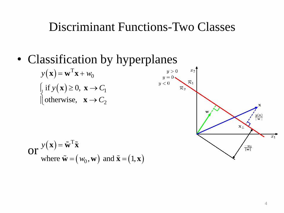
Discriminant Functions-Two Classes

• Classification by hyperplanes

or

4

T0

1

2

if 0,

otherwise,

y w

y C

C

x w x

x x

x

T

0where , and 1,

y

w

x w x

w w x x

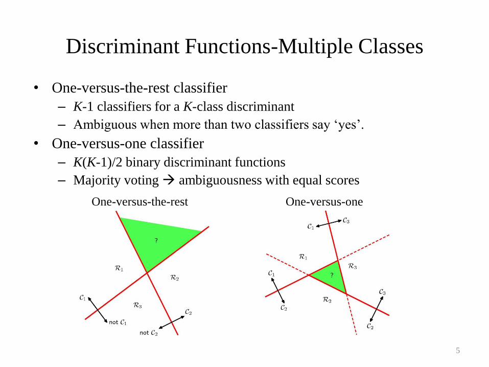
Discriminant Functions-Multiple Classes

• One-versus-the-rest classifier

– K-1 classifiers for a K-class discriminant

– Ambiguous when more than two classifiers say ‘yes’.

• One-versus-one classifier

– K(K-1)/2 binary discriminant functions

– Majority voting ambiguousness with equal scores

5

One-versus-the-rest One-versus-one

Discriminant Functions-Multiple Classes

(Cont’d)

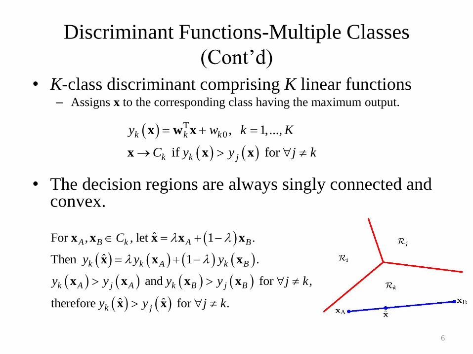
• K-class discriminant comprising K linear functions– Assigns x to the corresponding class having the maximum output.

• The decision regions are always singly connected and convex.

6

T0 , 1,...,

if for

k k k

k k j

y w k K

C y y j k

x w x

x x x

ˆFor , , let 1 .

ˆThen 1 .

and for ,

ˆ ˆtherefore for .

A B k A B

k k A k B

k A j A k B j B

k j

C

y y y

y y y y j k

y y j k

x x x x x

x x x

x x x x

x x

Approaches for Learning Parameters

for Linear Discriminant Functions

• Least square method

• Fisher’s linear discriminant– Relation to least squares

– Multiple classes

• Perceptron algorithm

7

Least Square Method

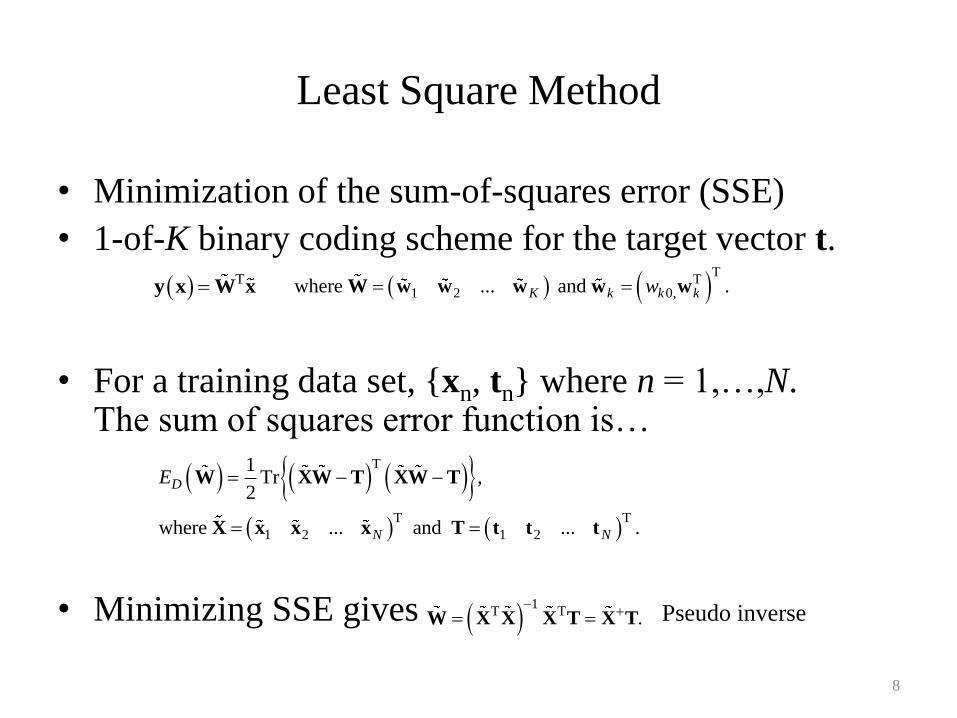
• Minimization of the sum-of-squares error (SSE)

• 1-of-K binary coding scheme for the target vector t.

• For a training data set, {xn, tn} where n = 1,…,N.The sum of squares error function is…

• Minimizing SSE gives

8

Ty x W x T

T1 2 0,where ... and .K k k kw W w w w w w

T

T T

1 2 1 2

1Tr ,

2

where ... and ... .

D

N N

E

W XW T XW T

X x x x T t t t

1

T T .

W X X X T X T Pseudo inverse

Least Square Method (Cont’d)

-Limit and Disadvantage

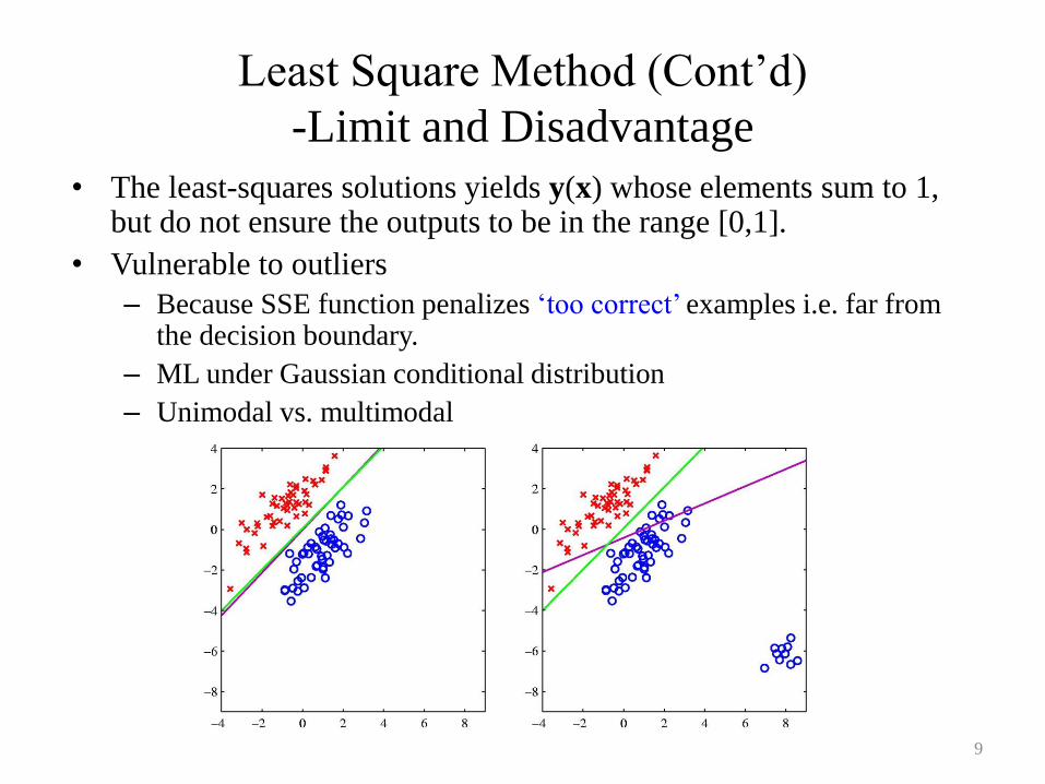
• The least-squares solutions yields y(x) whose elements sum to 1, but do not ensure the outputs to be in the range [0,1].

• Vulnerable to outliers

– Because SSE function penalizes ‘too correct’ examples i.e. far from the decision boundary.

– ML under Gaussian conditional distribution

– Unimodal vs. multimodal

9

Least Square Method (Cont’d)

-Limit and Disadvantage

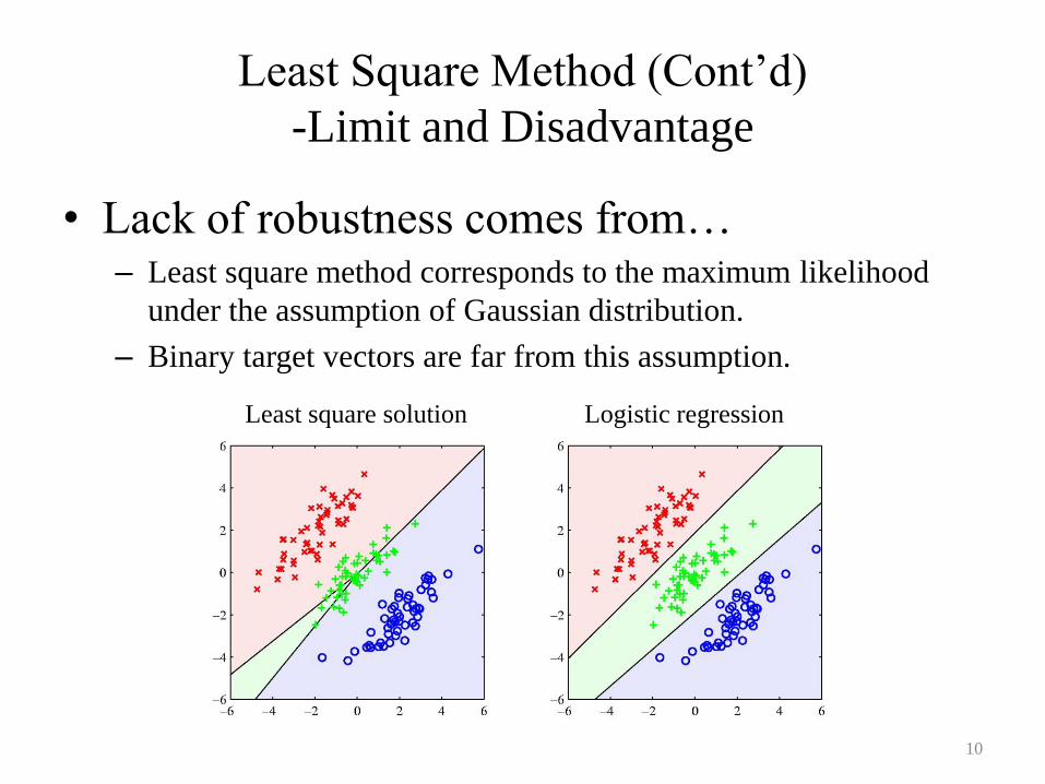
• Lack of robustness comes from…– Least square method corresponds to the maximum likelihood

under the assumption of Gaussian distribution.

– Binary target vectors are far from this assumption.

10

Least square solution Logistic regression

Fisher’s Linear Discriminant

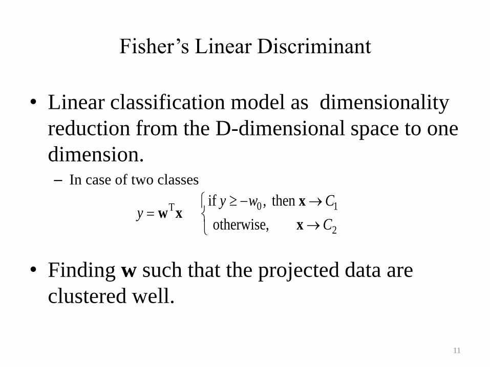
• Linear classification model as dimensionality

reduction from the D-dimensional space to one

dimension.– In case of two classes

• Finding w such that the projected data are

clustered well.

11

Ty w x0 1

2

if , then

otherwise,

y w C

C

x

x

Fisher’s Linear Discriminant (Cont’d)

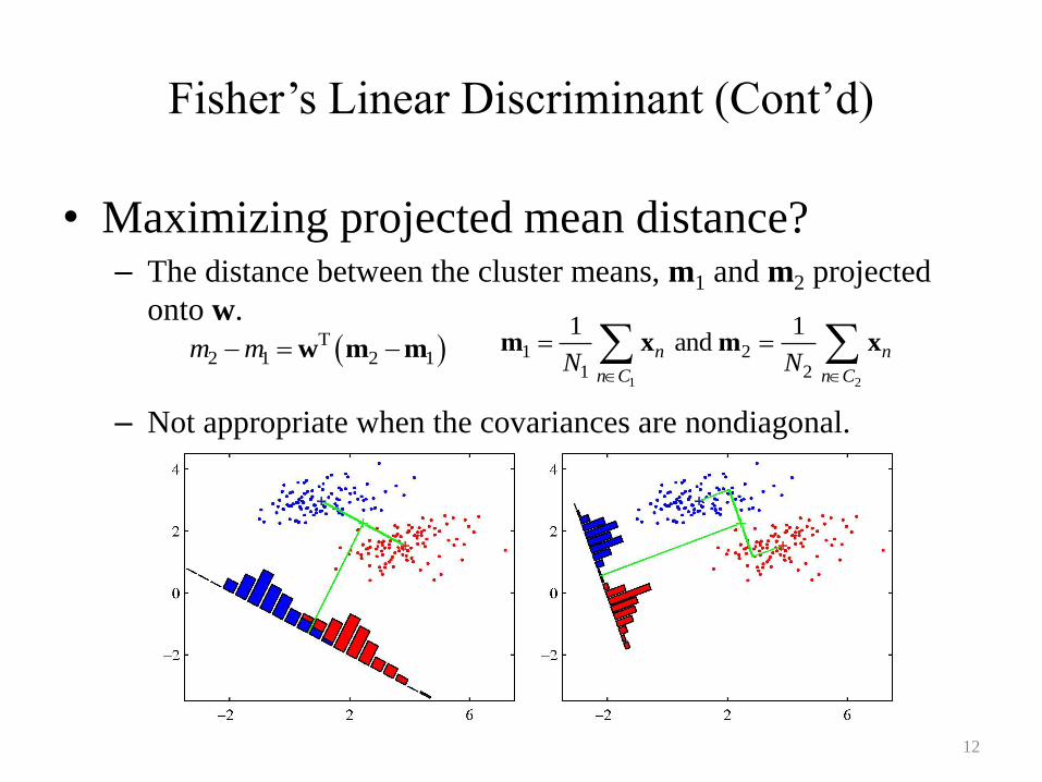
• Maximizing projected mean distance?– The distance between the cluster means, m1 and m2 projected

onto w.

– Not appropriate when the covariances are nondiagonal.

12

1 2

1 21 2

1 1 and n n

n C n CN N

m x m x T2 1 2 1m m w m m

Fisher’s Linear Discriminant (Cont’d)

• Integrate the within-class variance of the projected data.

• Finding w that maximizes J(w).

• J(w) is maximized when

• Fisher’s linear discriminant

• If the within-class covariance is isotropic, w is proportional to the difference of the class means as in the previous case.

13

2

22 1 2

2 22

, where

k

k n k

i n C

m mJ s y m

s s

w

T

TB

W

J w S w

ww S w

1 2

T

2 1 2 1

T T

1 1 2 2

B

W n n n n

n C n C

S m m m m

S x m x m x m x m

SB: Between-class covariance matrix

SW: Within-class covariance matrix

12 1W

w S m m

T TB W W Bw S w S w w S w S w

in the direction

of (m2-m1)

Fisher’s Linear Discriminant

-Relation to Least Squares-

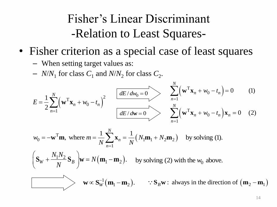
• Fisher criterion as a special case of least squares– When setting target values as:

– N/N1 for class C1 and N/N2 for class C2.

14

2

T0

1

1

2

N

n n

n

E w t

w x

T0

1

T0

1

0 (1)

0 (2)

N

n n

n

N

n n n

n

w t

w t

w x

w x x/ 0dE d w

0/ 0dE dw

by solving (1).

1 21 2 .W B

N NN

N

S S w m m

T0 1 1 2 2

1

1 1, where

N

n

n

w m N NN N

w m x m m

0by solving (2) with the above.w

11 2 .W

w S m m 2 1: always in the direction of B S w m m

Fisher’s Discriminant for Multiple Classes

• K > 2 classes

• Dimension reduction from D to D’– D’ > 1 linear features, yk (k = 1,…,D’)

• Generalization of SW and SB

15

Tk ky w x

T

1 1 1

1 1, where .

.

N N K

T n n n k k

n n k

T W B

NN N

S x m x m m x m

S S S

T

1

T

1

1, where and .

k k

K

W k k n k n k k nkk n C n C

K

B k k k

k

N

N

S S S x m x m m x

S m m m m

SB is from the decomposition of total covariance matrix (Duda and Hart, 1997)

Fisher’s Discriminant for Multiple Classes

(Cont’d)

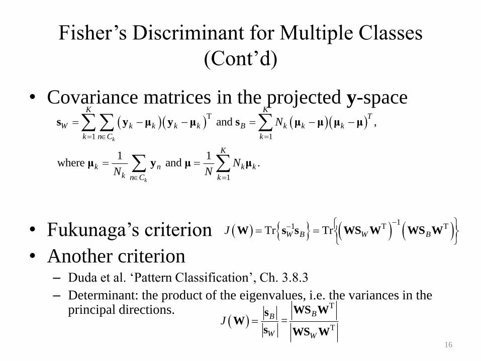
• Covariance matrices in the projected y-space

• Fukunaga’s criterion

• Another criterion– Duda et al. ‘Pattern Classification’, Ch. 3.8.3

– Determinant: the product of the eigenvalues, i.e. the variances in the principal directions.

16

1

1 T TTr TrW B W BJ

W s s WS W WS W

T

1 1

1

and ,

1 1where and .

k

k

K KT

W k k k k B k k k

k n C k

K

k n k kk n C k

N

NN N

s y μ y μ s μ μ μ μ

μ y μ μ

T

T=

BB

W W

J WS Ws

Ws WS W

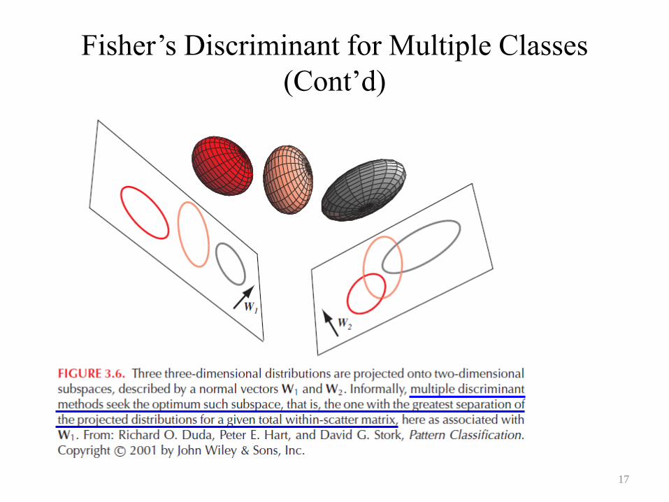
Fisher’s Discriminant for Multiple Classes

(Cont’d)

17

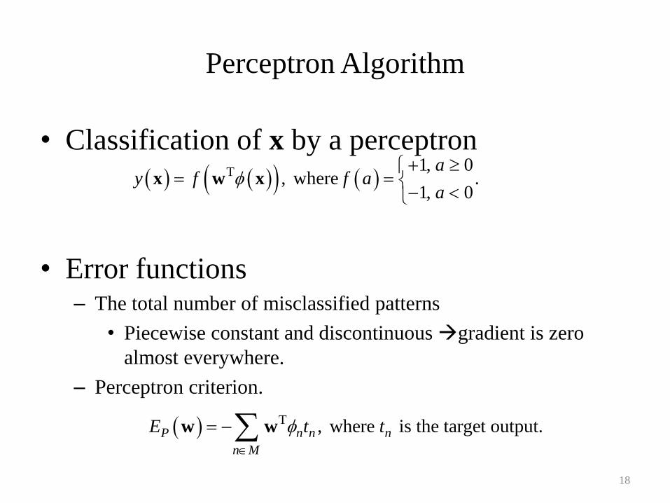
Perceptron Algorithm

• Classification of x by a perceptron

• Error functions– The total number of misclassified patterns

• Piecewise constant and discontinuous gradient is zero

almost everywhere.

– Perceptron criterion.

18

T 1, 0, where .

1, 0

ay f f a

a

x w x

T , where is the target output.P n n n

n M

E t t

w w

Perceptron Algorithm (cont’d)

• Stochastic gradient descent algorithm

• The error from a misclassified pattern is reduced after each iteration.

– Not imply the overall error is reduced.

• Perceptron convergence theorem.

– If there exists an exact solution (i.e. linear separable), the perceptron

learning algorithm is guaranteed to find it.

• However…

– Learning speed, linearly nonseparable, multiple classes

19

1P n nE t

w w w w

T1 T T Tn n n n n n n n n nt t t t t

w w w

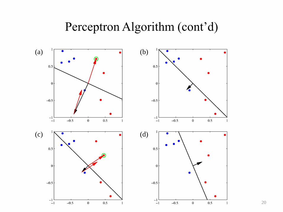
Perceptron Algorithm (cont’d)

20

(a) (b)

(c) (d)

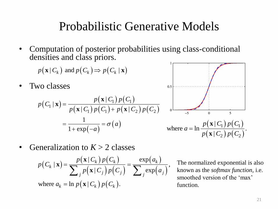
Probabilistic Generative Models

• Computation of posterior probabilities using class-conditional densities and class priors.

• Two classes

• Generalization to K > 2 classes

21

| and |k k kp C p C p Cx x

1 11

1 1 2 2

||

| |

1

1 exp

p C p Cp C

p C p C p C p C

aa

xx

x x

1 1

2 2

|where ln .

|

p C p Ca

p C p C

x

x

| exp| ,

| exp

where ln | .

k k kk

j j jj j

k k k

p C p C ap C

p C p C a

a p C p C

x

xx

x

The normalized exponential is also

known as the softmax function, i.e.

smoothed version of the ‘max’

function.

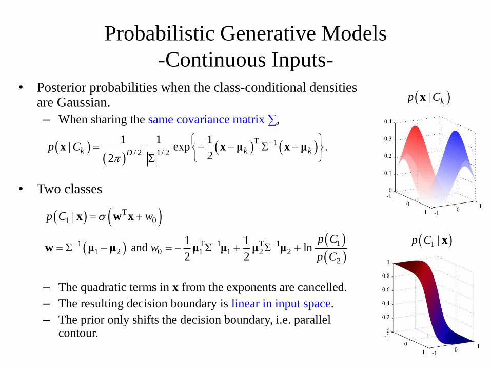
Probabilistic Generative Models

-Continuous Inputs-

• Posterior probabilities when the class-conditional densities are Gaussian.

– When sharing the same covariance matrix ∑,

• Two classes

– The quadratic terms in x from the exponents are cancelled.

– The resulting decision boundary is linear in input space.

– The prior only shifts the decision boundary, i.e. parallel contour.

22

T 1

/ 2 1/ 2

1 1 1| exp .

22k k kD

p C

x x μ x μ

T1 0

11 T 1 T 11 2 0 1 1 2 2

2

|

1 1 and ln

2 2

p C w

p Cw

p C

x w x

w μ μ μ μ μ μ

| kp Cx

1 |p C x

Probabilistic Generative Models

-Continuous Inputs (cont’d)-

• Generalization to K classes

– When sharing the same covariance matrix, the decision boundaries are

linear again.

– If each class-condition density have its own covariance matrix, we will

obtain quadratic functions of x, giving rise to a quadratic discriminant.

23

T0

1 T 10

1 and ln

2

k k k

k k k k k k

a w

w p C

x w x

w μ μ μ

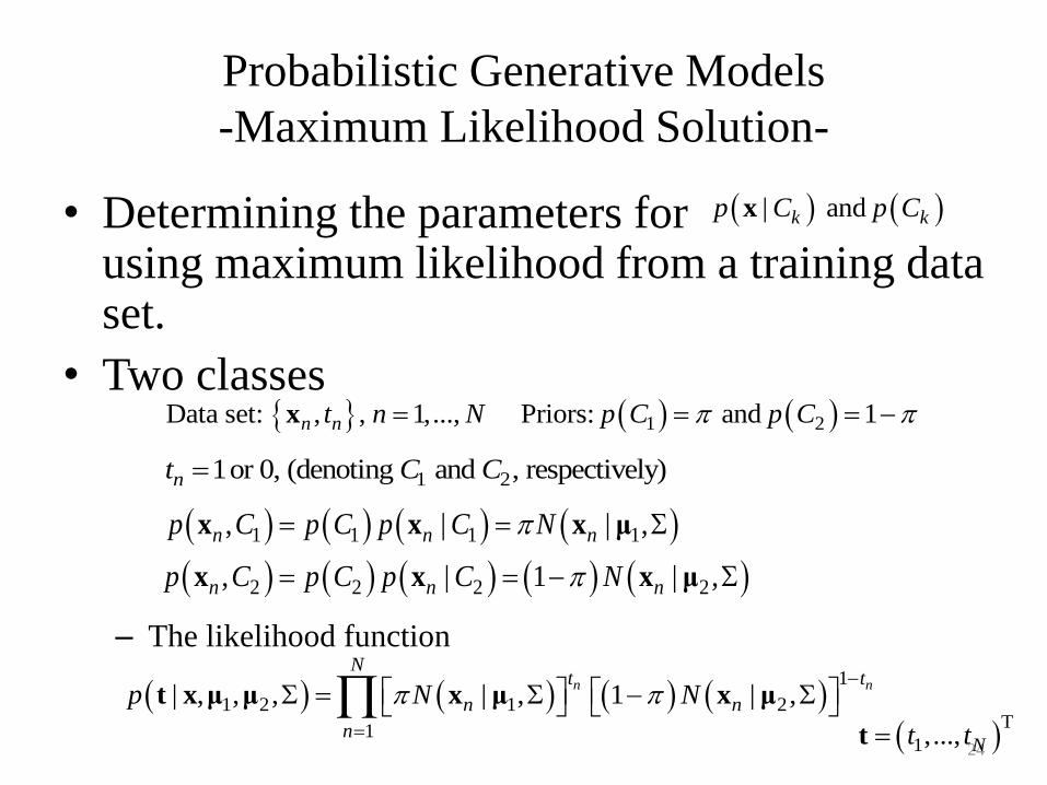
Probabilistic Generative Models

-Maximum Likelihood Solution-

• Determining the parameters for using maximum likelihood from a training data set.

• Two classes

– The likelihood function

24

| and k kp C p Cx

1 1 1 1

2 2 2 2

, | | ,

, | 1 | ,

n n n

n n n

p C p C p C N

p C p C p C N

x x x μ

x x x μ

Data set: , , 1,...,n nt n Nx 1 2Priors: and 1p C p C

1

1 2 1 2

1

| , , , | , 1 | ,n n

Nt t

n n

n

p N N

t x μ μ x μ x μ

1 21or 0, (denoting and , respectively)nt C C

T

1,..., Nt tt

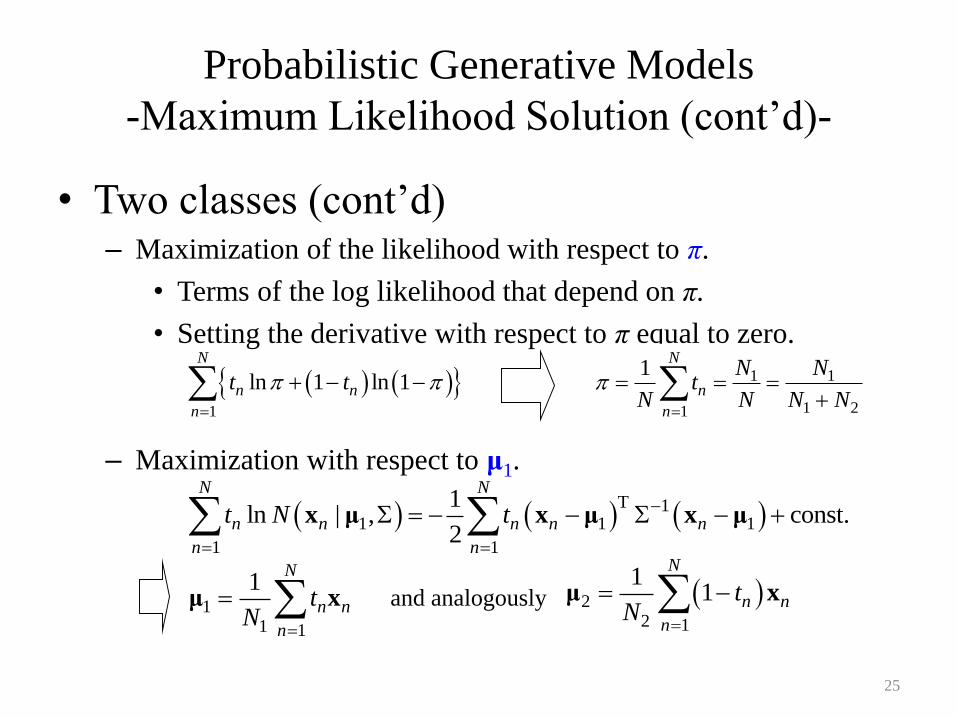
Probabilistic Generative Models

-Maximum Likelihood Solution (cont’d)-

• Two classes (cont’d)– Maximization of the likelihood with respect to π.

• Terms of the log likelihood that depend on π.

• Setting the derivative with respect to π equal to zero.

– Maximization with respect to μ1.

25

1

ln 1 ln 1

N

n n

n

t t

1 1

1 21

1N

n

n

N Nt

N N N N

T 1

1 1 1

1 1

1ln | , const.

2

N N

n n n n n

n n

t N t

x μ x μ x μ

11 1

1N

n n

n

tN

μ x 22 1

11

N

n n

n

tN

μ xand analogously

Probabilistic Generative Models

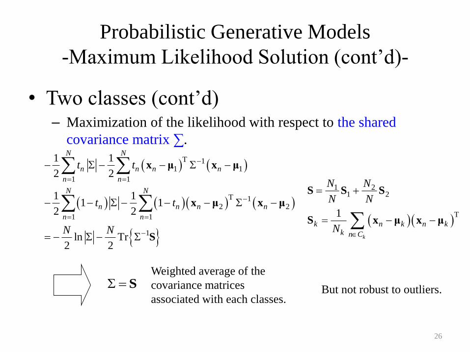
-Maximum Likelihood Solution (cont’d)-

• Two classes (cont’d)– Maximization of the likelihood with respect to the shared

covariance matrix ∑.

26

T 11 1

1 1

T 12 2

1 1

1

1 1

2 2

1 11 1

2 2

ln Tr2 2

N N

n n n n

n n

N N

n n n n

n n

t t

t t

N N

x μ x μ

x μ x μ

S

1 21 2

T1

k

k n k n kk n C

N N

N N

N

S S S

S x μ x μ

SWeighted average of the

covariance matrices

associated with each classes.But not robust to outliers.

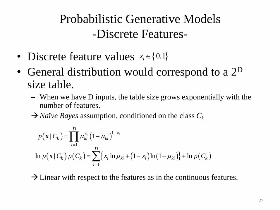
Probabilistic Generative Models

-Discrete Features-

• Discrete feature values

• General distribution would correspond to a 2D

size table.– When we have D inputs, the table size grows exponentially with the

number of features.

Naïve Bayes assumption, conditioned on the class Ck

Linear with respect to the features as in the continuous features.

27

1

1

| 1 ii

Dxx

k kiki

i

p C

x

0,1ix

1

ln | ln 1 ln 1 ln

D

k k i ki i ki k

i

p C p C x x p C

x

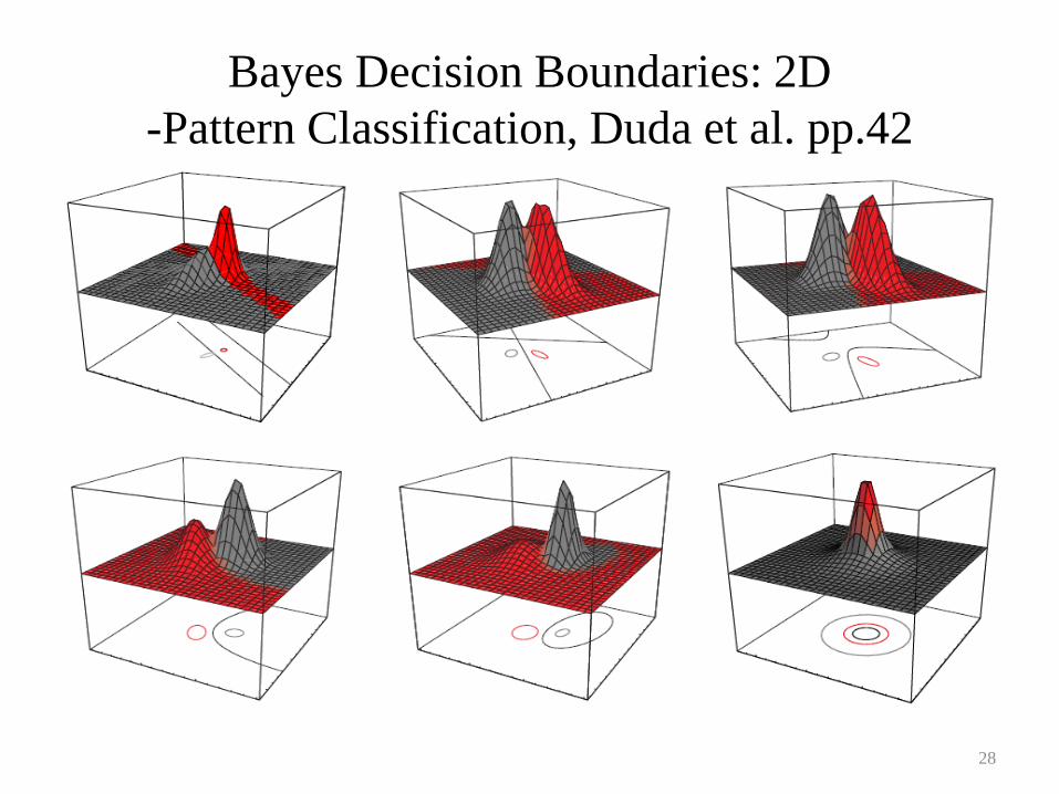
Bayes Decision Boundaries: 2D

-Pattern Classification, Duda et al. pp.42

28

Bayes Decision Boundaries: 3D

-Pattern Classification, Duda et al. pp.43

29

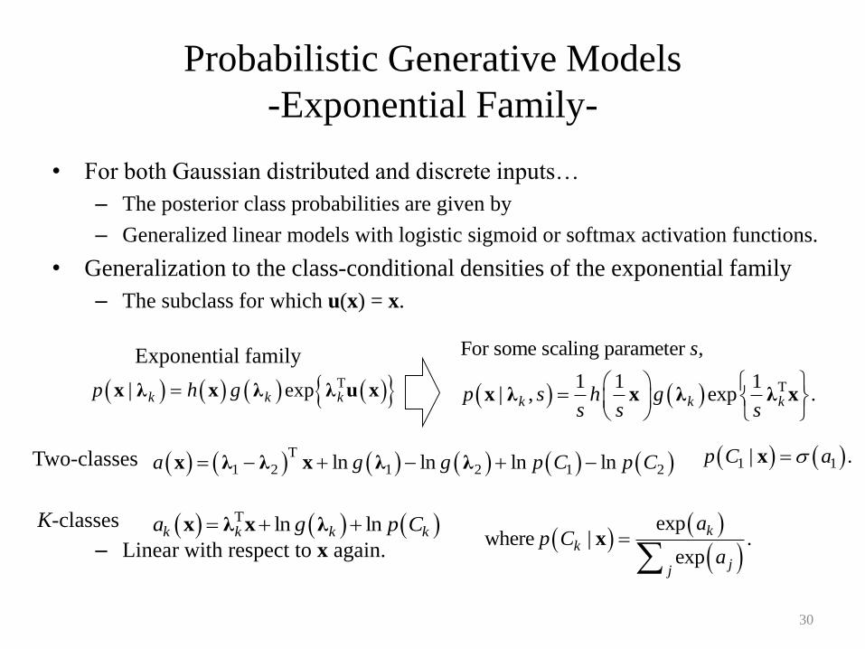
Probabilistic Generative Models

-Exponential Family-

• For both Gaussian distributed and discrete inputs…

– The posterior class probabilities are given by

– Generalized linear models with logistic sigmoid or softmax activation functions.

• Generalization to the class-conditional densities of the exponential family

– The subclass for which u(x) = x.

– Linear with respect to x again.

30

T

For some scaling parameter ,

1 1 1| , exp .k k k

s

p s h gs s s

x λ x λ λ x T| expk k kp h gx λ x λ λ u x

T

1 2 1 2 1 2ln ln ln lna g g p C p C x λ λ x λ λ

Exponential family

T ln lnk k k ka g p C x λ x λ

Two-classes

K-classes

exp

where | .exp

kk

jj

ap C

a

x

1 1| .p C ax

3 Approaches for classification

– Discriminant Functions

– Probabilistic Generative Models

• Fit class-conditional densities and class priors separately

• Apply Bayes’ theorem to find the posterior class probabilities

• Posterior probability of a class can be written as

– Logistic sigmoid acting on a linear function of x (2 classes)

– Softmax transformation of a linear function of x (Multiclass)

• The parameters of the densities as well as the class priors can be

determined using Maximum Likelihood

– Probabilistic Discriminative Models

• Use the functional form of the generalized linear model explicitly

• Determine the parameters directly using Maximum Likelihood

31

Fixed basis functions

• Assume fixed nonlinear transformation

– Transform inputs using a vector of basis functions

– The resulting decision boundaries will be linear in the feature space

32

Logistic regression

• Logistic regression model

– Posterior probability of a class for two-class problem:

• The number of adjustable parameters (M-dimensional, 2-class)

– 2 Gaussian class conditional densities (generative model)

• 2M parameters for means

• M(M+1)/2 parameters for (shared) covariance matrix

• Grows quadratically with M

– Logistic regression (discriminative model)

• M parameters for

• Grows linearly with M

33

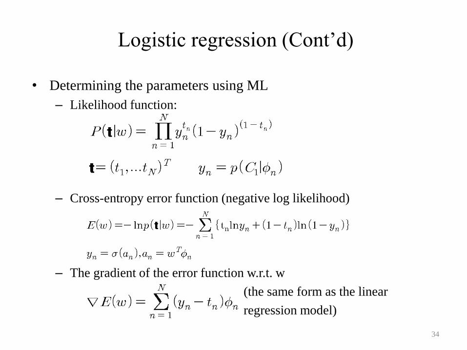
Logistic regression (Cont’d)

• Determining the parameters using ML

– Likelihood function:

– Cross-entropy error function (negative log likelihood)

– The gradient of the error function w.r.t. w

(the same form as the linear

regression model)

34

Iterative reweighted least squares

• Linear regression models in ch.3

– ML solution on the assumption of a Gaussian noise leads to a close-form

solution, as a consequence of the quadratic dependence of the log

likelihood on the parameter w.

• Logistic regression model

– No longer a closed-form solution

– But the error function is concave and has a unique minimum

• Efficient iterative technique can be used

• The Newton-Raphson update to minimize a function E(w)

– Where H is the Hessian matrix, the second derivatives of E(w)

35

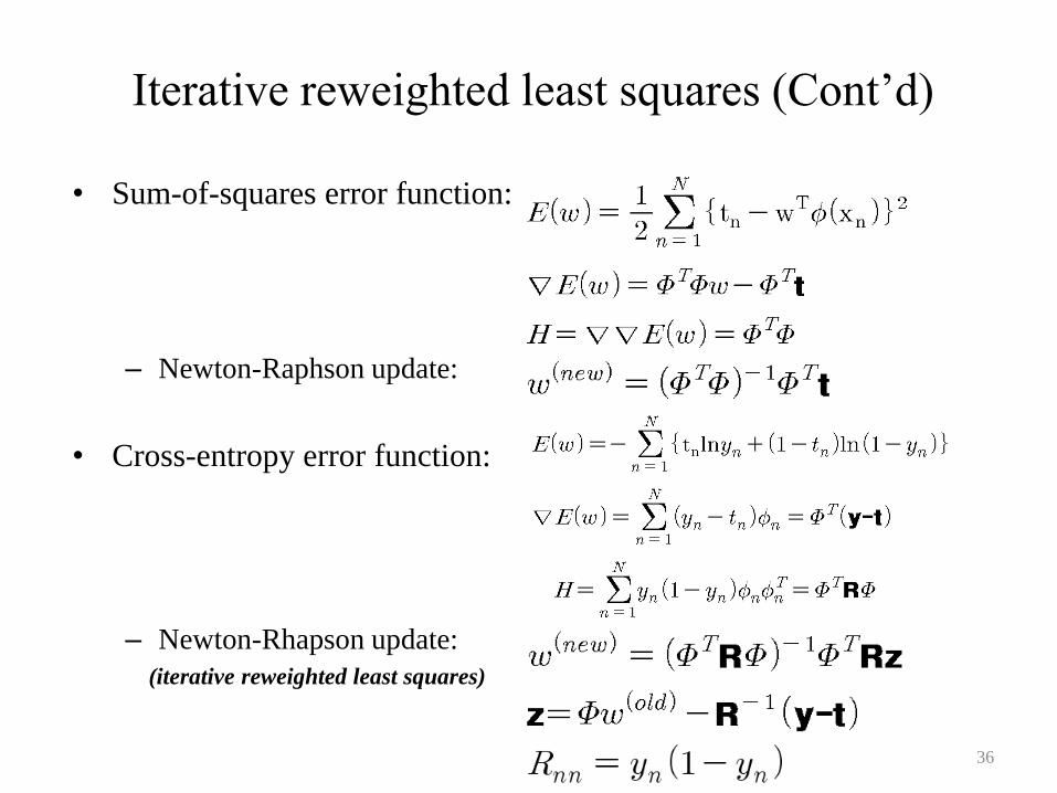
Iterative reweighted least squares (Cont’d)

• Sum-of-squares error function:

– Newton-Raphson update:

• Cross-entropy error function:

– Newton-Rhapson update:

(iterative reweighted least squares)

36

Multiclass logistic regerssion

• Posterior probability for multiclass classification

• We can use ML to determine the parameters directly.

– Likelihood function using 1-of-K coding scheme

– Cross-entropy error function for the multiclass classification

37

Multiclass logistic regression (Cont’d)

• The derivative of the error function

– Same form, the product of error and the basis function.

• The Hessian matrix

– IRLS algorithm can also be used for a batch processing

38

Probit regression

• For a broad range of class-conditional distributions, described by the

exponential family, the resulting posterior class probabilities are

given by a logistic(or softmax) transformation acting on a linear

function of the feature variables.

– However, this is not the case for all choices of class-conditional density

– It might be worth exploring other types of discriminative probabilistic

model

39

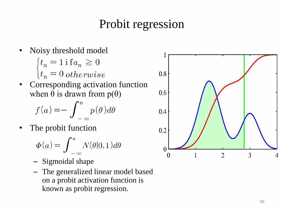
Probit regression

• Noisy threshold model

• Corresponding activation function when θ is drawn from p(θ)

• The probit function

– Sigmoidal shape

– The generalized linear model based on a probit activation function is known as probit regression.

40

Canonical link functions

• We have seen that for some models, if we take the derivative of the error function w.r.t the parameter w, it takes the form of the error times the feature vector.– Logistic regression model with sigmoid activation function

– Logistic regression model with softmax activation function

• This is a general result of assuming a conditional distribution for the target variable from the exponential family, along with a corresponding choice for the activation function known as the canonical link function.

41

Canonical link functions (Cont’d)

• Conditional distributions of the target variable

– Log likelihood:

– The derivative of the log likelihood:

where

• The canonical link function:

then

42

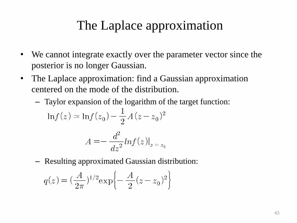
The Laplace approximation

• We cannot integrate exactly over the parameter vector since the

posterior is no longer Gaussian.

• The Laplace approximation: find a Gaussian approximation

centered on the mode of the distribution.

– Taylor expansion of the logarithm of the target function:

– Resulting approximated Gaussian distribution:

43

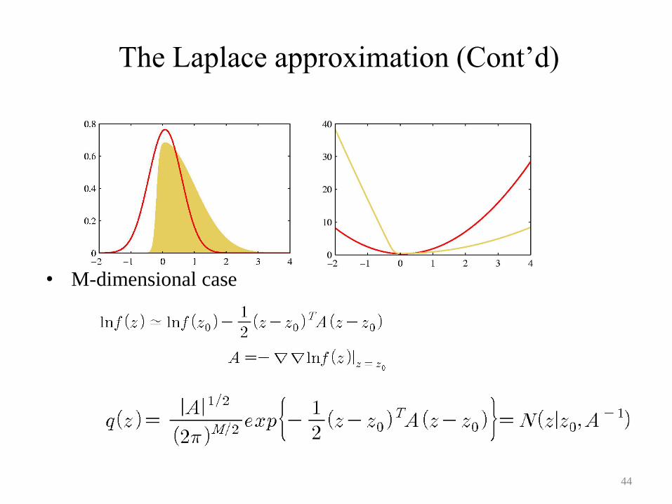
The Laplace approximation (Cont’d)

• M-dimensional case

44

Model comparison and BIC

• Laplace approximation to the normalization constant Z

– This result can be used to obtain an approximation to the model

evidence, which plays a central role in Bayesian model comparison.

• Consider a set of models having parameters

– The log of model evidence can be approximated as

– Further approximation with some more assumption:

Bayesian Information Criterion (BIC)

45

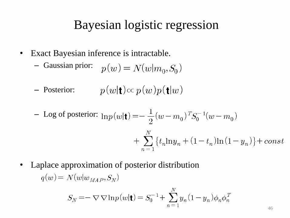
Bayesian logistic regression

• Exact Bayesian inference is intractable.

– Gaussian prior:

– Posterior:

– Log of posterior:

• Laplace approximation of posterior distribution

46

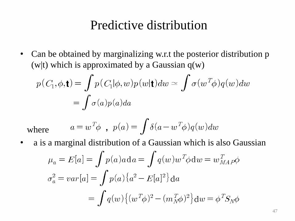
Predictive distribution

• Can be obtained by marginalizing w.r.t the posterior distribution p

(w|t) which is approximated by a Gaussian q(w)

where

• a is a marginal distribution of a Gaussian which is also Gaussian

47

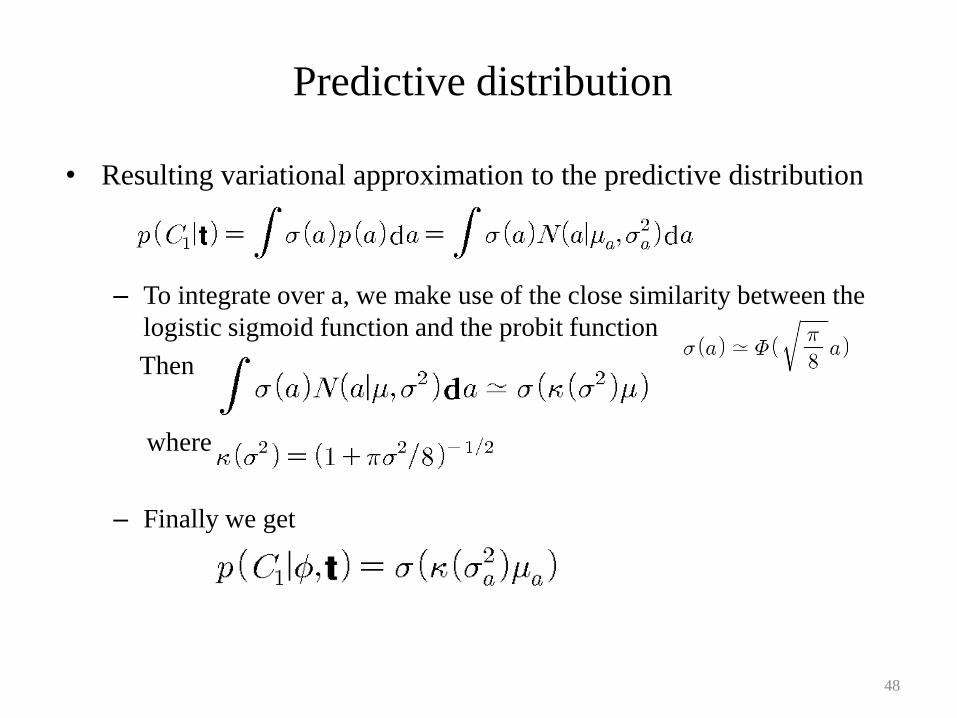
Predictive distribution

• Resulting variational approximation to the predictive distribution

– To integrate over a, we make use of the close similarity between the

logistic sigmoid function and the probit function

Then

where

– Finally we get

48