ch 4. linear models for classification adopted from seung-joon yi biointelligence laboratory, seoul...

Ch 4. Linear Models for Ch 4. Linear Models for ClassificationClassification

Adopted from Seung-Joon YiBiointelligence Laboratory, Seoul National University

http://bi.snu.ac.kr/

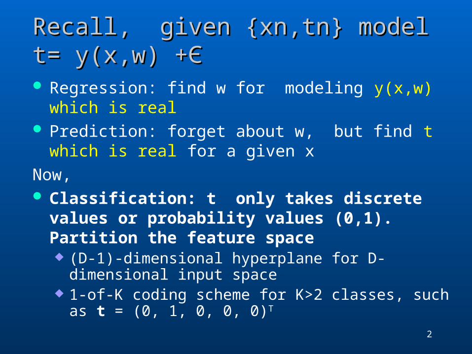
Recall, given {xn,tn} model t= y(x,w) +Recall, given {xn,tn} model t= y(x,w) +ЄЄ

Regression: find w for modeling y(x,w) which is real Prediction: forget about w, but find t which is real for a

given xNow, Classification: t only takes discrete values or probability

values (0,1). Partition the feature space (D-1)-dimensional hyperplane for D-dimensional input

space 1-of-K coding scheme for K>2 classes, such as t = (0, 1, 0, 0,

0)T

2

Need to generalize Need to generalize y(x)=f (wTx + w0) .

Activation function

3(C) 2006, SNU Biointelligence Lab, http://bi.snu.ac.kr/



ContentsContents

Deterministic Models:Discriminant Functions

Find yk(x) to partition the feature space into decision regions

Probabilistic Models Generative Models:

Inference : Model p(x/Ck) and p(Ck) Decision : Model p(Ck/x)

Discriminative Models Model p(Ck/x) directly

|kp C x


Discriminant FunctionDiscriminant Function

A discriminant is a function that takes an input vector x and assigns it to one of K classes, denoted Ck . Linear discriminants,

y(x)=wTx + w0

5

CONCEPT OF SPACECONCEPT OF SPACE

Vector SpacesVector Spaces

Space of vectors, closed under addition and scalar multiplication

Scaler product, dot product, normScaler product, dot product, norm

Norm of ImagesNorm of Images

Orthogonal Images, Distance,BasisOrthogonal Images, Distance,Basis

Cauchy Schwartz InequalityCauchy Schwartz InequalityU+VU+V≤≤UU++VV

Schwartz InequalitySchwartz Inequality


Discriminant Functions-Two ClassesDiscriminant Functions-Two Classes

Classification by hyperplanes

or

T0

1

2

if 0,

otherwise,

y w

y C

C

x w x

x x

x

T

0where , and 1,

y

w

x w x

w w x x



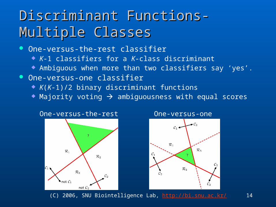
Discriminant Functions-Multiple ClassesDiscriminant Functions-Multiple Classes

One-versus-the-rest classifier K-1 classifiers for a K-class discriminant Ambiguous when more than two classifiers say ‘yes’.

One-versus-one classifier K(K-1)/2 binary discriminant functions Majority voting ambiguousness with equal scores

One-versus-the-rest One-versus-one



Discriminant Functions-Multiple Classes Discriminant Functions-Multiple Classes (Cont’d)(Cont’d) K-class discriminant comprising K linear functions

Assigns x to the corresponding class having the maximum output.

The decision regions are always singly connected and convex.

T0 , 1,...,

if for

k k k

k k j

y w k K

C y y j k

x w x

x x x

ˆFor , , let 1 .

ˆThen 1 .

and for ,

ˆ ˆtherefore for .

A B k A B

k k A k B

k A j A k B j B

k j

C

y y y

y y y y j k

y y j k

x x x x x

x x x

x x x x

x x


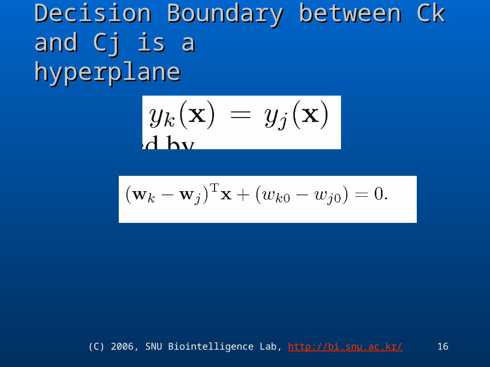
Decision Boundary between Ck and Cj is a Decision Boundary between Ck and Cj is a hyperplanehyperplane




Approaches for Learning ParametersApproaches for Learning Parametersfor Linear Discriminant Functionsfor Linear Discriminant Functions Least square method Fisher’s linear discriminant

Relation to least squares Multiple classes

Perceptron algorithm



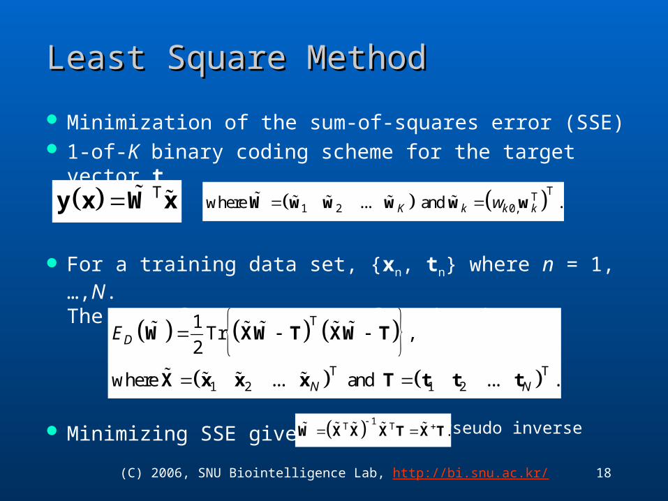
Least Square MethodLeast Square Method

Minimization of the sum-of-squares error (SSE) 1-of-K binary coding scheme for the target vector t.

For a training data set, {xn, tn} where n = 1,…,N.The sum of squares error function is…

Minimizing SSE gives

Ty x W x TT1 2 0,where ... and .K k k kw W w w w w w

T

T T1 2 1 2

1Tr ,

2

where ... and ... .

D

N N

E

W XW T XW T

X x x x T t t t

1T T . W X X X T X T Pseudo inverse



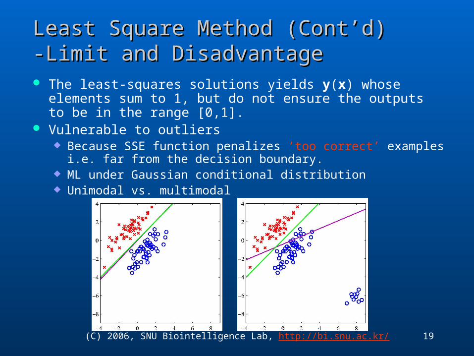
Least Square Method (Cont’d)Least Square Method (Cont’d)-Limit and Disadvantage-Limit and Disadvantage The least-squares solutions yields y(x) whose elements sum to 1,

but do not ensure the outputs to be in the range [0,1]. Vulnerable to outliers

Because SSE function penalizes ‘too correct’ examples i.e. far from the decision boundary.

ML under Gaussian conditional distribution Unimodal vs. multimodal



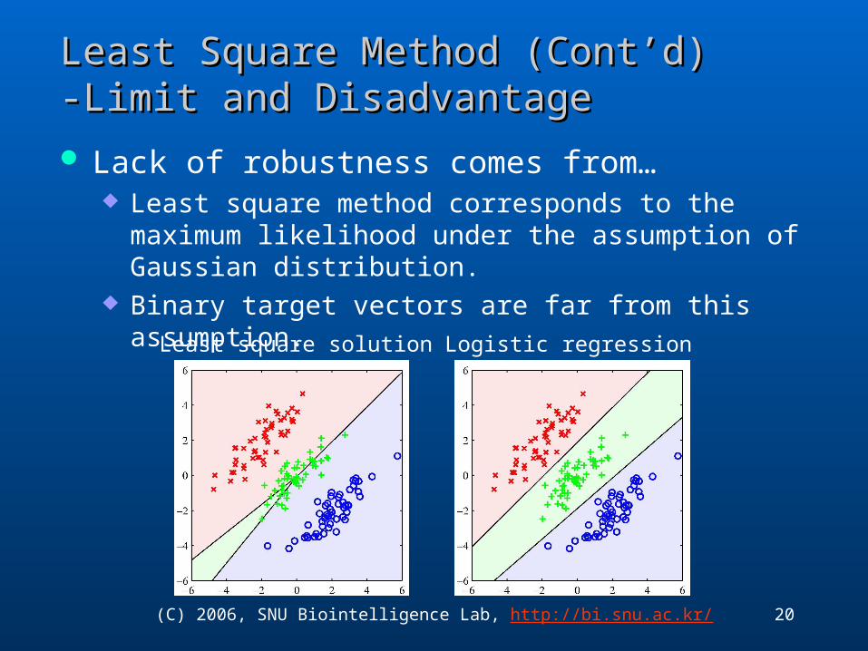
Least Square Method (Cont’d)Least Square Method (Cont’d)-Limit and Disadvantage-Limit and Disadvantage Lack of robustness comes from…

Least square method corresponds to the maximum likelihood under the assumption of Gaussian distribution.

Binary target vectors are far from this assumption.

Least square solution Logistic regression



Fisher’s Linear DiscriminantFisher’s Linear Discriminant

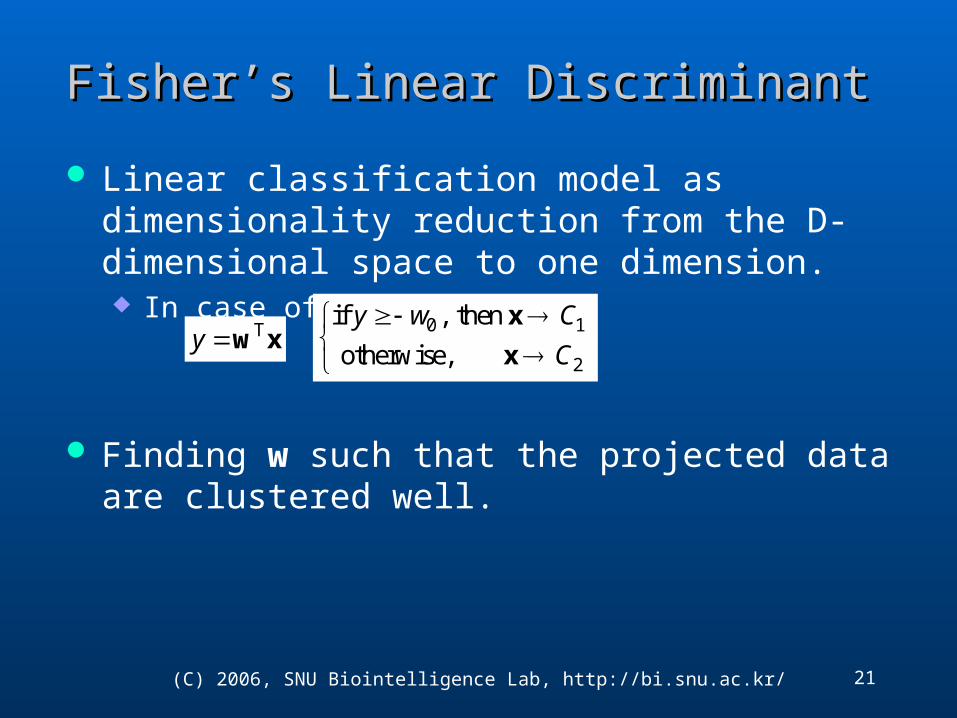
Linear classification model as dimensionality reduction from the D-dimensional space to one dimension. In case of two classes

Finding w such that the projected data are clustered well.

Ty w x0 1

2

if , then

otherwise,

y w C

C

x

x


Fisher’s Linear Discriminant (Cont’d)Fisher’s Linear Discriminant (Cont’d)

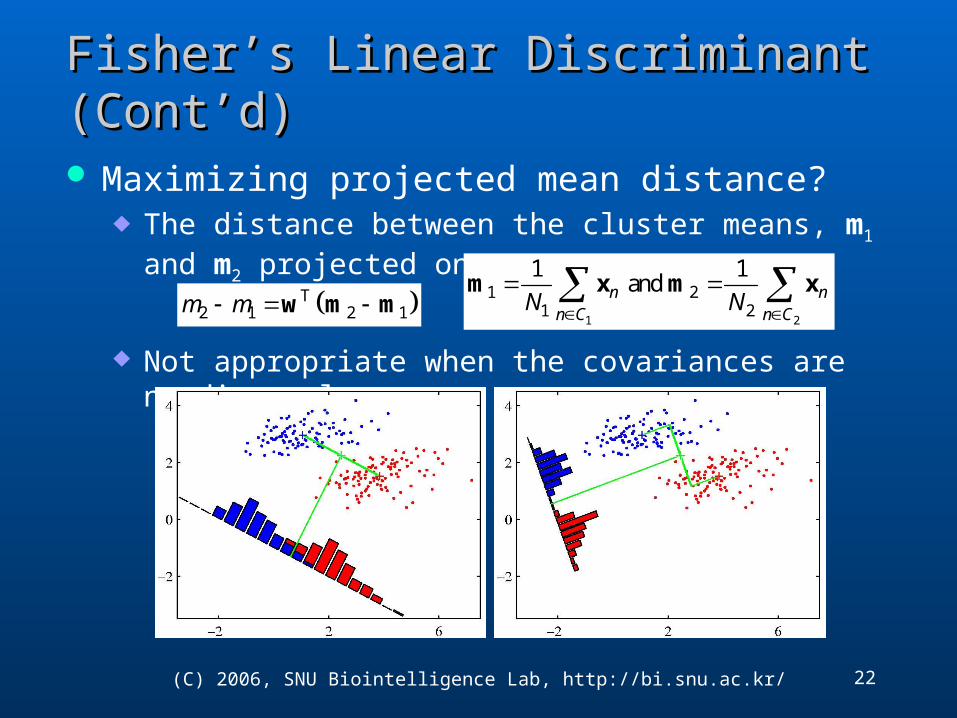
Maximizing projected mean distance? The distance between the cluster means, m1 and m2 projected

onto w.

Not appropriate when the covariances are nondiagonal.1 2

1 21 2

1 1 and n n

n C n CN N

m x m x T

2 1 2 1m m w m m


Fisher’s Linear Discriminant (Cont’d)Fisher’s Linear Discriminant (Cont’d)

Integrate the within-class variance of the projected data. Finding w that maximizes J(w).

J(w) is maximized when

Fisher’s linear discriminant If the within-class covariance is isotropic, w is proportional to the

difference of the class means as in the previous case.

2

22 1 22 2

2

, where k

k n ki n C

m mJ s y m

s s

w

T

TB

W

J w S w

ww S w

1 2

T2 1 2 1

T T1 1 2 2

B

W n n n nn C n C

S m m m m

S x m x m x m x m

SB: Between-class covariance matrix

SW: Within-class covariance matrix

12 1W

w S m m

T TB W W Bw S w S w w S w S w in the direction

of (m2-m1)


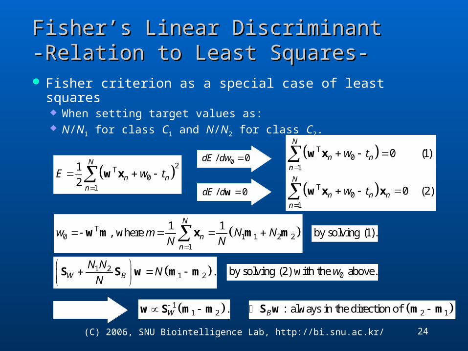
Fisher’s Linear DiscriminantFisher’s Linear Discriminant-Relation to Least Squares--Relation to Least Squares- Fisher criterion as a special case of least squares

When setting target values as: N/N1 for class C1 and N/N2 for class C2.

2T0

1

1

2

N

n nn

E w t

w x

T0

1

T0

1

0 (1)

0 (2)

N

n nn

N

n n nn

w t

w t

w x

w x x/ 0dE d w

0/ 0dE dw

by solving (1).

1 21 2 .W B

N NN

N S S w m m

T0 1 1 2 2

1

1 1, where

N

nn

w m N NN N

w m x m m

0by solving (2) with the above.w

11 2 .W

w S m m 2 1: always in the direction of B S w m m


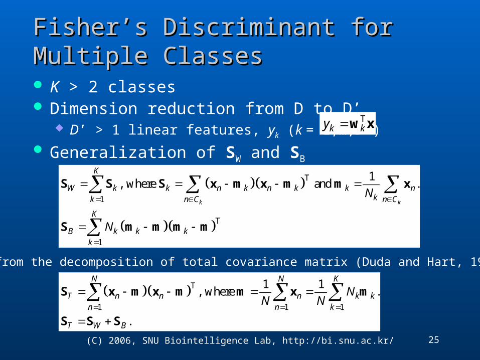
Fisher’s Discriminant for Multiple ClassesFisher’s Discriminant for Multiple Classes

K > 2 classes Dimension reduction from D to D’

D’ > 1 linear features, yk (k = 1,…,D’) Generalization of SW and SB

Tk ky w x

T

1 1 1

1 1, where .

.

N N K

T n n n k kn n k

T W B

NN N

S x m x m m x m

S S S

T

1

T

1

1, where and .

k k

K

W k k n k n k k nkk n C n C

K

B k k kk

N

N

S S S x m x m m x

S m m m m

SB is from the decomposition of total covariance matrix (Duda and Hart, 1997)


Fisher’s Discriminant for Multiple Classes Fisher’s Discriminant for Multiple Classes (Cont’d)(Cont’d) Covariance matrices in the projected y-space

Fukunaga’s criterion Another criterion

Duda et al. ‘Pattern Classification’, Ch. 3.8.3 Determinant: the product of the eigenvalues, i.e. the variances

in the principal directions.

11 T TTr TrW B W BJ

W s s WS W WS W

T

1 1

1

and ,

1 1where and .

k

k

K KT

W k k k k B k k kk n C k

K

k n k kk n C k

N

NN N

s y μ y μ s μ μ μ μ

μ y μ μ

T

T=

BB

W W

J WS Ws

Ws WS W


Fisher’s Discriminant for Multiple Classes Fisher’s Discriminant for Multiple Classes (Cont’d)(Cont’d)

Perceptron:F. RosenblattPerceptron:F. Rosenblatt

Connectionism: Birth of ANN: Kohonen, Hopefield, Inspired from Biological Neurons

28

=f(wTx)

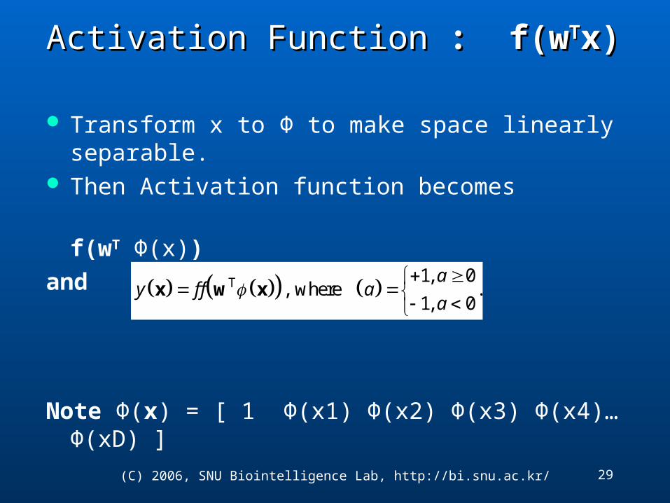
Activation Function Activation Function : f(w: f(wTTx)x)

Transform x to Φ to make space linearly separable. Then Activation function becomes f(wT Φ(x))and

Note Φ(x) = [ 1 Φ(x1) Φ(x2) Φ(x3) Φ(x4)… Φ(xD) ]


T 1, 0, where .

1, 0

ay f f a

a

x w x

Goal: Find wGoal: Find w

Define a cost function and minimiz it w.r. To w We want f(wT Φ(x)) tn≥ 0Recall , t {-1, +1} ∈



Perceptron CriterionPerceptron Criterion

Let M is the set of misclassified samples by w

T , where is the target output.P n n nn M

E t t

w w

32

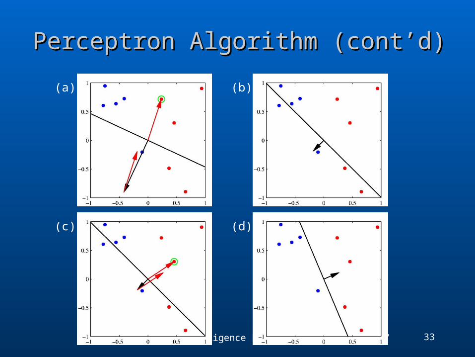
Stochastic gradient descent algorithmStochastic gradient descent algorithm

The error from a misclassified pattern is reduced after each iteration. Not imply the overall error is reduced.

Perceptron convergence theorem. If there exists an exact solution (i.e. linear separable), the perceptron

learning algorithm is guaranteed to find it.

1P n nE t w w w w

T1 T T Tn n n n n n n n n nt t t t t w w w


Perceptron Algorithm (cont’d)Perceptron Algorithm (cont’d)

(a) (b)

(c) (d)

Problems with PerceptromProblems with Perceptrom

Learning speed, Poor results for linearly nonseparable, Difficult to apply to multiple classes İt is deterministic

34

35

Probabilistic Approaches for ClassificationProbabilistic Approaches for Classification Generative Models

Inference: Model class-conditional densities and class priors

Decision: Apply Bayes’ theorem to find the posterior class probabilities.

Probabilistic Discriminative Models Use the functional form of the generalized linear model explicitly Determine the parameters directly using Maximum Likelihood

Comes from population growth Prob distribution function of Norlam R.V. İs Logistic sigmoid İf class conditional densities are Normal, posteriors become

logistic sigmoid

Logistic Sigmoid FunctionLogistic Sigmoid Function

36

simple[2] logistic function may be defined by the formula

Posterior Probabilities can be formulated Posterior Probabilities can be formulated by by 2-Class: Logistic sigmoid acting on a linear function

of x K-Class: Softmax transformation of a linear function

of x

Then, The parameters of the densities as well as the class

priors can be determined using Maximum Likelihood

37

38

Probabilistic Generative ModelsProbabilistic Generative Models: 2-Class: 2-Class Recall, given

Posterior can be expresses by Logistic Sigmoid

a is called logit function

| and |k k kp C p C p Cx x

1 11

1 1 2 2

||

| |

1

1 exp

p C p Cp C

p C p C p C p C

aa

xx

x x

1 1

2 2

|where ln .

|

p C p Ca

p C p C

x

x

Posterior can be expresses by Softmax function or normalized exponential

Probabilistic Generative Models K-ClassProbabilistic Generative Models K-Class

39

| exp| ,

| exp

where ln | .

k k kk

j j jj j

k k k

p C p C ap C

p C p C a

a p C p C

x

xx

x


Probabilistic Generative ModelsProbabilistic Generative ModelsGaussian Class Conditionals for 2-ClassGaussian Class Conditionals for 2-Class

Assume same covariance matrix ∑,

Note The quadratic terms in x from the exponents are cancelled. The resulting decision boundary is linear in input space. The prior only shifts the decision boundary, i.e. parallel

contour.

T 1/ 2 1/ 2

1 1 1| exp .

22k k kD

p C

x x μ x μ

T1 0

11 T 1 T 11 2 0 1 1 2 2

2

|

1 1 and ln

2 2

p C w

p Cw

p C

x w x

w μ μ μ μ μ μ

| kp Cx

1 |p C x


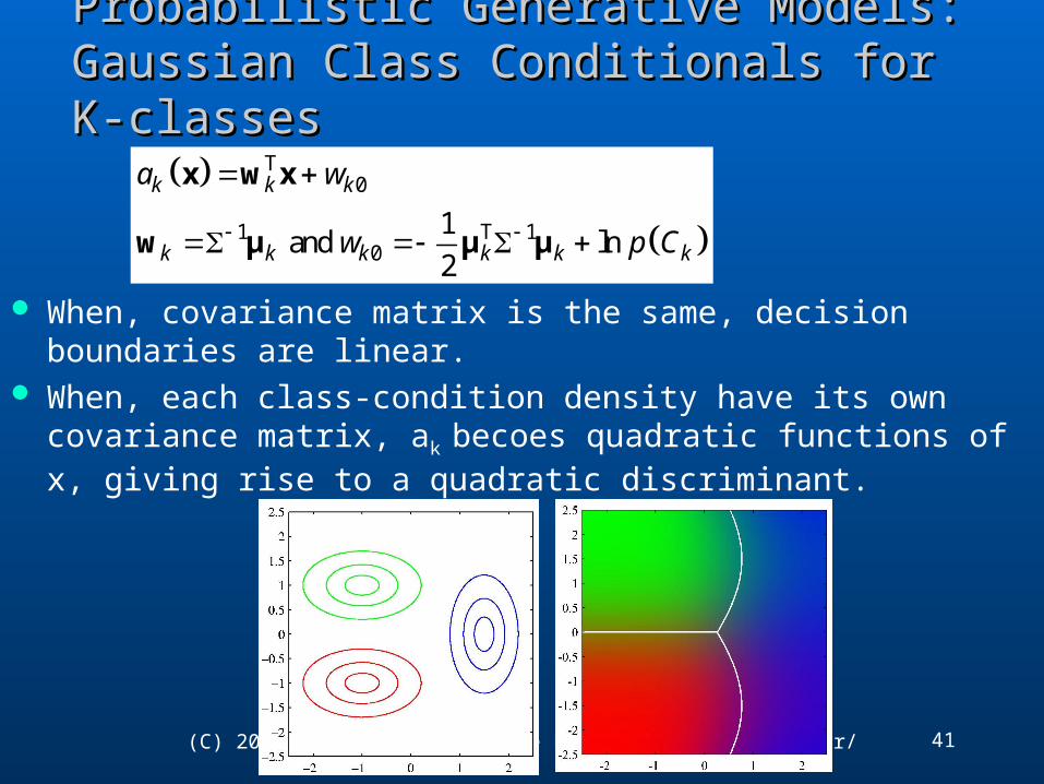
Probabilistic Generative ModelsProbabilistic Generative Models: Gaussian Class : Gaussian Class Conditionals for K-classesConditionals for K-classes

When, covariance matrix is the same, decision boundaries are linear. When, each class-condition density have its own covariance matrix,

ak becoes quadratic functions of x, giving rise to a quadratic discriminant.

T0

1 T 10

1 and ln

2

k k k

k k k k k k

a w

w p C

x w x

w μ μ μ


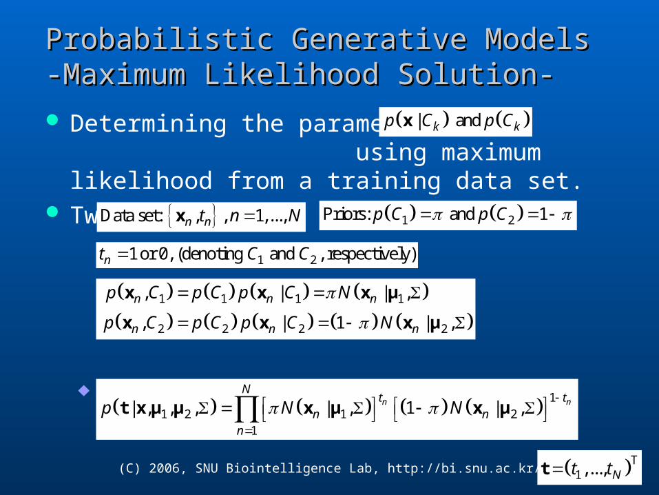
Probabilistic Generative ModelsProbabilistic Generative Models-Maximum Likelihood Solution--Maximum Likelihood Solution- Determining the parameters for using

maximum likelihood from a training data set. Two classes

The likelihood function

| and k kp C p Cx

1 1 1 1

2 2 2 2

, | | ,

, | 1 | ,

n n n

n n n

p C p C p C N

p C p C p C N

x x x μ

x x x μ

Data set: , , 1,...,n nt n Nx 1 2Priors: and 1p C p C

11 2 1 2

1

| , , , | , 1 | ,n nN

t tn n

n

p N N

t x μ μ x μ x μ

1 21 or 0, (denoting and , respectively)nt C C

T1,..., Nt tt

Q: Find the parameters of p(Ck/x)Q: Find the parameters of p(Ck/x)

P(Ck) μ1, μ2 and


Probabilistic Generative ModelsProbabilistic Generative Models-Maximum Likelihood Solution-Maximum Likelihood Solution

Let P(C1) = π and P(C2) = 1- π

44

45

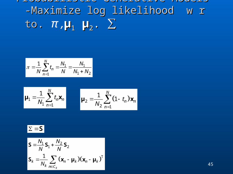
Probabilistic Generative ModelsProbabilistic Generative Models-Maxim-Maximize log likelihood w r toize log likelihood w r to. . π ,μμ11 μ μ22. ∑. ∑

.

1 1

1 21

1 N

nn

N Nt

N N N N

11 1

1 N

n nn

tN

μ x 22 1

11

N

n nn

tN

μ x

1 21 2

T1

k

k n k n kk n C

N N

N N

N

S S S

S x μ x μ

S


Probabilistic Generative ModelsProbabilistic Generative Models-Discrete Features--Discrete Features- Discrete feature values General distribution would correspond to a 2D size table.

When we have D inputs, the table size grows exponentially with the number of features.

Naïve Bayes assumption, conditioned on the class Ck

Linear with respect to the features as in the continuous features.

11

| 1 ii

Dxx

k kikii

p C

x

0,1ix

1

ln | ln 1 ln 1 lnD

k k i ki i ki ki

p C p C x x p C

x


Bayes Decision Boundaries: 2DBayes Decision Boundaries: 2D-Pattern Classification, Duda et al. pp.42-Pattern Classification, Duda et al. pp.42


Bayes Decision Boundaries: 3DBayes Decision Boundaries: 3D-Pattern Classification, Duda et al. pp.43-Pattern Classification, Duda et al. pp.43


Probabilistic Generative ModelsProbabilistic Generative Models-Exponential Family--Exponential Family- For both Gaussian distributed and discrete inputs…

The posterior class probabilities are given by Generalized linear models with logistic sigmoid or softmax activation

functions. Generalization to the class-conditional densities of the exponential family

The subclass for which u(x) = x.

Linear with respect to x again.

T

For some scaling parameter ,

1 1 1| , exp .k k k

s

p s h gs s s

x λ x λ λ x T| expk k kp h gx λ x λ λ u x

T1 2 1 2 1 2ln ln ln lna g g p C p C x λ λ x λ λ

Exponential family

T ln lnk k k ka g p C x λ x λ

Two-classes

K-classes

exp

where | .exp

kk

jj

ap C

a

x

1 1| .p C ax

Probabilistic Discriminative ModelsProbabilistic Discriminative Models

Goal: Find p(Ck/x) directly Discriminative Training: Max likelihood p(Ck/x) İmroves prediction performance when p(x/Ck) is poorly

estimated



Fixed basis functionsFixed basis functions: x : x

Assume fixed nonlinear transformation Transform inputs using a vector of basis functions The resulting decision boundaries will be linear in the feature

space y(x)= WT Φ


Logistic Logistic RRegressionegression Model Model

Posterior probability of a class for two-class problem:

The number of adjustable parameters (M-dimensional, 2-class) 2 Gaussian class conditional densities (generative model)

2M parameters for means M(M+1)/2 parameters for (shared) covariance matrix Grows quadratically with M

Logistic regression (discriminative model) M parameters for Grows linearly with M


Logistic Logistic RRegression (Cont’d)egression (Cont’d)

Determining the parameters using ML Likelihood function:

Cross-entropy error function (negative log likelihood) the cross entropy between two probability distributions measures the

average number of bits needed to identify an event from a set of possibilities, if a coding scheme is used based on a given probability distribution q, rather than the "true" distribution p.

The gradient of the error function w.r.t. WThe gradient of the error function w.r.t. W

The same form as the linear regression regression model)



Iterative Iterative RReweighted eweighted LLeast east SSquaresquares

Linear regression models in ch.3 ML solution on the assumption of a Gaussian noise leads to a close-

form solution, as a consequence of the quadratic dependence of the log likelihood on the parameter w.

Logistic regression model No longer a closed-form solution But the error function is concave and has a unique minimum

Efficient iterative technique can be used The Newton-Raphson update to minimize a function E(w)

– Where H is the Hessian matrix, the second derivatives of E(w)


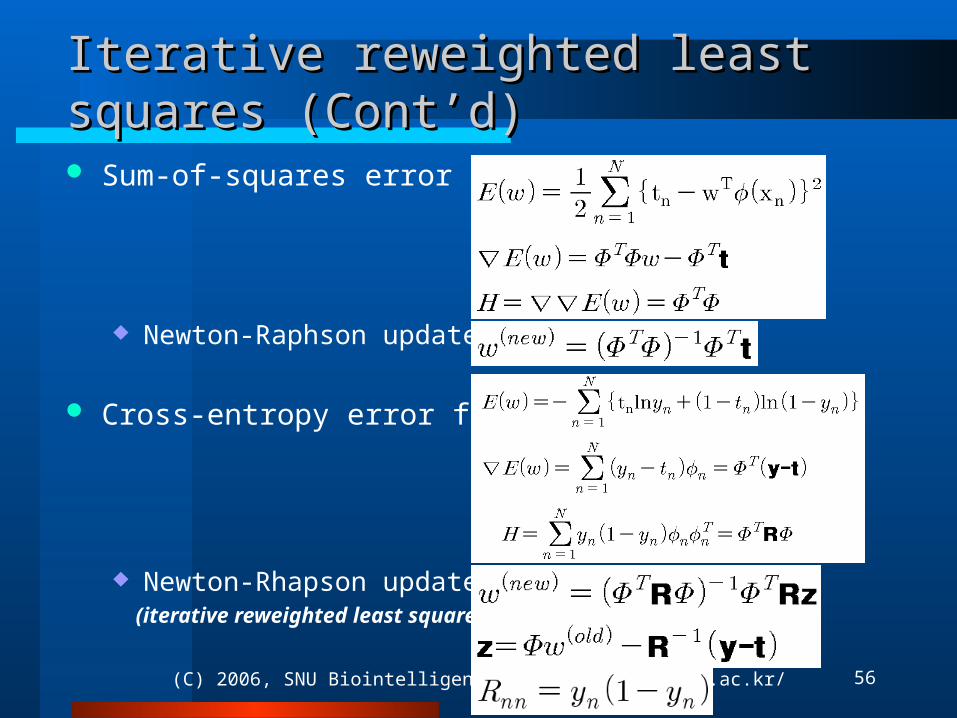
Iterative reweighted least squares (Cont’d)Iterative reweighted least squares (Cont’d)

Sum-of-squares error function:

Newton-Raphson update:

Cross-entropy error function:

Newton-Rhapson update: (iterative reweighted least squares)


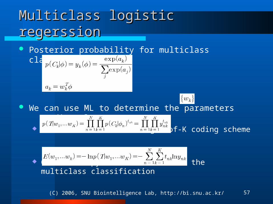
Multiclass logistic regerssionMulticlass logistic regerssion

Posterior probability for multiclass classification

We can use ML to determine the parameters directly. Likelihood function using 1-of-K coding scheme

Cross-entropy error function for the multiclass classification


Multiclass logistic regression (Cont’d)Multiclass logistic regression (Cont’d)

The derivative of the error function

Same form, the product of error times the basis function.

The Hessian matrix

IRLS algorithm can also be used for a batch processing


Probit regressionProbit regression

For a broad range of class-conditional distributions, described by the exponential family, the resulting posterior class probabilities are given by a logistic(or softmax) transformation acting on a linear function of the feature variables.

However this is not the case for all choices of class-conditional density It might be worth exploring other types of discriminative probabilistic

model


Probit regressionProbit regression

Noisy threshold model

Corresponding activation function when θ is drawn from p(θ)

The probit function

Sigmoidal shape The generalized linear model based

on a probit activation function is known as probit regression.

61

Canonical link functionsCanonical link functions

We have seen that for some models, if we take the derivative of the error function w.r.t the parameter w, it takes the form of the error times the feature vector. Logistic regression model with sigmoid activation function

Logistic regression model with softmax activation function

This is a general result of assuming a conditional distribution for the target variable from the exponential family, along with a corresponding choice for the activation function known as the canonical link function.


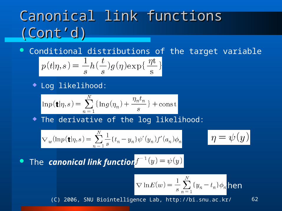
Canonical link functions (Cont’d)Canonical link functions (Cont’d)

Conditional distributions of the target variable

Log likelihood:

The derivative of the log likelihood: where

The canonical link function:

then


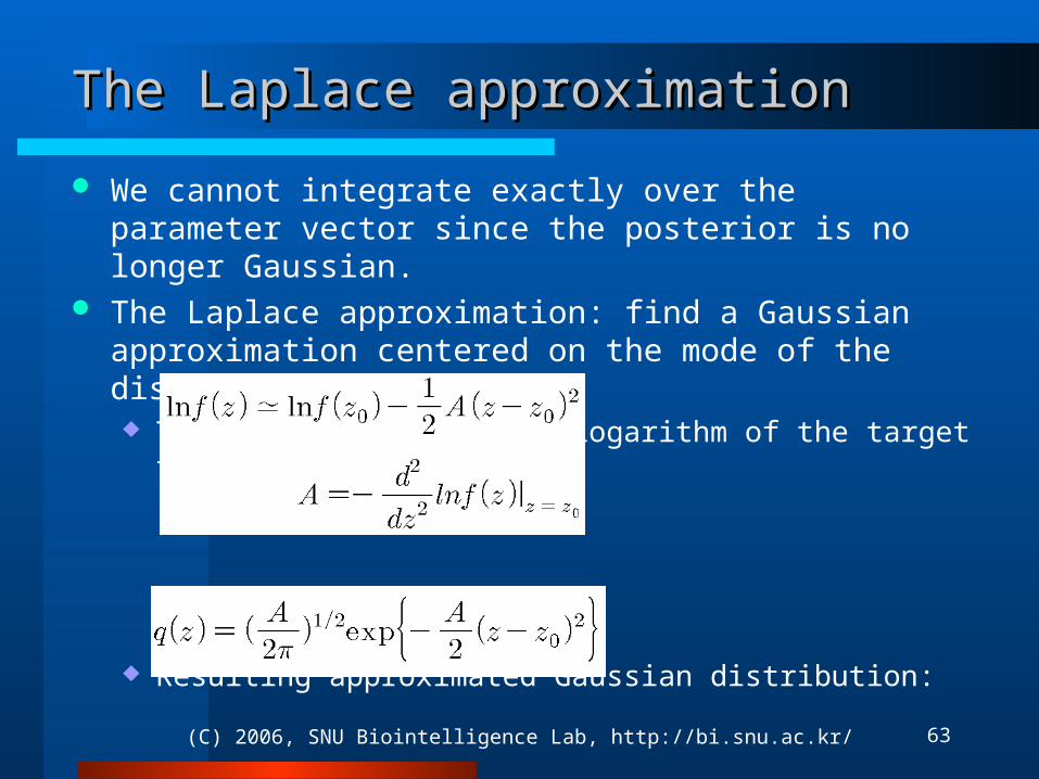
The Laplace approximationThe Laplace approximation

We cannot integrate exactly over the parameter vector since the posterior is no longer Gaussian.

The Laplace approximation: find a Gaussian approximation centered on the mode of the distribution. Taylor expansion of the logarithm of the target function:

Resulting approximated Gaussian distribution:


The Laplace approximation (Cont’d)The Laplace approximation (Cont’d)

M-dimensional case


Model comparison and BICModel comparison and BIC

Laplace approximation to the normalization constant Z

This result can be used to obtain an approximation to the model evidence, which plays a central role in Bayesian model comparison.

Consider a set of models having parameters The log of model evidence can be approximated as

Further approximation with some more assumption: Bayesian Information Criterion (BIC)


Bayesian Logistic RegressionBayesian Logistic Regression

Exact Bayesian inference is intractable. Gaussian prior:

Posterior:

Log of posterior:

Laplace approximation of posterior distribution


Predictive distributionPredictive distribution

Can be obtained by marginalizing w.r.t the posterior distribution p (w|t) which is approximated by a Gaussian q(w)

where a is a marginal distribution of a Gaussian which is also Gaussian


Predictive distributionPredictive distribution

Resulting variational approximation to the predictive distribution

To integrate over a, we make use of the close similarity between the logistic sigmoid function and the probit function

Then

where

Finally we get

ch 4. linear models for classification adopted from seung-joon yi biointelligence laboratory, seoul...

Documents