ch. 4 steady flow in pipes - seoul national university

Seoul National University

Ch. 4 Steady Flow in Pipes4-1 Fundamentals


Ch. 9 Flow in PipesSteady flow9.1 Fundamental equations9.2 Laminar flow9.3 Turbulent flow – Smooth pipes9.4 Turbulent flow – Rough pipes9.5 Classification of smoothness and roughness9.6 Pipe friction factors9.7 Pipe friction in noncircular pipes9.8 Pipe fiction – Empirical formulation9.9 Local losses in pipelines9.10 Pipeline problems – Single pipes9.11 Pipeline problems – Multiple pipes

Unsteady flow9.12 Unsteady flow and water hammer in pipelines9.13 Rigid water column theory9.14 Elastic theory

2

Ch. 4-1

Ch. 6

Ch. 4-3

Ch. 4-2

Ch. 5-1Ch. 5-2


3

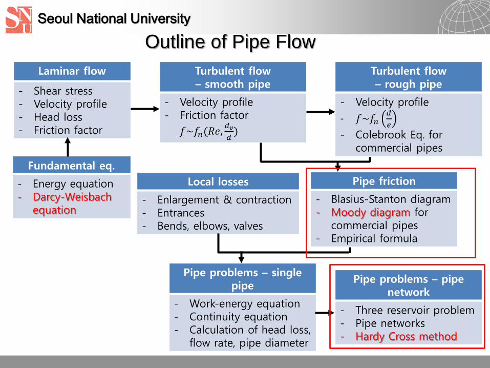
Laminar flow

- Shear stress- Velocity profile- Head loss- Friction factor

Turbulent flow – smooth pipe

- Velocity profile- Friction factor

𝑓𝑓~𝑓𝑓𝑛𝑛(𝑅𝑅𝑅𝑅, 𝑑𝑑𝑣𝑣𝑑𝑑

)

Pipe friction

- Blasius-Stanton diagram- Moody diagram for

commercial pipes- Empirical formula

Local losses

- Enlargement & contraction- Entrances- Bends, elbows, valves

Pipe problems – single pipe

- Work-energy equation- Continuity equation- Calculation of head loss,

flow rate, pipe diameter

Pipe problems – pipe network

- Three reservoir problem- Pipe networks- Hardy Cross method

Fundamental eq.

- Energy equation- Darcy-Weisbach

equation

Turbulent flow – rough pipe

- Velocity profile

- 𝑓𝑓~𝑓𝑓𝑛𝑛𝑑𝑑𝑒𝑒

- Colebrook Eq. for commercial pipes

Outline of Pipe Flow


Contents

4.0 Applications

4.1 Fundamentals Equations

4.2 Laminar Flow


Today’s objectives

Review the shear stress and head loss Understand laminar flows and friction relating problems.

5


4.0 Applications

3D-GIS for pipe-networking

6


City pipe network

Water supply pipe network

7


Diffuser system Wastewater discharge from STP Heated water discharge from power plants Cooled water discharge from LNG terminals Brine discharge from desalination plants

8


Heated water discharge from power plants

9


Heated water diffuser

10


Cooled water diffuser

11


Tampa Bay RO plant (US)

12


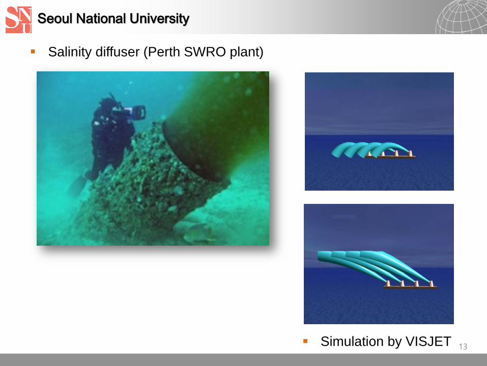
Salinity diffuser (Perth SWRO plant)

13 Simulation by VISJET


4.1 Fundamentals Equations

Newton’s 2nd law of motion → Momentum eq.

In a pipe flow (Ch. 7; p. 260), apply momentum eq.

– where P is wetted perimeter

14

Pressureforce

Shearforce

Gravitationalforce

hh

A AP RR P

⇔= =

( ) ( )out inF Q v Q vρ ρ= −∑ ∑ ∑


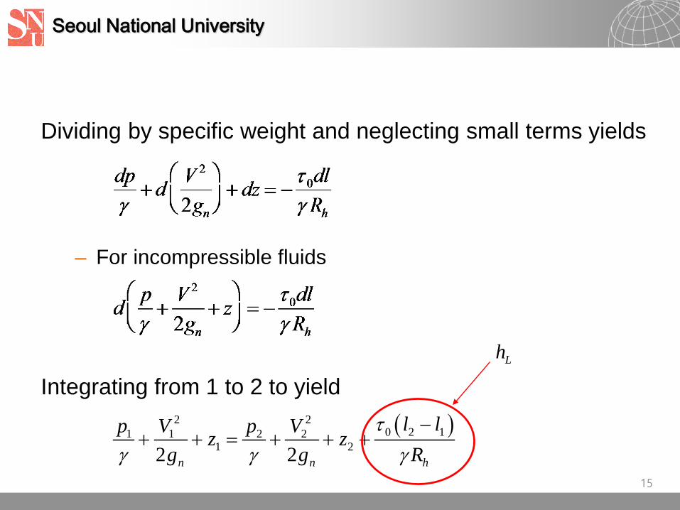
Dividing by specific weight and neglecting small terms yields

– For incompressible fluids

Integrating from 1 to 2 to yield

15

( )2 20 2 11 1 2 2

1 22 2n n h

p pz zl lV V

g Rgτ

γ γ γ+ +

−++= +

Lh


The drop in the energy line is called head loss.

In incompressible flow

For pipe flow,

16

1 2

2 21 1 2 2

1 22 2 Ln n

p pzg g

hV zVγ γ −

+ + = + + +

( )1 2

0 2 1 0L

h h

l lh

Rl

Rτ τ

γ γ−

−= =

1 2 1 20 2

L h Lh R h Rl l

γ γτ − −== =

2

2 2hA R

RRR

Pππ

= = =

(1)

(2)


Work-energy equation

Energy correction factor can be ignored– In turbulent flow (~1), in the most engineering problem– In laminar flow, when energy correction factor is large,

the velocity heads are usually negligible– In most case, anyway, velocity head is very small

compared to other terms

17

(9.1)


Dimensional analysis

Find head loss equation for pipe flowIn smooth pipe, problem parameters are

– Head loss, hL

– Pipe length, l– Pipe diameter, d– Density, ρ– Viscosity, µ– Gravity, g– Velocity, V

18

( ), , , , , , 0Lf h d l V gρ µ =


1. V, d, and ρ do not combine, choose as a repeating variable; k=3 2. In this case, n=7, n-k=4

19

( )

( )

03

02 2

0 01 1

1

0 02

2

2

3

: , , ,

: ,

1, 1

, ,

2, 1, 0, 1

a d

a d

cb

cb

L M MM L t f V d Lt L Lt

L M LM L t f V d g Lt L t

Vda b c d

Va b c dgd

ρ µ

ρ

π

ρπµ

π

π

= =

= =

= = = = − → =

= = − = =

→

=

−

( ) ( )( ) ( )

2 2

3 3 4

1 1

4

, , , ; , , ,

, , , ; , , , L

f V d f V d g

f V d l f V d h

π π

π

µ

π

ρ ρ

ρ ρ

= =

= =

Apply Buckingham Π theory (Ch. 8)


20

2

, ,Lh l Vd d gd

Vdf ρµ

=

( ) ( )

( ) ( )

03 3 3

3

04

0 0

0 01 3

4

0, , 0

0, , 0,

: , , ,

: , , ,

cb

c

ad

ad

Lb

L

L MM L t f V d l L Lt L

L MM L t f V d h L Lt L

la b d cd

ha b d cd

π

π

π

π

ρ

ρ

= =

= =

= = − = → =

=

= − = → =

2 2'

2 2Ll V l Vhd

Vdg

f fd g

ρµ

= =

' Vdf f ρ

µ

=


From experiments, using a dimensionless coefficient of proportionality, f called the friction factor, Darcy, Weisbach and others proposed (Darcy-Weisbach equation) in long straight, uniform pipes

From momentum equation,

Two equations can be combined (D=2R, Rh=πR2/2πR)

21

2

2Ll Vfd

hg

=

(9.3)

(9.2)


In the previous fundamental equation relating wall shear to friction factor, density and mean velocity, it is apparent that f isdimensionless.

Then must have the dimension of velocity. Friction (shear) velocity is defined as

Then we have

22

0* 8

V fv τρ=≡

*

8Vv f=

(9.4)


I.P.

Water flows in a 150mm diameter pipeline at a mean velocity of 4.5m/s. The head lost in 30 m of this pipe is measured experimentally and found to be 5.33 m. Calculate the friction velocity in the pipe.

~ 5.8% of mean velocity

23

2

2Ll Vfd

hg

=


4.2 Laminar Flow Assumptions for the laminar flow in pipe

– Symmetric distribution of shear stress and velocity– Maximum velocity at the center of the pipe and no velocity at

the wall (no-slip condition)– Linear shear stress distribution

24


For laminar flow, combine Eq. 2 and Newton’s viscosity equation

Integrating once w.r.t. r yields

25


Apply the no-slip boundary condition at r=R,

Then,

At the center of pipe

Then

26

20 R

2τ0=- +cμR

( )2 20τv= R2μR

-r

20

cτv = ( 0)2μR

R when r =

2

c 2

rv=v 1-R

Paraboloid → Hagen-Poiseuille flow

(A)

(9.5)


Apply the friction velocity into (A)

When y is small (near the wall), 2nd term is negligible, then velocity profile has a linear relationship with distance from the wall.

27

( ) ( )

( )

22 2 2 2* *

*

222*

*

v vvv = -r = -rv

vv y= y- = R-y )v

R R2νR 2νR

(where rν 2R

→

* 0v = τ /ρ

*

*

vv ν

v y≈

2=kinematic viscosity(m /s)µνρ

=

(9.7)


From Eq. A

We can get flow rate

Since

28

( ) ( )3R R 2 20 0

0 0

R-rπτ πτQ= v 2πrdr = R rdr=μ4μR∫ ∫

L0

γhτ R=2l

42L L

L

4

2L

2

π γh πd γhQ= = , Q=AV=πR8μl μl

γR h γ

R V128

V=8

d h=μl 32μl

( )2 20τv= R2μR

-r


(9.9)

For laminar flow, head loss varies with the first power of the velocity.(Fig. 7.3 of p. 232)

These facts of laminar flow were established experimentally by Hagen (1839) and Poiseuille (1840). → Hagen-Poiseuille law

29

L 2

32μlVhγd

=


Equating the Darcy-Weisbach equation for head loss to Eq. 9.9 yields an expression for the friction factor

(9.10)

In laminar flow, friction factor only depends on the Reynolds number.

30

2

2Ll Vfd

hg

=

2

32L

lVhdµγ

=

ch. 4 steady flow in pipes - seoul national university

Documents