ch07 solns 4e - people.clarkson.edupeople.clarkson.edu/~drasmuss/es 260 fall 2014 exam #2...
TRANSCRIPT
Excerpts from this work may be reproduced by instructors for distribution on a not-for-profit basis for testing or instructional purposes only to students enrolled in courses for which the textbook has been adopted. Any other reproduction or translation of this work beyond that permitted by Sections 107 or 108 of the 1976 United States Copyright Act without the permission of the copyright owner is unlawful.
CHAPTER 7
MECHANICAL PROPERTIES
PROBLEM SOLUTIONS
Concepts of Stress and Strain
7.1 Using mechanics-of-materials principles (i.e., equations of mechanical equilibrium applied to a free-
body diagram), derive Equations 7.4a and 7.4b.
Solution
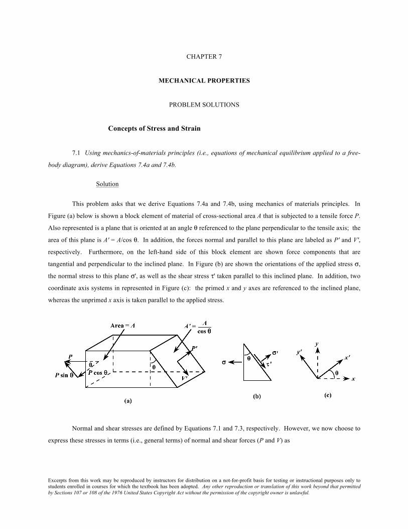
This problem asks that we derive Equations 7.4a and 7.4b, using mechanics of materials principles. In
Figure (a) below is shown a block element of material of cross-sectional area A that is subjected to a tensile force P.
Also represented is a plane that is oriented at an angle θ referenced to the plane perpendicular to the tensile axis; the
area of this plane is A' = A/cos θ. In addition, the forces normal and parallel to this plane are labeled as P' and V',
respectively. Furthermore, on the left-hand side of this block element are shown force components that are
tangential and perpendicular to the inclined plane. In Figure (b) are shown the orientations of the applied stress σ,
the normal stress to this plane σ', as well as the shear stress τ' taken parallel to this inclined plane. In addition, two
coordinate axis systems in represented in Figure (c): the primed x and y axes are referenced to the inclined plane,
whereas the unprimed x axis is taken parallel to the applied stress.
Normal and shear stresses are defined by Equations 7.1 and 7.3, respectively. However, we now choose to
express these stresses in terms (i.e., general terms) of normal and shear forces (P and V) as

Excerpts from this work may be reproduced by instructors for distribution on a not-for-profit basis for testing or instructional purposes only to students enrolled in courses for which the textbook has been adopted. Any other reproduction or translation of this work beyond that permitted by Sections 107 or 108 of the 1976 United States Copyright Act without the permission of the copyright owner is unlawful.
! = PA
! = VA
For static equilibrium in the x' direction the following condition must be met:
F! x'= 0
which means that
P' ! P cos " = 0
Or that
P' = P cos !
Now it is possible to write an expression for the stress
!' in terms of P' and A' using the above expression and the
relationship between A and A' [Figure (a)]:
!' = P’A’
= P cos!A
cos!
= PA
cos2!
However, it is the case that P/A = σ; and, after making this substitution into the above expression, we have Equation
7.4a—that is
! ' = ! cos2"
Now, for static equilibrium in the y' direction, it is necessary that
Fy'! = 0

Excerpts from this work may be reproduced by instructors for distribution on a not-for-profit basis for testing or instructional purposes only to students enrolled in courses for which the textbook has been adopted. Any other reproduction or translation of this work beyond that permitted by Sections 107 or 108 of the 1976 United States Copyright Act without the permission of the copyright owner is unlawful.
= !V' + Psin"
Or
V' = P sin!
We now write an expression for τ' as
!' = V'
A'
And substitution of the above equation for V' and also the expression for A' gives
!' = V'
A'
= P sin!A
cos!
= PA
sin! cos!
= ! sin" cos"
which is just Equation 7.4b.

Excerpts from this work may be reproduced by instructors for distribution on a not-for-profit basis for testing or instructional purposes only to students enrolled in courses for which the textbook has been adopted. Any other reproduction or translation of this work beyond that permitted by Sections 107 or 108 of the 1976 United States Copyright Act without the permission of the copyright owner is unlawful.
7.2 (a) Equations 7.4a and 7.4b are expressions for normal (σ′) and shear (τ′) stresses, respectively, as a
function of the applied tensile stress (σ) and the inclination angle of the plane on which these stresses are taken (θ of
Figure 7.4). Make a plot showing the orientation parameters of these expressions (i.e., cos2 θ and sin θ cos θ)
versus θ.
(b) From this plot, at what angle of inclination is the normal stress a maximum?
(c) At what inclination angle is the shear stress a maximum?
Solution
(a) Below are plotted curves of cos2θ (for
!' ) and sin θ cos θ (for τ') versus θ.
(b) The maximum normal stress occurs at an inclination angle of 0°.
(c) The maximum shear stress occurs at an inclination angle of 45°.

Excerpts from this work may be reproduced by instructors for distribution on a not-for-profit basis for testing or instructional purposes only to students enrolled in courses for which the textbook has been adopted. Any other reproduction or translation of this work beyond that permitted by Sections 107 or 108 of the 1976 United States Copyright Act without the permission of the copyright owner is unlawful.
Stress-Strain Behavior
7.3 A specimen of aluminum having a rectangular cross section 10 mm × 12.7 mm (0.4 in. × 0.5 in.) is
pulled in tension with 35,500 N (8000 lbf) force, producing only elastic deformation. Calculate the resulting strain.
Solution
This problem calls for us to calculate the elastic strain that results for an aluminum specimen stressed in
tension. The cross-sectional area is just (10 mm) × (12.7 mm) = 127 mm2 (= 1.27 × 10⁻⁴ m2 = 0.20 in.2); also, the
elastic modulus for Al is given in Table 7.1 as 69 GPa (or 69 × 109 N/m2). Combining Equations 7.1 and 7.5 and
solving for the strain yields
! = "E
= FA0E
= 35,500 N(1.27 # 10$4 m2)(69 # 109 N/m2) = 4.1 # 10-3

Excerpts from this work may be reproduced by instructors for distribution on a not-for-profit basis for testing or instructional purposes only to students enrolled in courses for which the textbook has been adopted. Any other reproduction or translation of this work beyond that permitted by Sections 107 or 108 of the 1976 United States Copyright Act without the permission of the copyright owner is unlawful.
7.4 A cylindrical specimen of a titanium alloy having an elastic modulus of 107 GPa (15.5 × 10⁶ psi) and
an original diameter of 3.8 mm (0.15 in.) will experience only elastic deformation when a tensile load of 2000 N
(450 lbf) is applied. Compute the maximum length of the specimen before deformation if the maximum allowable
elongation is 0.42 mm (0.0165 in.).
Solution
We are asked to compute the maximum length of a cylindrical titanium alloy specimen (before
deformation) that is deformed elastically in tension. For a cylindrical specimen
A0 = !d02
"
# $
%
& ' 2
where d0 is the original diameter. Combining Equations 7.1, 7.2, and 7.5 and solving for l0 leads to
l0 = !l"
= !l#E
= !l EFA0
= !l E$ d0
2%&'
()*
2
F= !l E$ d0
2
4 F
= (0.42 ! 10"3 m)(107 ! 109 N/m2 ) (#)(3.8 ! 10"3 m)2
(4)(2000 N)
= 0.255 m = 255 mm (10.0 in.)

Excerpts from this work may be reproduced by instructors for distribution on a not-for-profit basis for testing or instructional purposes only to students enrolled in courses for which the textbook has been adopted. Any other reproduction or translation of this work beyond that permitted by Sections 107 or 108 of the 1976 United States Copyright Act without the permission of the copyright owner is unlawful.
7.5 A steel bar 100 mm (4.0 in.) long and having a square cross section 20 mm (0.8 in.) on an edge is
pulled in tension with a load of 89,000 N (20,000 lbf), and experiences an elongation of 0.10 mm (4.0 × 10⁻³ in.).
Assuming that the deformation is entirely elastic, calculate the elastic modulus of the steel.
Solution
This problem asks us to compute the elastic modulus of steel. For a square cross-section, A0 = b02 , where
b0 is the edge length. Combining Equations 7.1, 7.2, and 7.5 and solving for E, leads to
E = !"
=
FA0#ll0
= Fl0b 0
2# l
= (89,000 N)(100 ! 10"3 m)(20 ! 10"3 m)2(0.10 ! 10"3 m)
= 223 × 109 N/m2 = 223 GPa (31.3 × 10⁶ psi)

Excerpts from this work may be reproduced by instructors for distribution on a not-for-profit basis for testing or instructional purposes only to students enrolled in courses for which the textbook has been adopted. Any other reproduction or translation of this work beyond that permitted by Sections 107 or 108 of the 1976 United States Copyright Act without the permission of the copyright owner is unlawful.
7.6 Consider a cylindrical titanium wire 3.0 mm (0.12 in.) in diameter and 2.5 × 104 mm (1000 in.) long.
Calculate its elongation when a load of 500 N (112 lbf) is applied. Assume that the deformation is totally elastic.
Solution
In order to compute the elongation of the Ti wire when the 500 N load is applied we must employ
Equations 7.1, 7.2, and 7.5. Solving for ∆l and realizing that for Ti, E = 107 GPa (15.5 × 10⁶ psi) (Table 7.1),
!l = l0" = l0#E
= l0FEA0
= l0F
E$ d02
%&'
()*
2 = 4l0FE$d0
2
= (4)(25 m)(500 N)(107 ! 109 N/m2)(" )(3 ! 10#3 m)2 = 0.0165 m = 16.5 mm (0.65 in.)

Excerpts from this work may be reproduced by instructors for distribution on a not-for-profit basis for testing or instructional purposes only to students enrolled in courses for which the textbook has been adopted. Any other reproduction or translation of this work beyond that permitted by Sections 107 or 108 of the 1976 United States Copyright Act without the permission of the copyright owner is unlawful.
7.7 For a bronze alloy, the stress at which plastic deformation begins is 275 MPa (40,000 psi), and the
modulus of elasticity is 115 GPa (16.7 × 10⁶ psi).
(a) What is the maximum load that may be applied to a specimen with a cross-sectional area of 325 mm2
(0.5 in.2) without plastic deformation?
(b) If the original specimen length is 115 mm (4.5 in.), what is the maximum length to which it may be
stretched without causing plastic deformation?
Solution
(a) This portion of the problem calls for a determination of the maximum load that can be applied without
plastic deformation (Fy). Taking the yield strength to be 275 MPa, and employment of Equation 7.1 leads to
Fy = ! y A0 = (275 " 106 N/m2)(325 " 10-6 m2)
= 89,375 N (20,000 lbf)
(b) The maximum length to which the sample may be deformed without plastic deformation is determined
from Equations 7.2 and 7.5. From Equation 7.2
! = li " l0l0
= lil0
"1
Or, solving this expression for li gives
li = l0 1 + !( )
Now rearranging Equation 7.5 so that ε is the dependent variable
! = "E
Substitution this expression for ε into the previous equation, along with values for the several parameters given in
the problem statement leads to
li = l0 1 + !
E"#$
%&'
= (115 mm) 1 + 275 MPa115 ! 103 MPa
"
#$
%
&' = 115.28 mm (4.51 in.)

Excerpts from this work may be reproduced by instructors for distribution on a not-for-profit basis for testing or instructional purposes only to students enrolled in courses for which the textbook has been adopted. Any other reproduction or translation of this work beyond that permitted by Sections 107 or 108 of the 1976 United States Copyright Act without the permission of the copyright owner is unlawful.
7.8 A cylindrical rod of copper (E = 110 GPa, 16 × 106 psi) having a yield strength of 240 MPa (35,000
psi) is to be subjected to a load of 6660 N (1500 lbf). If the length of the rod is 380 mm (15.0 in.), what must be the
diameter to allow an elongation of 0.50 mm (0.020 in.)?
Solution
This problem asks us to compute the diameter of a cylindrical specimen of copper in order to allow an
elongation of 0.50 mm. Employing Equations 7.1, 7.2, and 7.5, assuming that deformation is entirely elastic
! = FA0
= F
" d 02
4#$%
&'(
= E) = E * ll0
Or, solving for d0
d0 = 4 l0F! E "l
= (4)(380 ! 10"3 m) (6660 N)(#) (110 ! 109 N /m2)(0.50 ! 10"3 m)
= 7.65 × 10⁻³ m = 7.65 mm (0.30 in.)

Excerpts from this work may be reproduced by instructors for distribution on a not-for-profit basis for testing or instructional purposes only to students enrolled in courses for which the textbook has been adopted. Any other reproduction or translation of this work beyond that permitted by Sections 107 or 108 of the 1976 United States Copyright Act without the permission of the copyright owner is unlawful.
7.9 Compute the elastic moduli for the following metal alloys, whose stress-strain behaviors may be
observed in the Tensile Tests module of Virtual Materials Science and Engineering (VMSE): (a) titanium, (b)
tempered steel, (c) aluminum, and (d) carbon steel. How do these values compare with those presented in Table 7.1
for the same metals?
Solution
The elastic modulus is the slope in the linear elastic region (Equation 7.10) as
E = !"!#
= "2 $ "1#2 $ #1
Since stress-strain curves for all of the metals/alloys pass through the origin, and if we take σ1 = 0 then ε1 = 0.
Determinations of σ2 and ε2 are possible by moving the cursor to some arbitrary point in the linear region of the
curve and then reading corresponding values in the “Stress” and “Strain” windows that are located below the plot.
(a) A screenshot for the titanium alloy in the elastic region is shown below.

Excerpts from this work may be reproduced by instructors for distribution on a not-for-profit basis for testing or instructional purposes only to students enrolled in courses for which the textbook has been adopted. Any other reproduction or translation of this work beyond that permitted by Sections 107 or 108 of the 1976 United States Copyright Act without the permission of the copyright owner is unlawful.
Here the cursor point resides in the elastic region at a stress of 492.4 MPa (which is the value of σ2) at a strain of
0.0049 (which is the value of ε2). Thus, the elastic modulus is equal to
E = !2 " !1
#2 " #1 = 492.4 MPa " 0 MPa
0.0049 " 0 = 100, 500 MPa = 100.5 GPa
The elastic modulus for titanium given in Table 7.1 is 107 GPa, which is in reasonably good agreement
with this value.
(b) A screenshot for the tempered steel alloy in the elastic region is shown below.
Here the cursor point resides in the elastic region at a stress of 916.7 MPa (which is the value of σ2) at a strain of
0.0045 (which is the value of ε2). Thus, the elastic modulus is equal to
E = !2 " !1
#2 " #1 = 916.7 MPa " 0 MPa
0.0045 " 0 = 203, 700 MPa = 203.7 GPa
The elastic modulus for steel given in Table 7.1 is 207 GPa, which is in good agreement with this value.
(c) A screenshot for the aluminum alloy in the elastic region is shown below.

Excerpts from this work may be reproduced by instructors for distribution on a not-for-profit basis for testing or instructional purposes only to students enrolled in courses for which the textbook has been adopted. Any other reproduction or translation of this work beyond that permitted by Sections 107 or 108 of the 1976 United States Copyright Act without the permission of the copyright owner is unlawful.
Here the cursor point resides in the elastic region at a stress of 193.6 MPa (which is the value of σ2) at a strain of
0.0028 (which is the value of ε2). Thus, the elastic modulus is equal to
E = !2 " !1
#2 " #1 = 193.6 MPa " 0 MPa
0.0028 " 0 = 69,100 MPa = 69.1 GPa
The elastic modulus for aluminum given in Table 7.1 is 69 GPa, which is in excellent agreement with this
value.
(d) A screenshot for the carbon steel alloy in the elastic region is shown below.

Excerpts from this work may be reproduced by instructors for distribution on a not-for-profit basis for testing or instructional purposes only to students enrolled in courses for which the textbook has been adopted. Any other reproduction or translation of this work beyond that permitted by Sections 107 or 108 of the 1976 United States Copyright Act without the permission of the copyright owner is unlawful.
Here the cursor point resides in the elastic region at a stress of 160.6 MPa (which is the value of σ2) at a strain of
0.0008 (which is the value of ε2). Thus, the elastic modulus is equal to
E = !2 " !1
#2 " #1 = 160.6 MPa " 0 MPa
0.0008 " 0 = 200, 800 MPa = 200.8 GPa
The elastic modulus for steel given in Table 7.1 is 207 GPa, which is in reasonable agreement with this
value.

Excerpts from this work may be reproduced by instructors for distribution on a not-for-profit basis for testing or instructional purposes only to students enrolled in courses for which the textbook has been adopted. Any other reproduction or translation of this work beyond that permitted by Sections 107 or 108 of the 1976 United States Copyright Act without the permission of the copyright owner is unlawful.
7.10 Consider a cylindrical specimen of a steel alloy (Figure 7.33) 10.0 mm (0.39 in.) in diameter and 75
mm (3.0 in.) long that is pulled in tension. Determine its elongation when a load of 20,000 N (4,500 lbf) is applied.
Solution
This problem asks that we calculate the elongation ∆l of a specimen of steel the stress-strain behavior of
which is shown in Figure 7.33. First it becomes necessary to compute the stress when a load of 20,000 N is applied
using Equation 7.1 as
! = FA0
= F
"d02
#
$ %
&
' (
2 = 20,000 N
" 10.0 ) 10*3 m2
#
$ %
&
' (
2 = 255 MPa (37,700 psi)
Referring to Figure 7.33, at this stress level we are in the elastic region on the stress-strain curve, which corresponds
to a strain of 0.0012. Now, utilization of Equation 7.2 to compute the value of Δl
! l = " l0 = (0.0012)(75 mm) = 0.090 mm (0.0036 in.)

Excerpts from this work may be reproduced by instructors for distribution on a not-for-profit basis for testing or instructional purposes only to students enrolled in courses for which the textbook has been adopted. Any other reproduction or translation of this work beyond that permitted by Sections 107 or 108 of the 1976 United States Copyright Act without the permission of the copyright owner is unlawful.
7.11 Figure 7.34 shows, for a gray cast iron, the tensile engineering stress–strain curve in the elastic
region. Determine (a) the tangent modulus at 10.3 MPa (1500 psi) and (b) the secant modulus taken to 6.9 MPa
(1000 psi).
Solution
(a) This portion of the problem asks that the tangent modulus be determined for the gray cast iron, the
stress-strain behavior of which is shown in Figure 7.34. In the figure below is shown a tangent draw on the curve at
a stress of 10.3 MPa (1500 psi).
The slope of this line (i.e., ∆σ/∆ε), the tangent modulus, is computed as follows:
!"!#
= 15 MPa $ 5 MPa0.0074 $ 0.0003
= 1410 MPa = 1.41 GPa (2.04 % 105 psi)
(b) The secant modulus taken from the origin is calculated by taking the slope of a secant drawn from the
origin through the stress-strain curve at 6.9 MPa (1,000 psi). This secant is drawn on the curve shown below:

Excerpts from this work may be reproduced by instructors for distribution on a not-for-profit basis for testing or instructional purposes only to students enrolled in courses for which the textbook has been adopted. Any other reproduction or translation of this work beyond that permitted by Sections 107 or 108 of the 1976 United States Copyright Act without the permission of the copyright owner is unlawful.
The slope of this line (i.e., ∆σ/∆ε), the secant modulus, is computed as follows:
!"!#
= 15 MPa $ 0 MPa0.0047 $ 0
= 3190 MPa = 3.19 GPa (4.63 % 105 psi)

Excerpts from this work may be reproduced by instructors for distribution on a not-for-profit basis for testing or instructional purposes only to students enrolled in courses for which the textbook has been adopted. Any other reproduction or translation of this work beyond that permitted by Sections 107 or 108 of the 1976 United States Copyright Act without the permission of the copyright owner is unlawful.
7.12 As noted in Section 3.19, for single crystals of some substances, the physical properties are
anisotropic; that is, they depend on crystallographic direction. One such property is the modulus of elasticity. For
cubic single crystals, the modulus of elasticity in a general [uvw] direction, Euvw, is described by the relationship
1Euvw
= 1E 100
! 3 1E 100
! 1E 111
"
#$
%
&' ( 2)2 + )2* 2 + * 2( 2( )
where
E 100 and
E 111 are the moduli of elasticity in the [100] and [111] directions, respectively; α, β, and γ are
the cosines of the angles between [uvw] and the respective [100], [010], and [001] directions. Verify that the
E!110"
values for aluminum, copper, and iron in Table 3.7 are correct.
Solution
We are asked, using the equation given in the problem statement, to verify that the modulus of elasticity
values along [110] directions given in Table 3.7 for aluminum, copper, and iron are correct. The α, β, and γ
parameters in the equation correspond, respectively, to the cosines of the angles between the [110] direction and
[100], [010] and [001] directions. Since these angles are 45°, 45°, and 90°, the values of α, β, and γ are 0.707,
0.707, and 0, respectively. Thus, the given equation takes the form
1E<110>
= 1
E<100>! 3 1
E<100>! 1
E<111>
"#$
%&'
(0.707)2(0.707)2 + (0.707)2(0)2 + (0)2(0.707)2() *+
= 1E<100>
! (0.75) 1E<100>
! 1E<111>
"
# $ $
%
& ' '
Utilizing the values of E<100> and E<111> from Table 3.7 for Al
1E<110>
= 163.7 GPa
! (0.75) 163.7 GPa
! 176.1 GPa
"
# $
%
& '
Which leads to E<110> = 72.6 GPa, the value cited in the table.

Excerpts from this work may be reproduced by instructors for distribution on a not-for-profit basis for testing or instructional purposes only to students enrolled in courses for which the textbook has been adopted. Any other reproduction or translation of this work beyond that permitted by Sections 107 or 108 of the 1976 United States Copyright Act without the permission of the copyright owner is unlawful.
For Cu,
1E<110>
= 166.7 GPa
! (0.75) 166.7 GPa
! 1191.1 GPa
"
# $
%
& '
Thus, E<110> = 130.3 GPa, which is also the value cited in the table.
Similarly, for Fe
1E<110>
= 1125.0 GPa
! (0.75) 1125.0 GPa
! 1272.7 GPa
"
# $
%
& '
And E<110> = 210.5 GPa, which is also the value given in the table.

Excerpts from this work may be reproduced by instructors for distribution on a not-for-profit basis for testing or instructional purposes only to students enrolled in courses for which the textbook has been adopted. Any other reproduction or translation of this work beyond that permitted by Sections 107 or 108 of the 1976 United States Copyright Act without the permission of the copyright owner is unlawful.
7.13 In Section 2.6 it was noted that the net bonding energy EN between two isolated positive and negative
ions is a function of interionic distance r as follows:
EN = ! Ar
+ Brn
(7.30)
where A, B, and n are constants for the particular ion pair. Equation 7.30 is also valid for the bonding energy
between adjacent ions in solid materials. The modulus of elasticity E is proportional to the slope of the interionic
force–separation curve at the equilibrium interionic separation; that is,
E! dFdr
" # $
% & ' ro
Derive an expression for the dependence of the modulus of elasticity on these A, B, and n parameters (for the two-
ion system), using the following procedure:
1. Establish a relationship for the force F as a function of r, realizing that
F = dENdr
2. Now take the derivative dF/dr.
3. Develop an expression for r0, the equilibrium separation. Because r0 corresponds to the value of r at the
minimum of the EN-versus-r curve (Figure 2.8b), take the derivative dEN/dr, set it equal to zero, and solve for r,
which corresponds to r0.
4. Finally, substitute this expression for r0 into the relationship obtained by taking dF/dr.
Solution
This problem asks that we derive an expression for the dependence of the modulus of elasticity, E, on the
parameters A, B, and n in Equation 7.30. It is first necessary to take dEN/dr in order to obtain an expression for the
force F; this is accomplished as follows:
F = dEN
d r=
d ! Ar
"#$
%&'
d r+
d Brn
"#$
%&'
d r
= Ar2 ! nB
r (n +1)

Excerpts from this work may be reproduced by instructors for distribution on a not-for-profit basis for testing or instructional purposes only to students enrolled in courses for which the textbook has been adopted. Any other reproduction or translation of this work beyond that permitted by Sections 107 or 108 of the 1976 United States Copyright Act without the permission of the copyright owner is unlawful.
The second step is to set this dEN/dr expression equal to zero and then solve for r (= r0). The algebra for this
procedure is carried out in Problem 2.14, with the result that
r0 = AnB
! " #
$ % & 1/(1 ' n)
Next it becomes necessary to take the derivative of the force (dF/dr), which is accomplished as follows:
dFdr
=d A
r2!
" #
$
% &
dr+
d ' nBr (n +1)
!
" #
$
% &
dr
= ! 2 Ar3 + (n)(n + 1)B
r (n + 2)
Now, substitution of the above expression for r0 into this equation yields
dFdr
! " #
$ % & r0
= ' 2A
AnB
! " #
$ % & 3/(1'n) + (n)(n + 1)B
AnB
! " #
$ % & (n + 2) /(1'n)
which is the expression to which the modulus of elasticity is proportional.

Excerpts from this work may be reproduced by instructors for distribution on a not-for-profit basis for testing or instructional purposes only to students enrolled in courses for which the textbook has been adopted. Any other reproduction or translation of this work beyond that permitted by Sections 107 or 108 of the 1976 United States Copyright Act without the permission of the copyright owner is unlawful.
7.14 Using the solution to Problem 7.13, rank the magnitudes of the moduli of elasticity for the following
hypothetical X, Y, and Z materials from the greatest to the least. The appropriate A, B, and n parameters (Equation
7.30) for these three materials are tabulated below; they yield EN in units of electron volts and r in nanometers:
Material A B n
X 2.5 2.0 × 10⁻⁵ 8
Y 2.3 8.0 × 10⁻⁶ 10.5
Z 3.0 1.5 × 10⁻⁵ 9
Solution
This problem asks that we rank the magnitudes of the moduli of elasticity of the three hypothetical metals
X, Y, and Z. From Problem 7.13, it was shown for materials in which the bonding energy is dependent on the
interatomic distance r according to Equation 7.30, that the modulus of elasticity E is proportional to
E ! " 2A
AnB
# $ %
& ' ( 3/(1"n) + (n)(n + 1)B
AnB
# $ %
& ' ( (n + 2) /(1"n)
For metal X, A = 2.5, B = 2.0 × 10⁻⁵, and n = 8. Therefore,
E ! " (2)(2.5)
2.5(8)(2 # 10"5)
$
% & &
'
( ) )
3/(1 " 8) + (8)(8 + 1)(2 # 10"5)2.5
(8)(2 # 10"5)$
% &
'
( ) (8 + 2) /(1 " 8)
= 1097
For metal Y, A = 2.3, B = 8 × 10⁻⁶, and n = 10.5. Hence
E ! " (2)(2.3)
2.3(10.5)(8 # 10"6)
$
% & &
'
( ) )
3/(1 " 10.5) + (10.5)(10.5 + 1)(8 # 10"6)2.3
(10.5)(8 # 10"6)$
% &
'
( ) (10.5 + 2) /(1 " 10.5)
= 551

Excerpts from this work may be reproduced by instructors for distribution on a not-for-profit basis for testing or instructional purposes only to students enrolled in courses for which the textbook has been adopted. Any other reproduction or translation of this work beyond that permitted by Sections 107 or 108 of the 1976 United States Copyright Act without the permission of the copyright owner is unlawful.
And for metal Z, A = 3.0, B = 1.5 × 10⁻⁵, and n = 9. Thus
E ! " (2)(3.0)
3.0(9)(1.5 # 10"5)
$
% & &
'
( ) )
3/(1 " 9) + (9)(9 + 1)(1.5 # 10"5)3.0
(9)(1.5 # 10"5)$
% &
'
( ) (9 + 2) /(1 " 9)
= 1024
Therefore, metal X has the highest modulus of elasticity.

Excerpts from this work may be reproduced by instructors for distribution on a not-for-profit basis for testing or instructional purposes only to students enrolled in courses for which the textbook has been adopted. Any other reproduction or translation of this work beyond that permitted by Sections 107 or 108 of the 1976 United States Copyright Act without the permission of the copyright owner is unlawful.
Elastic Properties of Materials
7.15 A cylindrical specimen of aluminum having a diameter of 19 mm (0.75 in.) and length of 200 mm (8.0
in.) is deformed elastically in tension with a force of 48,800 N (11,000 lbf). Using the data contained in Table 7.1,
determine the following:
(a) The amount by which this specimen will elongate in the direction of the applied stress.
(b) The change in diameter of the specimen. Will the diameter increase or decrease? Solution
We are asked, in this portion of the problem, to determine the elongation of a cylindrical specimen of
aluminum. This computation requires us to use Equations 7.1, 7.2, and 7.5.
From Equation 7.1, we may write an expression for the stress σ as
! = FA0
= F
" d02
4#$%
&'(
Now, Equation 7.2 defines the strain ε as follows:
! = "ll0
Incorporating these two expressions into Equation 7.5
! = E"
gives rise to the following:
F
!d0
2
4
"
# $ $
%
& ' '
= E ( ll0
Or, solving for Δl (and realizing that E = 69 GPa, Table 7.1), yields
! l = 4F l0" d0
2E

Excerpts from this work may be reproduced by instructors for distribution on a not-for-profit basis for testing or instructional purposes only to students enrolled in courses for which the textbook has been adopted. Any other reproduction or translation of this work beyond that permitted by Sections 107 or 108 of the 1976 United States Copyright Act without the permission of the copyright owner is unlawful.
= (4)(48,800 N)(200 ! 10"3 m)(#) (19 ! 10"3 m)2(69 ! 109 N /m2) = 5 ! 10-4 m = 0.50 mm (0.02 in.)
(b) We are now called upon to determine the change in diameter, Δd. Using Equation 7.8
! = "#x#z
= "$d /d0$ l / l0
From Table 7.1, for aluminum, ν = 0.33. Now, using this value of ν and solving for ∆d in the above expression
yields
!d = " # !l d0l0
= " (0.33)(0.50 mm)(19 mm)200 mm
= –1.6 × 10⁻² mm (–6.2 × 10⁻⁴ in.)
Since the value of Δd is negative, the diameter decreases.

Excerpts from this work may be reproduced by instructors for distribution on a not-for-profit basis for testing or instructional purposes only to students enrolled in courses for which the textbook has been adopted. Any other reproduction or translation of this work beyond that permitted by Sections 107 or 108 of the 1976 United States Copyright Act without the permission of the copyright owner is unlawful.
7.16 A cylindrical bar of steel 10 mm (0.4 in.) in diameter is to be deformed elastically by application of a
force along the bar axis. Using the data in Table 7.1, determine the force that will produce an elastic reduction of 3
× 10-3 mm (1.2 × 10⁻⁴ in.) in the diameter.
Solution
This problem asks that we calculate the force necessary to produce a reduction in diameter of 3 × 10⁻³ mm
for a cylindrical bar of steel. For a cylindrical specimen, the cross-sectional area is equal to
A0 =! d0
2
4
Now, combining Equations 7.1 and 7.5 leads to
! = FA0
= F"d0
2
4
= E#z
And using Equation 7.8, we may write
!z = "!x#
= "
$dd0#
= " $d#d0
Substitution of this equation into the previous expression gives
F!d02
4
= E " #d$d0
%&'
()*
And solving for F leads to
F = !d0"d # E
4$
From Table 7.1, for steel, ν = 0.30 and E = 207 GPa. Thus,

Excerpts from this work may be reproduced by instructors for distribution on a not-for-profit basis for testing or instructional purposes only to students enrolled in courses for which the textbook has been adopted. Any other reproduction or translation of this work beyond that permitted by Sections 107 or 108 of the 1976 United States Copyright Act without the permission of the copyright owner is unlawful.
F = ! (10 " 10!3 m)(! 3.0 " 10!6 m)(#) (207 " 109 N /m2)(4)(0.30)
= 16,250 N (3770 lbf)

Excerpts from this work may be reproduced by instructors for distribution on a not-for-profit basis for testing or instructional purposes only to students enrolled in courses for which the textbook has been adopted. Any other reproduction or translation of this work beyond that permitted by Sections 107 or 108 of the 1976 United States Copyright Act without the permission of the copyright owner is unlawful.
7.17 A cylindrical specimen of some alloy 8 mm (0.31 in.) in diameter is stressed elastically in tension. A
force of 15,700 N (3530 lbf) produces a reduction in specimen diameter of 5 × 10⁻³ mm (2 × 10⁻⁴ in.). Compute
Poisson's ratio for this material if its modulus of elasticity is 140 GPa (20.3 × 10⁶ psi).
Solution
This problem asks that we compute Poisson's ratio for the metal alloy. From Equations 7.5 and 7.1
! z = "E
= FA0
1E
#$%
&'( =
FA0 E
= F
) d02
#$%
&'(
2
E= 4 F
) d02 E
Since from Equation 7.2 the transverse strain εx is just
!x = "dd0
and Poisson's ratio is defined by Equation 7.8 as
! = " #x
#z
substitution of the above expressions for εy and εx into the preceding equation (and incorporating parameter values
provided in the problem statement) leads to following
! = " #d / d0
4 F$ d0
2 E%&'
()*
= " d0#d $ E4 F
= ! (8 " 10!3 m)(!5 " 10!6 m) (#) (140 " 109 N /m2)(4)(15,700 N)
= 0.280

Excerpts from this work may be reproduced by instructors for distribution on a not-for-profit basis for testing or instructional purposes only to students enrolled in courses for which the textbook has been adopted. Any other reproduction or translation of this work beyond that permitted by Sections 107 or 108 of the 1976 United States Copyright Act without the permission of the copyright owner is unlawful.
7.18 A cylindrical specimen of a hypothetical metal alloy is stressed in compression. If its original and
final diameters are 20.000 and 20.025 mm, respectively, and its final length is 74.96 mm, compute its original length
if the deformation is totally elastic. The elastic and shear moduli for this alloy are 105 and 39.7 GPa, respectively. Solution
This problem asks that we compute the original length of a cylindrical specimen that is stressed in
compression. It is first convenient to compute the lateral strain εx using a modified form of Equation 7.2 as
!x = "dd0
= 20.025 mm# 20.000 mm20.000 mm
= 1.25 $ 10-3
In order to determine the longitudinal strain εz we need Poisson's ratio, which may be computed using Equation 7.9;
solving for ν yields
! = E
2G" 1 = 105 # 103 MPa
(2)(39.7 # 103 MPa) " 1 = 0.322
Now εz may be computed from Equation 7.8 as
!z = " !x#
= " 1.25 $ 10"3
0.322= " 3.88 $ 10-3
Now solving for l0 from Equation 7.2 [i.e., ε = (li − l0/l0)] we obtain
l0 = li
1 + !z
= 74.96 mm1 ! 3.88 " 10!3 = 75.25 mm

Excerpts from this work may be reproduced by instructors for distribution on a not-for-profit basis for testing or instructional purposes only to students enrolled in courses for which the textbook has been adopted. Any other reproduction or translation of this work beyond that permitted by Sections 107 or 108 of the 1976 United States Copyright Act without the permission of the copyright owner is unlawful.
7.19 Consider a cylindrical specimen of some hypothetical metal alloy that has a diameter of 8.0 mm (0.31
in.). A tensile force of 1000 N (225 lbf) produces an elastic reduction in diameter of 2.8 × 10⁻⁴ mm (1.10 × 10⁻⁵ in.).
Compute the modulus of elasticity for this alloy, given that Poisson's ratio is 0.30. Solution
This problem asks that we calculate the modulus of elasticity of a metal that is stressed in tension.
Combining Equations 7.5 and 7.1 leads to
E = !"z
= FA0"z
= F
"z#d02
$ % &
' ( ) 2 = 4 F
"z# d02
From the definition of Poisson's ratio, (Equation 7.8) and realizing that for the transverse strain, εx=
!dd0
!z = "!x#
= " $dd0#
Therefore, substitution of this expression for εz into the above equation yields
E = 4F!z" d0
2 = 4F #" d0$d
= (4)(1000 N)(0.30)! (8 " 10#3 m)(2.8 " 10#7 m) = 1.705!!"!1011 Pa = 170.5 GPa (24.7 " 106 psi)

Excerpts from this work may be reproduced by instructors for distribution on a not-for-profit basis for testing or instructional purposes only to students enrolled in courses for which the textbook has been adopted. Any other reproduction or translation of this work beyond that permitted by Sections 107 or 108 of the 1976 United States Copyright Act without the permission of the copyright owner is unlawful.
7.20 A brass alloy is known to have a yield strength of 275 MPa (40,000 psi), a tensile strength of 380
MPa (55,000 psi), and an elastic modulus of 103 GPa (15.0 × 10⁶ psi). A cylindrical specimen of this alloy 12.7 mm
(0.50 in.) in diameter and 250 mm (10.0 in.) long is stressed in tension and found to elongate 7.6 mm (0.30 in.). On
the basis of the information given, is it possible to compute the magnitude of the load that is necessary to produce
this change in length? If so, calculate the load. If not, explain why. Solution
We are asked to ascertain whether or not it is possible to compute, for brass, the magnitude of the load
necessary to produce an elongation of 7.6 mm (0.30 in.). It is first necessary to compute the strain at yielding from
the yield strength and the elastic modulus, and then the strain experienced by the test specimen. Then, if
ε(test) < ε(yield)
deformation is elastic, and the load may be computed using Equations 7.1 and 7.5. However, if
ε(test) > ε(yield)
computation of the load is not possible inasmuch as deformation is plastic and we have neither a stress-strain plot
nor a mathematical expression relating plastic stress and strain.
We compute these two strain values as
!(test) = "ll0
= 7.6 mm250 mm
= 0.03
and
!(yield) =" yE
= 275 MPa103 # 103 MPa
= 0.0027
Therefore, computation of the load is not possible since ε(test) > ε(yield).

Excerpts from this work may be reproduced by instructors for distribution on a not-for-profit basis for testing or instructional purposes only to students enrolled in courses for which the textbook has been adopted. Any other reproduction or translation of this work beyond that permitted by Sections 107 or 108 of the 1976 United States Copyright Act without the permission of the copyright owner is unlawful.
7.21 A cylindrical metal specimen 12.7 mm (0.5 in.) in diameter and 250 mm (10 in.) long is to be subjected
to a tensile stress of 28 MPa (4000 psi); at this stress level the resulting deformation will be totally elastic.
(a) If the elongation must be less than 0.080 mm (3.2 × 10⁻³ in.), which of the metals in Table 7.1 are
suitable candidates? Why?
(b) If, in addition, the maximum permissible diameter decrease is 1.2 × 10⁻³ mm (4.7 × 10⁻⁵ in.) when the
tensile stress of 28 MPa is applied, which of the metals that satisfy the criterion in part (a) are suitable candidates?
Why? Solution
(a) This part of the problem asks that we ascertain which of the metals in Table 7.1 experience an
elongation of less than 0.080 mm when subjected to a tensile stress of 28 MPa. The maximum strain that may be
sustained, (using Equation 7.2) is just
! = "ll0
= 0.080 mm250 mm
= 3.2 # 10-4
Since the stress level is given (50 MPa), using Equation 7.5 it is possible to compute the minimum modulus of
elasticity which is required to yield this minimum strain. Hence
E = !"
= 28 MPa3.2 # 10$4 = 87.5 GPa
which means that those metals with moduli of elasticity greater than this value are acceptable candidates—namely,
brass, Cu, Ni, steel, Ti and W.
(b) This portion of the problem stipulates further that the maximum permissible diameter decrease is 1.2 × 10⁻³ mm when the tensile stress of 28 MPa is applied. This translates into a maximum lateral strain εx(max) as
!x (max) = "dd0
= #1.2 $ 10#3 mm12.7 mm
= # 9.45 $ 10-5
But, since the specimen contracts in this lateral direction, and we are concerned that this strain be less than 9.45 ×
10-5, then the criterion for this part of the problem may be stipulated as
! "dd0
< 9.45 # 10-5.
Now, Poisson’s ratio is defined by Equation 7.8 as

Excerpts from this work may be reproduced by instructors for distribution on a not-for-profit basis for testing or instructional purposes only to students enrolled in courses for which the textbook has been adopted. Any other reproduction or translation of this work beyond that permitted by Sections 107 or 108 of the 1976 United States Copyright Act without the permission of the copyright owner is unlawful.
! = "#x#z
For each of the metal alloys let us consider a possible lateral strain,
!x = "dd0
. Furthermore, since the deformation is
elastic, then from Equation 7.5, the longitudinal strain, εz is equal to
!z = "E
Substituting these expressions for εx and εz into the definition of Poisson’s ratio we have
! = "#x#z
="
$dd0%E
which leads to the following:
! "dd0
= #$E
Using values for ν and E found in Table 7.1 for the six metal alloys that satisfy the criterion for part (a), and for σ =
28 MPa, we are able to compute a
! "dd0
for each alloy as follows:
! "dd0(brass) = (0.34)(28 # 106 N /m2)
97 # 109 N /m2= 9.81 # 10!5
! "dd0(copper) = (0.34)(28 # 106 N /m2)
110 # 109 N /m2= 8.65 # 10!5
! "dd0(titanium) = (0.34)(28 # 106 N /m2)
107 # 109 N /m2= 8.90 # 10!5
! "dd0(nickel) = (0.31)(28 # 106 N /m2)
207 # 109 N /m2= 4.19 # 10!5
! "dd0(steel) = (0.30)(28 # 106 N /m2)
207 # 109 N /m2= 4.06 # 10!5

Excerpts from this work may be reproduced by instructors for distribution on a not-for-profit basis for testing or instructional purposes only to students enrolled in courses for which the textbook has been adopted. Any other reproduction or translation of this work beyond that permitted by Sections 107 or 108 of the 1976 United States Copyright Act without the permission of the copyright owner is unlawful.
! "dd0(tungsten) = (0.28)(28 # 106 N /m2)
407 # 109 N /m2= 1.93 # 10!5
Thus, of the above six alloys, only brass will have a negative transverse strain that is greater than 9.45 × 10⁻⁵. This
means that the following alloys satisfy the criteria for both parts (a) and (b) of the problem: copper, titanium, nickel,
steel, and tungsten.

Excerpts from this work may be reproduced by instructors for distribution on a not-for-profit basis for testing or instructional purposes only to students enrolled in courses for which the textbook has been adopted. Any other reproduction or translation of this work beyond that permitted by Sections 107 or 108 of the 1976 United States Copyright Act without the permission of the copyright owner is unlawful.
7.22 Consider the brass alloy for which the stress-strain behavior is shown in Figure 7.12. A cylindrical
specimen of this material 6 mm (0.24 in.) in diameter and 50 mm (2 in.) long is pulled in tension with a force of
5000 N (1125 lbf). If it is known that this alloy has a Poisson's ratio of 0.30, compute (a) the specimen elongation
and (b) the reduction in specimen diameter.
Solution
(a) This portion of the problem asks that we compute the elongation of the brass specimen. The first
calculation necessary is that of the applied stress using Equation 7.1, as
! = FA0
= F
" d02
# $ %
& ' ( 2 = 5000 N
" 6 ) 10*3 m2
#
$ %
&
' ( 2 = 177!)!106 N/m2 = 177!MPa (25,000 psi)
From the stress-strain plot in Figure 7.12, this stress corresponds to a strain of about 2.0 × 10⁻³. From the definition
of strain, Equation 7.2
!l = " l0 = (2.0 # 10-3) (50 mm) = 0.10 mm (4 # 10-3 in.)
(b) In order to determine the reduction in diameter ∆d, it is necessary to use Equation 7.8 and the definition of lateral strain. From the definition of lateral strain (i.e., εx = ∆d/d0) we may write
!d = d0"x
In addition, Equation 7.8 may be expressed as
!x = "# !z
Substitution of this expression for εx into the preceding equation, and incorporating values of parameters given in
the problem statement results in
!d = d0"x = # d0$ " z = # (6 mm)(0.30)(2.0 % 10-3)
= –3.6 × 10⁻³ mm (–1.4 × 10⁻⁴ in.)

Excerpts from this work may be reproduced by instructors for distribution on a not-for-profit basis for testing or instructional purposes only to students enrolled in courses for which the textbook has been adopted. Any other reproduction or translation of this work beyond that permitted by Sections 107 or 108 of the 1976 United States Copyright Act without the permission of the copyright owner is unlawful.
7.23 A cylindrical rod 100 mm long and having a diameter of 10.0 mm is to be deformed using a tensile
load of 27,500 N. It must not experience either plastic deformation or a diameter reduction of more than 7.5 × 10⁻³
mm. Of the materials listed as follows, which are possible candidates? Justify your choice(s).
Material Modulus of Elasticity
(GPa) Yield Strength
(MPa) Poisson’s Ratio
Aluminum alloy 70 200 0.33
Brass alloy 101 300 0.34
Steel alloy 207 400 0.30
Titanium alloy 107 650 0.34
Solution
This problem asks that we assess the four alloys relative to the two criteria presented. The first criterion is
that the material not experience plastic deformation when the tensile load of 27,500 N is applied; this means that the
stress corresponding to this load not exceed the yield strength of the material. This stress is determined using
Equation 7.1 as
! = FA0
= F
" d02
# $ %
& ' ( 2 = 27,500 N
" 10 ) 10*3 m2
#
$ %
&
' ( 2 = 350 ) 106 N/m2 = 350 MPa
Of the alloys listed, the Ti and steel alloys have yield strengths greater than 350 MPa.
Relative to the second criterion (i.e., that Δd be less than 7.5 × 10⁻³ mm), it is necessary to calculate the
change in diameter ∆d for these three alloys. Combining the definitions of Poisson’s ratio (Equation 7.8), lateral strain (εx from Equation 7.2), and axial strain (εz from Equation 7.5) leads to the following:
! = "#x#z
= "
$dd0%E
= " E $d% d0
Now, solving for ∆d from this expression,

Excerpts from this work may be reproduced by instructors for distribution on a not-for-profit basis for testing or instructional purposes only to students enrolled in courses for which the textbook has been adopted. Any other reproduction or translation of this work beyond that permitted by Sections 107 or 108 of the 1976 United States Copyright Act without the permission of the copyright owner is unlawful.
!d = "#$ d0
E
For the steel alloy
!d = " (0.30)(350 MPa)(10 mm)207 # 103 MPa
= " 5.1 # 10-3 mm
Therefore, the steel is a candidate.
For the Ti alloy
!d = " (0.34)(350 MPa)(10 mm)107 # 103 MPa
= "11.1 # 10-3 mm
Hence, the titanium alloy is not a candidate.

Excerpts from this work may be reproduced by instructors for distribution on a not-for-profit basis for testing or instructional purposes only to students enrolled in courses for which the textbook has been adopted. Any other reproduction or translation of this work beyond that permitted by Sections 107 or 108 of the 1976 United States Copyright Act without the permission of the copyright owner is unlawful.
7.24 A cylindrical rod 380 mm (15.0 in.) long and having a diameter of 10.0 mm (0.40 in.) is to be
subjected to a tensile load. If the rod is to experience neither plastic deformation nor an elongation of more than
0.9 mm (0.035 in.) when the applied load is 24,500 N (5500 lbf), which of the four metals or alloys listed in the
following table are possible candidates? Justify your choice(s).
Material Modulus of Elasticity
(GPa) Yield Strength
(MPa) Tensile Strength
(MPa)
Aluminum alloy 70 255 420
Brass alloy 100 345 420
Copper 110 250 290
Steel alloy 207 450 550
Solution
This problem asks that we ascertain which of four metal alloys will not (1) experience plastic deformation,
and (2) elongate more than 0.9 mm when a tensile load of 24,500 N is applied. It is first necessary to compute the
stress using Equation 7.1; a material to be used for this application must necessarily have a yield strength greater
than this value. Thus,
! = FA0
= 24,500 N
" 10.0 # 10$3 m2
%
& '
(
) *
2 = 312 MPa
Of the metal alloys listed, only brass and steel have yield strengths greater than this stress.
Next, we must compute the elongation produced in both brass and steel using Equations 7.2 and 7.5 in
order to determine whether or not this elongation is less than 0.9 mm. For brass
!l = "l0 = # l0
E= (312 MPa)(380 mm)
100 $ 103 MPa= 1.19 mm
Thus, brass is not a candidate. However, for steel
!l = " l0E
= (312 MPa)(380 mm)207 # 103 MPa
= 0.57 mm
Therefore, of these four alloys, only steel satisfies the stipulated criteria.

Excerpts from this work may be reproduced by instructors for distribution on a not-for-profit basis for testing or instructional purposes only to students enrolled in courses for which the textbook has been adopted. Any other reproduction or translation of this work beyond that permitted by Sections 107 or 108 of the 1976 United States Copyright Act without the permission of the copyright owner is unlawful.
Tensile Properties (Metals)
7.25 Figure 7.33 shows the tensile engineering stress–strain behavior for a steel alloy.
(a) What is the modulus of elasticity?
(b) What is the proportional limit?
(c) What is the yield strength at a strain offset of 0.002?
(d) What is the tensile strength?
Solution
Using the stress-strain plot for a steel alloy (Figure 7.33), we are asked to determine several of its
mechanical characteristics.
(a) The elastic modulus is just the slope of the initial linear portion of the curve; or, from the inset and
using Equation 7.10
E = !2 " !1#2 " #1
= (200 " 0) MPa(0.0010" 0) = 200 $ 103 MPa = 200 GPa (29 $ 106 psi)
The value given in Table 7.1 is 207 GPa.
(b) The proportional limit is the stress level at which linearity of the stress-strain curve ends, which is
approximately 300 MPa (43,500 psi).
(c) The 0.002 strain offset line intersects the stress-strain curve at approximately 400 MPa (58,000 psi).
(d) The tensile strength (the maximum on the curve) is approximately 515 MPa (74,700 psi).

Excerpts from this work may be reproduced by instructors for distribution on a not-for-profit basis for testing or instructional purposes only to students enrolled in courses for which the textbook has been adopted. Any other reproduction or translation of this work beyond that permitted by Sections 107 or 108 of the 1976 United States Copyright Act without the permission of the copyright owner is unlawful.
7.26 A cylindrical specimen of a brass alloy having a length of 60 mm (2.36 in.) must elongate only 10.8
mm (0.425 in.) when a tensile load of 50,000 N (11,240 lbf) is applied. Under these circumstances, what must be the
radius of the specimen? Consider this brass alloy to have the stress-strain behavior shown in Figure 7.12.
Solution
We are asked to calculate the radius of a cylindrical brass specimen in order to produce an elongation of
10.8 mm when a load of 50,000 N is applied. It first becomes necessary to compute the strain corresponding to this
elongation using Equation 7.2 as
! = "ll0
= 10.8 mm60 mm
= 0.18
From Figure 7.12, a stress of 420 MPa (61,000 psi) corresponds to this strain. Since for a cylindrical specimen, stress, force, and initial radius r0 are related according to Equation 7.1 as
! = F" r0
2
then
r0 = F!"
= 50,000 N! (420 # 106 N /m2) = 0.0062 m = 6.2 mm (0.24 in.)

Excerpts from this work may be reproduced by instructors for distribution on a not-for-profit basis for testing or instructional purposes only to students enrolled in courses for which the textbook has been adopted. Any other reproduction or translation of this work beyond that permitted by Sections 107 or 108 of the 1976 United States Copyright Act without the permission of the copyright owner is unlawful.
7.27 A load of 85,000 N (19,100 lbf) is applied to a cylindrical specimen of a steel alloy (displaying the
stress–strain behavior shown in Figure 7.33) that has a cross-sectional diameter of 15 mm (0.59 in.).
(a) Will the specimen experience elastic and/or plastic deformation? Why?
(b) If the original specimen length is 250 mm (10 in.), how much will it increase in length when this load is
applied?
Solution
This problem asks us to determine the deformation characteristics of a steel specimen, the stress-strain
behavior for which is shown in Figure 7.33.
(a) In order to ascertain whether the deformation is elastic or plastic, we must first compute the stress, then
locate it on the stress-strain curve, and, finally, note whether this point is on the elastic or plastic region. Thus, from
Equation 7.1 the stress is equal to
! = FA0
= 85,000 N
" 15 # 10$3 m2
%
& '
(
) *
2 = 481!# 106 !N/m2 != 481!MPa (69,900 psi)
The 481 MPa point is beyond the linear portion of the curve, and, therefore, the deformation will be both elastic and
plastic.
(b) This portion of the problem asks us to compute the increase in specimen length. From the stress-strain
curve, the strain at 481 MPa is approximately 0.0135. Thus, from Equation 7.2 the change in length is
!l = " l0 = (0.0135)(250 mm) = 3.4 mm (0.135 in.)

Excerpts from this work may be reproduced by instructors for distribution on a not-for-profit basis for testing or instructional purposes only to students enrolled in courses for which the textbook has been adopted. Any other reproduction or translation of this work beyond that permitted by Sections 107 or 108 of the 1976 United States Copyright Act without the permission of the copyright owner is unlawful.
7.28 A bar of a steel alloy that exhibits the stress-strain behavior shown in Figure 7.33 is subjected to a
tensile load; the specimen is 300 mm (12 in.) long and has a square cross section 4.5 mm (0.175 in.) on a side.
(a) Compute the magnitude of the load necessary to produce an elongation of 0.45 mm (0.018 in.).
(b) What will be the deformation after the load has been released?
Solution
(a) We are asked to compute the magnitude of the load necessary to produce an elongation of 0.45 mm for
the steel displaying the stress-strain behavior shown in Figure 7.33. First, calculate the strain (using Equation 7.2),
and then the corresponding stress from the plot. This strain is equal to
! = "ll0
= 0.45 mm300 mm
=1.5 # 10$3
This is near the end of the elastic region; from the inset of Figure 7.33, this corresponds to a stress of about 300 MPa
(43,500 psi). Now, the force may be calculated using Equation 7.1, or
F = !A0 = !b2
in which b is the cross-section side length. Thus,
F = (300 ! 106 N/m2)(4.5 ! 10-3 m)2 = 6075 N (1366 lbf )
(b) After the load is released there will be no deformation since the material was strained only elastically.

Excerpts from this work may be reproduced by instructors for distribution on a not-for-profit basis for testing or instructional purposes only to students enrolled in courses for which the textbook has been adopted. Any other reproduction or translation of this work beyond that permitted by Sections 107 or 108 of the 1976 United States Copyright Act without the permission of the copyright owner is unlawful.
7.29 A cylindrical specimen of aluminum having a diameter of 0.505 in. (12.8 mm) and a gauge length of
2.000 in. (50.800 mm) is pulled in tension. Use the load–elongation characteristics shown in the following table to
complete parts (a) through (f).
Load Length
N lbf mm in.
0 0 50.800 2.000
7,330 1,650 50.851 2.002
15,100 3,400 50.902 2.004
23,100 5,200 50.952 2.006
30,400 6,850 51.003 2.008
34,400 7,750 51.054 2.010
38,400 8,650 51.308 2.020
41,300 9,300 51.816 2.040
44,800 10,100 52.832 2.080
46,200 10,400 53.848 2.120
47,300 10,650 54.864 2.160
47,500 10,700 55.880 2.200
46,100 10,400 56.896 2.240
44,800 10,100 57.658 2.270
42,600 9,600 58.420 2.300
36,400 8,200 59.182 2.330
Fracture
(a) Plot the data as engineering stress versus engineering strain.
(b) Compute the modulus of elasticity.
(c) Determine the yield strength at a strain offset of 0.002.
(d) Determine the tensile strength of this alloy.
(e) What is the approximate ductility, in percent elongation?
(f) Compute the modulus of resilience.
Solution
This problem calls for us to make a stress-strain plot for aluminum, given its tensile load-length data, and
then to determine some of its mechanical characteristics.

Excerpts from this work may be reproduced by instructors for distribution on a not-for-profit basis for testing or instructional purposes only to students enrolled in courses for which the textbook has been adopted. Any other reproduction or translation of this work beyond that permitted by Sections 107 or 108 of the 1976 United States Copyright Act without the permission of the copyright owner is unlawful.
(a) The data are plotted below on two plots: the first corresponds to the entire stress-strain curve, while for
the second, the curve extends to just beyond the elastic region of deformation.
(b) The elastic modulus is the slope in the linear elastic region (of the inset) (Equation 7.10) as
E = !"!#
= 200 MPa $ 0 MPa0.0032 $ 0
= 62.5 % 103 MPa = 62.5 GPa (9.1 % 106 psi)

Excerpts from this work may be reproduced by instructors for distribution on a not-for-profit basis for testing or instructional purposes only to students enrolled in courses for which the textbook has been adopted. Any other reproduction or translation of this work beyond that permitted by Sections 107 or 108 of the 1976 United States Copyright Act without the permission of the copyright owner is unlawful.
(c) For the yield strength, the 0.002 strain offset line is drawn dashed in the inset. It intersects the stress-
strain curve at approximately 285 MPa (41,000 psi).
(d) The tensile strength is approximately 370 MPa (54,000 psi), corresponding to the maximum stress on
the complete stress-strain plot.
(e) The ductility, in percent elongation, is just the plastic strain at fracture, multiplied by one-hundred. The
total fracture strain at fracture is 0.165; subtracting out the elastic strain (which is about 0.005) leaves a plastic strain
of 0.160. Thus, the ductility is about 16%EL.
(f) From Equation 7.14, the modulus of resilience is just
Ur =! y
2
2E
which, using data computed above, gives a value of
U r = (285 MPa)2
(2)(62.5 ! 103 MPa) = 0.65 MN/m2 = 0.65 ! 106 N/m2 = 6.5 ! 105 J/m3 (93.8 in.- lbf/in.3)

Excerpts from this work may be reproduced by instructors for distribution on a not-for-profit basis for testing or instructional purposes only to students enrolled in courses for which the textbook has been adopted. Any other reproduction or translation of this work beyond that permitted by Sections 107 or 108 of the 1976 United States Copyright Act without the permission of the copyright owner is unlawful.
7.30 A specimen of ductile cast iron having a rectangular cross section of dimensions 4.8 mm × 15.9 mm
(3/16 in. × 5/8 in.) is deformed in tension. Using the load-elongation data shown in the following table, complete
parts (a) through (f).
Load Length
N lbf mm in.
0 0 75.000 2.953
4,740 1,065 75.025 2.954
9,140 2,055 75.050 2.955
12,920 2,900 75.075 2.956
16,540 3,720 75.113 2.957
18,300 4,110 75.150 2.959
20,170 4,530 75.225 2.962
22,900 5,145 75.375 2.968
25,070 5,635 75.525 2.973
26,800 6,025 75.750 2.982
28,640 6,440 76.500 3.012
30,240 6,800 78.000 3.071
31,100 7,000 79.500 3.130
31,280 7,030 81.000 3.189
30,820 6,930 82.500 3.248
29,180 6,560 84.000 3.307
27,190 6,110 85.500 3.366
24,140 5,430 87.000 3.425
18,970 4,265 88.725 3.493
Fracture
(a) Plot the data as engineering stress versus engineering strain.
(b) Compute the modulus of elasticity.
(c) Determine the yield strength at a strain offset of 0.002.
(d) Determine the tensile strength of this alloy.
(e) Compute the modulus of resilience.
(f) What is the ductility, in percent elongation?

Excerpts from this work may be reproduced by instructors for distribution on a not-for-profit basis for testing or instructional purposes only to students enrolled in courses for which the textbook has been adopted. Any other reproduction or translation of this work beyond that permitted by Sections 107 or 108 of the 1976 United States Copyright Act without the permission of the copyright owner is unlawful.
Solution
This problem calls for us to make a stress-strain plot for a ductile cast iron, given its tensile load-length
data, and then to determine some of its mechanical characteristics.
(a) The data are plotted below on two plots: the first corresponds to the entire stress-strain curve, while for
the second, the curve extends just beyond the elastic region of deformation.

Excerpts from this work may be reproduced by instructors for distribution on a not-for-profit basis for testing or instructional purposes only to students enrolled in courses for which the textbook has been adopted. Any other reproduction or translation of this work beyond that permitted by Sections 107 or 108 of the 1976 United States Copyright Act without the permission of the copyright owner is unlawful.
(b) The elastic modulus is the slope in the linear elastic region (Equation 7.10) as
E = !"!#
= 100 MPa $ 0 MPa0.0005 $ 0
= 200 % 103 MPa = 200 GPa (29 % 106 psi)
(c) For the yield strength, the 0.002 strain offset line is drawn dashed. It intersects the stress-strain curve at
approximately 280 MPa (40,500 psi).
(d) The tensile strength is approximately 410 MPa (59,500 psi), corresponding to the maximum stress on
the complete stress-strain plot.
(e) From Equation 7.14, the modulus of resilience is just
Ur =! y
2
2 E
which, using data computed above, yields a value of
U r = (280 ! 106 N /m2)2
(2)(200 ! 109 N /m2) = 1.96 ! 105 J/m3 (28.3 in.- lbf/in.3)
(f) The ductility, in percent elongation, is just the plastic strain at fracture, multiplied by one-hundred. The
total fracture strain at fracture is 0.185; subtracting out the elastic strain (which is about 0.001) leaves a plastic strain
of 0.184. Thus, the ductility is about 18.4%EL.

Excerpts from this work may be reproduced by instructors for distribution on a not-for-profit basis for testing or instructional purposes only to students enrolled in courses for which the textbook has been adopted. Any other reproduction or translation of this work beyond that permitted by Sections 107 or 108 of the 1976 United States Copyright Act without the permission of the copyright owner is unlawful.
7.31 For the titanium alloy whose stress strain behavior can be observed in the Tensile Tests module of
Virtual Materials Science and Engineering (VMSE), determine the following:
(a) the approximate yield strength (0.002 strain offset),
(b) the tensile strength, and
(c) the approximate ductility, in percent elongation.
How do these values compare with those for the two Ti-6Al-4V alloys presented in Table B.4 of Appendix B?
Solution
A screenshot of the entire stress-strain curve for the Ti alloy is shown below.
(a) The intersection of the straight line drawn parallel to the initial linear region of the curve and offset at a
strain of 0.002 with this curve is at approximately 720 MPa.
(b) The maximum stress on the stress-strain curve is 1000 MPa, the value of the tensile strength.

Excerpts from this work may be reproduced by instructors for distribution on a not-for-profit basis for testing or instructional purposes only to students enrolled in courses for which the textbook has been adopted. Any other reproduction or translation of this work beyond that permitted by Sections 107 or 108 of the 1976 United States Copyright Act without the permission of the copyright owner is unlawful.
(c) The approximate percent elongation corresponds to the strain at fracture multiplied by 100 (i.e., 12%)
minus the maximum elastic strain (i.e., value of strain at which the linearity of the curve ends multiplied by 100—in
this case about 0.5%); this gives a value of about 11.5%EL.
From Table B.4 in Appendix B, yield strength, tensile strength, and percent elongation values for the
anneal Ti-6Al-4V are 830 MPa, 900 MPa, and 14%EL, while for the solution heat treated and aged alloy, the
corresponding values are 1103 MPa, 1172 MPa, and 10%EL. Thus, tensile strength and percent elongation values
for the VMSE alloy are slightly lower than for the annealed material in Table B.4 (720 vs 830 MPa, and 11.5 vs. 14
%EL), whereas the tensile strength is slightly higher (1000 vs. 900 MPa).

Excerpts from this work may be reproduced by instructors for distribution on a not-for-profit basis for testing or instructional purposes only to students enrolled in courses for which the textbook has been adopted. Any other reproduction or translation of this work beyond that permitted by Sections 107 or 108 of the 1976 United States Copyright Act without the permission of the copyright owner is unlawful.
7.32 For the tempered steel alloy whose stress strain behavior can be observed in the Tensile Tests module
of Virtual Materials Science and Engineering (VMSE), determine the following:
(a) the approximate yield strength (0.002 strain offset),
(b) the tensile strength, and
(c) the approximate ductility, in percent elongation.
How do these values compare with those for the oil-quenched and tempered 4140 and 4340 steel alloys presented in
Table B.4 of Appendix B?
Solution
A screenshot of the entire stress-strain curve for the tempered steel alloy is shown below.
(a) The intersection of the straight line drawn parallel to the initial linear region of the curve and offset at a
strain of 0.002 with this curve is at approximately 1450 MPa.
(b) As noted on this stress-strain curve, the maximum stress is about 1650 MPa, the value of the tensile
strength.

Excerpts from this work may be reproduced by instructors for distribution on a not-for-profit basis for testing or instructional purposes only to students enrolled in courses for which the textbook has been adopted. Any other reproduction or translation of this work beyond that permitted by Sections 107 or 108 of the 1976 United States Copyright Act without the permission of the copyright owner is unlawful.
(c) The approximate percent elongation corresponds to the strain at fracture multiplied by 100 (i.e., 14.8%)
minus the maximum elastic strain (i.e., value of strain at which the linearity of the curve ends multiplied by 100—in
this case about 0.8%); this gives a value of about 14.0%EL.
For the oil-quenched and tempered 4140 and 4340 steel alloys, yield strength values presented in Table B.4
of Appendix B are 1570 MPa and 1620 MPa, respectively; these values are somewhat larger than the 1450 MPa for
the tempered steel alloy of VMSE. Tensile strength values for these 4140 and 4340 alloys are, respectively 1720
MPa and 1760 MPa (compared to 1650 MPa for the VMSE steel). And, finally, the respective ductilities for the
4140 and 4340 alloys are 11.5%EL and 12%EL, which are slightly lower than the 14%EL value for the VMSE steel.

Excerpts from this work may be reproduced by instructors for distribution on a not-for-profit basis for testing or instructional purposes only to students enrolled in courses for which the textbook has been adopted. Any other reproduction or translation of this work beyond that permitted by Sections 107 or 108 of the 1976 United States Copyright Act without the permission of the copyright owner is unlawful.
7.33 For the aluminum alloy whose stress strain behavior can be observed in the Tensile Tests module of
Virtual Materials Science and Engineering (VMSE), determine the following:
(a) the approximate yield strength (0.002 strain offset),
(b) the tensile strength, and
(c) the approximate ductility, in percent elongation.
How do these values compare with those for the 2024 aluminum alloy (T351 temper) presented in Table B.4 of
Appendix B?
Solution
A screenshot of the entire stress-strain curve for the aluminum alloy is shown below.
(a) The intersection of a straight line drawn parallel to the initial linear region of the curve and offset at a
strain of 0.002 with this curve is at approximately 300 MPa.
(b) As noted on this stress-strain curve, the maximum stress is about 480 MPa, the value of the tensile
strength.

Excerpts from this work may be reproduced by instructors for distribution on a not-for-profit basis for testing or instructional purposes only to students enrolled in courses for which the textbook has been adopted. Any other reproduction or translation of this work beyond that permitted by Sections 107 or 108 of the 1976 United States Copyright Act without the permission of the copyright owner is unlawful.
(c) The approximate percent elongation corresponds to the strain at fracture multiplied by 100 (i.e., 22.4%)
minus the maximum elastic strain (i.e., value of strain at which the linearity of the curve ends multiplied by 100—in
this case about 0.5%); this gives a value of about 21.9%EL.
For the 2024 aluminum alloy (T351 temper), the yield strength value presented in Table B.4 of Appendix B
is 325, which is slightly larger than the 300 MPa for the aluminum alloy of VMSE. The tensile strength value for the
2024-T351 is 470 MPa (compared to 480 MPa for the VMSE alloy). And, finally, the ductility for 2024-T351 is
20%EL, which is about the same as for the VMSE aluminum (21.9%EL).

Excerpts from this work may be reproduced by instructors for distribution on a not-for-profit basis for testing or instructional purposes only to students enrolled in courses for which the textbook has been adopted. Any other reproduction or translation of this work beyond that permitted by Sections 107 or 108 of the 1976 United States Copyright Act without the permission of the copyright owner is unlawful.
7.34 For the (plain) carbon steel alloy whose stress strain behavior can be observed in the Tensile Tests
module of Virtual Materials Science and Engineering (VMSE), determine the following:
(a) the approximate yield strength,
(b) the tensile strength, and
(c) the approximate ductility, in percent elongation.
Solution
A screenshot of the entire stress-strain curve for the plain carbon steel alloy is shown below.
(a) Inasmuch as the stress-strain curve displays the yield point phenomenon, we take the yield strength as
the lower yield point, which, for this steel, is about 225 MPa.
(b) As noted on this stress-strain curve, the maximum stress is about 275 MPa, the value of the tensile
strength.
(c) The approximate percent elongation corresponds to the strain at fracture multiplied by 100 (i.e., 43.0%)
minus the maximum elastic strain (i.e., value of strain at which the linearity of the curve ends multiplied by 100—in
this case about 0.6%); this gives a value of about 42.4%EL.

Excerpts from this work may be reproduced by instructors for distribution on a not-for-profit basis for testing or instructional purposes only to students enrolled in courses for which the textbook has been adopted. Any other reproduction or translation of this work beyond that permitted by Sections 107 or 108 of the 1976 United States Copyright Act without the permission of the copyright owner is unlawful.
7.35 A cylindrical metal specimen having an original diameter of 12.8 mm (0.505 in.) and gauge length of
50.80 mm (2.000 in.) is pulled in tension until fracture occurs. The diameter at the point of fracture is 6.60 mm
(0.260 in.), and the fractured gauge length is 72.14 mm (2.840 in.). Calculate the ductility in terms of percent
reduction in area and percent elongation.
Solution
This problem calls for the computation of ductility in both percent reduction in area and percent elongation.
Percent reduction in area is computed using Equation 7.12 as
%RA =A0 ! Af
A0
"#$
%&'
( 100 =) d0
2"#$
%&'
2
! )d f
2"#$
%&'
2
) d02
"#$
%&'
2 ( 100
in which d0 and df are, respectively, the original and fracture cross-sectional areas. Thus,
%RA =! 12.8 mm
2" # $
% & '
2( ! 6.60 mm
2" # $
% & '
2
! 12.8 mm2
" # $
% & '
2 ) 100 = 73.4%
While, for percent elongation, we use Equation 7.11 as
%EL =l f ! l0
l0
"
# $
%
& ' ( 100
= 72.14 mm ! 50.80 mm50.80 mm
" 100 = 42%

Excerpts from this work may be reproduced by instructors for distribution on a not-for-profit basis for testing or instructional purposes only to students enrolled in courses for which the textbook has been adopted. Any other reproduction or translation of this work beyond that permitted by Sections 107 or 108 of the 1976 United States Copyright Act without the permission of the copyright owner is unlawful.
7.36 Calculate the moduli of resilience for the materials having the stress–strain behaviors shown in
Figures 7.12 and 7.33.
Solution
This problem asks us to calculate the moduli of resilience for the materials having the stress-strain
behaviors shown in Figures 7.12 and 7.33. According to Equation 7.14, the modulus of resilience Ur is a function of
the yield strength and the modulus of elasticity as
Ur =! y
2
2 E
The values for σy and E for the brass in Figure 7.12 are determined in Example Problem 7.3 as 250 MPa (36,000
psi) and 93.8 GPa (13.6 × 10⁶ psi), respectively. Thus
Ur = (250 MPa)2
(2)(93.8 ! 103 MPa) = 3.32 ! 105 J/m3 (48.2 in.-lbf /in.3)
Values of the corresponding parameters for the steel alloy (Figure 7.33) are determined in Problem 7.25 as
400 MPa (58,000 psi) and 200 GPa (29 × 106 psi), respectively, and therefore
Ur = (400 MPa)2
(2)(200 ! 103 MPa) = 4.0 ! 105 J/m3 (58 in.-lbf /in.3)

Excerpts from this work may be reproduced by instructors for distribution on a not-for-profit basis for testing or instructional purposes only to students enrolled in courses for which the textbook has been adopted. Any other reproduction or translation of this work beyond that permitted by Sections 107 or 108 of the 1976 United States Copyright Act without the permission of the copyright owner is unlawful.
7.37 Determine the modulus of resilience for each of the following alloys:
Yield Strength
Material MPa psi
Steel alloy 550 80,000
Brass alloy 350 50,750
Aluminum alloy 250 36,250
Titanium alloy 800 116,000
Use modulus of elasticity values in Table 7.1.
Solution
The moduli of resilience of the alloys listed in the table may be determined using Equation 7.14. Yield
strength values are provided in this table, whereas the elastic moduli are tabulated in Table 7.1.
For steel
Ur =! y
2
2 E
= (550 ! 106 N /m2)2
(2)(207 ! 109 N /m2) = 7.31 ! 105 J/m3 (107 in.- lbf/in.3)
For the brass
U r = (350 ! 106 N /m2)2
(2)(97 ! 109 N /m2) = 6.31 ! 105 J/m3 (92.0 in.- lbf/in.3)
For the aluminum alloy
U r = (250 ! 106 N /m2)2
(2)(69 ! 109 N /m2) = 4.53 ! 105 J/m3 (65.7 in.- lbf/in.3)
And for the titanium alloy
U r = (800 ! 106 N /m2)2
(2)(107 ! 109 N /m2) = 30.0! 105 J/m3 (434 in.- lbf/in.3)

Excerpts from this work may be reproduced by instructors for distribution on a not-for-profit basis for testing or instructional purposes only to students enrolled in courses for which the textbook has been adopted. Any other reproduction or translation of this work beyond that permitted by Sections 107 or 108 of the 1976 United States Copyright Act without the permission of the copyright owner is unlawful.
7.38 A brass alloy to be used for a spring application must have a modulus of resilience of at least 0.75
MPa (110 psi). What must be its minimum yield strength?
Solution
The modulus of resilience, yield strength, and elastic modulus of elasticity are related to one another
through Equation 7.14; the value of E for brass given in Table 7.1 is 97 GPa. Solving for σy from this expression
yields
! y = 2Ur E = (2)(0.75 MPa)(97 " 103 MPa)
= 381 MPa (55,500 psi)

Excerpts from this work may be reproduced by instructors for distribution on a not-for-profit basis for testing or instructional purposes only to students enrolled in courses for which the textbook has been adopted. Any other reproduction or translation of this work beyond that permitted by Sections 107 or 108 of the 1976 United States Copyright Act without the permission of the copyright owner is unlawful.
True Stress and Strain
7.39 Show that Equations 7.18a and 7.18b are valid when there is no volume change during deformation.
Solution
To show that Equation 7.18a is valid, we must first rearrange Equation 7.17 as
Ai =A0 l0
li
Substituting this expression into Equation 7.15 yields
!T = FAi
= FA0
lil0
"
# $
%
& ' = ! li
l0
"
# $
%
& '
But from Equation 7.2
! = li " l0
l0 = li
l0" 1
Or
lil0
= ! + 1
Thus,
!T = !lil0
"
# $ $
%
& ' ' = ! (( + 1)
For Equation 7.18b
!T = ln (1 + !)
is valid since, from Equation 7.16

Excerpts from this work may be reproduced by instructors for distribution on a not-for-profit basis for testing or instructional purposes only to students enrolled in courses for which the textbook has been adopted. Any other reproduction or translation of this work beyond that permitted by Sections 107 or 108 of the 1976 United States Copyright Act without the permission of the copyright owner is unlawful.
!T = ln lil0
"
# $
%
& '
and
lil0
= ! + 1
from above.
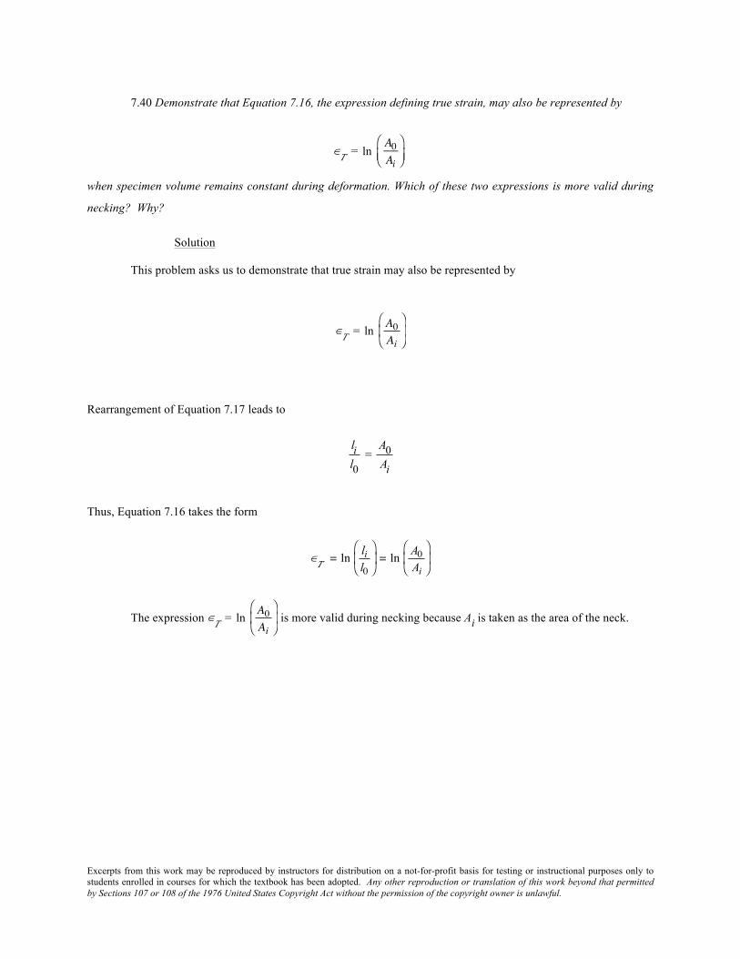
Excerpts from this work may be reproduced by instructors for distribution on a not-for-profit basis for testing or instructional purposes only to students enrolled in courses for which the textbook has been adopted. Any other reproduction or translation of this work beyond that permitted by Sections 107 or 108 of the 1976 United States Copyright Act without the permission of the copyright owner is unlawful.
7.40 Demonstrate that Equation 7.16, the expression defining true strain, may also be represented by
∈T = ln A0Ai
!"#
$%&
when specimen volume remains constant during deformation. Which of these two expressions is more valid during
necking? Why?
Solution
This problem asks us to demonstrate that true strain may also be represented by
∈T = ln
A0Ai
!
" #
$
% &
Rearrangement of Equation 7.17 leads to
lil0
=A0Ai
Thus, Equation 7.16 takes the form
∈T
= ln lil0
!
" #
$
% & = ln
A0Ai
!
" #
$
% &
The expression ∈T = ln
A0Ai
!
" #
$
% & is more valid during necking because Ai is taken as the area of the neck.

Excerpts from this work may be reproduced by instructors for distribution on a not-for-profit basis for testing or instructional purposes only to students enrolled in courses for which the textbook has been adopted. Any other reproduction or translation of this work beyond that permitted by Sections 107 or 108 of the 1976 United States Copyright Act without the permission of the copyright owner is unlawful.
7.41 Using the data in Problem 7.29 and Equations 7.15, 7.16, and 7.18a, generate a true stress–true
strain plot for aluminum. Equation 7.18a becomes invalid past the point at which necking begins; therefore,
measured diameters are given below for the last four data points, which should be used in true stress computations.
Load Length Diameter
N lbf mm in. mm in.
46,100 10,400 56.896 2.240 11.71 0.461
42,400 10,100 57.658 2.270 10.95 0.431
42,600 9,600 58.420 2.300 10.62 0.418
36,400 8,200 59.182 2.330 9.40 0.370
Solution
These true stress-strain data are plotted below.

Excerpts from this work may be reproduced by instructors for distribution on a not-for-profit basis for testing or instructional purposes only to students enrolled in courses for which the textbook has been adopted. Any other reproduction or translation of this work beyond that permitted by Sections 107 or 108 of the 1976 United States Copyright Act without the permission of the copyright owner is unlawful.
7.42 A tensile test is performed on a metal specimen, and it is found that a true plastic strain of 0.20 is
produced when a true stress of 575 MPa (83,500 psi) is applied; for the same metal, the value of K in Equation 7.19
is 860 MPa (125,000 psi). Calculate the true strain that results from the application of a true stress of 600 MPa
(87,000 psi).
Solution
It first becomes necessary to solve for n in Equation 7.19. Taking logarithms of both sides of this
expression leads to
log !T = log K + n log "T
and after rearrangement we have
n =log !T " log K
log #T
And incorporating values of the parameters provided in the problem statement yields
n = log (575 MPa) ! log (860 MPa)log (0.20)
= 0.250
Expressing εT as the dependent variable (Equation 7.19), and then solving for its value from the data stipulated in
the problem statement, leads to
!T = "TK
# $ %
& ' ( 1/n
= 600 MPa860 MPa# $ %
& ' ( 1/0.250
= 0.237

Excerpts from this work may be reproduced by instructors for distribution on a not-for-profit basis for testing or instructional purposes only to students enrolled in courses for which the textbook has been adopted. Any other reproduction or translation of this work beyond that permitted by Sections 107 or 108 of the 1976 United States Copyright Act without the permission of the copyright owner is unlawful.
7.43 For some metal alloy, a true stress of 415 MPa (60,175 psi) produces a plastic true strain of 0.475.
How much will a specimen of this material elongate when a true stress of 325 MPa (46,125 psi) is applied if the
original length is 300 mm (11.8 in.)? Assume a value of 0.25 for the strain-hardening exponent n.
Solution
Solution of this problem requires that we utilize Equation 7.19. It is first necessary to solve for K from the
given true stress and strain. Rearrangement of this equation such that K is the dependent variable yields
K = !T("T )n = 415 MPa
(0.475)0.25 = 500 MPa (72,500 psi)
Next we must solve for the true strain produced when a true stress of 325 MPa is applied, also using Equation 7.19.
Rearrangement of Equation 7.19 such that εT is the dependent variable and incorporation into this expression values
stipulated in the problem statement leads to
!T = "TK
# $ %
& ' ( 1/n
= 325 MPa500 MPa
# $ %
& ' ( 1/0.25
= 0.179 = ln lil0
#
$ %
&
' (
Now, solving for li gives
li = l0e0.179 = (300 mm) e0.179 = 358.8 mm (14.11 in.)
And finally, the elongation ∆l is just
!l = li " l0 = 358.8 mm" 300 mm = 58.8 mm (2.31 in.)

Excerpts from this work may be reproduced by instructors for distribution on a not-for-profit basis for testing or instructional purposes only to students enrolled in courses for which the textbook has been adopted. Any other reproduction or translation of this work beyond that permitted by Sections 107 or 108 of the 1976 United States Copyright Act without the permission of the copyright owner is unlawful.
7.44 The following true stresses produce the corresponding true plastic strains for a brass alloy:
True Stress (psi) True Strain
50,000 0.10
60,000 0.20
What true stress is necessary to produce a true plastic strain of 0.25?
Solution
For this problem, we are given two values of εT and σT, from which we are asked to calculate the true
stress which produces a true plastic strain of 0.25. Taking logarithms of both sides of Equation 7.19 yields
log !T = log K + n log "T
we are able to set up two simultaneous equations with two unknowns (the unknowns being K and n), as
log (50,000 psi) = log K + n log (0.10)
log (60,000 psi) = log K + n log (0.20)
Solving for n from these two expressions yields
n = log (50,000) ! log (60,000)log (0.10) ! log (0.20)
= 0.263
and for K
log K = 4.96 or K = 104.96 = 91,623 psi
Thus, for εT = 0.25
!T = K ("T )n = (91,623 psi)(0.25)0.263 = 63,700 psi (440 MPa)

Excerpts from this work may be reproduced by instructors for distribution on a not-for-profit basis for testing or instructional purposes only to students enrolled in courses for which the textbook has been adopted. Any other reproduction or translation of this work beyond that permitted by Sections 107 or 108 of the 1976 United States Copyright Act without the permission of the copyright owner is unlawful.
7.45 For a brass alloy, the following engineering stresses produce the corresponding plastic engineering
strains prior to necking:
Engineering Stress (MPa) Engineering Strain
235 0.194
250 0.296
On the basis of this information, compute the engineering stress necessary to produce an engineering strain of 0.25.
Solution
For this problem we first need to convert engineering stresses and strains to true stresses and strains so that the constants K and n in Equation 7.19 may be determined. Since σT = σ(1 + ε) (Equation 7.18a) then
!T 1 = (235 MPa)(1 + 0.194) = 280 MPa
!T 2 = (250 MPa)(1 + 0.296) = 324 MPa
Similarly for strains, since εT = ln(1 + ε) (Equation 7.18b) then
!T 1 = ln (1 + 0.194) = 0.177
!T 2 = ln (1 + 0.296) = 0.259
Taking logarithms of Equation 7.19, we get
log !T = log K + n log "T
which allows us to set up two simultaneous equations for the above pairs of true stresses and true strains, with K and
n as unknowns. Thus
log (280) = log K + n log (0.177)
log (324) = log K + n log (0.259)

Excerpts from this work may be reproduced by instructors for distribution on a not-for-profit basis for testing or instructional purposes only to students enrolled in courses for which the textbook has been adopted. Any other reproduction or translation of this work beyond that permitted by Sections 107 or 108 of the 1976 United States Copyright Act without the permission of the copyright owner is unlawful.
Solving for these two expressions yields K = 543 MPa and n = 0.383.
Now, converting ε = 0.25 to true strain (Equation 7.18b)
!T = ln (1 + 0.25) = 0.223
The corresponding σT to give this value of εT (using Equation 7.19) is just
!T = K"Tn = (543 MPa)(0.223)0.383 = 306 MPa
Now converting this value of σT to an engineering stress using Equation 7.18a gives
! = !T1 + "
= 306 MPa1 + 0.25
= 245 MPa

Excerpts from this work may be reproduced by instructors for distribution on a not-for-profit basis for testing or instructional purposes only to students enrolled in courses for which the textbook has been adopted. Any other reproduction or translation of this work beyond that permitted by Sections 107 or 108 of the 1976 United States Copyright Act without the permission of the copyright owner is unlawful.
7.46 Find the toughness (or energy to cause fracture) for a metal that experiences both elastic and plastic
deformation. Assume Equation 7.5 for elastic deformation, that the modulus of elasticity is 172 GPa (25 × 106 psi),
and that elastic deformation terminates at a strain of 0.01. For plastic deformation, assume that the relationship
between stress and strain is described by Equation 7.19, in which the values for K and n are 6900 MPa (1 × 10⁶ psi)
and 0.30, respectively. Furthermore, plastic deformation occurs between strain values of 0.01 and 0.75, at which
point fracture occurs.
Solution
This problem calls for us to compute the toughness (or energy to cause fracture). The easiest way to do this
is to integrate both elastic and plastic regions, and then add them together.
Toughness = ! d"#
= E! d!
0
0.01
" + K!n d!0.01
0.75
"
= E!2
2 0
0.01
+ K(n + 1)
!(n+1)
0.01
0.75
= 172 ! 109 N/m2
2(0.01)2 + 6900 ! 106 N/m2
(1.0 + 0.3)(0.75)1.3 " (0.01)1.3#$ %&
= 3.65 × 10⁹ J/m3 (5.29 × 105 in.-lbf/in.3)

Excerpts from this work may be reproduced by instructors for distribution on a not-for-profit basis for testing or instructional purposes only to students enrolled in courses for which the textbook has been adopted. Any other reproduction or translation of this work beyond that permitted by Sections 107 or 108 of the 1976 United States Copyright Act without the permission of the copyright owner is unlawful.
7.47 For a tensile test, it can be demonstrated that necking begins when
d!Td"T
= !T (7.31)
Using Equation 7.19, determine the value of the true strain at this onset of necking.
Solution
Let us take the derivative of Equation 7.19, set it equal to σT, and then solve for εT from the resulting
expression. Thus
d K (!T )n"# $%d!T
= Kn(!T )(n&1) = 'T
However, from Equation 7.19, σT = K(εT)n, which, when substituted into the above expression, yields
Kn (!T )(n - 1) = K (!T )
n
Now solving for εT from this equation leads to
εT = n
as the value of the true strain at the onset of necking.

Excerpts from this work may be reproduced by instructors for distribution on a not-for-profit basis for testing or instructional purposes only to students enrolled in courses for which the textbook has been adopted. Any other reproduction or translation of this work beyond that permitted by Sections 107 or 108 of the 1976 United States Copyright Act without the permission of the copyright owner is unlawful.
7.48 Taking the logarithm of both sides of Equation 7.19 yields
log !T = log K + n log "T (7.32)
Thus, a plot of log σT versus log ∈T in the plastic region to the point of necking should yield a straight line having a
slope of n and an intercept (at log σT = 0) of log K.
Using the appropriate data tabulated in Problem 7.29, make a plot of log σT versus log ∈T and determine
the values of n and K. It will be necessary to convert engineering stresses and strains to true stresses and strains
using Equations 7.18a and 7.18b.
Solution
This problem calls for us to utilize the appropriate data from Problem 7.29 in order to determine the values of n and K for this material. From Equation 7.32 the slope and intercept of a log σT versus log εT plot will yield n
and log K, respectively. However, Equation 7.19 is only valid in the region of plastic deformation to the point of
necking; thus, only the 7th, 8th, 9th, and 10th data points may be utilized. The log-log plot with these data points is
given below.
The slope yields a value of 0.136 for n, whereas the intercept gives a value of 2.7497 for log K, and thus K =
102.7497 = 562 MPa.

Excerpts from this work may be reproduced by instructors for distribution on a not-for-profit basis for testing or instructional purposes only to students enrolled in courses for which the textbook has been adopted. Any other reproduction or translation of this work beyond that permitted by Sections 107 or 108 of the 1976 United States Copyright Act without the permission of the copyright owner is unlawful.
Elastic Recovery after Plastic Deformation
7.49 A cylindrical specimen of a brass alloy 7.5 mm (0.30 in.) in diameter and 90.0 mm (3.54 in.) long is
pulled in tension with a force of 6000 N (1350 lbf); the force is subsequently released.
(a) Compute the final length of the specimen at this time. The tensile stress–strain behavior for this alloy is
shown in Figure 7.12.
(b) Compute the final specimen length when the load is increased to 16,500 N (3700 lbf) and then released.
Solution
(a) In order to determine the final length of the brass specimen when the load is released, it first becomes
necessary to compute the applied stress using Equation 7.1; thus
! = FA0
= F
" d02
# $ %
& ' (
2 = 6000 N
" 7.5 ) 10*3 m2
#
$ %
&
' (
2 = 136 MPa (19,000 psi)
Upon locating this point on the stress-strain curve (Figure 7.12), we note that it is in the linear, elastic region;
therefore, when the load is released the specimen will return to its original length of 90 mm (3.54 in.).
(b) In this portion of the problem we are asked to calculate the final length, after load release, when the load is increased to 16,500 N (3700 lbf). Again, computing the stress
! = 16,500 N
" 7.5 # 10$3 m2
%
& '
(
) * 2 = 373 MPa (52,300 psi)
The point on the stress-strain curve corresponding to this stress is in the plastic region. We are able to estimate the
amount of permanent strain by drawing a straight line parallel to the linear elastic region; this line intersects the strain axis at a strain of about 0.08, which is the amount of plastic strain. The final specimen length li may be
determined from a rearranged form of Equation 7.2 as
li = l0(1 + ε) = (90 mm)(1 + 0.08) = 97.20 mm (3.82 in.)

Excerpts from this work may be reproduced by instructors for distribution on a not-for-profit basis for testing or instructional purposes only to students enrolled in courses for which the textbook has been adopted. Any other reproduction or translation of this work beyond that permitted by Sections 107 or 108 of the 1976 United States Copyright Act without the permission of the copyright owner is unlawful.
7.50 A steel alloy specimen having a rectangular cross section of dimensions 12.7 mm × 6.4 mm (0.5 in. ×
0.25 in.) has the stress–strain behavior shown in Figure 7.33. This specimen is subjected to a tensile force of 38,000
N (8540 lbf).
(a) Determine the elastic and plastic strain values.
(b) If its original length is 460 mm (18.0 in.), what will be its final length after the load in part (a) is
applied and then released?
Solution
(a) We are asked to determine both the elastic and plastic strain values when a tensile force of 38,000 N (8540 lbf) is applied to the steel specimen and then released. First it becomes necessary to determine the applied
stress using Equation 7.1; thus
! = FA0
= Fb0d0
where b0 and d0 are cross-sectional width and depth (12.7 mm and 6.4 mm, respectively). Thus
! = 38,000 N(12.7 " 10#3 m)(6.4 " 10#3 m) = 468 " 106 N /m2 = 468 MPa (68,300 psi)
From Figure 7.33, this point is in the plastic region so the specimen will be both elastic and plastic strains. The total strain at this point, εt, is about 0.010. We are able to estimate the amount of permanent strain recovery εe from
Hooke's law, Equation 7.5 as
!e = "E
And since E = 207 GPa for steel (Table 7.1)
!e = 468 MPa207 " 103 MPa
= 0.00226
The value of the plastic strain, εp, is just the difference between the total and elastic strains; that is
εp = εt – εe = 0.010 – 0.00226 = 0.00774

Excerpts from this work may be reproduced by instructors for distribution on a not-for-profit basis for testing or instructional purposes only to students enrolled in courses for which the textbook has been adopted. Any other reproduction or translation of this work beyond that permitted by Sections 107 or 108 of the 1976 United States Copyright Act without the permission of the copyright owner is unlawful.
(b) If the initial length is 460 mm (18.0 in.) then the final specimen length li may be determined from a
rearranged form of Equation 7.2 using the plastic strain value as
li = l0(1 + εp) = (460 mm)(1 + 0.00774) = 463.6 mm (18.14 in.)
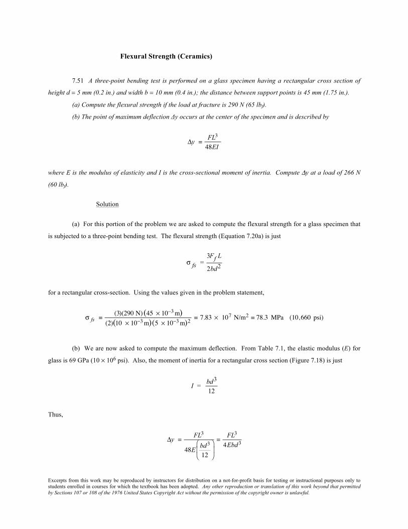
Excerpts from this work may be reproduced by instructors for distribution on a not-for-profit basis for testing or instructional purposes only to students enrolled in courses for which the textbook has been adopted. Any other reproduction or translation of this work beyond that permitted by Sections 107 or 108 of the 1976 United States Copyright Act without the permission of the copyright owner is unlawful.
Flexural Strength (Ceramics)
7.51 A three-point bending test is performed on a glass specimen having a rectangular cross section of
height d = 5 mm (0.2 in.) and width b = 10 mm (0.4 in.); the distance between support points is 45 mm (1.75 in.).
(a) Compute the flexural strength if the load at fracture is 290 N (65 lbf).
(b) The point of maximum deflection Δy occurs at the center of the specimen and is described by
!y = FL3
48EI
where E is the modulus of elasticity and I is the cross-sectional moment of inertia. Compute Δy at a load of 266 N
(60 lbf).
Solution
(a) For this portion of the problem we are asked to compute the flexural strength for a glass specimen that
is subjected to a three-point bending test. The flexural strength (Equation 7.20a) is just
! fs =3Ff L
2bd2
for a rectangular cross-section. Using the values given in the problem statement,
! fs = (3)(290 N)(45 " 10#3 m)(2)(10 " 10#3 m)(5 " 10#3 m)2 = 7.83 " 107 N/m2 = 78.3 MPa (10,660 psi)
(b) We are now asked to compute the maximum deflection. From Table 7.1, the elastic modulus (E) for
glass is 69 GPa (10 × 106 psi). Also, the moment of inertia for a rectangular cross section (Figure 7.18) is just
I = bd3
12
Thus,
!y = FL3
48E bd3
12
"
# $
%
& '
= FL3
4Ebd3

Excerpts from this work may be reproduced by instructors for distribution on a not-for-profit basis for testing or instructional purposes only to students enrolled in courses for which the textbook has been adopted. Any other reproduction or translation of this work beyond that permitted by Sections 107 or 108 of the 1976 United States Copyright Act without the permission of the copyright owner is unlawful.
= (266 N)(45 ! 10"3 m)3
(4)(69 ! 109 N/m2)(10 ! 10"3 m)(5 ! 10"3 m)3
= 7.0 × 10⁻⁵ m = 7.0 × 10⁻² mm (2.5 × 10⁻³ in.)

Excerpts from this work may be reproduced by instructors for distribution on a not-for-profit basis for testing or instructional purposes only to students enrolled in courses for which the textbook has been adopted. Any other reproduction or translation of this work beyond that permitted by Sections 107 or 108 of the 1976 United States Copyright Act without the permission of the copyright owner is unlawful.
7.52 A circular specimen of MgO is loaded using a three-point bending mode. Compute the minimum
possible radius of the specimen without fracture, given that the applied load is 425 N (95.5 lbf), the flexural strength
is 105 MPa (15,000 psi), and the separation between load points is 50 mm (2.0 in.).
Solution
We are asked to calculate the maximum radius of a circular specimen of MgO that is loaded using three-
point bending. Solving for R from Equation 7.20b
R =Ff L
! fs"
#
$ % %
&
' ( (
1/3
which, when substituting the parameters stipulated in the problem statement, yields
R = (425 N)(50 ! 10"3 m)(105 ! 106 N /m2)(#)
$
% &
'
( ) 1/3
= 4.0 × 10⁻³ m = 4.0 mm (0.16 in.)

Excerpts from this work may be reproduced by instructors for distribution on a not-for-profit basis for testing or instructional purposes only to students enrolled in courses for which the textbook has been adopted. Any other reproduction or translation of this work beyond that permitted by Sections 107 or 108 of the 1976 United States Copyright Act without the permission of the copyright owner is unlawful.
7.53 A three-point bending test was performed on an aluminum oxide specimen having a circular cross
section of radius 3.5 mm (0.14 in.); the specimen fractured at a load of 950 N (215 lbf) when the distance between
the support points was 50 mm (2.0 in.). Another test is to be performed on a specimen of this same material, but one
that has a square cross section of 12 mm (0.47 in.) length on each edge. At what load would you expect this
specimen to fracture if the support point separation is 40 mm (1.6 in.)?
Solution
For this problem, the load is given at which a circular specimen of aluminum oxide fractures when
subjected to a three-point bending test; we are then are asked to determine the load at which a specimen of the same
material having a square cross-section fractures. It is first necessary to compute the flexural strength of the aluminum oxide, Equation 7.20b, and then, using this value, we may calculate the value of Ff in Equation 7.20a.
From Equation 7.20b
! fs =
Ff L"R3
= (950 N)(50 ! 10"3 m)(#) (3.5 ! 10"3 m)3 = 352 ! 106 N/m2 = 352 MPa (50,000 psi)
Now, solving for Ff from Equation 7.20a, realizing that b = d = 12 mm, yields
Ff =
2! fsd 3
3L
= (2) (352 ! 106 N /m2)(12 ! 10"3 m)3(3) (40 ! 10"3 m) = 10,100 N (2165 lbf )

Excerpts from this work may be reproduced by instructors for distribution on a not-for-profit basis for testing or instructional purposes only to students enrolled in courses for which the textbook has been adopted. Any other reproduction or translation of this work beyond that permitted by Sections 107 or 108 of the 1976 United States Copyright Act without the permission of the copyright owner is unlawful.
7.54 (a) A three-point transverse bending test is conducted on a cylindrical specimen of aluminum oxide
having a reported flexural strength of 390 MPa (56,600 psi). If the specimen radius is 2.5 mm (0.10 in.) and the
support point separation distance is 30 mm (1.2 in.), would you expect the specimen to fracture when a load of 620
N (140 lbf) is applied? Justify your answer.
(b) Would you be 100% certain of the answer in part (a)? Why or why not?
Solution
(a) This portion of the problem asks that we determine whether or not a cylindrical specimen of aluminum
oxide having a flexural strength of 390 MPa (56,600 psi) and a radius of 2.5 mm will fracture when subjected to a
load of 620 N in a three-point bending test; the support point separation is given as 30 mm. Using Equation 7.30b we will calculate the value of σ; if this value is greater than σfs (390 MPa), then fracture is expected to occur.
Employment of Equation 7.30b yields
! = FL"R3
= (620 N)(30 ! 10"3 m)(#) (2.5 ! 10"3 m)3 = 379 ! 106 N/m2 = 379 MPa (53,500 psi)
Since this value is less than the given value of σfs (390 MPa), then fracture is not predicted.
(b) The certainty of this prediction is not 100% because there is always some variability in the flexural strength for ceramic materials, and since this value of σ (379 MPa) is relatively close to σfs (390 MPa) then there is
some chance that fracture will occur.

Excerpts from this work may be reproduced by instructors for distribution on a not-for-profit basis for testing or instructional purposes only to students enrolled in courses for which the textbook has been adopted. Any other reproduction or translation of this work beyond that permitted by Sections 107 or 108 of the 1976 United States Copyright Act without the permission of the copyright owner is unlawful.
Influence of Porosity on the Mechanical Properties of Ceramics
7.55 The modulus of elasticity for beryllium oxide (BeO) having 5 vol% porosity is 310 GPa (45 × 106 psi).
(a) Compute the modulus of elasticity for the nonporous material.
(b) Compute the modulus of elasticity for 10 vol% porosity.
Solution
(a) This portion of the problem requests that we compute the modulus of elasticity for nonporous BeO given that E = 310 GPa for a material having 5 vol% porosity. Thus, we solve Equation 7.21 for E0, using P = 0.05,
which gives
E0 = E1 ! 1.9P + 0.9P2
= 310 GPa1 ! (1.9)(0.05) + (0.9)(0.05)2 = 342 GPa (49.6 " 106 psi)
(b) Now we are asked to determine the value of E at P = 10 vol% (i.e., 0.10). Using Equation 7.21 we get
E = E0(1 ! 1.9P + 0.9P2)
= (342 GPa) 1 ! (1.9)(0.10) + (0.9)(0.10)2"# $% = 280 GPa (40.6 & 106 psi)

Excerpts from this work may be reproduced by instructors for distribution on a not-for-profit basis for testing or instructional purposes only to students enrolled in courses for which the textbook has been adopted. Any other reproduction or translation of this work beyond that permitted by Sections 107 or 108 of the 1976 United States Copyright Act without the permission of the copyright owner is unlawful.
7.56 The modulus of elasticity for boron carbide (B4C) having 5 vol% porosity is 290 GPa (42 × 106 psi).
(a) Compute the modulus of elasticity for the nonporous material.
(b) At what volume percent porosity will the modulus of elasticity be 235 GPa (34 × 106 psi)?
Solution
(a) This portion of the problem requests that we compute the modulus of elasticity for nonporous B4C
given that E = 290 GPa (42 × 106 psi) for a material having 5 vol% porosity. Thus, we solve Equation 7.21 for E0,
using P = 0.05, which gives
E0 = E1 ! 1.9P + 0.9P2
= 290 GPa1 ! (1.9)(0.05) + (0.9)(0.05)2 = 320 GPa (46.3 " 106 psi)
(b) Now we are asked to compute the volume percent porosity at which the elastic modulus of B4C is 235
MPa (34 × 106 psi). Since from part (a), E0 = 320 GPa, and using Equation 7.21 we get
EE0
= 235 MPa320 MPa
= 0.734 = 1 ! 1.9P + 0.9P2
Or
0.9P2 ! 1.9P + 0.266 = 0
Now, solving for the value of P using the quadratic equation solution yields
P =1.9 ± (!1.9)2 ! (4)(0.9)(0.266)
(2)(0.9)
The positive and negative roots are
P+ = 1.96
P- = 0.151
Obviously, only the negative root is physically meaningful, and therefore the value of the porosity to give the
desired modulus of elasticity is 15.1 vol%.

Excerpts from this work may be reproduced by instructors for distribution on a not-for-profit basis for testing or instructional purposes only to students enrolled in courses for which the textbook has been adopted. Any other reproduction or translation of this work beyond that permitted by Sections 107 or 108 of the 1976 United States Copyright Act without the permission of the copyright owner is unlawful.
7.57 Using the data in Table 7.2, do the following:
(a) Determine the flexural strength for nonporous MgO assuming a value of 3.75 for n in Equation 7.22.
(b) Compute the volume fraction porosity at which the flexural strength for MgO is 62 MPa (9000 psi).
Solution
(a) This part of the problem asks us to determine the flexural strength of nonporous MgO assuming that the
value of n in Equation 7.22 is 3.75. Taking natural logarithms of both sides of Equation 7.22 yields
ln ! fs = ln!0 " nP
In Table 7.2 it is noted that for P = 0.05, σfs = 105 MPa. For the nonporous material P = 0 and ln σ0 = ln σ .
Solving for ln σ0 from the above equation and using these data gives
ln!0 = ln! fs + nP
= ln (105 MPa) + (3.75)(0.05) = 4.841
or σ0 = e4.841 = 127 MPa (18,100 psi)
(b) Now we are asked to compute the volume percent porosity to yield a σfs of 62 MPa (9000 psi). Taking
the natural logarithm of Equation 7.22 and solving for P leads to
P =ln !0 " ln ! fs
n
= ln (127 MPa) ! ln (62 MPa)3.75
= 0.19 or 19 vol%

Excerpts from this work may be reproduced by instructors for distribution on a not-for-profit basis for testing or instructional purposes only to students enrolled in courses for which the textbook has been adopted. Any other reproduction or translation of this work beyond that permitted by Sections 107 or 108 of the 1976 United States Copyright Act without the permission of the copyright owner is unlawful.
7.58 The flexural strength and associated volume fraction porosity for two specimens of the same ceramic
material are as follows:
σfs (MPa) P
100 0.05
50 0.20
(a) Compute the flexural strength for a completely nonporous specimen of this material.
(b) Compute the flexural strength for a 0.10 volume fraction porosity.
Solution
(a) Given the flexural strengths at two different volume fraction porosities, we are asked to determine the
flexural strength for a nonporous material. If the natural logarithm is taken of both sides of Equation 7.22, then
ln! fs = ln!0 " nP
Using the data provided in the problem statement, two simultaneous equations may be written as
ln (100 MPa) = ln !0 " (0.05) n
ln (50 MPa) = ln !0 " (0.20) n
Solving for n and σ0 leads to n = 4.62 and σ0 = 126 MPa. For the nonporous material, P = 0, and from Equation
7.22, σ0 = σfs. Thus, σfs for P = 0 is 126 MPa.
(b) Now, we are asked for σfs at P = 0.10 for this same material. Utilizing Equation 7.22 yields
! fs = !0 exp (" nP)
= (126 MPa) exp ! (4.62)(0.10)[ ]
= 79.4 MPa

Excerpts from this work may be reproduced by instructors for distribution on a not-for-profit basis for testing or instructional purposes only to students enrolled in courses for which the textbook has been adopted. Any other reproduction or translation of this work beyond that permitted by Sections 107 or 108 of the 1976 United States Copyright Act without the permission of the copyright owner is unlawful.
Stress-Strain Behavior (Polymers)
7.59 From the stress–strain data for poly(methyl methacrylate) shown in Figure 7.24, determine the
modulus of elasticity and tensile strength at room temperature [20°C (68°F)], and compare these values with those
given in Tables 7.1 and 7.2.
Solution
From Figure 7.24, the elastic modulus is the slope in the elastic linear region of the 20°C curve, which is
E = ! (stress)
! (strain)= 30 MPa " 0 MPa
9 # 10"3 " 0= 3.3 GPa (483,000 psi)
The value range cited in Table 7.1 is 2.24 to 3.24 GPa (325,000 to 470,000 psi). Thus, the plotted value is a little on
the high side.
The tensile strength corresponds to the stress at which the curve ends, which is 52 MPa (7500 psi). This
value lies within the range cited in Table 7.2—48.3 to 72.4 MPa (7000 to 10,500 psi).

Excerpts from this work may be reproduced by instructors for distribution on a not-for-profit basis for testing or instructional purposes only to students enrolled in courses for which the textbook has been adopted. Any other reproduction or translation of this work beyond that permitted by Sections 107 or 108 of the 1976 United States Copyright Act without the permission of the copyright owner is unlawful.
7.60 Compute the elastic moduli for the following polymers, whose stress-strain behaviors can be observed
in the Tensile Tests module of Virtual Materials Science and Engineering (VMSE): (a) high-density polyethylene,
(b) nylon, and (c) phenol-formaldehyde (bakelite). How do these values compare with those presented in Table 7.1
for the same polymers?
Solution
The elastic modulus is the slope in the linear elastic region (Equation 7.10) as
E = !"!#
= "2 $ "1#2 $ #1
Since all the stress-strain curves pass through the origin, we make take σ1 = 0 and ε1 = 0. Determinations of σ2 and
ε2 are possible by moving the cursor to some arbitrary point in the linear region of the curve and then reading
corresponding values in the “Stress” and “Strain” windows that are located below the plot.
(a) A screenshot for the high-density polyethylene in the elastic region is shown below.
Here the cursor point resides in the elastic region at a stress of 10.9 MPa (which is the value of σ2) at a strain of
0.0318 (which is the value of ε2). Thus, the elastic modulus is equal to

Excerpts from this work may be reproduced by instructors for distribution on a not-for-profit basis for testing or instructional purposes only to students enrolled in courses for which the textbook has been adopted. Any other reproduction or translation of this work beyond that permitted by Sections 107 or 108 of the 1976 United States Copyright Act without the permission of the copyright owner is unlawful.
E = ! 2 " !1
#2 " #1 = 10.9 MPa " 0 MPa
0.0318 " 0 = 343 MPa = 0.343 GPa
The elastic modulus for high-density polyethylene given in Table 7.1 is 1.08 GPa, which is significantly
higher than this value.
(b) A screenshot for the nylon in the elastic region is shown below.
Here the cursor point resides in the elastic region at a stress of 53.3 MPa (which is the value of σ2) at a strain of
0.0204 (which is the value of ε2). Thus, the elastic modulus is equal to
E = ! 2 " !1
#2 " #1 = 53.3 MPa " 0 MPa
0.0204 " 0 = 2,610 MPa = 2.61 GPa
The elastic modulus range for nylon 6,6 given in Table 7.1 is 1.59 GPa to 3.79 GPa; therefore, the value
for the VMSE nylon lies within this range.
(c) A screenshot for the Bakelite in the elastic region is shown below.

Excerpts from this work may be reproduced by instructors for distribution on a not-for-profit basis for testing or instructional purposes only to students enrolled in courses for which the textbook has been adopted. Any other reproduction or translation of this work beyond that permitted by Sections 107 or 108 of the 1976 United States Copyright Act without the permission of the copyright owner is unlawful.
Here the cursor point resides in the elastic region at a stress of 40.8 MPa (which is the value of σ2) at a strain of
0.0085 (which is the value of ε2). Thus, the elastic modulus is equal to
E = ! 2 " !1
#2 " #1 = 40.8 MPa " 0 MPa
0.0085 " 0 = 4,800 MPa = 4.8 GPa
The elastic modulus range for the Bakelite given in Table 7.1 is 2.76 GPa to 4.83 GPa; therefore, this value
for the VMSE Bakelite lies just below the maximum value for this range.

Excerpts from this work may be reproduced by instructors for distribution on a not-for-profit basis for testing or instructional purposes only to students enrolled in courses for which the textbook has been adopted. Any other reproduction or translation of this work beyond that permitted by Sections 107 or 108 of the 1976 United States Copyright Act without the permission of the copyright owner is unlawful.
7.61 For the nylon polymer whose stress-strain behavior can be observed in the Tensile Tests module of
Virtual Materials Science and Engineering (VMSE), determine the following:
(a) The yield strength.
(b) The approximate ductility, in percent elongation.
How do these values compare with those for the nylon material presented in Table 7.2?
Solution
A screenshot of the stress-strain curve for nylon (to fracture) is shown below.
(a) The yield strength corresponds to the first maximum (just beyond the initial linear-elastic region) of the
stress-strain curve; as noted in this plot, the value is 84 MPa.
(b) The approximate percent elongation corresponds to the strain at fracture (“0.445” as noted in the
“Strain” box) multiplied by 100 (i.e., 44.5%) minus the maximum elastic strain (i.e., value of strain at which the
linearity of the curve ends multiplied by 100—in this case about 4%); this gives a value of about 40%EL.
For nylon 6,6, the range of values of yield strength presented in Table 7.2 is 44.8 MPa to 82.8 MPa;
therefore, the value for the VMSE nylon lies slightly above the upper value. The ductility range for nylon 6,6 is
15%EL to 300%EL; therefore, our value (40%EL) lies within this range.

Excerpts from this work may be reproduced by instructors for distribution on a not-for-profit basis for testing or instructional purposes only to students enrolled in courses for which the textbook has been adopted. Any other reproduction or translation of this work beyond that permitted by Sections 107 or 108 of the 1976 United States Copyright Act without the permission of the copyright owner is unlawful.
7.62 For the phenol-formaldehyde (Bakelite) polymer whose stress strain behavior can be observed in the
Tensile Tests module of Virtual Materials Science and Engineering (VMSE), determine the following:
(a) The tensile strength.
(b) The approximate ductility, in percent elongation.
How do these values compare with those for the phenol-formaldehyde material presented in Table 7.2?
Solution
A screenshot of the stress-strain curve for phenol-fornaldehyde (to fracture) is shown below.
(a) The tensile strength corresponds to the stress at which fracture occurs. This reading in the stress
window located below this plot at the point of fracture—the tensile strength—is 52 MPa.
(b) The approximate percent elongation corresponds to the strain at fracture (“0.0129” as noted in the
“Strain” box) multiplied by 100 (i.e., 1.29%) minus the maximum elastic strain (i.e., value of strain at which the
linearity of the curve ends multiplied by 100—in this case about 1%); this gives a value of about 0.29%EL.
For phenol-formaldehyde, the range of values of tensile strength presented in Table 7.2 is 34.5 MPa to 62.1
MPa; therefore, the value for the VMSE material (52 MPa) lies within this range. The ductility range for phenol-
formaldehyde is 1.5%EL to 2.0%EL; therefore, our value (0.3%EL) lies below the lower limit.

Excerpts from this work may be reproduced by instructors for distribution on a not-for-profit basis for testing or instructional purposes only to students enrolled in courses for which the textbook has been adopted. Any other reproduction or translation of this work beyond that permitted by Sections 107 or 108 of the 1976 United States Copyright Act without the permission of the copyright owner is unlawful.
Viscoelastic Deformation
7.63 In your own words, briefly describe the phenomenon of viscoelasticity.
The explanation of viscoelasticity is given in Section 7.15.

Excerpts from this work may be reproduced by instructors for distribution on a not-for-profit basis for testing or instructional purposes only to students enrolled in courses for which the textbook has been adopted. Any other reproduction or translation of this work beyond that permitted by Sections 107 or 108 of the 1976 United States Copyright Act without the permission of the copyright owner is unlawful.
7.64 For some viscoelastic polymers that are subjected to stress relaxation tests, the stress decays with
time according to
!(t) = !(0) exp " t#
$ % &
' ( ) (7.33)
where σ(t) and σ(0) represent the time-dependent and initial (i.e., time = 0) stresses, respectively, and t and τ denote
elapsed time and the relaxation time, respectively; τ is a time-independent constant characteristic of the material. A
specimen of some viscoelastic polymer whose stress relaxation obeys Equation 7.33 was suddenly pulled in tension
to a measured strain of 0.6; the stress necessary to maintain this constant strain was measured as a function of time.
Determine Er(10) for this material if the initial stress level was 2.76 MPa (400 psi), which dropped to 1.72 MPa
(250 psi) after 60 s.
Solution
This problem asks for a determination of the relaxation modulus of a viscoelastic material, which behavior
is according to Equation 7.33—i.e.,
!(t) = !(0) exp " t#
$ % &
' ( )
We want to determine σ(10), but it is first necessary to compute τ from the data provided in the problem statement.
Taking natural logarithms of both sides of Equation 7.33 gives the following:
ln ! (t) = ln ! (0) " t
#
Thus, solving for τ from the above expression and incorporating values for σ(0) and σ(t) provided in the problem
statement, yields
! = " t
ln # (t)# (0)$%&
'()
= "60 s
ln 1.72 MPa2.76 MPa
$%&
'()
= 127 s
Therefore, from Equation 7.33 the value of σ(10) is equal to
! (10) = (2.76 MPa) exp " 10 s127 s
#$%
&'( = 2.55 MPa

Excerpts from this work may be reproduced by instructors for distribution on a not-for-profit basis for testing or instructional purposes only to students enrolled in courses for which the textbook has been adopted. Any other reproduction or translation of this work beyond that permitted by Sections 107 or 108 of the 1976 United States Copyright Act without the permission of the copyright owner is unlawful.
Now, using Equation 7.23, we solve for Er(10) as follows:
Er (10) = ! (10)"0
= 2.55 MPa0.6
= 4.25 MPa (616 psi)

Excerpts from this work may be reproduced by instructors for distribution on a not-for-profit basis for testing or instructional purposes only to students enrolled in courses for which the textbook has been adopted. Any other reproduction or translation of this work beyond that permitted by Sections 107 or 108 of the 1976 United States Copyright Act without the permission of the copyright owner is unlawful.
7.65 In Figure 7.35, the logarithm of Er(t) versus the logarithm of time is plotted for polyisobutylene at a
variety of temperatures. Plot Er(10) versus temperature and then estimate its Tg.
Solution
Below is plotted the logarithm of Er(10) versus temperature.
The glass-transition temperature is that temperature corresponding to the abrupt decrease in log Er(10), which for
this polyisobutylene material is about −60°C.

Excerpts from this work may be reproduced by instructors for distribution on a not-for-profit basis for testing or instructional purposes only to students enrolled in courses for which the textbook has been adopted. Any other reproduction or translation of this work beyond that permitted by Sections 107 or 108 of the 1976 United States Copyright Act without the permission of the copyright owner is unlawful.
7.66 On the basis of the curves in Figure 7.26, sketch schematic strain–time plots for the following
polystyrene materials at the specified temperatures:
(a) Amorphous at 120°C
(b) Crosslinked at 150°C
(c) Crystalline at 230°C
(d) Crosslinked at 50°C
Solution
(a) Amorphous polystyrene at 120°C behaves as a rubbery material (Figure 7.29, curve C); therefore, the
strain-time behavior would be as Figure 7.26c.
(b) Crosslinked polystyrene at 150°C behaves as a viscoelastic material (Figure 7.29, curve B); therefore,
the strain-time behavior will be as Figure 7.26c.
(c) Crystalline polystyrene at 230°C behaves as a viscous liquid (Figure 7.29, curve A); therefore, the
strain-time behavior will be as Figure 7.26d.
(d) Crosslinked polystyrene at 50°C behaves in a glassy manner (Figure 7.29, curve B); therefore, the
strain-time behavior will be as Figure 7.26b.

Excerpts from this work may be reproduced by instructors for distribution on a not-for-profit basis for testing or instructional purposes only to students enrolled in courses for which the textbook has been adopted. Any other reproduction or translation of this work beyond that permitted by Sections 107 or 108 of the 1976 United States Copyright Act without the permission of the copyright owner is unlawful.
7.67 (a) Contrast the manner in which stress relaxation and viscoelastic creep tests are conducted.
(b) For each of these tests, cite the experimental parameter of interest and how it is determined.
Solution
(a) Stress relaxation tests are conducted by rapidly straining the material elastically in tension, holding the
strain level constant, and then measuring the stress as a function of time. For viscoelastic creep tests, a stress
(usually tensile) is applied instantaneously and maintained constant while strain is measured as a function of time.
(b) The experimental parameters of interest from the stress relaxation and viscoelastic creep tests are the
relaxation modulus and creep modulus (or creep compliance), respectively. The relaxation modulus is the ratio of
stress measured after 10 s and strain (Equation 7.23); creep modulus is the ratio of stress and strain taken at a
specific time (Equation 7.24).

Excerpts from this work may be reproduced by instructors for distribution on a not-for-profit basis for testing or instructional purposes only to students enrolled in courses for which the textbook has been adopted. Any other reproduction or translation of this work beyond that permitted by Sections 107 or 108 of the 1976 United States Copyright Act without the permission of the copyright owner is unlawful.
7.68 Make two schematic plots of the logarithm of relaxation modulus versus temperature for an
amorphous polymer (curve C in Figure 7.29).
(a) On one of these plots demonstrate how the behavior changes with increasing molecular weight.
(b) On the other plot, indicate the change in behavior with increasing crosslinking.
Solution
(a) This portion of the problem calls for a plot of log Er(10) versus temperature demonstrating how the
behavior changes with increased molecular weight. Such a plot is given below. Increasing molecular weight
increases both glass-transition and melting temperatures.
(b) We are now called upon to make a plot of log Er(10) versus temperature demonstrating how the
behavior changes with increased crosslinking. Such a plot is given below. Increasing the degree of crosslinking
will increase the modulus in both glassy and rubbery regions.

Excerpts from this work may be reproduced by instructors for distribution on a not-for-profit basis for testing or instructional purposes only to students enrolled in courses for which the textbook has been adopted. Any other reproduction or translation of this work beyond that permitted by Sections 107 or 108 of the 1976 United States Copyright Act without the permission of the copyright owner is unlawful.
Hardness
7.69 (a) A 10-mm-diameter Brinell hardness indenter produced an indentation 1.62 mm in diameter in a
steel alloy when a load of 500 kg was used. Compute the HB of this material.
(b) What will be the diameter of an indentation to yield a hardness of 450 HB when a 500-kg load is used?
Solution
(a) We are asked to compute the Brinell hardness for the given indentation. It is necessary to use the
equation in Table 7.5 for HB, where P = 500 kg, d = 1.62 mm, and D = 10 mm. Thus, the Brinell hardness is
computed as
HB = 2P
! D D " D2 " d2#$%
&'(
= (2)(500 kg)
(!)(10 mm) 10 mm " (10 mm)2 " (1.62 mm)2#$%
&'(
= 241
(b) This part of the problem calls for us to determine the indentation diameter d which will yield a 450 HB
when P = 500 kg. Solving for d from the equation in Table 7.5 gives
d = D2 ! D ! 2P(HB)"D
#
$ %
&
' ( 2
= (10mm)2 ! 10 mm ! (2)(500 kg)(450)(")(10 mm)
# $ %
& ' ( 2
= 1.19 mm

Excerpts from this work may be reproduced by instructors for distribution on a not-for-profit basis for testing or instructional purposes only to students enrolled in courses for which the textbook has been adopted. Any other reproduction or translation of this work beyond that permitted by Sections 107 or 108 of the 1976 United States Copyright Act without the permission of the copyright owner is unlawful.
7.70 Estimate the Brinell and Rockwell hardnesses for the following:
(a) The naval brass for which the stress-strain behavior is shown in Figure 7.12.
(b) The steel alloy for which the stress-strain behavior is shown in Figure 7.33.
Solution
This problem calls for estimations of Brinell and Rockwell hardnesses.
(a) For the brass specimen, the stress-strain behavior for which is shown in Figure 7.12, the tensile strength
is calculated in Example Problem 7.3; its value is 450 MPa (65,000 psi). From Figure 7.31, the hardness for brass
corresponding to this tensile strength is about 125 HB or 70 HRB.
(b) The steel alloy (Figure 7.33) has a tensile strength of about 515 MPa (74,700 psi) [Problem 7.25(d)].
This corresponds to a hardness of about 160 HB or ~90 HRB from the line for steels in Figure 7.1. Alternately,
using Equation 7.25a
HB = TS(MPa)3.45
= 515 MPa3.45
= 149

Excerpts from this work may be reproduced by instructors for distribution on a not-for-profit basis for testing or instructional purposes only to students enrolled in courses for which the textbook has been adopted. Any other reproduction or translation of this work beyond that permitted by Sections 107 or 108 of the 1976 United States Copyright Act without the permission of the copyright owner is unlawful.
7.71 Using the data represented in Figure 7.31, specify equations relating tensile strength and Brinell
hardness for brass and nodular cast iron, similar to Equations 7.25a and 7.25b for steels.
Solution
These equations, for a straight line, are of the form
TS = C + (E)(HB)
where TS is the tensile strength, HB is the Brinell hardness, and C and E are constants, which need to be determined.
One way to solve for C and E is analytically—establishing two equations using TS and HB data points on
the plot, as
(TS)1 = C + (E)(BH)1
(TS)2 = C + (E)(BH)2
Solving for E from these two expressions yields
E =(TS)1 ! (TS)2(HB)2 ! (HB)1
For nodular cast iron, if we make the arbitrary choice of (HB)1 and (HB)2 as 200 and 300, respectively, then from
Figure 7.31, (TS)1 and (TS)2 take on values of 600 MPa (87,000 psi) and 1100 MPa (160,000 psi), respectively.
Substituting these values into the above expression and solving for E gives
E = 600 MPa ! 1100 MPa200 HB ! 300 HB
= 5.0 MPa/HB (730 psi/HB)
Now, solving for C yields
C = (TS)1 – (E)(BH)1
= 600 MPa − (5.0 MPa/HB)(200 HB) = – 400 MPa (– 59,000 psi)
Thus, for nodular cast iron, these two equations take the form

Excerpts from this work may be reproduced by instructors for distribution on a not-for-profit basis for testing or instructional purposes only to students enrolled in courses for which the textbook has been adopted. Any other reproduction or translation of this work beyond that permitted by Sections 107 or 108 of the 1976 United States Copyright Act without the permission of the copyright owner is unlawful.
TS(MPa) = – 400 + 5.0 × HB
TS(psi) = – 59,000 + 730 × HB
Now for brass, we take (HB)1 and (HB)2 as 100 and 200, respectively; then from Figure 7.31, (TS)1 and
(TS)2 take on values of 370 MPa (54,000 psi) and 660 MPa (95,000 psi), respectively. Substituting these values into
the above expression and solving for E gives
E = 370 MPa ! 660 MPa100 HB ! 200 HB
= 2.9 MPa/HB (410 psi/HB)
Now, solving for C yields
C = (TS)1 – (E)(BH)1
= 370 MPa – (2.9 MPa/HB)(100 HB) = 80 MPa (13,000 psi)
Thus, for brass these two equations take the form
TS(MPa) = 80 + 2.9 × HB
TS(psi) = 13,000 + 410 × HB

Excerpts from this work may be reproduced by instructors for distribution on a not-for-profit basis for testing or instructional purposes only to students enrolled in courses for which the textbook has been adopted. Any other reproduction or translation of this work beyond that permitted by Sections 107 or 108 of the 1976 United States Copyright Act without the permission of the copyright owner is unlawful.
Variability of Material Properties
7.72 Cite five factors that lead to scatter in measured material properties.
Solution
The five factors that lead to scatter in measured material properties are the following: (1) test method; (2)
variation in specimen fabrication procedure; (3) operator bias; (4) apparatus calibration; and (5) material
inhomogeneities and/or compositional differences.

Excerpts from this work may be reproduced by instructors for distribution on a not-for-profit basis for testing or instructional purposes only to students enrolled in courses for which the textbook has been adopted. Any other reproduction or translation of this work beyond that permitted by Sections 107 or 108 of the 1976 United States Copyright Act without the permission of the copyright owner is unlawful.
7.73 The following table gives a number of Rockwell B hardness values that were measured on a single
steel specimen. Compute average and standard deviation hardness values.
83.3 80.7 86.4
88.3 84.7 85.2
82.8 87.8 86.9
86.2 83.5 84.4
87.2 85.5 86.3
Solution
The average of the given hardness values is calculated using Equation 7.26 as
HRB =
HRBii=1
15
!15
= 83.3 + 88.3 + 82.8 . . . . + 86.315
= 85.3
And we compute the standard deviation using Equation 7.27 as follows:
s =
HRBi ! HRB( )2
i=1
15
"15 ! 1
= (83.3 ! 85.3)2 + (88.3 ! 85.3)2 + . . . . + (86.3 ! 85.3)2
14
"
# $
%
& ' 1/2
= 60.3114
= 2.08

Excerpts from this work may be reproduced by instructors for distribution on a not-for-profit basis for testing or instructional purposes only to students enrolled in courses for which the textbook has been adopted. Any other reproduction or translation of this work beyond that permitted by Sections 107 or 108 of the 1976 United States Copyright Act without the permission of the copyright owner is unlawful.
Design/Safety Factors
7.74 Upon what three criteria are factors of safety based?
Solution
The criteria upon which factors of safety are based are (1) consequences of failure, (2) previous experience,
(3) accuracy of measurement of mechanical forces and/or material properties, and (4) economics.

Excerpts from this work may be reproduced by instructors for distribution on a not-for-profit basis for testing or instructional purposes only to students enrolled in courses for which the textbook has been adopted. Any other reproduction or translation of this work beyond that permitted by Sections 107 or 108 of the 1976 United States Copyright Act without the permission of the copyright owner is unlawful.
7.75 Determine working stresses for the two alloys that have the stress-strain behaviors shown in Figures
7.12 and 7.33.
Solution
The working stresses for the two alloys the stress-strain behaviors of which are shown in Figures 7.12 and
7.33 are calculated by dividing the yield strength by a factor of safety, which we will take to be 2. For the brass alloy (Figure 7.12), since σy = 250 MPa (36,000 psi) (from Example Problem 7.3), the working stress is 125 MPa
(18,000 psi). For the steel alloy (Figure 7.33), σy = 400 MPa (58,000 psi) (from the solution to Problem 7.25), and,
therefore, σw = 200 MPa (29,000 psi).

Excerpts from this work may be reproduced by instructors for distribution on a not-for-profit basis for testing or instructional purposes only to students enrolled in courses for which the textbook has been adopted. Any other reproduction or translation of this work beyond that permitted by Sections 107 or 108 of the 1976 United States Copyright Act without the permission of the copyright owner is unlawful.
DESIGN PROBLEMS
7.D1 A large tower is to be supported by a series of steel wires. It is estimated that the load on each wire
will be 11,100 N (2500 lbf). Determine the minimum required wire diameter assuming a factor of safety of 2 and a
yield strength of 1030 MPa (150,000 psi).
Solution
For this problem the working stress is computed using Equation 7.29 with N = 2, as
!w =! y2
= 1030 MPa2
= 515 MPa (75,000 psi )
Since the force is given, the area may be determined from Equation 7.1, and subsequently the original diameter d0
may be calculated as
A0 = F!w
= "d02
#
$ %
&
' ( 2
And
d0 =4F!"w
= (4)(11,100 N)! (515 # 106 N /m2)
= 5.23 × 10⁻³ m = 5.23 mm (0.206 in.)

Excerpts from this work may be reproduced by instructors for distribution on a not-for-profit basis for testing or instructional purposes only to students enrolled in courses for which the textbook has been adopted. Any other reproduction or translation of this work beyond that permitted by Sections 107 or 108 of the 1976 United States Copyright Act without the permission of the copyright owner is unlawful.
7.D2 (a) Gaseous hydrogen at a constant pressure of 1.013 MPa (10 atm) is to flow within the inside of a
thin-walled cylindrical tube of nickel that has a radius of 0.1 m. The temperature of the tube is to be 300°C and the
pressure of hydrogen outside of the tube will be maintained at 0.01013 MPa (0.1 atm). Calculate the minimum wall
thickness if the diffusion flux is to be no greater than 1 × 10⁻⁷ mol/m2-s. The concentration of hydrogen in the nickel, CH (in moles hydrogen per m3 of Ni), is a function of hydrogen pressure, PH2
(in MPa) and absolute temperature T
according to
CH = 30.8 pH2exp ! 12.3 kJ/mol
RT"#$
%&' (7.34)
Furthermore, the diffusion coefficient for the diffusion of H in Ni depends on temperature as
DH = 4.76 ! 10"7 exp " 39.56 kJ/molRT
#$%
&'( (7.35)
(b) For thin-walled cylindrical tubes that are pressurized, the circumferential stress is a function of the
pressure difference across the wall (Δp), cylinder radius (r), and tube thickness (Δx) as
! = r "p4"x
(7.36)
Compute the circumferential stress to which the walls of this pressurized cylinder are exposed.
(c) The room-temperature yield strength of Ni is 100 MPa (15,000 psi), and σy diminishes about 5 MPa for
every 50°C rise in temperature. Would you expect the wall thickness computed in part (b) to be suitable for this Ni
cylinder at 300°C? Why or why not?
(d) If this thickness is found to be suitable, compute the minimum thickness that could be used without any
deformation of the tube walls. How much would the diffusion flux increase with this reduction in thickness? On the
other hand, if the thickness determined in part (c) is found to be unsuitable, then specify a minimum thickness that
you would use. In this case, how much of a decrease in diffusion flux would result?
Solution
(a) This portion of the problem asks for us to compute the wall thickness of a thin-walled cylindrical Ni
tube at 300°C through which hydrogen gas diffuses. The inside and outside pressures are, respectively, 1.1013 and
0.01013 MPa, and the diffusion flux is to be no greater than 1 × 10⁻⁷ mol/m2-s. This is a steady-state diffusion
problem, which necessitates that we employ Equation 6.3. The concentrations at the inside and outside wall faces
may be determined using Equation 7.34, and, furthermore, the diffusion coefficient is computed using Equation
7.35. Solving for Δx (using Equation 6.3)

Excerpts from this work may be reproduced by instructors for distribution on a not-for-profit basis for testing or instructional purposes only to students enrolled in courses for which the textbook has been adopted. Any other reproduction or translation of this work beyond that permitted by Sections 107 or 108 of the 1976 United States Copyright Act without the permission of the copyright owner is unlawful.
!x = " D!CJ
= ! 11 " 10!7 mol/m2 -s
"
(4.76 ! 10-7) exp " 39,560 J /mol(8.31 J/mol - K)(300 + 273 K)
#
$ %
&
' ( !
(30.8)exp ! 12,300 J/mol(8.31 J/mol-K)(300 + 273 K)
"#$
%&'
0.01013 MPa ! 1.1013 MPa( )
= 0.0025 m = 2.5 mm
(b) Now we are asked to determine the circumferential stress (Equation 7.36) incorporating this value of
Δx; thus:
! = r "p4"x
= (0.10 m)(1.013 MPa ! 0.01013 MPa)(4)(0.0025 m)
= 10.0 MPa
(c) Now we are to compare this value of stress to the yield strength of Ni at 300°C, from which it is
possible to determine whether or not the 2.5 mm wall thickness is suitable. From the information given in the problem, we may write an equation for the dependence of yield strength (σy) on temperature (T) as follows:
! y = 100 MPa " 5 MPa
50°C(T " Tr )
where Tr is room temperature and for temperature in degrees Celsius. Thus, at 300°C
! y = 100 MPa " (0.1 MPa/°C) (300°C " 20°C) = 72 MPa
Inasmuch as the circumferential stress (10 MPa) is much less than the yield strength (72 MPa), this thickness is
entirely suitable.

Excerpts from this work may be reproduced by instructors for distribution on a not-for-profit basis for testing or instructional purposes only to students enrolled in courses for which the textbook has been adopted. Any other reproduction or translation of this work beyond that permitted by Sections 107 or 108 of the 1976 United States Copyright Act without the permission of the copyright owner is unlawful.
(d) And finally, this part of the problem asks that we specify how much this thickness may be reduced and
still retain a safe design. Let us use a working stress by dividing the yield stress by a factor of safety, according to
Equation 7.29. On the basis of our experience, let us use a value of 2.0 for N. Thus
!w =! yN
= 72 MPa2
= 36 MPa
Using this value for σw and Equation 7.36, we now compute the tube thickness as
!x = r !p4"w
= (0.10 m)(1.013 MPa ! 0.01013 MPa)4(36 MPa)
= 0.00070 m = 0.70 mm
Substitution of this value into Fick's first law we calculate the diffusion flux as follows:
J = !D "C"x
= ! (4.76 " 10-7) exp ! 39,560 J/mol(8.31 J/mol - K)(300 + 273 K)
#
$ %
&
' ( "
(30.8) exp ! 12,300 J /mol(8.31 J/mol - K)(300 + 273 K)
"
# $
%
& ' 0.01013 MPa ! 1.013 MPa( )
0.0007 m
= 3.53 × 10⁻⁷ mol/m2-s
Thus, the flux increases by approximately a factor of 3.5, from 1 × 10⁻⁷ to 3.53 × 10⁻⁷ mol/m2-s with this reduction
in thickness.

Excerpts from this work may be reproduced by instructors for distribution on a not-for-profit basis for testing or instructional purposes only to students enrolled in courses for which the textbook has been adopted. Any other reproduction or translation of this work beyond that permitted by Sections 107 or 108 of the 1976 United States Copyright Act without the permission of the copyright owner is unlawful.
7.D3 Consider the steady-state diffusion of hydrogen through the walls of a cylindrical nickel tube as
described in Problem 7.D2. One design calls for a diffusion flux of 5 × 10⁻⁸ mol/m2-s, a tube radius of 0.125 m, and
inside and outside pressures of 2.026 MPa (20 atm) and 0.0203 MPa (0.2 atm), respectively; the maximum
allowable temperature is 450°C. Specify a suitable temperature and wall thickness to give this diffusion flux and yet
ensure that the tube walls will not experience any permanent deformation.
Solution
This problem calls for the specification of a temperature and cylindrical tube wall thickness that will give a
diffusion flux of 5 × 10⁻⁸ mol/m2-s for the diffusion of hydrogen in nickel; the tube radius is 0.125 m and the inside
and outside pressures are 2.026 and 0.0203 MPa, respectively. There are probably several different approaches that
may be used; and, of course, there is not one unique solution. Let us employ the following procedure to solve this
problem: (1) assume some wall thickness, and, then, using Fick's first law for diffusion (which also employs
Equations 6.3 and 7.35), compute the temperature at which the diffusion flux is that required; (2) compute the yield
strength of the nickel at this temperature using the dependence of yield strength on temperature as stated in Problem
7.D2; (3) calculate the circumferential stress on the tube walls using Equation 7.36; and (4) compare the yield
strength and circumferential stress values—the yield strength should probably be at least twice the stress in order to
make certain that no permanent deformation occurs. If this condition is not met then another iteration of the
procedure should be conducted with a more educated choice of wall thickness.
As a starting point, let us arbitrarily choose a wall thickness of 2 mm (2 × 10⁻³ m). The steady-state
diffusion equation, Equation 6.3, takes the form
J = !D "C"x
= 5 × 10⁻⁸ mol/m2-s
= ! (4.76 " 10-7)exp ! 39,560 J/mol(8.31 J/mol - K)(T)
#
$ %
&
' ( "
(30.8)exp ! 12,300 J/mol(8.31 J/mol-K)(T )
"
#$
%
&' 0.0203 MPa ! 2.026 MPa( )
0.002 m
Solving this expression for the temperature T gives T = 514 K = 241°C; this value is satisfactory inasmuch as it is
less than the maximum allowable value (450°C).
The next step is to compute the stress on the wall using Equation 7.36; thus

Excerpts from this work may be reproduced by instructors for distribution on a not-for-profit basis for testing or instructional purposes only to students enrolled in courses for which the textbook has been adopted. Any other reproduction or translation of this work beyond that permitted by Sections 107 or 108 of the 1976 United States Copyright Act without the permission of the copyright owner is unlawful.
! = r "p4 "x
= (0.125 m)(2.026 MPa ! 0.0203 MPa)(4)(2 " 10!3 m)
= 31.3 MPa
Now, the yield strength (σy) of Ni at this temperature may be computed using the expression
! y = 100 MPa " 5 MPa
50°C(T " Tr )
where Tr is room temperature. Thus,
σy = 100 MPa – (0.1 MPa/°C)(241°C – 20°C) = 77.9 MPa
Inasmuch as this yield strength is greater than twice the circumferential stress, wall thickness and temperature values
of 2 mm and 241°C are satisfactory design parameters.

Excerpts from this work may be reproduced by instructors for distribution on a not-for-profit basis for testing or instructional purposes only to students enrolled in courses for which the textbook has been adopted. Any other reproduction or translation of this work beyond that permitted by Sections 107 or 108 of the 1976 United States Copyright Act without the permission of the copyright owner is unlawful.
7.D4 It is necessary to select a ceramic material to be stressed using a three-point loading scheme (Figure
7.18). The specimen must have a circular cross section and a radius of 2.5 mm (0.10 in.) and must not experience
fracture or a deflection of more than 6.2 × 10⁻² mm (2.4 × 10⁻³ in.) at its center when a load of 275 N (62 lbf) is
applied. If the distance between support points is 45 mm (1.77 in.), which of the materials in Table 7.2 are
candidates? The magnitude of the centerpoint deflection may be computed using the equation supplied in Problem
7.51.
Solution
This problem asks for us to determine which of the ceramic materials in Table 7.2, when fabricated into cylindrical specimens and stressed in three-point loading, will not fracture when a load of 275 N (62 lbf) is applied,
and also will not experience a center-point deflection of more than 6.2 × 10⁻² mm (2.4 × 10⁻³ in.). The first of these
criteria is met by those materials that have flexural strengths greater than the stress calculated using Equation 7.20b.
According to this expression
! fs = FL" R3
= (275 N)(45 ! 10"3 m)(#) (2.5 ! 10"3 m)3
= 252 ! 106 N /m2 = 252 MPa (35,000 psi)
Of the materials in Table 7.2, the following have flexural strengths greater than this value: Si3N4, ZrO2, SiC, and
Al2O3.
For the second criterion we must solve for the magnitude of the modulus of elasticity, E, from the equation
given in Problem 7.51 where the expression for the cross-sectional moment of inertia appears in Figure 7.18; that is,
for a circular cross-section
I = ! R4
4. Solving for E from these two expressions
E = FL3
12! R4"y
= (275 N)(45 ! 10"3 m)3
(12)(#) (2.5 ! 10"3 m)4(6.2 ! 10"5 m)
= 274 × 109 N/m2 = 274 GPa (38 × 106 psi)
Of those materials that satisfy the first criterion, only Al2O3, Si3N4, and SiC have moduli of elasticity greater than
this value (Table 7.1), and, therefore, are possible candidates.

Excerpts from this work may be reproduced by instructors for distribution on a not-for-profit basis for testing or instructional purposes only to students enrolled in courses for which the textbook has been adopted. Any other reproduction or translation of this work beyond that permitted by Sections 107 or 108 of the 1976 United States Copyright Act without the permission of the copyright owner is unlawful.
Fundamentals of Engineering Questions and Problems
7.1FE A steel rod is pulled in tension with a stress that is less than the yield strength. The modulus of
elasticity may be calculated as:
(A) axial stress divided by axial strain
(B) axial stress divided by change in length
(C) axial stress times axial strain
(D) axial load divided by change in length
Solution
The modulus of elasticity of a steel rod placed under a tensile stress that is less than the yield strength may
be calculated using Equation 7.5 as
E = !"
That is, the modulus is equal to the axial stress divided by axial strain. Therefore, the correct answer is A.

Excerpts from this work may be reproduced by instructors for distribution on a not-for-profit basis for testing or instructional purposes only to students enrolled in courses for which the textbook has been adopted. Any other reproduction or translation of this work beyond that permitted by Sections 107 or 108 of the 1976 United States Copyright Act without the permission of the copyright owner is unlawful.
7.2FE A cylindrical specimen of brass that has a diameter of 20 mm, a tensile modulus of 110 GPa, and a
Poisson’s ratio of 0.35 is pulled in tension with force of 40,000 N. If the deformation is totally elastic, what is the
approximate strain experienced by the specimen?
(A) 0.00116
(B) 0.00029
(C) 0.00463
(D) 0.01350
Solution
This problem calls for us to calculate the elastic strain that results for a brass specimen stressed in tension.
The cross-sectional area A0 is equal to
A0 = ! d2
"#$
%&'
2= ! 20 (10)3 m
2"
#$%
&'
2
= 3.14 (10)4 m2
Also, the elastic modulus for brass is given in the problem statement as 110 GPa (or 110 × 109 N/m2). Combining
Equations 7.1 and 7.5 and solving for the strain yields
! = "E
= FAoE
= 40,000 N(3.14 # 10$4 m2 )(110 # 109 N/m2 )
= 1.16 # 10-3 = 0.00116
which is answer A.

Excerpts from this work may be reproduced by instructors for distribution on a not-for-profit basis for testing or instructional purposes only to students enrolled in courses for which the textbook has been adopted. Any other reproduction or translation of this work beyond that permitted by Sections 107 or 108 of the 1976 United States Copyright Act without the permission of the copyright owner is unlawful.
7.3FE The following stress-strain diagram was observed for a metal specimen.
(a) What is this metal’s tensile strength?
(A) 1400 MPa
(B) 1950 MPa
(C) 1800 MPa
(D) 50,000 MPa
(b) What is its modulus of elasticity?
(A) 50 GPa
(B) 22.5 GPa
(C) 1,000 GPa
(D) 200 GPa
(c) What is the yield strength?
(A) 1400 MPa
(B) 1950 MPa
(C) 1600 MPa
(D) 50,000 MPa

Excerpts from this work may be reproduced by instructors for distribution on a not-for-profit basis for testing or instructional purposes only to students enrolled in courses for which the textbook has been adopted. Any other reproduction or translation of this work beyond that permitted by Sections 107 or 108 of the 1976 United States Copyright Act without the permission of the copyright owner is unlawful.
Solution
(a) The tensile strength is the maximum stress observed on the stress-strain diagram. Therefore the tensile
strength is about 1950 MPa, and the correct answer is B.
(b) The elastic modulus is the slope of the stress-strain diagram in the region of elastic deformation and is
given by Equation 7.10 as
E = !"
! #= 1000 MPa $ 0 MPa
0.005 $ 0= 200 % 103 MPa = 200 GPa
Therefore, the correct answer is D
(c) A straight line having the same slope as and parallel to the initial linear region of the stress-strain curve
is drawn dashed in the inset of the figure shown below. It intersects the stress-strain curve at approximately 1600
MPa, which is the yield strength. Therefore, the correct answer is C.

Excerpts from this work may be reproduced by instructors for distribution on a not-for-profit basis for testing or instructional purposes only to students enrolled in courses for which the textbook has been adopted. Any other reproduction or translation of this work beyond that permitted by Sections 107 or 108 of the 1976 United States Copyright Act without the permission of the copyright owner is unlawful.
7.4FE A specimen of steel has a rectangular cross section 20 mm wide and 40 mm high, a shear modulus
of 207 GPa, and a Poisson’s ratio of 0.30. If this specimen is pulled in tension with a force of 60,000 N, what is the
change in width if deformation is totally elastic?
(A) increase in width of 3.62 × 10⁻⁶ m
(B) decrease in width of 7.24 × 10⁻⁶ m
(C) increase in width of 7.24 × 10⁻⁶ m
(D) decrease in width of 2.18 × 10⁻⁶ m Solution
This problem calls for us to calculate the change in width that results for a steel specimen stressed in tension.
The first step is to calculate the tensile strain. The cross-sectional area is (20 mm) × (40 mm) = 800 mm2 = 8 × 10⁻⁴
m2; also, the elastic modulus for steel is given as 207 GPa (or 207 × 109 N/m2). Combining Equations 7.1 and 7.5
and solving for the axial strain yields
!z = "E
= F /A0E
= FA0E
= 60,000 N(8.0 # 10$4 m2 )(207 # 109 N/m2 )
= 3.62 # 10-4
The lateral strain is calculated by rearranging Equation 7.8 to give
!x = "#!z = " (0.30)(3.62 $ 10-3) = "1.09 $ 10-4
Finally, the change in width, Δw, is calculated using a rearranged and modified form of Equation 7.2 as
!w = w0"x
Here w0 is the original specimen width (20 mm). Therefore, using the above equation, Δw is calculated as
!w = (20 mm)( "1.09 # 10"4 ) = " 2.18 # 10"3 mm = " 2.18 # 10"6 m
Therefore, the width decreases (a minus Δw) by 2.18 × 10⁻⁶ m, which means that the correct answer is D.

Excerpts from this work may be reproduced by instructors for distribution on a not-for-profit basis for testing or instructional purposes only to students enrolled in courses for which the textbook has been adopted. Any other reproduction or translation of this work beyond that permitted by Sections 107 or 108 of the 1976 United States Copyright Act without the permission of the copyright owner is unlawful.
7.5FE A cylindrical specimen of an undeformed brass that has a radius of 300 mm is elastically deformed
to a tensile strain of 0.001. If Poisson’s ratio for this brass is 0.35, what is the change in specimen diameter?
(A) increase by 0.028 mm
(B) decrease by 1.05 x 10⁻⁴ m
(C) decrease by 3.00 x 10⁻⁴ m
(D) increase by 1.05 x 10⁻⁴ m Solution
This problem calls for us to calculate the change in diameter that results for a brass specimen stressed in
tension. The lateral strain (εz) is calculated using a rearranged form of Equation 7.8 as
!x = "#!z = " (0.35)(1.00 $ 10-3) = " 3.50 $ 10-4
The change in diameter, Δd, is calculated using a modified and rearranged form of Equation 7.2:
!d = d0"x
where d0 is the original diameter (300 mm). Now we determine the change in diameter using the above equation as
follows:
!d = (300 mm)( " 3.5 # 10"4 ) = " 0.105 mm = "1.05 # 10"4 m
Therefore, the diameter decreases (a minus Δd) by 1.05 × 10⁻⁴ m, which means that the correct answer is B.