ch12 all macro__lecture_ppt
TRANSCRIPT

© 2015 Pearson Education, Inc
Chapter 12
Short-Run Fluctuations

12 Short-Run Fluctuations
Chapter Outline
12.1 Economic Fluctuations and Business Cycles
12.2 Macroeconomic Equilibrium and Economic
Fluctuations
12.3 Modeling Expansions
EBE What caused the recession of 2007‒2009?
© 2015 Pearson Education, Inc

12 Short-Run Fluctuations
Key Ideas
1. Recessions are periods (lasting at least two
quarters) in which real GDP falls.
2. Economic fluctuations have three key features:
co-movement, limited predictability, and
persistence.
© 2015 Pearson Education, Inc

12 Short-Run Fluctuations
Key Ideas
3. Economic fluctuations occur because of
technology shocks, changing sentiments, and
monetary/financial factors.
4. Economic shocks are amplified by downward
wage rigidity and multipliers.
© 2015 Pearson Education, Inc
12 Short-Run Fluctuations
Key Ideas
5. Economic booms are periods of expansion of
GDP, associated with increasing employment
and declining unemployment.
6. Three key factors contributed to the
2007‒2009 recession: a collapsing housing
bubble, a fall in household wealth, and a
financial crisis.
© 2015 Pearson Education, Inc

12.1 Economic Fluctuations and Business Cycles
Economic fluctuations or business cycles:
Short-run changes in the growth of GDP.
We can examine the business cycle by comparing
the path of real GDP to a trend line.
© 2015 Pearson Education, Inc

© 2015 Pearson Education, Inc
12.1 Economic Fluctuations and Business Cycles
Exhibit 12.1 Real U.S. GDP and a Trend Line (1929‒2013;
billions of 2009 constant dollars)

We can also examine the business cycle by
plotting the percent deviation of real GDP from
the trend line.
Question: What historical episodes can you
identify in the data?
© 2015 Pearson Education, Inc
12.1 Economic Fluctuations and Business Cycles

© 2015 Pearson Education, Inc
12.1 Economic Fluctuations and Business Cycles
Exhibit 12.2 Percent Deviation Between U.S. Real GDP and
Its Trend Line (1929–2013)

Answer:
• Great Depression from 1929 to 1940
• World War II from 1941 to 1945
• Great Recession from 2007 to 2009
© 2015 Pearson Education, Inc
12.1 Economic Fluctuations and Business Cycles
A recession is defined as episodes of negative
economic growth.
An expansion is defined as a period of positive
growth. Expansions are periods between
recessions.
Since 1929, a recession has occurred about once
every six years, and recessions have lasted on
average about one year.© 2015 Pearson Education, Inc
12.1 Economic Fluctuations and Business Cycles

© 2015 Pearson Education, Inc
12.1 Economic Fluctuations and Business Cycles
Exhibit 12.3 U.S. Recessions from 1929 to 2013

Economic fluctuations have three key properties:
1. Co-movement of many macroeconomic
variables
2. Limited predictability of fluctuations
3. Persistence in the rate of economic growth
© 2015 Pearson Education, Inc
12.1 Economic Fluctuations and Business Cycles
Many aggregate macroeconomic variables grow or
contract together during booms and busts, exhibiting
a pattern of positive or negative co-movement.
Variables such as real consumption, real investment,
and employment move positively (or together) with
real GDP.
Variables such as unemployment move negatively (or
opposite) real GDP.
© 2015 Pearson Education, Inc
12.1 Economic Fluctuations and Business Cycles

© 2015 Pearson Education, Inc
12.1 Economic Fluctuations and Business Cycles
Exhibit 12.4 Real Consumption Growth Versus Real Investment
Growth (1929–2013)
Recessions and expansion do not follow a
repetitive, easily predictable pattern.
As a result, it is impossible to forecast during an
expansion when the expansion will end.
Similarly, it is impossible to forecast during a
recession when the recession will end.
© 2015 Pearson Education, Inc
12.1 Economic Fluctuations and Business Cycles

Even though the beginnings and ends of
recessions are somewhat unpredictable, economic
growth is not random but persistent.
When the economy is growing, it will probably
keep growing the following quarter.
Likewise, when the economy is contracting, the
economy will probably keep contracting the
following quarter.
© 2015 Pearson Education, Inc
12.1 Economic Fluctuations and Business Cycles

The Great Depression of 1929‒1933 illustrates
the three key properties of economic fluctuations:
1. Co-movement in economic aggregates
2. Limited predictability
3. Persistence in the rate of growth
© 2015 Pearson Education, Inc
12.1 Economic Fluctuations and Business Cycles

© 2015 Pearson Education, Inc
Exhibit 12.5, Panel (a) The Great Depression
12.1 Economic Fluctuations and Business Cycles

© 2015 Pearson Education, Inc
Exhibit 12.5, Panel (b) The Great Depression
12.1 Economic Fluctuations and Business Cycles

© 2015 Pearson Education, Inc
Exhibit 12.5, Panel (c) The Great Depression
12.1 Economic Fluctuations and Business Cycles

Question: Why are there economic fluctuations?
Answer: It depends on who you ask.
Caveat: There is a significant body of shared
knowledge that unexpected shifts to labor
demand, called shocks, are important.
© 2015 Pearson Education, Inc
12.2 Macroeconomic Equilibrium and Economic Fluctuations
At the beginning of a recession, the labor demand
curve shifts to the left due to:
1. A fall in output prices
2. A decrease in output demand
3. A decrease in labor productivity
4. A rise in input prices
© 2015 Pearson Education, Inc
12.2 Macroeconomic Equilibrium and Economic Fluctuations
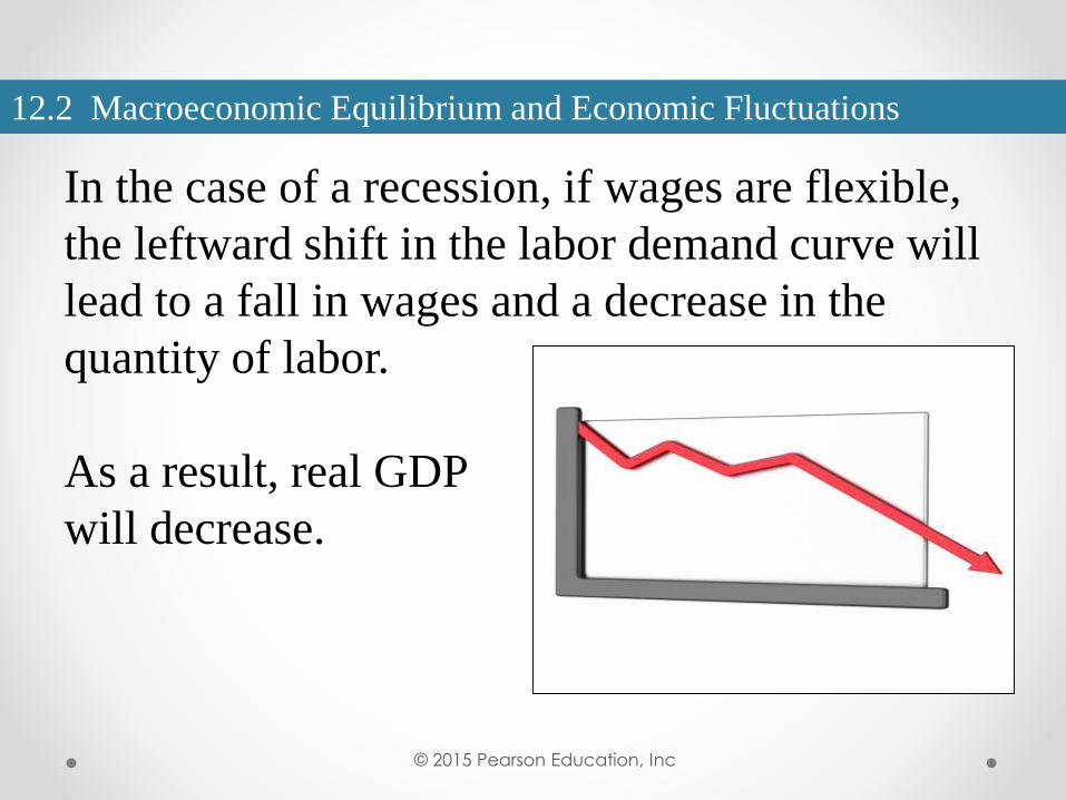
In the case of a recession, if wages are flexible,
the leftward shift in the labor demand curve will
lead to a fall in wages and a decrease in the
quantity of labor.
As a result, real GDP
will decrease.
© 2015 Pearson Education, Inc
12.2 Macroeconomic Equilibrium and Economic Fluctuations

© 2015 Pearson Education, Inc
12.2 Macroeconomic Equilibrium and Economic Fluctuations
Exhibit 12.6, Panel (a) Leftward Shift in
the Labor Demand Curve with Flexible
Wages
Exhibit 12.6, Panel (b) The Relationship
Between Employment and Real GDP

If wages are downward rigid, the leftward shift in
the labor demand curve will lead to no change in
the wage rate and a larger decrease in the
quantity of labor.
As a result, output will decrease more under
downward rigid wages than under flexible wages.
© 2015 Pearson Education, Inc
12.2 Macroeconomic Equilibrium and Economic Fluctuations

© 2015 Pearson Education, Inc
12.2 Macroeconomic Equilibrium and Economic Fluctuations
Exhibit 12.6, Panel (c) Leftward shift in
the labor demand curve with downward
rigid wages
Exhibit 12.6, Panel (b) The relationship
between employment and real GDP

There are three different schools of thought on the
sources of economic fluctuations:
1. Real business cycle theory emphasizes
changes in productivity and technology
2. Keynesian theory focuses on business and
consumer expectations of the future.
3. Financial and monetary theory looks at
changes in prices and interest rates.
© 2015 Pearson Education, Inc
12.2 Macroeconomic Equilibrium and Economic Fluctuations

Real business cycle theory emphasizes changes
in productivity and technology:
• Technological advances and other
productivity-enhancing innovation cause
expansions.
• An increase in input prices like oil causes
recessions.
© 2015 Pearson Education, Inc
12.2 Macroeconomic Equilibrium and Economic Fluctuations
Keynesian theory focuses on changes in
expectations of the future:
• Animal spirits are the psychological factors
that lead to changes in business and consumer
mood or sentiment. Animal spirits can lead to
decreases in spending (recessions) or
increases in spending (expansions).
© 2015 Pearson Education, Inc
12.2 Macroeconomic Equilibrium and Economic Fluctuations

Keynesian theory (cont’d):
• A negative shock can hit the economy and
generate pessimism. Willingness to spend
decreases and is not offset by increased
spending in other parts of the economy.
© 2015 Pearson Education, Inc
12.2 Macroeconomic Equilibrium and Economic Fluctuations
Keynesian theory (cont’d):
• The initial decrease in spending is amplified
by further decreases in other persons’ spending
due to multipliers.
© 2015 Pearson Education, Inc
12.2 Macroeconomic Equilibrium and Economic Fluctuations

Financial and monetary theory—whose main
proponent is Milton Friedman—looks at changes
in prices and interest rates:
• A decrease in the money supply (M2) will
cause the price level to fall.
• A fall in the price level will reduce
employment because of downward wage
rigidity.© 2015 Pearson Education, Inc
12.2 Macroeconomic Equilibrium and Economic Fluctuations

Financial and monetary theory (cont’d):
• A decrease in the money supply (M2) will also
cause an increase in the real interest rate.
• Higher real interest rates will reduce
investment spending by firms.
© 2015 Pearson Education, Inc
12.2 Macroeconomic Equilibrium and Economic Fluctuations

Multipliers can amplify
the effects of any
economic shock,
regardless of its source.
Consider a negative
consumption shock.
© 2015 Pearson Education, Inc
12.2 Macroeconomic Equilibrium and Economic Fluctuations

© 2015 Pearson Education, Inc
12.2 Macroeconomic Equilibrium and Economic Fluctuations
Exhibit 12.8 Multipliers in a Contracting Economy

By lowering household income, multipliers will
shift the labor demand curve further to the left.
As a result, wages and employment will decrease
further, to the trough of the business cycle.
© 2015 Pearson Education, Inc
12.2 Macroeconomic Equilibrium and Economic Fluctuations

© 2015 Pearson Education, Inc
12.2 Macroeconomic Equilibrium and Economic Fluctuations
Exhibit 12.9 Multipliers in an Economy with Flexible Wages
In addition, multipliers can reduce labor demand
further by:
© 2015 Pearson Education, Inc
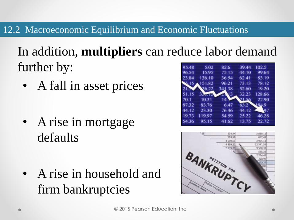
12.2 Macroeconomic Equilibrium and Economic Fluctuations
• A fall in asset prices
• A rise in mortgage
defaults
• A rise in household and
firm bankruptcies
Here is how a shock plays out in the short run:
1. An initial shock shifts the labor demand curve
to the left.
2. Downward wage rigidity leads to greater
reductions.
3. Multipliers cause the labor demand curve to
shift leftward even more.
© 2015 Pearson Education, Inc
12.2 Macroeconomic Equilibrium and Economic Fluctuations

© 2015 Pearson Education, Inc
12.2 Macroeconomic Equilibrium and Economic Fluctuations
Exhibit 12.11 Multipliers in an Economy with Rigid Wages

Economic recovery in the medium run:
1. Market forces from (a) inventory rebuilding,
(b) technological advances, and (c) financial
intermediation shift the labor demand curve to
the right for a partial recovery.
© 2015 Pearson Education, Inc
12.2 Macroeconomic Equilibrium and Economic Fluctuations

© 2015 Pearson Education, Inc
12.2 Macroeconomic Equilibrium and Economic Fluctuations
Exhibit 12.12 Partial Recovery Due to a Partial Rightward Shift in
the Labor Demand Curve
Economic recovery in the medium run:
2. Expansionary monetary policy will lower
interest rates and raise inflation.
Lower interest rates will raise spending, which
shifts the labor demand curve to the right.
Higher inflation will lower real wages, which
shifts the labor supply curve to the left.
© 2015 Pearson Education, Inc
12.2 Macroeconomic Equilibrium and Economic Fluctuations

© 2015 Pearson Education, Inc
12.2 Macroeconomic Equilibrium and Economic Fluctuations
Exhibit 12.13, Panel (a) The Effect of Inflation on the Labor
Market Equilibrium

Note that the leftward shift in labor supply has an
impact only if the new market-clearing wage is
above the original wage rate.
© 2015 Pearson Education, Inc
12.2 Macroeconomic Equilibrium and Economic Fluctuations

© 2015 Pearson Education, Inc
12.2 Macroeconomic Equilibrium and Economic Fluctuations
Exhibit 12.13, Panel (b) The Effect of Inflation on the Labor
Market Equilibrium
The following diagram puts all these effects
together:
1. Pre-recession starting at point 1 to…
2. Recessionary trough at point 2 to…
3. Partial recovery at point 3 to…
4. Full recovery at point 4
© 2015 Pearson Education, Inc
12.2 Macroeconomic Equilibrium and Economic Fluctuations

© 2015 Pearson Education, Inc
12.2 Macroeconomic Equilibrium and Economic Fluctuations
Exhibit 12.14 Full Recovery
12.3 Modeling Expansions
The focus so far has centered on recessions. We
now shift to economic expansions.
Suppose that Apple and other technology firms
become optimistic about the future demand for
their products.
Question: What happens to its demand for labor?
© 2015 Pearson Education, Inc

12.3 Modeling Expansions
© 2015 Pearson Education, Inc
Exhibit 12.15 Rightward Shift in the Labor Demand Curve, Shift from 1 to 2
Only
12.3 Modeling Expansions
In response, firms that supply the technology get
higher sales, and consumers start to spend more.
Question: What happens in the labor market?
© 2015 Pearson Education, Inc

12.3 Modeling Expansions
© 2015 Pearson Education, Inc
Exhibit 12.15 Rightward Shift in the Labor Demand Curve

Evidence-Based Economics Example:
Question: What caused the recession of 2007–
2009?
Data: Historical data on housing prices (Case-
Shiller home price index), residential
investment (NIPA), foreclosure rates (Mortgage
Bankers’ Association), and bank balance sheets
(FDIC and Lehman Brothers).© 2015 Pearson Education, Inc
12 Short-Run Fluctuations

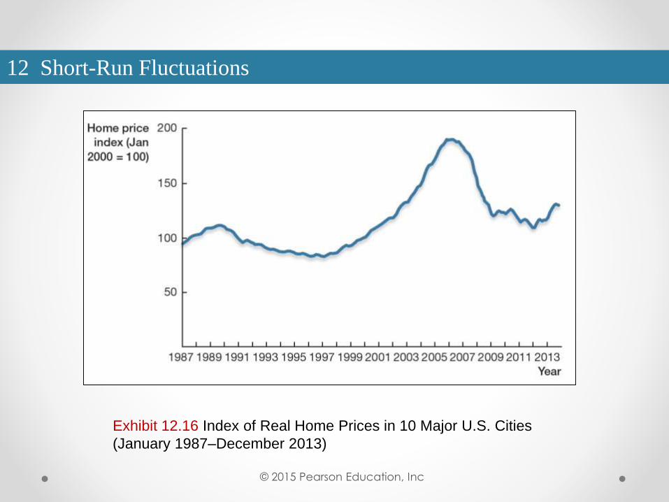
Answer: Three key factors appear to have played
central roles in the crisis:
1. A fall in housing prices, which caused a
collapse in new construction
© 2015 Pearson Education, Inc
12 Short-Run Fluctuations
© 2015 Pearson Education, Inc
Exhibit 12.16 Index of Real Home Prices in 10 Major U.S. Cities
(January 1987–December 2013)
12 Short-Run Fluctuations

© 2015 Pearson Education, Inc
Exhibit 12.17 Real Investment in Residential Construction
(1987:Q1–2013:Q4; Normalized to 100 in 2009)
12 Short-Run Fluctuations
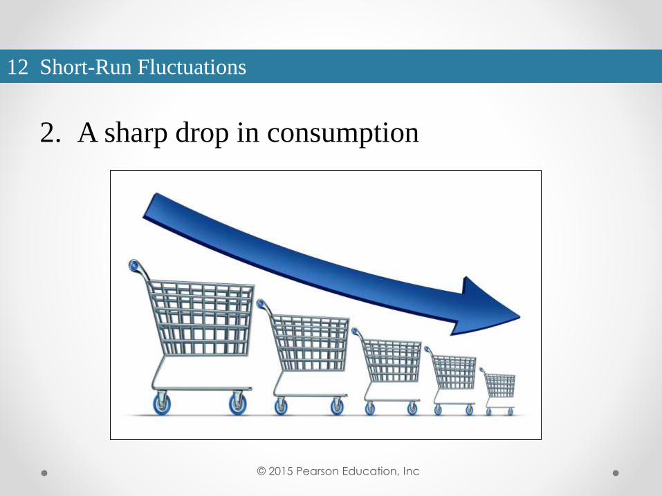
2. A sharp drop in consumption
© 2015 Pearson Education, Inc
12 Short-Run Fluctuations
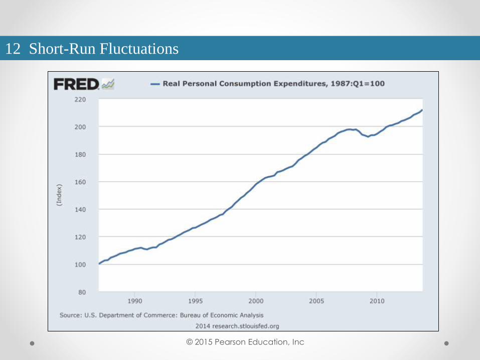
© 2015 Pearson Education, Inc
12 Short-Run Fluctuations

3. Spiraling mortgage defaults that caused many
bank failures, leading the entire financial
system to freeze up
© 2015 Pearson Education, Inc
12 Short-Run Fluctuations
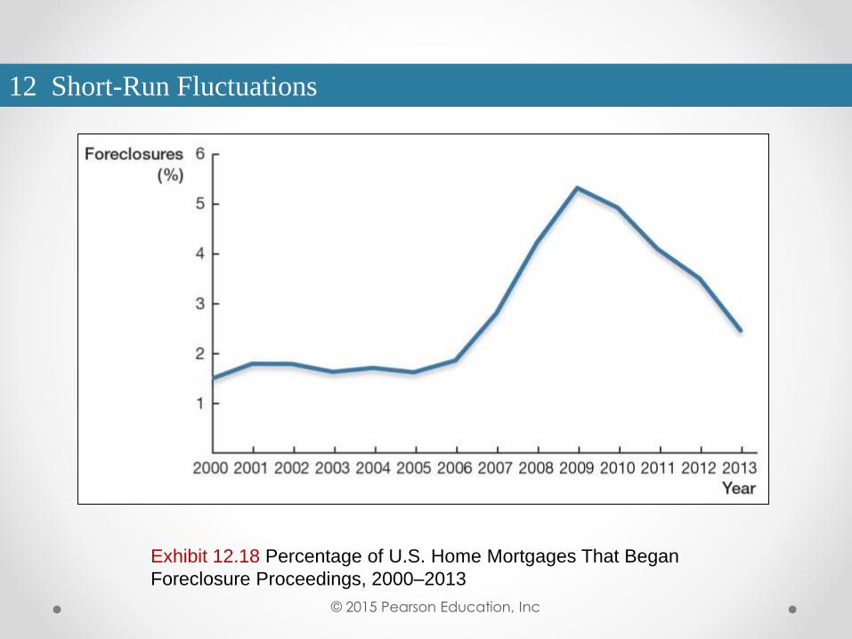
© 2015 Pearson Education, Inc
12 Short-Run Fluctuations
Exhibit 12.18 Percentage of U.S. Home Mortgages That Began
Foreclosure Proceedings, 2000–2013