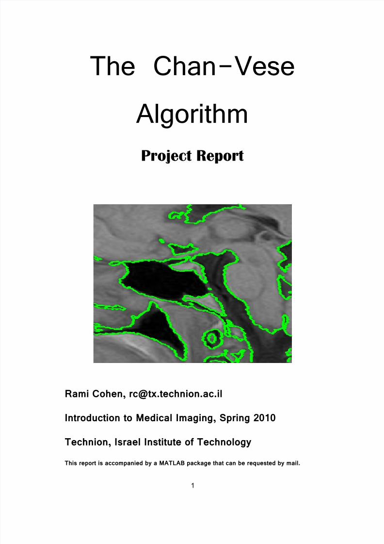
chan vese algorithm

7/27/2019 Chan Vese Algorithm

http://slidepdf.com/reader/full/chan-vese-algorithm 1/18

The Chan-Vese

Algorithm

Project Report

Rami Cohen, [email protected]

Introduction to Medical Imaging, Spring 2010

Technion, Israel Institute of Technology

This report is accompanied by a MATLAB package that can be requested by mail.



2

Table of Contents

1. Introduction ........................................................................................3

2. The model.......................................................................................... 4

3. Level Set formulation ...........................................................................5

4. Numerical scheme ...............................................................................9

4.1 Reinitialization of ........................................................ 11

4.2 Summary of the algorithm 21................................................

5. Code..... ............................................................................................13

6. Results..............................................................................................14

7. Conclusions .......................................................................................16

8. Bibliography ......................................................................................17

9.

Appendix..........................................................................................

18

9.1 Table of equations ........................................................... 18

9.2 Table of figures 2................................................................



3

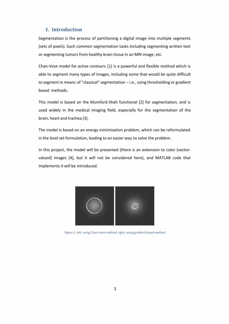
1. Introduction

Segmentation is the process of partitioning a digital image into multiple segments

(sets of pixels). Such common segmentation tasks including segmenting written text

or segmenting tumors from healthy brain tissue in an MRI image, etc.

Chan-Vese model for active contours [1] is a powerful and flexible method which is

able to segment many types of images, including some that would be quite difficult

to segment in means of "classical" segmentation – i.e., using thresholding or gradient

based methods.

This model is based on the Mumford-Shah functional [2] for segmentation, and is

used widely in the medical imaging field, especially for the segmentation of the

brain, heart and trachea [3].

The model is based on an energy minimization problem, which can be reformulated

in the level set formulation, leading to an easier way to solve the problem.

In this project, the model will be presented (there is an extension to color (vector-

valued) images [4], but it will not be considered here), and MATLAB code that

implements it will be introduced.

Figure 1: left: using Chan-Vese method, right: using gradient based method



4

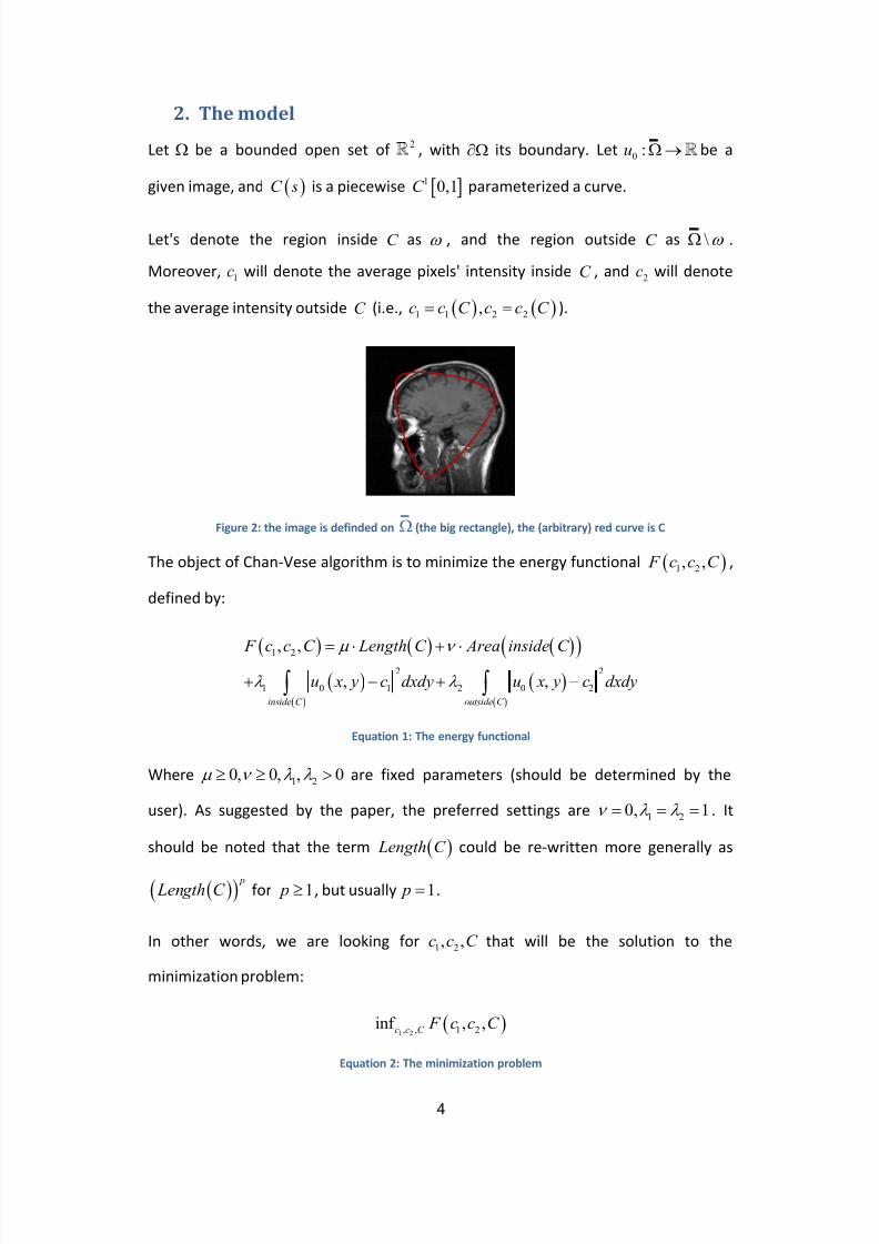
2. The model

Let be a bounded open set of 2

, with its boundary. Let0

:u be a

given image, and C s is a piecewise 1 0,1C parameterized a curve.

Let's denote the region inside C as , and the region outside C as \ .

Moreover,1

c will denote the average pixels' intensity inside C , and2

c will denote

the average intensity outside C (i.e., 1 1 2 2,c c C c c C ).

Figure 2: the image is definded on (the big rectangle), the (arbitrary) red curve is C

The object of Chan-Vese algorithm is to minimize the energy functional 1 2, , F c c C ,

defined by:

1 2

2 2

1 0 1 2 0 2

, ,

, ,inside C outside C

F c c C Length C Area inside C

u x y c dxdy u x y c dxdy

Equation 1: The energy functional

Where 1 20, 0, , 0 are fixed parameters (should be determined by the

user). As suggested by the paper, the preferred settings are 1 20, 1 . It

should be noted that the term Length C could be re-written more generally as

p

Length C for 1 p , but usually 1 p .

In other words, we are looking for 1 2, ,c c C that will be the solution to the

minimization problem:

1 2, , 1 2

inf , ,c c C

F c c C

Equation 2: The minimization problem



5

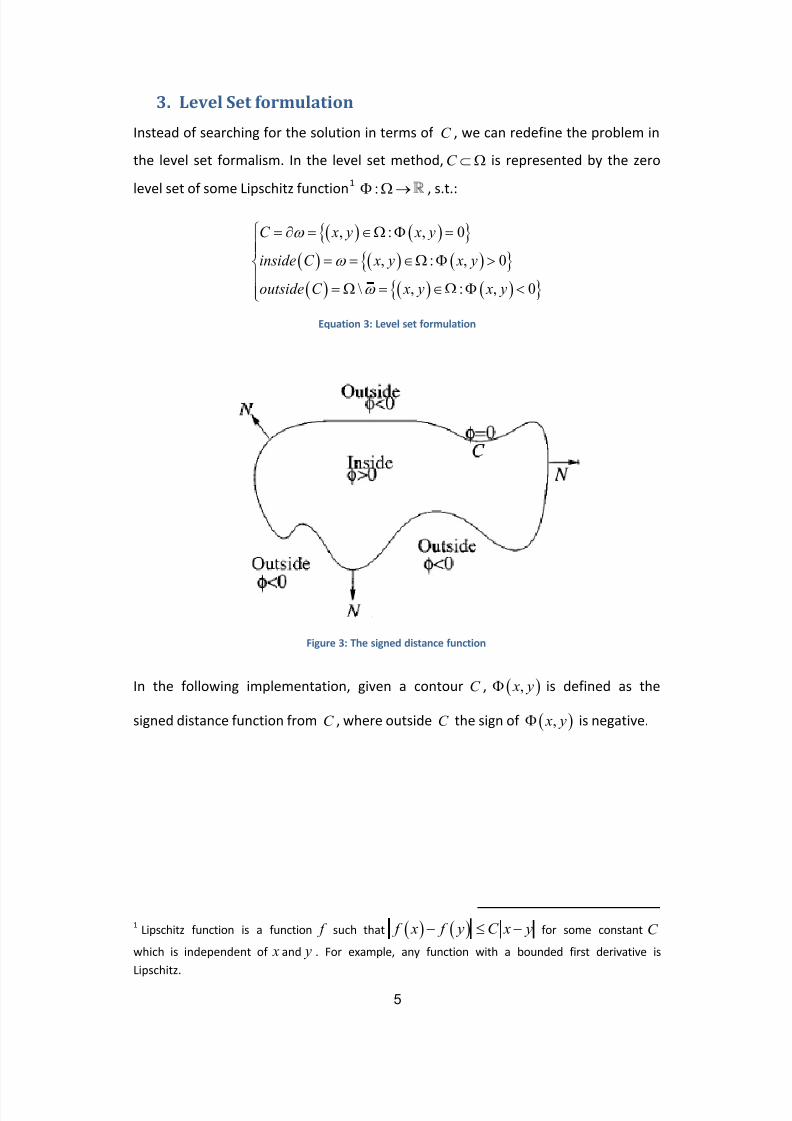
3. Level Set formulation

Instead of searching for the solution in terms of C , we can redefine the problem in

the level set formalism. In the level set method, C is represented by the zero

level set of some Lipschitz function1

: , s.t.:

, : , 0

, : , 0

\ , : , 0

C x y x y

inside C x y x y

outside C x y x y

Equation 3: Level set formulation

In the following implementation, given a contour C , , x y is defined as the

signed distance function from C , where outside C the sign of , x y is negative.

1 Lipschitz function is a function f such that f x f y C x y for some constant C

which is independent of x and y . For example, any function with a bounded first derivative is

Lipschitz.

Figure 3: The signed distance function



6

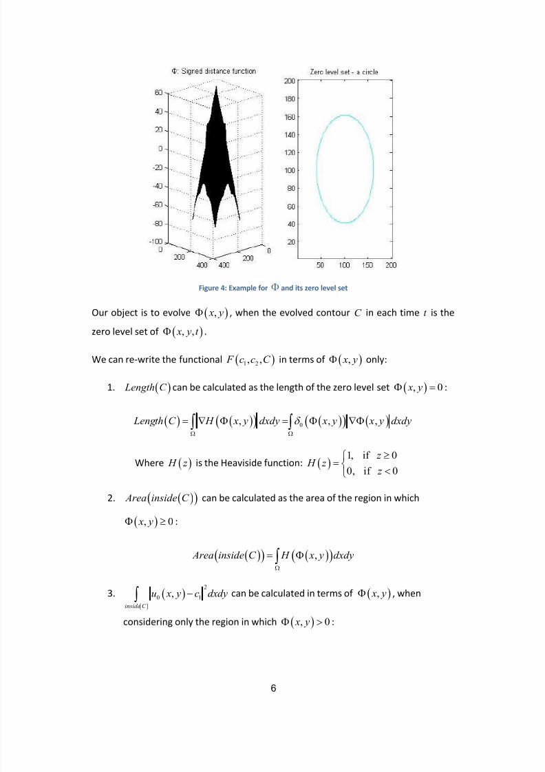
Figure 4: Example for and its zero level set

Our object is to evolve , x y , when the evolved contour C in each time t is the

zero level set of , , x y t .

We can re-write the functional 1 2, , F c c C in terms of , x y only:

1. Length C can be calculated as the length of the zero level set , 0 x y :

0, , , Length C H x y dxdy x y x y dxdy

Where H z is the Heaviside function: 1, if 0

0, if 0

z H z

z

2. Area inside C can be calculated as the area of the region in which

, 0 x y :

, Area inside C H x y dxdy

3.

2

0 1,inside C

u x y c dxdy can be calculated in terms of , x y , when

considering only the region in which , 0 x y :



7

2 2 2

0 1 0 1 0 1

, : , 0

, , , ,inside C x y x y

u x y c dxdy u x y c dxdy u x y c H x y dxdy

4. in a similar way:

2 2 2

0 2 0 2 0 2

, : , 0

, , , 1 ,outside C x y x y

u x y c dxdy u x y c dxdy u x y c H x y dxdy

5. The average intensities:

0

1

, ,

,

u x y H x y dxdy

c

H x y dxdy

,

0

2

, 1 ,

1 ,

u x y H x y dxdy

c

H x y dxdy

The above leads us to the energy functional in terms of 1 2, ,c c (where

1 1 2 2,c c c c and 0 x is Dirac delta function):

1 2 0

2 2

1 0 1 2 0 2

, , , , ,

, , , 1 ,

F c c x y x y dxdy H x y dxdy

u x y c H x y dxdy u x y c H x y dxdy

Equation 4: Energy functional in terms of

Observing the terms in equation 4, we can say that the evolution of the curve is

influenced by two terms ( is usually set to 0, so we will ignore it): the curvature

regularizes the curve and makes it smooth during evolution; the "region term"

2 2

1 0 1 2 0 2u c u c affects the motion of the curve [5].

The term 0, , x y x y dxdy

is the penalty on the total length of the

curve C . For example, if the boundaries of the image are quite smooth, we will give

a larger value, to prevent C from being a complex curve.

1 2, affect the desired uniformity inside C and outside C , respectively. For

example, It would be advisable to set 1 2 when we expect an image with quite

uniform background and varying grayscale objects in the foreground.



8

Using Euler-Lagrange equations and the gradient-descent method, it is shown in the

paper that , x y which minimizes the energy 1 2, , F c c satisfies the PDE ( t is an

artificial time):

1

2 2

1 0 1 2 0 2

1

2 2

1 0 1 2 0 2

dxdy div

dxdy

, ,0 , , 0 on

p

p

o

p u c u ct

p u c u c

x y x yn

Equation 5: PDE for , , x y t

Where is the curvature of the evolving curve (for some specific height level in

). We saw at class that the curvature can be calculated using the spatial

derivatives of up to second order:

2 2

3/22 2

2 xx y xy x y yy x

x y

Equation 6: Curvature

Figure 5: Curvature at a point can tell how fast the curvature is turning there



9

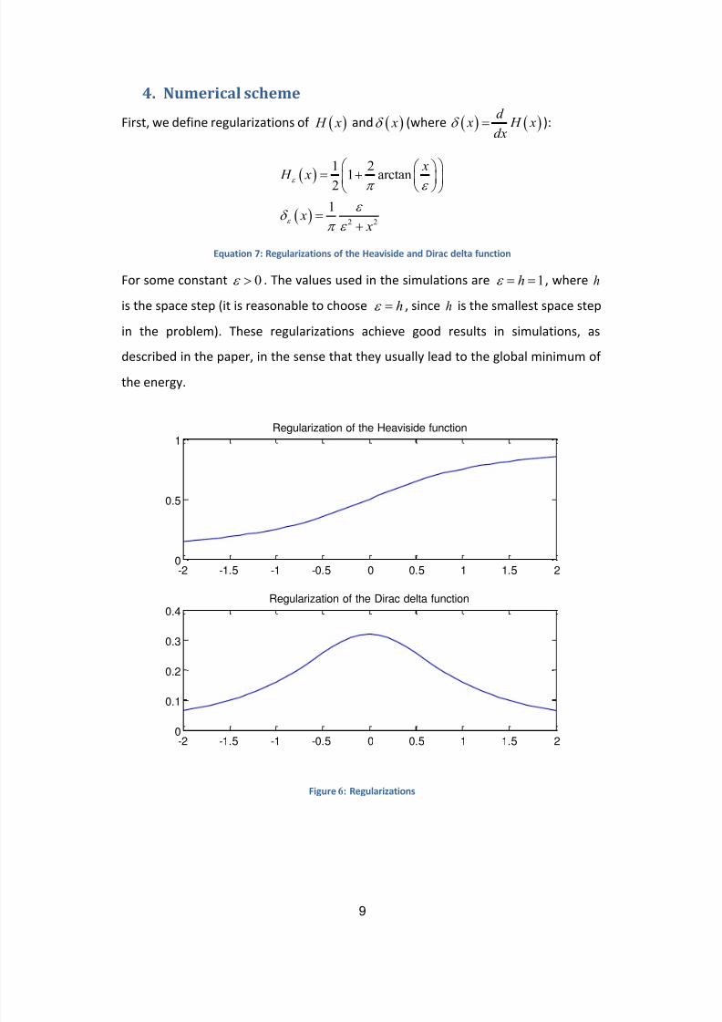
4. Numerical scheme

First, we define regularizations of H x and x (where d

x H xdx

):

2 2

1 21 arctan2

1

x H x

x x

Equation 7: Regularizations of the Heaviside and Dirac delta function

For some constant 0 . The values used in the simulations are 1h , where h

is the space step (it is reasonable to choose h , since h is the smallest space step

in the problem). These regularizations achieve good results in simulations, as

described in the paper, in the sense that they usually lead to the global minimum of

the energy.

Figure 6: Regularizations

-2 -1.5 -1 -0.5 0 0.5 1 1.5 20

0.5

1Regularization of the Heaviside function

-2 -1.5 -1 -0.5 0 0.5 1 1.5 20

0.1

0.2

0.3

0.4Regularization of the Dirac delta function



1

Let's define , , ,n

i j i jn t x y where t is the time step. The PDE can be

discretisized by using the following notations for spatial finite differences (where

x yh h h ):

, , 1, , 1, ,

, , , 1 , , 1 ,

/ , /

/ , /

x n n n x n n n

i j i j i j i j i j i j

y n n n y n n n

i j i j i j i j i j i j

h h

h h

The linearized, discretized PDE becomes:

, ,

,

2 2 22

1 , , 1 , 1, ,

, 2

,

2 2 22

, 1, 1, 1

2 2

, 1 1 2 2

/ / 2

/ / 2

i j i j

x n

i j x

x n n n

n n i j i j i ji j i j n

h i j

y n

i j y

y n n n

i j i j i j

n n n

h i j o o

h h

t h

h h

u c u c

Equation 8: The linearized, discretized PDE

Defining the following constants (for a given

n):

1 2

2 2 2 2

1, , , 1 , 1 , 1, 1, 1, 1

1 1,

/ 4 / 4n n n n n n n n

i j i j i j i j i j i j i j i j

C C

3 4

2 2 2 2

1, 1, , 1 , 1, 1 1, 1 , , 1

1 1,

/ 4 / 4n n n n n n n n

i j i j i j i j i j i j i j i j

C C

We get the simplified equation:

, ,

11

, , 1 2 3 4

1

, , 1 1, 2 1, 3 , 1 4 , 1

2 2

, 1 0 1 2 0 2

1

i j i j

pn n n

i j h i j

pn n n n n n n

i j h i j i j i j i j i j

n n n

h i j

t p L C C C C

h

t p L C C C C

h

t u c u c

Equation 9: Simplified PDE



Where we calculate 1 2,n n

c c as discretized sums, using the regularized

Heaviside function. In addition, n L is Length C as was calculated at section 3.

As suggested in the paper, in order to solve equation 10, we can use an iterative

way, as pointed out by [6], proposition 6.1, in which it is also proved that there exists

a solution to the equation.

4.1 Reinitialization of

In each step, we need to reinitialize , x y to be the signed distance function to its

zero level set. This procedure prevents the level set function from becoming too

"flat", an effect which is caused due the use of the regularized delta function x ,

which causes blurring.

The reinitialization process is made by using the following PDE:

, , 1

0 , ,

sign x y t

x y t

Equation 10: Reinitialization

The solution of this equation, , will have the same zero level set as , , x y t , and

away from this level set, will converge to 1, as it should be for a distance

function.

The numerical equation for equation 11:

1

, , ,, ,n n n

i j i j i j sign x y t G

Equation 11: Numerical scheme for reinitialization

Where the "flux" ,

n

i jG is defined using the notations , , ,a b c d , defined by:



2

, , 1,

, 1, ,

, , , 1

, , 1 ,

/ /

/ /

/ /

/ /

x

i j i j i j

x

i j i j i j

y

i j i j i j

yi j i j i j

a h h

b h h

c h h

d h h

and

2 2 2 2

2 2 2 2

,

max , max , 1, , , 0

max , max , 1, , , 0

0,

i j

n

i j i j

a b c d x y t

G a b c d x y t

otherwise

Equation 12: definition of G

where max ,0 , min ,0a a a a and so on.

4.2 Summary of the algorithm

1. Initialize 0

,

n

i j

to some Lipschitz function0

2. Compute 1 2,n n

c c

3. Solve the PDE of equation 9

4. Reinitialize 1

,

n

i j

to be the signed distance function to 1

, 0n

i j

by using

equation 11

5. Check whether the solution is stationary. If not, continue. Else, stop.

In practice, the process should be stopped when,

1 2

, ,ni j

n n

i j i jhQ t h

(this should be checked at stage no. 5) where M is the number of grid points which

satisfy ,i j h , because , , x y t is not expected to change anymore (except for

maybe some small numerical changes).



3

5. Code

The numerical scheme above was implemented using MATLAB. The attached source

files are (more documentation can be found in the source code):

1. CV.m – the main file.

2. delta.m – regularized Dirac delta function (equation 7).

3. heaviside.m - regularized Heaviside function (equation 7).

4. reinit.m – reinitialization of 1

,

n

i j

by the method proposed at 4.1.

5. cur_diff – checking whether,

n

i j reached its steady state according to the

method proposed at 4.2

The input images should be grayscale only; otherwise they will be converted into

grayscale. Moreover, there is an option to select only a (rectangular) part of the

image, and the segmentation process will be applied only to this part. It can come in

handy when the image is large and we want to segment just a part of it.

As always, larger images need more computational time. It is highly recommended

to use images of a small size (i.e., no more than 256x256 pixels), and to not stop the

segmentation process before it ends (in other words, don't use ctrl+c). In weak

computers it can cause some instability.



4

6. Results

The first example is similar to the example which appears at the paper – an image

with (approx.) only two gray levels.

As can be seen from figure, a good segmentation was achieved.

Let's see how it segments an MRI image (resized):

Since Chan-Vese algorithm is not based on gradient methods, it achieves good results even

when the image is blurred:

Figure 7: left: clear objects, right: segmentation

Figure 8: left: MRI image, right: segmentation

Figure 9: left: blurred objects, right: segmentation



5

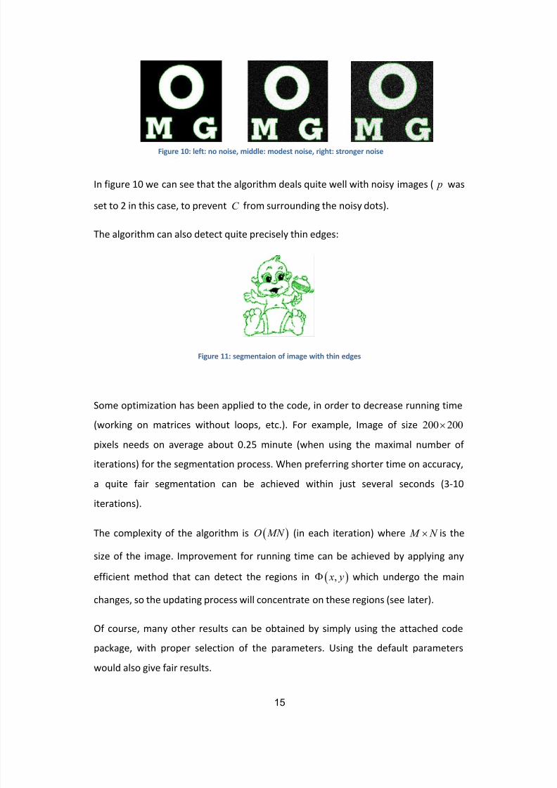
In figure 10 we can see that the algorithm deals quite well with noisy images ( p was

set to 2 in this case, to prevent C from surrounding the noisy dots).

The algorithm can also detect quite precisely thin edges:

Figure 11: segmentaion of image with thin edges

Some optimization has been applied to the code, in order to decrease running time

(working on matrices without loops, etc.). For example, Image of size 200 200

pixels needs on average about 0.25 minute (when using the maximal number of

iterations) for the segmentation process. When preferring shorter time on accuracy,

a quite fair segmentation can be achieved within just several seconds (3-10

iterations).

The complexity of the algorithm is O MN (in each iteration) where M N is the

size of the image. Improvement for running time can be achieved by applying any

efficient method that can detect the regions in , x y which undergo the main

changes, so the updating process will concentrate on these regions (see later).

Of course, many other results can be obtained by simply using the attached code

package, with proper selection of the parameters. Using the default parameters

would also give fair results.

Figure 10: left: no noise, middle: modest noise, right: stronger noise



6

7. Conclusions

Chan-Vese algorithm was implemented in this project. From the results above, it can

be seen that this algorithm deals quite well even with images which are quite

difficult to segment in the regular methods, such as gradient-based methods or

thresholding.

This can be explained by the fact that CV algorithm relies on global properties

(intensities, region areas), rather than just taking into account local properties, such

as gradients. One of the main advantages of this approach is better robustness for

noise, for example.

As mentioned before, the algorithm is sometimes quite slow, especially when

dealing with large images. It can pose a problem for real time applications, such as

video sequences, and an efficient implementation is very important.

There are some papers which suggest refinements to this algorithm, especially for

the time-consuming computation of the PDE solution. These methods use values

that were already computed, in order to decrease the computing time of the next

values. Such approaches can be found in [5], [7] .

CV algorithm is a very powerful algorithm, as we have also seen in the results above.

This algorithm marks some "modern" approach for image segmentation, which relies

on calculus and partial differential equations.



7

8. Bibliography

[1] T. Chan and L. Vese, "Active contours without edges," in IEEE transactions on image

processing 10(2), 2001, pp. 266-277.

[2] D. Mumford and J. Shah, "Optimal approximation by piecewise smooth functions andassociated variational problems," Comm. Pure Appl. Math, vol. 42, pp. 577-685, 1989.

[3] Olivier Rousseau and Yves Bourgault, "Heart segmentation with an iterative Chan-Vese

algorithm," University of Ottawa, Ontario , 2009.

[4] Chan et. al, "Active Contours without Edges for Vector-Valued Images," Journal of Visual

Communication and Image Representation, vol. 11, pp. 130-141, 2000.

[5] Pan et. al, "Efficient Implementation of the Chan-Vese Models Without Solving PDEs," in

International Workshop On Multimedia Signal Processing, 2006, pp. 350-353.

[6] G. Aubert and L. Vese, "A variational method in image recovery," SIAM J. Num. Anal., vol.

34/5, pp. 1948-1979, 1997.

[7] Zygmunt L. szpak and Jules R. Tapamo, "Further optimization for the Chan-Vese active

contour model," in High perfomance computing & simulation conference, 2008.



8

9. Appendix

9.1 Table of equations

Equation 1: The energy functional..................................................................................

4

Equation 2: The minimization problem............................................................................4

Equation 3: Level set formulation ...................................................................................5

Equation 4: Energy functional in terms of ...................................................................7

Equation 5: PDE for , , x y t ......................................................................................8

Equation 6: Curvature ...................................................................................................8

Equation 7: Regularizations of the Heaviside and Dirac delta function ................................9

Equation 8: The linearized, discretized PDE ....................................................................10

Equation 9: Simplified PDE ...........................................................................................10

Equation 10: Reinitialization.........................................................................................

11

Equation 11: Numerical scheme for reinitialization .........................................................11

Equation 12: definition of G .......................................................................................12

9.2 Table of figures

Figure 1: left: using Chan-Vese method, right: using gradient based method .......................3

Figure 2: the image is definded on (the big rectangle), the (arbitrary) red curve is C .........4

Figure 3: The signed distance function ............................................................................5

Figure 4: Example for and its zero level set ..................................................................6

Figure 5: Curvature at a point can tell how fast the curvature is turning there.....................

8

Figure 6: Regularizations................................................................................................9

Figure 7: left: clear objects, right: segmentation .............................................................14

Figure 8: left: MRI image, right: segmentation................................................................14

Figure 9: left: blurred objects, right: segmentation .........................................................14

Figure 10: left: no noise, middle: modest noise, right: stronger noise................................15

Figure 11: segmentaion of image with thin edges ...........................................................15

http://c/Users/Rami/Desktop/project%20chan%20vese/chan_vese.docx%23_Toc267615688

























chan vese algorithm

Documents