change-point detectionon swing funds · change-point detection on swing funds ... divisive and...
TRANSCRIPT

University of Amsterdam
MSc in Stochastics and
Financial Mathematics
Master Thesis
Change-Point Detectionon Swing Funds
Examiner:
Dr. A.J. van Es
Supervisor:
Dr. Jan Jaap Hazenberg
Author:
Lin Lou
August 28, 2014


I would like to dedicate this thesis to my loving parents.


Acknowledgements
Foremost, I would like to thank my supervisor Dr. A.J.(Bert) van Es for his patience,motivation, humor, and knowledge. He is also the person that recruited me to this Masterprogram. To some extent he helped me fulfil a dream of mine. Two years ago, I was won-dering whether I should go to work or try to study something I always wanted to. Afterthe submission of this thesis, I can say that I left no regrets in my school days. Without hisguidance in all the time of research and writing, this thesis cannot be done.
Besides my supervisor, I would also like to express my sincere gratitude to Dr. Jan JaapHazenberg who offered me the excellent internship opportunity. He led me to a new andchallenging research subject. During the time I worked for him, I learned quite a lot fromhim and his team. His professional experience also helped me crack many research ques-tions and inspired me to develop the methodologies.
I also want to thank Willem van der Scheer, Wilmar Langerak and Ilya Kulyatin, threeformer colleagues of mine, for the stimulating discussions on the paper and methodologies,for the days we were working together, and for the trust they had on me.
Last but not the least, I would like to thank my parents. My love for them cannot be ex-pressed in words.


Abstract
In this thesis we develop a method to find the threshold of trading volume in swing pric-ing policy. This method is based on the simulation of market excess returns given differentvalues of thresholds. The best estimate of the swing pricing threshold is the one that fits theswing pricing pattern the most. Since a fund management company may change its swingpricing policy, our study also means to find what change-point detection methods in multi-variate observations are more suitable for our research porpoise. Empirically, we find thatthe Bai-Perron break point analysis can give us satisfactory results. We aim to see whetherthere are alternative methods that can outperform the Bai-Perron. The latest nonparamet-ric change-point detection method developed by Matteson and James (2013) is based ondivisive and agglomerative clustering, which can also work for multivariate distributions.Combined with our threshold detection model, we do not find that the two new methods cancertainly improve the results.

Contents
Contents vi
List of Figures viii
List of Tables ix
Nomenclature ix
1 Introduction 11.1 Anti-Dilution . . . . . . . . . . . . . . . . . . . . . . . . . . . . . . . . . 1
1.2 Change-Point Analysis . . . . . . . . . . . . . . . . . . . . . . . . . . . . 3
2 Swing Pricing 62.1 Determining the Threshold within Fixed Regime Time Interval . . . . . . . 6
2.2 Estimating Change Points of Swing Regimes . . . . . . . . . . . . . . . . 10
2.3 Test Statistics . . . . . . . . . . . . . . . . . . . . . . . . . . . . . . . . . 12
3 Hierarchical Change Point Analysis 153.1 General Framework . . . . . . . . . . . . . . . . . . . . . . . . . . . . . . 15
3.2 Agglomerative Clustering . . . . . . . . . . . . . . . . . . . . . . . . . . . 16
3.2.1 Divergence in Multivariate Distributions . . . . . . . . . . . . . . . 16
3.2.2 Merging . . . . . . . . . . . . . . . . . . . . . . . . . . . . . . . . 19
3.3 Change Point Estimation . . . . . . . . . . . . . . . . . . . . . . . . . . . 23
3.3.1 Estimating the Locations of Change Points . . . . . . . . . . . . . 23
3.3.2 Hierarchical Estimating Methods . . . . . . . . . . . . . . . . . . 24
3.3.3 Significance Testing . . . . . . . . . . . . . . . . . . . . . . . . . 27
3.4 Time Series Analysis . . . . . . . . . . . . . . . . . . . . . . . . . . . . . 28

Contents vii
4 Simulation 304.1 Independent Sequences . . . . . . . . . . . . . . . . . . . . . . . . . . . . 304.2 Autocorrelated Sequence . . . . . . . . . . . . . . . . . . . . . . . . . . . 32
5 Empirical Results 385.1 Data Description . . . . . . . . . . . . . . . . . . . . . . . . . . . . . . . 385.2 Empirical Threshold and Change Points . . . . . . . . . . . . . . . . . . . 42
6 Conclusion 47
Bibliography 49
Appendix A Change-Point Detection Algorithm 51A.1 E-Divisive Algorithm . . . . . . . . . . . . . . . . . . . . . . . . . . . . . 51A.2 E-Agglomerative Algorithm . . . . . . . . . . . . . . . . . . . . . . . . . 52
Appendix B Some Matlab Codes 53B.1 Threshold Finder Model . . . . . . . . . . . . . . . . . . . . . . . . . . . 53B.2 The E-Divisive Distance . . . . . . . . . . . . . . . . . . . . . . . . . . . 56

List of Figures
3.1 22 Public Utilities . . . . . . . . . . . . . . . . . . . . . . . . . . . . . . . 213.2 Ward’s Clustering . . . . . . . . . . . . . . . . . . . . . . . . . . . . . . . 223.3 e-distance alpha=1 . . . . . . . . . . . . . . . . . . . . . . . . . . . . . . 223.4 Euclidean Clustering . . . . . . . . . . . . . . . . . . . . . . . . . . . . . 233.5 E-Divisive Algorithm . . . . . . . . . . . . . . . . . . . . . . . . . . . . . 253.6 E-Agglomerative Algorithm . . . . . . . . . . . . . . . . . . . . . . . . . 26
4.1 Change in a Univariate Gaussian Sequence . . . . . . . . . . . . . . . . . . 314.2 Changes in Correlation and Paremeters . . . . . . . . . . . . . . . . . . . . 354.3 Only Correlation Change . . . . . . . . . . . . . . . . . . . . . . . . . . . 36
5.1 Correlogram of JPM . . . . . . . . . . . . . . . . . . . . . . . . . . . . . 405.2 Correlogram of CS . . . . . . . . . . . . . . . . . . . . . . . . . . . . . . 415.3 Correlogram of Natixis . . . . . . . . . . . . . . . . . . . . . . . . . . . . 415.4 Market Excess Returns of Natixis . . . . . . . . . . . . . . . . . . . . . . 445.5 Flow Percentage of Natixis . . . . . . . . . . . . . . . . . . . . . . . . . . 44

List of Tables
2.1 General Swing Pattern . . . . . . . . . . . . . . . . . . . . . . . . . . . . 8
4.1 Deteced Change Points in Simulatied VAR(1) . . . . . . . . . . . . . . . . 354.2 Detected Correlation Change in Simulatied VAR(1) . . . . . . . . . . . . . 37
5.1 Fund Info . . . . . . . . . . . . . . . . . . . . . . . . . . . . . . . . . . . 395.2 Sample Market Excess Returns . . . . . . . . . . . . . . . . . . . . . . . . 395.3 Sample Flow Percentage . . . . . . . . . . . . . . . . . . . . . . . . . . . 405.4 Thresholds Detected without Change Point Study . . . . . . . . . . . . . . 425.5 Detected Change Points (Bai and Perron) . . . . . . . . . . . . . . . . . . 435.6 Swing Pricing Threshold (Bai and Perron) . . . . . . . . . . . . . . . . . . 435.7 Detected Change Points (E-Divisive) . . . . . . . . . . . . . . . . . . . . . 455.8 Detected Change Points (E-Agglomerative) . . . . . . . . . . . . . . . . . 455.9 Thresholds by Hierarchical Methods . . . . . . . . . . . . . . . . . . . . . 46


Chapter 1
Introduction
This thesis is a part of the study that I conducted in ING Investment Management (INGIM). In this thsis, we develop a unique methodology that allows us to find the swing thresh-old and detect the changes of a fund’s anti-dilution policy, known as swing pricing, fromits daily NAV, number of outstanding shares and benchmark time series. As a continuationof my work in ING IM, we propose alternative methods to detect change points in a fund’sswing pricing policy in order to see if there is a better alternative to our model. In the em-pirical part of the thesis, we test the methodology on a sample of high yield bond funds.This category has relatively high transactions costs in underlying portfolios, resulting in afavorable signal-to-noise ratio.
1.1 Anti-Dilution
The first open-end fund worldwide, The Massachusetts Investors’ Trust, was launchedin the United States (U.S.) in 1924 (Wilcox, 2003, p. 645) [29]. After a relatively slowstart, this fund would become the largest U.S. investment fund in the 1950s. The open-endconcept was copied by other funds in the U.S. already from the 1920s and in other countriesafter World War II (Slot, 2004, p. 107-108) [25] and this fund structure has become thedominant structure for funds globally . Mutual funds in Europe, set-up in accordance withthe UCITS Directive, are obliged to have an open-end structure, providing investors thepossibility to buy or sell units at least twice a month. In practice, substantially all UCITSfunds provide daily liquidity.
An advantage of open-end funds is that investors can always redeem their fund investmentat a price based on the Net Asset Value (NAV). When investors do not like the results of

2 Introduction
the fund in which they are invested, they can sell their investment and effectively fire themanagement company. However, there is a disadvantage associated with the liquidity ofopen-end funds. When the price of a fund on a dealing day is the same for redemptions andsubscriptions and only reflects the value of the net assets of the fund per share, transactioncosts at the portfolio level of the fund incurred as a result of net subscriptions into or netredemptions from the fund fall on all existing investors in the fund, not on the investorstrading that day. The transaction costs in the portfolio as a result of the capital activity atthe level of the fund, dilute the value of existing shareholders’ interests. In effect, the per-formance of the fund is reduced by these transaction costs and wealth is transferred fromexisting investors to investors subscribing or redeeming.
This dilution affect can be mitigated when funds are not traded at NAV, but apply a bid-and-ask price, where the difference between NAV and price accrues to the fund, or useswing pricing. Swing pricing is an approach where there is one transaction price per day,but that price is higher than the NAV when there are net subscriptions and is lower whenthere are net redemptions. This type of anti-dilution measures is not compliant with U.S.fund regulation. In Europe, the UCITS Directive neither obliges, nor forbids funds to im-plement such an anti-dilution policy. This has resulted in different regulations and marketpractice across the various markets within the European Union. In Luxembourg and Ireland,the two largest UCITS domiciles for cross-border fund distribution (Lipper, 2010) [16], it isleft to the discretion of the fund management company as to whether or not any anti-dilutionmeasures are implemented, resulting in differences between fund providers and individualfunds in the anti-dilution policy applied. This ranges from funds not taking any anti-dilutionmeasures to funds applying a full swing policy, whereby the mechanism is applied on eachdealing day that there are subscriptions or redemptions. Others apply partial swing pric-ing, whereby the mechanism is applied only when the total net cash flow exceeds a certainpre-set threshold. The level of the anti-dilution charge, the swing factor, is not standardizedeither.
Both in Luxembourg and Ireland, fund management companies tend to provide only mini-mal transparency with regard to their anti-dilution policy. However, typically fund providersonly publish daily transaction prices, not the NAV before the anti-dilution adjustment or thefactor by which the NAV is adjusted to counter dilution. Also the thresholds applied arenot disclosed with the argument that this would encourage "gaming" of the threshold, i.e.large investors spreading their subscriptions and redemption over multiple days in order not

1.2 Change-Point Analysis 3
the breach the threshold and activate the swing pricing mechanism on any day. For fundinvestors, this obscurity has a number of disadvantages. Firstly, when considering a sub-scription or redemption, an investor does not know whether swing pricing will occur, nor,when it does, by which percentage. Secondly, an investor cannot evaluate the effectivenessof the anti-dilution policy of a fund compared to other funds available. Thirdly, swing pric-ing makes it more difficult to evaluate the performance of a fund. A fund’s performance isdependent on the investments made by the fund - which in turn reflect the skill of the port-folio manager - and of the anti-dilution policy applied. Performance statistics published bya fund and available from sources such as Morningstar are not decomposed in componentsreflecting portfolio performance and the swing pricing policy, respectively. These disad-vantages combined make it difficult for a fund investor to select the appropriate fund forinvestment.
1.2 Change-Point Analysis
Change point analysis is the process of detecting distributional changes within observa-tions . Nowadays, with the growing importance of financial modeling, change point analysisalso has been increasingly applied to the financial industry. In the finance literature, one ofthe most popular empirical techniques for assessing the informational impact of an ’event’is the ubiquitous ’event’ study. This was pioneered by Fama et al. (1969) [8] in a famousstudy of stock splits, and by Ball and Brown (1968) [4] in their analysis of the impact ofchanges in accounting numbers. In our study, we examine the swing pricing events, whichare the co-movements between fund’s returns and fund’s flows.
It is very crucial to know where a swing pricing policy changes. The change in a swingpricing policy does not only refer to the change on the volume of selling and buying, butalso relates to when a swing pricing policy is kicked into a fund. For some funds the swingpricing policy has been introduced years ago. However, there are also some funds thatrecently implement the anti-dilution mechanism. Knowing when the swing policy is intro-duced to a fund is relevant to study the fund management company’s strategy. Moreover,a fund management company may also change its swing policy. Hence, given a fund’s in-formation for a period, if we know when the policy is introduced and when it changes, wecan divide this period into subgroups according to its changes. Afterwards we can study theswing pricing policy in each subperiod to get the whole picture of this fund’s swing pricing

4 Introduction
for the period.
The history of change point analysis can be dated back to sixty years ago. Page (1954)[22] devises CUSUM as a method to determine changes in it, and proposed a criterion fordeciding when to take corrective action. In general, change point analysis may be per-formed in either parametric and nonparametric settings. Parametric analysis necessarilyassumes that the underlying distributions belong to some known family, and the likelihoodfunction plays a major role. For example, in Lange, Carlin et al. (1992) [14] and Lavielleand Teyssiere (2006) [15] analysis is performed by maximizing a log-likelihood function,while Page (1954) examines the ratio of log-likelihood functions to estimate change points.Bai and Perron (1998) [2] consider issues related to multiple structural changes, occurringat unknown dates, in the linear regression model estimated by least squares. Additionally,Davis et al. (2006) [6] combine the log-likelihood, the minimum description length, and agenetic algorithm in order to identify change points. Nonparametric alternatives are appli-cable in a wider range of applications than parametric ones (Hariz et al., 2007) [9]. Erdmanand Emerson (2007) [7] design a method to perform Bayesian single change point analysisof univariate time series. It returns the posterior probability of a change point occurring ateach time index in the series. Nonparametric approaches often rely heavily on the estima-tion of density functions (Kawahara and Sugiyama, 2011) [10], though they have also beenperformed using rank statistics (Lung-Yut-Fong et al., 2011) [17].
Another issue in change point analysis is the dimensionality. Most of methods mentionedin the last paragraph focus on the univariate data. Killick and Eckley (2011) [11] providesmany methods for performing change point analysis of univariate time series. Currently,their method is only suitable for finding changes in mean or variance. Although their methodonly considers the case of independent observations, the theory and application behind theimplemented methods allows for certain types of serial dependence (Killick et al., 2011)[12]. Ross and Adams (2012) [24] similarly provides a variety of methods for performingchange point analysis of univariate time series. These methods range from those to detectchanges in independent Gaussian data to fully nonparametric methods that can detect gen-eral distributional changes.
We will mainly focus on a newly developed change-point detection method for our swingpricing study. Matteson and James (2013) [19] propose a nonparametric approach basedon Euclidean distances between sample observations. It is simple to calculate and avoids

1.2 Change-Point Analysis 5
the difficulties associated with multivariate density estimation. Their method does not re-quire any estimation of density function. The proposed approach is motivated by methodsfrom cluster analysis (Szekely and Rizzo, 2005) [26]. This method is illustrated in Chap-ter 3. Although Matteson and James (2013) [19] relax the assumptions on the underlyingmultivariate distribution to a large extent, they still assume the independency. However, inChapter 4 we will see that serial dependence, which usually happens in time series data,will jeopardize the performance of their method. In Chapter 5, we also see that their methoddoes not outperform Bai-Perron method for the threshold detection on swing funds.
The layout of the thesis is as follows. Chapter 2 explains the effects swing pricing policygives to a fund’s returns and flow percentage which is defined as the percentage ratio of afund’s flow at day t to the fund’s size at the previous day. In this Chapter we also introducesthe method devised by Bai and Perron in 1998 [2]. Their method empirically works for theswing regime changes in practice. In Chapter 3 we aim to examine an alternative for Bai-Perron method for finding swings within a fixed regime period, which is the nonparametricapproach proposed by Matteson and James. This method is based on hierarchial clusteringof the e-distance derived by (Szekely and Rizzo, 2005) [26]. In Chapter 4 we simulate thisnew method to check whether this method works for autocorrelated observations. One cansee the empirical results in Chapter 5. Chapter 6 concludes.

Chapter 2
Swing Pricing
This chapter aims to give a brief introduction of some financial concepts and explain themechanism of swing pricing
2.1 Determining the Threshold within Fixed Regime TimeInterval
Let Rst and Div be the share class 1 return at time t and the daily dividend of the underly-
ing share class. Let N(s) denote the number of shares for share class s. NAV st is the price of
share class s at time t. Note that the fund return is only based on non-hedged share classesin the base currency of the fund, otherwise the benchmark adjusted return would be affectedby currency results. Suppose there are n share classes of non-hedged share classes in a fund,the weight on share class at time t is given by
wst =NAV s
t ×N(s)∑ns=1 NAV s
t ×N(s)(2.1)
To introduce the threshold detection model, we also need to calculate the return for shareclass s in a fund at time t. Define Rs
t as the share class s’s return at time t, (Rit) as daily
fund return for fund i at time t, wst as the weight for share class s at time t, and daily market
1A designation applied to a specified type of security such as common stock or mutual fund units. Com-panies that have more than one class of common stock usually identify a given class with alphabetic markers,such as "Class A" shares and "Class B" shares. Different share classes within the same entity typically conferdifferent rights on their owners.

2.1 Determining the Threshold within Fixed Regime Time Interval 7
excess return εt . The number of share classes in fund i is n, then we have:
Rst =
NAV st +Divs
tNAV s
t−1−1 (2.2)
Rit =
n∑s=1
wstRst (2.3)
By definition, market excess return is defined to be the difference between a fund’s returnsand its underlying benchmark 2 returns. Let Rb
t be the benchmark return at time t, definedby Pt/Pt−1 −1, where Pt is the benchmark’s price at time t. However, in reality funds maybe priced at different times than benchmarks. We have seen multiple funds of which thereturns are highly correlated with benchmark’s returns on the same day and one day before.We can understand this observation since, for example, that the benchmark is priced in theafternoon and the fund is priced at noon. This is probably related to T +1 accounting, whichmeans that funds at day t publish NAVs calculated using t −1 prices based on transactionson t−2. Hence, the fund price will absorb the market information of the current day and theday before. Rb
t−1 is the benchmark return lagged by one day. Hence, we propose to calculatethe market excess return in the following way
Rit = α +β1Rb
t +β2Rbt−1 + εt , (2.4)
where εt is a normal white noise. Also note that the autocorrelation within benchmark’s re-turns barely exists. Hence multicollinearity is not of concern in the above regression model.
For determining potential swing pricing events, the basic idea is that we use that the typicalcharacteristics of a swing pricing pattern. A swing pricing pattern can be characterized bya large market excess return (due to the price adjustment of the fund in order to avoid dilu-tion) at the start of the pattern. The large market excess return is in the same direction as anabove-threshold flow (as the NAV swings upward in the case of an inflow and downward inthe case of an outflow). Once flows are below the threshold, the swing pricing pattern ends.The market excess return is followed by the same order of magnitude, but in the oppositedirection.
2A standard against which the performance of a security, mutual fund or investment manager can be mea-sured. Generally, broad market and market-segment stock and bond indexes are used for this purpose.

8 Swing Pricing
We introduce a characteristic function and name it Return Direction (RD) to describe whetherthe tracking error is in excess of a hurdle interval 3. For example, given the hurdle interval,the observed tracking errors over the sample period will be translated into the RD vectorwith elements of 1,0, and −1. We also introduce another vector, f , which is used to indi-cate if there is any big flow in a business day. Let F be the real data of flow percentage,which is defined as the ratio of the fund flow 4 to the fund size at the day before, and Tr bethe swing threshold implemented in the fund respectively. The flow percentage at day t isdefined as the ratio of fund flows at day t over the sum of total net assets of the fund at dayt −1 and fund flows at day t −1. If Ft ≥ Tr or Ft ≤ −Tr, then ft will take values of 1 and−1 respectively. Otherwise it will be zero. A more general swing pattern is illustrated ina table as follows. In the following table, RD stands for the direction of the movements ofmarket excess returns. "1" ("-1") refers to a positively (negatively) large excess returns andflow percentage. "0" means that the magnitude of market excess return and flow percentageis within the normal range. We will discuss how to define " large" after this table.
Table 2.1 General Swing Pattern
Day RD f
1 1 12 0 13 0 14 -1 -15 1 16 0 17 -1 0
Inspired by this simulated pattern, we propose a model to find the swing threshold.The market excess series is equivalent to the residual series in (2.4). The hurdle rates thatdetermine RD’s values are consisted to be intervals whose upper/lower bound are the meanof residual series (µε ) plus/minus one standard deviation of it (σε ). We will assign values to
3The hurdle interval is an interval of normal values of market excess returns. If a market excess returnfalls in the interval, then we will conclude that this market excess return is within the normal range of marketexcess return movements. Otherwise we will classify this market excess return abnormal which is possiblycaused by swing pricing
4The net of all cash inflows and outflows in and out of various financial assets. Fund flow is usuallymeasured on a monthly or quarterly basis. The performance of an asset or fund is not taken into account, onlyshare redemptions (outflows) and share purchases (inflows).

2.1 Determining the Threshold within Fixed Regime Time Interval 9
RD as the following.
RDt =
−1 ε ≤ µε −σε
1 ε ≥ µε +σε
0 Otherwise
(2.5)
We still need to develop this equation further so that it can be used for our swing pricingthreshold detection. We need to only take into account those market excess returns that aregenerated by swing pricing patterns. We write "abnormal" for these the elements in theRD that are not last zeros. The reason is that sometimes fund returns can be volatile forother causes than swing pricing. If we include all abnormal market excess returns, it willjeopardize the precision of our model. Under this assumption, we will just give zero valuesto those non-zero RDs that are not in the pattern of swing pricing. In other words, we areblind to a RD if there are not big in/out flow on the RD’s corresponding trading day and thetrading day before that. We denote RD∗
t as the "clean" vector after removing non-zero RDsnot caused by swing pricing. So RD∗
t regards.
RD∗t =
−1 ε ≤ µε −σε
1 ε ≥ µε +σε
0 ft−1 = 0, ft = 0
(2.6)
Under these assumptions, for any given threshold, we will have a vector of f. We will alsoexpect that there is a simulated RD vector that is in line with the swing pattern. Hence, thegoal of model is to find the threshold that minimizes the difference between the simulatedmarket excess returns (RD(Tr)) and the one in our observations (RD∗).
argminTr
N =COUNT (RD(Tr) = RD∗) (2.7)
Note that the function "COUNT" in (2.7) counts the number of unmatched time points be-tween RD(Tr) and RD∗. (2.7) can be viewed as a general form of Hamming Distance, forwhich we do not only take into account 0 and 1, but also -1 in the calculations. Tr is thepre-set threshold value for one simulation. For each trial of simulation, we will fix the valueof the threshold through the sample period. Assuming that from day t there is a big flowbut on day τ there is not, and there are big flows within the interval [t,τ), the followingalgorithm will simulate a swing pattern from [t,τ]. The Matlab code for the optimizationof the COUNT function is put in Appendix B. Note: before time τ the flow percentage can

10 Swing Pricing
only take a value of 1 or -1, but not 0.
Data: values of f are taken within the one swing time interval,t<u<τif fu ∗ fu+1 =−1then
RD(Tr)u+1 ∗ fu = 1else if fu ∗ fu+1 = 1then
RD(Tr)u+1 = 0else
RD(Tr)τ =− fτ−1
end
Algorithm 1: Simulation Procedure for RD(Tr)
The above description is a simulation procedure for one swing pattern. Computer im-plementation will help automatically move to the start point of next swing pattern. Thesimulation will run through the threshold values from 0% to 20% with increment of onebasis point. Hence, in total there is 2000 trails of simulated RDs for each fund. We alsocalculate the number of dates where RD(Tr) are not zeros and that of matched points be-tween RD(Tr) and RD∗. Thus, we can calculate the ratio of simulated market excess returnsexplained by swing pricing, which means how many points in RD∗ match with RD(Tr). Theratio will serve as a benchmark to conclude whether a fund is swung or not. We will choosethe ratio larger than 80% as an indication of fund that has bears swing policy. We choose80% as a benchmark ratio because we have seen that it works empirically.
2.2 Estimating Change Points of Swing Regimes
A potential problem the threshold detection model will encounter is if the fund changedfrom one swing regime to another throughout the sampling period. It could be the case thata fund includes multiple swing thresholds or that the fund’s swing policy is implementedafter the start date of the observations. Our threshold detection model works under the as-sumptions that the swing policy is already implemented to a fund before the start date andremains unchanged. If this is not true, even if we can generate the optimal threshold valuefor a fund, it is still possible that a ratio lower than 80% will eventually turn to concludethat the fund is not swung. Therefore, it is crucial to investigate whether there are multipleswing regimes in a fund, and if so, when it changes.

2.2 Estimating Change Points of Swing Regimes 11
This question boils down to the famous break-point analysis. The changes in swing regimesinvolve two time series, ε and F (the market excess returns and the flow percentages). Wedo not want to investigate the changes in two time series separately. Instead, we aim to seeon which points they change together, i.e. where the correlation of these two time serieschanges. We will use the method proposed by Bai and Perron (1998) [2]. For now we as-sume the number of break points are known. We consider the following linear regressionwith m breaks (m+1 regimes):
εt = Ftz j +µt , (2.8)
where t = Tj−1+1, · · · ,Tj and j = 1, · · · ,m+1. Note that T1 < T2 < · · ·< Tm < Tm+1 = T . Ft
is the vector covariate and z j ( j = 1, · · · ,m+1) is the corresponding vector of coefficients;µt is the disturbance at time t. The indices (T1, · · · ,Tm), or break points, are explicitlytreated as unknown. The estimation method is based on the least-squared principle. Forthe m-partition (T1, · · · ,Tm), the associated least-squares estimated of z j ( j = 1, · · · ,m+ 1)are obtained by minimizing the sum of squared residuals
∑m+1j=1∑Tj
t=Tj−1+1[εt −Ftz j
]2. Let
z j = z(Tj) denote the resulting estimates. Submitting them in the objective function anddenoting the resulting sum of squared residuals as ST (T1, · · · ,Tm) such that
ST (T1, · · · ,Tm) =m+1∑j=1
Tj∑t=Tj−1+1
[εt −Ft z j
]2. (2.9)
The estimated break points are given by
(T1, · · · , Tm) = argminT1,··· ,Tm
ST (T1, · · · ,Tm) (2.10)
where the minimization is taken over all partitions (T1, · · · ,Tm) such that Tj−Tj−1 ≥ h > 1.h is a constant number. Hence, it is obvious that the break-point estimators are minimizersof the objective function but with restriction Tj −Tj−1 ≥ h. Finally the regression parameterestimates are the associated least-squares estimates at the estimated m-partition Tj .
In line with the test statistics proposed by Bai and Perron (1998) [2], which is describedin next section, we will firstly do a test of no break versus a fixed number of breaks. Af-terwards we will perform Bai-Perron test of m-1 versus m breakpoints to see the number ofmultiple regime change in our funds.

12 Swing Pricing
The optimal number of breaks is estimated in the procedure suggested by Yao (1987) [30],who showed that the number of breaks can be consistently estimated using the BayesianInformation Criterion, defined as
BIC(m) = ln σ2(m)+ p∗ ln(T )/T (2.11)
where p∗ = (m + 1)q + m, and σ2 = T−1ST (T1, · · · , Tm), and where q is the number ofcovariates that are subject to structural changes. In our analysis, the model is subject topure structural change, and thus q is equal to 1. The term p∗ ln(T )/T will serve as thepenalty function, as the number of change points increases, the larger the loss function willbe. Hence, the minimum BIC will attain the optimal number of change points. We will firstapply Bai-Perron analysis to all funds to yield the change points. After that we will divideeach fund into its segments on which we will apply our threshold detection model.
2.3 Test Statistics
In this section we will have a look at the test statistics proposed by Bai and Perron (1998)[2]. Details of the method and proof are in their paper. Since the swing regime change inour case is subject to a pure structural change, the test statistic implemented in our studyis a simple version of that of Bai and Perron. We need to impose some restrictions onthe possible values of the break dates. In particular, each break data must be asymptoticallydistinct and bounded away from the boundaries of the sample. Also, like the reasoning in themethod of sliding windows (see Basseville and Nikiforov, 1993) [5], a trimming parameteris required so that the minimal length h for a segment is fixed. To these effects, we letλi = Ti/T for i = 1, · · · ,m, and for some arbitrary positive number θ , a trimming parameterwhich imposes a minimal length h for a segment , i.e.θ = h/T , is introduced. Write
Λθ = (λ1, · · · ,λm); |λi+1 −λi| ≥ θ , i = 1, · · · ,m−1,λ1 ≥ θ ,λm ≤ 1−θ. (2.12)
Now substituting these into the objective function and denoting the resulting sum of squaredresiduals as ST (T1, · · · ,Tm), the estimated break points (T1, · · · , Tm) are
(T1, · · · , Tm) = argmin(λ1,··· ,λm)∈Λθ
ST (T1, · · · ,Tm), (2.13)
i.e. with the minimization taken over all partitions (T1, · · · ,Tm) such that Ti−Ti−1 ≥ h= T θ .The regression parameter estimates are the estimates associated with the m-partition Tj.

2.3 Test Statistics 13
As discussed earlier, we firstly consider the sup F∗ 5 type test of no structural breaks (m= 0)versus k breaks (m = k). Let (T1, · · · ,Tk) be a partition such that Ti = [T λi]. Define a con-ventional matrix R such that (Rz)′ = (z′1 − z′2, · · · ,z′k − z′k+1) and
F∗T (λ1, · · · ,λk) =
1T
(T − k−1
k
)z′R′(RV (z)R′)−1Rz, (2.14)
where V (z) is an estimate of the covariance matrix of z robust to serial correlation and het-eroscedasticity. The robust estimate of the covariance matrix can be done via the methodderived in Newy and West (1987) [21].
We need to introduce some notations. For i = 1, · · · ,m, let T 0i be the true segment point
and ∆T 0i = T 0
i −T 0i−1. Define
Ω = limm→∞
(∆T 0i )
−1T 0
i∑r=T 0
i−1
T 0i∑
t=T 0i−1
E(zrz′t µrµt). (2.15)
An estimate of Ω can be constructed using the covariance matrix estimator of Andrews(1993) [1] applied to the vector zt µt . µt is the estimated value of µt . Let Σ = ΣiI where I isan identity matrix, a consistent of the covariance matrix estimate of z is
V (z) = limT→∞
T(F ′F
)−1 F ′ΩF(F ′F
)−1, (2.16)
where F is the matrix which diagonally partitions F at the m-partition (T1, · · · ,Tm), i.e.,F = diag(F1, · · · , Fm+1) with Fi = ( fTi−1+1, · · · , fTi)
′. Allowing for serial correlation in theerrors, the test statistic may be rather cumbersome to compute. However, one can obtaina much simpler, yet asymptotically equivalent, version by using the estimate of the breakdates obtained from the the minimization of the sum of squared residuals. Define
V (z) = (F ′FT
)−1. (2.17)
This procedure is asymptotically equivalent since the break dates are consistent even in thepresence of serial correlation. The details can be seen in their paper.
5To avoid confusion, we use F∗ to denote F-test instead of F. In Chapter 2, we introduce F as the vector offlow percentage. The notation of F in the section is consistent with that in Chapter 2

14 Swing Pricing
The statistic F∗ in (2.14) is simply the conventional F-statistic for testing z1 = · · · = zk+1
against zi = zi+1 for some i given in the partition (T1, · · · ,Tk). In line with the test in Andrews(1993), the supF∗ test is defined as
supF∗T (k) = sup
(λ1,··· ,λm)∈Λθ
F∗T (λ1, · · · ,λk), (2.18)
where (λ1, · · · , λk) minimizes the sum of squared residuals under the specified trimmingvalue θ .
Bai and Perron also propose a test for l versus l + 1 breaks. The test amounts to the ap-plication of (l+1) tests of the null hypothesis of no structural change versus the alternativehypothesis of a single change. It is applied to each segment containing the observationsTi−1 + 1 to Ti for i = 1, · · · , l + 1 using the convention that T0 = 0 and Ti+1 = T . We con-clude for a rejection in favor of a model with (l + 1) breaks if the overall maximum of thesup F type statistics is sufficiently large. Bai and Perron (2003) [3] also provides the criticalvalue of the test statistics. In our study we will stick to the critical values they provide.

Chapter 3
Hierarchical Change Point Analysis
3.1 General Framework
In this chapter we will discuss another nonparametric change-point detecion methodproposed by Matteson and James (2013) [19], which is designed for fitting multiple changepoints to multivariate data. Change point analysis is the process of assessing distributionalchanges within time ordered observations. This is an important leap for the analysis of fi-nancial data. The method developed by Matteson and James (2013) [19] initiates a differentapproach. The approach is based on maximizing Euclidean distances cross sample observa-tions to detect multiple breakpoints. This method can detect any distributional change, anddoes not make any distributional assumptions beyond the existence of the α-th moment.Estimation is performed in such a way that both the number and locations of change pointscan be detected simultaneously.
The framework of their method can be described as follows. Let Z1,Z2, . . . ,ZT ∈ Rd bean independent sequence of time-ordered observations. For simplicity, one can think ofthe scenario where there is only one change point in our observations, τ , which breaks theobservations into two different distributions, F1 and F2 respectively. Note that these twodistributions are not necessarily known. Hence, we will have that Z1,Z2, . . . ,Zτ
iid∼ F1 andZτ+1,Zτ+2, . . . ,ZT
iid∼ F2. Next, similar to Bai-Perron’s break point analysis we discussed inthe previous chapter, they test for homogeneity in distributions. However, unlike the F-testwhich Bai and Perron (1998) [2] employ, they perform a permutation test using re-samplingstatistics. We will explain this into detail in Section 3.3.3. Finally, they extend their ap-proach to a more general framework where multiple change points can be detected under ahierarchical clustering technique.

16 Hierarchical Change Point Analysis
3.2 Agglomerative Clustering
3.2.1 Divergence in Multivariate Distributions
Ward (1963) [28] suggested a general hierarchical clustering procedure where the crite-rion for selection the optimal pair of clusters to merge at each step is based on the optimalvalue of an objective function. Many clustering procedures are encompassed by this method.The objective function that Ward uses is to minimize the increase in total within-cluster sumof squared error, which is based on squared Euclidean distance. The advantage of thismethod is that the two properties of cluster homogeneity and cluster separability are incor-porated in the cluster criterion. However, there is a strong shortcoming of Ward’s method.Milligan (1980) [20] finds that Ward’s method tends to join clusters with a small numberof observations, and it is strongly biased toward producing clusters with roughly the samenumber of observations. It is also very sensitive to outliers. Moreover, Ward’s method joinsclusters to maximize the likelihood at each level of the hierarchy under the assumption of amultivariate normal mixture. Szekely and Rizzo (2005) [26] extends Ward’s method. Theircluster distance allows to choose different values of α-norm, not proportional to Euclideandistance, rather than the on squared Eulidean distance as in Ward (1963) [28].
Let (t,x) denote the scalar products of vectors t,x ∈ Rd , so (t,x) = t1x1 + · · ·+ tdxd . ϕ(·) isa complex-valued function of which the conjugate is denoted by ϕ , and the L2-norm |ϕ |2
is defined as ϕϕ . The Euclidean norm of x ∈ R2 is denoted by |x| unless when there is anyambiguity. Let X ′ be an independent copy of X .
For any random variables X ,Y ∈ Rd , the characteristic functions of X and Y are ϕX andϕY respectively, so ϕX(t) = E exp(itX) and ϕY (t) = E exp(itY ). Matteson and James (2013)[19] measure the divergence between multivariate distributions by∫
Rd|ϕX(t)−ϕY (t)|2 ω(t)dt. (3.1)
In the above equation, ω(·) is an positive weight function such that the integral exists. Wewill use the following weight function proposed by Szekely and Rizzo (2005),
ω(t;α) =
(2πd/2Γ(1−α/2)α2αΓ((d +α)/2)
|t|d+α
)−1
, (3.2)

3.2 Agglomerative Clustering 17
where α ∈ (0,2) and d denotes the dimension of multivariate distribution and Γ is theGamma Function.Then, if E |X |α +E |Y |α < ∞, then substituting (3.2) to (3.1), the diver-gence measure is defined as
D(X ,Y ;α) =
∫Rd
|ϕX(t)−ϕY (t)|2(
2πd/2Γ(1−α/2)α2αΓ((d +α)/2)
|t|d+α
)−1
dt. (3.3)
Given that X ,X ′,Y and Y ′ are mutually independent and E |X |α +E |Y |α < ∞, an alternativedivergence measure based on Euclidean distances defined by Szekely and Rizzo (2005) [26]is
E (X ,Y ;α) = 2E |X −Y |α −E∣∣X −X ′∣∣α −E
∣∣Y −Y ′∣∣α . (3.4)
Although it is not immediately obvious that this distance is not negative. Szekely and Rizzo(2005) [26] prove the non-negativity in the following theorem.
Theorem 1 (Szekely and Rizzo (2005)). Suppose X ,X ′ ∈Rd are independent and identically
distributed (iid) with distribution F1, Y,Y ′ ∈Rd are iid with distribution F2, E(|X |α < ∞ and
E(|Y |α)< ∞. Then
E (X ,Y ;α) = 2E |X −Y |α −E∣∣X −X ′∣∣α −E
∣∣Y −Y ′∣∣α ≥ 0, (*)
and equality holds if and only if X and Y are identically distributed.
Proof. See Szekely and Rizzo (2005).
The following lemma derived by Szekely and Rizzo (2005) [26]. This lemma links thedivergence measure in (3.3) to the distance in (∗)., which motivates a simple empirical di-vergence measure for multivariate distributions.
Lemma 1 (Szekely and Rizzo (2005)). For any pair of independent random vectors X ,Y ∈Rd , and for any α ∈ (0,2), if E(|X |α +|Y |α)<∞, then E (X ,Y ;α)=D(X ,Y ;α), E (X ,Y ;α)∈[0,∞), and E (X ,Y ;α) = 0 if and only if X and Y are identically distributed.
Lex X ∼F1 and Y ∼F2 for arbitrary distributions F1 and F2. Moreover, let α ∈ (0,2) suchthat E |X |α +E |Y |α < ∞. Let Xn = Xi : i = 1,2, . . . ,n and Ym = Y j : j = 1,2, . . . ,m beindependent iid observations drawn from distributions F1 and F2 respectively. Then Lemma

18 Hierarchical Change Point Analysis
1 suggests an empirical divergence measure analogous to (3.4). Define
E (Xn,Ym;α) =2
mn
n∑i=1
m∑j=1
∣∣Xi −Yj∣∣α − 1
n2
n∑i=1
n∑k=1
∣∣Xi −X ′k
∣∣α − 1m2
n∑i=1
m∑k=1
∣∣Yi −Y ′k
∣∣α . (3.5)
As Ward’s method, the above empirical measure takes into account the within and betweendivergence of clusters. However, it is not transparent to see why Szekely and Rizzo call thismeasure as an extension to Ward’s. To see the connection with Ward’s distance, we need toincorporate the within distance to |X −X ′|α and |Y −Y ′|α to the between distance |X −Y |α .Let X and Y denote the centroids or centers of the underlying distributions of X and Y, andreplace α by 2, then
n∑i=1
∣∣Xi −Y j∣∣2 = n∑
i=1
∣∣Xi − X + X −Yj∣∣2 = nD1 +n
∣∣X −Yj∣∣2 ,
where D1 is the sample average of |X − X |, which is 1n∑n
i=1 |Xi − X |.
Hence, applying the same reasoning again, we have
m∑j=1
n∑i=1
∣∣Xi −Yj∣∣2 = mnD1 +n
m∑j=1
∣∣X −Yj∣∣2
= mnD1 +nm∑
j=1
∣∣X − Y + Y −Y j∣∣2
= mnD1 +mnD2 +nm |Y − X |2
= nm(
D1 +D2 + |Y − X |2)
where D2 =1n∑m
j=1 |Yi − Y |2.
Similarly, we have∑n
k=1∑n
i=1 |Xi −X ′J| = 2n2D1 and
∑nk=1∑n
j=1 |Yi −Y ′J | = 2n2D2. Plug
in these terms into (3.5), we see
E (Xn,Ym;α) =2
mn
(nm(
D1 +D2 + |Y − X |2)− 1
n2 2n2D1 −1
m2 2m2D2
)= 2 |Y − X |2
which is proportional to Ward’s minimized variance.

3.2 Agglomerative Clustering 19
By the strong law of large numbers one can see that (3.5) almost surely converges to (3.4) asn∧m → ∞. With Equation (3.5), one does not need to estimated the Euclidean divergenceby performing d-dimensional integration. Furthermore, Matteson and James (2013) [19]introduced a scaled empirical divergence to perform change point analysis. Let
Q(Xn,Ym;α) =mn
m+nE (Xn,Ym;α) (3.6)
One can see that (3.6) is a weighted squared Euclidean distance between cluster centers.Szekely and Rizzo (2005) [26] define this distance measure as the e-distance. For equaldistributions, Rizzo and Szekely (2010) [23] show that Q(Xn,Ym;α) converges in distri-bution to a non-degenerate random variable Q(X ,Y ;α) as n∧m → ∞. If the multivariatedistributions are unequal, we note that Q(Xn,Ym;α) converges to infinity almost surely asn∧m → ∞. This asymptotic result motivates the statistical tests that will be described inSection 3.3.2.
3.2.2 Merging
After defining the divergence in multivariate distributions, sample observations are mergedin accordance with the minimum distance. Observations are to merge from bottom to top,starting from singletons. We calculate the distance for each singleton to others. Afterwards,we merge the two singletons with minimum distance. An infinite family of agglomerativehierarchical clustering algorithms is represented by the following recursive formula, derivedby Lance and Williams (1967) [13]. It is also known as Lance-Williams Algorithms.
Suppose that there are two clusters to be merged, Ci and C j. Let di j, dik and d jk are pairwise distances between clusters Ci, C j and Ck respectively. Denote the distance between thenew clusters after merging, Ci j and Ck, as d(i j)K . The Lance-Williams Algorithm computesd(i j)k recursively by
d(i j)k = αidik +α jd jk +βdi j + γ|dik −d jk|,
where αi, α j, β , and γ are parameters, which may depend on cluster sizes, that togetherwith the cluster distance function di j determine the clustering algorithm. Ward’s minimumvariance method can be implemented by the Lance-Williams formula. For disjoint clusters

20 Hierarchical Change Point Analysis
Ci, C j and Ck with sizes ni, n j and nk respectively.
d(Ci j,Ck
)=
ni +nk
ni +n j +nkd (Ci,Ck)+
n j +nk
ni +n j +nkd(C j,Ck
)− nk
ni +n j +nkd(Ci,C j
).
Then the Lance-Williams parameters for Ward’s minimum variance method are αi =ni+nk
ni+n j+nk,
α j =n j+nk
ni+n j+nk, β = nk
ni+n j+nkand γ = 0 respectively. It has been shown that the e-distance is
a general form of Ward’s method allowing α to be chosen randomly from (0,2]. Hence, notsurprisingly, e-distance is also calculated recursively with the same Lance-Williams param-eters as in Ward’s method. Consequently, we have
Q(Ci j,Ck
)=
ni +nk
ni +n j +nkQ (Ci,Ck)+
n j +nk
ni +n j +nkQ(C j,Ck
)− nk
ni +n j +nkQ(Ci,C j
).
To illustrate the e-distance clustering we provide an example in this subsection to comparewith Ward’s method. We use an available example on the internet. The example showsclustering techniques with different linkage measurements such as average linkage and sim-ple linkage. We will exemplify the e-distance clustering by the same example data. As acomparison, we also give the dendrogram of agglomerative clustering on Ward’s minimumvariance method. A Matlab code developed by Szekely and Rizzo for this merging method isattached on Appendix B. In the e-distance measure we will consider both the cases of α = 1and α = 2. The data can be downloaded at http://faculty.smu.edu/tfomby/eco5385/data/Utilities.xls.
Suppose that we are interested in forming groups of 22 US public utilities. There are 8measurements on each utility as in the following figure. The objects to be clustered are theutilities. They are described below. An example where clustering would be useful is a studyto predict the cost impact of deregulation. To do the requisite analysis economists wouldneed to build a detailed cost model of the various utilities. It would save a considerableamount of time and effort if we could cluster similar types of utilities and to build detailedcost models for just one typical utility in each cluster and then scaling up from these modelsto estimate results for all utilities.

3.2 Agglomerative Clustering 21
Figure 3.1 22 Public Utilities
We see in the above firgure there are 22 public utilities. Each of them has eight variables.X1: Fixed-charge covering ratio (income/debt), X2: Rate of return on capital, X3: Cost perKW capacity in place, X4: Annual Load Factor, X5: Peak KWH demand growth from 1974to 1975, X6: Sales (KWH use per year), X7: Percent Nuclear, X8: Total fuel costs (centsper KWH).
In the next three figures, we see Ward’s distance clustering, the e-distance clustering withα = 1 and the Euclidean distance clustering which is set as default in many programmingsoftwares. In this example, we see that the first two divergence measures give the same clus-ters. However, we consider that a coincidence. In the original paper of Szekely and Rizzo(2005) [26], Ward’s method and e-distance clustering indeed generate different results.

22 Hierarchical Change Point Analysis
Figure 3.2 Ward’s Clustering
4 10 15 21 2 12 17 7 13 20 5 1 3 9 6 14 18 22 8 19 11 160
1
2
3
4
5
6
7
x 104
Groups
Dis
tanc
e
Dendrogram e−distance (alpha=1)
Figure 3.3 e-distance alpha=1

3.3 Change Point Estimation 23
4 10 15 21 12 17 7 13 20 2 1 3 14 18 22 9 6 5 8 19 11 160
500
1000
1500
2000
2500
Groups
Dis
tanc
eDendrogram (Euclidean Distance)
Figure 3.4 Euclidean Clustering
3.3 Change Point Estimation
3.3.1 Estimating the Locations of Change Points
In this section we will define a change point based on the e-distance measure. There aremany different ways in which change point analysis can be performed, from purely para-metric methods to those that are distribution free. There is not any research on the changeof swing pricing strategy yet, and we do not know the reasons why an investment com-pany changes its swing pricing policy. Hence, we do not know what parameters will reallychange in the underlying distributions. The change point detection method we introduceinto this thesis is nonparametric and designed to perform multiple change point analysiswhile making as few assumptions as possible. Estimation can be based upon either a hi-erarchical divisive or agglomerative algorithm. Divisive estimation sequentially identifieschange points via a bisection algorithm. The agglomerative algorithm estimates changepoint locations by determining an optimal segmentation. Both approaches are able to detectany type of distributional change within the data. Hence
Let Z1, · · · ,ZT ∈ Rd be an independent sequence of observations and 1 ≤ τ < κ ≤ T .

24 Hierarchical Change Point Analysis
For ease of notation, we define the following sets, Xτ = Z1,Z2, · · · ,Zτ and Yτ(κ) =Zτ+1,Zτ+2, · · · ,Zκ. We locate a change point where it maximizes the Euclidean diver-gence.
(τ, κ) = argmax(τ,κ)
Q(Xτ ,Yτ(κ);α). (3.7)
κ = T if we know that there is at most one change point. Venkatraman (1992) [27] mentionsthat it may be more difficult to detect certain types of distributional changes in the multiplechange point setting using only bisection. This is because it is possible that the mixture dis-tribution in Yτ(T ) is indistinguishable from the distribution in Xτ(T ). Hence, for detectingmultiple change points, κ is set to vary.
Iteratively applying the method discussed we can estimate multiple change points. Thisis actually similar to the method proposed by Bai-Perron (1998) [2]. Suppose that thereare already k− 1 change points detected, with locations 0 < τ1 < · · · < T . That gives us k
clusters C1, · · · ,Ck, such that Ci = Zτi−1+1, · · · ,Zτi where τ0 and τκ = T . Then we applythe technique to each cluster. For the ith cluster we denote a proposed change point as τ(i)and the associated constant κ(i). Now, let
i∗ = argmaxi∈1,··· ,k
Q(Xτ ,Yτ(i)(κ(i)));α), (3.8)
where Xτ and Yτ(i)(κ(i)) are defined with the ith cluster. Moreover, the corresponding teststatistic is
qκ = Q(Xτκ ,Yτκ (κκ);α), (3.9)
where τκ is the kth estimated change point in i∗ cluster, and κκ is the corresponding constant.
3.3.2 Hierarchical Estimating Methods
In Cluster analysis we wish to partition the observations into homogeneous subsets. Sub-sets may not be contiguous in time without some constraints. Matteson and James (2013)[19] invent a new technique for multiple change points detection based on hierarchical clus-tering for time-ordered data. They mainly focus on divisive clustering, i.e., clustering fromtop to bottom. However, in this thesis we will equally talk about agglomerative cluster-ing, which means clustering from bottom to top, and divisive clustering. We will also keepthe names for the clustering methods consistent with theirs, E-Divisive and E-Agglo re-spectively. For E-Divisive, multiple change points are estimated by iteratively applying a

3.3 Change Point Estimation 25
procedure for locating a single change point. The statistical significance of an estimatedchange point is determined through a permutation test. This test plays a critical role in ournon-parametric analysis, because the distribution of the test statistic depends on the distribu-tions of the observations, which is unknown in general. For the importance of this test, wewill discuss it further in the subsequent section. The E-Divisive procedure will be explainedmore clearly in the algorithms in the Appendix. This algorithm is shown in the followingfigure.
Figure 3.5 E-Divisive Algorithm
As mentioned in Matteson and James (2013) [19], the agglomerative approach runsmuch faster that the E-Divisive approach. This reduction is accomplished by only consid-ering a relatively small subset of possible change point locations; a similar restriction tothe E-Divisive approach does not result in any computational savings. This method requiresthat an initial segmentation of the data be provided. Let Z1,Z2, · · · ,ZT are independent, eachwith finite αth absolute moment, for some α ∈ (0,2). Suppose there is initially provideda clustering C = C1,C2, · · · ,Cn of n clusters. In each cluster we assume that there ismore than one single observation. To merge clusters, we proceed in the following way. LetCi = Zκ ,Zκ+1, · · · ,Zκ+ j and C j = Zη ,Zη+1, · · · ,Zη+t.However, one will encounter a problem when applying agglomerative clustering technique
26 Hierarchical Change Point Analysis
to change-point analysis study. The problem is that if observations merge together if theyare near to each other as one can see in Figure 3.3 and 3.4, then the time ordering will bedistorted and the real change points may not be detected.
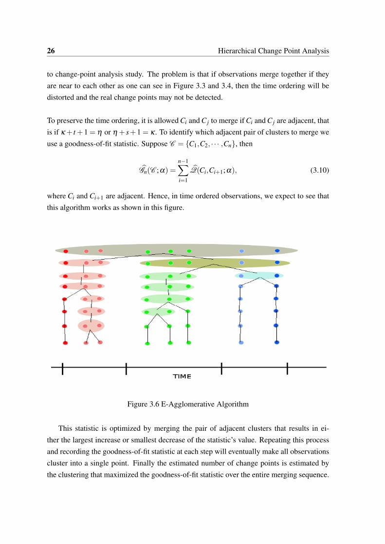
To preserve the time ordering, it is allowed Ci and C j to merge if Ci and C j are adjacent, thatis if κ + t +1 = η or η + s+1 = κ . To identify which adjacent pair of clusters to merge weuse a goodness-of-fit statistic. Suppose C = C1,C2, · · · ,Cn, then
Gn(C ;α) =n−1∑i=1
Q(Ci,Ci+1;α), (3.10)
where Ci and Ci+1 are adjacent. Hence, in time ordered observations, we expect to see thatthis algorithm works as shown in this figure.
Figure 3.6 E-Agglomerative Algorithm
This statistic is optimized by merging the pair of adjacent clusters that results in ei-ther the largest increase or smallest decrease of the statistic’s value. Repeating this processand recording the goodness-of-fit statistic at each step will eventually make all observationscluster into a single point. Finally the estimated number of change points is estimated bythe clustering that maximized the goodness-of-fit statistic over the entire merging sequence.

3.3 Change Point Estimation 27
The algorithm of this method can be seen in the appendix.
Overfitting is always a concern in change point analysis. As in Bai and Perron (1998)[2], we also need a penalty function to alleviate the overfitting problem. Thus, the changepoint locations are estimated by maximizing
GK = GK +Penalty, (3.11)
where K is the number of change points. Naturally, a penalty function can be Penalty=−K.
3.3.3 Significance Testing
As mentioned earlier, since the distributions of observations are not known, a non-parametric testing method is required. Here, we also use the resampling method proposedby Matteson and James (2013) [19]. To be specific, the method they employ is a permuta-tion test. The method will help us determine the statistical significance of a change pointgiven previously estimated change points. This test can also serve as a stopping criterionfor the proposed iterative estimation procedure. Suppose that we have already found κ −1change points which give us κ clusters. For a newly detected change point τκ , the asso-ciated test statistic is qκ . If the value of qκ , as in (3.9), is above the critical value, then asignificant change in distribution within one of the existing clusters is detected. However, aprecise critical value is not feasible without any knowledge of the underlying distributions.Therefore, a permutation test is needed to solve this puzzle.
Under the null hypothesis of no additional change points, a permutation test works as fol-lows. Note that the permutation test only performs within but not across clusters. First ofall, the observations within each cluster are permuted to construct a new sequence of lengthT . This yields T ! new samples with equal probabilities. Afterwards, the same estimationprocedure is applied to the newly permuted sequence. Note that if we have a very long se-quence, for example more than 700 observations in our swing fund study, this method willbecome piratically unfeasible because the number of all possible permutations can be reallylarge. Hence, in this thesis we follow the number of random permutations suggested by theauthors, which is 499. It means that the resampling will just gives 499 random permutationsregardless the sample’s length. With this number, the permutation will be repeated and afterrthe permutation of the observations we record the value of the test statistic q(r)κ . Then, an

28 Hierarchical Change Point Analysis
approximate p-value is defined as
p =
∑R+1r=1 1r:q(r)κ ≥qκ(R+1)
. (3.12)
If we fix the significance level at p0 = 0.05, then the rejection criterion is p ≥ p0 and thedetection algorithm terminates. Otherwise, the procedure estimates an additional location.This permutation test may be performed after the E-Divisive procedure reaches a predeter-mined number of clusters to quickly provide initial estimates. Also note that this procedureis subject to the autocorrelation of the observations. We will take into account this issue inChapter 5.
3.4 Time Series Analysis
The underlying assumption of the e-distance measure is that the observations have tobe independent, which is however usually not true for time ordered observations. In timeseries analysis, one may encounter autocorrelation problems. In our swing pricing study,the market excess return defined in Chapter 2 is free of autocorrelation by definition. Theflow percentage is defined as the ratio of fund flow at day t to the fund size at day t − 1.By the pricing rule of a mutual fund, the fund price is usually correlated with that one daybefore. Hence, the vector of flow percentage is exposed to the problem of autocorrelationtoo, and that will jeopardize the underlying assumption of the distance measurement. Inreality, if a fund is not actively traded, for example if there are some days where the fundsare not traded at all, then the severity of autocorrelation in the vector of flow percentage willbe downgraded. From our experience we note that a change in swing pricing policy oftenindicates a shift in correlation between the vector of market excess return and the vector offlow percentage. To capture this concurrent relationship, we need another model.
A model taking into account/approximating multivariate dynamic relationships is the VAR(p),vector autoregression of order p. Suppose a VAR(p) model of the 2×1 vector of time seriesyt = (y1t ,y2t) with autoregressive order p:
yt = c+A1yt−1 + · · ·+Apyt−p +νt ,

3.4 Time Series Analysis 29
where Ai are 2×2 coefficients martices and c is a 2×1 of vector of intercepts. νt is a 2×1vector of disturbances that have the following properties:
E(νt) = 0,
E(νtν ′t ) = Σν ,
E(νtν ′s) = 0.
By the assumptions, we know that νt is a sequence of serially uncorrelated random vectorswith concurrent full rank covariance matrix Σ. The concurrent relationship between y1 andy2 is measured by the off-diagonal elements of Σ. Replace y1 and y2 by e and F definedin Chapter 2 to make the VAR(p) model relevant to our study. In our swing pricing study,we use a VAR(2) model for the funds employed. Even there are some funds that do nothave the problem of serial correlation, we will still apply the VAR model to them in order tosolve the more general problem. Hence, the hierarchical change point technique based onthe e-distance measurement will be applied to the disturbance vector.

Chapter 4
Simulation
In the first section of this chapter we show two simulation examples provided by Mat-teson and James (2013) [18]. In this section we see the performance of the nonparametricmethods applied on independent sequences . Since our study is based on time series anal-ysis, we also aim to examine if the change-point detection methods based on hierarchialclustering can still work when the observations are serially correlated. Thus we also simu-late an autocorrelated multivariate sequence to see the performance of these methods.
4.1 Independent Sequences
We begin with the simple case of identifying change in univariate normal distributions.For this we sequentially generate 100 independent samples from the following normal dis-tributions:
N ∼ (0,1), N ∼ (0,√
3), N ∼ (2,1), and N ∼ (2,2)
If we let α = 1, the E-Divisive method identifies 108, 201 and 308 with p-values of 0.002,0.002 and 0.010 respectively. The E-Agglomerative method gives similar results, 101, 201and 301 with p-values of 0.004, 0.002 and 0.012 respectively. In the following figurewe can see a simulated independent Gaussian observations with changes in mean or vari-ance. Dashed vertical lines indicate the change point locations estimated by the E-Divisivemethod, when using α = 1. Solid vertical lines indicate the true change point locations.

4.1 Independent Sequences 31
Time
Val
ue
0 100 200 300 400
−5
05
10
Figure 4.1 Change in a Univariate Gaussian Sequence
As mentioned in Chapter 2, we suspect that the threshold change in a swing pricing pol-icy can be seen as a change in the correlation between the vector of the market excess returnand the vector of flow percentage. Hence, we will consider the case where the marginaldistributions remain the same, but the joint distribution changes. Suppose that we have abivariate normal distributions with the mean vector µ = (0,0,0)⊤ and the following covari-ance matrices:
1 0 00 1 00 0 1
,
1 0.9 0.90.9 1 0.90.9 0.9 1
, and
1 0 00 1 00 0 1
.
We use the R package procedure mvtnorm to generate the observations. We will generate250 normal observations with each of covariance matrices mentioned above. Hence in totalwe have 750 observations. Thus among the 750 observations there are 2 change points, 251and 501 respectively. We will use both the E-Divisive and the E-Agglomerative method todetect the change points. By the E-Divisive method, we have detected the change pointson 251 and 502 with p-values of 0.002 and 0.002 respectively. By the E-Agglomerativemethod, we have detected the change points at 301 and 501 with p-values of 0.002 and0.005 respectively. The results are the same as those shown in [18]. We also find that forthe first change point detected by the E-Agglomerative method is lagged by 50 observations.

32 Simulation
In the previous example, we locate the change points at equal distances in our simulatedrandom vectors. To test how the hierarchial change point technique works in a more generalscenario, we will place the change points unequally through the simulated random vectors.For example, we will generate 150 multi-normal random observations with covariance ofzero, 300 multi-normal random observations with covariance of 0.9, 300 random observa-tions with covariances of 0. The change points detected by the E-Divisive method are 151and 454 with p-values of 0.002 and 0.002 respectively. For the E-Agglomerative method,we find 158 and 452 where the underlying distribution changes, with p-values of 0.004 and0.004 respectively. We see that the E-Divisive and the E-Agglomerative methods generatesatisfying results for independent sequences.
4.2 Autocorrelated Sequence
In the section, we aim to test the performance of the hierarchial nonparametric changepoint method on a stationary but autocorrelated process. A stochastic process yt is station-ary if its first and second moments are time invariant: in particular if E[yt ] = µ , ∀t andE[(yt − µ)(yt−h − µ)⊤] = ΓY (h) = ΓY (−h)⊤,∀t,h = 0,1,2, · · · , where µ is a vector of fi-nite mean terms, and ΓY (h) is a matrix of finite covariances. The best model (in termsof tractability) we can think of is a multivariate Gaussian process, where we can form thecovariance matrix easily. Hence, we will assume that the underlying distribution of the au-tocorrelated process is normal. Although in Chapter 3 we suggest to use the residual vectorof a VAR(p) process to avoid dependency problem, the empirical finding in our study is thatthe correlation between the market excess return and the flow percentage change in a fundwill increase if there is swing pricing policy implemented. The observations of flow per-centage may be autocorrelated as discussed in Chapter 3. However, we want to investigatea more general problem, thus we will look at two autocorrelated process, X and Y , of whichthe correlation changes over time.
We start from autocorrelation at lag 1. The problem can be stated as follows. We wantto simulate two process Xt = a1Xt−1 + θt and Yt = a2Yt−1 +ωt such that corr(Xt ,Yt) = ρ .We can also write these two process as[
Xt
Yt
]=
[a1 00 a2
]×
[Xt−1
Yt−1
]+
[θt
ωt
](4.1)

4.2 Autocorrelated Sequence 33
This is a VAR(1) process: Zt = FZt−1 +ηt , where Zt and ηt are
[Xt
Yt
]and
[θt
ωt
]respec-
tively. F is the coefficient matrix. ηt is a 2-dimensional zero mean white noise process. It isassumed that E[Zt−1η⊤
t ] = 0. We post-multiply by its own transpose and take expectations,then we have
E[ZtZ⊤t ] = FE[Zt−1Z⊤
t−1]F⊤+E[ηtη⊤
t ].
Let’s denote the covariance matrix of Zt by Σ and that of ηt by Q, then we have
Σ = FΣF⊤+Q,
where the residuals are assumed to have unit variances. Denote the component of Σ as σand that of Q by q. For the sake of convenience, we use 1 to stand for X and θ and 2 for Y
and ω , then
Σ =
[σ11 σ12
σ21 σ22
],Q =
[1 q12
q21 1
].
This equation needs to be solved by applying the two properties of vectorization: vec(A+
C) = vec(A)+vec(C) and vec(ABC) = (C⊤⊗A)vec(B). Then the solution will be
vec(Σ) = [I −F⊤⊗F ]−1 vec(Q),
where vec stands for the vectorization and ⊗ for the Kronecker product and I is the identitymatrix.
Since we are dealing with 2× 2 matrices and for convenience we assume that the errorterms have unit variances, it is not hard to write this out precisely:
σ11
σ12
σ21
σ22
=
1−a21 0 0 0
0 1−a1a2 0 00 0 1−a1a2 00 0 0 1−a2
2
−1
×
1
q12
q21
1
.

34 Simulation
Now the desired correlation is
ρ =σ21√
σ11σ22=
q12
√(1−a2
1)(1−a22)
1−a1a2.
Hence, to generate two AR(1) process with desired correlation we need to generate theresiduals θt and ωt with unit variances and correlation
corr(θt ,ωt) = ρ1−a1a2√
(1−a21)(1−a2
2).
We can verify that this method indeed works via the following code in R:
> set.seed(1988)
> calculaterho<-function(rho,rho1,rho2)
+rho*(1-rho1*rho2)/sqrt((1-rho1^2)*(1-rho2^2))
> burn.in<-300
> n<-300
> rho<-0.8
> a1<-0.5
> a2<-0.5
> q12<-calcrho(rho,rho1,rho2)
> eps<-mvrnorm(n+burn.in,
+mu=c(0,0),Sigma=cbind(c(1,q12),c(q12,1)))
> x<-arima.sim(list(ar=a1),n,innov=eps[burn.in+1:n,1]
+,start.innov=eps[1:burn.in,1])
> y<-arima.sim(list(ar=a2),n,innov=eps[burn.in+1:n,2]
+,start.innov=eps[1:burn.in,2]).
> cor(x,y)
[1] 0.7715924
We can see the correlation between X and Y is very close to 0.8.
After verifying that our method can generate the desired correlation between two autore-gressive processes, we try if the hierarchical change point detection method will help usfind the break points without the assumption of independence. We first look at a general

4.2 Autocorrelated Sequence 35
case where the parameters of the autoregressive processes change and so does the correla-tion between them. Let’s assume that there are 4 segments of 1000 simulated values for eachprocess. The 1000 simulated values will be equally divided, hence there are 250 for eachsegment. For the first segment, let the parameters a1 and a2 be 0.5 and 0.5. The correlationbetween the two processes is 0. For the second segment, the correlation coefficient becomes0.8 and a1 and a2 remain the same. The ρ will increase to one, a1 is 0.1 and a2 is 0.9 in thethird segment. In the last segment all parameters are the same as that in the first segment.These two processes are illustrated in the following figure.
0 200 400 600 800 1000−5
0
5X
0 200 400 600 800 1000−5
0
5
10Y
Figure 4.2 Changes in Correlation and Paremeters
Applying the E-Divisive and the E-Agglomertative method, we find these change points:
Table 4.1 Deteced Change Points in Simulatied VAR(1)
E-Divisive 82 194 444 520 661p-value (0.004) (0.036) (0.018) (0.018) (0.002)E-Agglo 158 402 592 696p-value (0.013) (0.04) (0.021) (0.003)

36 Simulation
We can see from the table above that the change points detected by the E-Divisive andthe E-Agglomerative method are not satisfying. We also question whether the simulatedprocesses are too complicated. They largely weaken the method by the violation of inde-pendence assumption due to the complexity. Hence, we will generate two simple processesand see if the performance of two nonparametric methods can be improved. We generatetwo other processes for each 900 observations. a1 and a2 remain at 0.5 and 0.5 for the entiresimulation. The simulation is divided into 3 segments equally. The change is only in thecorrelation For the first and last segments the correlation coefficients between two processesare 0. We put the change point at 300 with the correlation coefficient of 0.8.
0 100 200 300 400 500 600 700 800 900−5
0
5X
0 100 200 300 400 500 600 700 800 900−5
0
5Y
Figure 4.3 Only Correlation Change
Employing the two change point detection methods again, we find the following:

4.2 Autocorrelated Sequence 37
Table 4.2 Detected Correlation Change in Simulatied VAR(1)
E-Divisive 302 407 844p-value (0.02 ) (0.04) (0.016)E-Agglo 307 466p-value (0.002 ) (0.04)
Now we see that the first change point is detected via both methods. Unfortunately, theyalso generate other change points that we know are not. If we lower the significance levelto 1%, then the second change point generated by the E-Agglomerative is not significantanymore. Hence, the E-Agglomerative will give the correct change point based on our sim-ulation. However, we may encounter more complicated changes in time series observations.After our simulation trial, we do not expect that these two nonparametric methods are freeof the independence assumption. As a result, we will deal with the autocorrelation problemas discussed in Chapter 3.

Chapter 5
Empirical Results
5.1 Data Description
We apply the methodology on a sample of high yield funds with UCITS status. Thesample funds are domiciled in Luxembourg or Ireland, the largest and second largest domi-ciles for funds that are offered cross-border. We selected funds from three high yield bondcategories, specifically EUR High Yield Bond, Europe High Yield Bond and USD HighYield Bond, as for these categories of funds we expect a favorable signal-to-noise ratio. Bythis we mean high transaction costs in the underlying securities, resulting in a high swingfactor, in combination with relatively low daily tracking errors on days when there is noswing pricing . We analyze funds in the three-year period 2011-2013.
The data needed for the analysis consists of daily NAVs and daily number of outstand-ing shares for all fund share classes as well as the dividend history. Based on this data,we calculate daily fund total returns and daily net flows. Furthermore, the analysis requiresdaily benchmark data, which, together with fund returns, is used to calculate daily marketexcess returns. We obtain this data from Morningstar Direct throughout the 3-year researchperiod. We will use 3 funds to illustrate our methodologies. They are JPM Europe HighYield Bond, CS BF (Lux) High Yield and Natixis Euro High Income Fd respectively. Wehave put the information of these funds in the following table. Share Classes refer to thenumber of share classes existed in a fund.

5.1 Data Description 39
Table 5.1 Fund Info
Fund FundID Morningstar Category Share Classes
JPM Europe FSGBR057TP Europe OE Europe 8High Yield Bond High Yield Bond
CS BF (Lux) FSGBR057TP Europe OE USD 4High Yield High Yield Bond
Natixis Euro FSGBR057TP Europe OE EUR 8High Income Fd High Yield Bond
We also managed the data to match the reality. In general, Number of Shares is pub-lished one day later than NAVs, although some funds do publish these parameters on thesame day. Our approach is looking up for the data of Number of Shares of a share classin a fund at the inception date. If the NAV of that share class is published on the sameday, then we will not shift the data of Number of Shares one day upward to match it NAVs.Otherwise we will do so. We also removed all weekends and holidays for both funds’ andholidays’. Note that one has to shift the data of Number of Shares (if it is necessary) beforeremoveing the weekends and holidays. After managing the data, we are able to calculate themarket excess return and flow percentage descried in Chapter 2. The purpose of the analysisundertaken in this thesis is to explore the impact of a change-point detection technique onthe finding the threshold of a fund’s swing pricing policy. A summary of the sample anddescriptive statistics for the market excess return of each fund is in the table below.
Table 5.2 Sample Market Excess Returns
Fund Mean Median Min Max Std Obs
JPM Europe -0.000309 -0.000524 -0.041703 0.013835 0.004815 749High Yield Bond
CS BF (Lux) -0.000143 0.008592 -0.000173 -0.004667 0.001258 748High Yield
Natixis Euro -9.25E-05 0.021332 -8.13E-05 -0.02136 0.002663 752High Income Fd
The following table is the sample and descriptive statistics for flow percentage.

40 Empirical Results
Table 5.3 Sample Flow Percentage
Fund Mean Median Min Max Std Obs
JPM Europe 0.000712 4.69E-05 -0.163188 0.054204 0.014829 749High Yield Bond
CS BF (Lux) 0.006285 5.060103 2.81E-05 -0.525137 0.186314 748High Yield
Natixis Euro 0.00124 0.336815 0 -0.047159 0.014392 752High Income Fd
We also investigate the serial dependence within observations, because the change-pointdetection methods described in Chapter 3 assume that the sample is not dependent overtime. Although we observed a few significant serial correlation within the observations forboth market excess returns and flow percentage, we just neglected them as in many othertextbooks. Also note that the tests are performed at the significance level of 5%, we wouldexpect that all the significant autocorrelation will disappear at a 10% significance level. Thecorrelogram in the disturbance vector of the vector autoregressive in Section 3.4 with twolags can be seen in the following 3 figures.
Figure 5.1 Correlogram of JPM

5.1 Data Description 41
Figure 5.2 Correlogram of CS
Figure 5.3 Correlogram of Natixis
In these figure, the vertical axis is the significance level. The upper and lower dashlines in these figures are indicated as significance level boundaries. In other words, if thecorrelation value does not exceed either the upper or the lower dash line, we will concludethat there is no significant correlation exists in two variables. As one can see in these figures,the input variables do not have very significant autocorrelation. The following table givesthe thresholds detected by our threshold finder model without applying any change-pointdetection study.

42 Empirical Results
Table 5.4 Thresholds Detected without Change Point Study
Fund Threshold
JPM 1.00%(81%)
CS BF 0.88%(23%)
Natixis 1.80%(34%)
The percentage numbers in brackets stand for the ratio of abnormal market excess returnsexplained by swing pricing policy. We see that if we only apply the threshold finder modelto these funds, only JPM fund seems to have swing policy. The threshold and the ratio ofthis fund indicate that the swing pricing policy for this fund is stable and remains unchangedduring our sample period. The model can also detect the swing threshold for the other twofunds. However, the ratio is not satisfying. In the following section, one can see that if wedetect the change point in the two time ordering vectors, e and F , we will have a differentscenario.
5.2 Empirical Threshold and Change Points
First of all, we perform the method proposed by Bai and Perron in Chapter 2 to detectthe break points in our funds. Afterwards, we use our threshold finder model to find thethreshold for each subperiod. We will use this method as a benchmark to compare withthe E-Divisive and the E-Agglomerative method described in Chapter 3. The comparisoncriterion the ratio of abnormal market excess returns explained by swing pricing. The resultsgenerated by this method are given in the following tables.

5.2 Empirical Threshold and Change Points 43
Table 5.5 Detected Change Points (Bai and Perron)
Fund Change 1 Change 2 Change 3 Change 4
JPM 655p-value 0.98CS BF 358 520 636p-value 0.016 0.62 0.00Natixis 172 286 484 602p-value 0.00 0.83 0.00 0.03
From the above table, we note that there are some change points that are not significantbecause they have very large p-values. If a change point is not significant, we do not take itinto account as a regime change in swing policy.
Table 5.6 Swing Pricing Threshold (Bai and Perron)
Fund Threshold 1 Period Threshold 2 Period
JPM 1.00% 01/01/2009-(81%) 31/12/2013
CS BF 2.00% 18/03/2013-(90%) 31/12/2013
Natixis 2.50% 04/12/2012- 4.00% 03/06/2013-(87.5%) 31/05/2013 (100%) 31/12/2013
For JPM, we see that because the change point is not significant, we run the thresholdfinder model for the whole sample period and detect the threshold of 1%. It catches ourattention that for CS BF and Natixis, the first change point of each fund is significant. How-ever, we do not detect the threshold for these funds during the period prior to the changepoint. That is why in the table above we do not mention the period before the first detectedchange point for each fund. We note that Natixis Euro High Income Fd did not implementswing pricing policy in the end of 2012, and it changed after half a year. This is an interest-ing fund because it captures a real swing pricing policy change. We draw the movements ofthis fund’s market excess return and flow percentage into picture to illustrate the mechanismof swing pricing.
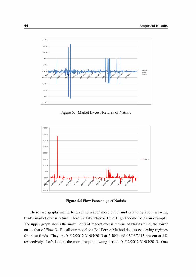
44 Empirical Results
Figure 5.4 Market Excess Returns of Natixis
Figure 5.5 Flow Percentage of Natixis
These two graphs intend to give the reader more direct understanding about a swingfund’s market excess return. Here we take Natixis Euro High Income Fd as an example.The upper graph shows the movements of market excess returns of Naxitis fund, the lowerone is that of Flow %. Recall our model via Bai-Perron Method detects two swing regimesfor these funds. They are 04/12/2012-31/05/2013 at 2.50% and 03/06/2013-present at 4%respectively. Let’s look at the more frequent swung period, 04/12/2012-31/05/2013. One

5.2 Empirical Threshold and Change Points 45
can see that a lot spikes gather in this period, above 2.5%. Most of these spikes point up-ward. The correspondent market excess returns are also very volatile, and move upward anddownward in the almost the same magnitude.
Applying the methodology discussed in Chapter 3, we find the following change pointsfor these 3 funds.
Table 5.7 Detected Change Points (E-Divisive)
Fund Change 1 Change 2 Change 3
JPM 629p-value 0.112CS BF 359 588p-value 0.02 0.07Natixis 498 531 599p-value 0.00 0.83 0.05
Table 5.8 Detected Change Points (E-Agglomerative)
Fund Change 1 Change 2 Change 3
JPM 688p-value 0.39CS BF 358 629p-value 0.02 0.05Natixis 509 596 617p-value 0.00 0.27 0.002
The above two tables give the change points detected by the two nonparametric methodsdiscussed in Chapter 3. For JPM, both method do not find any significant change point. ForCS BF, there are two change points detected. The first change point is almost the same bythese two methods. However, the second one is slightly different. For Natixis, the 3 changepoints are different. The result is also in line with that in Matteson and James (2013) [19].The change points generated by the two methods are different, and the E-Agglomerativeusually gives the change dates that are later than the E-Divisive does. After knowing thechange points, we shall see what effects these methods make on swing pricing thresholddetection.

46 Empirical Results
For JPM, the swing pricing policy does not change in our sample period, hence the thresholdfinder model applies to the whole sample period and the swing pricing threshold embeddedin this fund remain unchanged, 1%. The swing regime changes based on these two methodsare in the following table.
Table 5.9 Thresholds by Hierarchical Methods
Fund Threshold 1 Period Threshold 2 Period
CS BF 2.00% 22/12/2013-(E-Divisive) (75%) 31/12/2013
CS BF 2.00% 10/03/2013-(E-Agglo) (90%) 31/12/2013
Natixis 2.50% 21/12/2012- 4% 03/06/2013(E-Divisive) (100%) 31/05/2013 (100%) 31/12/2013
Natixis 3.50% 10/01/2013-(E-Agglo) (87.5%) 31/12/2013
In general, one can see that the three change-point detection methods combined withour threshold finder model comprise with the regime changes to some extent. For the JPMfund, we find that the swing regime is implemented before the starting date in our sample.For the CS fund, we see that swing pricing policy is implemented in the late part of thesample period. After the swing pricing policy is implemented, it seems stable for the rest ofthe period. For the Natixis fund, we find that there are multiple swing regimes and differentswing pricing thresholds. We also see that for CS fund, Bai-Perron, E-Divisive and E-Agglomerative methods give the same threshold. The E-Divisive lowers the ratio for thisfund by 15%. However, the E-Agglomerative method shows that the swing pricing thresholdis the same as the one detected with Bai-Perron method, although the swing period is a bitdifferent. However, for Natixis, the thresholds detected by the E-Agglomerative method isdifferent. If we just look at the ratios, it seems that E-Divisive method performs better thanother two methods. By this method, one will conclude that Natixis fund is swung and hastwo different swing regime.

Chapter 6
Conclusion
The swing pricing policy intends to protect the investors from the volatile prices causedby the trading volume. In this thesis, we develop a unique method of finding the thresholdof the trading volume that triggers the swing pricing in a mutual fund. The method is basedon the simulated value of the market excess returns for potential swing pacing thresholds.The magnitude of trading is classified as big or small, so is that of market excess of returns.It is expected that a large market excess return is paralleled by a large trading volume. Thethreshold detection model can work for the funds of which the swing pricing policies do notchange. However, A fund’s swing pricing policy may change. For example, the board mem-bers may decide to increase the swing pricing threshold for investors dislike volatile prices.Without knowing the changes of the swing policy, the threshold detection model will notwork. That requires a change-point detection method that can be employed to multivariatedistributions and that is able to adapt to multiple changes.
We initially use the Bai-Perron method. It suggests that the optimal number of changepoints will minimize the sum of squared residuals. This method gives us satisfactory re-sults. We also want to investigate whether there are alternative methods that can improvethe threshold detection results. Therefore we use a newly developed method which is basedon hierarchial clustering. The new nonparametric method includes two different methods ofclustering, divisive and agglomerative. The new method does not have any assumptions onthe underlying distributions of observations, but does assume that the observation sequenceneeds to be independent. After applying the new method, the empirical results indicate thatfor Natixis fund the E-Agglomerative method indeed performs the better than the other one.For other funds these methods perform similarly. Hence we cannot conclude that the newmethod is an improver.

48 Conclusion
For the models, there are still some improvements required. For the threshold detectionmodel, how to measure the magnitude of market excess return is difficult. We have giventhe definition of "hurdle rate" for this measurement. Once the value of market excess returnis above the hurdle rate, we say that there is a jump in the market excess return which maybe caused by the swing pricing policy. The difficulty is not only in the jump detection, butalso in matching the swing pattern. At the end of a swing pattern, one expects that thereis also a jump in the contrary direction of that of flow percentage in the previous day. Forthe hierarchical change point analysis, it is assumed that the observations are independent.However, for time ordered data it is difficult to meet this assumption. We show that forautocorrelated observations, this method does not give us satisfying results.

Bibliography
[1] D.W.K. Andrews. Test for parameter instability and structural change with unkownchange point. Econometrica, 61, 1987.
[2] J. Bai and P. Perron. Estimating and testing linear models with multiple structuralchanges. Econometrica, 66(4), 1998.
[3] J. Bai and P. Perron. Computation and analysis of multiple structural change models.Journal of Applied Econometrics, 18(1), 2003.
[4] R. Ball and P. Brown. An empirical evaluation of accounting income numbers. Journalof Accounting Research, 6(2), 1968.
[5] M. Basseville and I.V. Nikiforov. Detection of Abrupt Changes - Theory and Applica-tion. Prentice-Hall, Inc., Englewood Cliffs, N.J.), 1993.
[6] R. Davis, T. Lee, and C. Rodriguez-Yam. Structural break estimation for nonstationarytime series models. Journal of the American Statistical Association, 101(473), 2008.
[7] C. Erdman and J.W. Emerson. bcp: An r package for performing a bayesian analysisof change point problems. Journal of Statistical Software, 23(3), 2007.
[8] E. Fama, L. Fisher, M.C. Jansen, and R. Roll. The adjustment of stock prices to newinformation. International Economic Review, 10(1), 1969.
[9] S. B. Hariz, J. J. Wylie, , and Q. Zhang. Optimal rate of convergence for nonparametricchange-point estimators for nonstationary sequences. The Annals of Statistics, 35(4),2007.
[10] Y. Kawahara and M. Sugiyama. Sequential change-point detection based on directdensity-ratio estimation. Statistical Analysis and Data Mining, 5(2), 2011.
[11] R. Killick and I. Eckley. changepoint: An r package for changepoint analysis. Journalof Statistical Software, 58(3), 2011.
[12] R. Killick, P. Fearnhead, and I. Eckley. Optimal detection of changepoints with a linearcomputational cost. Journal of the American Statistical Association, 107(500), 2012.
[13] G.N. Lance and W.T. Williams. A general theory of classificatory sorting strategies.Computer Journal, 9(4), 1967.

50 Bibliography
[14] N. Lange, B.P. Carlin, and A.E. Gelfand. Hierarchal bayes models for the progres-sion of hiv infection using longitudinal cd4 t-cell numbers. Journal of the AmericanStatistical Association, 87(419), 1992.
[15] M. Lavielle and G. Teyssiere. Detection of multiple change-points in multiple time-series. Lithuanian Mathematical Journal, 46(4), 2006.
[16] Lipper. Symbiosis in the evolution of ucits; 1988 - 2018 : Three decades of fundsindustry transformation. 2010.
[17] A. Lung-Yut-Fong, C. Levy-Leduc, and O. Cappe. Homogeneity and change-pointdetection tests for multivariate data using rank statistics. arXiv:1107.1971, 2011.
[18] D.S. Matteson and N.A. James. ecp: An r package for nonparametric multiple changepoint analysis of multivariate data. arXiv:1309.3295v2, 2013.
[19] D.S. Matteson and N.A. James. A nonparametric approach for multiple change pointanalysis of multivariate data. Journal of the American Statistical Association, To ap-pear, 2013.
[20] G. W. Milligan. An examination of the effect of six types of error perturbation onfifteen clustering algorithms. Psychometrika, 45(3), 2003.
[21] W.K. Newey and K.D. West. A simple, positive semi-definite, heteroskedasticity andautocorrelation consistent covariance matrix. Econometrica, 55(3), 1987.
[22] E.S. Page. Continuous inspection schemes. Biometrika, 41(1/2), 1954.
[23] M.L. Rizzo and G.J. Szekely. Disco analysis: A nonparametric extension of analysisof variance. Annals of Applied Statistics, 4(2), 2010.
[24] G.J. Ross and N.M. Adams. Two nonparametric control charts for detecting arbitrarydistribution changes. Journal of Quatlity Technology, 44(2), 2012.
[25] B.M.J. Slot. Iedereen kapitalist; de ontwikkeling van het beleggingsfonds in nederlandgedurende de 20ste eeuw. (dissertation, Aksant, Amsterdam), 2004.
[26] G.J. Szekely and M.L Rizzo. Hierarchical clustering via joint between-within dis-tances: Extending ward’s minimum variance method. Journal of Classication, 22(2), 2005.
[27] E. Venkatraman. Consistency results in multiple change-point problems. PhD thesis,Stanford University, 1992.
[28] Jr. Ward, J. H. Hierarchical grouping to optimize an objective function. Journal of theAmerican Statistical Association, 58(301), 1963.
[29] R.T. Wilcox. Bargain hunting or star gazing? how consumers choose mutual funds.Journal of Business, 76(4), 2003.
[30] Y.C. Yao. Estimating the number of change-points via schwarz criterion. Statisticsand Probability Letters, 6, 1987.

Appendix A
Change-Point Detection Algorithm
A.1 E-Divisive Algorithm
Data: Observations X, significance level p0, minimum segment m, R=499, αResult: A segmentation of the observationsCreate Distance Matrix Xα
i j =∣∣Xi −X j
∣∣α ;
while Have not found an insignificant change point doEstimate next change point location;Test the significance of the estimated change point;if This is a significant change point then
Update the segmentation;end
endreturn Final Segmentation
Algorithm 2: Outline of E-Divisive Algorithm

52 Change-Point Detection Algorithm
A.2 E-Agglomerative Algorithm
Data: Initial Segmentation C, observation X, penalty function, andResult: A segmentation of the observationsCreate Distance Matrix Di, j = E (Ci,C j;α);Obtain initial penalized goodness-of-fit statistic;for K ∈ N,N +1, · · · ,2N −3 do
Merge best segments;Update current goodness-of-fit statistic;if Current statistic ≤ largest statistic so far then
Update largest statistic;end
endPenalize the sequence of obtained goodness-of-fit statisticChoose optimal segmentation based on penalized goodness-of-fit statistic;return Optimal Segmentation
Algorithm 3: Outline of E-Divisive Algorithm

Appendix B
Some Matlab Codes
B.1 Threshold Finder Model
1 function [threshold,hits,error]=Thresholdfinder2(L,Emb,flow,Ex,Tr)
2 % Emb is the vector contains the higher
3 % and lower bound of the range of normal market
4 % exceess return,Ex is the market excess vector,
5 % Tr is the vector of flow percentage
6 % L is the vector length,
7 % flow is the under bound of the flow percentage
8 % we set the value of 'flow' to be 20%.
9 threshold=zeros(3,1);
10 for l=1:1
11 for i=1:L
12 if Ex(i)>=Emb(1,:)
13 sp(i,:)=1;
14 elseif Ex(i)<=-Emb(2,:)
15 sp(i,:)=-1;
16 else sp(i,:)=0;
17 end
18 end
19 thr=0:0.0001:flow;
20 n=flow/0.0001;
21 for i=1:n
22 for j=1:L
23 if Tr(j)>= thr(i)
24 TC(j,i)=1;

54 Some Matlab Codes
25 elseif Tr(j)<=-1*thr(i)
26 TC(j,i)=-1;
27 else TC(j,i)=0;
28 end
29 end
30 end
31 M=zeros(L,n);
32 for i=1:n
33 for j=1:L-1
34 if abs(TC(j,i))==1
35 M(j,i)=TC(j,i);
36 for k=j:L-1
37 if TC(k,i)*TC(k+1,i)==-1;
38 M(k+1,i)=TC(k+1,i);
39 elseif TC(k,i)*TC(k+1,i)==1;
40 M(k+1,i)=0;
41 elseif TC(k,i)*TC(k+1,i)==0&&abs(TC(k,i))==1
42 M(k+1,i)=-TC(k,i);
43 elseif TC(k,i)*TC(k+1,i)==0&&abs(TC(k+1,i))==1
44 M(k+1,i)=TC(k+1,i);
45 else
46 M(k+1,i)=0;
47 end
48 end
49 end
50 end
51 end
52 N=zeros(L,n);
53 for i=1:n
54 for j=1:L-1
55 if M(j,i)*M(j+1,i)==1&&abs(M(j,i))==1
56 N(j+1,i)=-M(j+1,i);
57 end
58 end
59 end
60 NN=M+N;
61 for i=1:n
62 for j=1:L
63 if NN(j,i)==sp(j,1)&&abs(sp(j,1))==1&&abs(TC(j,i))==1
64 I(j,i)=1;
65 else I(j,i)=0;
66 end

B.1 Threshold Finder Model 55
67 end
68 end
69
70 err=sum(I,1);
71 hits=max(err);
72 [v,c]=max(err);
73 flowthreshold=(thr(:,c));
74 for i=1:n
75 for j=1:L
76 if NN(j,i)==sp(j,1)
77 I(j,i)=1;
78 else I(j,i)=0;
79 end
80 end
81 end
82 ERR=zeros(L,n);
83 for i=1:n
84 for j=1:L
85 if I(j,i)==0&&abs(TC(j,i))==1&&sp(j,1)==0
86 ERR(j,i)=1;
87 end
88 end
89 end
90 Err=sum(ERR,1);
91 error=Err(:,c);
92 threshold(1,l)=flowthreshold;
93 threshold(2,l)=hits;
94 threshold(3,l)=error;
95 end
96 end

56 Some Matlab Codes
B.2 The E-Divisive Distance
1 %This code is developed by Szekely and Rizzo
2 function L = elinkage(y, alpha)
3 ed = 2 .* (squareform(pdist(y)).^alpha);
4 n = length(ed);
5 csize = ones(1, n);
6 cindex = 1:n;
7 L = zeros(n-1, 3);
8 nclus = n;
9 for merging = 1:(n-2);
10 b = ones(nclus, 1) .* (ed(1,2) + 1);
11 B = ed + diag(b);
12 [colmins, mini] = min(B);
13 [minmin, j] = min(colmins);
14 i = mini(j);
15 L(merging, 1) = cindex(i);
16 L(merging, 2) = cindex(j);
17 L(merging, 3) = ed(i, j);
18 m1 = csize(i);
19 m2 = csize(j);
20 m12 = m1 + m2;
21 for k = 1:nclus;
22 if (k ~= i && k ~= j);
23 m3 = csize(k);
24 m = m12 + m3;
25 ed(i, k) = ((m1+m3)*ed(i,k) + (m2+m3)*ed(j,k) - m3*ed(i,j))/m;
26 ed(k, i) = ed(i, k);
27 end;
28 end;
29 ed(j, :) = [];
30 ed(:, j) = [];
31 csize(i) = m12;
32 csize(j) = [];
33 cindex(i) = n + merging;
34 cindex(j) = [];
35 nclus = n - merging;
36 if L(merging, 1) > L(merging, 2);
37 ij = L(merging, 1);
38 L(merging, 1) = L(merging, 2);
39 L(merging, 2) = ij;

B.2 The E-Divisive Distance 57
40 end;
41 end;
42 L(n-1, :) = [cindex(1), cindex(2), ed(1, 2)];
43 if L(n-1, 1) > L(n-1, 2);
44 ij = L(n-1, 1);
45 L(n-1, 1) = L(n-1, 2);
46 L(n-1, 2) = ij;
47 end
