changes in continental freshwater discharge from … in continental freshwater discharge from 1948...

Changes in Continental Freshwater Discharge from 1948 to 2004

AIGUO DAI, TAOTAO QIAN, AND KEVIN E. TRENBERTH

National Center for Atmospheric Research,* Boulder, Colorado

JOHN D. MILLIMAN

School of Marine Science, College of William and Mary, Gloucester Point, Virginia

(Manuscript received 16 April 2008, in final form 17 November 2008)

ABSTRACT

A new dataset of historical monthly streamflow at the farthest downstream stations for the world’s 925 largest

ocean-reaching rivers has been created for community use. Available new gauge records are added to a network

of gauges that covers ;80 3 106 km2 or ;80% of global ocean-draining land areas and accounts for about 73%

of global total runoff. For most of the large rivers, the record for 1948–2004 is fairly complete. Data gaps in the

records are filled through linear regression using streamflow simulated by a land surface model [Community

Land Model, version 3 (CLM3)] forced with observed precipitation and other atmospheric forcings that are

significantly (and often strongly) correlated with the observed streamflow for most rivers. Compared with

previous studies, the new dataset has improved homogeneity and enables more reliable assessments of decadal

and long-term changes in continental freshwater discharge into the oceans. The model-simulated runoff ratio

over drainage areas with and without gauge records is used to estimate the contribution from the areas not

monitored by the gauges in deriving the total discharge into the global oceans.

Results reveal large variations in yearly streamflow for most of the world’s large rivers and for continental

discharge, but only about one-third of the top 200 rivers (including the Congo, Mississippi, Yenisey, Parana,

Ganges, Columbia, Uruguay, and Niger) show statistically significant trends during 1948–2004, with the rivers

having downward trends (45) outnumbering those with upward trends (19). The interannual variations are

correlated with the El Nino–Southern Oscillation (ENSO) events for discharge into the Atlantic, Pacific, Indian,

and global ocean as a whole. For ocean basins other than the Arctic, and for the global ocean as a whole, the

discharge data show small or downward trends, which are statistically significant for the Pacific (29.4 km3 yr21).

Precipitation is a major driver for the discharge trends and large interannual-to-decadal variations. Compari-

sons with the CLM3 simulation suggest that direct human influence on annual streamflow is likely small

compared with climatic forcing during 1948–2004 for most of the world’s major rivers. For the Arctic drainage

areas, upward trends in streamflow are not accompanied by increasing precipitation, especially over Siberia,

based on available data, although recent surface warming and associated downward trends in snow cover and

soil ice content over the northern high latitudes contribute to increased runoff in these regions. The results are

qualitatively consistent with climate model projections but contradict an earlier report of increasing continental

runoff during the recent decades based on limited records.

1. Introduction

Continental freshwater runoff or discharge is an im-

portant part of the global water cycle (Trenberth et al.

2007). Precipitation over continents partly comes from

water evaporated from the oceans, and streamflow re-

turns this water back to the seas, thereby maintaining a

long-term balance of freshwater in the oceans. The

discharge from rivers also brings large amounts of par-

ticulate and dissolved minerals and nutrients to the

oceans (e.g., Boyer et al. 2006); thus it also plays a key

role in the global biogeochemical cycles. Unlike oceanic

evaporation, continental discharge occurs mainly at the

mouths of the world’s major rivers. Therefore, it pro-

vides significant freshwater inflow locally and forces

ocean circulations regionally through changes in density

* The National Center for Atmospheric Research is sponsored

by the National Science Foundation.

Corresponding author address: Dr. Aiguo Dai, National Center

for Atmospheric Research, P.O. Box 3000, Boulder, CO 80307-

3000.

E-mail: [email protected]

15 MAY 2009 D A I E T A L . 2773

DOI: 10.1175/2008JCLI2592.1

� 2009 American Meteorological Society

(Carton 1991). Continental runoff also represents a

major portion of freshwater resources available to ter-

restrial inhabitants. As the world’s population grows

along with increasing demands for freshwater, inter-

annual variability and long-term changes in continental

runoff are of great concern to water managers, espe-

cially under a changing climate (Vorosmarty et al. 2000b;

Oki and Kanae 2006).

There are a large number of analyses of streamflow

over individual river basins (e.g., Krepper et al. 2006;

Qian et al. 2006; Ye et al. 2003; Yang et al. 2004a,b;

Xiong and Guo 2004), countries (e.g., Birsan et al. 2005;

Groisman et al. 2001; Guetter and Georgakakos 1993;

Hyvarinen 2003; Lettenmaier et al. 1994; Lindstrom and

Bergstrom 2004; Lins and Slack 1999; Robson 2002;

Shiklomanov et al. 2006; Zhang et al. 2001), and regions

(Genta et al. 1998; Dettinger and Diaz 2000; Cluis and

Laberge 2001; Lammers et al. 2001; Pasquini and Depetris

2007). Streamflow records for the world’s major rivers

show large decadal to multidecadal variations, but often

with small secular trends (Cluis and Laberge 2001;

Lammers et al. 2001; Pekarova et al. 2003; Dai et al.

2004b; Huntington 2006). However, increased stream-

flow during the latter half of the twentieth century has

been reported over regions with increased precipitation,

such as many parts of the United States (Lins and Slack

1999; Groisman et al. 2001) and southeastern South

America (Genta et al. 1998; Pasquini and Depetris

2007). Decreased streamflow, in contrast, has been re-

ported over many Canadian river basins during the last

30–50 yr (Zhang et al. 2001) in response to decreased

precipitation. Because large dams and reservoirs built

along many of the world’s major rivers during the last

100 years dramatically change the seasonal flow rates

(e.g., by increasing winter low flow and reducing spring/

summer peak flow; Cowell and Stoudt 2002; Ye et al.

2003; Yang et al. 2004a,b), trends in seasonal streamflow

rates (e.g., Lammers et al. 2001) can be affected greatly

by these human activities. Also, there is evidence that

the rapid warming since the 1970s has caused an earlier

onset of spring that induces earlier snowmelt and asso-

ciated peak streamflow in the western United States

(Cayan et al. 2001) and New England (Hodgkins et al.

2003) and earlier breakup of river ice in Russian Arctic

rivers (Smith 2000) and many Canadian rivers (Zhang

et al. 2001).

There are, however, relatively few global analyses of

river outflow to quantify variations and changes in

global freshwater discharge from land into the oceans,

partly because of a lack of reliable, truly global datasets

(Peel and McMahon 2006). Baumgartner and Reichel

(1975) derived global maps of annual runoff and made

estimates of annual continental freshwater discharge

based primarily on limited streamflow data from the

early 1960s analyzed by Marcinek (1964). For evaluat-

ing climate models and global analyses, new streamflow

datasets have been compiled (Perry et al. 1996; Grabs

et al. 1996, 2000; Bodo 2001; Dai and Trenberth 2002).

As a result of these efforts, global streamflow datasets

are archived at and available from several data centers,

including the Global Runoff Data Centre (GRDC;

http://grdc.bafg.de), the National Center for Atmo-

spheric Research (NCAR; http://dss.ucar.edu/catalogs/

ranges/range550.html), and the University of New

Hampshire (UNH; http://www.r-arcticnet.sr.unh.edu/v3.0/

index.html). Perry et al. (1996) gave an updated esti-

mate of long-term mean annual river discharge into the

oceans by compiling published gauge-data-based river

flow estimates for 981 rivers. Fekete et al. (2002) com-

bined streamflow data with a water balance model to

derive long-term mean monthly runoff maps from

which mean continental discharges were also estimated.

Dai and Trenberth (2002) computed long-term mean

monthly discharge based on downstream flow records

from the world’s 921 largest rivers accounting for con-

tributions from unmonitored drainage areas and the

differences between the farthest downstream stations

and river mouths.

There have also been attempts to quantify long-term

changes in continental discharge. Probst and Tardy

(1987, 1989) reported time series of freshwater dis-

charge from each continent from the early twentieth

century up to 1980 based on records from only 50 major

rivers (;13% of global runoff). Their results showed

large decadal to multidecadal variations and an upward

trend in discharge from South America. More recently,

Labat et al. (2004) analyzed records (of varying length

from 4 to 182 yr) from 221 rivers, accounting for ;51%

of global runoff, but with only a small fraction of the

rivers with data for the early decades (discussed further

in appendix B), using a wavelet transform to reconstruct

monthly discharge time series from 1880 to 1994. Their

results also show large decadal to multidecadal varia-

tions in continental runoff and indicate a 4% increase in

global runoff per 18C global surface warming. This latter

result was questioned by Legates et al. (2005) and Peel

and McMahon (2006) on the basis of use of insufficient

streamflow data and inclusion of nonclimatic changes

such as human withdrawal of stream water. Milliman

et al. (2008) analyzed annual streamflow records from

137 rivers during 1951–2000 and found insignificant

trends in global continental discharge.

One of the major obstacles in estimating continental

discharge is incomplete gauging records or, even more

daunting, unmonitored streamflow. Several methods

have been applied to account for the contribution from

2774 J O U R N A L O F C L I M A T E VOLUME 22

the unmonitored areas in estimating long-term mean

discharge (e.g., Perry et al. 1996; Fekete et al. 2002; Dai

and Trenberth 2002), but this issue was largely ignored

in long-term change analyses performed by Probst and

Tardy (1987, 1989) and Labat et al. (2004). Since the

monitored drainage areas vary with time, a simple sum-

mation of available streamflow records from a selected

network will likely contain discontinuities—a major issue

in long-term climate data analyses (Dai et al. 2004a).

Labat et al. (2004) alleviated this problem by creating a

complete reconstructed time series for each river using a

wavelet transform of available records.

Here we extend the climatological analysis of Dai and

Trenberth (2002) to a time series analysis of continental

discharge from 1948–2004. We update streamflow rec-

ords for the world’s major rivers with new data from

several sources and use streamflow simulated by a com-

prehensive land surface model [namely, the Community

Land Model, version 3 (CLM3), see Oleson et al. (2004)]

forced with observed precipitation and other atmo-

spheric forcing (Qian et al. 2006) to fill the missing data

gaps through linear regression and to account for the

time-varying contribution from the unmonitored drain-

age areas. Our goal is to create an updated monthly time

series of river outflow rates from 1900 to 2006 for the

world’s 925 largest rivers for community use, to provide a

reliable estimate of continental freshwater discharge

from 1948 to 2004 that can be used as historical fresh-

water forcing for ocean models and in oceanic freshwater

budget analyses, and to quantify variations and changes

in actual (in contrast to natural) continental discharge

during this time period when global warming has become

pronounced and streamflow records are comparatively

abundant and reliable.

We emphasize, however, that the actual streamflow

and discharge examined here likely include changes in-

duced by human activities, such as withdrawal of stream

water and building dams: thus, they are not readily suit-

able for quantifying the effects of global warming on

streamflow (as in Labat et al. 2004). Although dams and

reservoirs mostly affect the annual cycle with little in-

fluence on the annual streamflow analyzed here (Ye et al.

2003; Yang et al. 2004a,b; Adam and Lettenmaier 2008),

combined with water withdrawal for irrigation and other

uses, human activities can strongly affect river discharge

(Nilsson et al. 2005; Milliman et al. 2008), which is related

to sea level changes. Increased storage of water on land

in reservoirs and dams may account for 20.55 mm yr21

sea level equivalent (or 10 800 km3) during the last

50 years (Chao et al. 2008), with irrigation accounting for

another 20.56 6 0.06 mm yr21 (Cazenave et al. 2000),

but these are compensated for by groundwater mining,

urbanization, and deforestation effects. This obviously

depends on the time frame, and other small contributions

also exist. The net sum of land effects is now thought to

be small, although decadal variations may be negatively

correlated with thermosteric sea level change (Ngo-Duc

et al. 2005; Domingues et al. 2008).

2. Data and analysis methods

Throughout most of this work, we use the water year

from October to September of the following year to

improve the relationship between basin-integrated yearly

precipitation and observed yearly streamflow, as snowfall

(mostly in the Northern Hemisphere) of the last winter

contributes to streamflow of the next spring. This also

improves the correlation between observed and CLM3-

simulated yearly streamflow. The actual data period for

water-year discharge is from October 1948 to September

2004, in contrast to the analyzed streamflow time series,

which are from January 1948 to December 2004.

a. Data sources

Dai and Trenberth (2002) merged data archived at

NCAR, GRDC, and UNH and created a dataset of

monthly streamflow at the farthest downstream stations

for the world’s 921 largest ocean-reaching rivers (in-

cluding a few branch rivers below a downstream station

on a large river). Here we updated this dataset by

adding available new streamflow data (mostly for recent

years) from GRDC for 212 rivers, a few with different

stations but scaled (using flow ratio over the common

data period) to the same downstream station used in

Dai and Trenberth (2002). We also added data from the

UNH (for Ob, Yenisey, and Lena), the U.S. Geological

Survey (http://nwis.waterdata.usgs.gov/nwis/) for all U.S.

rivers ranked among the world’s top 200 rivers (see table

2 and appendix of Dai and Trenberth 2002), the Water

Survey of Canada (http://www.wsc.ec.gc.ca/hydat/H2O/)

for all top 200 Canadian rivers, the Hydrologic Cycle

Observation System for West and Central Africa (AOS-

HYCOS; http://aochycos.ird.ne/INDEX/INDEX.HTM)

for Congo and Niger (station Lokoja), and Brazilian

Hydro Web (http://hidroweb.ana.gov.br/) for 17 top 200

Brazilian rivers including midstream stations for Parana

and Uruguay; updated to December 2006. In addition,

collections of streamflow data for 121 major rivers by

Milliman et al. (2008) helped improve the records for 59

rivers in this dataset. The Milliman collection includes

data obtained through personal contacts and it contains

data for the Brahmaputra, Ganges, Mekong, and other

rivers that have no or very limited records in the GRDC,

NCAR, and UNH data archives. The updated monthly

streamflow data cover the period from 1900 to 2006, al-

though there are fewer records before about 1950 and

15 MAY 2009 D A I E T A L . 2775

after 2004. Figure 1 shows the locations of the 925 stations

together with the world’s major river systems as simulated

by the CLM3, which has a river routing scheme.

The addition of new streamflow data from the afore-

mentioned sources substantially improves the record

length for 154 of the world’s major rivers. The average

record length (after the infilling using records from

nearby gauges as described below) during 1900–2006 for

the world’s top 10, 20, 50, 100, and 200 rivers (see Dai

and Trenberth 2002) is improved to 79.9, 58.9, 54.2, and

50.0 yr, respectively, in contrast to 53.8, 37.3, 38.3, and

36.4 yr in Dai and Trenberth (2002). For the 57 years

(1948–2004) analyzed here, the average record length

(cf. Fig. 1) for the top 10, 20, 50, 100, and 200 rivers is

improved to 54.2, 42.7, 39.7, and 37.6 yr, respectively,

in contrast to 35.3, 27.1, 27.3, and 26.9 yr in Dai and

Trenberth (2002). Thus, for most of the largest rivers, the

data records for 1948–2004 are fairly complete (cf. sec-

tion 3a). This is important, because in order to assess the

long-term trends in streamflow and continental runoff

the missing data in station time series should be infilled,

and the estimated trends are sensitive to the infilling

method when the data gaps are large.

The updated dataset contains 925 ocean-reaching

rivers that cover about 80 3 106 km2 drainage areas or

about 80% of the global nonice, nondesert, non-internal-

draining land areas (;100 3 106 km2, based on the total

land (133.1 3 106 km2) and internal-drainage (17.4 3

106 km2) areas estimated by Vorosmarty et al. (2000a)

and the desert area (15.9 3 106 km2) estimated by Dai

and Fung (1993) and account for about 73% of global

total runoff. These numbers are considerably higher

than in previous similar analyses [e.g., ;13% of global

runoff in Probst and Tardy (1987, 1989), ;51% in Labat

et al. (2004), and ;50% in Milliman et al. (2008)].

b. Analysis methods

Many of the station records contain data gaps al-

though some of them are relatively short. To improve

our estimates of continental discharge over the 1948–

2004 period, we applied the following procedures in our

analysis: 1) where possible, data gaps were filled or

records were extended using data from nearby gauges

through linear regression over common data periods,

and the resulting records were compared with basin-

integrated precipitation; 2) the remaining data gaps

during 1948–2004, which were small for most of the

largest rivers, were further infilled through linear re-

gression using simulated streamflow at the station by a

land model forced by observed precipitation and other

forcing; 3) the streamflow data at the downstream sta-

tions were scaled up to represent river mouth flow using

the ratio of simulated streamflow at the river mouth and

the station; and 4) contributions of the runoff from areas

not monitored by the 925 rivers were accounted for

using the ratio of model-simulated runoff over the

monitored and unmonitored areas. These procedures

are described in detail below.

1) USE OF RECORDS FROM NEARBY GAUGES

Streamflow records from nearby stations are often

highly correlated (correlation coefficient r . 0.9). To

FIG. 1. Distribution of the farthest downstream gauge stations (dots) for the world’s 925 largest rivers included in this

study. Also shown are the world’s major river systems as simulated by the CLM3. The color of the dots indicates the

record length at the station during 1948–2004.


infill the data gaps and extend the records from the

downstream stations used in Dai and Trenberth (2002),

we applied linear regression to combine data from two

stations for the Amazon, Congo, Parana, Yukon, Uruguay,

several other top 200 rivers of North and South America

(Table 1), and some other smaller rivers from the

GRDC database. For example, Amazon streamflow

data at station Obidos were available only from De-

cember 1927 to July 1948 and from February 1968 to

present; however, we were able to download gauge

height data for December 1927–December 1974 from

Taperinha (downstream of Obidos), whose monthly data

are highly correlated with those of Obidos (r 5 0.95). This

allowed us to infill the data gap from August 1948 to

January 1968 in the Obidos time series (Fig. 2a). This

reconstructed Amazon flow time series correlates with

basin-integrated precipitation better than other estimates

used in the literature (Callede et al. 2002; Milliman et al.

2008). Our tests, using gauge height data from station

Manaus (as in Callede et al. 2002) yielded abnormally

low flow around 1964 and resulted in lower correlation

with Amazon precipitation than that using the Taperinha

data. The sharp rise in the (reconstructed) Amazon flow

from the mid-1960s to the early 1970s (Fig. 2a, also

shown in Manaus data) is consistent with observed

precipitation data (dashed line in Fig. 2a) and with an

atmospheric water budget analysis using the 40-yr

European Centre for Medium-Range Weather Forecasts

(ECMWF) Re-Analysis (ERA-40) data (Betts et al.

2005), which also suggests a sharp increase in Amazonian

rainfall from the mid-1960s to the early 1970s.

For the Congo (Fig. 2b), streamflow data from station

Kinshasa cover only January 1903–December 1983, but

we were able to extend the record to January 2001 using

data from a nearby station Brazzaville (r 5 0.99 between

flow rates at Kinshasa and Brazzaville during 1972–83).

The merged Congo time series (Fig. 2b) shows no dis-

continuity around 1983–84 and is similarly correlated

with basin-integrated precipitation over the entire data

period. For Parana, whose downstream flow data are

unavailable to us after August 1994, we combined

streamflow flow rates from two midstream Brazilian

stations (Porto Murtinha on river Paraguai, a major

tributary of the Parana, and a midstream station Guaira

TABLE 1. The 1948–2004 mean annual streamflow (km3 yr21) at the downstream station from observations (Vobs) and CLM3 simu-

lations (Vclm), its linear trend (km3 yr22) during 1948–2004 from observations (bobs) and CLM3 simulations (bclm), and the correlation

coefficient (r) between the observed and CLM3-simulated annual flow for the world’s top 24 rivers shown in Fig. 5. Gaps in observational

records are filled with the simulated flow through regression in the mean and trend calculations but are unfilled in the correlation

calculation. The significant trends and correlations at the 5% level are in bold. The numbering in the first column is based on the river

mouth outflow estimated by Dai and Trenberth (2002). The last column (T) indicates the time period during which the observational

record was derived using observations at a nearby or upstream station through linear regression for some of the rivers.

River (station) Vobs Vclm bobs bclm r T

1. Amazon (Obidos) 5444 3228 22.93 24.10 0.79 Aug 1948–Jan 1968

2. Congo (Kinshasa) 1270 1089 23.59 28.72 0.67 Jan 1984–Dec 1999

3. Orinoco (Pte Angostu) 996 814 0.44 20.07 0.594. Changjiang (Datong) 907 838 20.93 21.69 0.82

5. Brahmaputra (Bahaduradad) 643 399 0.98 20.35 0.52

6. Mississippi (Vicksburg) 552 651 1.82 1.31 0.91

7. Yenisey (Igarka) 588 493 1.58 20.81 0.31

8. Parana (Timbues) 517 692 4.19 0.67 0.63 Sep 1994–Dec 2006

9. Lena (Kusur) 532 396 0.24 21.04 0.54

10. Mekong (Pakse) 312 187 20.28 20.96 0.7811. Tocantins (Tucurui) 347 486 0.07 20.74 0.76 Feb 1989–Dec 2006

12. Ob (Salekhard) 402 533 0.39 0.62 0.77

13. Ganges (Farakka) 371 465 21.40 21.63 0.70 Jan 1976–Dec 2000

14. Irrawaddy (Sagaiing) 272 243 20.32 20.55 0.5715. St. Lawrence (Cornwall) 230 400 0.37 0.00 0.55

16. Amur (Komsomolsk) 307 367 20.89 21.87 0.84

17. Mackenzie (Arctic Red) 286 259 20.22 20.51 0.63

18. Xijiang (Wuzhou) 207 172 20.63 20.31 0.8819. Columbia (Dalles) 167 226 20.54 0.35 0.75

20. Magdalena (Calamar) 224 193 0.06 20.75 0.68

21. Uruguay (Concordia) 182 67 0.87 0.48 0.86 Apr 1942–Dec 1964,

Jan 1980–Dec 2006

22. Yukon (Pilot Station) 200 275 0.13 20.52 0.60 Oct 1956–Sep 1975,

Oct 1996–Mar 2001

23. Danube (Ceatal Izma) 204 208 0.12 20.58 0.8524. Niger (Lokoja) 181 185 20.53 21.74 0.60

15 MAY 2009 D A I E T A L . 2777

on the Parana) to extend the Parana downstream record

to December 2006 through regression. The combined

flow record improves its correlation with the Parana

downstream flow to 0.70, which is better than that with

the CLM3-simulated flow (0.68). A midstream Brazilian

station (Uruguaiana) on the river Uruguay, whose rec-

ord has a correlation of 0.96 with the Uruguay down-

stream record from Dai and Trenberth (2002) (for

January 1965–December 1979 and 1991 only), was also

used to extend the downstream record to cover the

period from April 1942 to December 2006.

2) INFILLING REMAINING DATA GAPS

Despite our effort to obtain as many station records

as possible, streamflow time series for many rivers still

contain missing data gaps during the 1948–2004 period

analyzed here, especially for many rivers in southern

Asia, Africa, and central America where the record

length is only about 20–40 yr (Fig. 1). If one simply adds

up the available streamflow data for each year from

individual rivers without infilling the data gaps, spurious

changes in regionally averaged time series arise from

the exclusion of some large rivers in the summation for

certain years. A common method used in climate change

analysis to handle data gaps is to assume the climato-

logical mean or zero anomaly for the years without data

(e.g., Dai et al. 1997). This is essentially a maximum

likelihood method because monthly or annual anoma-

lies for most climate variables closely follow a Gaussian

distribution if the time series is stationary. When no

additional information is available, this is the best as-

sumption one can make.

As shown in Fig. 2, however, streamflow is signif-

icantly correlated with basin-integrated precipitation

for many river basins. Furthermore, Qian et al. (2006)

showed using a comprehensive land surface model

(CLM3) (Oleson et al. 2004) and observation-based

atmospheric forcing (including precipitation and tem-

perature) that it is possible to reproduce much of the

variation in historical streamflow records for many of

the world’s major rivers (cf. Fig. 5). Figure 3b shows that

statistically significant correlations exist between the

observed and CLM3-simulated streamflow for most of

the world’s significant rivers. For most of the world’s

large rivers with a flow $100 km3 yr21, the correlation is

0.5–0.9 (Fig. 3a). One extreme exception is the Yenisey

River (the lower right point in Fig. 3a), which has an

upward trend that is not captured by precipitation data

and, thus, the CLM3 (cf. Fig. 5). However, since the

Yenisey has a nearly complete record of observations

from 1948 to 2004, this low correlation has little effect

on our estimated discharge. Figure 3b shows that most

of the rivers have a record length much longer than 20 yr

during 1948–2004. For rivers without significant corre-

lations for the annual time series, monthly and lag

correlations are explored, as described in appendix A.

The procedure, illustrated in Fig. 4 and described in

appendix A, makes use of the significant correlation

(without the annual cycle for the majority of the rivers)

between observed and CLM3-simulated streamflow

(Qian et al. 2006, 2007) at the downstream stations

(note that the CLM3 includes a river routing model),

and through regression it fills the missing data gaps for

over 99% of the 925 rivers. We emphasize that we did

not use the CLM3-simulated flow directly to fill the data

gaps; instead, we used a linear regression equation for

each river with the simulated flow as input to estimate

the flow for years without observations. Thus the mean

biases and mismatch in the magnitude of variations in

the CLM3-simulated flow (cf. Fig. 5) are accounted for

and have little effect on the constructed flow.

To quantify the uncertainties in the regression-based

infilling, the one standard deviation of the regression

FIG. 2. Time series of observed yearly (October–September)

streamflow (thick solid line), basin-averaged precipitation (dashed

line, based on CRU_TS_2.10 dataset; Mitchell and Jones 2005),

and percent of the basin area covered by rain gauges (i.e., within

450 km of a gauge; thin solid curve, right ordinate) for the (a)

Amazon River (streamflow at station Obidos) and (b) Congo

River (streamflow at station Kinshasa). The shading indicates the

time period during which records from another station were used

to infill the streamflow data gap through linear regression. The

correlation coefficient between the streamflow and precipitation

curves is also shown as r(P, V).


slope was used to estimate the error range in derived

streamflow for each river, and this uncertainty, referred

to as the regression error and is zero for periods with

observations, was integrated and included as part of the

uncertainties in the estimated continental and global

discharge. Another major part of the uncertainties co-

mes from errors in streamflow measurements, which are

thought to be within 10%–20% (Fekete et al. 2000).

However, to the extent that a large part of the mea-

surement errors are random, they are greatly reduced in

integrated discharges. To provide a quantitative esti-

mate of this observational error, we considered the ob-

served streamflow with the estimated streamflow derived

using the regression equation and CLM3-simulated flow

as two independent samples, and used the difference

between the two (multiplied by a factor of 2 to be con-

servative) as a rough estimate of the observational er-

ror. This is a very crude approximation, as the difference

between the observed and estimated flow depends on how

well the model simulates the flow rates at the stations; this,

in turn, is affected by the model physics and the forcing

data. Nevertheless, this estimate of the observational er-

ror for observed streamflow, combined with the regres-

sion error (for reconstructed streamflow), provides a

measure of the uncertainties for the integrated discharge.

Another source of error, which is hard to quantify and

thus is not included in the error estimate, comes from

poor sampling of precipitation and other atmospheric

forcing during the time periods for the constructed

streamflow when streamflow was not observed. This is

especially true for the period after 1997 when fewer

precipitation gauge records were available (Qian et al.

2006) and streamflow records for many rivers are also

unavailable. Thus, our estimates of continental dis-

charge for the period after 1997 are less reliable and

should be interpreted with caution.

Despite these uncertainties, the CLM3-based infilling

makes use of additional information from independent

observations of precipitation, temperature, and other

fields for the majority of the 925 river basins, and thus

FIG. 3. Correlation coefficients, plotted against (a) long-term

mean flow (km3 yr21) and (b) length of the gauge records, between

observed and CLM3-simulated annual (water year) streamflow at

the farthest downstream stations for 576 rivers with 15 or more

years of data, and the correlation is statistically significant at the

5% level. Also shown in (b) are the 5% (solid line) and 1%

(dashed line) significance levels (from Crow et al. 1960).

FIG. 4. Flowchart of the regression (y 5 a 1 bx) between ob-

served (y) and CLM3-simulated (x) streamflow for the 925 rivers

used to estimate the streamflow for months without data. De-

pending on the y record length (N, in months) and whether the

correlation coefficient (R) between y and x is statistically signifi-

cant (i.e., |R| $ Rs, the lowest R that is significant at the 5% level),

the regression was divided into c00–c09 categories. Note: the

subscripts for R are defined as follows: a for annual time series, m

for individual monthly time series, am for all-month-together time

series, and lag for maximum lag correlation with a lag up to

65 months; M is the number of months with valid regression.

All-mon. regr. means that the regression was done with 12-month-

combined time series. The percent numbers in parentheses indi-

cate the cases that occurred for the category. In category c01,

spline interpolation was used to estimate the values for the missing

months based on the data for the others.

15 MAY 2009 D A I E T A L . 2779

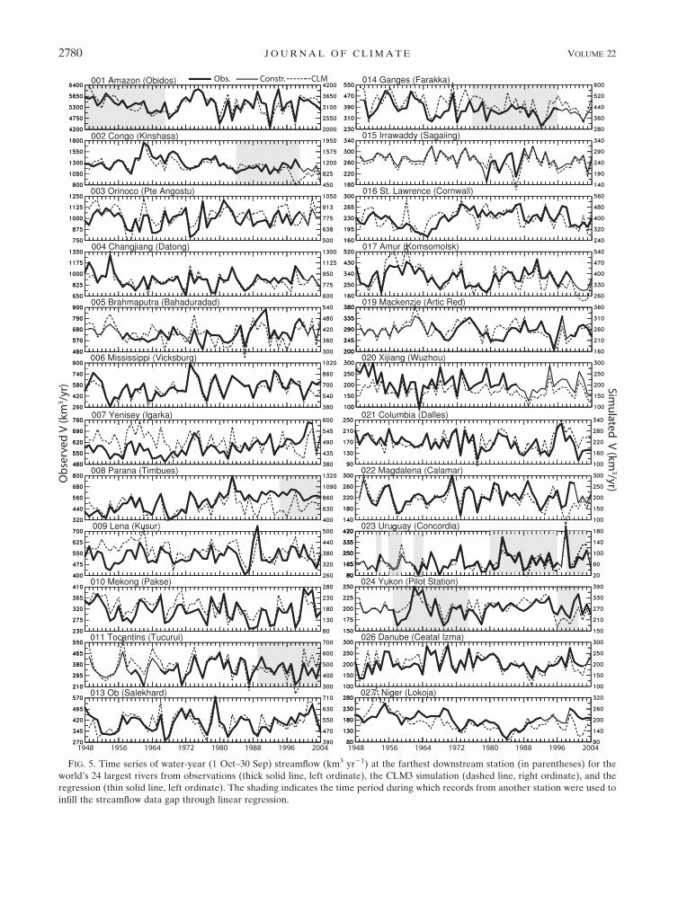
FIG. 5. Time series of water-year (1 Oct–30 Sep) streamflow (km3 yr21) at the farthest downstream station (in parentheses) for the

world’s 24 largest rivers from observations (thick solid line, left ordinate), the CLM3 simulation (dashed line, right ordinate), and the

regression (thin solid line, left ordinate). The shading indicates the time period during which records from another station were used to

infill the streamflow data gap through linear regression.


is superior to pure statistical infilling (such as used by

Labat et al. 2004).

3) ADJUSTMENT TO RIVER MOUTH FLOW

Because our focus is on continental discharge into the

oceans, and the farthest downstream station for many

rivers is often hundreds of kilometers away from the

river mouth, we adjusted the station flow for the world’s

200 largest rivers listed in Dai and Trenberth (2002) to

represent river mouth outflow by multiplying the ob-

served station flow by a ratio of the flow rates at the

river mouth and the station simulated by a river routing

model forced by the observation-based estimates of

runoff fields from Fekete et al. (2002). More informa-

tion is given in Dai and Trenberth (2002).

4) CONTRIBUTIONS FROM UNMONITORED AREAS

To account for the runoff contribution from unmon-

itored areas (or those for which data are unavailable),

which represent about 20% of the global drainage area,

we used the CLM3-simulated runoff field (Qian et al.

2006, 2007) for each year to estimate the annual (for the

water year October–September) discharge using the

following equation (Dai and Trenberth 2002):

R(j) 5 Ro(j)[1 1 r(j) Au(j)/Am(j)] (1)

where R(j) is the continental discharge for 18 latitude

zone j (into individual ocean basins), and Ro(j) is the

contribution from monitored areas (i.e., the sum of river

mouth outflow of all rivers with data within latitude

zone j); Au(j) and Am(j) are the unmonitored and

monitored (by the stations with data) drainage areas,

respectively, whose runoff enters the ocean in latitude

zone j [note: Au(j) and Am(j) may contain land areas

outside zone j]; and r(j) is the ratio of mean runoff (from

the CLM3 simulation) over Au(j) and Am(j) (calculated

for each 48 latitude zone); see Dai and Trenberth (2002)

for details.

3. Results

a. Streamflow trends in the world’s largest rivers

Figure 5 shows the yearly streamflow time series from

1948 to 2004 from observations (thick solid line),

CLM3-based infilling (thin solid line), and CLM3 sim-

ulation for the world’s 24 largest rivers based on ad-

justed river mouth flow. Large multiyear variations are

seen in most of the time series, consistent with previous

analyses (Pekarova et al. 2003). For example, the

Amazon River experienced high flows in the mid-1970s

and low flows in the later 1960s, while the Orinoco had

high flows in the early 1980s and low flows about a de-

cade earlier. Some well-known events are evident in the

streamflow time series. For example, the Sahel drought

during the 1970s and 1980s is reflected by the decreasing

flow in the Niger River, while ENSO influence is ap-

parent over some of the rivers, including lower flows for

the Amazon and higher flows for the Mississippi during

or following El Nino years including 1972–73, 1982–83,

and 1997–98. Other atmospheric modes of variability,

such as the North Atlantic Oscillation and the Pacific

decadal oscillation (PDO), also influence regional pre-

cipitation (Hurrell 1995; Dai et al. 1997) and thus

streamflow around the rims of the North Atlantic and

North Pacific (Brito-Castillo et al. 2003; Milliman et al.

2008). Statistically significant long-term trends [at the

5% level, using the t test described by Woodward and

Gray (1993)] exist during 1948–2004 only for some

of the rivers shown in Fig. 5 (Table 1), namely, the

Congo, Mississippi, Yenisey, Parana, Ganges, Columbia,

Uruguay, and Niger. Because of the relatively short

time period, the linear trends computed are sensitive to

the time period examined. For example, Milliman et al.

(2008) found insignificant trends during 1951–2000 for

the Columbia River.

The CLM3-simulated streamflow generally follows

the observed on both interannual and multidecadal

time scales (Fig. 5), resulting in significant correlations

(Table 1 and Fig. 3), despite the large mean biases for

some of the rivers (e.g., the Uruguay, see Table 1). We

emphasize that the linear regression used in infilling the

data gaps removes any biases and thus it has little effect

on our results here. Figure 5 also shows that the infilling

(thin solid line) of the missing data gaps using the

CLM3-simulated flow through regression is more real-

istic than a zero-anomaly assumption. Furthermore, the

CLM3 was able to capture most of the variations and

long-term changes without considering direct human

influences, such as dam retention and withdrawal of

stream water for irrigation. This suggests that for many

of the world’s large rivers the effects of human activities

on yearly streamflow are likely small compared with

those of climate variations during 1948–2004. This is

consistent with Milliman et al. (2008), who found that

streamflow has decreased more than that implied by

changes in precipitation only over rivers with low

streamflow, such as the Indus, Yellow, and Tigris–

Euphrates. Since the rivers over arid regions contribute

only a very small fraction to the total continental dis-

charge, the direct effects of human activities (besides

through climate change) on continental discharge are

relatively small compared with climate changes. Accu-

mulated over many decades, however, these activities

may still result in nonnegligible effects on the oceanic

water budget (see the introduction).

15 MAY 2009 D A I E T A L . 2781

The linear trends of yearly infilled streamflow for

1948–2004 for the world’s 200 largest rivers are shown in

Fig. 6 as a function of the long-term river flow, with the

statistically significant (at 5% level) trends denoted by

asterisks and insignificant ones by open circles. The

majority of these rivers do not show significant trends

for 1948–2004, although about one-third show signifi-

cant trends of up to 620%–25% of the long-term mean

per decade, and 45 rivers (19 rivers) show negative

(positive) trends. This is qualitatively consistent with

Milliman et al. (2008), who found that out of 34 normal

rivers 24 showed no significant trends during 1951–2000,

and of those with significant trends, more decreased

than increased. (The geographic locations of these river

basins are shown in Fig. 8b.)

There are also other ways to characterize long-term

changes besides linear trends. For example, one can

examine the difference between the mean flow aver-

aged over an earlier and later part of the time period.

Given the large climate shift around 1976–77 associated

with the shift from a cold to warm PDO phase (Trenberth

and Hurrell 1994; Deser et al. 2004), we examined the

composite flow difference between 1948–76 and 1977–

2004. The result (not shown) revealed a smaller number

(23, compared with 64 with significant linear trends) of

the top 200 rivers with significant changes over the two

time periods, further illustrating the sensitivity of the

changes to data periods.

We emphasize that streamflow, like precipitation, has

very large year-to-year variations, which make detec-

tion of changes more difficult. A linear trend is not ex-

pected for any given period but provides one measure

of the change over that period. Hence a ‘‘significant’’

linear trend for 1948–2004 does not imply that this trend

existed before or will continue after this period.

b. Changes in continental discharge

Following Dai and Trenberth (2002), we integrated

the discharge for each 48 latitude 3 58 longitude coastal

box for each individual water year and then computed

the linear trend for each coastal box. Although Fig. 5

suggests that the effect of human activities is likely

secondary compared with climate effects for most of the

world’s large rivers, we did not attempt to exclude any

human-induced changes because our focus is on the

actual flow into the oceans. Because human interference

is likely to decrease flows, increases are more attribut-

able to climatic forcings.

Figure 7 shows the time series of the yearly (October–

September) freshwater discharge into the ocean basins

estimated using the observed streamflow from the 925

rivers with missing data gaps infilled using CLM3-

simulated flow through regression (solid line) and in-

filled using the long-term mean (dashed line). Figure 7 is

designed to show the differences between the two dif-

ferent estimates and does not include the contribution

from the unmonitored areas. Noticeable differences

exist between the estimates using the two infilling

methods, especially for the Indian Ocean, although they

are small because the updated streamflow records are

fairly complete for the majority of the large rivers. Thus,

the conclusions regarding discharge trends in this study

are insensitive to the infilling methods, but this does not

apply to other studies that have more missing data.

Figure 8 shows the water-year discharge trend around

the coasts during 1948–2004 (Fig. 8a) and its implied

runoff trend over the corresponding drainage areas

(Fig. 8b, i.e., by dividing the downstream flow trend with

the upstream drainage area), together with their confi-

dence levels based on the t test (Figs. 8g,h). Here the

gridded coastal discharge trend, which may differ from

the streamflow trend for individual rivers shown in Fig. 5,

was distributed evenly over its drainage area using the

digital river network of Vorosmarty et al. (2000a). Sta-

tistically significant positive trends occur over the

coasts around the Arctic Ocean, especially over eastern

Russia and Canada. Another positive trend is around

the Gulf of Mexico, mainly from the Mississippi River

basin. Decreasing trends over central Africa (mainly

the Congo), West Africa (the Sahel), and southeastern

Australia are statistically significant. On the other hand,

the trends over most South American coasts are insig-

nificant. The magnitude and statistical significance of the

trends are sensitive to the exact time period examined

FIG. 6. Linear trends of yearly streamflow during 1948–2004

plotted as a function of the 1948–2004 mean flow rate of the cor-

responding river. The trend was divided by the long-term mean

and is in percent of the mean per decade, with the statistically

significant trends (at 5% level) denoted by stars and insignificant

ones by open circles [based on the test described in Woodward and

Gray (1993)].


and, in particular, whether the data for the most recent

years are included. For example, the upward trends for

both the Mississippi and Parana leveled off after 1997,

perhaps in response to a subtle shift in the PDO, and

thus analyses with data only up to the late 1990s (e.g.,

Milliman et al. 2008) reveal larger trends than shown here.

To help examine the causes behind the discharge

and runoff trends, Figs. 8c–f show the trends during the

same period in observed surface air temperature and

precipitation [both from Qian et al. (2006)] and CLM3-

simulated snow-cover and soil ice water content. Wide-

spread decreases in precipitation over Africa, southeast-

ern Asia, and eastern Australia coincide with decreased

runoff in these regions, while increases in precipitation

over much of the United States, Argentina, and north-

western Australia are consistent with runoff increases in

these areas. However, the runoff increases over central

and eastern Russia cannot be explained by the de-

creased precipitation (Figs. 8b,d), as noted previously

(Berezovskaya et al. 2004; Milliman et al. 2008). Other

precipitation datasets such as those from the Climate

Research Unit (CRU; http://www.cru.uea.ac.uk/cru/

data/) and the Global Precipitation Climatology Centre

(http://gpcc.dwd.de) show similar trends over these re-

gions. We notice that rain gauge data are sparse in all

precipitation products over many regions such as Siberia,

tropical Africa, and the Amazon and, thus, may contain

large sampling errors. The CLM3 simulation suggests

that large surface warming over Siberia (Fig. 8c) has

caused melting and thus decreases in surface snow cover

(Fig. 8e) and soil ice (Fig. 8f), which can contribute to

increases in runoff. The potential contribution of thawing

of the permafrost, as well as other factors (e.g., changes

in evaporation), to the observed increases in runoff

into the Arctic Ocean has been discussed by Adam and

Lettenmaier (2008).

Figure 9 shows the integrated freshwater discharge

(solid line, including contributions from unmonitored

areas) into the individual and global oceans, together with

an estimate of the uncertainties (shading, cf. section 3).

FIG. 7. Time series of annual (water year) freshwater discharge (in 0.1 Sv; 1 Sv 5 106 m3 s21 5 31.56 3 103 km3 yr21)

from land into the individual and global oceans from 1948 to 2004 estimated using the observed streamflow with data

gaps infilled with CLM3-simulated flow (solid line) and infilled with the long-term mean (dashed line). Runoff from

areas not monitored by the 925 rivers is not accounted for in these estimates (but is included in Figs. 9, 10). Also

shown is the correlation coefficient (r) between the two curves.

15 MAY 2009 D A I E T A L . 2783

Large interannual and decadal variations are evident in

the discharge into all the oceans. Some of these varia-

tions are correlated with the ENSO, as represented by

the Nino-3.4 SST index, which is the normalized sea

surface temperature anomalies averaged over 58S–58N,

1608E–908W [dashed line in Fig. 9, updated from Tren-

berth (1997)] averaged over a 12-month period that leads

the discharge average period by four months for the

Atlantic Ocean (Fig. 9a) and lags the discharge by one

month for the Pacific Ocean (Fig. 9b), by five months for

the Indian Ocean (Fig. 9c), and by one month for the

global ocean as a whole (Fig. 9f). These differences in

the time lag result from the time lag between the index

and ENSO-induced precipitation anomalies, which vary

spatially (Trenberth et al. 2002). The correlation with

the Nino-3.4 SST index is strongest for the Pacific basin

(correlation coefficient r 5 20.61, p , 0.01), as ENSO

greatly affects precipitation over land around the Pacific

rim (Dai and Wigley 2000). El Ninos tend to reduce

streamflow for some Atlantic-draining rivers such as the

Amazon, Orinoco, and Niger, but increase the flow in

rivers such as the Mississippi, Parana, and Uruguay

(cf. Fig. 5), resulting in relatively weak correlation (r 5

20.50, p , 0.01, at the above given lag) between the

Atlantic discharge and the ENSO index (Fig. 9a). Even

for the global discharge, the correlation with ENSO is

fairly strong (r 5 20.66, p , 0.01). No significant cor-

relation is found between ENSO indices and the dis-

charge into the Arctic and the Mediterranean and Black

Seas (Figs. 5d,e), which is not surprising given that the

FIG. 8. Linear trends from 1948 to 2004 in annual (water year) (a) discharge from each 48 lat 3 58 lon coastal box

estimated from available gauge records and reconstructed river flow, (b) the runoff trend inferred from the discharge

trend shown in (a), (c) observed surface air temperature and (d) precipitation (from Qian et al. 2006), and (e) CLM3-

simulated snow cover and soil ice water. The bottom row shows the confidence level (%) for (g) the discharge and (h)

runoff trends based on a t test. A 95% confidence means the trend is statistically significant at the 5% level.


ENSO influence on precipitation is mostly at low and

midlatitudes (Dai and Wigley 2000).

In addition to the large variations, Fig. 9 also shows an

upward trend in the discharge into the Arctic Ocean

(slope b 5 8.2 km3 yr21 or 0.26 3 1023 Sv yr21, p , 0.01)

(Sv [ 106 m3 s21), and downward trends for the Pacific

(b 5 29.4 km3 yr21 or 20.30 3 1023 Sv yr21, p 5 0.01).

Trends in the discharge into the other basins are

negative but statistically insignificant, including the

global oceans as a whole (b 5 26.96 km3 yr21 or

20.23 3 1023 Sv yr21, p 5 0.40). While the increasing

trend in the Arctic discharge is in agreement with

previous reports (Peterson et al. 2002), the negative

trends for the other ocean basins are in sharp contrast

to the perceived but unjustified notion that global

continental discharge should increase as the climate

becomes warmer and the global hydrological cycle in-

tensifies (Milly et al. 2002; Labat et al. 2004; Huntington

2006). On the other hand, the decreasing runoff and

discharge trends are consistent with the trends in the

Palmer drought severity index of the last 50 years or so

(Dai et al. 2004b), which suggests a general drying over

global land.

Precipitation decreases over many of the low- and

midlatitude land areas are the causes for the decline in

runoff during 1948–2004 (Fig. 8). To further illustrate

the relationship with precipitation changes, Fig. 10 com-

pares the drainage-area-integrated precipitation (dashed

line) with the discharge time series (solid line, same as

in Fig. 9). As expected, the discharge time series are sig-

nificantly correlated with precipitation, especially for the

Pacific (r 5 0.62, p , 0.01) on both interannual and longer

FIG. 9. Time series of annual (water year) freshwater discharge (solid line, in 0.1 Sv) from land into the individual and global

oceans from 1948 to 2004. The shading indicates the 6 one standard error, which includes the regression error and the

observational error (estimated as the difference between the observed and the estimated river flow using the regression

equation and CLM-simulated flow). Also shown (dashed, read on the right ordinate) is the Nino-3.4 SST index (Trenberth 1997;

multiplied by 21) averaged over the 12-month period that yields a maximum correlation (r, negative) with the discharge data

(see text for details). The linear slope (b) and its attained significance level [p(b)] of the discharge time series are given on top

of each panel.

15 MAY 2009 D A I E T A L . 2785

time scales, except for the Indian and Arctic Ocean, where

precipitation does not show an upward trend until the

late 1990s (Fig. 10d). The weak correlation for the Indian

Ocean reflects the poor sampling for both streamflow and

precipitation in southern Asia and eastern Africa.

Since the ratio of runoff to precipitation (i.e., the

runoff coefficient) varies from near zero over deserts to

close to one over wet areas, one may expect that mul-

tiplying precipitation by the long-term runoff coefficient

[based on the runoff maps from Fekete et al. (2002) and

precipitation from Qian et al. (2006)] before the area

integration might improve the correlation between

precipitation and the discharge. We found that this is

true only for the relatively dry Mediterranean and Black

Sea drainage basin (r increased from 0.38 to 0.61). For

the other basins, and global land as a whole, the corre-

lation did not change much, suggesting that the runoff

coefficient variations themselves are important.

Extremely high continental discharge occurred in 1974

(Figs. 9 and 10), a La Nina year, and record low discharge

happened in 1992, an El Nino year, for the global and

some of the individual oceans (mainly the Atlantic).

Figure 11 shows the maps of the observed precipitation

and CLM3-simulated runoff anomalies (relative to the

1948–2004 mean) for the water years 1974 and 1992.

Large positive precipitation anomalies occurred in 1974

over Australia, southern and central Africa, tropical

South America, much of the central and eastern United

States and Canada, and north of the Bay of Bengal.

Overall, 1974 was a wet year over most of the continents,

as indicated by the predominant cold colors in Figs. 11a

and 11c. On the other hand, 1992 was an exceptionally

dry year for most of the land areas, especially over the

low latitudes such as the Indonesia–Australia region,

southern Asia, western and southern Africa, tropical

South America, much of Europe, western Canada and the

FIG. 10. Time series of annual (water year) discharge (D, solid line) from 1948 to 2004 compared with observed water-year precipi-

tation [P, dashed line, from Qian et al. (2006)] averaged over the drainage areas of the individual and global oceans. The correlation

coefficients among the two lines are given on top of each panel. The slope (b) and its attained probability ( p) for the discharge are also

shown. For the Arctic drainage basin, another estimate of precipitation [long-dashed line, from CRU_TS_2.10 dataset (Mitchell and

Jones 2005)] is shown.


northwest United States. A regression of the runoff and

precipitation with ENSO indices (Trenberth and Dai

2007) confirms that a large part of these precipitation

anomalies is induced by the cold ENSO event in 1974

and the warm event in 1992. However, the precipitation

and, thus, the discharge and runoff anomalies are also

influenced by other factors, in particular the huge vol-

canic eruption of Mount Pinatubo in June 1991 (Tren-

berth and Dai 2007), as the post-1991 anomalies are more

widespread and larger in magnitude than those associ-

ated with typical ENSO events or even the strongest El

Ninos in 1982 and 1997.

4. Summary and concluding remarks

We have updated the global monthly streamflow

dataset of Dai and Trenberth (2002) with additional

new records for a number of the world’s major rivers.

The average record length for 1948–2004 for the world’s

top 10, 20, 50, 100, and 200 rivers has been improved to

54.2, 42.7, 39.7, and 37.6 yr, respectively, after infilling

data gaps using nearby station data. The remaining data

gaps were infilled with estimates derived using the

CLM3-simulated streamflow through regression, which

makes use of precipitation data and the correlation

between precipitation and streamflow. This has resulted

in a new global dataset of continuous monthly stream-

flow from 1948 to 2004 at the farthest downstream sta-

tions for the world’s 925 largest ocean-reaching rivers.

This network of gauges covers ;80 3 106 km2 or ;80%

of global ocean-draining areas and accounts for about

73% of global total runoff, although some data gaps

(before the infilling) exist for many of the gauge rec-

ords, which reduces the coverage for some individual

years.

The CLM3-simulated runoff ratio [cf. Eq. (1)] was

used to estimate the contribution from the drainage

areas not monitored by the 925 rivers, whereas the ratio

of the simulated flow at the river mouth and the farthest

downstream station by a river routing model forced with

observation-based long-term runoff fields (from Fekete

et al. 2002) was used to adjust the station flow to rep-

resent river mouth outflow. Therefore, our estimates of

the continental discharge include runoff from all land

areas except Antarctica [;2613 km3 yr21 according to

Jacobs et al. (1992)] and Greenland. There is also a

small coastal discharge through groundwater [estimated

as 2200 km3 yr21 globally by Korzun et al. (1977)], al-

though part of this groundwater discharge is included

in our estimates of the discharge contribution from

the unmonitored areas because the groundwater has to

come from surface (runoff) water on a long-term basis.

For comparison, our estimate of long-term global dis-

charge is about 37 288 km3 yr21 or 1.18 Sv [see Table 4

of Dai and Trenberth (2002), excluding Antarctica and

Greenland].

FIG. 11. (top) Observed precipitation and (bottom) CLM3-simulated runoff anomalies (in mm day21, relative to

1948–2004 mean) for the water year (left) 1974 and (right) 1992.

15 MAY 2009 D A I E T A L . 2787

Although our dataset contains records before 1948

and up to 2006 for many rivers, our analysis here fo-

cused on the 1948–2004 period when the record is most

complete for the majority of the rivers. Comparisons

with the CLM3-simulated streamflow, which does not

include any direct human influence (other than through

human-induced climate changes), suggest that for most

of the world’s large rivers the effect of the human ac-

tivities on yearly streamflow (including its trend) are

likely small compared with that of climate changes since

1948 (but human activities do have other impacts, see

the introduction). Consistent with previous analyses,

large interannual to decadal variations are seen in the

streamflow in most of the world’s major rivers. How-

ever, statistically significant trends up to 620%–25%

per decade during 1948–2004 exist only for about one-

third of the world’s top 200 rivers, including the Congo,

Mississippi, Yenisey, Parana, Ganges, Columbia,

Uruguay, and Niger, with the rivers having downward

trends (45) outnumbering those with upward trends

(19). The magnitude and statistical significance of the

trends are sensitive to the time period examined.

Large interannual to decadal variations in conti-

nental discharge are correlated with ENSO events for

the discharge into the Atlantic, Pacific, Indian, and

global oceans as a whole, but not with discharges into

the Arctic Ocean and the Mediterranean and Black

Seas, suggesting that ENSO-induced precipitation anom-

alies over the low- and midlatitude land areas are a

major cause for the variations in continental discharge,

consistent with many regional analyses (e.g., Kahya and

Dracup 1993; Pasquini and Depetris 2007) and precip-

itation analyses (Dai and Wigley 2000; Gu et al. 2007).

Consistent with previous reports, we found a large

upward trend in the yearly discharge into the Arctic

Ocean (8.2 km3 yr21) from 1948 to 2004. For the other

ocean basins and the global oceans as a whole, the

discharge has downward trends, which are statistically

significant for the Pacific (29.4 km3 yr21). Aside from

the Arctic and Indian Oceans, where precipitation data

contain large uncertainties, precipitation is significantly

correlated with discharge, suggesting that precipitation

change is a major cause for the discharge trends and large

interannual to decadal variations. Seasonal trends are

not examined here as they are more susceptible to non-

climatic effects such as dams, reservoirs and irrigation,

which makes their interpretation more difficult.

Our results are consistent with the widespread drying

during recent decades over global land found by Dai

et al. (2004b). They are also consistent with the insig-

nificant trend in global discharge during 1951–2000

found by Milliman et al. (2008). However, our results

contradict the notion that global runoff has increased

during recent decades (Labat et al. 2004) and that en-

hanced water use efficiency by plants has contributed to

the runoff increase (Gedney et al. 2006) (see appendix B

for more details on these two studies). Multimodel en-

semble predictions by current climate models show

consistent increases in streamflow only for the northern

high-latitude rivers (Nohara et al. 2006) because pro-

jected precipitation changes are far from uniform in-

creases; there are widespread decreases in the sub-

tropics (e.g., Dai et al. 2001; Sun et al. 2007; Solomon

et al. 2007). The downward trends in low- and midlati-

tude streamflow records are consistent with the general

drying trend over global land during the last 50 years or

so (Dai et al. 2004b).

The reduced runoff in low and midlatitudes has in-

creased the pressure on limited freshwater resources

over the world, especially as the demand increases with

the world’s population growth (Vorosmarty et al. 2000b).

This problem is likely to continue or even worsen in the

coming decades based on the multimodel predictions of

precipitation and streamflow of the twenty-first century

(Solomon et al. 2007).

Acknowledgments. This study was partly supported

by NSF Grant ATM-0233568 and NCAR’s Water Cycle

Program. The streamflow dataset will be freely avail-

able from http://www.cgd.ucar.edu/cas/catalog/ after the

publication of this paper.

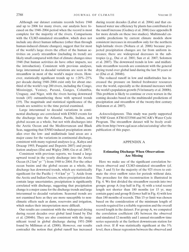
APPENDIX A

Estimating Discharge When ObservationsAre Missing

Here we make use of the significant correlation be-

tween observed and CLM3-simulated streamflow (cf.

Figs. 3 and 5) for the majority of the 925 rivers to esti-

mate the river outflow rates for periods without data.

The procedure for this reconstruction is illustrated in

Fig. 4. We first divided the streamflow records into two

groups: group A (top half in Fig. 4) with a total record

length not shorter than 180 months (or 15 yr, may

contain gaps) and group B (lower half in Fig. 4) with less

than 180 months of records. This 15-yr limit was chosen

based on the consideration of the minimum length of

records required for a reliable regression and the overall

record length in the dataset. For group A, we computed

the correlation coefficient (R) between the observed

and simulated 12 monthly and 1 annual streamflow time

series separately at the farthest downstream station for

each river. If R was statistically significant at the 5%

level, then a linear regression between the observed and


simulated streamflow time series (for each month and

the annual mean) was used to derive streamflow rates

for the months without data using the simulated flow as

input (annual values were estimated using the annual

regression). When the correlation for some monthly

time series was insignificant but there were 8 or more

other months with significant correlation and valid re-

gression, then data gaps in those monthly time series

without regression were filled using spline interpolation

of observed or estimated streamflow of the other

months. As shown in Fig. 4, there were about 419 (or

45%) rivers whose annual and monthly streamflow time

series were significantly correlated with the CLM3-

simulated flow for at least 8 or more of the 12 months.

For the remaining rivers in group A (i.e., those did not

fit into categories c00 and c01 in Fig. 4), a correlation

(Ram) using the 12-month-combined time series of

streamflow from the observations and the CLM3 sim-

ulation was computed. If Ram was significant at the 5%

level, then a regression between the all-month time se-

ries was used to fill the missing monthly gaps. Annual

values were derived from annual regression in this case,

that is, c02 in Fig. 4. If Ram was insignificant at zero lag

but became significant and maximized when we intro-

duced a time lag from 25 to 15 months, then a re-

gression was done at that lag and used to fill the monthly

data gaps (c03). Categories c02 and c03 were repeated

for those rivers in group A whose annual time series

were not significantly correlated (c05 and c06).

About 27.6% of the rivers fell into group B, with a

record shorter than 180 months. For this group, the

correlation and regression were done for 12-month-

combined time series only (with the annual cycle in-

cluded). If the simultaneous correlation was significant,

then a regression was used to fill the monthly gaps

(c08, 25.8%); otherwise, the maximum lag correlation

(within 65 months) was sought and a regression was

used to fill the monthly data gaps if the maximum lag

correlation was significant (c09, 1.2%). Annual values

were derived from the monthly data or estimates for

rivers in group B. We realize that inclusion of the an-

nual cycle for group B rivers may enhance the corre-

lation; however, we do not think it has significant ef-

fects on the discharge estimates because these are mostly

small rivers.

APPENDIX B

Reasons for Different Findings by Previous Studies

Here we explore why Labat et al. (2004) reached

different conclusions. Labat et al. (2004) obtained

monthly streamflow data for 221 rivers from the

GRDC and another source (for the Amazon only),

which account for about half of the global discharge

for years when all of the rivers have observations.

However, they used only 10 so-called reference rivers

for reconstruction of the complete time series from

1880 to 1925 and considered the variations only at

monthly, annual, and multiyear time scales during the

reconstruction through a wavelet transform so that

decadal and longer variations were excluded. Global

discharge time series were derived by summing up

these 10 time series, and a constant, scaling coeffi-

cient was used to account for the complete conti-

nental surface. This scaling coefficient was derived

from the outdated long-term mean global and conti-

nental discharge estimates by Baumgartner and

Reichel (1975) [see Dai and Trenberth (2002) for

problems in the Baumgartner and Reichel estimates].

Finally, the estimate was scaled up by a factor of

1/0.89 to account for the contribution from Australia

and Antarctica. In essence, the variations and trends

in the global discharge time series of Labat et al.

(2004) were derived completely from streamflow

records of only 10 rivers with constant scaling for the

1880–1925 period, and their conclusion was based on

the trend estimated for the entire 1880–1994 period.

Our experience with the available streamflow records

suggests that it is very difficult, if not impossible, to

derive reliable estimates of global continental dis-

charge for decades before the 1940s simply because

most of the world’s major rivers do not have obser-

vations during the first half of the twentieth century

(let alone the nineteenth century). Hence, our esti-

mate of discharge trends for 1948–2004 is not com-

parable with the Labat et al. (2004) estimate for

;1875–1994.

Gedney et al. (2006) first accepted the discharge in-

crease reported by Labat et al. (2004) as the truth and

applied a land surface model, similar to the CLM3,

forced with Climate Research Unit monthly surface

data, which included climatological values for many

land areas, and climatological winds to attribute the

discharge increases to several factors. They concluded

that enhanced water use efficiency by plants is a big

contributor to the runoff increase. Neither our CLM3

simulation, which is very similar to the model simula-

tions done by Gedney et al. (2006) except we used a

different forcing dataset, nor our analysis of the stream-

flow records show significant upward trends in global

discharge during the last five decades when atmospheric

CO2 has been steadily increasing. This suggests that the

conclusion of Gedney et al. (2006) is model and data

dependent.

15 MAY 2009 D A I E T A L . 2789

REFERENCES

Adam, J. C., and D. P. Lettenmaier, 2008: Application of new

precipitation and reconstructed streamflow products to

streamflow trend attribution in northern Eurasia. J. Climate,

21, 1807–1828.

Baumgartner, A., and E. Reichel, 1975: The World Water Balance.

Elsevier, 179 pp.

Berezovskaya, S., D. Yang, and D. L. Kane, 2004: Compatibility

analysis of precipitation and runoff trends over the large Sibe-

rian watersheds. Geophys. Res. Lett., 31, L21502, doi:10.1029/

2004GL021277.

Betts, A. K., J. H. Ball, P. Viterbo, A. G. Dai, and J. Marengo,

2005: Hydrometeorology of the Amazon in ERA-40.

J. Hydrometeor., 6, 764–774.

Birsan, M. V., P. Molnar, P. Burlando, and M. Pfaundler, 2005:

Streamflow trends in Switzerland. J. Hydrol., 314, 312–329.

Bodo, B. A., 2001: Annotations for monthly discharge data for world

rivers (excluding former Soviet Union). Version 1.3, 111 pp.

[Available online at http://dss.ucar.edu/datasets/ds552.1/docs/

docglob.pdf.]

Boyer, E. W., R. W. Howarth, J. N. Galloway, F. J. Dentener, P. A.

Green, and C. J. Vorosmarty, 2006: Riverine nitrogen export

from the continents to the coasts. Global Biogeochem. Cycles,

20, GB1S91, doi:10.1029/2005GB002537.

Brito-Castillo, L., A. V. Douglas, A. Leyva-Contreras, and

D. Lluch-Belda, 2003: The effect of large-scale circulation

on precipitation and streamflow in the Gulf of California

continental watershed. Int. J. Climatol., 23, 751–768.

Callede, J., J. L. Guyot, J. Ronchail, M. Molinier, and E. De Oliveira,

2002: The River Amazon at Obidos (Brazil): Statistical

studies of the discharges and water balance. Hydrol. Sci. J.,

47, 321–333.

Carton, J. A., 1991: Effect of seasonal surface fresh-water flux on

sea surface temperature in the tropical Atlantic Ocean.

J. Geophys. Res., 96, 12 593–12 598.

Cayan, D. R., S. A. Kammerdiener, M. D. Dettinger, J. M.

Caprio, and D. H. Peterson, 2001: Changes in the onset of

spring in the western United States. Bull. Amer. Meteor.

Soc., 82, 399–415.

Cazenave, A., F. Remy, K. Dominh, and H. Douville, 2000: Global

ocean mass variation, continental hydrology and the mass

balance of Antarctica ice sheet at seasonal time scale. Geo-

phys. Res. Lett., 27, 3755–3758.

Chao, B. F., Y. H. Wu, and Y. S. Li, 2008: Impact of artificial

reservoir water impoundment on global sea level. Science,

320, 212–214.

Cluis, D., and C. Laberge, 2001: Climate change and trend detec-

tion in selected rivers within the Asia-Pacific region. Water

Int., 26, 411–424.

Cowell, C. M., and R. T. Stoudt, 2002: Dam-induced modifications

to upper Allegheny River streamflow patterns and their biodi-

versity implications. J. Amer. Water Resour. Assoc., 38, 187–196.

Crow, E. L., F. A. Davis, and M. W. Maxfield, 1960: Statistics

Manual. Dover, 288 pp.

Dai, A., and I. Fung, 1993: Can climate variability contribute

to the ‘‘missing’’ CO2 sink? Global Biogeochem. Cycles, 7,

599–609.

——, and T. M. L. Wigley, 2000: Global patterns of ENSO-

induced precipitation. Geophys. Res. Lett., 27, 1283–1286.

——, and K. E. Trenberth, 2002: Estimates of freshwater dis-

charge from continents: Latitudinal and seasonal variations.


——, I. Y. Fung, and A. D. Del Genio, 1997: Surface observed

global land precipitation variations during 1900–88. J. Climate,

10, 2943–2962.

——, T. M. L. Wigley, B. A. Boville, J. T. Kiehl, and L. E. Buja,

2001: Climates of the 20th and 21st centuries simulated by the

NCAR Climate System Model. J. Climate, 14, 485–519.

——, P. J. Lamb, K. E. Trenberth, M. Hulme, P. D. Jones, and

P. Xie, 2004a: The recent Sahel drought is real. Int. J. Climatol.,

24, 1323–1331.

——, K. E. Trenberth, and T. T. Qian, 2004b: A global dataset of

Palmer Drought Severity Index for 1870–2002: Relationship

with soil moisture and effects of surface warming. J. Hydro-

meteor., 5, 1117–1130.

Deser, C., A. S. Phillips, and J. W. Hurrell, 2004: Pacific interdecadal

climate variability: Linkages between the tropics and the North

Pacific during boreal winter since 1900. J. Climate, 17, 3109–3124.

Dettinger, M. D., and H. F. Diaz, 2000: Global characteristics of

stream flow seasonality and variability. J. Hydrometeor., 1,

289–310.

Domingues, C. M., J. A. Church, N. J. White, P. J. Gleckler, S. E.

Wijffels, P. M. Barker, and J. R. Dunn, 2008: Improved esti-

mates of upper-ocean warming and multi-decadal sea-level

rise. Nature, 453, 1090–1093.

Fekete, B. M., C. J. Vorosmarty, and W. Grabs, 2000: Global

composite runoff fields based on observed river discharge and

simulated water balances. Global Runoff Data Centre Rep.

22, 39 pp. [Available online at http://grdc.bafg.de/servlet/is/

911/Report22.pdf?command5downloadContent&filename5

Report22.pdf.]

——, ——, and ——, 2002: High-resolution fields of global runoff

combining observed river discharge and simulated water

balances. Global Biogeochem. Cycles, 16, 1042, doi:10.1029/

1999GB001254.

Gedney, N., P. M. Cox, R. A. Betts, O. Boucher, C. Huntingford,

and P. A. Stott, 2006: Detection of a direct carbon dioxide effect

in continental river runoff records. Nature, 439, 835–838.

Genta, J. L., G. Perez-Iribarren, and C. R. Mechoso, 1998: A re-

cent increasing trend in the streamflow of rivers in south-

eastern South America. J. Climate, 11, 2858–2862.

Grabs, W. E., T. de Couet, and J. Pauler, 1996: Freshwater fluxes

from continents into the world oceans based on data of the

Global Runoff Data Base. Global Runoff Data Centre Rep.

10, 49 pp. [Available from GRDC, Federal Institute of Hy-

drology, Am Mainzer Tor 1, 56068 Koblenz, Germany.]

——, F. Portmann, and T. de Couet, 2000: Discharge observation

networks in Arctic regions: Computation of the river runoff

into the Arctic Ocean, its seasonality and variability. The

Freshwater Budget of the Arctic Ocean, E. L. Lewis et al., Eds.,

Kluwer Academic, 249–267.

Groisman, P. Ya., R. W. Knight, and T. R. Karl, 2001: Heavy

precipitation and high streamflow in the contiguous United

States: Trends in the twentieth century. Bull. Amer. Meteor.

Soc., 82, 219–246.

Gu, G., R. F. Adler, G. J. Huffman, and S. Curtis, 2007: Tropical

rainfall variability on interannual-to-interdecadal longer time

scales derived from the GPCP monthly product. J. Climate,

20, 4033–4066.

Guetter, A. K., and K. P. Georgakakos, 1993: River outflow of the

conterminous United States, 1939–1988. Bull. Amer. Meteor.

Soc., 74, 1873–1891.

Hodgkins, G. A., R. W. Dudley, and T. G. Huntington, 2003:

Changes in the timing of high river flows in New England over

the 20th century. J. Hydrol., 278, 244–252.


Huntington, T. G., 2006: Evidence for intensification of the

global water cycle: Review and synthesis. J. Hydrol., 319,

83–95.

Hurrell, J. W., 1995: Decadal trends in the North Atlantic Oscil-

lation: Regional temperatures and precipitation. Science, 269,

676–679.

Hyvarinen, V., 2003: Trends and characteristics of hydrological

time series in Finland. Nord. Hydrol., 34, 71–90.

Jacobs, S. S., H. H. Helmer, C. S. M. Doake, A. Jenkins, and R. M.

Frolich, 1992: Melting of ice shelves and the mass balance of

Antarctica. J. Glaciol., 38, 375–387.

Kahya, E., and J. A. Dracup, 1993: United States streamflow

patterns in relation to the El Nino/Southern Oscillation.

Water Resour. Res., 29, 2491–2503.

Korzun, V. I., A. A. Sokolov, M. I. Budyko, K. P. Voskrensensky,

G. P. Kalinin, A. A. Konoplyantsev, E. S. Korotkevich, and

M. I. Lvovich, 1977: Atlas of the World Water Balance.

UNESCO, 36 pp.

Krepper, C. M., N. O. Garcıa, and P. D. Jones, 2006: Paraguay

River basin response to seasonal rainfall. Int. J. Climatol., 26,

1267–1278.

Labat, D., Y. Godderis, J. L. Probst, and J. L. Guyot, 2004: Evi-

dence for global runoff increase related to climate warming.

Adv. Water Resour., 27, 631–642.

Lammers, R. B., A. I. Shiklomanov, C. J. Vorosmarty, B. M.

Fekete, and B. J. Peterson, 2001: Assessment of contemporary

Arctic river runoff based on observational discharge records.

J. Geophys. Res., 106, 3321–3334.

Legates, D. R., H. F. Lins, and G. J. McCabe, 2005: Comments

on ‘‘Evidence for global runoff increase related to climate

warming’’ by Labat et al. Adv. Water Resour., 28, 1310–1315.

Lettenmaier, D. P., E. F. Wood, and J. R. Wallis, 1994: Hydro-

climatological trends in the continental United States, 1948–88.

J. Climate, 7, 586–607.

Lindstrom, G., and S. Bergstrom, 2004: Runoff trends in Sweden

1807–2002. Hydrol. Sci. J., 49, 69–83.

Lins, H. F., and J. R. Slack, 1999: Streamflow trends in the United

States. Geophys. Res. Lett., 26, 227–230.

Marcinek, J., 1964: The river discharge from land surface over the

globe and its distribution in 58 zones (in German). Mitteilungen

des Institutes fuer Wasserwirtschaft Tech. Rep. 21, 204 pp.

Milliman, J. D., K. L. Farnsworth, P. D. Jones, K. H. Xu, and L. C.

Smith, 2008: Climatic and anthropogenic factors affecting

river discharge to the global ocean, 1951–2000. Global Planet.

Change, 62, 187–194.

Milly, P. C. D., R. T. Wetherald, K. A. Dunne, and T. L. Delworth,

2002: Increasing risk of great floods in a changing climate.

Nature, 415, 514–517.

Mitchell, T. D., and P. D. Jones, 2005: An improved method of

constructing a database of monthly climate observations and

associated high-resolution grids. Int. J. Climatol., 25, 693–712.

Ngo-Duc, T., K. Laval, J. Polcher, A. Lombard, and A. Cazenave,

2005: Effects of land water storage on global mean sea level

over the past half century. Geophys. Res. Lett., 32, L09704,

doi:10.1029/2005GL022719.

Nilsson, C., C. A. Reidy, M. Dynesius, and C. Revenga, 2005:

Fragmentation and flow regulation of the world’s large river

systems. Science, 308, 405–408.

Nohara, D., A. Kitoh, M. Hosaka, and T. Oki, 2006: Impact of

climate change on river discharge projected by multimodel

ensemble. J. Hydrometeor., 7, 1076–1089.

Oki, T., and S. Kanae, 2006: Global hydrological cycles and world

water resources. Science, 313, 1068–1072.

Oleson, K. W., and Coauthors, 2004: Technical description of the

Community Land Model (CLM). NCAR Tech. Note NCAR/

TN-4611STR, 186 pp.

Pasquini, A. I., and P. J. Depetris, 2007: Discharge trends and

flow dynamics of South American rivers draining the

southern Atlantic seaboard: An overview. J. Hydrol., 333,

385–399.

Peel, M. C., and T. A. McMahon, 2006: Continental runoff: A

quality-controlled global runoff data set. Nature, 444, E14.

Pekarova, P., P. Miklanek, and J. Pekar, 2003: Spatial and

temporal runoff oscillation analysis of the main rivers of

the world during the 19th–20th centuries. J. Hydrol., 274,

62–79.

Perry, G. D., P. B. Duffy, and N. L. Miller, 1996: An extended data

set of river discharges for validation of general circulation

models. J. Geophys. Res., 101, 21 339–21 349.

Peterson, B. J., R. M. Holmes, J. W. McClelland, C. J. Vorosmarty,

R. B. Lammers, A. I. Shiklomanov, I. A. Shiklomanov, and

S. Rahmstorf, 2002: Increasing river discharge to the Arctic

Ocean. Science, 298, 2171–2173.

Probst, J. L., and Y. Tardy, 1987: Long-range streamflow and world

continental runoff fluctuations since the beginning of this

century. J. Hydrol., 94, 289–311.

——, and ——, 1989: Global runoff fluctuations during the last 80

years in relation to world temperature change. Amer. J. Sci.,

289, 267–285.

Qian, T., A. Dai, K. E. Trenberth, and K. W. Oleson, 2006: Sim-

ulation of global land surface conditions from 1948–2004. Part I:

Forcing data and evaluation. J. Hydrometeor., 7, 953–975.

——, ——, and ——, 2007: Hydroclimatic trends in the Mississippi

River basin from 1948–2004. J. Climate, 20, 4599–4614.

Robson, A. J., 2002: Evidence for trends in UK flooding. Phil.

Trans. Roy. Soc. London, 360A, 1327–1343.

Shiklomanov, A. I., T. I. Yakovleva, R. B. Lammers, I. P. Karasev,

C. J. Vorosmarty, and E. Linder, 2006: Cold region river

discharge uncertainty—Estimates from large Russian rivers.

J. Hydrol., 326, 231–256.

Smith, L. C., 2000: Trends in Russian Arctic river-ice formation

and breakup: 1917 to 1994. Phys. Geogr., 21, 46–56.

Solomon, S., D. Qin, M. Manning, M. Marquis, K. Averyt, M. M. B.

Tignor, H. L. Miller Jr., and Z. Chen, Eds., 2007: Climate

Change 2007: The Physical Science Basis. Cambridge University

Press, 996 pp.

Sun, Y., S. Solomon, A. Dai, and R. Portmann, 2007: How often

will it rain? J. Climate, 20, 4801–4818.

Trenberth, K. E., 1997: The definition of El Nino. Bull. Amer.

Meteor. Soc., 78, 2771–2777.

——, and J. W. Hurrell, 1994: Decadal atmosphere-ocean varia-

tions in the Pacific. Climate Dyn., 9, 303–319.

——, and A. Dai, 2007: Effects of Mount Pinatubo volcanic erup-

tion on the hydrological cycle as an analog of geoengineering.

Geophys. Res. Lett., 34, L15702, doi:10.1029/2007GL030524.

——, J. M. Caron, D. P. Stepaniak, and S. Worley, 2002: Evolution

of El Nino–Southern Oscillation and global atmospheric

surface temperatures. J. Geophys. Res., 107, 4065, doi:10.1029/

2000JD000298.

——, L. Smith, T. Qian, A. Dai, and J. Fasullo, 2007: Estimates of

the global water budget and its annual cycle using observational

and model data. J. Hydrometeor., 8, 758–769.

Vorosmarty, C. J., B. M. Fekete, M. Meybeck, and R. B. Lammers,

2000a: Global system of rivers: Its role in organizing conti-

nental land mass and defining land-to-ocean linkages. Global

Biogeochem. Cycles, 14, 599–621.

15 MAY 2009 D A I E T A L . 2791

——, P. Green, J. Salisbury, and R. B. Lammers, 2000b: Global

water resources: Vulnerability from climate change and popula-

tion growth. Science, 289, 284–288.

Woodward, W. A., and H. L. Gray, 1993: Global warming and the

problem of testing for trend in time series data. J. Climate, 6,

953–962.

Xiong, L. H., and S. L. Guo, 2004: Trend test and change-

point detection for the annual discharge series of the Yangtze

River at the Yichang hydrological station. Hydrol. Sci. J., 49,

99–112.

Yang, D., B. Ye, and D. L. Kane, 2004a: Streamflow changes over

Siberian Yenisei River basin. J. Hydrol., 296, 59–80.

——, ——, and A. Shiklomanov, 2004b: Discharge characteris-

tics and changes over the Ob River watershed in Siberia.


Ye, B., D. Yang, and D. L. Kane, 2003: Changes in Lena River

streamflow hydrology: Human impacts versus natural varia-

tions. Water Resour. Res., 39, 1200, doi:10.1029/2003WR001991.

Zhang, X., K. D. Harvey, W. D. Hogg, and T. R. Yuzyk, 2001:

Trends in Canadian streamflow. Water Resour. Res., 37, 987–998.


changes in continental freshwater discharge from … in continental freshwater discharge from 1948...

Documents