changes in the federal reserve communication strategy · pdf filechanges in the federal...

No.11-E-2 March 2011

Changes in the Federal Reserve Communication Strategy: A Structural Investigation Yasuo Hirose* [email protected] Takushi Kurozumi** [email protected]

Bank of Japan 2-1-1 Nihonbashi Hongoku-cho, Chuo-ku, Tokyo 103-8660

* Faculty of Economics, Keio University. ** Monetary Affairs Department, Bank of Japan. Papers in the Bank of Japan Working Paper Series are circulated in order to stimulate discussion and comments. Views expressed are those of authors and do not necessarily reflect those of the Bank. If you have any comment or question on the working paper series, please contact each author. When making a copy or reproduction of the content for commercial purposes, please contact the Public Relations Department ([email protected]) at the Bank in advance to request permission. When making a copy or reproduction, the source, Bank of Japan Working Paper Series, should explicitly be credited.

Bank of Japan Working Paper Series

Changes in the Federal Reserve Communication Strategy:

A Structural Investigation�

Yasuo Hirosey Takushi Kurozumiz

This version: March 2011

Abstract

This paper structurally investigates the changes in the Federal Reserve�s communication

strategy during the 1990s by analyzing anticipated and unanticipated disturbances to a

Taylor rule. The anticipated monetary policy disturbances are identi�ed by estimating

a medium-scale dynamic stochastic general equilibrium model with the term structure of

interest rates, using the U.S. data that includes bond yields. The estimation results show

that the Fed made its future policy actions unanticipated for market participants until the

mid-1990s, but thereafter, the Fed tended to coordinate market expectations about future

policy actions. This �nding suggests that the changes in the Fed�s communication strategy

are consistent with the rise of the academic views on central banking as management of

expectations. The inclusion of bond yields in the data for estimation is indispensable to

the �nding because the yields contain crucial information on the expected future path of

the federal funds rate. Moreover, it is demonstrated that the presence of bond yields data

generates a substantial contribution of monetary policy disturbances to business cycles.

Keywords: Monetary policy disturbance, Central bank communication, Management of

expectations, Term structure of interest rates, Federal Reserve

JEL Classi�cation: E52, E58

�The authors are grateful for comments and discussions to Masayoshi Amamiya, Kosuke Aoki, Hiroshi Fujiki,

Ippei Fujiwara, Marvin Goodfriend, Hibiki Ichiue, Hirokazu Ishise, Ryo Kato, Takeshi Kato, Kentaro Koyama,

Shigeki Kushida, Nobuyuki Oda, Shinsuke Ohyama, Toshitaka Sekine, Mototsugu Shintani, Shigenori Shiratsuka,

Kazuo Ueda, and Kozo Ueda, as well as participants at the IMES Brown Bag Seminar. Any remaining errors

are the sole responsibility of the authors. The views expressed herein are those of the authors and should not

be interpreted as those of the Bank of Japan.

yFaculty of Economics, Keio University. E-mail address: [email protected]

zMonetary A¤airs Department, Bank of Japan. E-mail address: [email protected]

1

1 Introduction

Since the seminal work by Taylor (1993), the U.S. monetary policy has been studied with an

estimated policy rule for the federal funds rate (e.g., Clarida, Galí, and Gertler, 1998, 2000;

Judd and Rudebusch, 1998; Orphanides, 2001, 2002, 2003; Taylor, 1999).1 This policy rule

serves as a useful description of the Federal Reserve�s adjustment of the federal funds rate,

and decomposes this rate to a rule-based component and a disturbance. While the rule-based

component represents the Fed�s systematic adjustment of the rate for its target variables (e.g.,

in�ation), the disturbance is regarded as the Fed�s discretion constrained in the presence of the

systematic adjustment (Bernanke, 2003).

In the existing literature, the disturbances to monetary policy rules have been called mon-

etary policy shocks, since it is typically assumed that the disturbances are unanticipated for

private agents. However, not all monetary policy disturbances are unanticipated. Some are

anticipated through the Fed�s communications. The statement of the Federal Open Market

Committee (FOMC) in August 2003, for instance, announced �the Committee believes that

policy accommodation can be maintained for a considerable period.�Moreover, in June 2004,

when the Fed started to raise the target rate for the federal funds at a measured pace, the

FOMC statement included the sentence �the Committee believes that policy accommodation

can be removed at a pace that is likely to be measured.�These statements have a coordination

e¤ect on �nancial market expectations about the future path of the federal funds rate, and it

can be considered that this e¤ect arises from an anticipated future monetary policy disturbance

that captures the Fed�s management of expectations.

This paper structurally identi�es the anticipated and unanticipated components of the

monetary policy disturbances to investigate the changes in the Fed�s communication strategy

during the 1990s.2 The Fed decided in 1994 to release a statement describing policy actions

on the federal funds rate at the conclusion of any FOMC meeting at which a policy action was

undertaken, and determined in 1999 to issue a statement reporting the settings of the target rate

for the federal funds and the balance of risks to the Fed�s objectives after every FOMC meeting.

Our strategy for the identi�cation of anticipated future monetary policy disturbances is based

1The role of the federal funds rate as the Fed�s key policy instrument was established by Goodfriend (1991).

2Blinder et al. (2001) indicate that the Fed has changed its communication strategy dramatically since 1993

and that the Fed�s attitudes toward communication changed between 1995 and 1999.

2

on the idea that the e¤ects of these decisions regarding the Fed�s communication strategy are

contained in the �nancial market data. In this context, Blinder et al. (2001) indicate that,

during the period from early 1996 to mid-1999, the U.S. bond market moved in response to

the macroeconomic developments that helped to stabilize the U.S. economy, despite relatively

little change in the current level of the federal funds rate. As Blinder et al. argue, this re�ects

an improvement in the �nancial market�s ability to forecast the Fed�s future policy actions.

We thus include the U.S. Treasury bond yields, which contain information on the future path

of the federal funds rate expected by the market participants, in the data for the estimation

of a Taylor rule together with the term structure of interest rates, which relates the bond

yields to the federal funds rate. More speci�cally, anticipated and unanticipated components

of disturbances to the Taylor rule are identi�ed by the Bayesian estimation of a version of

Smets and Wouters�(2007) model incorporated with the term structure, using the bond yields

data as well as other macroeconomic data.3

The estimation results show that a large fraction of the anticipated component of distur-

bances to the Taylor rule was not met until the mid-1990s, but thereafter, this component

tended to materialize. Moreover, the variance decompositions of the monetary policy distur-

bances in two subsamples, before and after the mid-1990s, show that the contribution of the

anticipated component to the whole policy disturbances became larger after the mid-1990s.

These results imply that the Fed made its future policy actions unanticipated for market par-

ticipants until the mid-1990s, but thereafter, the Fed tended to coordinate �nancial market

expectations about future policy actions. Furthermore, it is demonstrated that the inclusion

of bond yields in the data for estimation is indispensable to these results. Exclusion of the

bond yields data results in no signi�cant di¤erence between the periods before and after the

mid-1990s in the estimated series of the anticipated and unanticipated components of the policy

disturbances.

The main �nding of the Fed�s coordinating future policy expectations after the mid-1990s

suggests that the changes in the Fed�s communication strategy are consistent with the rise of

the academic views on central banking as management of expectations. As Goodfriend (2010)

points out, the Fed in the mid-1990s was inclined to communicate to �nancial markets in terms

3De Graeve, Emiris, and Wouters (2009) empirically demonstrate that a variant of Smets and Wouters�(2007)

model combined with the term structure of interest rates can well explain the movements in the U.S. yield curve.

3

of interest rate policy, since academic literature had developed indicating that communication

could enhance the e¤ectiveness of the policy. In this context, Woodford (2001, 2003, 2005)

stresses that better information on the part of �nancial market participants about central

banks� actions and intensions increases the degree to which the banks� policy decisions can

actually in�uence market expectations about future policy actions, and thus improves the

monetary policy e¤ectiveness. Moreover, Blinder et al. (2008) emphasize the role of �news�

or �signals� by central banks for the management of expectations. The anticipated future

monetary policy disturbances examined in the present paper can be regarded as a form of such

news or signals by the Fed.

This paper contributes to the business cycle literature as well. Since the seminal work

by Beaudry and Portier (2004), there has been a surge of interest in the role of anticipated

future technological changes for business cycles. Fujiwara, Hirose, and Shintani (2011), Khan

and Tsoukalas (2009), and Schmitt-Grohe and Uribe (2008) investigate the empirical relevance

of such technological changes using dynamic stochastic general equilibrium (DSGE) models.4

With a methodology similar to the ones in these recent studies, the present paper empirically

examines the importance of monetary policy disturbances for business cycles in the presence

of the anticipated component. The variance decompositions of output growth, consumption

growth, investment growth, and hours worked all demonstrate that the inclusion of bond yields

in the data for estimation leads to a substantial contribution of the policy disturbances to the

�uctuations in the four macroeconomic variables,5 whereas the exclusion of the yields data

makes the contribution negligible, regardless of whether or not the anticipated component is

incorporated.

In the literature, Milani and Treadwell (2009) is the most closely related study. They

estimate a simple DSGE model with anticipated and unanticipated components of monetary

policy disturbances, but their model is neither incorporated with the term structure of interest

rates nor �tted to bond yields data. They show that the anticipated component plays a larger

role in the U.S. business cycles than the unanticipated one, by comparing the impulse responses

4For theoretical studies on the anticipated future technological changes using DSGE models, see, e.g., Chris-

tiano et al. (2010), Fujiwara (2010), Jaimovich and Rebelo (2009), and Lorenzoni (2009).

5Moreover, the subsample analysis shows that the contribution to business cycles by the anticipated (unan-

ticipated) monetary policy disturbances relative to other disturbances became larger (much smaller) after the

mid-1990s.

4

of output to these two components. The present paper obtains the same implication in the

variance decompositions regarding macroeconomic �uctuations when the model is estimated

with bond yields data. It is, however, demonstrated that the contributions of both anticipated

and unanticipated monetary policy disturbances to business cycles are negligible in the absence

of bond yields data in model estimation.

The remainder of the paper proceeds as follows. Section 2 describes anticipated and unan-

ticipated components of monetary policy disturbances. Section 3 presents a version of Smets

and Wouters� (2007) model incorporated with the anticipated monetary policy disturbances

and the term structure of interest rates, and explains the data and econometric methods for

estimating this model. Section 4 shows empirical results. Finally, Section 5 concludes.

2 Anticipated and UnanticipatedMonetary Policy Disturbances

This section describes the anticipated and unanticipated components of monetary policy dis-

turbances and explains how it is possible to identify these components using the term structure

of interest rates. To this end, a simple Taylor rule is employed.

rt = r��t + ry(yt � y�t ) + "t; (1)

where rt denotes the short-term nominal interest rate (i.e., the monetary policy rate), �t is

the in�ation rate, yt and y�t are the actual and potential output, and "t is a monetary policy

disturbance. The hatted variables are expressed in terms of the log-deviations from steady-

state values. The �rst and second terms in the right-hand side of the Taylor rule (1) represent

a central bank�s systematic adjustment of the policy rate, while the disturbance "t captures

the bank�s discretion constrained in the presence of the systematic adjustment. In the existing

literature, this disturbance is called a monetary policy shock, since it is typically assumed that

monetary policy disturbances consist only of an unanticipated component.

In addition to the unanticipated component, the present paper considers an anticipated

component of the monetary policy disturbance. As in Beaudry and Portier (2004), who analyze

the anticipated future technological changes, it is assumed that

"t = �0;t + ��t = �0;t +

NXn=1

�n;t�n: (2)

That is, the monetary policy disturbance "t is the sum of the unanticipated component �0;t

and the (total) anticipated component ��t =PNn=1 �n;t�n, where �n;t�n is part of �

�t that was

5

anticipated n periods before its realization in period t. This information structure implies

that, in period t, a fraction of future monetary policy disturbances (i.e., �n;t+j�n, (j; n) 2

f1; 2; : : : g � f0; : : : ; Ng such that j � n) is indeed anticipated. For the remaining fraction

(i.e., �n;t+j�n, (j; n) 2 f1; 2; : : : g � f0; : : : ; Ng such that j > n), the expected value of each

component �n;t+j�n in period t is assumed to be zero.

How can we identify the anticipated and unanticipated components of the monetary policy

disturbance "t? For simplicity, consider the case of N = 1 in (2). Then, the disturbance

becomes

"t = �0;t + ��t = �0;t + �1;t�1: (3)

Note that the anticipated component �1;t in�uences the expectations about the future policy

rate, since (1) and (3) imply that

Etrt+1 = r�Et�t+1 + ryEt[yt+1 � y�t+1] + �1;t: (4)

Therefore, the anticipated component �1;t captures an announcement about future monetary

policy actions that will raise or lower the expected policy rate in the next period beyond the

level warranted by the systematic adjustment in the Taylor rule (1).

According to the expectation hypothesis of the term structure of interest rates, the two-

period bond yield equation in terms of the log-deviations from steady-state values is given

by

r2Pt =1

2(rt + Etrt+1) =

1

2(rt + r�Et�t+1 + ryEt[yt+1 � y�t+1] + �1;t); (5)

where the second equality follows from (4).

In this example, the estimation of the Taylor rule (1) with (3) and the two-period bond

yield equation (5) generates a series of the pair of the anticipated component �1;t and the

unanticipated component �0;t. Similarly, the estimation of a longer-term bond yield equation

can lead to a series of anticipated components with a longer forecast horizon. Because the

regressors in these equations are endogenous and contain the expected values of in�ation and the

output gap, the present paper estimates a monetary policy rule and bond yield equations jointly

with a DSGE model, using a full-information likelihood-based approach, which gives rise to, in

principle, an optimal set of instruments to adjust the endogeneity of model variables. Moreover,

this joint estimation enables us to investigate how and to what extent the anticipated and

unanticipated monetary policy disturbances in�uence business cycles. Although this approach

6

is potentially sensitive to model misspeci�cation, such an issue can be mitigated by employing

a version of Smets and Wouters�(2007) model, which �ts well with the U.S. data and exhibits

an out-of-sample forecasting performance comparable to that of a reduced-form VAR model.

Moreover, as demonstrated by De Graeve, Emiris, and Wouters (2009), a variant of Smets and

Wouters�model combined with the expectation hypothesis of the term structure of interest

rates can well explain the movements in the U.S. yield curve.

3 The Model and Econometric Methodology

This section �rst describes a version of Smets and Wouters�(2007) model incorporated with

the anticipated future monetary policy disturbances and the term structure of interest rates.

Then, the data and econometric methods for estimating this model are presented.

3.1 The Estimated Model

This paper uses a version of the quarterly model used in Smets and Wouters (2007). This

version di¤ers from their original model in the following �ve respects.

First, the monetary policy rule is modi�ed in line with Taylor (1993) so that the policy rate

is adjusted in response to the annual in�ation rate and a practical output gap instead of the

quarterly in�ation rate and the theoretical output gap (i.e., the gap between real output and

output that would be obtained in the absence of nominal rigidities),6 but not to the change in

the theoretical output gap7

rt = �Rrt�1 + (1� �R)"r�

1

4

3Xn=0

�t�n

!+ ry(yt � y�t )

#+ "rt :

Here, �R is the degree of policy rate smoothing and r�; ry are the degrees of policy responses

to in�ation and the output gap. This gap is given by

yt � y�t = �� kst + (1� �) lt

�;

where the parameter � is one plus the share of �xed costs in output, � is the capital-service

elasticity of output, and lt and kst denote the log-deviations of the labor input and detrended

6Our speci�cation of the output gap is consistent with the output-gap measure estimated by, e.g., the

U.S. Congressional Budget O¢ ce.

7An alternative speci�cation of the monetary policy rule, which responds additionally to output growth, is

examined as a robustness exercise later.

7

capital services from their steady-state values. The capital services are given by

kst = zt + kt�1;

where zt and kt�1 denote the log-deviations of the capital utilization rate and detrended capital

installed in the previous period.

Second, the monetary policy disturbance consists not only of an unanticipated component

but also of anticipated components up to two-year ahead

"rt = �r0;t + �r�t = �r0;t +

7Xn=1

�rn;t�n;

where each component �rn;t�n, n = 0; 1; : : : ; 7 is a normally distributed innovation with mean

zero and standard deviation ��n. The length of the anticipation horizon is determined on the

basis of the forecast horizon for the FOMC members�projections for several macroeconomic

variables, in which the maximum horizon was two years until the release of the projection in

October 2007.8 As Woodford (2008) argues, the regular publication of the Fed�s projections

plays a central role in its communication policies, and the public should be able to form

expectations about the Fed�s future policy actions from these projections. Therefore, it is

plausible to assume that the Fed�s communication strategy can in�uence the anticipated future

policy disturbances up to the same horizon as the one for the FOMC projections.

Third, the expectation hypothesis of the term structure of interest rates is assumed for one-

and two-year bond yields9

r1Yt =1

4

3Xn=0

Etrt+n; r2Yt =1

8

8Xn=0

Etrt+n:

Fourth, the deterministic trend in neutral technology is replaced by the stochastic one. As a

consequence, a disturbance to the rate of neutral technological change (i.e., a neutral technology

disturbance) is introduced instead of the disturbance to the level of total factor productivity.10

8The forecast horizon for the projections has been extended to three years since the �rst �Summary of

Economic Projections�was published along with the minutes of the October 2007 FOMC meeting.

9Constant term premia are assumed in the bond yields. The robustness exercise presented later allows for a

time-varying component of the term premia.

10Smets and Wouters (2007) assume that the disturbance to the level of total factor productivity follows a

stationary autoregressive process in the presence of the deterministic trend in the neutral technology. Their

estimate of the autoregressive coe¢ cient, however, is very close to unity. Therefore, we choose the stochastic

trend to ensure the stationarity of the system of detrended equilibrium conditions.

8

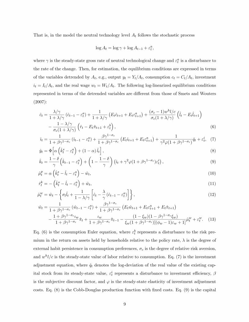
That is, in the model the neutral technology level At follows the stochastic process

logAt = log + logAt�1 + "at ;

where is the steady-state gross rate of neutral technological change and "at is a disturbance to

the rate of the change. Then, for estimation, the equilibrium conditions are expressed in terms

of the variables detrended by At, e.g., output yt = Yt=At, consumption ct = Ct=At, investment

it = It=At, and the real wage wt = Wt=At. The following log-linearized equilibrium conditions

represented in terms of the detrended variables are di¤erent from those of Smets and Wouters

(2007):

ct =�=

1 + �= (ct�1 � "at ) +

1

1 + �=

�Etct+1 + Et"

at+1

�+(�c � 1)whl=c�c(1 + �= )

�lt � Et lt+1

�� 1� �= �c(1 + �= )

�rt � Et�t+1 + "bt

�; (6)

{t =1

1 + � 1��c({t�1 � "at ) +

� 1��c

1 + � 1��c

�Et{t+1 + Et"

at+1

�+

1

2'(1 + � 1��c)qt + "

it; (7)

yt = �h��kst � "at

�+ (1� �) lt

i; (8)

kt =1� �

�kt�1 � "at

�+

�1� 1� �

��{t +

2'(1 + � 1��c)"it�; (9)

�pt = ��kst � lt � "at

�� wt; (10)

rkt = ��kst � lt � "at

�+ wt; (11)

�wt = wt ��l lt +

1

1� �=

�ct �

�

(ct�1 � "at )

��; (12)

wt =1

1 + � 1��c(wt�1 � "at ) +

� 1��c

1 + � 1��c

�Etwt+1 + Et"

at+1 + Et�t+1

�� 1 + �

1��c�w1 + � 1��c

�t +�w

1 + � 1��c�t�1 �

(1� �w)(1� � 1��c�w)�w(1 + � 1��c)[(�w � 1)"w + 1]

�wt + "wt : (13)

Eq. (6) is the consumption Euler equation, where "bt represents a disturbance to the risk pre-

mium in the return on assets held by households relative to the policy rate, � is the degree of

external habit persistence in consumption preferences, �c is the degree of relative risk aversion,

and whl=c is the steady-state value of labor relative to consumption. Eq. (7) is the investment

adjustment equation, where qt denotes the log-deviation of the real value of the existing cap-

ital stock from its steady-state value, "it represents a disturbance to investment e¢ ciency, �

is the subjective discount factor, and ' is the steady-state elasticity of investment adjustment

costs. Eq. (8) is the Cobb-Douglas production function with �xed costs. Eq. (9) is the capital

9

accumulation equation, where � is the depreciation rate of capital. Eq. (10) is the equation

for the price markup �pt , where wt is the real wage. Eq. (11) is the condition for capital and

labor inputs in production, where rkt is the real rental rate of capital. Eq. (12) is the equation

for the wage markup �wt , where �l is the inverse elasticity of labor supply. Eq. (13) is the

wage equation, where "wt represents a wage markup disturbance, �w and �w are the degrees

of wage stickiness and wage indexation to past in�ation, (�w � 1) is the steady-state labor

market markup, and "w is the curvature of the Kimball labor market aggregator. The other

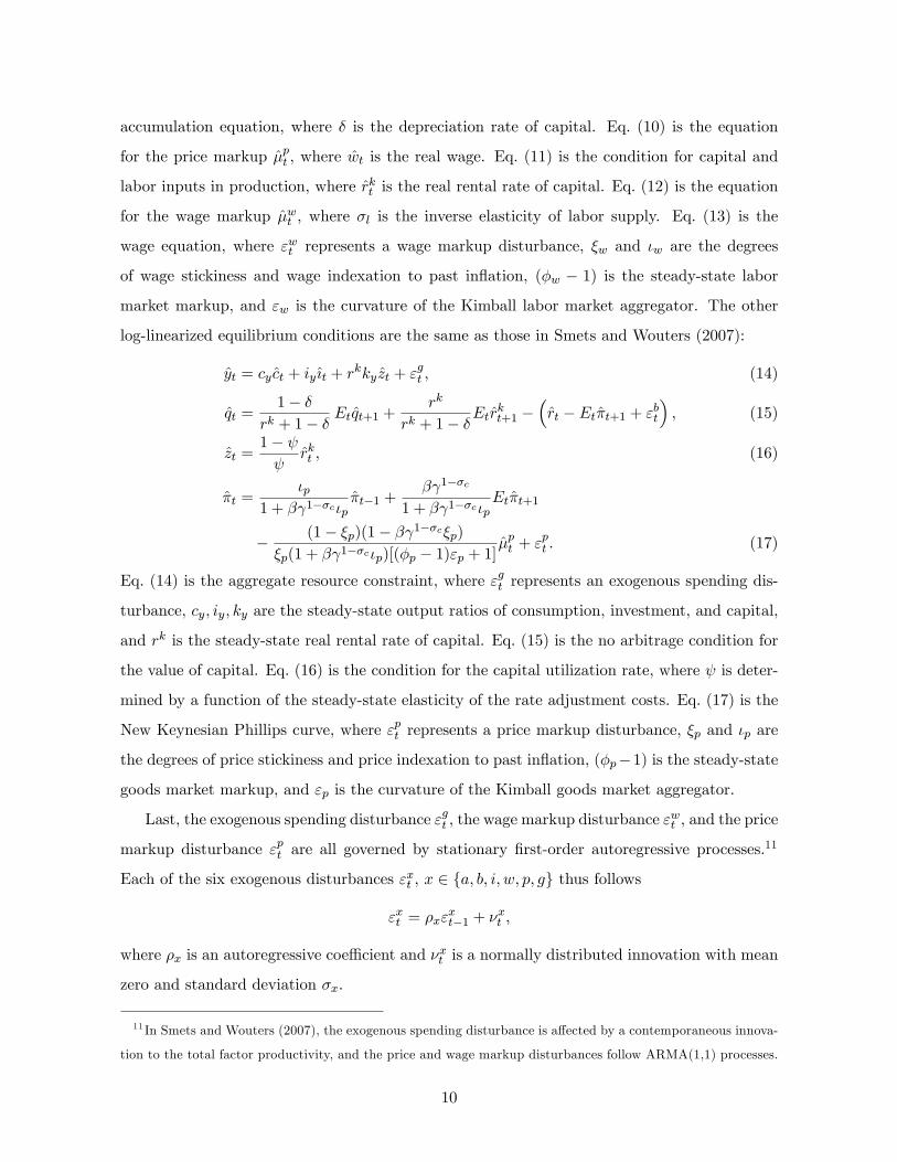
log-linearized equilibrium conditions are the same as those in Smets and Wouters (2007):

yt = cy ct + iy {t + rkky zt + "

gt ; (14)

qt =1� �

rk + 1� � Etqt+1 +rk

rk + 1� �Etrkt+1 �

�rt � Et�t+1 + "bt

�; (15)

zt =1�

rkt ; (16)

�t =�p

1 + � 1��c�p�t�1 +

� 1��c

1 + � 1��c�pEt�t+1

� (1� �p)(1� � 1��c�p)�p(1 + � 1��c�p)[(�p � 1)"p + 1]

�pt + "pt : (17)

Eq. (14) is the aggregate resource constraint, where "gt represents an exogenous spending dis-

turbance, cy; iy; ky are the steady-state output ratios of consumption, investment, and capital,

and rk is the steady-state real rental rate of capital. Eq. (15) is the no arbitrage condition for

the value of capital. Eq. (16) is the condition for the capital utilization rate, where is deter-

mined by a function of the steady-state elasticity of the rate adjustment costs. Eq. (17) is the

New Keynesian Phillips curve, where "pt represents a price markup disturbance, �p and �p are

the degrees of price stickiness and price indexation to past in�ation, (�p�1) is the steady-state

goods market markup, and "p is the curvature of the Kimball goods market aggregator.

Last, the exogenous spending disturbance "gt , the wage markup disturbance "wt , and the price

markup disturbance "pt are all governed by stationary �rst-order autoregressive processes.11

Each of the six exogenous disturbances "xt , x 2 fa; b; i; w; p; gg thus follows

"xt = �x"xt�1 + �

xt ;

where �x is an autoregressive coe¢ cient and �xt is a normally distributed innovation with mean

zero and standard deviation �x.

11 In Smets and Wouters (2007), the exogenous spending disturbance is a¤ected by a contemporaneous innova-

tion to the total factor productivity, and the price and wage markup disturbances follow ARMA(1,1) processes.

10

3.2 Econometric Methodology

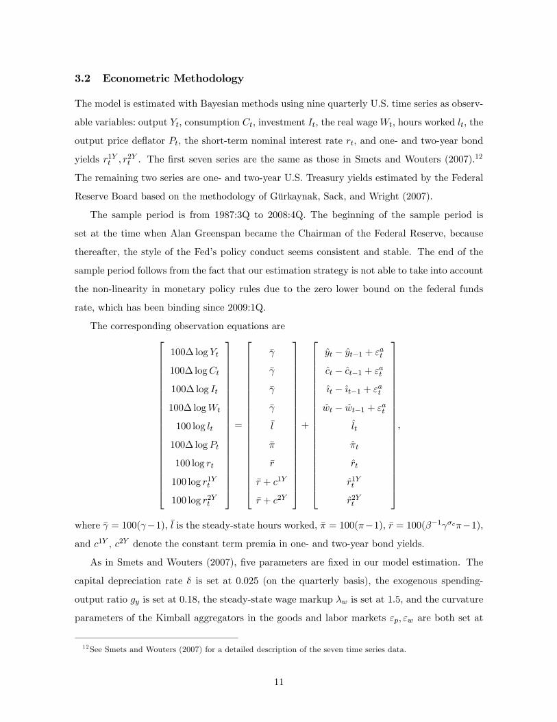
The model is estimated with Bayesian methods using nine quarterly U.S. time series as observ-

able variables: output Yt, consumption Ct, investment It, the real wageWt, hours worked lt, the

output price de�ator Pt, the short-term nominal interest rate rt, and one- and two-year bond

yields r1Yt ; r2Yt . The �rst seven series are the same as those in Smets and Wouters (2007).12

The remaining two series are one- and two-year U.S. Treasury yields estimated by the Federal

Reserve Board based on the methodology of Gürkaynak, Sack, and Wright (2007).

The sample period is from 1987:3Q to 2008:4Q. The beginning of the sample period is

set at the time when Alan Greenspan became the Chairman of the Federal Reserve, because

thereafter, the style of the Fed�s policy conduct seems consistent and stable. The end of the

sample period follows from the fact that our estimation strategy is not able to take into account

the non-linearity in monetary policy rules due to the zero lower bound on the federal funds

rate, which has been binding since 2009:1Q.

The corresponding observation equations are266666666666666666666664

100� log Yt

100� logCt

100� log It

100� logWt

100 log lt

100� logPt

100 log rt

100 log r1Yt

100 log r2Yt

377777777777777777777775

=

266666666666666666666664

�

�

�

�

�l

��

�r

�r + c1Y

�r + c2Y

377777777777777777777775

+

266666666666666666666664

yt � yt�1 + "atct � ct�1 + "at{t � {t�1 + "atwt � wt�1 + "at

lt

�t

rt

r1Yt

r2Yt

377777777777777777777775

;

where � = 100( �1), �l is the steady-state hours worked, �� = 100(��1), �r = 100(��1 �c��1),

and c1Y , c2Y denote the constant term premia in one- and two-year bond yields.

As in Smets and Wouters (2007), �ve parameters are �xed in our model estimation. The

capital depreciation rate � is set at 0.025 (on the quarterly basis), the exogenous spending-

output ratio gy is set at 0.18, the steady-state wage markup �w is set at 1.5, and the curvature

parameters of the Kimball aggregators in the goods and labor markets "p; "w are both set at

12See Smets and Wouters (2007) for a detailed description of the seven time series data.

11

10. For identi�cation, all innovations to the disturbances are, a priori, mutually and serially

uncorrelated.

The prior distributions of the parameters to be estimated are shown in the second to fourth

columns of Table 1. The same prior distributions as those in Smets and Wouters (2007) are

used. In addition, equal weights on the unanticipated component and on the total anticipated

component of monetary policy disturbances are used in the prior of these components�standard

deviations; that is, ��n, n = 1; 2; : : : ; 7 are distributed around 7�1=2 � 0:1 so thatP7n=1 �

2�n =

�2�0. The prior distributions of the constant term premia c1Y ; c2Y are set to be the normal

distributions with standard deviation 0.05 and mean given by the sample mean of the spreads

between the one- and two-year Treasury yields and the federal funds rate.

In the Bayesian estimation, the Kalman �lter is used to evaluate the likelihood function for

the system of log-linearized equilibrium conditions of the model, and the Metropolis-Hastings

algorithm is applied to generate draws from the posterior distribution of model parameters.13

Based on these draws, we make inference on the parameters and obtain the Kalman smoothed

estimates and the historical and variance decompositions of the model variables.

4 Empirical Results

This section presents the empirical results. First, the estimates of the model parameters are

shown. Then, the estimated series of monetary policy disturbances and their implications are

examined. Finally, several robustness exercises are conducted.

4.1 Parameter Estimates

Each parameter�s posterior mean and 90% posterior interval are reported in the last two

columns of Table 1. Basically, most of the estimates are similar to those in Table 5 of Smets

and Wouters (2007) for the sample period from 1984:1Q to 2004:4Q, since the model of the

present paper is a simple variant of their model. The estimated degrees of price stickiness and

policy rate smoothing (�p = 0:87, �R = 0:94) are higher than Smets and Wouters�estimates

(�p = 0:73, �R = 0:84). Moreover, the estimates of the autoregressive coe¢ cients of distur-

13 In each estimation, 500,000 draws are generated and the �rst half of these draws is discarded. The scale

factor for the jumping distribution in the Metropolis-Hastings algorithm is adjusted so that the acceptance rate

of 24% is obtained. The Brooks and Gelman measure is used to check the convergence of parameters.

12

bances to the neutral technology, the risk premium, and the wage markup (�a = 0:08, �b = 0:97,

�w = 0:25) di¤er from Smets and Wouters�estimates (�a = 0:94, �b = 0:14, �w = 0:74). These

di¤erences are attributed to the introduction of the stochastic trend in neutral technology as

well as the di¤erence in the sample period. For the same reason, the estimate of the standard

deviation of the innovation to neutral technological change (�a = 0:75) di¤ers from Smets and

Wouters�estimate (�a = 0:35).

The parameters speci�c to the present model are the constant term premia, c1Y ; c2Y ,

and the standard deviations of the anticipated components of monetary policy disturbances,

��1; ��2; : : : ; ��7. The estimates of c1Y = 0:04 and c2Y = 0:11 are almost the same as their

prior mean, each of which is set at the sample mean of the spread between the corresponding

bond yields and the federal funds rate. Although each of the estimates of ��1; ��2; : : : ; ��7 is

smaller than the estimate of ��0, the total variance of the anticipated components is larger than

the variance of the unanticipated component. This suggests the importance of the anticipated

components of monetary policy disturbances in the estimated model.

4.2 Historical Decomposition of Monetary Policy Disturbances

This subsection examines the changes in the Fed�s communication strategy during the 1990s

through a lens of the estimated series of the anticipated and unanticipated components of

monetary policy disturbances. The Fed decided in 1994 to release a statement describing

policy actions on the federal funds rate at the conclusion of any FOMC meeting at which a

policy action was undertaken,14 and determined in 1999 to issue a statement reporting the

settings of the target rate for the federal funds and the balance of risks to the Fed�s objectives

after every FOMC meeting. If these decisions on the Fed�s communication strategy are re�ected

in the U.S. bond yields, the e¤ects of the decisions should appear in the estimated series of the

anticipated and unanticipated components of the policy disturbances.

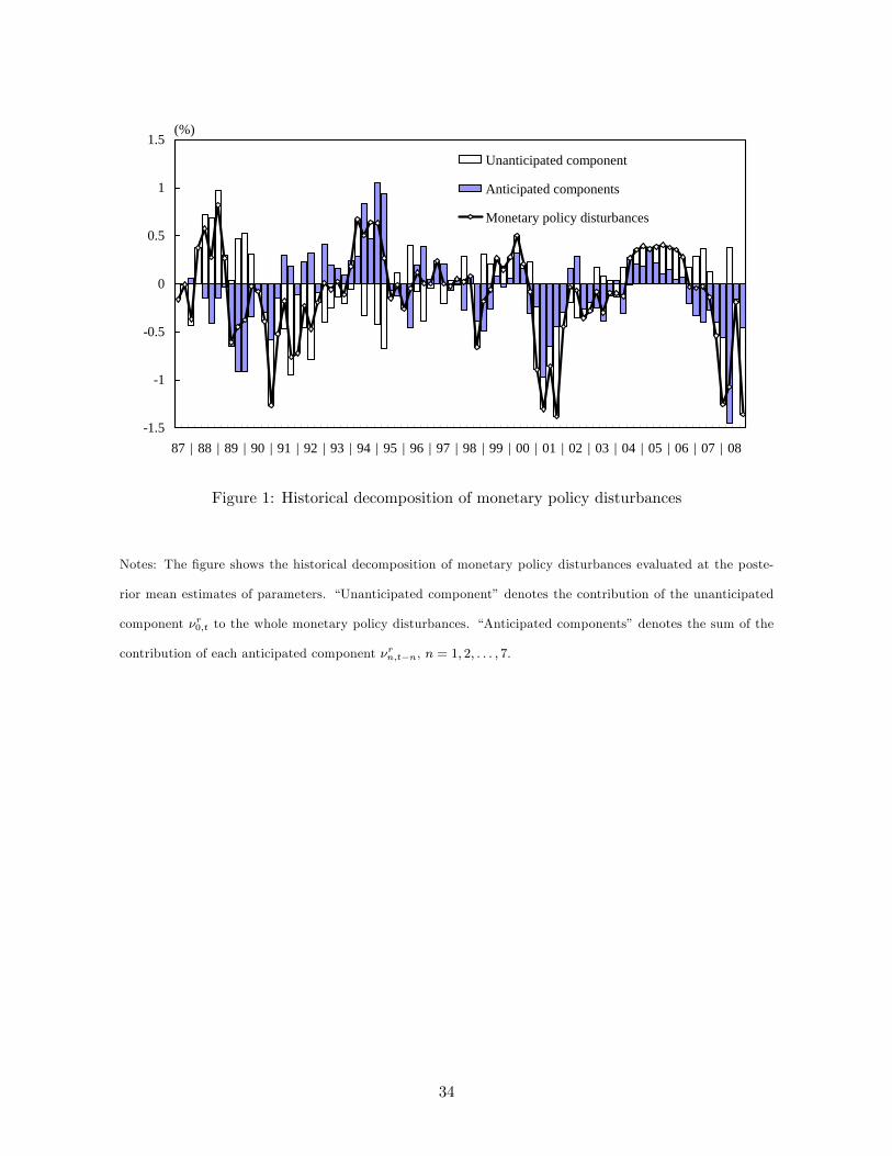
Figure 1 illustrates the historical decomposition of monetary policy disturbances into the

unanticipated and the total anticipated components, evaluated at the posterior mean estimates

of parameters. The estimated series of the policy disturbances consist mainly of the anticipated

component during the sample period, i.e., the Greenspan-Bernanke era. From a historical

14Goodfriend (2010) mentions that this decision �was a dramatic moment for those in the room like the author

who were aware of the longstanding reluctance of the Fed to be fully clear about its interest rate policy, and for

those who thought more openness was necessary and bene�cial�(p. 3).

13

perspective, the relationship between the unanticipated and the total anticipated components

changed after the mid-1990s. The total anticipated component was o¤set by the unanticipated

one until the mid-1990s, but thereafter, both the components contributed to the whole policy

disturbances in almost the same direction.15 That is, a large fraction of the total anticipated

component was not met before the mid-1990s, but thereafter, the total anticipated component

tended to materialize.

4.3 Subsample Analysis

The historical decomposition of monetary policy disturbances has shown that the relationship

between the unanticipated and the anticipated components changed after the mid-1990s. To

investigate this change in more detail, the model is estimated for two subsamples: 1987:3Q�

1996:4Q and 1997:1Q�2008:4Q. Each parameter�s posterior mean and 90% posterior interval

in the two subsamples are reported in Table 2. Most of the parameter estimates are similar

between these two subsamples, but there is a remarkable di¤erence in the estimate of the

standard deviation of the unanticipated component of monetary policy disturbances. The

variance of the unanticipated component became smaller in the latter subsample (��0 = 0:12

for 1987:3Q�1996:4Q, ��0 = 0:07 for 1997:1Q�2008:4Q).16 This result implies that after the

mid-1990s, the relative importance of the unanticipated component was diminished and the

Fed focused more on the role of the anticipated component in its policy conduct. This �nding

is also con�rmed by the variance decomposition of monetary policy disturbances presented

in Table 3. This table indicates the relative importance of the unanticipated and the total

anticipated components in the whole policy disturbances, and shows that the contribution of

the total anticipated component relative to the unanticipated one became much larger in the

latter subsample (59.0% for 1987:3Q�1996:4Q, 80.5% for 1997:1Q�2008:4Q).

The above historical decomposition and subsample analysis of monetary policy disturbances

demonstrate that until the mid-1990s, the Fed made its future policy actions unanticipated for

15 In the econometric approach, all components of monetary policy disturbances are, a priori, mutually uncor-

related. However, they can be, ex post, correlated with each other as shown in this result.

16There are also di¤erences in the standard deviation of the innovation to neutral technological changes, the

autoregressive coe¢ cient of the wage markup disturbance, and the standard deviation of the innovation to the

markup disturbance (�a = 0:55; �w = 0:82; �w = 0:10 for 1987:3Q�1996:4Q; �a = 0:87; �w = 0:21; �w = 0:37 for

1997:1Q�2008:4Q).

14

participants in �nancial markets. Indeed, Greenspan (1989) stated in the Congress that �a

public announcement requirement also could impede timely and appropriate adjustments to

policy.�17 After the mid-1990s, the Fed tended to coordinate �nancial market expectations

about future policy actions, i.e., the future path of the federal funds rate. According to Good-

friend (2010), the Fed, in the mid-1990s, was inclined to talk openly in terms of interest rate

policy, since academics had begun to do so a few years earlier and an academic literature

had developed indicating that communication could enhance the e¤ectiveness of the policy.18

In this context, Woodford (2001, 2003, 2005) insists that central banks�ability to a¤ect the

economy depends crucially on their ability to manage �nancial market expectations about the

future path of the policy rate. Particularly, Woodford stresses that better information on the

part of market participants about the central banks�actions and intensions increases the degree

to which the banks�policy decisions can actually in�uence the market expectations on future

policy actions, and thereby improves the e¤ectiveness of monetary policy. These arguments

suggest that the changes in the Fed�s communication strategy are consistent with the rise in

the academic views on central banking as management of expectations. For this management,

Blinder et al. (2008) emphasize the role of �news�or �signals�by central banks. The antici-

pated monetary policy disturbances examined in the present paper can be regarded as a form

of such news or signals by the Fed. Therefore, the �nding about the importance of the an-

ticipated policy disturbances after the mid-1990s would re�ect the Fed�s understanding of the

importance of managing expectations about its future policy actions (i.e., forward guidance on

the policy rate).

The �nding regarding the composition of the anticipated and unanticipated components of

monetary policy disturbances poses the questions of whether and how the business cycle im-

plications of the policy disturbances changed after the mid-1990s. Table 4 reports the variance

17Goodfriend (1986) documented the Fed�s defense of secrecy and argued against central bank secrecy.

18Goodfriend (2010) also raises three practical reasons for the change in the Fed�s communication strategy in

1994. First, more timely announcements of policy actions would not impair the FOMC�s deliberative process,

which it was most anxious to protect. Second, to do otherwise would be to invite leaks of its intended policy

stance. Third, continued delayed announcement of its interest rate policy stance would feed into an increasingly

unfavorable opinion about the Fed�s secrecy building in Congress and the media. Indeed, in the FOMC meeting

held in November 1993, Greenspan�s concern was to avoid �premature, detailed disclosure of our deliberations�

that would compromise the �openness and free exchange of views so essential to monetary policy�(FOMC

Transcripts, November 16, 1993, p. 6).

15

decompositions of output growth, consumption growth, investment growth, and hours worked

in each subsample.19 The relative contribution of the total anticipated component of the pol-

icy disturbances to the variances of the four macroeconomic variables increased in the latter

subsample, whereas the contribution of the unanticipated component declined. This suggests

that after the mid-1990s, the expectation channel by the anticipated components of monetary

policy disturbances played a larger role in the transmission mechanism of the Fed�s monetary

policy to the U.S. economy.

4.4 Importance of Bond Yields Data in Estimation

Thus far, the paper has identi�ed the anticipated and unanticipated components of monetary

policy disturbances by including bond yields in the data for model estimation. However, as in

Milani and Treadwell (2009), it may be possible to identify these components without using

the bond yields data because the anticipated component has a di¤erent e¤ect on output than

the unanticipated one.20 Thus, in order to examine the importance of bond yields data in

our estimation, this subsection estimates the model without using the bond yields data and

compares the result with that of the baseline estimation.

The second and third columns of Table 5 report the posterior mean and the 90% posterior

interval of each parameter in the model estimated with no bond yields data.21 Although most of

these estimates are similar to the baseline estimates presented in the last two columns of Table 1,

there are crucial di¤erences in the estimates of the standard deviations of the unanticipated

component and the two-period-ahead anticipated component of monetary policy disturbances.22

In the absence of bond yields data, the estimated variances of the anticipated and unanticipated

components are smaller (��0 = 0:10; ��2 = 0:08 in the baseline estimation, ��0 = 0:05; ��2 =

19Table 4 presents the decompositions of the asymptotic forecast error variances at an in�nite horizon. Almost

the same result is obtained even when the variance decompositions are computed at the business cycle frequency,

e.g., 8 and 32 quarters. These variance decompositions are available upon request. The same argument applies

to Tables 6 and 8.

20Milani and Treadwell (2009) indicate that the anticipated component of monetary policy disturbances has

a larger, more delayed, and more persistent e¤ect on output than the unanticipated one.

21The prior distributions are the same as those in the baseline estimation shown in the second to fourth

columns of Table 1.

22There is also a di¤erence in the degree of policy rate smoothing (�R = 0:94 in the baseline estimation, �R =

0:67 in the estimation with no bond yields data).

16

0:03 in the estimation with no bond yields data).

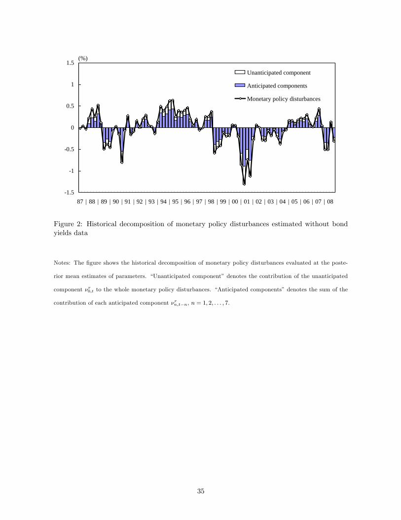
To see how these di¤erences a¤ect the estimated series of the unanticipated and the total

anticipated components of monetary policy disturbances, Figure 2 illustrates the historical

decomposition of the disturbances, evaluated at the posterior mean estimates without using

the bond yields data. The decomposition in this �gure is radically di¤erent from the one

based on the baseline estimates in Figure 1. The former shows that throughout the sample

period, both the unanticipated and the total anticipated components contributed in the same

direction to the whole monetary policy disturbances, suggesting no qualitative change in the

policy disturbances. Therefore, in the absence of the bond yields data in model estimation, the

estimated series of monetary policy disturbances is not able to capture the actual changes in

the Fed�s communication strategy during the 1990s.

These changes in the estimates can also alter the e¤ect of monetary policy disturbances on

macroeconomic volatilities. Table 6 compares the variance decompositions of output growth,

consumption growth, investment growth, and hours worked between the baseline estimates

shown in the �rst four rows and the estimates with no bond yields data in the �fth to eighth

rows. This comparison shows that the magnitude of the contribution of monetary policy dis-

turbances relative to the other disturbances is dramatically di¤erent. While the contribution

of the whole monetary policy disturbances is around 15%�30% in the baseline estimation, it is

around 0.5%�1% in the estimation with no bond yields data. Therefore, the use of the bond

yields data in model estimation leads to a substantial relative contribution of the monetary

policy disturbances to business cycles.

For comparison, the model with no anticipated component of monetary policy disturbances

is estimated.23 The fourth and �fth columns of Table 5 report the posterior mean and the 90%

posterior interval of each parameter. All of the estimates, except the standard deviation of the

unanticipated component, are almost the same as those with no bond yields data presented in

the second and third columns of the same table. The estimated variance of the unanticipated

monetary policy disturbances is larger in the absence of the anticipated components (��0 = 0:1

in the model with no anticipated components, ��0 = 0:05 in the baseline model estimated with

no bond yields data). The last four rows of Table 6 show the variance decompositions of output

23Note that no bond yields data is used for this estimation. The estimation of the model with no anticipated

component of monetary policy disturbances using bond yields data leads to the singularity of the likelihood

function, since the number of data series exceeds the number of disturbances in the model.

17

growth, consumption growth, investment growth, and hours worked in the estimated model

with no anticipated component of monetary policy disturbances. This decomposition indicates

that the relative contribution of monetary policy disturbances is quite marginal, as is the case

with the baseline model estimated with no bond yields data. Therefore, the exclusion of the

bond yields data in model estimation makes the contribution of monetary policy disturbances

to business cycles negligible, regardless of whether or not the anticipated components of the

policy disturbances are incorporated.

4.5 Robustness Analysis

This subsection assesses the robustness of the baseline results in the following three respects.

First, an alternative speci�cation of the monetary policy rule is examined. Second, time-varying

components of term premia are allowed in one- and two-year bond yields. Third, the data on

bond yields excluding term premia are used in model estimation. These three robustness

exercises are conducted in turn.

4.5.1 Alternative Speci�cation of Monetary Policy Rule

The misspeci�cation of the monetary policy rule directly a¤ects the estimates of its distur-

bances, and hence may change the qualitative properties of the baseline results. Thus, an

alternative speci�cation of the policy rule is estimated together with the rest of the baseline

model. The speci�cation examined here adds the policy response to the deviation of the output

growth rate from its steady-state value (i.e., 100� log Yt � � = yt � yt�1 + "at ) to the baseline

speci�cation.

rt = �Rrt�1 + (1� �R)"r�

1

4

3Xn=0

�t�n

!+ ry(yt � y�t )

#+ r�y (yt � yt�1 + "at ) + "rt ;

where r�y is the degree of the policy response to output growth. This speci�cation expresses the

Fed�s concern about stable growth of the U.S. economy in its policy conduct. The speci�cation

is very close to the one used by Smets and Wouters (2007), in which the policy rate is adjusted

in response to the change in the (theoretical) output gap.24 The prior of r�y is thus set to

be the normal distribution with mean 0.125 and standard deviation 0.05, following Smets and

Wouters (2007).

24Adding the policy response to the change in our practical output gap has been also investigated. We have

con�rmed that the results are almost the same.

18

In Table 7, the second and third columns report the posterior mean and the 90% posterior

interval of each parameter in the estimated model with the alternative speci�cation of the mon-

etary policy rule. The estimated degree of the policy response to output growth (r�y = 0:09)

is smaller than its prior mean, and the estimates of the other parameters are not remarkably

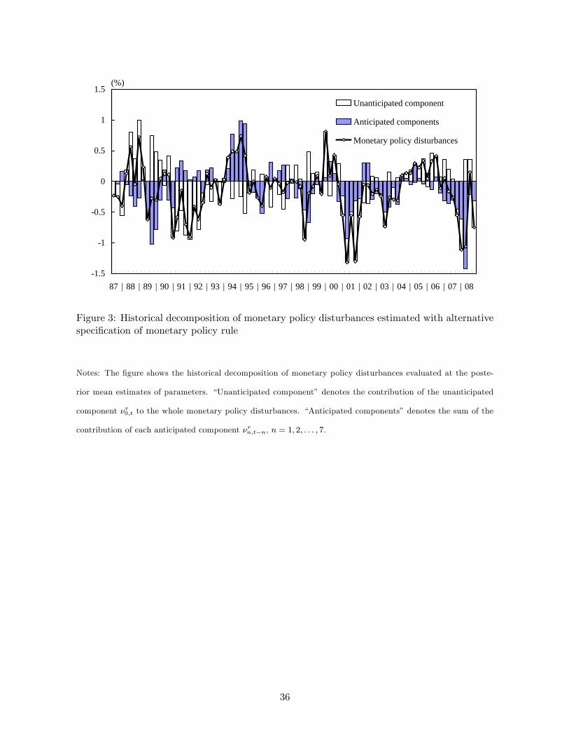
di¤erent from those in the case of the baseline speci�cation shown in Table 1. Figure 3 il-

lustrates the historical decomposition of monetary policy disturbances. This decomposition is

very similar to that in the baseline shown in Figure 1. The �fth to eighth rows of Table 8

show the variance decompositions of output growth, consumption growth, investment growth,

and hours worked under the alternative policy rule. The monetary policy disturbances, their

total anticipated component in particular, have a substantial contribution to the �uctuations

in the four macroeconomic variables, as is the case with the baseline policy rule presented in

the �rst four rows of the same table. Therefore, the baseline results are robust with respect to

the alternative speci�cation of the monetary policy rule.

4.5.2 Time-Varying Term Premia

The second robustness exercise allows for time-varying components of term premia in one-

and two-year bond yields. In these relatively short-term bond yields, the baseline model has

assumed the constant term premia, and as a consequence, the estimates of the anticipated mon-

etary policy disturbances may contain the possible time-varying components of term premia.

To investigate this issue, the present exercise follows De Graeve, Emiris, and Wouters (2009)

to replace the observation equations for one- and two-year bond yields by24 100 log r1Yt100 log r2Yt

35 =24 �r + c1Y

�r + c2Y

35+24 r1Yt + �1Yt

r2Yt + �2Yt

35;where �1Yt ; �2Yt represent the measurement errors interpreted as the time-varying components of

term premia in one- and two-year bond yields and evolve according to the stochastic processes

�1Yt = �1Y �1Yt�1 + �

1Yt ;

�2Yt = �2Y �2Yt�1 + �

2Yt ;

where �1Y ; �2Y are autoregressive coe¢ cients and �1Yt ; �2Yt are normally distributed innovations

with mean zero and standard deviation �1Y ; �2Y , respectively. The prior distributions of the

autoregressive coe¢ cients �1Y ; �2Y and the standard deviations �1Y ; �2Y are the same as those

19

for the other disturbances, i.e., the beta distributions with mean 0.5 and standard deviation

0.2 for �1Y ; �2Y and the inverse gamma distributions with mean 0.1 and standard deviation 2

for �1Y ; �2Y .

The fourth and �fth columns of Table 7 report each parameter�s posterior mean and 90%

posterior interval in the presence of the time-varying components of term premia. The estimated

standard deviations of the innovations to term premia (�1Y = 0:02; �2Y = 0:03) are comparable

to that of each anticipated monetary policy disturbance, and the estimated degrees of the

persistence of term premia (�1Y = 0:78; �2Y = 0:84) are larger than their prior mean. The

other estimates are almost the same as the baseline estimates presented in Table 1. Even when

the time-varying components of term premia are introduced in the bond yields, the historical

decomposition of monetary policy disturbances illustrated in Figure 4 is very similar to that for

the baseline model in Figure 1. Table 8 compares the variance decompositions of output growth,

consumption growth, investment growth, and hours worked between the baseline estimates

shown in the �rst four rows and the estimates with the time-varying term premia in the ninth to

twelfth rows. Although the contribution of anticipated monetary policy disturbances is smaller

in the estimates with the time-varying term premia, it remains su¢ ciently large. Therefore,

the baseline results still hold even when the model allows for the time-varying components of

term premia in the bond yields.

4.5.3 Alternative Data on Bond Yields

The last robustness exercise concerns another way to resolve the issue regarding the inclusion

of possible time-varying components of the bond yields�term premia in anticipated monetary

policy disturbances. The exercise conducted here is the use of the data on bond yields excluding

term premia in model estimation. Speci�cally, the observation equations for one- and two-year

bond yields are replaced by 24 100 log ~r1Yt100 log ~r2Yt

35 =24 �r

�r

35+24 r1Yt

r2Yt

35;where ~r1Yt ; ~r2Yt represent the gross rates of one- and two-year bond yields excluding term premia,

estimated by the Federal Reserve Board based on the methodology of Kim and Wright (2005).

The posterior mean and the 90% posterior interval of each parameter in the baseline model

estimated with the data on bond yields excluding term premia are reported in the last two

20

columns of Table 7. The estimates are very similar to those in the baseline. According to the

historical decomposition of monetary policy disturbances illustrated in Figure 5, the alternative

bond yields data leads to the somewhat obvious compositional change in monetary policy

disturbances. The total anticipated component of the policy disturbances was o¤set by the

unanticipated one in the 1990s, and thereafter, both the components tended to contribute

in almost the same direction. Regarding the importance of monetary policy disturbances in

business cycles, the last four rows of Table 8 show that the relative contribution of each policy

disturbance is slightly smaller than that in the baseline estimation but larger than that in

the model with time-varying term premia in the bond yields. These demonstrate that the

qualitative properties of the baseline results still hold even with the use of the alternative bond

yields data in the estimation.

5 Concluding Remarks

This paper has structurally investigated the changes in the Fed�s communication strategy during

the 1990s through a lens of the anticipated and unanticipated components of monetary policy

disturbances. These components have been identi�ed in a version of Smets and Wouters�(2007)

model with the term structure of interest rates, using the U.S. data that includes bond yields.

According to the estimation results, the Fed made its future policy actions unanticipated for

�nancial market participants until the mid-1990s, but thereafter, the Fed placed more emphasis

on the coordination of the market expectations about the future policy actions, re�ecting the

rise of the academic views on central banking as management of expectations. It is important

to stress that the inclusion of bond yields in the data for estimation is indispensable to the

meaningful change in the composition of the anticipated and unanticipated components of

monetary policy disturbances in the mid-1990s. This is because the bond yields contain crucial

information on the expected future path of the federal funds rate. Moreover, it has been

demonstrated that the model estimated with the bond yields data suggests substantial in�uence

of monetary policy disturbances on business cycles whereas the model without them does not.

A more detailed investigation of the estimated series of the anticipated component of mon-

etary policy disturbances would help to understand the Fed�s forward guidance on the federal

funds rate. For instance, the estimation results suggest that in 2003 and 2008, the Fed success-

fully coordinated �nancial market expectations so that the market participants could anticipate

21

that the federal funds rate would be lower than that suggested by the estimated Taylor rule

for some time in the future. Then, the questions arise as to how and to what extent this man-

agement of expectations by the Fed in�uenced the U.S. macroeconomic performance in those

periods. Addressing these issues is left for future research.

22

References

[1] Beaudry, Paul, and Franck Portier. 2004. �An Exploration into Pigou�s Theory of Cycles.�

Journal of Monetary Economics, 51(6), 1183�1216.

[2] Bernanke, Ben S. 2003. ��Constrained Discretion�and Monetary Policy.�Remarks before

the Money Marketeers of New York University, New York, February 3.

[3] Blinder, Alan S., Charles Goodhart, Philipp Hildebrand, David Lipton, and Charles

Wyplosz. 2001. How Do Central Banks Talk? Geneva Report on the World Economy

No. 3, International Center for Monetary and Banking Studies.

[4] Blinder, Alan S., Michael Ehrmann, Marcel Fratzscher, Jakob De Haan, and David-Jan

Jansen. 2008. �Central Bank Communication and Monetary Policy: A Survey of Theory

and Evidence.�Journal of Economic Literature, 46(4), 910�945.

[5] Christiano, Lawrence, Cosmin L. Ilut, Roberto Motto, and Massimo Rostagno. 2010.

�Monetary Policy and Stock Market Booms.�NBER Working Paper Series, No. 16402,

National Bureau of Economic Research.

[6] Clarida, Richard, Jordi Galí, and Mark Gertler. 1998. �Monetary Policy Rules in Practice:

Some International Evidence.�European Economic Review, 42(6), 1033�1067.

[7] Clarida, Richard, Jordi Galí, and Mark Gertler. 2000. �Monetary Policy Rules and Macro-

economic Stability: Evidence and Some Theory.�Quarterly Journal of Economics, 115(1),

147�180.

[8] De Graeve, Ferre, Marina Emiris, and Raf Wouters. 2009. �A Structural Decomposition

of the US yield curve.�Journal of Monetary Economics, 56(4), 545�559.

[9] Fujiwara, Ippei. 2010. �A Note on Growth Expectation.�Macroeconomic Dynamics, 14(2),

242�256.

[10] Fujiwara, Ippei, Yasuo Hirose, and Mototsugu Shintani. 2011. �Can News Be a Major

Source of Aggregate Fluctuations? A Bayesian DSGE Approach.� Journal of Money,

Credit and Banking, 43(1), 1�29.

23

[11] Goodfriend, Marvin. 1986. �Monetary Mystique: Secrecy and Central Banking.�Journal

of Monetary Economics, 17(1), 63�92.

[12] Goodfriend, Marvin. 1991. �Interest Rates and the Conduct of Monetary Policy�Carnegie

Rochester Conference Series on Public Policy, 34(1), 7�30.

[13] Goodfriend, Marvin. 2010. �Policy Debates at the FOMC: 1993�2002.�Prepared for the

Federal Reserve Bank of Atlanta-Rutgers University Conference, A Return to Jekyll Is-

land: The Origins, History, and Future of the Federal Reserve, November 5�6.

[14] Greenspan, Alan. 1989. Testimony before the Subcommittee on Domestic Monetary Policy

of the Committee on Banking, Finance and Urban A¤airs, U.S. House of Representatives,

Washington, D.C., October 25.

[15] Gürkaynak, Refet S., Brian Sack, and Jonathan H. Wright. 2007. �The U.S. Treasury Yield

Curve: 1961 to the Present.�Journal of Monetary Economics, 54(8), 2291�2304.

[16] Jaimovich, Nir, and Sergio Rebelo. 2009. �Can News about the Future Drive the Business

Cycle?�American Economic Review, 99(4), 1097�1118.

[17] Judd, John F., and Glenn D. Rudebusch. 1998. �Taylor�s Rule and the Fed: 1970�1997.�

Federal Reserve Bank of San Francisco Economic Review, 1998(3), 3�16.

[18] Khan, Hashmat, and John Tsoukalas. 2009. �The Quantitative Importance of News Shocks

in Estimated DSGE Models.�Carleton Economic Papers 09-07, Carleton University.

[19] Kim, Don H., and Jonathan H. Wright. 2005. �An Arbitrage-Free Three-Factor Term

Structure Model and the Recent Behavior of Long-Term Yields and Distant-Horizon For-

ward Rates.�Finance and Economics Discussion Series, No. 2005-33, Board of Governors

of the Federal Reserve System.

[20] Lorenzoni, Guido. 2009. �A Theory of Demand Shocks.� American Economic Review,

99(5), 2050�2084.

[21] Milani, Fabio, and John Treadwell. 2009. �The E¤ects of Monetary Policy �News� and

�Surprises�.�Mimeo, University of California, Irvine.

[22] Orphanides, Athanasios. 2001. �Monetary Policy Rules Based on Real-Time Data.�Amer-

ican Economic Review, 91(4), 964�985.

24

[23] Orphanides, Athanasios. 2002. �Monetary-Policy Rules and the Great In�ation.�American

Economic Review, 92(2), 115�120.

[24] Orphanides, Athanasios. 2003. �Historical Monetary Policy Analysis and the Taylor Rule.�

Journal of Monetary Economics, 50(5), 983�1022.

[25] Schmitt-Grohe, Stephanie, and Martin Uribe. 2008. �What�s News in Business Cycles?�

NBER Working Paper Series, No. 14215, National Bureau of Economic Research.

[26] Smets, Frank, and Rafael Wouters. 2007. �Shocks and Frictions in US Business Cycles: A

Bayesian DSGE Approach.�American Economic Review, 97(3), 586�606.

[27] Taylor, John B. 1993. �Discretion Versus Policy Rules in Practice.�Carnegie-Rochester

Conference Series on Public Policy, 39(1), 195�214.

[28] Taylor, John B. 1999. �A Historical Analysis of Monetary Policy Rules.�In John B. Taylor

(ed.), Monetary Policy Rules, University of Chicago Press, Chicago, 319�341.

[29] Woodford, Michael. 2001. �Monetary Policy in the Information Economy.� In Economic

Policy for the Information Economy, Federal Reserve Bank of Kansas City, Kansas City,

297�370.

[30] Woodford, Michael. 2003. Interest and Prices: Foundations of a Theory of Monetary Pol-

icy, Princeton University Press, Princeton.

[31] Woodford, Michael. 2005. �Central-Bank Communication and Policy E¤ectiveness.� In

The Greenspan Era: Lessons for the Future, Federal Reserve Bank of Kansas City, Kansas

City, 399�474.

[32] Woodford, Michael. 2008. �The Fed�s New Communication Strategy: Is It Stealth In�ation

Targeting?�Business Economics, 43(3), 7�13.

25

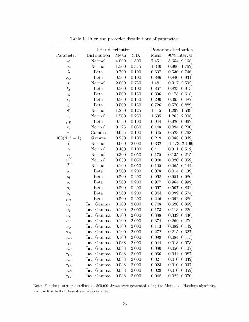
Table 1: Prior and posterior distributions of parameters

Prior distribution Posterior distributionParameter Distribution Mean S.D. Mean 90% interval

' Normal 4.000 1.500 7.451 [5.654, 9.168]�c Normal 1.500 0.375 1.340 [0.906, 1.762]� Beta 0.700 0.100 0.637 [0.530, 0.746]�w Beta 0.500 0.100 0.886 [0.840, 0.931]�l Normal 2.000 0.750 1.481 [0.317, 2.592]�p Beta 0.500 0.100 0.867 [0.823, 0.913]�w Beta 0.500 0.150 0.396 [0.175, 0.618]�p Beta 0.500 0.150 0.290 [0.095, 0.487] Beta 0.500 0.150 0.726 [0.570, 0.889]� Normal 1.250 0.125 1.415 [1.292, 1.539]r� Normal 1.500 0.250 1.635 [1.263, 2.008]�R Beta 0.750 0.100 0.944 [0.926, 0.962]ry Normal 0.125 0.050 0.148 [0.094, 0.200]�� Gamma 0.625 0.100 0.645 [0.523, 0.768]

100(��1 � 1) Gamma 0.250 0.100 0.219 [0.088, 0.349]�l Normal 0.000 2.000 0.332 [-1.473, 2.109]� Normal 0.400 0.100 0.411 [0.311, 0.512]� Normal 0.300 0.050 0.175 [0.135, 0.215]c1Y Normal 0.030 0.050 0.040 [0.020, 0.059]c2Y Normal 0.100 0.050 0.105 [0.065, 0.144]�a Beta 0.500 0.200 0.078 [0.014, 0.139]�b Beta 0.500 0.200 0.968 [0.951, 0.986]�g Beta 0.500 0.200 0.977 [0.964, 0.992]�I Beta 0.500 0.200 0.667 [0.507, 0.832]�p Beta 0.500 0.200 0.344 [0.099, 0.574]�w Beta 0.500 0.200 0.246 [0.092, 0.389]�a Inv. Gamma 0.100 2.000 0.748 [0.626, 0.869]�b Inv. Gamma 0.100 2.000 0.173 [0.113, 0.229]�g Inv. Gamma 0.100 2.000 0.388 [0.339, 0.436]�I Inv. Gamma 0.100 2.000 0.374 [0.269, 0.479]�p Inv. Gamma 0.100 2.000 0.113 [0.082, 0.142]�w Inv. Gamma 0.100 2.000 0.272 [0.215, 0.327]��0 Inv. Gamma 0.100 2.000 0.099 [0.084, 0.113]��1 Inv. Gamma 0.038 2.000 0.044 [0.013, 0.073]��2 Inv. Gamma 0.038 2.000 0.080 [0.056, 0.107]��3 Inv. Gamma 0.038 2.000 0.066 [0.044, 0.087]��4 Inv. Gamma 0.038 2.000 0.021 [0.010, 0.032]��5 Inv. Gamma 0.038 2.000 0.023 [0.010, 0.037]��6 Inv. Gamma 0.038 2.000 0.029 [0.010, 0.052]��7 Inv. Gamma 0.038 2.000 0.048 [0.022, 0.070]

Note: For the posterior distribution, 500,000 draws were generated using the Metropolis-Hastings algorithm,

and the �rst half of these draws was discarded.

26

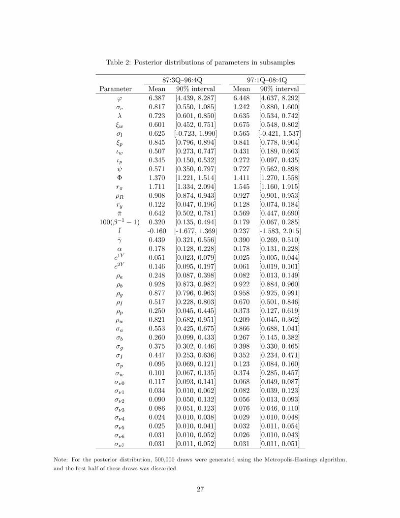
Table 2: Posterior distributions of parameters in subsamples

87:3Q�96:4Q 97:1Q�08:4QParameter Mean 90% interval Mean 90% interval

' 6.387 [4.439, 8.287] 6.448 [4.637, 8.292]�c 0.817 [0.550, 1.085] 1.242 [0.880, 1.600]� 0.723 [0.601, 0.850] 0.635 [0.534, 0.742]�w 0.601 [0.452, 0.751] 0.675 [0.548, 0.802]�l 0.625 [-0.723, 1.990] 0.565 [-0.421, 1.537]�p 0.845 [0.796, 0.894] 0.841 [0.778, 0.904]�w 0.507 [0.273, 0.747] 0.431 [0.189, 0.663]�p 0.345 [0.150, 0.532] 0.272 [0.097, 0.435] 0.571 [0.350, 0.797] 0.727 [0.562, 0.898]� 1.370 [1.221, 1.514] 1.411 [1.270, 1.558]r� 1.711 [1.334, 2.094] 1.545 [1.160, 1.915]�R 0.908 [0.874, 0.943] 0.927 [0.901, 0.953]ry 0.122 [0.047, 0.196] 0.128 [0.074, 0.184]�� 0.642 [0.502, 0.781] 0.569 [0.447, 0.690]

100(��1 � 1) 0.320 [0.135, 0.494] 0.179 [0.067, 0.285]�l -0.160 [-1.677, 1.369] 0.237 [-1.583, 2.015]� 0.439 [0.321, 0.556] 0.390 [0.269, 0.510]� 0.178 [0.128, 0.228] 0.178 [0.131, 0.228]c1Y 0.051 [0.023, 0.079] 0.025 [0.005, 0.044]c2Y 0.146 [0.095, 0.197] 0.061 [0.019, 0.101]�a 0.248 [0.087, 0.398] 0.082 [0.013, 0.149]�b 0.928 [0.873, 0.982] 0.922 [0.884, 0.960]�g 0.877 [0.796, 0.963] 0.958 [0.925, 0.991]�I 0.517 [0.228, 0.803] 0.670 [0.501, 0.846]�p 0.250 [0.045, 0.445] 0.373 [0.127, 0.619]�w 0.821 [0.682, 0.951] 0.209 [0.045, 0.362]�a 0.553 [0.425, 0.675] 0.866 [0.688, 1.041]�b 0.260 [0.099, 0.433] 0.267 [0.145, 0.382]�g 0.375 [0.302, 0.446] 0.398 [0.330, 0.465]�I 0.447 [0.253, 0.636] 0.352 [0.234, 0.471]�p 0.095 [0.069, 0.121] 0.123 [0.084, 0.160]�w 0.101 [0.067, 0.135] 0.374 [0.285, 0.457]��0 0.117 [0.093, 0.141] 0.068 [0.049, 0.087]��1 0.034 [0.010, 0.062] 0.082 [0.039, 0.123]��2 0.090 [0.050, 0.132] 0.056 [0.013, 0.093]��3 0.086 [0.051, 0.123] 0.076 [0.046, 0.110]��4 0.024 [0.010, 0.038] 0.029 [0.010, 0.048]��5 0.025 [0.010, 0.041] 0.032 [0.011, 0.054]��6 0.031 [0.010, 0.052] 0.026 [0.010, 0.043]��7 0.031 [0.011, 0.052] 0.031 [0.011, 0.051]



27

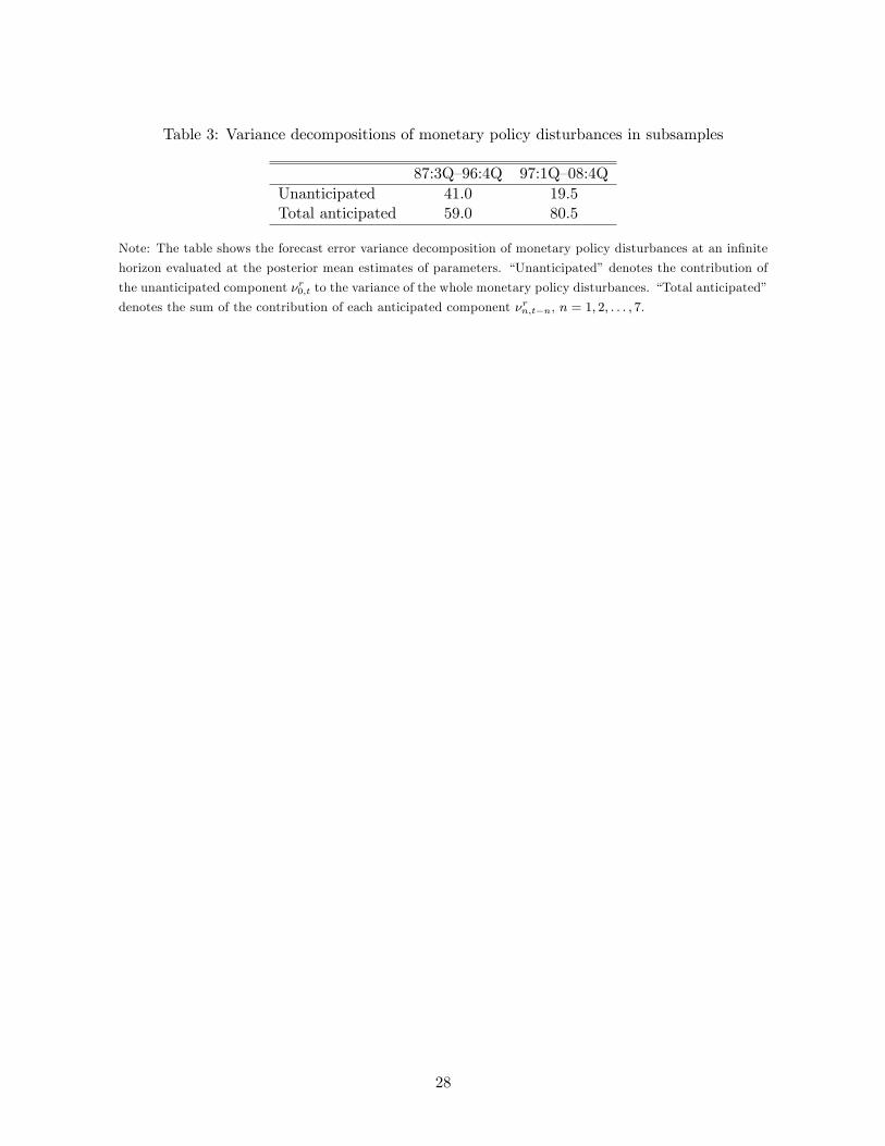
Table 3: Variance decompositions of monetary policy disturbances in subsamples

87:3Q�96:4Q 97:1Q�08:4QUnanticipated 41.0 19.5Total anticipated 59.0 80.5

Note: The table shows the forecast error variance decomposition of monetary policy disturbances at an in�nite

horizon evaluated at the posterior mean estimates of parameters. �Unanticipated�denotes the contribution of

the unanticipated component �r0;t to the variance of the whole monetary policy disturbances. �Total anticipated�

denotes the sum of the contribution of each anticipated component �rn;t�n, n = 1; 2; : : : ; 7.

28

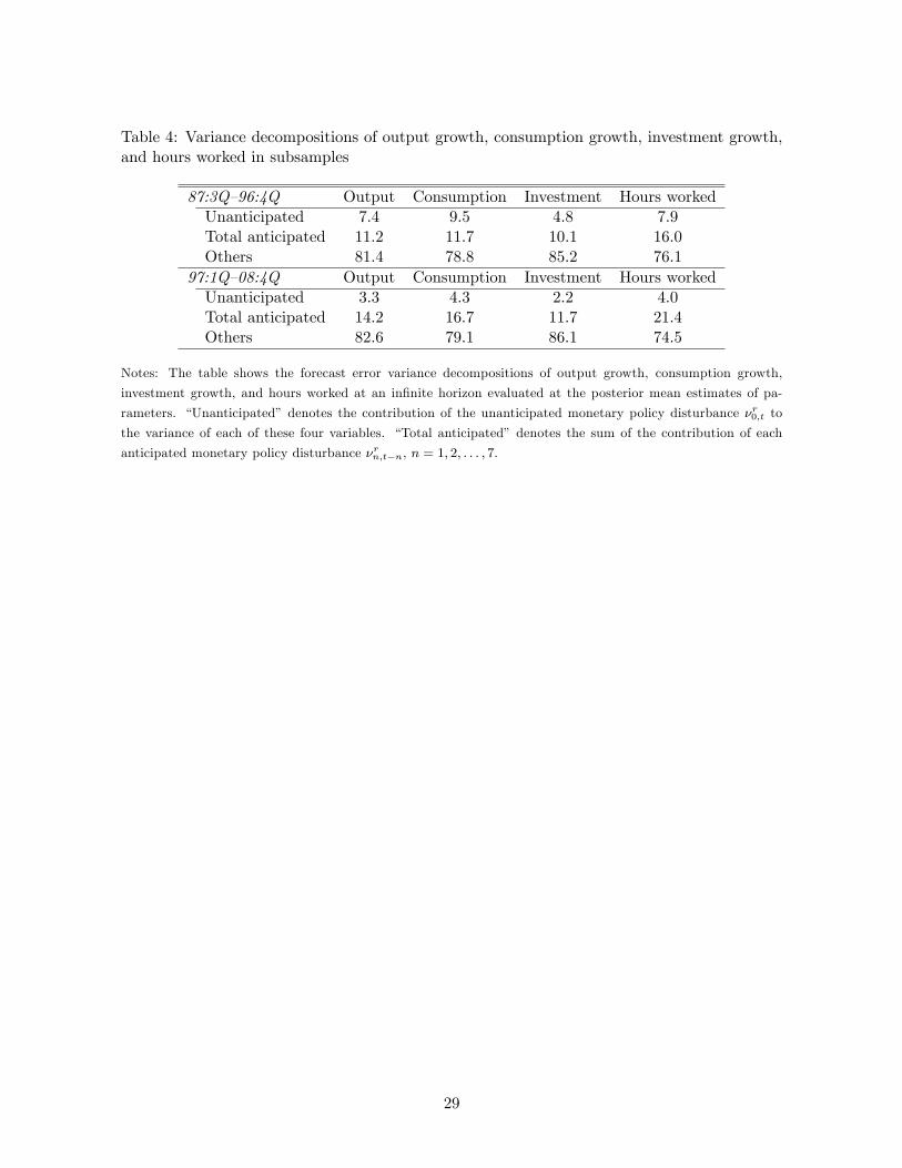
Table 4: Variance decompositions of output growth, consumption growth, investment growth,and hours worked in subsamples

87:3Q�96:4Q Output Consumption Investment Hours workedUnanticipated 7.4 9.5 4.8 7.9Total anticipated 11.2 11.7 10.1 16.0Others 81.4 78.8 85.2 76.1

97:1Q�08:4Q Output Consumption Investment Hours workedUnanticipated 3.3 4.3 2.2 4.0Total anticipated 14.2 16.7 11.7 21.4Others 82.6 79.1 86.1 74.5

Notes: The table shows the forecast error variance decompositions of output growth, consumption growth,

investment growth, and hours worked at an in�nite horizon evaluated at the posterior mean estimates of pa-

rameters. �Unanticipated� denotes the contribution of the unanticipated monetary policy disturbance �r0;t to

the variance of each of these four variables. �Total anticipated� denotes the sum of the contribution of each

anticipated monetary policy disturbance �rn;t�n, n = 1; 2; : : : ; 7.

29

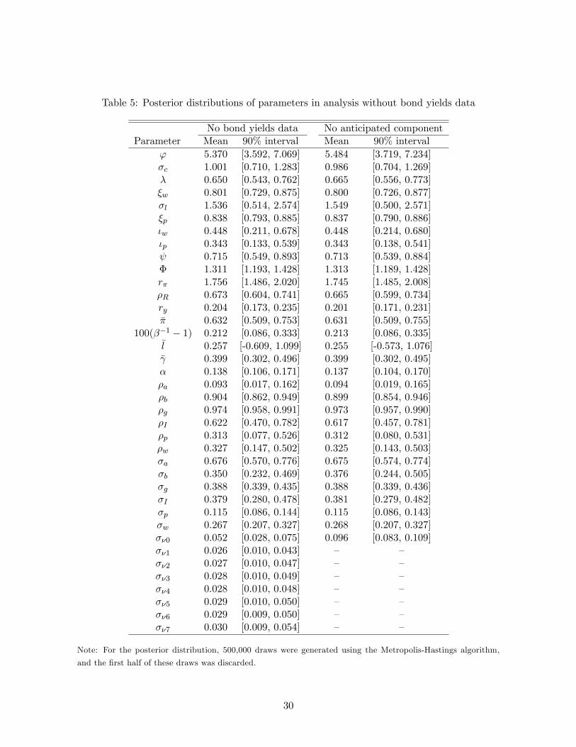
Table 5: Posterior distributions of parameters in analysis without bond yields data

No bond yields data No anticipated componentParameter Mean 90% interval Mean 90% interval

' 5.370 [3.592, 7.069] 5.484 [3.719, 7.234]�c 1.001 [0.710, 1.283] 0.986 [0.704, 1.269]� 0.650 [0.543, 0.762] 0.665 [0.556, 0.773]�w 0.801 [0.729, 0.875] 0.800 [0.726, 0.877]�l 1.536 [0.514, 2.574] 1.549 [0.500, 2.571]�p 0.838 [0.793, 0.885] 0.837 [0.790, 0.886]�w 0.448 [0.211, 0.678] 0.448 [0.214, 0.680]�p 0.343 [0.133, 0.539] 0.343 [0.138, 0.541] 0.715 [0.549, 0.893] 0.713 [0.539, 0.884]� 1.311 [1.193, 1.428] 1.313 [1.189, 1.428]r� 1.756 [1.486, 2.020] 1.745 [1.485, 2.008]�R 0.673 [0.604, 0.741] 0.665 [0.599, 0.734]ry 0.204 [0.173, 0.235] 0.201 [0.171, 0.231]�� 0.632 [0.509, 0.753] 0.631 [0.509, 0.755]

100(��1 � 1) 0.212 [0.086, 0.333] 0.213 [0.086, 0.335]�l 0.257 [-0.609, 1.099] 0.255 [-0.573, 1.076]� 0.399 [0.302, 0.496] 0.399 [0.302, 0.495]� 0.138 [0.106, 0.171] 0.137 [0.104, 0.170]�a 0.093 [0.017, 0.162] 0.094 [0.019, 0.165]�b 0.904 [0.862, 0.949] 0.899 [0.854, 0.946]�g 0.974 [0.958, 0.991] 0.973 [0.957, 0.990]�I 0.622 [0.470, 0.782] 0.617 [0.457, 0.781]�p 0.313 [0.077, 0.526] 0.312 [0.080, 0.531]�w 0.327 [0.147, 0.502] 0.325 [0.143, 0.503]�a 0.676 [0.570, 0.776] 0.675 [0.574, 0.774]�b 0.350 [0.232, 0.469] 0.376 [0.244, 0.505]�g 0.388 [0.339, 0.435] 0.388 [0.339, 0.436]�I 0.379 [0.280, 0.478] 0.381 [0.279, 0.482]�p 0.115 [0.086, 0.144] 0.115 [0.086, 0.143]�w 0.267 [0.207, 0.327] 0.268 [0.207, 0.327]��0 0.052 [0.028, 0.075] 0.096 [0.083, 0.109]��1 0.026 [0.010, 0.043] � ��2 0.027 [0.010, 0.047] � ��3 0.028 [0.010, 0.049] � ��4 0.028 [0.010, 0.048] � ��5 0.029 [0.010, 0.050] � ��6 0.029 [0.009, 0.050] � ��7 0.030 [0.009, 0.054] � �



30

Table 6: Variance decompositions of output growth, consumption growth, investment growth,and hours worked in analysis without bond yields data

Baseline Output Consumption Investment Hours workedUnanticipated 8.6 11.1 5.2 9.1Total anticipated 15.4 18.0 11.3 20.1Others 76.0 70.9 83.5 70.7

No bond yields data Output Consumption Investment Hours workedUnanticipated 0.2 0.4 0.0 0.1Total anticipated 0.5 0.6 0.3 0.7Others 99.3 99.0 99.6 99.1

No anticipated component Output Consumption Investment Hours workedUnanticipated 0.7 1.1 0.1 0.4Total anticipated � � � �Others 99.3 98.9 99.9 99.6






31

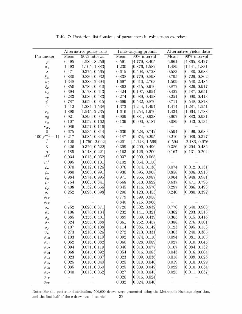
Table 7: Posterior distributions of parameters in robustness exercises

Alternative policy rule Time-varying premia Alternative yields dataParameter Mean 90% interval Mean 90% interval Mean 90% interval

' 6.495 [4.589, 8.259] 6.591 [4.779, 8.405] 6.661 [4.865, 8.427]�c 1.493 [1.105, 1.883] 1.230 [0.876, 1.582] 1.489 [1.141, 1.831]� 0.471 [0.375, 0.565] 0.615 [0.508, 0.728] 0.583 [0.480, 0.683]�w 0.880 [0.830, 0.932] 0.838 [0.779, 0.898] 0.795 [0.729, 0.862]�l 1.348 [0.283, 2.394] 1.697 [0.610, 2.763] 1.509 [0.540, 2.485]�p 0.850 [0.789, 0.910] 0.862 [0.815, 0.910] 0.872 [0.826, 0.917]�w 0.394 [0.178, 0.613] 0.424 [0.197, 0.654] 0.422 [0.187, 0.651]�p 0.283 [0.080, 0.483] 0.274 [0.089, 0.458] 0.251 [0.090, 0.413] 0.787 [0.659, 0.915] 0.699 [0.532, 0.870] 0.711 [0.548, 0.878]� 1.412 [1.284, 1.538] 1.373 [1.244, 1.494] 1.414 [1.281, 1.551]r� 1.890 [1.545, 2.235] 1.616 [1.254, 1.970] 1.434 [1.064, 1.788]�R 0.921 [0.896, 0.946] 0.909 [0.881, 0.938] 0.907 [0.883, 0.931]ry 0.107 [0.052, 0.162] 0.139 [0.090, 0.187] 0.089 [0.043, 0.134]r�y 0.086 [0.057, 0.116] � � � �� 0.675 [0.535, 0.814] 0.636 [0.528, 0.742] 0.594 [0.496, 0.689]

100(��1 � 1) 0.217 [0.085, 0.345] 0.187 [0.074, 0.295] 0.210 [0.089, 0.327]�l 0.120 [-1.750, 2.002] 0.201 [-1.143, 1.569] -0.594 [-2.186, 0.976]� 0.426 [0.326, 0.522] 0.399 [0.299, 0.496] 0.386 [0.294, 0.482]� 0.185 [0.148, 0.221] 0.163 [0.126, 0.200] 0.167 [0.131, 0.204]c1Y 0.034 [0.015, 0.052] 0.037 [0.009, 0.065] � �c2Y 0.095 [0.060, 0.131] 0.102 [0.054, 0.150] � ��a 0.070 [0.012, 0.126] 0.076 [0.014, 0.136] 0.074 [0.012, 0.131]�b 0.980 [0.968, 0.991] 0.930 [0.895, 0.968] 0.858 [0.806, 0.913]�g 0.984 [0.974, 0.995] 0.971 [0.955, 0.987] 0.964 [0.948, 0.981]�I 0.754 [0.665, 0.841] 0.668 [0.513, 0.822] 0.637 [0.471, 0.796]�p 0.408 [0.132, 0.656] 0.345 [0.116, 0.570] 0.297 [0.086, 0.493]�w 0.252 [0.096, 0.398] 0.290 [0.123, 0.453] 0.240 [0.080, 0.392]�1Y � � 0.779 [0.599, 0.958] � ��2Y � � 0.840 [0.715, 0.966] � ��a 0.752 [0.626, 0.871] 0.720 [0.602, 0.832] 0.776 [0.640, 0.908]�b 0.106 [0.078, 0.134] 0.232 [0.141, 0.321] 0.362 [0.203, 0.513]�g 0.385 [0.336, 0.431] 0.389 [0.339, 0.439] 0.365 [0.315, 0.416]�I 0.324 [0.258, 0.388] 0.361 [0.262, 0.457] 0.388 [0.276, 0.501]�p 0.107 [0.076, 0.138] 0.114 [0.085, 0.142] 0.123 [0.095, 0.153]�w 0.273 [0.216, 0.326] 0.272 [0.213, 0.331] 0.303 [0.240, 0.365]��0 0.103 [0.086, 0.119] 0.092 [0.074, 0.110] 0.094 [0.081, 0.108]��1 0.052 [0.016, 0.082] 0.060 [0.028, 0.089] 0.027 [0.010, 0.045]��2 0.094 [0.071, 0.119] 0.046 [0.013, 0.077] 0.107 [0.084, 0.132]��3 0.068 [0.045, 0.092] 0.054 [0.016, 0.083] 0.043 [0.016, 0.064]��4 0.023 [0.010, 0.037] 0.023 [0.009, 0.036] 0.018 [0.009, 0.026]��5 0.025 [0.010, 0.040] 0.025 [0.010, 0.040] 0.019 [0.010, 0.029]��6 0.035 [0.011, 0.060] 0.025 [0.009, 0.042] 0.022 [0.010, 0.034]��7 0.040 [0.013, 0.062] 0.027 [0.010, 0.045] 0.025 [0.011, 0.037]�1Y � � 0.020 [0.016, 0.024] � ��2Y � � 0.032 [0.024, 0.040] � �

Note: For the posterior distribution, 500,000 draws were generated using the Metropolis-Hastings algorithm,and the �rst half of these draws was discarded. 32

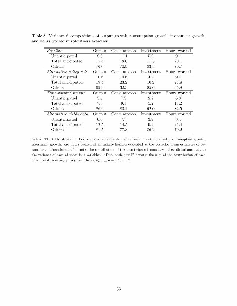
Table 8: Variance decompositions of output growth, consumption growth, investment growth,and hours worked in robustness exercises

Baseline Output Consumption Investment Hours workedUnanticipated 8.6 11.1 5.2 9.1Total anticipated 15.4 18.0 11.3 20.1Others 76.0 70.9 83.5 70.7

Alternative policy rule Output Consumption Investment Hours workedUnanticipated 10.6 14.6 4.2 9.4Total anticipated 19.4 23.2 10.2 23.8Others 69.9 62.3 85.6 66.8

Time-varying premia Output Consumption Investment Hours workedUnanticipated 5.5 7.5 2.8 6.3Total anticipated 7.5 9.1 5.2 11.2Others 86.9 83.4 92.0 82.5

Alternative yields data Output Consumption Investment Hours workedUnanticipated 6.0 7.7 3.9 8.4Total anticipated 12.5 14.5 9.9 21.4Others 81.5 77.8 86.2 70.2






33

1.5

1

0.5

0

0.5

1

1.5

87 | 88 | 89 | 90 | 91 | 92 | 93 | 94 | 95 | 96 | 97 | 98 | 99 | 00 | 01 | 02 | 03 | 04 | 05 | 06 | 07 | 08

Unanticipated component

Anticipated components

Monetary policy disturbances

(%)

Figure 1: Historical decomposition of monetary policy disturbances

Notes: The �gure shows the historical decomposition of monetary policy disturbances evaluated at the poste-

rior mean estimates of parameters. �Unanticipated component� denotes the contribution of the unanticipated

component �r0;t to the whole monetary policy disturbances. �Anticipated components�denotes the sum of the

contribution of each anticipated component �rn;t�n, n = 1; 2; : : : ; 7.

34

1.5

1

0.5

0

0.5

1

1.5

87 | 88 | 89 | 90 | 91 | 92 | 93 | 94 | 95 | 96 | 97 | 98 | 99 | 00 | 01 | 02 | 03 | 04 | 05 | 06 | 07 | 08




(%)

Figure 2: Historical decomposition of monetary policy disturbances estimated without bondyields data





35

1.5

1

0.5

0

0.5

1

1.5

87 | 88 | 89 | 90 | 91 | 92 | 93 | 94 | 95 | 96 | 97 | 98 | 99 | 00 | 01 | 02 | 03 | 04 | 05 | 06 | 07 | 08




(%)

Figure 3: Historical decomposition of monetary policy disturbances estimated with alternativespeci�cation of monetary policy rule





36

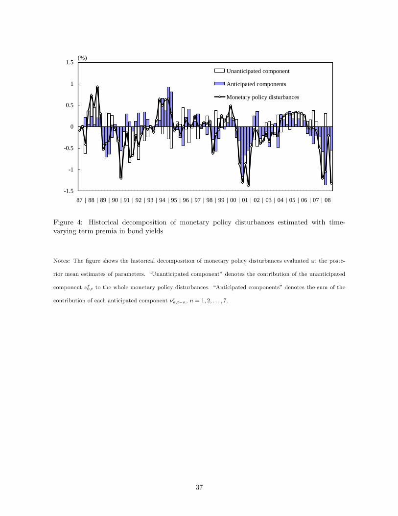
1.5

1

0.5

0

0.5

1

1.5

87 | 88 | 89 | 90 | 91 | 92 | 93 | 94 | 95 | 96 | 97 | 98 | 99 | 00 | 01 | 02 | 03 | 04 | 05 | 06 | 07 | 08




(%)

Figure 4: Historical decomposition of monetary policy disturbances estimated with time-varying term premia in bond yields





37

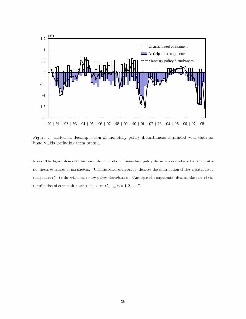
2

1.5

1

0.5

0

0.5

1

1.5

90 | 91 | 92 | 93 | 94 | 95 | 96 | 97 | 98 | 99 | 00 | 01 | 02 | 03 | 04 | 05 | 06 | 07 | 08




(%)

Figure 5: Historical decomposition of monetary policy disturbances estimated with data onbond yields excluding term premia





38

changes in the federal reserve communication strategy · pdf filechanges in the federal...

Documents