changes in the size distribution of us banks - federal reserve

Changes in the SizeDistribution of U.S. Banks:1960–2005

Hubert P. Janicki and Edward Simpson Prescott

I n 1960, there were nearly 13,000 independent banks. By 2005, the numberhad dropped in half, to about 6,500. In 1960, the ten largest banks held21 percent of the banking industry’s assets. By 2005, this share had

grown to almost 60 percent. A great deal of these changes started during thederegulation of the 1980s and 1990s. (Figures 1 and 2 report the time pathsfor these two measures.)

By any measure, these numbers represent a dramatic change in the banksize distribution over the 1960–2005 period. This article documents theextent of this change. It also documents the change in bank size dynamics,that is, the entry and exit of banks and the movement of banks through thesize distribution. During this period, new banks formed, many more exited,either because of failure or merger, and many others changed in their size.For example, of the ten largest banks in 1960, only three were still among thetop ten largest in 2005.1

We document these facts because they are an important step in developinga theory of bank size distribution. Although we do not provide one, sucha theory would be valuable because it could be used to answer importantquestions such as: How costly were the pre-1980 limits on bank size? How

Hubert P. Janicki is a graduate student in economics at Arizona State University. The viewsexpressed in this article are those of the authors and not necessarily those of the FederalReserve Bank of Richmond or the Federal Reserve System. The authors would like to thankHuberto Ennis, Yash Mehra, Andrea Waddle, and John Weinberg for helpful comments.

1 The ten largest banks in 1960 were Bank of America, Chase Manhattan Bank, First NationalCity Bank of New York, Chemical Bank New York Trust Company, Morgan Guaranty Trust Com-pany, Manufacturer’s Hanover Trust Company, Bank of California, Security First National Bank,Banker’s Trust Company, and First National Bank of Chicago. At the end of 2005, only three ofthese banks still existed: Bank of America, Citigroup (formerly National City Bank of New York),and JP Morgan Chase (an amalgamation of many of the banks listed above).

Federal Reserve Bank of Richmond Economic Quarterly Volume 92/4 Fall 2006 291

292 Federal Reserve Bank of Richmond Economic Quarterly

Figure 1 Total Number of Independent Banks

1960 1965 1970 1975 1980 1985 1990 1995 2000 2005

7,000

8,000

9,000

10,000

11,000

12,000

13,000N

um

be

r o

f B

an

ks

Year

Notes: All banks and bank holding companies that are under a higher level holding com-pany are treated as a single independent bank. Section 3 gives a more precise definitionof an independent bank.

will the bank size distribution continue to evolve? And will there be moreconcentration? If so, should policy do anything about it?

Our analysis of the size distribution emphasizes fitting the data to thelognormal and Pareto distributions. These distributions are utilized becausethey are commonly used to describe skewed distributions and frequently havebeen used to describe firm size distribution. As we will demonstrate, thelognormal poorly fits the upper right tail of the size distribution. The Paretodistribution fits better with this part of the distribution, but the quality of thefit is much better before deregulation.

We examine bank size dynamics along several dimensions. First, wedetermine whether the data satisfies Gibrat’s Law, that is, whether growthis independent of firm size. We find that Gibrat’s Law is a good descrip-tion of the data during the 1960s and 1970s, before deregulation, but not agood description afterward. After the 1970s, large banks grew faster thansmall banks, though more so in the 1980s and 1990s than they did during the

H. P. Janicki and E. S. Prescott: Bank Size Distribution 293

Figure 2 Market Shares of Ten Largest Banks

1960 1965 1970 1975 1980 1985 1990 1995 2000 2005

0.20

0.25

0.30

0.35

0.40

0.45

0.50

0.55

Fr

actio

ns o

f Tot

al

Year

AssetsLoansDepositsEmployees

Notes: The definition of a bank is given in Section 3. Data on number of employeesstarts in 1969.

2000–2005 period. Second, we document that entry into banking was re-markably stable over the entire period. Entry is cyclical but averages about1.5 percent of total operating banks. Finally, we calculate transition matrices,that is, the probability a bank will move from one size category to another,over each of the decades. Following Adelman (1958) and Simon and Bonini(1958), we use these transition probabilities and the entry data from 2000–2005to forecast continued changes in the size distribution. The forecast predictsa continued decline in the total number of banks, but at a much slower ratethan in the 1980s and 1990s, followed by a leveling off in the decline. It alsopredicts that there will still be a large number of small banks as well as a siz-able number of mid-size banks. If the present trends continue, the transitionin banking that began in the 1980s is slowing down and coming to an end.

1. LITERATURE

In many industries, the distribution of firm size is highly skewed to the right,that is, there are many small firms and a few large ones. One distribution thathas this characteristic and is frequently used to describe firm size distribution


is the lognormal distribution. A random variable is lognormally distributed ifthe logarithm of the random variable is normally distributed.2

Early studies of firm size distribution, namely Gibrat (1931), found thatthe lognormal distribution fit the empirical data fairly well. Gibrat (1931)also found evidence that firm growth was independent of firm size. Thislatter finding, often called Gibrat’s Law or the Law of Proportionate Effect,was important because a statistical process that satisfies it would generate alognormal distribution in the long run.

Later studies have found mixed support for Gibrat’s findings. In particu-lar, studies in the 1980s found that the proportional rate of growth of a firmconditional on survival decreases in size. Sutton (1997) is a good survey ofthese results.

Another category of distributions used to fit the size distribution is basedon the power law. This category takes the form

f (x) = cx−α,

where x > 0 and c > 0. In economics, the Pareto distribution is a power lawdistribution often used to describe highly skewed data.3 It is similar to thelognormal, but with a thicker right tail.

Power law distributions have been used in the sciences to fit data in a widevariety of applications. Newman (2005) surveys various applications of thepower law, including studies of word frequency, magnitude of earthquakes,diameter of moon craters, intensity of solar flares, and population of cities.One property observed in many applications is that the size of the r-th largestobservation is inversely proportional to its rank.4 It is observed so frequentlythat it is called Zipf’s Law. Like the lognormal distribution, Zipf’s Law can begenerated with appealing assumptions on the dynamics. For example, Simonand Bonini (1958) study entry dynamics by assuming a constant probabilityof entry and show that the distribution follows a power law in the upper tail.See Gabaix (1999) for a detailed study of Zipf’s Law.

2 The probability density function of a lognormal distribution is

f (x) = 1

σ√

2π

1

xe−(log(x)−μ)2/(2σ2),

where x > 0, μ and σ are the mean and standard deviation, respectively, of the natural log of x.3 The probability density function of a Pareto distribution is

f (x) = kxkminx−(k+1)

where x > xmin, xmin > 0 and k > 0. The Pareto distribution is usually expressed as theprobability that random variable X is greater than x, that is, Prob(X ≥ x) = xk

minx−k , which is

also a power law.4 Formally, xr = cr−α , where observation xr has rank r , c is a constant, and α is close to

1. We solve for r , normalize the equation by dividing by N (where the N th ranked observationis xmin) and simplify to obtain the counter cumulative function: r/N = 1 − F(x) = (xmin/x)1/α .This is the Pareto distribution with coefficient k = 1/α.


Whether Zipf’s Law fits U.S. firm size data is a matter of some debate.Using 1997 U.S. census data, Axtell (2001) finds that it fits the firm sizedistribution. Using a different data set, however, Rossi-Hansberg and Wright(2006) find that it does not fit so well. They also find that establishment growthand exit rates decline with size.

The banking literature has long been interested in the size distribution ofbanks, partly because of the large degree to which laws and regulations limitedbank size. Recent studies include Berger, Kashyap, and Scalise (1995), Ennis(2001), and Jones and Critchfield (2005).

While the banking literature has long noted that bank size distribution isskewed, it has not typically tried to fit this using the previously mentionedcategory of distributions. This absence has made it difficult to compare banksize distribution with that of other industries.

There is part of this literature, however, that tests for Gibrat’s Law inthe banking industry but for smaller samples than those used in this study.Alhadeff and Alhadeff (1964) analyze growth in assets of the 200 largest U.S.banks between 1930–1960 and find the largest banks grew more slowly thanthe banking system itself. They find, however, that the top banks that survivedthroughout the sample period grew faster than the system as a whole andattribute this to mergers among the largest banks. Rhoades and Yeats (1974)analyze growth among U.S. banks by deposits for 1960–1971 and find that thelargest banks grew more slowly than the whole banking system. In a studyof the 100 largest international banks from 1969 to 1977 by assets, Tschoegl(1983) finds that growth rates of banks are roughly independent of size, but thatgrowth rates exhibit positive serial correlation. Saunders and Walter (1994)use international data for the 200 largest banks for the 1982–1987 period andreject Gibrat’s Law, finding that the smaller banks grow faster than larger banksin terms of assets. More recently, Goddard, McKillop, and Wilson (2002) findevidence that during the 1990s in the United States, large credit unions grewfaster than their smaller counterparts.

As we discussed, the firm growth results are important because they ul-timately determine the distribution of firm sizes. One interesting strand inthe literature calculates a Markov transition matrix of movement between sizecategories and then calculates stationary size distributions. Early examplesinclude Hart and Prais (1956), Simon and Bonini (1958), and the study of thesteel industry by Adelman (1958). The only study that we are aware of thatapplies this technique to banking is Robertson (2001).

More recently, the literature has attempted to generate firm size dynam-ics, and ultimately a size distribution, from models of maximizing behaviorof firms. Sutton (1997) surveys several such models. One paper in this liter-ature is the learning model of Jovanovic (1982), in which new firms receiveproductivity shocks, learn about them over time, and then decide whether tocontinue or exit. Another prominent example is Hopenhayn (1992).


2. LEGAL AND REGULATORY LIMITS ON BANK SIZE

Describing bank size distribution is particularly important because of the manylegal and regulatory limits on bank size that existed through the 1970s andwere removed during the 1980s and 1990s. As we will see, the removal ofthese barriers coincide with dramatic changes in size dynamics and the sizedistribution.

In 1960, banks could not branch across state lines and some states evenforbade branching within a state.5 The 1966 Douglas Amendment to the 1956Bank Holding Company Act allowed interstate banking only with expressedauthorization by participating states. However, no state allowed interstatebanking at the time and the amendment was not even exercised until 1978when Maine allowed out-of-state bank holding companies (BHCs) to operatewithin the state.6 Over the next 12 years, many of the intrastate and interstaterestrictions were removed by the states.7

The remaining interstate banking restrictions were removed by theRiegle-Neal Interstate Banking and Branching Efficiency Act of 1994. Theact permitted bank holding companies to acquire banks in any state and, be-ginning in 1997, allowed interstate bank mergers. (See Kane [1996] for asummary of the act.) More recently, the Gramm-Leach-Bliley Act of 1999allowed banks to engage in nonbanking financial activities such as insurance.

3. THE DATA

Many banks operate under a bank holding company structure. A bank holdingcompany is a legal entity that i) directly or indirectly owns at least 25 percentof the bank’s stock, ii) controls the election of a majority of a bank’s directors,or iii) is deemed to exert controlling influence of bank policy by the FederalReserve (Spong 2000). Many bank holding companies have multiple banksand even other holding companies under their control. Historically, this legalorganization was used to avoid some of the restrictions on branching (Mengle1990). In many cases, a bank holding company would operate many activi-ties jointly. For this reason, we follow Berger, Kashyap, and Scalise (1995)and treat all banks and bank holding companies under a higher level holding

5 The 1927 McFadden Act forbade interstate branching by federally chartered banks. Later,the Federal Reserve extended the ruling to include all state-chartered banks that are regulated bythe Federal Reserve.

6 There were some means around these restrictions. For example, the 1956 Bank HoldingCompany Act did not limit the location of nonbank subsidiaries of bank holding companies, sosome banks had a cross-state network of nonbranch offices that would specialize in activities likelending. Also, some exemptions were allowed for the acquisition of insolvent banks from govern-ment deposit insurance funds (Kane 1996).

7 Jayaratne and Strahan (1997) list when states removed restrictions to interstate banking andintrastate branching.


company as a single independent banking enterprise. For convenience, wewill typically refer to each of these entities as a bank.

Data on banks are taken from the Reports on Condition and Income (the“Call Report”) collected by federal bank regulators. We use fourth quarterdata on all commercial banks in the United States. We look specifically atcommercial banks and exclude savings banks, savings and loan associations,credit unions, investment banks, mutual funds, and credit card banks. Indi-vidual commercial banks that belong to a holding company are then groupedaccording to a unique bank holding company regulatory number, and theirassets, deposits, loans, and employees are summed and replaced by one entryin our data set. Our data set, therefore, tracks bank holding companies andindependent commercial banks not affiliated with a holding company. It doesnot distinguish between a merger and a failure. Both events are treated as anexit.

We use four measures of bank size. The first is commercial bank assets.For this variable, we have data from 1960–2005. Prior to 1969, we only havedomestic holdings, but after 1969, we have foreign and domestic holdings.The next two size measures are domestic holdings of deposits and loans. Forboth of these variables, we have data from 1960–2005. The final size measureis the number of domestic employees.8 For this last measure, we only havedata for 1969–2005. Assets and loans are adjusted to include off-balance-sheetitems starting in 1990. (See the Appendix for details.) All the variables areadjusted for the total aggregate size of that variable in each year. In particular,firm size data are converted into market share numbers for that year and thenmultiplied by the total quantity in the banking industry of that variable in2004. The market share adjustment facilitates comparison across years, whilethe scaling by 2004 aggregate quantities gives a sense of the size in terms ofrecent quantities.

4. THE SIZE DISTRIBUTION

The size distribution of banks has always been skewed, but it has become moreso since the 1960s. Figure 3 shows the distribution of assets for 1960, 1980,and 2005. Each year is normalized by the total assets in that year relativeto 2004 so that the distributions are comparable over time. The distributionis plotted on a log scale. Because the size distribution is so skewed to theright, the log scale—or something similar—is needed to fit all the banks onthe graph.

Figure 3 demonstrates that there are a large number of small banks anda few large banks. As is evident, there is a shift in the distribution to the left

8 The Call Report counts employees in terms of full-time equivalents.


Figure 3 Change in Bank Size Distribution Over Time

101 102 103 104 105 1060.00

0.01

0.02

0.03

0.04

0.05

0.06

P

roba

bilit

y196019802005

Assets (Millions USD, 2004) Log Scale

Notes: Each line is a probability distribution of bank size as measured by assets for agiven year.

over time. Since we have scaled assets in each year to be the same scale, thischange means that a higher fraction of the assets are being held by the smallnumber of large banks, as indicated earlier in Figure 2.

Visually, the graphs suggest that the distribution might be accurately rep-resented by a lognormal distribution. Figure 4 reports the actual distributionand an estimated lognormal distribution for assets in 2005, where the log-normal has parameters μ and σ 2 obtained from the 2005 data set. However,the distribution fails the Kolmogorov-Smirnov test for goodness-of-fit. Thisis true for almost all the years in the data set, as well as for the other sizemeasures.

The estimated lognormal distribution does a particularly poor job of fittingthe right tail of the distribution. This is hard to see in Figure 4 because of thesmall number of large banks. The fit at the right tail is better seen if we usea rank-frequency, or Zipf plot. For a power law distribution plotted on a logscale, this type of graph has the valuable property that the slope will be linear.For example, let xr = cr−α, where r is the rank of a variable. Taking the


Figure 4 Size Distribution of Banks in 2005

101

102

103

104

105

106

0.00

0.01

0.02

0.03

0.04

0.05

0.06

Assets (Millions USD, 2004) Log Scale

Pro

babi

lity

DataLognormal, ( =11.7234, =1.8727)2μ σ

Notes: The parameters μ and σ are the mean and standard deviation, respectively, of thenatural log of assets. The lognormal distribution is calculated using these parameters.

logarithm of both sides, we obtain the equation,

ln(xr) = ln(c) − αln(r).

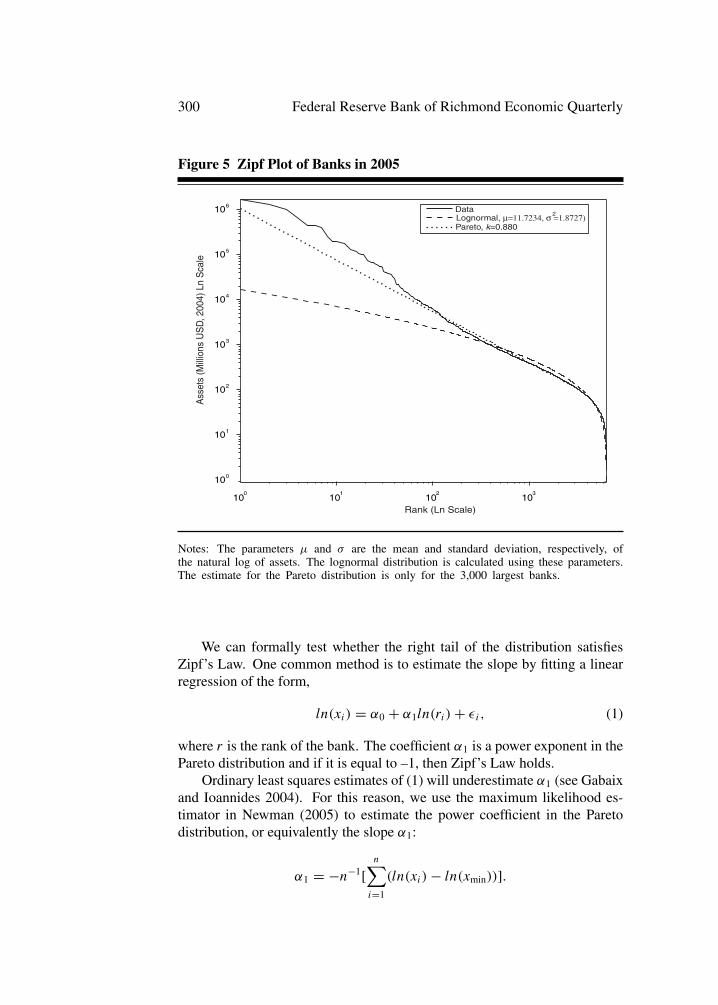
If α = 1, then Zipf’s Law holds.Figure 5 is a Zipf plot for the bank size distribution in 2005.9 It plots the

data and the lognormal distribution using the sample mean and variance.Figure 5 demonstrates that the lognormal distribution underestimates the

density of the right tail (which is the left side in the Zipf plot). Indeed,if the plot is linear, we know that the right tail of the distribution of bankholding companies can be better approximated by the Pareto distribution.Note, however, that only the right tail of the distribution—which correspondsto the left side of the figure—appears to fit Zipf’s Law. That is, the distributionof bank holding companies seems to be lognormally distributed with a Pareto-distributed tail.

9 Zipf plots for different size measures look very similar.


Figure 5 Zipf Plot of Banks in 2005

100

101

102

103

100

101

102

103

104

105

106

Rank (Ln Scale)

Ass

ets

(Mill

ions

US

D, 2

004)

Ln

Sca

le

Lognormal, μ=11.7234, σ =1.8727)2

Pareto, k=0.880

Data

Notes: The parameters μ and σ are the mean and standard deviation, respectively, ofthe natural log of assets. The lognormal distribution is calculated using these parameters.The estimate for the Pareto distribution is only for the 3,000 largest banks.

We can formally test whether the right tail of the distribution satisfiesZipf’s Law. One common method is to estimate the slope by fitting a linearregression of the form,

ln(xi) = α0 + α1ln(ri) + εi, (1)

where r is the rank of the bank. The coefficient α1 is a power exponent in thePareto distribution and if it is equal to –1, then Zipf’s Law holds.

Ordinary least squares estimates of (1) will underestimate α1 (see Gabaixand Ioannides 2004). For this reason, we use the maximum likelihood es-timator in Newman (2005) to estimate the power coefficient in the Paretodistribution, or equivalently the slope α1:

α1 = −n−1[n∑

i=1

(ln(xi) − ln(xmin))].


Table 1 Zipf’s Law: Maximum Likelihood Estimates

1960 1970 1980 1990 2005–α1 SE –α1 SE –α1 SE –α1 SE –α1 SE

Assets 1.001 0.001 1.030 0.001 1.018 0.001 1.017 0.001 1.136 0.001Deposits 0.998 0.001 1.016 0.001 0.983 0.001 0.982 0.001 1.092 0.001Loans 1.028 0.001 1.051 0.001 1.007 0.001 1.082 0.001 1.187 0.001Employees – – 1.022 0.065 1.031 0.073 1.005 0.084 1.052 0.096

Notes: The estimates are reported as −α1.

The maximum likelihood estimates for several different years are reported inTable 1.10 We restrict the estimates to the tail by limiting the sample to thelargest 3,000 banks for each year. Although they are not identical across years,they broadly support Zipf’s Law in the upper tail, but the results are sensitiveto the cutoff.

The worst fit inTable 1 is in 2005. This can be seen in Figure 5. The straightline in Figure 5 graphs the power distribution for the maximum likelihoodestimate based on the 3,000 largest banks. The distribution is a straight linewith slope –1.136. The slope is too high for Zipf’s Law. Furthermore, theslope is high because the larger banks are larger than predicted by Zipf’s Law,though this is less true for the largest.

In contrast, the fit for assets in 1960 is excellent. Figure 6 is a Zipf plot forassets in 1960. The distribution is a straight line with slope –0.999, practicallythe same as in Zipf’s Law.

The estimates for assets in 1970, 1980, and 1990 are similar, but this hidesan important difference. The year 1970 is similar to 1960 in that many of thelargest banks are smaller in size than predicted by the estimate. In 1980, thispattern changes to one where the largest banks are larger than predicted. Thedifferences in the predictions for the largest banks are even larger in 1990 andlook similar to that of 2005 (see Figure 5).

To summarize, only the right tail can reasonably be considered to be fittedby Zipf’s Law, and the fit depends on the year. It does well in 1960, but startingin 1980 Zipf’s Law predicts that the largest banks will be smaller than in thedata. The lognormal distribution poorly fits the size of the largest banks butbetter fits the small banks.

10 We calculate standard errors using the method outlined in Gabaix and Ioannides (2004).


Figure 6 Zipf Plot of Banks in 1960

100

101

102

103

104

101

102

103

104

105

106

A

sset

s (M

illio

ns U

SD

, 200

4) L

n S

cale

Rank (Ln Scale)

Lognormal, μ=12.1774, σ =1.4948)2

Pareto, k=0.999

Data

Notes: The parameters μ and σ are the mean and standard deviation, respectively, ofthe natural log of assets. The lognormal distribution is calculated using these parameters.The estimate for the Pareto distribution is only for the 3,000 largest banks.

5. DOES GIBRAT’S LAW HOLD FOR BANKS?

Gibrat’s Law states that firm size growth is independent of firm size. For ourfirst test of this law, we fit the following linear equation,

ln(xit+1) = β0 + β1ln(xit ) + εit , (2)

where xit is the size measure (assets, employees, etc.) of bank i at time t . Acoefficient value of β1 = 1 means that growth is independent of size.

We estimated (2) over each decade and over 2000–2005 using ordinaryleast squares. We only considered banks in the sample that were around at thebeginning and end of the estimation period. Those that exited were droppedfrom the sample.11 The estimates are reported in Table 2.

11 Sometimes the literature includes exiting banks and sometimes it does not. See Sutton(1997) for more information. To reduce survivorship bias, we also estimated equation (2) overeach year and found similar results to those reported in Table 2.


Table 2 Gibrat’s Law: Estimates

1960–1969 1970–1979 1980–1989 1990–1999 2000–2005

Assetsβ0 0.143 (0.031) 0.574 (0.034) 0.043 (0.057) –0.187 (0.074) 0.015 (0.061)β1 0.987 (0.003) 0.953 (0.003) 1.011 (0.005) 1.024 (0.006) 0.998 (0.005)R2 0.929 0.915 0.847 0.823 0.869

Depositsβ0 0.435 (0.030) 1.004 (0.033) 0.131 (0.058) 0.654 (0.075) 0.379 (0.063)β1 0.971 (0.003) 0.929 (0.003) 0.999 (0.005) 0.972 (0.007) 0.970 (0.005)R2 0.923 0.902 0.826 0.787 0.847

Loansβ0 0.545 (0.037) 1.368 (0.039) 0.000 (0.071) 0.635 (0.074) 0.444 (0.069)β1 0.960 (0.003) 0.901 (0.003) 0.993 (0.006) 0.964 (0.007) 0.962 (0.006)R2 0.889 0.870 0.767 0.782 0.812

Employeesβ0 – – –0.021 (0.012) 0.240 (0.016) 0.284 (0.022) 0.101 (0.017)β1 – – 1.006 (0.003) 1.001 (0.004) 1.008 (0.006) 0.994 (0.004)R2 – 0.897 0.862 0.829 0.900

Notes: The table provides ordinary least squares estimates of equation (2) for each sampleperiod. Standard errors are in parentheses. Numbers in bold are the slope estimates ofthe effect of firm size on growth. An estimate close to one is consistent with Gibrat’sLaw.

The estimates in Table 2 are close to one for all the decades and variables.While broadly supportive of Gibrat’s Law, these estimates put a great deal ofemphasis on small banks because they comprise most of the sample. For thisreason, we broke the sample into different size categories and then calculatedthe annualized growth rates over the same periods for banks in each category.As before, we only considered banks that survived. Figure 7 reports the growthrates for assets, deposits, and loans.12

Just as in Table 2, growth measures do not vary much with size in the1960s and 1970s.13 In the 1980s and 1990s, however, the numbers in Figure7 present a different picture than the estimates in Table 2. As demonstratedby the figure, the largest banks clearly grew faster than the small banks. Thisis also true for the 2000–2005 period, but the effect is less pronounced.

12 A figure showing employee growth rates is excluded because the growth rates jump aroundsignificantly and do not show any clear patterns.

13 We have also calculated annual growth rates over each period and then averaged them toget a similar figure. (Over the 1960–1969 period, for example, this meant calculating the 1960–1961, 1961–1962, etc., growth rates and then averaging them.) The results are similar.


Figure 7 Annualized Growth Rates by Size Categories

10210

310

410

5-2

0

2

4

6

8

10

102

103

104

-2

0

2

4

6

8

10

102

103

104

105

-2

0

2

4

6

8

10

An

nu

aliz

ed

Gro

wth

(%

)

Assets in Millions (Log Scale)

Deposits in Millions (Log Scale)

Loans in Millions (Log Scale)

1960-19691970-19791980-19891990-19992000-2005

An

nu

aliz

ed

Gro

wth

(%

)A

nnu

aliz

ed

Gro

wth

(%

)

1960-19691970-19791980-19891990-19992000-2005

1960-19691970-19791980-19891990-19992000-2005

Notes: The size measure is broken into seven size categories and then average annualizedgrowth rates are reported for each category.


Gibrat’s model that yields the law of proportionate effect assumes thatgrowth rates are not persistent over time. To check the validity of this as-sumption, we calculate the correlation of growth rates for surviving banks ineach decade. We find that correlations of growth rates for all variables arevery low. In the 1960s, it is 0.0610; in the 1970s, it is 0.0331; in the 1980s, itis 0.0691; in the 1990s, it is 0.0722; and after 2000, it is 0.1617. Correlationcoefficients of growth in the remaining variables are of similar magnitude.

To conclude, growth rates appear to be independent of size in the 1960sand 1970s, but they are positively related to size in the 1980s and 1990s. Inthe 2000–2005 period, the growth rates are also higher for the largest banks,but less so than in the previous two decades. It appears that the 1960s and1970s were relatively stationary periods, but the 1980s and 1990s were along transition period, no doubt due to the legal, regulatory, and technologicalchanges of the period. Finally, the 2000–2005 period appears to be the end ofthe transition, as the size dynamics seem to be returning slowly to the numbersof the 1960s and 1970s. Of course, this conclusion is tentative because trendscalculated from five years of data can easily be transitory.

6. ENTRY AND EXIT

Despite the large number of banks that have exited the industry over the last45 years, there has been a consistent flow of new bank entries. The numberof entries and exits (including mergers) expressed as a fraction of the bankingpopulation is reported in Figure 8.

Visually, it is apparent that the flow of new banks is a relatively constantfraction of the banking population. To check this, we estimated a linear timetrend of the number of entries as a fraction of the number of banks operating.Specifically we estimated the equation,

yt = γ 0 + γ 1t + εt,

where yt is the fraction of entries per year and t is the time trend. The ordinaryleast squares estimates are γ 0 = 0.0145 (0.0018), γ 1 = 0.0001 (0.0001) withR2=0.0612. Standard errors are in parentheses. There is no time trend in theflow of new banks, though there is a significant amount of cyclical variation.

The fraction of banks that exit varied a great deal over time. There wasa significant increase starting in the 1980s and, except for a short dip in theearly 1990s, the high level continued through the late 1990s. No doubt muchof this exit was due to mergers, particularly those that occurred in the 1990s,but our data does not allow us to distinguish between these two sources ofexit. It is only in the last five years that the rate of exit seems to slow down.

It is striking that despite the huge number of bank exits starting in the1980s, entry remained strong throughout the entire period. Interestingly, itis virtually uncorrelated with exit. For example, the correlation between exit


Figure 8 Fraction of Banks that Enter and Exit by Year

1965 1970 1975 1980 1985 1990 1995 2000 2005

-0.06

-0.05

-0.04

-0.03

-0.02

-0.01

0.00

0.01

0.02

Fra

ctio

n of

Ent

ries

and

Exi

ts

Year

EntriesExits/Mergers

Notes: The chart reports the gross flow of banks that enter and exit expressed as afraction of banks in each year.

and entry for the 1985–2005 period is only –0.07. This evidence means that atheory of the bank size distribution needs to be able to generate robust entry,even when the total number of banks is declining.

7. THE DYNAMICS OF THE SIZE DISTRIBUTION

In this section, we use the information previously documented—the size dis-tribution at a point of time, entry and exit rates, and bank dynamics—to makeforecasts of what will happen to the size distribution. We also perform coun-terfactual experiments such as what would have happened to the bank sizedistribution if the dynamics had not changed. The purpose of these exercisesis to develop a sense of how changes in size dynamics have mattered for thesize distribution.

To make these calculations, we do not use growth rates at the individualbank level. Instead, we do something similar by constructing a simple Markovchain model following Adelman (1958). A Markov chain model splits the


Figure 9 Projected Number of Banks

1960 1965 1970 1975 1980 1985 1990 1995 2000 2005 2010

5,000

6,000

7,000

8,000

9,000

10,000

11,000

12,000

13,000

N

umbe

r of

Ban

ks

Year

DataTransition Matrix 1960-1969Transition Matrix 1970-1979Transition Matrix 1980-1989Transition Matrix 1990-1999Transition Matrix 2000-2005

Notes: Each projection is made by taking the transition matrix estimated over a givenperiod and then calculating the total number of banks that would operate after the lastyear in that given period.

banks into a finite number of size categories. Probabilities of moving betweensize categories are summarized with a Markov, or transition, matrix. A Markovmatrix is a square matrix, P , where element Pij specifies the probability a bankthat starts in size category i will move into size category j in the next period.

A Markov model allows for straightforward predictions about changes toa size distribution. For example, if the size distribution at time t is st , then thesize distribution at time t + n is

st+n = P nst .

If a Markov model has the property that a bank starting in any categoryhas a positive probability of moving to any other size category in a finitenumber of periods, then several useful theorems apply. First, there exists a


Table 3 Transition Matrix Size Categories (Scaled Dollars)

Size Categories Assets1 <100m2 100m-500m3 500m-1b4 1b-5b5 5b-10b6 10b-50b7 50b<

Notes: A list of size categories used in the Markov model. In all years, data are convertedinto market share numbers and then multiplied by the total quantity of assets in 2004.

stationary distribution, that is, there exists s such that s = Ps.14 Second,the stationary distribution is unique and independent of the initial distributionof banks. Therefore, regardless of the initial distribution, if the transitionmatrix, P , is repeatedly applied to the distribution, then the size distributionwill approach the unique stationary distribution.

We construct seven different size categories. These are listed in Table 3.All the data are scaled as we discussed earlier to make it possible to compareacross years. We also include an eighth category that represents banks that areinactive. New banks come from this category and exiting banks move into it.We calculate the number of banks in each of the seven active categories. Forthe inactive banks, we assume that there is a large pool of 100,000 potentialentries.

Our transition matrix is calculated by counting the fraction of banks thatmove from size category i to j each year over the specified time period. Entryrates are calculated so that a constant fraction of potential banks enter.

For our first exercise, we use the transition matrices estimated over severalranges of time periods to forecast the aggregate number of banks in the in-dustry. We estimate several transition matrices and make predictions to 2013.The results are illustrated in Figure 9. For each period, we calculate the tran-sition matrix and then forecast the change in the total number of banks as ifthe transition probabilities had not changed from that time period forward.This exercise is similar to one in Jones and Critchfield (2005), although ourmethodology is very different. An advantage of our Markov chain model isthat we have information on the entire distribution at each point in Figure 9.

As is clear from the earlier analysis, as well as from Figure 9, the sizedynamics changed significantly over this period. Nevertheless, the exercise

14 Let sj be the fraction of banks in size category j . The stationary distribution s is thesolution to the set of equations s = Ps and

∑j sj = 1.


Table 4 Stationary Distribution of Banks by Assets

Size 1960–1969 1970–1979 1980–1989 1990–1999 2000–2005Categories 1969 SS 1979 SS 1989 SS 1999 SS 2005 SS

1 0.333 0.357 0.379 0.439 0.379 0.471 0.440 0.523 0.480 0.5402 0.504 0.516 0.492 0.485 0.488 0.435 0.436 0.377 0.399 0.3633 0.085 0.076 0.064 0.044 0.067 0.049 0.061 0.051 0.060 0.0504 0.060 0.042 0.046 0.021 0.043 0.027 0.044 0.037 0.043 0.0335 0.008 0.004 0.007 0.003 0.008 0.005 0.006 0.004 0.008 0.0066 0.009 0.005 0.010 0.005 0.010 0.007 0.007 0.005 0.006 0.0057 0.002 0.000 0.002 0.003 0.005 0.007 0.005 0.002 0.005 0.003

Notes: Columns under a year list the actual size distribution in that year. Columns under“SS” list the stationary distribution as calculated from the estimated transition probabilitiesfor that period.

is interesting because it illustrates how the dynamics matter for the size dis-tribution. For example, the 1960s and 1970s look relatively stable. If thesedynamics had not changed, there would not have been much change in the totalnumber of banks. In the 1980s and 1990s, the dynamics predicted continuedsubstantial declines in the number of banks. However, the transition proba-bilities changed significantly in the 2000–2005 period and as a consequence,the decline in the number of banks leveled off.

Table 4 reports stationary size distributions calculated from the estimatedtransition matrices for several periods in the data. We compare them withthe actual distribution at the end of each period in order to illustrate whetherthe existing distribution was close to the stationary distribution. Interestingly,for every period, we find that the fraction of banks that are in the smallestcategory is higher in the stationary distribution than in the final year of theperiod. We also find that for every other period, the fraction of banks in eachof the other size categories is less in the stationary distribution than in the finalyear (the only exceptions are during Category 2 [1960–1969] and Category 7[1970–1979] and [1980–1989]).

Table 4 has several implications. First, even in the relatively stable decadesof the 1960s and 1970s, the size distribution was not at a stationary pointand under the estimated transition probabilities, the distribution would havecontinued to change. Second, there will continue to be large numbers of smallbanks, even if the fraction of assets they hold is not large. Third, we can see thatthe dynamics for the 1990s imply even more concentration than the dynamicsfrom the 1980s. This was also suggested by Figure 9. Finally, there willcontinue to be a large number of mid-size banks. The most recent merger waveled some commentators to speculate that the bank size distribution would take a“barbell” shape with only small banks and large banks. The small banks would


Table 5 Distribution of Bank Assets

2005 StationarySize Fraction Fraction Fraction Fraction

Categories of Banks of Assets of Banks of Assets

1 0.480 0.014 0.540 0.0222 0.399 0.050 0.363 0.0623 0.060 0.024 0.050 0.0274 0.043 0.047 0.033 0.0505 0.008 0.034 0.006 0.0356 0.006 0.068 0.005 0.0837 0.005 0.763 0.003 0.721

Notes: Fraction of assets for the stationary distribution was calculated by assuming thatthe mean assets in each size category are the same as in 2005.

survive because of their comparative advantage at small business lending andthe big banks would take advantage of their scale economies. Based on thestationary distribution calculated from the 2000–2005 transition probabilities,there will continue to be more mid-size banks than large banks. Indeed, the2000–2005 stationary distribution has a higher fraction of Category 5 banksthan the stationary distributions of the 1960s and 1970s.

Table 5 reports the fraction of assets held by each size category in 2005and in the stationary distribution based on the 2000–2005 data. Interestingly,in the stationary distribution, only the largest size category holds a smallerpercentage of assets than it does in 2005. This striking finding demonstrates theimportance of the transition probabilities for determining the size distribution.

Finally, we report in Table 6 the estimated transition matrix for the 2000–2005 period. The first row lists the probability of a new bank forming andstarting in each size category. The first column lists the probability a bankof each size category exits (and for an inactive bank, stays inactive). For thegiven time period, all entering banks enter into the smallest size category. Thefirst column shows the probability of exit, either by failure or merger, from theindustry. Exit is most common in the largest category and represents mergers.We see that banks in any size category are most likely to remain in the samebin as denoted by the diagonal entries. Finally, the matrix shows that banksgradually change in size. Except for exits, banks almost always stay withinone size category of the previous year.

8. CONCLUSION

In this paper, we documented the large changes in the size distribution of banksthat occurred starting in the 1980s. We found that the lognormal distributionpoorly fits the right tail of the size distribution. Zipf’s Law fits better, but for


some size measures in some periods, this distribution does not fit the largestbanks that well.

We also documented some differences and similarities in the size dynamicsover time. First, we found that new banks are a constant fraction of thetotal number of banks. Second, we also found that Gibrat’s Law is a goodapproximation for the 1960s and 1970s, before deregulation, but does notdescribe the 1980s and 1990s. In these decades, the large banks grow thefastest. The last five years of data suggest that the dynamics are returning tothe earlier, more stable period. Of course, five years of data are not enough tomake a strong prediction.

We also performed a simple forecasting exercise, using the transition prob-abilities taken from different time periods. Again, the relative constancy ofthe number of banks in the 1960s and 1970s suggests that this period wasrelatively stable. The projected rapid decline in the number of banks using1980s and 1990s transition probabilities is evidence of the rapid changes thatoccurred in the banking industry during that time. Finally, the 2000–2005transition probabilities predict a leveling off in the number of banks.15 If thattrend continues, then we will be returning to a relatively stable period in bank-ing, at least as measured by the number of banks. The size dynamics implythat the U.S. banking structure will continue to have large numbers of smallbanks and a decent number of mid-size banks.

As illustrated by the transition probability analysis, the size distribution de-pends, ultimately, on the size dynamics. Therefore, a theory of the changes inbank size distribution needs an explanation of why the size dynamics changedand by how much. The data demonstrate that these changes started in the1980s as deregulation proceeded, so the natural place to start is with an under-standing of how removals to growth and size limits change the growth rates ofdifferent size banks. A successful theory would also need to account for therobust entry over this period, despite the large number of banks that exited.

15 Jones and Critchfield (2005) make a similar prediction, using a different forecasting method.


Table 6 Transition Probability Matrix for Bank Assets: 2000–2005

Size Categories Inactive 1 2 3 4 5 6 7

Inactive 0.999 0.001 0.000 0.000 0.000 0.000 0.000 0.0001 0.024 0.927 0.049 0.000 0.000 0.000 0.000 0.0002 0.030 0.043 0.908 0.018 0.000 0.000 0.000 0.0003 0.040 0.000 0.076 0.827 0.058 0.000 0.000 0.0004 0.050 0.000 0.003 0.048 0.879 0.020 0.001 0.0005 0.028 0.000 0.000 0.000 0.060 0.827 0.086 0.0006 0.053 0.000 0.000 0.000 0.000 0.068 0.849 0.0307 0.061 0.000 0.000 0.000 0.000 0.000 0.020 0.920

Notes: This matrix has the property that a bank starting in any size category will reachwith positive probability any other size category in a finite number of periods. Probabil-ities that are significantly different than zero are highlighted in bold.

APPENDIX: OFF-BALANCE-SHEET ITEMS

Banks can make commitments that are not directly measured by a traditionalbalance sheet. For example, a loan commitment is a promise to make a loanunder certain conditions. Traditionally, this kind of promise was not measuredas an asset on a balance sheet. As documented by Boyd and Gertler (1994),providing this and other off-balance-sheet items have become an importantservice provided by banks, which means that traditional balance sheet numbersdid not accurately report some of the implicit assets and liabilities of a bank.

We account for loan commitment and other off-balance-sheet items suchas derivatives by converting them into credit equivalents and then addingthem to on-balance-sheet assets and loans. This method is similar to the“Basel Credit Equivalents” series found in Boyd and Gertler (1994). Off-balance-sheet items are weighted by a credit conversion factor to create creditequivalents. We make these adjustments starting in 1989 because it is onlyfrom this year that we have the complete data to make them. Both panels ofFigure 10 demonstrate the importance of the adjustment by plotting aggregateassets and loans with and without the adjustment, as well as by plotting creditequivalents as a share of total loans. A detailed list of off-balance-sheet itemsand credit equivalent weights is found in Table 7. These weights are usedby federal regulators to determine credit equivalents for regulatory capitalpurposes.


Figure 10 Total Credit Equivalents in Assets and Loans

1960 1965 1970 1975 1980 1985 1990 1995 2000 2005

1,000

2,000

3,000

4,000

5,000

6,000

7,000

8,000

9,000

10,000

11,000

1990 1995 2000 20050.00

0.05

0.10

0.15

0.20

0.25

0.30

0.35

0.40

Bill

ions

(U

SD

, 200

4)Adjusted Assets (Includes Credit Equivalent)Unadjusted AssetsAdjusted Loans (Includes Credit Equivalent)Unadjusted Loans

Year

Cre

dit E

quiv

alen

t as

Frac

tion

of T

otal

Loa

ns

Year

Notes: Top panel reports assets and loans both unadjusted and adjusted for off-balance-sheet items. Bottom panel reports the fraction of adjusted loans that are due to the creditequivalent adjustment. Credit equivalents are based on the weights used by regulators todetermine regulatory capital requirements.


Table 7 Off-Balance-Sheet Items and Credit Equivalents

Item Conversion Factor

Financial Standby Letters of Credit 1.00Performance and Standby Letters of Credit 0.50Commercial Standby Letters of Credit 0.20Risk Participations in Bankers’ Acceptances 1.00Securities Lent 1.00Retained Recourse on Small Business Obligations 1.00Recourse and Direct Credit Substitutes 1.00Other Financial Assets Sold with Recourse 1.00Other Off-Balance-Sheet Liabilities 1.00Unused Loan Commitments (maturity >1 year) 0.50Derivatives –

Notes: Conversion factors used by regulators for determining credit equivalents ofoff-balance-sheet items. The source is FFIEC 041 Schedule RC-R retrieved from:www.ffiec.gov/forms041.htm (accessed on November 10, 2005).

REFERENCES

Adelman, Irma G. 1958. “A Stochastic Analysis of the Size Distribution ofFirms.” Journal of the American Statistical Association 53: 893–904.

Alhadeff, David, and Charlotte Alhadeff. 1964. “Growth of Large Banks,1930–1960.” Review of Economics and Statistics 46: 356–63.

Axtell, Robert L. 2001. “Zipf Distribution of U.S. Firm Sizes.” Science 293:1818–20.

Berger, Allen N., Anil K. Kashyap, and Joseph M. Scalise. 1995. “TheTransformation of the U.S. Banking Industry: What a Long, Strange TripIt’s Been.” Brookings Papers on Economic Activity 2: 55–201.

Boyd, John H., and Mark Gertler. 1994. “Are Banks Dead? Or Are theReports Greatly Exaggerated?” Federal Reserve Bank of MinneapolisQuarterly Review 18 (Summer): 2–23.

Ennis, Huberto M. 2001. “On the Size Distribution of Banks.” FederalReserve Bank of Richmond Economic Quarterly 87 (Fall): 1–25.

Gabaix, X. 1999. “Zipf’s Law for Cities: An Explanation.” QuarterlyJournal of Economics 114: 739–67.

Gabaix, X., and Yannis Ioannides. 2004. “The Evolution of City SizeDistributions.” In J. Vernon Henderson and Jacques-Francois Thisse(eds.) Handbook of Regional and Urban Economics IV. North-Holland.


Gibrat, Robert. 1931. Les Inegalites Economiques. Paris, France: Librairiedu Recueil Sirey.

Goddard, John A., Donald G. McKillop, and John O. S. Wilson. 2002. “TheGrowth of U.S. Credit Unions.” Journal of Banking and Finance 26:2327–56.

Hart, P. E., and S. J. Prais. 1956. “The Analysis of Business Concentration: AStatistical Approach.” Journal of the Royal Statistical Association 119:150–91.

Hopenhayn, Hugo A. 1992. “Entry, Exit, and Firm Dynamics in Long RunEquilibrium.” Econometrica 60 (September): 1127–50.

Jayaratne, Jith, and Philip E. Strahan. 1997. “The Benefits of BranchingDeregulation.” Federal Reserve Bank of New York Economic PolicyReview 3 (December): 13–29.

Jones, Kenneth D., and Tim Critchfield. 2005. “Consolidation in the U.S.Banking Industry: Is the ‘Long, Strange Trip’About to End?” FDICBanking Review 17: 31–61.

Jovanovic, Boyan. 1982. “Selection and the Evolution of Industry.”Econometrica 50 (May): 649–70.

Kane, Edward J. 1996. “De Jure Interstate Banking: Why Only Now?”Journal of Money, Credit and Banking 28: 141–61.

Mengle, David L. 1990. “The Case for Interstate Branch Banking.” FederalReserve Bank of Richmond Economic Review 76(November/December): 3–17.

Newman, M. E. J. 2005. “Power Laws, Pareto Distributions and Zipf’s Law.”Contemporary Physics 46: 323–51.

Rhoades, S. A., and A. J. Yeats. 1974. “Growth, Consolidation and Mergersin Banking.” Journal of Finance 29: 1397–1405.

Robertson, Douglas D. 2001. “A Markov View of Bank Consolidation:1960–2000.” OCC Economic and Policy Analysis Working Paper2001-4.

Rossi-Hansberg, Esteban, and Mark L. J. Wright. 2006. “Establishment SizeDynamics in the Aggregate Economy.” Mimeo, Princeton University.

Saunders, Anthony, and Ingo Walter. 1994. Universal Banking in the UnitedStates. New York, NY: Oxford University Press.

Simon, Herbert, A., and Charles P. Bonini. 1958. “The Size Distribution ofBusiness Firms.” American Economic Review 48: 607–17.

Spong, Kenneth. 2000. Banking Regulation. 5th ed. Kansas City, MO:Federal Reserve Bank of Kansas City.


Sutton, John. 1997. “Gibrat’s Legacy.” Journal of Economic Literature 35(March): 40–59.

Tschoegl, Adrian E. 1983. “Size, Growth, and Transnationality Among theWorld’s Largest Banks.” Journal of Business 56: 187–201.

changes in the size distribution of us banks - federal reserve

Documents