channel estimation and prediction in umts lte · enhancement. a continued ... improved system...
TRANSCRIPT
CHANNEL ESTIMATIONAND PREDICTION
IN UMTS LTE
Aalborg University
Institute of Electronic Systems
Signal and Information Processing for Communications
Lathaharan Somasegaran


The Faculty of Engineering and ScienceAalborg University
10th. Semester
TITLE:
Channel Estimation and Prediction
in UMTS LTE
PROJECT PERIOD:
22nd. February - 25th. June, 2007
PROJECT GROUP:
1094
GROUP MEMBERS:
Lathaharan Somasegaran
SUPERVISORS:
Bernard Fleury
Maxime Guillaud
Thomas Zemen
NUMBER OF COPIES: 5
REPORT PAGE COUNT: 75
APPENDIX PAGE COUNT: 15
TOTAL PAGE COUNT: 89
ABSTRACT:
The 3rd Generation Partnership Project (3GPP) currently
works on developing the third generation (3G) mobile
telecommunication system towards a future 4th generation
system. The evolution of the current 3G UMTS system was
given the name Long Term Evolution (LTE). This project fo-
cuses on the downlink of the UMTS LTE, where orthogo-
nal frequency division multiplexing (OFDM) is utilized as
multiple access scheme. Based on working assumptions of
3GPP the project probes into different low-complexity meth-
ods in order to estimate and predict a time-varying channel
for the UMTS LTE. The estimation is performed in two di-
mensions, i.e. the channel frequency response (frequency-
domain) needs to be estimated at different time indices (time-
domain). Common for all methods is the utilization of dis-
crete prolate spheroidal (DPS) sequences for interpolation in
the time-domain. The investigated methods are evaluated by
simulations in Matlab. The channel model is chosen as a typ-
ical urban scenario modeled by Spatial Channel Model Ex-
tended (SCME), which is implemented with the LTE down-
link structure in this project. The performance is measured
using the mean square error (MSE) between the actual and
the estimated frequency response. The performance is com-
pared to the performance of a 2x1 dimensional Wiener inter-
polator, which consistently yields the lowest MSE but also
the highest complexity. In general the investigated estima-
tors have the same performance for channel prediction and
which is close to the one of the 2x1D Wiener interpolation at
a speed of 120 km/h. One of the investigated estimators, the
linear minimum mean square error channel impulse response
(LMMSE CIR) is a good compromise between complexity
and performance. It is shown that the performance of this es-
timator for channel estimation purpose is close to the 2x1D
Wiener filter at 120 km/h for different signal-to-noise ratios.


Preface
This report documents the master thesis written by the 10th semester group 1094, Section of Signal
& Information Processing for Communications at the Department of ElectronicSystems, Aalborg
University, in the period from February 22nd to June 28th 2007. The thesis has been carried out at
the Telecommunications Research Center (ftw) in Vienna. It is addressed toanyone interested in
UMTS LTE and channel estimation.
Reading Guidelines
Appendix A provides an introduction to OFDM and can be skipped by readers already familiar
with this technique.
Nomenclature
References are denoted by brackets as [] and may also contain a reference to a specific page. The
number in the brackets refers to the bibliography which can be found at theback of the main report
on the page 75. Reference to figures (and tables) are denoted by ”Figure/Table x.y” and equations
by ”(x.y)” where x is a chapter number and y is a counting variable for the corresponding element
in the chapter. A vector is denoted by boldface lowercase letter (”a”) and matrix by boldface
uppercase letter (”A”), while the identity matrix of sizeL × L is denoted byIL.
Enclosed Material
A CD-ROM containing Matlab source code used within the project is enclosedin the back of
the report. Furthermore, a postscript, DVI and PDF version of this report is also included in the
CD-ROM. The DVI and PDF version includes hyperlinks.
Acknowledgements
I am very grateful to my supervisors Professor Bernard Fleury, Dr.Maxime Guillaud and Dr.
Thomas Zemen for their great support and inputs and for giving me permission to perform my
master thesis at ftw.
Aalborg University, June 25th,
Lathaharan Somasegaran
4

Contents
1 Introduction 9
1.1 Background . . . . . . . . . . . . . . . . . . . . . . . . . . . . . . . . . . . . . 9
1.2 Scope of the Project . . . . . . . . . . . . . . . . . . . . . . . . . . . . . . . . . 11
2 Physical Layer in the LTE Downlink 13
2.1 Overview of OFDM Based Structure . . . . . . . . . . . . . . . . . . . . . . . .13
2.2 Frame Structure . . . . . . . . . . . . . . . . . . . . . . . . . . . . . . . . . . . 14
2.3 Downlink OFDM Parameters . . . . . . . . . . . . . . . . . . . . . . . . . . . . 15
2.4 Downlink Data Transmission . . . . . . . . . . . . . . . . . . . . . . . . . . . . 16
2.5 Latency Requirement . . . . . . . . . . . . . . . . . . . . . . . . . . . . . . . . 18
2.6 Implementation of the OFDM Transceiver . . . . . . . . . . . . . . . . . . . . . 18
2.7 Summary . . . . . . . . . . . . . . . . . . . . . . . . . . . . . . . . . . . . . . 19
3 Channel Model 21
3.1 Multipath transmission . . . . . . . . . . . . . . . . . . . . . . . . . . . . . . . 21
3.2 Delay Spread . . . . . . . . . . . . . . . . . . . . . . . . . . . . . . . . . . . . 22
3.3 Time-Varying channel . . . . . . . . . . . . . . . . . . . . . . . . . . . . . . . . 24
3.4 Time-Frequency Correlation . . . . . . . . . . . . . . . . . . . . . . . . . . . . 25
3.5 Standard Channel Models . . . . . . . . . . . . . . . . . . . . . . . . . . . . . .26
3.6 Rayleigh Fading Channels . . . . . . . . . . . . . . . . . . . . . . . . . . . . . 27
3.7 Implementation of the Channel Model . . . . . . . . . . . . . . . . . . . . . . . 28
3.8 Summary . . . . . . . . . . . . . . . . . . . . . . . . . . . . . . . . . . . . . . 30
4 Time-Invariant Channel Estimation 31
4.1 OFDM Signal Model . . . . . . . . . . . . . . . . . . . . . . . . . . . . . . . . 31
4.2 Least Squares Estimator . . . . . . . . . . . . . . . . . . . . . . . . . . . . . . 32
4.3 Linear Minimum Mean Squared Error Estimator . . . . . . . . . . . . . . . . . . 33
4.4 Downsampling . . . . . . . . . . . . . . . . . . . . . . . . . . . . . . . . . . . 34
4.5 Reduced Rank LMMSE . . . . . . . . . . . . . . . . . . . . . . . . . . . . . . . 38
4.6 Linear Interpolation . . . . . . . . . . . . . . . . . . . . . . . . . . . . . . . . . 39
4.7 Complexity of the Considered Estimators . . . . . . . . . . . . . . . . . . . . . 40
4.8 Summary . . . . . . . . . . . . . . . . . . . . . . . . . . . . . . . . . . . . . . 40

CONTENTS
5 Time-Varying Channel Estimation 43
5.1 Initial Steps in the Time-Varying Channel Estimation . . . . . . . . . . . . . . . 43
5.2 Slepian Basis Expansion . . . . . . . . . . . . . . . . . . . . . . . . . . . . . . 45
5.3 Slepian Sequences Applied on the LTE Downlink . . . . . . . . . . . . . . . . .49
5.4 Performance Comparison . . . . . . . . . . . . . . . . . . . . . . . . . . . . . . 51
5.5 Wiener Interpolation . . . . . . . . . . . . . . . . . . . . . . . . . . . . . . . . 51
5.6 Relation Between Slepian Sequences and Reduced Rank Wiener Interpolation . . 53
5.7 Complexity . . . . . . . . . . . . . . . . . . . . . . . . . . . . . . . . . . . . . 55
5.8 Summary . . . . . . . . . . . . . . . . . . . . . . . . . . . . . . . . . . . . . . 57
6 Channel Prediction 59
6.1 Prediction using Slepian Sequences . . . . . . . . . . . . . . . . . . . . . . . .59
6.2 Wiener Predictor . . . . . . . . . . . . . . . . . . . . . . . . . . . . . . . . . . 60
6.3 Relation Between Wiener Predictor and ME Predictor . . . . . . . . . . . . . .. 60
6.4 Summary . . . . . . . . . . . . . . . . . . . . . . . . . . . . . . . . . . . . . . 60
7 Simulation Results 61
7.1 SCME Channel Model Configuration . . . . . . . . . . . . . . . . . . . . . . .61
7.2 Autocorrelation of Doppler Shift . . . . . . . . . . . . . . . . . . . . . . . . . .62
7.3 Simulation Scenarios . . . . . . . . . . . . . . . . . . . . . . . . . . . . . . . . 62
7.4 Evaluation . . . . . . . . . . . . . . . . . . . . . . . . . . . . . . . . . . . . . . 64
7.5 Summary . . . . . . . . . . . . . . . . . . . . . . . . . . . . . . . . . . . . . . 70
8 Conclusion and Future Work 71
Bibliography 72
Appendix 75
A Orthogonal Frequency Division Multiplexing systems 77
A.1 Multicarrier Modulation System . . . . . . . . . . . . . . . . . . . . . . . . . . 77
A.2 Concept of OFDM System . . . . . . . . . . . . . . . . . . . . . . . . . . . . . 78
A.3 Orthogonality . . . . . . . . . . . . . . . . . . . . . . . . . . . . . . . . . . . . 78
A.4 Advantages of OFDM . . . . . . . . . . . . . . . . . . . . . . . . . . . . . . . . 80
A.5 Immunity to Inter-Symbol Interference . . . . . . . . . . . . . . . . . . . . . . .81
A.6 Disadvantages of OFDM . . . . . . . . . . . . . . . . . . . . . . . . . . . . . . 81
A.7 OFDM Signal Model . . . . . . . . . . . . . . . . . . . . . . . . . . . . . . . . 83
A.8 Summary . . . . . . . . . . . . . . . . . . . . . . . . . . . . . . . . . . . . . . 86
6

CONTENTS
B Generation of Reference Symbols 87
B.1 Reference Symbol Sequences . . . . . . . . . . . . . . . . . . . . . . . . . .. . 87
B.2 Orthogonal Symbol Sequences . . . . . . . . . . . . . . . . . . . . . . . . . .. 87
B.3 Pseudo-Random Sequences . . . . . . . . . . . . . . . . . . . . . . . . . . .. . 88
B.4 Mapping of Reference Symbols onto Resource Elements . . . . . . . . . . .. . 88
7


Introduction 1
1.1 Background
Long Term Evolution (LTE) is a project within the Third Generation Partnership Project (3GPP)
in order to improve the UMTS (Universal Mobile Telecommunications System) mobile phone
standard such that future requirements can be met. 3GPP is a collaboration agreement estab-
lished in December 1998 and it is a co-operation between ETSI (Europe),ARIB/TTC (Japan),
CCSA (China), ATIS (North America) and TTA (South Korea). The goodaspect of 3GPP is the
centralization of the standards, since a single organization for these technologies ensures global
interoperability1.
3GPP standards are structured as releases, which incorporate several individual standards. Table
1.1 shows the latest releases and emphasizes some of the specifications.
Developments currently done by 3GPP (Release 7 and above) are underthe titleUMTS Long Term
Evolution.
Version Date Description
Release 99 End of 1999Specification of the first UMTS 3G (3rd generation) networks with
Wideband Code Division Multiple Access (WCDMA) air interface.
Release 5 2002 Specification of High Speed Downlink Packet Access (HSDPA).
Release 6 End of 2004 Specification of High Speed Uplink Packet Access (HSUPA).
Release 7
In progress. Includes LTE. Focuses on decreasing latency and improvements to
Final release expected real-time applications like voice over IP (VoIP).
at mid of 2007 This specification also focus on OFDM techniques in downlink.
Release 8 In progress Long Term Evolution
Table 1.1: Releases from 3GPP[19, 23].
1.1.1 Scope of UMTS Long Term Evolution
Release 5 and 6 incorporate enhancements such as HSDPA and HSUPA offering up to 10 Mbps
in downlink and 5.7 Mbps in uplink [23]. Using these enhancements, the 3GPPradio access
technology will be competitive for the next years. However, to ensure competitiveness for the next
1http://www.3gpp.org/About/about.htm

CHAPTER 1. INTRODUCTION
several years and beyond, a long-term evolution of the 3GPP radio-access technology is currently
considered [23].
In particular, to enhance the capability of the 3GPP system to cope with the rapid growth in IP data
traffic [16], the packet-switched technology utilized within 3G mobile networks requires further
enhancement. A continued evolution and optimization of the system concept is also necessary in
order to maintain a competitive advantage in terms of both performance and cost [23].
Hence important parts of the long-term evolution include reduced latency, higher user data rates,
improved system capacity and coverage, and reduced cost for the operator. In order to achieve
this, an evolution of the radio interface as well as the radio network architecture is considered.
The present 3G network utilizes 5 MHz bandwidth for transmission between terminal also denoted
as user equipment (UE) and base station (NodeB), but if higher data rates are desired, future
spectrum allocations for LTE will evolve towards supporting wider transmission bandwidth. At
the same time, support for transmission bandwidths of 5 MHz and less than 5 MHz allows more
flexibility in whichever frequency bands the system may be deployed. The main objectives of LTE
are the following [23]:
- User plane latency below 5 ms with 5 MHz or higher spectrum allocation. With narrower
spectrum allocation, latency below 10 ms should be facilitated.
- Scalable bandwidth up to 20 MHz, with smaller bandwidths covering 1.25 MHz,2.5 MHz,
5 MHz, 10 MHz and 15 MHz for narrow allocations.
- Downlink peak data rates up to 100 Mbps.
- Uplink peak data rates up to 50 Mbps.
- Support for packet switched (PS) domain only.
- Up to 4 Tx-antennas at the NodeB and 4 Rx-antennas at the UE.
- Optimized performance for mobile speed of less than 15km/h, and high performance for
speeds up to 120km/h, and the connection should be maintained with mobile speeds up to
350 km/h.
In order to achieve the future requirements orthogonal frequency division multiplexing (OFDM)
is used in the physical layer for downlink purpose, which is specified in thecurrent Release 7 [4].
Unlike HSDPA or HSUPA, high speed orthogonal packet access (HSOPA) is an entirely new air
interface system, unrelated to and incompatible with WCDMA.
10

1.2. SCOPE OF THE PROJECT
1.2 Scope of the Project
One of the most important aspects in an OFDM system is a reliable and accuratechannel esti-
mation. It is important to estimate the channel as close to the true channel as possible since the
estimation has an impact on the equalization of the received symbols. Furthermore prediction is
necessary at the NodeB in order to improve bandwidth allocation when serving multiple users.
Several methods for channel estimation for OFDM have been already presented [8, 18, 13]. This
project investigates methods for channel estimation and prediction in the LTE downlink.
The report is structured as follows:
- Firstly the structure of the LTE downlink is studied in Chapter 2.
- Chapter 3 describes the channel model used within the project in order tovalidate the esti-
mation methods.
- Chapter 4 discusses different channel estimation methods for estimation offrequency re-
sponse without taking the time-variant channel into account.
- In Chapter 5 channel estimation methods for time-varying channel are presented and Chap-
ter 6 presents methods for channel prediction.
- In Chapter 7 the different estimation methods are investigated by simulations in Matlab.
- The last chapter contains the conclusion of the thesis and proposals forpossible future work.
11

CHAPTER 1. INTRODUCTION
12
Physical Layer in the LTE
Downlink2
One of the main changes in the LTE system compared to 3G-UMTS is the physical layer. In third
generation systems, Wideband Code Division Multiple Access (WCDMA) is themost widely
adopted technology. A highlight of the characteristics of the UMTS beforeRelease 7 is listed
below [12]:
- User information bits are spread over a wide bandwidth by multiplying the userdata with a
spreading code. The use of variable spreading factor allows a variationof the bit rate.
- The bandwidth is 5 MHz. The chip rate used is 3.84 Mcps. A network operator can deploy
multiple 5 MHz bands to increase capacity.
- The frame length is 10 ms. During this phase, the user data rate is kept constant. However,
the data rate among the users can change from frame to frame.
In the LTE system, this will be very different. The new system will present an OFDM based
structure. The main aspects important for channel estimation in the physical layer are presented in
the following section.
2.1 Overview of OFDM Based Structure
The technique of OFDM is based on the technique of frequency division multiplexing (FDM).
Appendix A gives a detailed description of OFDM. The OFDM technique differs from traditional
FDM by having subcarriers, which are are orthogonal to each other. The modulation technique
used in an OFDM system helps to overcome the effects of a frequency selective channel. A fre-
quency selective channel occurs when the transmitted signal experiences a multipath environment.
Under such conditions, a given received symbol can be potentially corrupted by a number of pre-
vious symbols. This effect is commonly known as inter-symbol interference(ISI). To avoid such
interference, the symbol duration has to be much larger than the delays caused by multipath chan-
nel.
Hence each symbol is prolonged with a copy of its tail denoted as cyclic prefix (CP) such that the
ISI is minimized. Also, the spectral efficiency of the OFDM modulation techniqueis superior to

CHAPTER 2. PHYSICAL LAYER IN THE LTE DOWNLINK
FDM since the subcarriers are overlapping, but orthogonal. The frequency spacing between the
subcarriersfspace=fs
NIFFTis either15 kHz or7.5 kHz according to working assumption in Release
8 [5]. In contrast to an OFDM transmission scheme, OFDMA allows multiple users to share the
available bandwidth. Each user is assigned a specific time-frequency resource referred as resource
block (RB). The fundamental principle of the Evolved UMTS Terrestrial Radio Access (E-UTRA)
is that the data channels are shared channels, i.e. for each transmission timeinterval (TTI) of 1
ms, a new scheduling decision is made at NodeB regarding which users areassigned to which
time/frequency resources during this transmission time interval.
In the LTE only packet-switched transmission is utilized [1]. OFDMA fits perfectly into packet-
switched transmission, since different number of subcarriers (RBs) can be assigned to different
users, in order to support differentiated Quality of Service (QoS).
The scheduling is dynamic and performed for each subframe, hence the number of RBs can be
adjusted dynamically depending on the channel quality.
2.2 Frame Structure
The structure of the radio frame, illustrated in Figure 2.1, is described in the current study from
3GPP. It should be noticed that for time division duplex (TDD), subframesfor uplink and downlink
purpose should be assigned. Other frame structures are proposed in order to make the structure
compatible with the present structure used in 3G. For simplicity it is chosen to work with the
illustrated generic frame structure.
The duration of one frame is10 ms and is composed of 20 slots of0.5 ms, where one subframe
consists of two slots. The number of OFDM symbols in one slotNsym depends on the chosen
length of the cyclic prefix (CP) and can be either 6 (long CP) or 7 (short CP).
Figure 2.1: Frame structure in LTE [4]. A radio frame is divided into 20 slots of 0.5 ms each having 6 or 7
OFDM symbols. Two slots make one subframe, which corresponds to the minimum downlink TTI.
14

2.3. DOWNLINK OFDM PARAMETERS
Transmission BW 1.25 MHz 2.5 MHz 5 MHz 10 MHz 15 MHz 20MHz
Subframe durationTsub 0.5 ms
Sub-carrier spacingfspace 15 kHz
Sampling frequencyfs 1.92 MHz 3.84MHz 7.68 MHz 15.36 MHz 23.04 MHz 30.72 MHz
FFT sizeNIFFT 128 256 512 1024 1536 2048
Number of occupied sub-carriersNBW 75 150 300 600 900 1200
Number of OFDM symbols 7/6
per subframe (short/long CP)
CP length Short (4.69/9)×6 (4.69/18)×6 (4.69/36)×6 (4.69/72)×6 (4.69/108)×6 (4.69/144)×6
(µs / sample) (5.21/10)×1 (5.21/20)×1 (5.21/40)×1 (5.21/80)×1 (5.21/120)×1 (5.21/160)×1
Long (16.67/32) (16.67/64) (16.67/128) (16.67/256) (16.67/384) (16.67/512)
Table 2.1: Downlink parameters for OFDM transmission. The occupied subcarriers {1, . . . , NBW} are
centered around the frequencyf = 0 [4].
2.3 Downlink OFDM Parameters
The parameters used for downlink are listed in Table 2.1. The subcarrier frequency spacing
fspace= fsNIFFT
= 15 kHz is used, and it is always constant, hencefs andNIFFT are proportional.
The downlink parameters forfspace= 7.5 kHz are not yet defined [5].
The number of OFDM symbolsNsym per slot depends on the length of the CP as described in
section 2.2. If 128-point IFFT and short CP is used, the first 6 OFDM symbols have a CP of 9
samples and the last symbol a CP of 10 samples, such that the duration of the subframe of 0.5
ms is preserved. Not all subcarriers are occupied, in Release 7 [4] approximately2/3 of the total
frequency band is used. According to technical specifications in Release 8 [5] the number of used
subcarriers (here denoted asNBW) can be varied. The values ofNBW however are not specified. In
this project the valuesNBW are the same as in Release 7. Other downlink parameters than number
of FFT-points and sampling frequency are not yet determined, but the above assumption is used
for evaluation purpose in 3GPP, hence these parameters are also used inthe project.
2.3.1 Mapping of Subcarriers
The subcarriers are mapped into the frequency spectrum as illustrated in Figure 2.2. According to
Table 2.1,NBW is75/150/300/600/900/1200 when the transmission bandwidth is1.25/2.5/5/10/15/20
MHz. Since the occupied subcarriers are centered around the frequency 0, half of the occupied
subcarriers are placed in the negative spectrum and the other half in the positive spectrum. Let us
denote the occupied subcarriers in the negative spectrum as{1, . . . , Nn} and in the positive spec-
trum as{Nn + 1, . . . , NBW}, whereNn (also shown on Figure 2.2) is37/75/150/300/450/600
[4]. The unused carriers are placed at the edges of the spectrum such that the utilized bandwidth is
less than the specified bandwidth. This can be based on reducing the requirements for the analog
filters at the transmitter and receiver side.
15

CHAPTER 2. PHYSICAL LAYER IN THE LTE DOWNLINK
Figure 2.2: Placement of occupied subcarriers [4].NBW andNn are the total number of occupied subcar-
riers and the number of carriers in the negative spectrum respectively.
2.4 Downlink Data Transmission
The transmitted signal in each slot is described by a resource grid ofNBW subcarriers andNsym
OFDM symbols. In order to achieve multiple access, bandwidth is allocated to theUEs in terms
of resource blocks. A physical resource block,NRB consists of 12 consecutive subcarriers in the
frequency domain. In the time domain, a physical resource block consists of Nsym consecutive
OFDM symbols, see Figure 2.3.Nsym is equal to the number of OFDM symbols in a slot. The
Figure 2.3: Downlink resource grid [5].
resource block size is the same for all bandwidths, hence the number of available physical resource
blocks depends on the bandwidth. Depending on the required data rate, each UE can be assigned
one or more resource blocks in each transmission time interval of 1 ms. The scheduling decision is
done at the NodeB. The user data is carried on the Physical Downlink Shared Channel (PDSCH).
Downlink control signaling on the Physical Downlink Control Channel (PDCCH) is used to trans-
port the scheduling decisions to individual UEs. The PDCCH is placed in thefirst OFDM symbols
of a slot [5].
2.4.1 Modulation
According to the working assumptions for PDSCH in Release 8, the transmitted bits are modulated
using quadrature amplitude modulation (QAM). The available modulation schemes are 4-QAM,
16-QAM, and 64-QAM [4].
16

2.4. DOWNLINK DATA TRANSMISSION
2.4.2 Downlink Reference Signal Structure
The downlink reference signal structure is important for cell search and channel estimation. Re-
source elements in the time-frequency domain are carrying the reference signal sequence, which
is predefined for each cell.
Appendix??gives a detailed description of how the reference symbols are generatedand on their
positions. In this section we focus on the main properties of the structure.
The reference symbols are placed in the first OFDM symbol of one slot and on the third last OFDM
symbol [4]. The spacing between the reference symbols is always 6 subcarriers [4] and the norm
is always 1 no matter which modulation scheme is utilized for the data symbols as described in
Section 2.4.2.
In the LTE the NodeBs and UEs can have 2 or 4 antennas and when two or more transmitter anten-
nas are applied, the reference symbols are transmitted such that they are orthogonal in space. The
orthogonality in space is obtained by letting all other antennas be silent in the resource element in
which one antenna transmits a reference symbol [5].
Figure 2.4 shows the positions of the reference symbols for transmission withtwo antennas as an
example. When antenna 1 transmits a reference symbol, antenna 2 is silent and vice versa. This
Figure 2.4: The reference symbol structure for one slot with 6 OFDM symbols using two antennas. Note
that only the used subcarriers are depicted. In this thesis we consider one antenna and makes use of the
reference symbol structure depicted for antenna 1.
thesis considers one antenna and makes use of the reference symbol structure depicted for antenna
1 on Figure 2.4.
The reference signal sequence also carries the cell identity. The reference signal sequence is gen-
erated as a symbol-by-symbol product of an orthogonal sequence (OS)ROS ∈ C340×2 (3 different
sequences are predefined) and a pseudo-random sequence (PRS) RPRS ∈ R340×2 (170 different
sequences are predefined). Each cell identity corresponds to a unique combination of one orthog-
17

CHAPTER 2. PHYSICAL LAYER IN THE LTE DOWNLINK
onal sequenceROS and one pseudorandom sequenceRPRS, allowing 510 different cell identities
[5].
Frequency hopping can also be applied to the downlink reference signals. The frequency hopping
pattern has a period of one frame duration.
2.4.3 Cell Search
During cell search, different types of information need to be identified bythe UE such as radio
frame timing, frequency, cell identification, overall transmission bandwidth,antenna configura-
tion, cyclic prefix length. Besides the reference symbols, synchronization signals are therefore
needed during cell search. In E-UTRA (Evolved UMTS Terrestrial Radio Access) the synchro-
nization acquisition and the cell group identifier are obtained from different synchronization chan-
nels (SCH).
A primary synchronization channel (PSCH) for synchronization acquisition and a secondary syn-
chronization channel (SSCH) for cell group identification have a pre-defined structure. They are
transmitted on the 72 subcarriers centered around subcarrier at frequency f = 0 within the same
predefined slots (1st and 11th slot in one frame). PSCH and SSCH are however placed on the
second last and third last OFDM symbol respectively [5].
Hence cell search is always performed using the 72 central subcarriers independent of the overall
transmission bandwidth.
2.5 Latency Requirement
As mentioned in Section 1.1.1 the user plane latency should be below 5 ms [1]. For the downlink
case the user plane is defined in terms of a one-way transit time between a packet being available
at the IP layer at the NodeB and the availability of this packet at IP layer at the UE. The NodeB
provides the interface towards the core network (see also Appendix??).
From a channel estimation point of view a latency below 5 ms results in a block length less than 5
ms for channel estimation purpose.
2.6 Implementation of the OFDM Transceiver
Based on the mentioned information on the physical layer, a structure of the transmitter in LTE
is designed as illustrated on Figure 2.5. The transmitter is based on conventional OFDM system
structure. The structure of the implemented receiver is depicted in Figure 2.6.
2.6.1 Binary Source Generator
The binary source generator generates the signal randomly. The number of the generated binary
symbols depends on the modulation scheme, i.e. the number of bits per QAM-symbol (sec. 2.4.1)
and the number of subcarriers (sec. 2.3).
18

2.7. SUMMARY
Figure 2.5: Block diagram of the OFDM transmitter in LTE.
Figure 2.6: Block diagram of the OFDM receiver in LTE.
2.6.2 Modulation
During modulation it is necessary to normalize the transmitted symbols in order to adjust the
signal-to-noise ratio. The normalization is achieved by scaling the symbols as listed in Table 2.2.
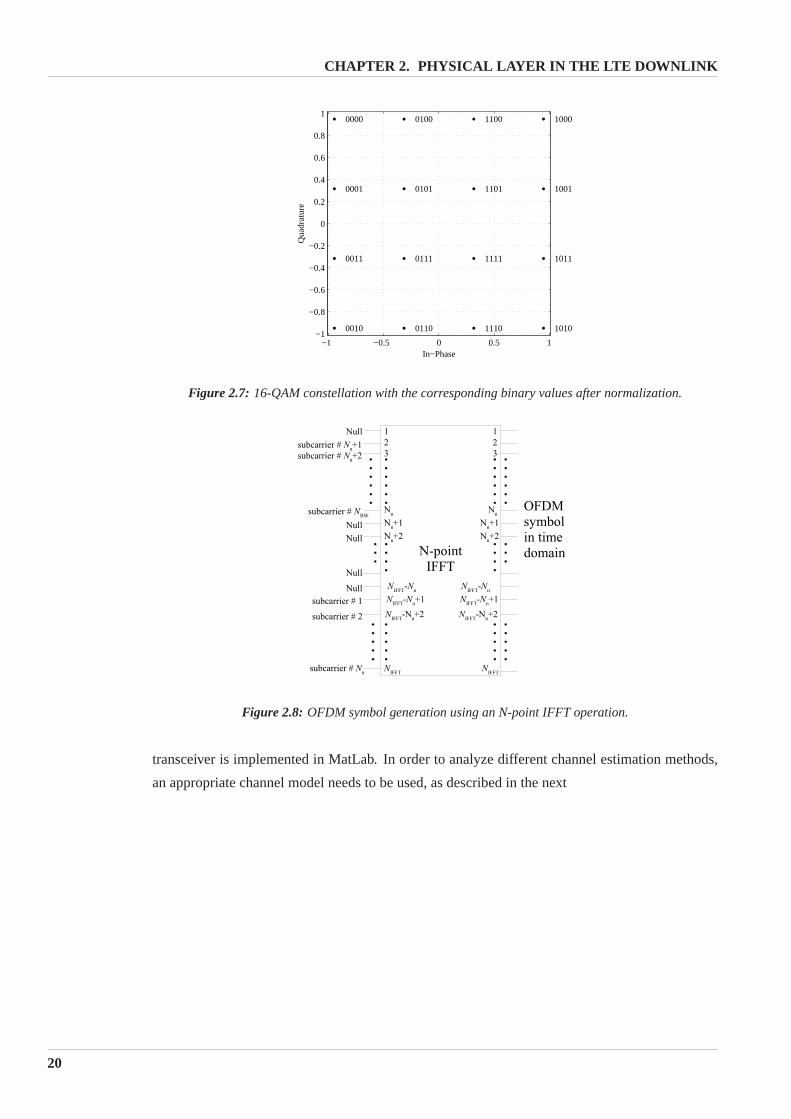
The bits are modulated using Gray labeling, which is depicted in Figure 2.7 for 16-QAM as an
Modulation Knorm
4-QAM 1√2
16-QAM 1√10
64-QAM 1√64
Table 2.2: Normalization factor for M-QAM modulation schemes in E-UTRA downlink [5].
example.
2.6.3 Inverse Fast Fourier Transform
Figure 2.8 shows an illustration of the mapping of symbols under IFFT-operation, which corre-
sponds to the mapping described in section 2.3.1.
2.7 Summary
Important properties of the physical layer in the LTE downlink have been described. For the
purpose of channel estimation, one antenna at transmitter side and receiver side is considered. The
channel estimation can be achieved separately for each antenna since thereference symbols are
orthogonal in space. OFDMA is utilized as multiple access scheme in the downlink, where each
user is allocated one or several resource blocks and scheduling is performed for each subframe.
Based on specifications in Release 7 [4] and on working assumptions in Release 8 [5] an OFDM
19
CHAPTER 2. PHYSICAL LAYER IN THE LTE DOWNLINK
−1 −0.5 0 0.5 1−1
−0.8
−0.6
−0.4
−0.2
0
0.2
0.4
0.6
0.8
1
Qua
drat
ure
In−Phase
0000
0001
0010
0011
0100
0101
0110
0111
1000
1001
1010
1011
1100
1101
1110
1111
Figure 2.7: 16-QAM constellation with the corresponding binary valuesafter normalization.
Figure 2.8: OFDM symbol generation using an N-point IFFT operation.
transceiver is implemented in MatLab. In order to analyze different channel estimation methods,
an appropriate channel model needs to be used, as described in the next
20

Channel Model 3
3.1 Multipath transmission
Radio wave propagation can be described by multiple paths occurring due toreflection (buildings,
trees, etc.) in the environment. When modeling a radio channel, only a finite number of paths is
considered to approximate the real environment, which is illustrated by Figure3.1. The received
Figure 3.1: Multipath radio environment [28, p. 7].
signal at the UE is a superposition of all paths. There are infinite number ofpaths closely spaced
in time, but only a finite number is modeled. Equation (3.1) describes a model for the channel
impulse response,
h′(τ) =K−1∑
k=0
αkδ(τ − τk), where (3.1)
K is the number of paths,αk is the complex fading coefficient for a given path at delayτk. In this
thesis a baseband representation of the channel is used, hence the effect of up-converting/transmit
filter and down-converting/receive filter is modeled byhT (τ) andhR(τ) respectively [28].
h(τ) = hT (τ) ∗ h′(τ) ∗ hR(τ), (3.2)

CHAPTER 3. CHANNEL MODEL
where∗ denotes convolution.
Applying the sampling operation at rate1/TC equation (3.2) is transformed into
h [k] = h [kTc] , where (3.3)
where the discrete time indexk ∈ {0, ..., L− 1} andL denotes the length of the sampled impulse
response. One channel model is the wide-sense stationary uncorrelated scattering (WSSUS). In
WSSUS model, the time-varying fading process is assumed to be wide-sense stationary random
process and the signal reflections from the scatterings by different objects are assumed to be inde-
pendent. The following parameters are often used to characterize a WSSUS channel:
- In order to describe the average delay of the channel the term delay spread,τRMS is used.
- Coherence bandwidth∆f(c) gives an indication of how far apart, in frequency, the signal
has to be spaced to in order to achieve correlation of valuec.
- Coherence time∆t(c) gives a measure of the time duration over which the correlation be-
tween two channel impulse response has a valuec. The coherence time is related to the
Doppler spectrum which depends on the velocity of the UE.
- Doppler spreadfDmax which indicates a maximum range of Doppler shifts.
The mentioned parameters are now described in detail and calculated for thesignal structure of
the physical layer in the LTE downlink. Furthermore standard channel models will be described
in order to find a suitable model for simulation purposes.
3.2 Delay Spread
The impact of the environment on the transmitted signal (fading) can also be classified as follows:
- Long-term fading: the fading varies slowly compared to the symbol time, it is not of interest
when estimating a channel. Typically it is caused by reflections from the geographical
surroundings, e.g. landscape.
- Short-term fading: Short-term fading can vary as fast as the symbol time. Short-term fading
is caused by the interference of multiple reflections, scattering and diffractions on small
elements in near surroundings., e.g. trees and other obstacles in the near.
The channel delay spreadτ is closely related to the short-term fading. In order to describe the
average delay of the channel, the root-mean-square (RMS) average of the delay spread, which is
defined as the second central moment of the channel power delay profile, is used [11, p. 540].
τRMS =
√∑K−1k=0 Pk(τk − τm)2∑K−1
k=0 Pk
, where (3.4)
τm =
∑K−1k=0 Pkτk∑K−1k=0 Pk
is the mean excess delay (3.5)
22

3.2. DELAY SPREAD
andPk is the power ofh[k] at time indexk. When the channel is viewed in frequency domain the
coherence bandwidth is of concern. Using the uncertainty relationship found in [9] the coherence
bandwidth is calculated as
∆f(c) ≥1
2πτRMSarccos(c), (3.6)
where∆f(c) is the minimal coherence bandwidth in which the autocorrelation of the channel
power delay profile,Rhh has the valuec.
A multipath channel is characterized as frequency flat or frequency selective in the following way:
Frequency flat fading: Coherence bandwidth∆fc >> Bs Symbol bandwidth . The frequency
components of the signal would roughly undergo the same fading.
Frequency selective fading:∆fc ≤ Bs, with c = 0.5 is in both cases. The different frequency
components of the signal, which differ by more than∆fc will undergo different degrees of fading.
In order to avoid ISI the delay spreadτRMS should always be less than symbol durationTs, such
that frequency flat fading is achieved. The data rate however will be decreased if the symbol
duration is extended.
3.2.1 Position of Reference Symbols in the Frequency Domain
The position of the reference symbols in frequency domain is investigated. Section 2.4.2 describes
the positions in detail. The goal is to compare the spacing between the reference symbols with the
coherence bandwidth of the channel.
3.2.2 Coherence Bandwidth
The spacing in frequency between the subcarriers is known from Section 2.3,
fspace= 15 kHz. (3.7)
According to Section 2.4.2 the reference symbols are placed at every 6th subcarrier:
fR = fspace· 6 = 90kHz. (3.8)
Using the uncertainty relationship described in Section 3.2 the bandwidthB(c) in which the chan-
nel is constant is defined forc = 0.9 and the valuec = 0.5 for when the channel has changed.
Based on these assumptions the coherence bandwidths are now calculated:
B(0.5) ≥ 1
2πτRMSarccos(c) =
1
2π0.65µsarccos(0.5) = 256.4kHz (3.9)
B(0.9) ≥ 1
2π0.65µsarccos(0.9) = 110.4kHz (3.10)
Equations (3.9) and (3.10) show that the spacing of the reference symbols in frequency approxi-
mately corresponds to the bandwidth in which the channel is constant, furthermore the channel is
estimated at least twice before the autocorrelation has the value 0.5.
23

CHAPTER 3. CHANNEL MODEL
3.3 Time-Varying channel
The mobile movement introduces Doppler frequency shifts. There are multipleDoppler shifts,
which add up and form a Doppler spectrum. In the following we consider one path.
3.3.1 Doppler shift
The main factor that affects the rate of fading is the mobility of the receiver relative to the trans-
mitter. As a UE moves with velocityvUE relative to NodeB, it causes a Doppler shiftfd which is
given by (3.11) for a singe path:
fd = fDmaxcos(θ), (3.11)
whereθ is the angle of arrival of the received signal relative to the direction of the UE and
fDmax =vUE
c0fc, (3.12)
wherefDmax is the maximum Doppler frequency ,vUE is the velocity of the receiver,fc is the
carrier frequency andc0 speed of light.
The time varying impulse response of the channel can be expressed as anextension of Equation
(3.1).
h(t, τ) =L−1∑
k=0
αkej2πfdtδ(τ − τk), (3.13)
wheret is the time at which the channel impulse response is measured. The signalh(t, τ) has a
band-limited spectrum, also denoted as Doppler spectrum. The spectrum is limitedto the range
W = [−νDmax, . . . , νDmax] , where (3.14)
νDmax = fDmaxTs, (3.15)
with Ts as the symbol duration andνDmax as the normalized maximum Doppler-shift. In mobile
radio channels, the maximum Doppler spread is used to characterize how fast in time the channel
changes. For this purpose the coherence time is calculated as [9]
∆t(c) ≥1
2πfDmaxarccos(c), (3.16)
where∆t(c) is the difference in time for which the autocorrelation in the time-domain has the
valuec.
A channel is said to be time-invariant, in the sense that the channel appearsas time invariant to the
transmitted signal.
Hence the terms are relative to the symbol duration: time selective fading occurs when the channel
changes within one symbol periodTs while time-invariant fading occurs when the channel is
constant within at least one symbol period.
24

3.4. TIME-FREQUENCY CORRELATION
Time-invariant fading:∆t(0.5) >> Ts, wherec = 0.5. If the symbol duration is small compared
with ∆t0.5 then the channel is classified as time-invariant.
Time selective fading:∆t(0.5) ≤ Ts. On the other hand if∆t(c) is close to or smaller than the
symbol duration , the channel is considered to have time selective fading. In general, it is difficult
to estimate the channel parameters for a time selective channel.
In order to estimate a channel for a period ofTs it is of importance to be in the time-invariant case.
3.3.2 Position of Reference Symbols in Time-Domain
The duration of one slotTslot is known from Section 2.3. There areNsym = 6 OFDM symbols in
one slot, which results in a symbol duration
Ts =Tslot
Nsym=
0.5 ms6
= 83.3 µs. (3.17)
Reference symbols are placed at each fourth OFDM symbol, but are notalways found at same
subcarriers. Nevertheless the channel can be estimated after each thirdOFDM symbol and hence
the spacing of reference symbols in the time-domain is set to,
TR = 3Ts = 0.250 ms (3.18)
Using the uncertainty relationship described in Section 3.2 the coherence bandwidth ∆f(c) in
which the channel is constant is defined forc = 0.9 and the valuec = 0.5 for when the channel
has changed.
A UE with a maximum speed of 120 km/h, has a maximum Doppler shift of 185.4 Hz. Based on
these assumptions the coherence times are now calculated
∆t(0.5) ≥ 1
2πfd, maxarccos(c) =
1
2π185.4Hzarccos(0.5) = 0.750 ms (3.19)
∆t(0.9) ≥ 1
2π222.15Hzarccos(0.9) = 0.323 ms (3.20)
Equations (3.19) and (3.20) show that the spacing of the reference symbols in time is less than the
coherence time . Furthermore the channel is estimated at least three times before the autocorrela-
tion of the channel estimates has the value 0.5.
3.4 Time-Frequency Correlation
For channel estimation purposes the channel correlation properties areof importance. Following
properties of the channel can be shown from [13, p. 93]:
R (∆t, ∆f) = R (∆t) R (∆f) (3.21)
Equation (3.21) is the autocorrelation of the time-varying channel frequency response, which is the
Fourier transform of (3.13) in the delay domain. The difference in time is denoted as∆t, while∆f
25

CHAPTER 3. CHANNEL MODEL
is the difference in frequency. Equation (3.21) is based on the fact thatin mobile radio channels the
time-correlation function is independent from the frequency correlation function [13]. Moreover
different assumptions can be made for these correlation functions. The frequency correlation
function is the Fourier transform of the power delay profile of the channel, hence it is based on
the power delay profile. The time-correlation depends on the Doppler power spectral density. The
Doppler power spectral density can be assumed uniform or having Jake’s spectrum [7]. In this
thesis the uniform spectral density is used. The constant spectrum can be expressed as,
Sh(ν,W) =
{1
2νDmax, ν ∈ W
0 otherwise,(3.22)
whereνDmax is defined in equation (3.15) withν asνDmax = fdTs andW in (3.14). The discrete
correlation function withRd(k) = R(kTs), based on [27], is then expressed as,
Rd (k,W) =1
j2πk|W|(ej2πkνDmax − e−j2πkνDmax
)
=sin(2πkνDmax)
πk|W| (3.23)
3.5 Standard Channel Models
Several models exist and are used in the industry to simulate radio wave propagation. Each model
is suitable for a certain type of environment. The channel model used in this project is based on
recommendations from 3GPP. The recommended channel models are chosen as simplifications, or
typical realizations of the COST 259 model [3]. Testing with a common channelmodel is imper-
ative to facilitate comparisons. The 3GPP typical urban (TU) channel model has been designed to
simulate high delay spread in urban environments using bandwidths up to 5 Mhz.
A simplified model for the power delay profile is given in (3.24) [26]. The tappowers are normal-
ized so that the sum of all tap powers is equal to 1.
Pk = η2[k] =e− k
LD
∑L−1k′=0 e
− k′
LD
, where (3.24)
LD =τRMS
TC(3.25)
denotes the RMS delay spreadτRMS normalized to the sampling rate1/TC andη is the amplitude
of the fading coefficient.
Assuming perfect power control and neglecting pathloss results in
L−1∑
k=0
η2[k] = 1 (3.26)
The supported lengthL of the sampled impulse response should be chosen with respect to the
signal-to-noise ratio (SNR) (Esσ2z
), at which the system is operating [28, p.8],
L ≥ 1 +τRMS
TCln (SNR) (3.27)
26
3.6. RAYLEIGH FADING CHANNELS
Hence the components of the impulse response smaller than the SNR are not taken into account.
Generation of a channel impulse response when the power delay profile isknown is achieved
assuming Rayleigh fading, which is described in next section.
3.6 Rayleigh Fading Channels
When a signal is transmitted in an environment with obstacles resulting in non line-of-sight
(NLOS) propagation, more than one transmission path will appear as a result of the reflections.
The receiver will then have to process a signal which is a superposition of several main transmis-
sion paths.
Each of the main paths is in reality the result of multiple scattered waves, or subpaths. If there
exists a large number of subpaths they may be modeled as statistically independent; the central
limit theorem will give the channel the statistical characteristics of a Rayleigh distribution [11, pp.
542-543].
The real and imaginary parts of the fading coefficient of one main pathα are independent and
identically Gaussian distributed with zero mean and varianceσ2
2 , which leads to the probability
density function
p(η) =η
σ2e−
η2
2σ2 , η ≥ 0 (3.28)
p(φ) =1
2π, −π ≤ φ ≤ π (3.29)
wherep(η) is the Rayleigh distribution,η is the amplitude of the fading coefficient and the phase
φ uniformly distributed.
Each tap is hence modeled as Gaussian real and imaginary part with zero mean with a variance
according to the power delay profile. The goal is to model the time variation of the channel
properties too. One method to simulate this phenomenon is to use Jake’s model [7]. However a
model developed by 3GPP, the Spatial Channel Model (SCM), described in the following Section
3.6.1, is used in this thesis in order to get as close to a true time varying channelas possible.
3.6.1 Spatial Channel Model
3GPP has developed a Spatial Channel Model (SCM) [2] for multiple inputmultiple output
(MIMO) systems in order to specify parameters intended for the three most common cellular
environments: suburban macrocells, urban macrocells, and urban microcells.
Since the goal of this project is channel estimation, pathloss is neglected.
The overall difference between the models are the amount and size of the scatterers. The macrocell
environments assume height of NodeB well above the height of scatterers, while the scatterers and
BS are at same height for the microcell scenario. From a UE’s point of view the delay spread is
one of the main parameters affected by the change in channel model as shown in Table 3.1. SCM
has been implemented in Matlab [21] and can be used to generate channel fading coefficients,
depending on several parameters such as the speed of UE, number of antennas and their properties
27

CHAPTER 3. CHANNEL MODEL
Channel Model Delay spread /τRMS
Urban micro cell 0.251µs
Urban macro cell 0.65µs
Suburban macro cell 0.17µs
Table 3.1: Root mean square delay spread for different channel models according to [2].
on transmitter and receiver side.
The SCM is designed for bandwidths up to 5 MHz, however support for bandwidths up to 20 MHz
is needed for modeling the LTE downlink, hence an extended version of SCM (SCME) has also
been developed [21].
This project makes use of the "Urban macro cell" channel model which specifies parameters for an
urban environment with up to 3 km distance to a base station and NLOS, since itis assumed that
the scatterers surrounding the UE are about the same height or are higher. This implies that the re-
ceived signal at the mobile antenna arrives from all directions after bouncing from the surrounding
scatterers, but there is no line-of-sight (LOS) to the NodeB.
3.7 Implementation of the Channel Model
The channel model is implemented with the OFDM transceiver as depicted in Figure 3.2. The
Figure 3.2: Block diagram of implementation of the SCME channel model with the transmitter and receiver.
transmitted signal is affected by the multipath channel generated by SCME andadditive white
Gaussian noise (AWGN) is added afterwards. In Section 3.3.2 it was concluded that the channel
was time-invariant within one OFDM symbol duration. Hence in this thesis the SCME channel
model is configured such that channel impulse responses are generated for each OFDM symbol
and convolved with the symbol.
28
3.7. IMPLEMENTATION OF THE CHANNEL MODEL
3.7.1 AWGN
Since the subcarriers of the transmitted signal are normalized, the signal-to-noise ratio is controlled
by adjusting the noise varianceσ2z . The average energy of one OFDM symbol is calculated as
following,
ES =NBW
NIFFT. (3.30)
The resulting SNR is calculated as
SNR =ES
EN=
NBW
NIFFT
1
σ2z
. (3.31)
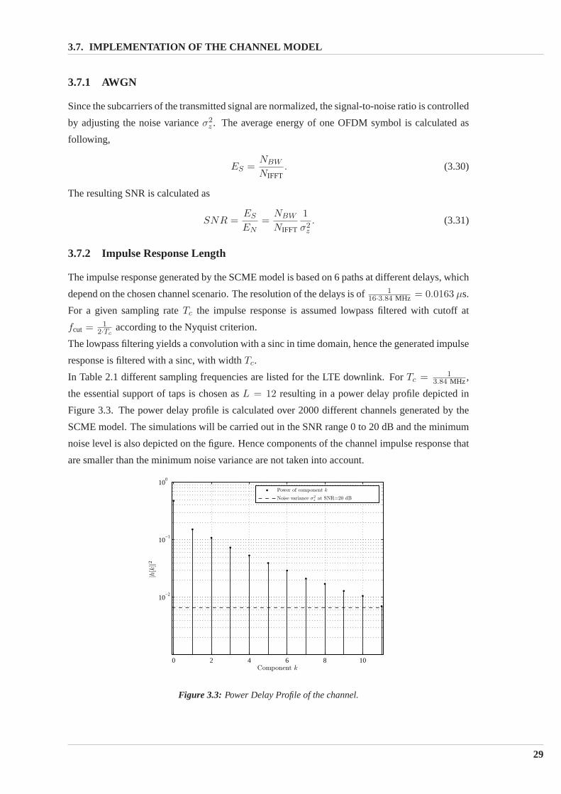
3.7.2 Impulse Response Length
The impulse response generated by the SCME model is based on 6 paths at different delays, which
depend on the chosen channel scenario. The resolution of the delays isof 116·3.84 MHz = 0.0163 µs.
For a given sampling rateTc the impulse response is assumed lowpass filtered with cutoff at
fcut =1
2·Tcaccording to the Nyquist criterion.
The lowpass filtering yields a convolution with a sinc in time domain, hence the generated impulse
response is filtered with a sinc, with widthTc.
In Table 2.1 different sampling frequencies are listed for the LTE downlink. For Tc = 13.84 MHz ,
the essential support of taps is chosen asL = 12 resulting in a power delay profile depicted in
Figure 3.3. The power delay profile is calculated over 2000 different channels generated by the
SCME model. The simulations will be carried out in the SNR range 0 to 20 dB and the minimum
noise level is also depicted on the figure. Hence components of the channel impulse response that
are smaller than the minimum noise variance are not taken into account.
0 2 4 6 8 10
10−2
10−1
100
Component k
|h[k
]|2
Power of component k
Noise variance σ2
zat SNR=20 dB
Figure 3.3: Power Delay Profile of the channel.
29

CHAPTER 3. CHANNEL MODEL
3.8 Summary
In order to do simulations as close to the reality as possible, it is important to have agood channel
model. Mobile channel models with time invariant and time variant behavior have been investi-
gated. The chosen channel model is the SCME (Spatial Channel Model Extended), which gen-
erates channel coefficients based on the 3GPP channel model specifications. The channel model
supports a typical urban area scenario as well as mobility of the UE. Moreover the selection of
the impulse response length and adapting the impulse response to a sampling frequencyTc has
been described in order perform simulation of channel estimation methods withthe LTE downlink
structure.
30
Time-Invariant Channel Esti-
mation4
This chapter describes different channel estimation techniques to be used for the time-invariant
downlink case.
By focusing on time-invariant channels, only the frequency-domain needs to be considered. Hence
three different channel estimators are applied in the frequency-domain and compared. Since the
estimation is aimed for the UE, the complexity should be minimized.
4.1 OFDM Signal Model
In Appendix A.7 the OFDM signal model is presented. As stated in (A.29), thesignal model for
OFDM transmission can be expressed as
y[m] = diag(g)d[m] + z[m]. (4.1)
In order to ease the calculation of the channel estimation, the signal model is simplified in the
following section.
4.1.1 Signal Model Simplification
The channel is estimated for each OFDM symbol and the general focus ofthe channel estimation
will be on only one OFDM symbol. For the sake of simplicity the indexm is dropped and equation
(4.1) is rewritten as
y = XFh + z, (4.2)
wherey ∈ CNIFFT is the received OFDM symbol,X ∈ C
NIFFT,NIFFT is a diagonal matrix with data,
reference symbols or zeros whileh ∈ CNIFFT is the channel impulse response andz ∈ C
NIFFT is
the noise which is assumed to be white Gaussian.F ∈ CNIFFT×NIFFT is the same DFT-matrix as
described in (A.13),
F =
f1,1 . . . f1,NIFFT
.... . .
...
fNIFFT,1 . . . fNIFFT,NIFFT
. (4.3)

CHAPTER 4. TIME-INVARIANT CHANNEL ESTIMATION
The channel estimation will be based on transmitted reference symbols, whichare scattered as
described in Section 2.4.2, i.e. an interpolation has to be performed in order toobtain the channel
estimates for the subcarriers with data symbols. Before the first estimation method is introduced,
prior knowledge about the channel is used to reduce the complexity of the estimator.
Based on the knowledge of the channel model and of the reference symbols two following as-
sumptions can be made [24]:
- If the channelh has the maximum delay at tapL − 1, only the firstL columns ofF can be
considered, since the rest is multiplied by zero.h′ ∈ CL denotes the firstL coefficients of
h.
- The transmitted reference symbols are scattered (see Figure 2.4), hence only rows corre-
sponding to the position of these symbols need to be considered for the diagonal matrix
X.
Equation (4.2) is rewritten as
yr = XrTrh′ + zr, (4.4)
whereXr = diag(xr(1) . . . xr(Nr)) and
Tr =
ftr(1),1 . . . ftr(1),L
.... . .
...
ftr(Nr),1 . . . ftr(Nr),L
. (4.5)
Nr denotes the number of reference symbols for one OFDM symbol, whilexr(i) andtr(i) denote
the i’th reference symbol in the frequency-domain and the index of the subcarrier carring the
symbol respectively.zr ∈ CNr is the truncated noise and is still white Gaussian.
The channelh′ is estimated based on the knowledge of transmitted reference symbolsxr.
4.2 Least Squares Estimator
Knowing the the transmitted reference symbols, the first estimate to be calculatedis the least
squares estimator in the frequency-domain for the channel impulse response:
gLS =
[yr(1)
xr(1),
yr(2)
xr(2), · · · ,
yr(Nr)
xr(Nr)
], (4.6)
wheregLS ∈ CNr can only be estimated over the subcarriers carrying reference symbols.Hence
this result has to be interpolated over the full frequency range in order togive an estimate for
subcarriers with data symbols.
The interpolation can be performed in frequency domain or in time domain. For the latter case the
interpolation is carried out by only taking the firstL channel taps into account and setting all other
taps to zero. After estimating theL-tap channel, the channel is transformed back into frequency
domain. This approach is investigated by applying linear minimum mean square error (LMMSE)
estimator in Section 4.3 and least-squares (LS) estimator in Section 4.4.
32
4.3. LINEAR MINIMUM MEAN SQUARED ERROR ESTIMATOR
4.3 Linear Minimum Mean Squared Error Estimator
The LMMSE estimator, calculates the channel impulse response (CIR)h , that minimizes the
mean squared errorE{
h − h′}
, givenyr andXr [24].
h = RhyrR−1yryr
yr (4.7)
The autocorrelation matrices are calculated as follows:
Ryryr = E[yryr
H]
= XrTrE[hhH]XH
r TrH + E
[zrzr
H]+ XrTr[hzr
H]+[nrh
H]T Hr Xr
H
= XrTrRh′h′T Hr XH
r + σz2INr (4.8)
=1
LXrTrT
Hr XH
r + σz2INr (4.9)
In order to simplify calculations it is assumed that the channel coefficients are independent and
the energy for each tap is1/L, i.e. the power delay profile is uniformRh′h′ = E[h′h′H] = 1
LI.
Rh′yr = E[h′yr
H]
= E[h′h′HT H
r XHr + zrh
HT Hr XH
r
]
= Rh′h′T Hr XH
r (4.10)
=1
LT H
r XHr . (4.11)
Similar to (4.4), the transmission of data symbols can be described as
yd = XdTdh′ + zd, (4.12)
whereXd = diag(xd(1) . . . xd(Nd)) and
Td =
ftd(1),1 . . . ftd(1),L
.... . .
...
ftd(Nd),1 . . . ftd(Nd),L
. (4.13)
Nd denotes the number of data symbols for one OFDM symbol, whilexd(i) andtd(i) denote the
i’th data symbol and the index of the subband carring the symbol respectively. zd ∈ CNd is the
truncated Gaussian noise.
The calculated value forh′ is transformed into frequency domain for the subcarriers containing
data symbols,
g = Tdh ≈ Tdh′. (4.14)
The frequency response of the channel is now interpolated using LMMSE estimation with low
complexity and the estimate is passed to the equalizer. It should be noted that for the case with
the true autocorrelationRh′h′ and not uniform as assumed this method is equal to the Wiener
interpolation [14].
33

CHAPTER 4. TIME-INVARIANT CHANNEL ESTIMATION
4.4 Downsampling
Section 4.2 gives an estimate for the LS frequency response of the channel. Now a LS estimate
in the time domain is calculated. By modifying (4.2) it is transformed into the time domain. To
understand the idea behind this method, let us consider the received signal r in time for one OFDM
symbol.
r = F HXFLh′ + zt, (4.15)
whereh′ ∈ CL is theL-tap channel impulse response andFL ∈ C
NIFFT×L is the Fourier matrix
that gives the frequency domain representation overNIFFT subcarriers of the channel, whileX is
the transmitted symbols.
F H ∈ CNIFFT×NIFFT transforms the attenuated signal in frequency domain into time domain, where
r is the time domain representation ofy from (4.2) andzt is the complex Gaussian noise.
4.4.1 Least-Squares Estimation in Time
From (4.15) the received signalr is equivalent to
r = Sh′ + zt, (4.16)
where
S = F HXFL, (4.17)
and the diagonal matrixX containing the complex symbols modulated over the subcarriers can
be expressed as:
X = Ad + Ar, (4.18)
whereAd ∈ CNIFFT×NIFFT andAr ∈ C
NIFFT×NIFFT are diagonal matrices containing non-zero ele-
ments in the positions of the transmitted data and of the transmitted reference symbols respectively.
Since the transmitted symbols are unknown, an approximation of the matrixS is made such that
only transmitted reference symbols are taken into account:
S = F HArFL. (4.19)
The channel impulse response in least-squares sense is found as [6]
hLS =(SHS
)−1SHr. (4.20)
Inserting (4.19) into (4.20) yields,
hLS =(F H
L AHr ArFL
)−1F H
L AHr Fr =
(F H
L AHr ArFL
)−1F H
L AHr y (4.21)
From a computational point of view the LS estimator is simple since the matrix
(F H
L AHr ArFL
)−1F H
L AHr
34

4.4. DOWNSAMPLING
is constant. In the LTE application, the matrix inversion can be computed once and used regardless
of the varying channel statistics. This of course is based on the assumptionthat the positions
of the reference symbols do not change. However, an ill-conditioned problem caused by the
matrix inversion occurs in the implementation of the LS estimator. The problem can be solved by
regularizing the eigenvalues of the matrix to be inverted by adding a small constant term to the
diagonal [6] or by downsampling.
4.4.2 Downsampled impulse response LS channel estimation
The ill-conditioning problem stems from the structure of the subcarriers in theLTE downlink.
Only the center of the frequency spectrum is utilized, while the rest is set to zero.
As an example the case ofNIFFT = 2048 from Table 2.1 is considered. The number of occupied
subcarriers is only 1200. Hence, while the sampling frequency is 30.72 MHz (NIFFT · fspace),
the occupied bandwidth is only 18 MHz (NBW · fspace). In LTE the occupied bandwidth is ap-
proximately2/3 of the whole bandwidth. The goal is to get the occupied bandwidth close to the
sampling frequency which can be accomplished by downsampling to2/3 of the sampling fre-
quency. In practice, the channelh′ is not estimated in all theL taps but only in 2 out of 3 taps
hereby obtaining the average downsampling factor2/3, as described in (4.23).
gDS = FLh′ =
f1,1 f1,2 f1,3 . . . f1,L
f2,1 f1,2 f2,3 . . . f2,L
f3,1 f3,2 f3,3 . . . f3,L
f4,1 f4,2 f4,3 . . . f4,L
......
......
...
fN,1 fN,2 fN,3 . . . fN,L
h′0
h′1
0
h′3
h′4
0...
h′L
(4.22)
= F DShDS =
f1,1 f1,2 f1,4 . . . f1,L
f2,1 f1,2 f2,4 . . . f2,L
f3,1 f3,2 f3,4 . . . f3,L
f4,1 f4,2 f4,4 . . . f4,L
......
......
...
fN,1 fN,2 fN,4 . . . fN,L
h′0
h′1
h′3
h′4...
h′L−1
(4.23)
By removing each third column inFL resulting inF DS ∈ CNIFFT×LDS the calculations are simpli-
fied and the complexity is reduced.
Equation (4.15) is now written as
r = F HArFDShDS + zt, (4.24)
35

CHAPTER 4. TIME-INVARIANT CHANNEL ESTIMATION
and the least square channel impulse response can be calculated as
hDS =(F DS,HAr
HArFDS)−1
F DS,HArHy. (4.25)
The channel impulse responsehDS is transformed into frequency domain by multiplying with
F DS, such that
gDS = F DSd hDS = F DS
d
(F DS,HAr
HArFDS)−1
F DS,HArHy, (4.26)
whereF DSd is the truncated version ofF DS, only containing rows coresponding to positions of
the data symbols. Utilizing knowledge of the transmitted reference symbols the complexity of
equations (4.25) and (4.26) can be reduced even further.
4.4.3 Further explanation on downsampling
In [6] the downsampling to2/3 of the sampling frequency is performed by estimatingh′ only in
2 out of 3 taps.
In order to explain the purpose of this step, the downsampling procedure isinvestigated. Figure 4.1
shows an equivalent representation the downsampling of the non-integerfactor2/3 is performed
[17]. h′ is upsampled by a factor of two as follows,
Figure 4.1: System for changing the sampling rate by a non-integer factor [17].
ho = [h[0], 0, h[1], 0, h[2], 0, h[3], 0, . . . , h[L − 1], 0] . (4.27)
The frequency response of the upsampled impulse response is illustrated on Figure 4.2(b). The
frequency response of the channel is only illustrated as rectangular asan example. The one-sided
bandwidth of the channel is assumed to be at most2/3 of half the sampling frequency,
fBW =2
3f ′
s, (4.28)
wheref ′s = fs
2 .
After 2x upsampling to sampling frequencyfo = 2fs the maximum one sided bandwidth of the
channel is now at most1/3 of half the new sampling frequency,
f ′BW =
1
3f ′
o. (4.29)
36

4.4. DOWNSAMPLING
wheref ′o = fo
2 .
In order to avoid aliasing when downsampling with factor three, a lowpass filter is introduced as
in Figure 4.2(c). The method proposed in [6] is equivalent to the following lowpass filter:
hlp = [1, 1] , (4.30)
resulting in a filtered impulse response,
ho = [h[0], h[0], h[1], h[1], h[2], h[2], h[3], h[3], . . . , h[L − 1], h[L − 1]] . (4.31)
Ideally the lowpass filter should have cutoff at1/3f ′o [17] but usinghlp results in a sinc-function
in frequency domain with an one-sided bandwidth off ′o which is depicted in Figure 4.2(c). The
(a) Frequency response of the sampledh.
(b) Frequency response of the over sampledho.
(c) Frequency response of the lowpass filterhlp andho.
(d) Frequency response of the downsampled impulse response
hDS with aliasing which is the dottet line.
downsampling of factor three is achieved by taking each third sample ofho,
hDS =
[h[0]↑
, h[0], h[1], h[1]↑
, h[2], h[2], h[3]↑
, h[3], . . . , h[L − 1]↑
, h[L − 1]
]
= [h[0], h[1], h[3], h[4], . . . , h[L − 1]] (4.32)
where it is assumed thath[L− 1] is also an element to be selected in the downsampling. Equation
(4.32) is exactly the result described in Section 4.4.2 equation (4.23). The downsampled sampled
37

CHAPTER 4. TIME-INVARIANT CHANNEL ESTIMATION
frequency can be written asfDS = 1/3fo = 2/3fo. The frequency response of the downsampled
impulse response is depicted on Figure 4.2(d), where the presence of aliasing is illustrated with
the dotted line.
4.4.4 Complexity Reduction
From the structure of the reference signals described in Section 2.4.2 it is known that the norm is
1. Hence the termArHAr in (4.25) consists of ones at reference positions and zeros otherwise.
The matrix inversion is rewritten according to this observation,
(F DS,HAr
HArFDS)−1
F DS,H =(Fr
DS,HF DSr
)−1Fr
DS,H, (4.33)
whereF DSr is the truncated version ofF DS
L only containing rows corresponding to reference sym-
bol positions. Equation (4.26) with reduced complexity is now expressed as
gDSd = F DS
d hDS = F DSd
(Fr
DS,HF DSr
)−1Fr
DS,HXrHyr, (4.34)
with XHr andyr only containing values corresponding to reference positions as described in Sec-
tion 4.1.1.
4.5 Reduced Rank LMMSE
Least Squares and LMMSE channel estimation in time-domain have been presented so far. Now
LMMSE estimation in frequency-domain using rank reduction is investigated.
Rank reduction is achieved by using the singular value decomposition (SVD)in the calculation of
the LMMSE of the channel frequency response. The LMMSE estimator in frequency domain is
found by [8]:
gLMMSE = RggLSR−1gLSgLS
gLS, (4.35)
wheregLS ∈ CNr is the least square channel frequency response, estimated using transmitted
reference symbols as in (4.6). To be able to calculate the autocorrelationRggLSbetween the full
range,g ∈ CNIFFT, and least squares frequency response, the vectorgLS is set as a function ofg
by the following steps:
yr = XrTr1√
NIFFTFL
Hg + zr (4.36)
g is transformed into time domain by a DFT-matrixFL ∈ CIFFT,L, whereL is the number of
channel taps andN is the DFT-size. The frequencies corresponding to the subcarriers of the
reference symbols are then extracted byTr and multiplied with the transmitted reference symbols.
gLS can now be expressed as
gLS = Tr1√
NIFFTFL
Hg + Xr−1zr. (4.37)
38
4.6. LINEAR INTERPOLATION
Finally RggLS is estimated using
RggLS = E[ggLS
H] (4.38)
= E
[g
(gH 1√
NIFFTFLTr
H + zrHX−1,H
)]
=1√
NIFFTFLTr
H (4.39)
As in (4.9) each tap in the channel impulse response is assumed to have energy 1L , hence
E[ggH] = FLRh′h′F H
L =1
LFLF H
L . (4.40)
The same approach is used to calculateRgLSgLS.
RgLSgLS = E[gLSgLS
H] (4.41)
= E
[Tr
1√NIFFT
FLHggH 1√
NIFFTFLTr
H + Xr−1zrzr
HXr−1,H
]
=1
NIFFTTrFL
HFLTrH + E
[σz
2(XrXr
H)−1]
=L
NIFFTTrTr
H + σz2I, (4.42)
whereF HL FL = LIL.
The average energy of the transmitted symbols are normalized to one, henceE[XrXr
H]
= IL.
In order to reduce the rank of the LMMSE estimate, (4.35) is factorized into [8],
gLMMSE = RggLSR−0.5gLSgLS
R−0.5gLSgLS
gLS. (4.43)
The SVD is performed on the first two factors
RggLSR−0.5
gLSgLS= Q1DQ2
H. (4.44)
The best rank-p estimator is then
gp = Q1
[Dp 0
0 0
]Q2
HR−0.5gLSgLS
gLS
= Q1D′Q2
HR−0.5gLSgLS
gLS (4.45)
whereDp is the upperp × p left corner ofD, i.e. only the singular vectors associated to the
p largest singular values are kept and the rest is set to zero. Hereby noise can be reduced by
neglecting subspaces with low energy. The rankp is set as the estimated number of channel taps
(p = L) [8]. It is also possible to further simplify (4.45) according to [18] in order to reduce the
complexity. Equation (4.45) however is implemented in Matlab in order to compare this method
with others.
4.6 Linear Interpolation
A simple way of performing interpolation is the to use linear interpolation. This is possible since
the spacing between the reference symbols corresponds to the coherence bandwidth of the channel
as described in Section 3.2.1.
39

CHAPTER 4. TIME-INVARIANT CHANNEL ESTIMATION
4.7 Complexity of the Considered Estimators
The complexity of the frequency response estimation depends on the chosen method. The com-
plexity is given in the formO(N) in order to give an overview of the calculations. Table 4.7 lists
the calculations and their complexity based on [10]. It should be noted that the listed complexity
is for one OFDM symbol withNr as the total number of estimates. From Table 4.7 it is clear
that the reduced rank LMMSE estimator is the most complex because of the SVDcalculation
and matrix inversion. The LMMSE CIR requires one matrix inversion, while thecalculation of
downsampled CIR is only a matrix multiplication. The simplest method is the linear interpolation,
which requires a constant number of floating point operations as a function of (Nr − 1). For a
fixed signal to noise ratio however we can precompute most of the calculationand hereby reduce
the calculation complexity. In this case the LMMSE CIR estimator requires step 3 and 4, while
the reduced rank LMMSE estimator requires step 5. This yields a low-complexity approach from
a calculation point of view to estimate the channel frequency response.
4.8 Summary
Estimation methods for calculation of the frequency response have been presented for the LTE
downlink in the time-invariant channel. The performed estimation is based on transmitted refer-
ence symbols. The presented algorithms are LMMSE CIR estimator, downsampled CIR estimator,
reduced rank LMMSE estimator and linear interpolation. The LMMSE CIR anddownsampled
CIR present a way to estimate the channel impulse response based on assumptions of the number
of tapsL. The downsampled CIR furthermore makes use of the fact that the LTE downlink only
occupies2/3 of the transmitted bandwidth. The complexity of the algorithms have been reviewed
and it is shown that the reduced rank LMMSE has the highest complexity, followed by LMMSE
CIR and downsampled CIR. It is also shown that with a fixed SNR we can reduce the calculation
complexity for the LMMSE CIR estimator and the reduced rank LMMSE estimator.The mobile
channel is not time-invariant hence a method has to be found in order to alsoperform estimation
in a time-varying channel. The next chapter introduces a method to cope with such channels.
40
4.8. SUMMARY
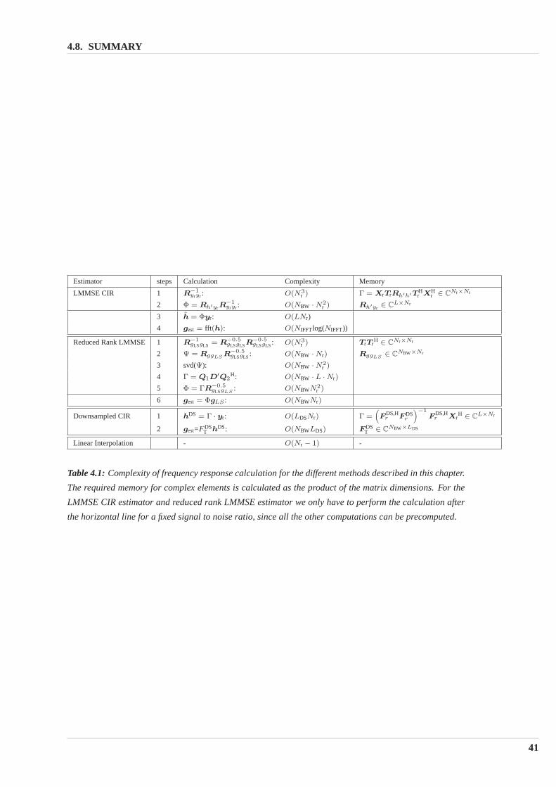
Estimator steps Calculation Complexity Memory
LMMSE CIR 1 R−1yryr : O(N3
r ) Γ = XrTrRh′h′THr XH
r ∈ CNr×Nr
2 Φ = Rh′yrR−1yryr : O(NBW · N2
r ) Rh′yr ∈ CL×Nr
3 h = Φyr: O(LNr)
4 gest = fft(h): O(NIFFTlog(NIFFT))
Reduced Rank LMMSE 1 R−1gLSgLS = R−0.5
gLSgLSR−0.5gLSgLS : O(N3
r ) TrTrH ∈ CNr×Nr
2 Ψ = RggLSR−0.5
gLSgLS : O(NBW · Nr) RggLS∈ CNBW×Nr
3 svd(Ψ): O(NBW · N2r )
4 Γ = Q1D′Q2H: O(NBW · L · Nr)
5 Φ = ΓR−0.5gLSgLS
: O(NBWN2r )
6 gest = ΦgLS : O(NBWNr)
Downsampled CIR 1 hDS = Γ · yr: O(LDSNr) Γ =(FDS,H
r FDSr
)−1
FDS,Hr Xr
H ∈ CL×Nr
2 gest=F DST hDS: O(NBWLDS) FDS
T ∈ CNBW×LDS
Linear Interpolation - O(Nr − 1) -
Table 4.1: Complexity of frequency response calculation for the different methods described in this chapter.
The required memory for complex elements is calculated as the product of the matrix dimensions. For the
LMMSE CIR estimator and reduced rank LMMSE estimator we onlyhave to perform the calculation after
the horizontal line for a fixed signal to noise ratio, since all the other computations can be precomputed.
41

CHAPTER 4. TIME-INVARIANT CHANNEL ESTIMATION
42

Time-Varying Channel Estima-
tion5
The mobility of the UE and the surrounding objects leads to a time-varying channel which needs
to be tracked. As described in Section 3.3.1 this results in a Doppler shift. In order to estimate the
time-varying channel, the discrete prolate spheroidal (DPS) basis expansion is utilized. Firstly, the
general idea behind time-varying channel estimation is introduced before describing the utilization
of the DPS basis expansion in detail.
5.1 Initial Steps in the Time-Varying Channel Estimation
The goal of channel estimation is to estimate the time-varying channel frequency response for each
OFDM symbol. In Section 3.3.2 it is concluded that the channel is constant within the duration of
one OFDM symbol. In Chapter 4 it was investigated how to estimate the channel using scattered
reference symbols in the frequency domain. Since the reference symbolsare also scattered in the
time-domain, it is necessary to estimate the channel in two dimensions, in the time-domain as well
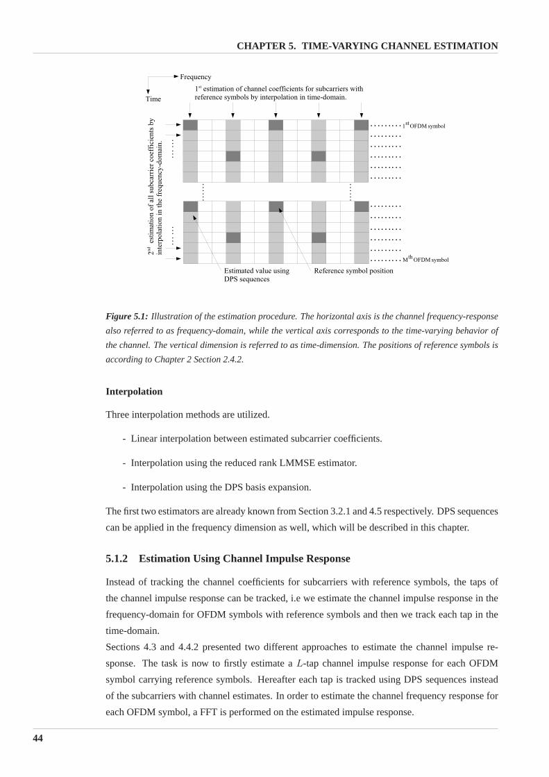
as in the frequency-domain. The principle of the estimation procedure is shown in Figure 5.1. The
channel can also be represented by its impulse response instead of its frequency response and the
time-varying behavior of the impulse response can be tracked. The methodsto be used for these
two different ways of tracking the channel are presented in the next sections.
5.1.1 Estimation of Subcarrier Coefficients
In order to track the channel frequency response, the subcarrierswith reference symbols are used
to find estimates of the channel for the subcarriers at OFDM symbols withoutreference symbols.
This can be illustrated by Figure 5.1. Firstly, the channel is estimated in the time direction of all
subcarriers with reference symbols using DPS sequences. This method allows a channel estimate
to be found for each third subcarrier at each OFDM symbol. Secondly, the frequency response
for each OFDM symbol is found by interpolating in the frequency-domain between the known
estimates. Let us denote the number of reference symbols for subcarriers and OFDM symbols
carrying them asNr andMr respectively. The notationM is used in order to emphasize that the
reference symbols in time-domain are considered.
CHAPTER 5. TIME-VARYING CHANNEL ESTIMATION
Figure 5.1: Illustration of the estimation procedure. The horizontal axis is the channel frequency-response
also referred to as frequency-domain, while the vertical axis corresponds to the time-varying behavior of
the channel. The vertical dimension is referred to as time-dimension. The positions of reference symbols is
according to Chapter 2 Section 2.4.2.
Interpolation
Three interpolation methods are utilized.
- Linear interpolation between estimated subcarrier coefficients.
- Interpolation using the reduced rank LMMSE estimator.
- Interpolation using the DPS basis expansion.
The first two estimators are already known from Section 3.2.1 and 4.5 respectively. DPS sequences
can be applied in the frequency dimension as well, which will be described in this chapter.
5.1.2 Estimation Using Channel Impulse Response
Instead of tracking the channel coefficients for subcarriers with reference symbols, the taps of
the channel impulse response can be tracked, i.e we estimate the channel impulse response in the
frequency-domain for OFDM symbols with reference symbols and then we track each tap in the
time-domain.
Sections 4.3 and 4.4.2 presented two different approaches to estimate the channel impulse re-
sponse. The task is now to firstly estimate aL-tap channel impulse response for each OFDM
symbol carrying reference symbols. Hereafter each tap is tracked using DPS sequences instead
of the subcarriers with channel estimates. In order to estimate the channel frequency response for
each OFDM symbol, a FFT is performed on the estimated impulse response.
44

5.2. SLEPIAN BASIS EXPANSION
Common for all estimation methods is the use of DPS sequences, which will be explained in the
following section.
5.2 Slepian Basis Expansion
In order to estimate the time-varying channel at the UE, an efficient representation of the channel
is needed. The channel is estimated over a block ofM OFDM symbols with a Doppler spectrum
as defined in (3.22) with a maximum Doppler shift ofνDmax.
In order to model the time-varying channel, the effect of the Doppler shiftsneed to be modeled
accurately. One way of modeling it is to make use of basis expansion models. In this thesis a basis
expansion model based on DPS sequences will be utilized that is based on [28] and [26].
Slepian [22] investigated which sequencesu[m] are concentrated in a certain time interval of
lengthM [28, p. 52 ff.],
λ(νDmax, M) =
∑M−1m=0 |u[m]|2
∑∞−∞ |u[m]|2
, with 0 ≤ λ ≤ 1. (5.1)
and simultaneously band-limited in frequency to the intervalW = [−νDmax, . . . , νDmax]
u[m] =
∫ νDmax
−νDmax
U(ν)ej2πmνdν, where (5.2)
U(ν) =∞∑
−∞u[m]e−j2πmν . (5.3)
The solutions for the optimization problems (5.1) (5.2) and (5.3) are the discrete prolate spheroidal
sequences. The sequencesui[ℓ, νDmax, M ] are defined as the real solution of
M−1∑
ℓ=0
sin(2πνDmax(ℓ − m))
π(ℓ − m)ui[ℓ,W, M ] = λi(νDmax, M)ui[m,W, M ] (5.4)
for i ∈ {0, . . . , M − 1} = I andm ∈ Z. In the sequel a system with fixed parameters(W, M) is
considered and the dependency on these parameters is dropped.
The DPS sequenceui[m] is a unique sequence which is exactly band-limited and having a high
energy concentration within the time intervalM . The sequences are doubly orthonormal on the
infinite set{−∞, . . . ,∞} = Z as well as the finite set{0, . . . , M − 1},
M−1∑
m=0
ui[m]uj [m] = λi
∞∑
−∞ui[m]uj [m] = δij , (5.5)
wherei, j ∈ {0, . . . , M − 1}. The eigenvaluesλi of the sequencesui[m], expressed by (5.1)
have the following property [28, p. 53]:
- The values ofλi are clustered near 1 fori ≤ ⌈2νDmaxM⌉ + 1
45

CHAPTER 5. TIME-VARYING CHANNEL ESTIMATION
- For i > ⌈2νDmaxM⌉ + 1 they rapidly drop to zero.
Hence the dimension of the signal space [22] is approximately given by
D′ = ⌈2νDmaxM⌉ + 1 (5.6)
For the purpose of channel estimation, only the index setm ∈ {0, . . . , M − 1} is of concern and
these limited sequences are denoted as Slepian sequences. The vectorui ∈ RM is now defined
containing elementsui[m] for m ∈ {0, . . . , M − 1} and equation (5.4) is written as:
Cui = λiui, (5.7)
with matrixC defined as
[C]i,ℓ =sin(2πνDmax(i − ℓ))
π(i − ℓ), for i, ℓ ∈ {0, . . . , M − 1}, (5.8)
where[C]i,ℓ denotes the value ofC at rowi columnℓ.
The theory of time-concentrated and band-limited sequences developed bySlepian leads to a new
approach for the time-varying channel estimation. The Slepian sequencesspan an orthonormal
basis allowing a representation of time-limited snapshot of a band-limited signal using a minimum
number of basis functions. The Slepian sequences expand the sequenceg[m] as follows:
g[m] ≈ g[m] =D−1∑
i=0
ui[m]γi, (5.9)
whereγi is the weighting coefficients of the Slepian sequences andm ∈ {0, . . . , M − 1}. The
dimensionD has the constraints,
D′ ≤ D ≤ M. (5.10)
The choice ofD affects the mean square error (MSE) defined as,
MSEM =1
M
M−1∑
m=0
E
{|g[m] − g[m]|2
}. (5.11)
5.2.1 Estimation of Channel Parameters
In order to utilize a basis expansion for channel estimation, the received OFDM signal is investi-
gated. The received signaly[m, q] for OFDM symbol at time indexm for subcarrierq. For a fixed
subcarrier, the indexq is dropped resulting in
y[m] = g[m]d[m] + z[m], (5.12)
whereg[m] is the channel attenuation,d[m] the transmitted symbol andz[m] is white Gaussian
noise. Using a basis expansion (5.12) can be written as,
y[m] ≈(
D−1∑
i=0
ui[m]γi
)d[m] + z[m]. (5.13)
46
5.2. SLEPIAN BASIS EXPANSION
If d[m] has unit norm and is known for allm, an estimate of the channel coefficientg[m] is found
as
g[m] = y[m]d∗[m] = g[m] + z[m]d∗[m]. (5.14)
The weighting coefficientγi for i ∈ 0, . . . , D − 1 is calculated as,
γi =M−1∑
m=0
g[m]u∗i =
M−1∑
m=0
y[m]d∗[m]u∗i [m]. (5.15)
The estimated sequenceg[m] is finally written as,
g[m] = fT [m]γ =
(D−1∑
i=0
ui[m]γi
), (5.16)
where
f [m] =
ui[m]...
uD−1[m]
∈ RD (5.17)
and
γ =
γi
...
γD−1
∈ CD. (5.18)
It can be shown that the Slepian basis expansion is a reduced-rank channel estimation. The fol-
lowing section describes reduced-rank estimation in general.
5.2.2 Reduced-Rank Channel Estimation
Reduced-rank channel estimation is expressed in equation (5.9), which also can be written as [27],
g[m] ≈ g[m] =
D−1∑
i=0
ui[m]γi = U γ, where (5.19)
U = [u0, . . . ,uD−1] , with (5.20)
ui = [ui[0], ui[1], . . . , ui[M − 1]]T , i ∈ {0, . . . , D − 1} . (5.21)
An estimate of the basis expansion coefficientsγ is found the same way as in (5.15), but here
expressed in a matrix-vector notation, simplified as [27],
γ = UHg (5.22)
because of the orthonormality of the basis vectors. The reconstruction error per data block is
defined as [27],
z =1
M||g − g| |2 =
1
M
∥∥UHn∥∥2
+1
M
∣∣V Hg∣∣2 , (5.23)
47
CHAPTER 5. TIME-VARYING CHANNEL ESTIMATION
whereV = [uD, . . . ,uM ] is the neglected subspace, orthogonal to the signal subspace spanned
by the columns ofU andn = [n[0], . . . , n[M − 1]]T is the noise vector [27].
The mean square reconstruction error per data block is given by [27],
MSEM = E {z}
=D
Mσ2
n +1
ME
{∣∣V Hh∣∣2}
. (5.24)
When using Slepian sequences, the subspace dimensionD must be chosen such that reconstruction
error is minimized.
5.2.3 Scattered Reference Symbols
In the LTE downlink the reference symbols are only located at some OFDM symbolsm ∈ Pq,
wherePq is the set of positions of reference symbols of subcarrierq as depicted in Figure 5.1. Let
us consider a fixed subcarrierq and neglect the notationq. Equation (5.15) is defined for a signal
known for all m ∈ I. The orthogonality of the Slepian sequences is lost by only taking some
values ofm. In order to correct the loss of orthogonality the instantaneous values thecorrelation
matrixG is calculated [26].
G =∑
m∈P
f [m]fH[m] |p[m]|2 =∑
m∈P
f [m]fH[m], (5.25)
wherep[m] is the value of the transmitted reference symbol at timem. According to Section 2.4.2
the norm of the reference symbols are always one,|p[m]| = 1.
Equation (5.15) is now calculated for all dimensionsD as follows,
γ = G−1∑
m∈P
y[m]p∗[m]f∗[m], where (5.26)
γ = [γ0, . . . , γD−1]T . (5.27)
Let us defineUr as the truncated version ofU with only rows corresponding to positions of
reference symbols. Using the notation from Section 5.2.2, (5.25) is rewrittenas follows,
G = UHr Ur, (5.28)
and (5.26) as,
γ = G−1UHr gmr, (5.29)
wheregmr ∈ CMr is the vector containing the scattered estimates of the channel only.
The mean square error can be described by a square bias and a variance term [26],
MSEM = bias2M + varM , (5.30)
where bias2M depends on the actual number of basis functions while varM depends linearly on the
noise term, the number of reference symbolsJ , and the number of basis functionsD:
48

5.3. SLEPIAN SEQUENCES APPLIED ON THE LTE DOWNLINK
varM ≈ σ2z
M−1∑
m=0
fH[m]G−1f [m] ≈ σ2z
D
J. (5.31)
Equation (5.31) becomes exact for bias2M = 0 [26].
5.3 Slepian Sequences Applied on the LTE Downlink
The theory behind Slepian sequences has now been reviewed and the following section will de-
scribe how to utilize Slepian sequences for channel estimation purposes in the LTE downlink.
As mentioned in Section 2.5 the user-plane latency should be below 5 ms. The time duration of
one subframe which also corresponds to the TTI is 1 ms. Hence it is chosento base the channel
estimation using block length of 4 subframes, i.e. 8 slots with 4 ms duration. Takinga block of
Nsub = 4 subframes into account results in a data block of 48 OFDM symbols.
According to the objectives of LTE [1], the performance should be optimized for speeds in range
0-15 km/h and high performance should be achieved for speeds up to 120km/h. Based on these
requirements it is chosen to design Slepian sequences for 120 km/h. In the following example
parameters for the Slepian sequences are calculated.
The calculations are based on the listed parameters,
- Block length:M = 48.
- Maximum speed of UE:vmax = 120 km/h= 33.3 m/s.
- Carrier frequency:fC = 2 GHz.
The normalized Doppler shift is calculated as follows,
νDmax =vmaxfC
c0· Ts = 0.0185. (5.32)
The time-bandwidth product,
2νDmaxM = 1.78. (5.33)
The resulting minimum dimension of the signal space:
D′ = ⌈2νDmaxM⌉ + 1 = 3. (5.34)
The chosen dimensionD must satisfy the condition [26]
D′ ≤ D ≤ Mr. (5.35)
There are two slots per subframe with each slot having 6 OFDM symbols (seeSection 2.2). The
total number of OFDM symbols (block length) is
M = 2Nsub · 6 = 48. (5.36)
49
CHAPTER 5. TIME-VARYING CHANNEL ESTIMATION
There are two OFDM symbols with reference symbols within one slot, but the OFDM symbols
do not have the reference symbols at same subcarrier positions. Henceonly one reference OFDM
symbol represents one reference subcarrier for each slot.
Mr = 2Nsub = 8. (5.37)
The Slepian sequences are generated in Matlab with the commanddpss. For this example the in-
puts are as followsdpss(M,νDmaxM,D). With D set to 4 as an example, the generated Slepian
sequences are depicted on Figure 5.2.
0 5 10 15 20 25 30 35 40 45−0.4
−0.3
−0.2
−0.1
0
0.1
0.2
0.3
0.4
m
u0[m]
u1[m]
u2[m]
u3[m]
Figure 5.2: Slepian sequences forui[m] for M = 48 andνDmax = 0.0185.
5.3.1 Slepian Sequences Applied in the Frequency Dimension
In Section 5.1.1 it was mentioned that Slepian Sequences could be applied in thefrequency di-
mension as well. This is achieved as follows [25],
- For a fixed OFDM symbolm, the frequency responseg ∈ CNIFFT spans a subspace that has
dual properties to the Slepian subspace in the time-domain.
- The frequency indexk is dual to the time indexm,
- the block size of the sequence isNIFFT,
- and the normalized maximum delayθmax = L−1NIFFT
is dual to the maximum Doppler shift
νDmax.
The generated Slepian sequence here denoted asui ∈ CNIFFT for the frequency domain has the
dimensionDf ≤ ⌈θmaxNIFFT⌉ + 1 = L. For the time-domain the Doppler spectrum is symmetric
but the delays in intervalθ ∈ [0, θmax] are non-symmetric.
50
5.4. PERFORMANCE COMPARISON
In order to take this into account, the Slepian sequence is shifted, i.e.ui[k] = ui[(k+NIFFT2 ) modNIFFT]
[25]. With the shifted Slepian sequence the estimation of the channel parameters in frequency-
dimension is achieved using the same steps as described in Section 5.2.1 and 5.2.3 but with the new
parameters. It is worth noticing that only some positions of the frequency response are occupied
(see Figure 2.2), hence we can reduce the size of basis vectors fromui ∈ CNIFFT to ui ∈ C
NBW .
We denote the usage of Slepian sequences to estimate the frequency domain as 2x1D Slepian,
since Slepian sequences are applied in the frequency-domain as well as inthe time-domain.
5.4 Performance Comparison
The performance of the estimators are compared using the mean square error (MSE) between
the estimated channel frequency response for used subcarriers andthe true frequency response.
The best estimator is the Wiener interpolation with known correlation functions of the channel
frequency response and of the Doppler spectrum.
5.5 Wiener Interpolation
The optimal estimation is achieved using two-dimensional Wiener interpolation. Since 2D Wiener
filters have a large computational complexity, cascading two 1 dimensional Wiener interpolators
is a good trade-off between performance and complexity [13].
It can be shown that 2x1D interpolation and 2D interpolation in this case havesame performance
when the time and frequency dimensions are uncorrelated [13]. The cascaded 2x1D interpolater
offers a joint estimation of channel coefficients using estimated values fromthe whole received
data block. The interpolation is achieved as follows:
- The first interpolation is done in the frequency-dimension for all OFDM symbols carrying
reference symbols.
- The second interpolation is done in the time-dimension for all subcarrriers.
5.5.1 Interpolation in Frequency-Dimension
The interpolation in frequency is similar to Section 4.3 where LMMSE estimation wasused. Now
the true autocorrelation of the channel is used, instead of assuming a uniform power delay profile.
The interpolated frequency response,gI , is written as,
gI = RgyrR−1yryr
yr (5.38)
= FRh′h′T Hr XH
r
(XrTrRh′h′T H
r XHr + σz
2INr
)−1yr (5.39)
(5.39) is simply the Fourier transformation of (4.10).
51

CHAPTER 5. TIME-VARYING CHANNEL ESTIMATION
5.5.2 Interpolation in Time-Dimension
The interpolation in the time direction requires information about the correlation,which depends
on the Doppler shift. Lety[m, q] denote a received value at timem for subcarrierq. For a fixed
subcarrier, indexq is dropped.
The signaly[m] is only known at positions with reference symbols (m ∈ P). ymr ∈ CP denotes
the vector containing only received reference symbols, whileym ∈ CM contains the values of
y[m]. Indexm is added such that this vector is not confused with the notationyr from Section
5.5.1. The channel frequency response is sought, hence it is estimated for all positions with refer-
ence symbols (m ∈ P):
gmr = Xmrymr, (5.40)
where the matrixXmr ∈ CMr is the diagonal matrix containing the transmitted reference symbols
on the time-dimension for a fixed subcarrierq andMr is the number of reference symbols. The
interpolated estimate in the time-dimension using Wiener interpolation is [14]:
gm = RgmgmrR−1gmrgmr
gmr, (5.41)
wheregm ∈ CM . The next task is to derive the values of the correlation matrices.
Rggmr ∈ CM,P is the cross-correlation betweeng andgmr. The following example shows how the
cross-correlation is found.
5.5.2.1 All Reference Symbols
For the scalar caseg[m] with reference symbols for all values ofm, the interpolated value is found
as,
g[m] = rgmgm[m]T(R−1
gmgm
)−1gm. (5.42)
The indexr is dropped for indicating all reference symbols. The correlation vectorrgmgm[m] can
be written as,
rgmgm[m] = [rgmgm[−m], rgmgm[−m + 1], . . . , rgmgm[m − M − 1]]T . (5.43)
The corresponding matrix,Rgmgm, can be written as,
Rgmgm = toeplitz[rgmgm[0], rgmgm[1], . . . , rgmgm[M − 1]] (5.44)
=
rgmgm[0] rgmgm[1] . . . rgmgm[M − 1]
r∗gmgm[−1] rgmgm[0] rgmgm[M − 2]
... . . ....
r∗gmgm[−M + 1] r∗gmgm
[M ] . . . rgmgm[0]
(5.45)
in order to find the vectorg, similar to (5.41).
52

5.6. RELATION BETWEEN SLEPIAN SEQUENCES AND REDUCED RANK WIEN ERINTERPOLATION
5.5.2.2 Scattered Reference Symbols
The previous results (5.43) and (5.44) can be reused for the case with scattered reference symbols.
For the scalar caseg[m] with reference symbols form ∈ P, the interpolated value is found as,
g[m] = rgmgmr[m]R−1gmrgmr
gmr. (5.46)
The estimated values for the channel is found on each third OFDM symbol since an interpolation
in frequency direction was applied first, hence the crosscorrelationrgmgmr yields,
rgmgmr[m] = [rgmgm[−m], rgmgm[−m + 3], rgmgm[−m + 6], . . . , rgmgm[−m + 46]] . (5.47)
Using this knowledge,Rgmgmr is found knowingRgmgm. The rows ofRgmgmr are the same as
for Rgmgm, however, only the columns ofRgmgm corresponding to the positions of the reference
symbols taken into account.
The autocorrelation matrix is calculated next. It can be shown that
Rgmrgmr = Rgmrgmr + IMrσ2z′ , (5.48)
whereRgmrgmr is found using the knowledge acquired from (5.44) and using it for the scattered
case,
Rgmrgmr = toeplitz{[rgmgm[0], rgmgm[3], rgmgm[6], . . . , rgmgm[3(Mr − 1)]]} (5.49)
The question is now how to estimate the correlation vectorrgmgmr[m]. An approximated analytical
expression for the autocorrelation has been found in Section 3.4. However the autocorrelation for
the SCME model is found through simulation, in order to obtain a better estimate.
5.6 Relation Between Slepian Sequences and Reduced Rank Wiener
Interpolation
The theory of Slepian sequences has been introduced and the Wiener interpolation applied in order
to compare the results. The utilization of Slepian sequences actually corresponds to a reduced rank
Wiener interpolation and in this section the relationship will be shown. For the sake of simplicity
the focus will be on a sequenceg with reference symbols only. This section follows the exact
same reasoning as in [27], which investigates channel predicton, however in this case we focus on
interpolation, i.e. channel estimation.
5.6.1 Reduced Rank Estimation
The Wiener interpolation for all reference symbols is expressed in (5.42). If covariance matrix
R−1gmgm
= R−1gmgm
that is if the noise is neglected and the optimum dimension isD, the estimated
sequence for low-rank estimation can be written in general as [27],
g[m] = rg[m]HUΛ−1
︸ ︷︷ ︸f[m]
UHg︸︷︷︸γ
=
D−1∑
i=0
uiγi, (5.50)
53
CHAPTER 5. TIME-VARYING CHANNEL ESTIMATION
whereΛ = diag(λ0, . . . , λD−1) andf [m] = [u0[m], . . . , uD−1[m]]T . The optimal dimensionD
is defined as [27]
D = argmin︸ ︷︷ ︸D∈[1,...,M ]
(1
M
M−1∑
i=D
λi +D
Mσ2
z
). (5.51)
The sequencesui are defined as
M−1∑
ℓ=0
Rg[ℓ − m]ui[ℓ] = λiui[m], m ∈ Z. (5.52)
The sequencesui for m ∈ IM form orthogonal sets. Based on different assumptions on the
covariace matrixRgmgm, different sets ofui can be calculated.
5.6.2 Estimation Using Slepian Sequences
The utilization of Slepian sequences in based on the assumption of a flat Doppler spectrum
S(ν,W). In order to relate it to a general reduced rank estimator, let us considerthe sequence
ui(m,W). The indexW is included to state that the Slepian sequences depends on the Doppler
spectrum, which is band-limited in the regionW. In (5.7) and (5.8) it was shown how the Slepian
sequences were found. Comparing this information to the covariance matrix of a given Doppler
spectrum expressed in (3.23) in Section 3.4 yields,
C[k,W] = |W|Rd[k,W] (5.53)
We now express how the basis vectors of the Slepian sequences dependonRd.
ui(W) =|W|
λi(W)
M−1∑
ℓ=0
Rd[ℓ − m]∗ui[ℓ,W]
=|W|
λi(W)rd[m,W]HuW , (5.54)
where the knowledge ofC[k,W] = |W|Rd[k,W] is first used and thenRd[−k,W] = Rd[k,W]∗
is applied [27]. Equation (5.50) and (5.17) associated with (5.54) yields
f [m,W]T = rd[m,W]HU(W)Λ−1(W), (5.55)
with rd[m,W] = [Rd[m,W], . . . , Rd[m − (M − 1),W]]T , Λ = 1|W|diag(λ0, . . . , λD−1) and
U(W) = [u0(W), . . . ,uD−1(W)]. By inserting the information from equation (5.55) into the
sequence estimation (5.16), equation (5.56) is obtained. It should be noticed that in (5.16) the
indexW is dropped, but it is used here.
g = fT [m,W]γ (5.56)
= rd[m,W]HU(W)Λ−1(W)U(W)Hy, (5.57)
which is exactly the same as (5.50) with reduced rank estimator for a constantDoppler spectrum,
Rg[k] = Rd[k], for k ∈ Z. Hence both estimators are using the same subspace spanned by
time-concentrated and band-limited sequences [27].
54

5.7. COMPLEXITY
5.7 Complexity
The complexity of the time-varying channel estimation per data block of is divided into two
parts, the first part is the estimation in the time-dimension and the second part is the frequency-
dimension. This section considers the complexity in the time-dimension, since Section 4.7 already
describes the complexity for estimation in the frequency-dimension. The complexity of Slepian
sequences depends on whether the estimation is performed for the subcarriers with channel esti-
mates or the impulse response. In general the complexity in the time-dimension forone subcarrier
or tap can be expressed as in Table 5.1. The complexity of the projection depends on the number
Steps Calculation Complexity Memory
1 γ = UHr gmr: D · Mr UH ∈ CM×D
2 γ = Gγ: D2 G ∈ CD×D
3 g = Uγ DM
Table 5.1: Complexity of using Slepian sequences in time-domain.
of channel estimatesMr and dimensionD.
5.7.1 Estimation Using Subcarriers
The complexity of channel estimation by estimating the subcarriers firstly and then interpolating
as described in Section 5.1.1 depends on which interpolation method is utilized and on the number
of subcarriers to estimate.
The number of subcarriers with reference symbols isNR = 2Nr, since scattered reference
symbols are applied, see also Figure 5.1. The calculation described in Table5.1 has to be per-
formed2Nr times. After the first estimation in the time-domain there are2Nr estimates of the
frequency response for each OFDM symbol. HenceNr has to be replaced withNR for reduced
rank LMMSE estimator and linear interpolation in Table 4.7 and the stored matriceshave to in-
clude the new positions of estimates as well in order to take them into account in the calculation.
5.7.1.1 Slepian Sequences in Frequency Dimension
The complexity of applying Slepian sequences in the frequency-dimension isnot expressed in
Table 4.7, hence it is calculated in Table 5.2.
5.7.2 Estimation Using the Impulse Response
Instead of estimating in the time-domain firstly, we estimate the channel impulse response in the
frequency-domain for each OFDM symbol with reference symbols and then perform estimation
in the time-domain. The number of OFDM symbols for which the taps are calculatedis MR =
2Mr = 16, see also Figure 5.1 and (5.37). The complexity of the calculation for each OFDM
symbol is described in Table 4.7 for LMMSE CIR and downsampled CIR. Bothimpulse responses
can be transformed into the frequency-domain and the channel estimates for each subcarrier can
55

CHAPTER 5. TIME-VARYING CHANNEL ESTIMATION
Steps Calculation Complexity Memory
1 γf = UHr gr: Df · NR UH
f∈ CNBW×Df
2 γf = G−1γ: D2
f G−1 ∈ CDf×Df
3 g = Uf γf Df · NBW
Table 5.2: Complexity of frequency response estimation using the Slepian sequences.
Steps Calculation Complexity Memory
1 γ = UHr gmr: 2DMr UH ∈ CM×D
2 γ = G−1γ: D2 G−1 ∈ CD×D
3 g = Uγ D · M
Table 5.3: Complexity of tracking the CIR using the Slepian sequences.
be tracked. However it is chosen to track the taps of the impulse responsesin the time-varying
channel, because the number of taps is lower than the number of subcarriers. The complexity
of applying the Slepian sequences is calculated using the same steps as in Table 5.1. Instead of
considering one subcarrier we consider one tap. Table 5.3 lists the calculations for tracking one
tap from the impulse response in the time-domain. Since we need to track all taps,the calculations
in Table 5.3 need to be carried outL times and the found impulse response is transformed into the
frequency domainM times.
5.7.3 2x1D Wiener Interpolation
Table 5.4 lists the calculation for the Wiener interpolation, which is the estimator thatyields the
lowest MSE, but has also the highest complexity, specially since it requiresoperation of an order
of 3, i.eO(M3R) for step 1 . Hence the usage of Slepian sequences in the time-domain offersa
low-complexity approach for estimation of the time-varying channel. By applying the Slepian se-
quences in time-domain for channel estimation and the different low-complexityestimators men-
tioned in Chapter 4 results in a low-complexity approach for the time-variant channel estimation.
56
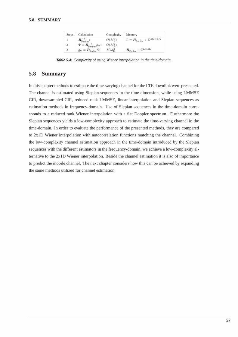
5.8. SUMMARY
Steps Calculation Complexity Memory
1 R−1
gmrgmr: O(M3
R) Γ = Rgmrgmr ∈ CMR×MR
2 Φ = R−1
gmrgmrgmr: O(M2
R)
3 gm = RgmgmrΦ: MM2
R Rgmgmr ∈ CL×MR
Table 5.4: Complexity of using Wiener interpolation in the time-domain.
5.8 Summary
In this chapter methods to estimate the time-varying channel for the LTE downlinkwere presented.
The channel is estimated using Slepian sequences in the time-dimension, while using LMMSE
CIR, downsampled CIR, reduced rank LMMSE, linear interpolation and Slepian sequences as
estimation methods in frequency-domain. Use of Slepian sequences in the time-domain corre-
sponds to a reduced rank Wiener interpolation with a flat Doppler spectrum.Furthermore the
Slepian sequences yields a low-complexity approach to estimate the time-varyingchannel in the
time-domain. In order to evaluate the performance of the presented methods,they are compared
to 2x1D Wiener interpolation with autocorrelation functions matching the channel. Combining
the low-complexity channel estimation approach in the time-domain introduced by theSlepian
sequences with the different estimators in the frequency-domain, we achieve a low-complexity al-
ternative to the 2x1D Wiener interpolation. Beside the channel estimation it is also of importance
to predict the mobile channel. The next chapter considers how this can be achieved by expanding
the same methods utilized for channel estimation.
57

CHAPTER 5. TIME-VARYING CHANNEL ESTIMATION
58

Channel Prediction 6
In Chapter 5 the channel estimation problem was considered, now channel prediction is investi-
gated. The NodeB schedules resource blocks to the UEs for the each subframe. The scheduling is
based on the state of the channel, reported by the UE in a frequency division duplex (FDD) system.
However for mobile users at vehicular speed the channel state informationgets outdated, hence
the channel must be predicted for a proper scheduling [20]. This chapter introduces a method to
predict the channel in UMTS LTE using Slepian sequences developed by[27].
6.1 Prediction using Slepian Sequences
As stated in Chapter 5 the utilization of Slepian sequences results in a time-concentrated and band-
limited sequence. For prediction purposes channel estimates forℓ > M − 1 are calculated. We
denote the prediction as minimum-energy prediction since the Slepian sequences are concentrated
in the intervalm ∈ IM . The used Slepian sequences for channel estimation purpose were defined
for m ∈ IM , hence the first task is to obtain Slepian sequences at timesℓ > M − 1.
6.1.1 Minimum Energy Band-Limited Sequences
By evaluating (5.4) in Section 5.2, basis vectorsui were calculated for a block of finite length, i.e.
ui[m] for m ∈ IM . The sequenceui[m] can be continued form overZ in a minimum energy
(ME) band-limited sense by evaluating (5.4) on the right hand side, as expressed in (6.1) [27].
ui[ℓ,W, M ] =M−1∑
m=0
sin(2πνDmax(m − ℓ))
π(m − ℓ)ui[m,W, M ]
1
λi(W, M). (6.1)
The value forui[ℓ] at ℓ /∈ I can be calculated since the sequenceui[m] for m ∈ I andλi are
already known.
6.1.2 Prediction
Using the minimum energy band-limited sequences and the same weightingγ as for the channel
estimation, the ME band-limited prediction of a time-variant channel for anym ∈ Z is finally

CHAPTER 6. CHANNEL PREDICTION
given as
g[ℓ] =D−1∑
i=0
ui[l]γi, (6.2)
whereui[ℓ] is the extended basis sequence at time indicesℓ ≥ M .Using the same methods as
for channel estimation (Chapter 5), the channel can be predicted with the new knowledge from
Section 6.1.1 and (6.2).
6.2 Wiener Predictor
Another solution for channel prediction is the Wiener predictor, which requires information about
the second order statistics of the channel.
The structure of the Wiener predictor is based on Wiener interpolation as described in (6.3). For a
sequencegmr[m] with m ∈ IM the predicted value at time indexℓ > M − 1 is as follows,
g[ℓ] = rgmgmrH [ℓ]R−1
gmrgmrgmr, (6.3)
wherergmgmr[m] is found the same way as in (5.47). The Wiener predictor can be approximated
by a reduced rank predictor where subspaces with small eigenvalues are truncated [27].
6.3 Relation Between Wiener Predictor and ME Predictor
In [27] it is shown that a reduced rank Wiener predictor approximates theWiener predictor. Using
the same procedure as in Section 5.6 but replacing time indexm with an indexℓ greater than
the block size (ℓ > M − 1), shows that ME band-limited prediction and reduced rank Wiener
prediction assuming a constant Doppler spectrum spans the same subspace.
6.4 Summary
Using Slepian sequences it is possible to perform channel prediction such that the information
about the channel is not outdated at NodeB. Furthermore the use of Slepian sequences for predic-
tion is similar to the reduced rank Wiener prediction.
60

Simulation Results 7
The presented estimation and prediction methods are now simulated using Matlab.The written
Matlab files can be found on the companion CD-ROM. The LTE downlink signal structure and
SCME model offer several parameters to adjust. It was chosen to work with the downlink trans-
mission bandwidths of 2.5 and 20 MHz, since the first use the same sampling frequency as the
current UMTS 3G system while the latter is the maximum transmission bandwidth.
7.1 SCME Channel Model Configuration
The SCME channel model was used to generate channel realizations. Inorder to adjust it to the
LTE downlink simulation, the model has to be configured appropriately.
7.1.1 Generation of Impulse Response
The SCME model takes several inputs which are described in [21]. A channel has to be gener-
ated for each OFDM symbol, which has a duration ofTs as described in Section 3.3.2. [21] does
not give a detailed description of how to configure the model according thementioned problem.
Therefore the solution to this is given in this section.
In light of line 531in the Matlab file’scm.m’ within the SCME package, the channel impulse re-
sponse is generated for each OFDM symbol by configuring the parameterscmpar.SampleDensity
as follows,
SlotDuration=0.5e-3; %0.5 ms
N.OFDM_symbol_pr_slot=6; % 6 symbols pr. slot
speed_of_light=2.99792458e8; %m/s
fcarrier=2e9; % 2GHz carrier frequency
wavelength=speed_of_light/fcarrier;
delta_t=SlotDuration/N.OFDM_symbol_pr_slot; %OFDM symbol duration
linkpar.MsVelocity=channel.vmax; % Velocity of UE is configured
%Configuring parameter to generate impulse response for each OFDM symbol.
scmpar.SampleDensity = wavelength / (linkpar.MsVelocity*2*delta_t);

CHAPTER 7. SIMULATION RESULTS
The parameterscmpar.SampleDensitydetermines the delay between the generation of each
channel impulse response.
7.2 Autocorrelation of Doppler Shift
Since some properties such as the power delay profile of the SCME model are unknown, they are
determined by simulations. The SCME generates a number of impulse responsesfor each new
channel generation.
For each channel generation the autocorrelation for each tap is found.The autocorrelation repre-
sents the correlation caused by the specific Doppler shifts of the generated channel. Let us denote
the autocorrelation by vectorr, normalized such thatr[0] = 1. The simulations are run over 4000
generated channels with each 100 impulse responses. Hereafter the correlation is averaged and
the result is depicted on Figure 7.1. The autocorrelation vector is used as the a-priori Doppler
0 10 20 30 40 50 60 70 80 90 100−0.4
−0.2
0
0.2
0.4
0.6
0.8
1
lag [k]
r[k]
Figure 7.1: Autocorrelation for the SCME channel model. The correlation is averaged over 4000 generated
channels as well as over all taps.
autocorrelation when the Wiener interpolator is used (see Section 5.5.2). The power delay profile
is found as an average of power delay profiles from 2000 generated channels.
Figure 7.2 shows the power delay profile for 20 MHz transmission bandwidth. The chosen
number of taps for this transmission bandwidth is 27.
7.3 Simulation Scenarios
In Chapter 5 different low-complexity estimation methods were presented forthe time-varying
channel. The utilized methods are as follows,
- LMMSE CIR estimator and downsampled CIR estimator:
62
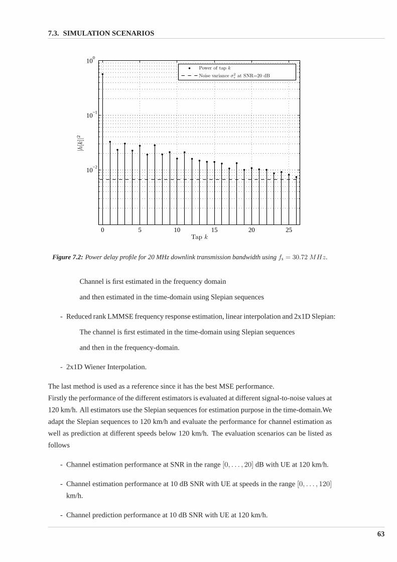
7.3. SIMULATION SCENARIOS
0 5 10 15 20 25
10−2
10−1
100
Tap k
|h[k
]|2Power of tap k
Noise variance σ2
zat SNR=20 dB
Figure 7.2: Power delay profile for 20 MHz downlink transmission bandwidth usingfs = 30.72 MHz.
Channel is first estimated in the frequency domain
and then estimated in the time-domain using Slepian sequences
- Reduced rank LMMSE frequency response estimation, linear interpolation and 2x1D Slepian:
The channel is first estimated in the time-domain using Slepian sequences
and then in the frequency-domain.
- 2x1D Wiener Interpolation.
The last method is used as a reference since it has the best MSE performance.
Firstly the performance of the different estimators is evaluated at different signal-to-noise values at
120 km/h. All estimators use the Slepian sequences for estimation purpose in thetime-domain.We
adapt the Slepian sequences to 120 km/h and evaluate the performance forchannel estimation as
well as prediction at different speeds below 120 km/h. The evaluation scenarios can be listed as
follows
- Channel estimation performance at SNR in the range[0, . . . , 20] dB with UE at 120 km/h.
- Channel estimation performance at 10 dB SNR with UE at speeds in the range [0, . . . , 120]
km/h.
- Channel prediction performance at 10 dB SNR with UE at 120 km/h.
63

CHAPTER 7. SIMULATION RESULTS
- Channel prediction performance at 10 dB SNR with UE at speeds in the range[0, . . . , 120]
km/h.
In order to evaluate the performance we apply the 2.5 MHz and 20 MHz transmission bandwidths
within the UMTS LTE. The SNR level at 10 dB is chosen since this is a typical value for wireless
communications.
7.4 Evaluation
We apply the same procedure to investigate the 2.5 MHz bandwidth as for the 20MHz bandwidth.
The used parameters are listed in Table 7.1. The power delay profile for 2.5MHz transmission
bandwidth is depicted on Figure 3.3. For each OFDM symbol, the estimated frequency response
Parameters Values
Channel model Urban macro
Number of simulations 400
Taps 12 (27)
Cyclic Prefix Long
Block size 48 OFDM symbols
Sampling frequency 3.84 MHz (30.72 MHz)
DimensionD for Slepian Sequences in time-domain 4 (5)
Speed of UE 120 km/h
DimensionDf of Slepian sequences in frequency-domain 12 (27)
Table 7.1: Parameters used in simulation for 2.5 MHz and 20 MHz downlinktransmission bandwidth. For
the latter case the changed parameters are specified in the round brackets.
of the channel is compared to the true frequency response. The true frequency response is found
as the Fourier transform of the channel impulse response. The performance of the estimators
is measured in the MSE (mean square error) sense between the true channel and the estimated
channel. The frequency response is compared in the range of the usedsubcarriers (see also Figure
2.2), since the estimates are used for these positions only.
7.4.1 Performance at Different SNR
The achieved mean square error for different SNR values are depicted on Figure 7.3 for 2.5 MHz
transmission bandwidth and on Figure 7.4 for the 20 MHz bandwidth. The simulations are always
conducted over 400 different channel iterations.
For the 2.5 MHz transmission bandwidth it is noticeable that the performance ofLMMSE CIR
estimator is close to the Wiener Interpolator. The downsampled CIR estimator again performs as
well as LMMSE CIR for SNR up to 10 dB, hereafter the performance decreases. The reduced
performance is caused by the aliasing due to the downsampling as describedin Section 4.4.3. The
64
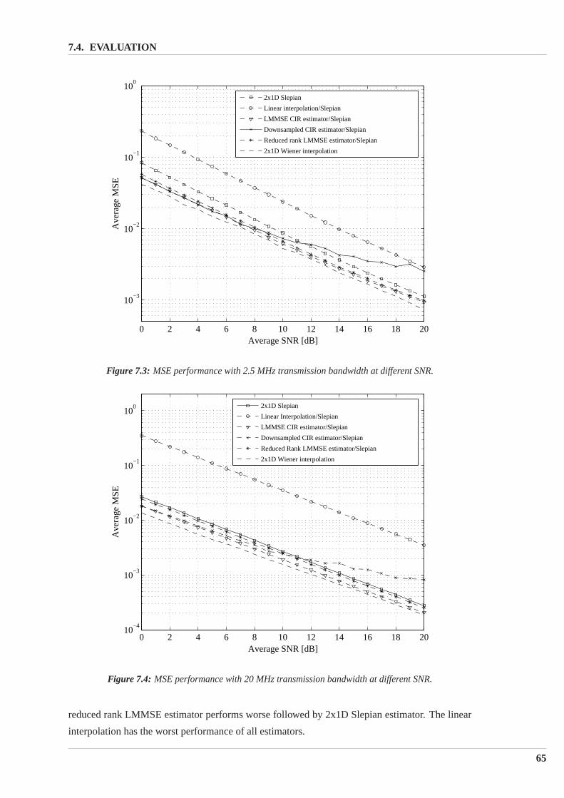
7.4. EVALUATION
0 2 4 6 8 10 12 14 16 18 20
10−3
10−2
10−1
100
Average SNR [dB]
Ave
rage
MS
E
2x1D Slepian
Linear interpolation/Slepian
LMMSE CIR estimator/Slepian
Downsampled CIR estimator/Slepian
Reduced rank LMMSE estimator/Slepian
2x1D Wiener interpolation
Figure 7.3: MSE performance with 2.5 MHz transmission bandwidth at different SNR.
0 2 4 6 8 10 12 14 16 18 2010
−4
10−3
10−2
10−1
100
Average SNR [dB]
Ave
rage
MS
E
2x1D Slepian
Linear Interpolation/Slepian
LMMSE CIR estimator/Slepian
Downsampled CIR estimator/Slepian
Reduced Rank LMMSE estimator/Slepian
2x1D Wiener interpolation
Figure 7.4: MSE performance with 20 MHz transmission bandwidth at different SNR.
reduced rank LMMSE estimator performs worse followed by 2x1D Slepian estimator. The linear
interpolation has the worst performance of all estimators.
65
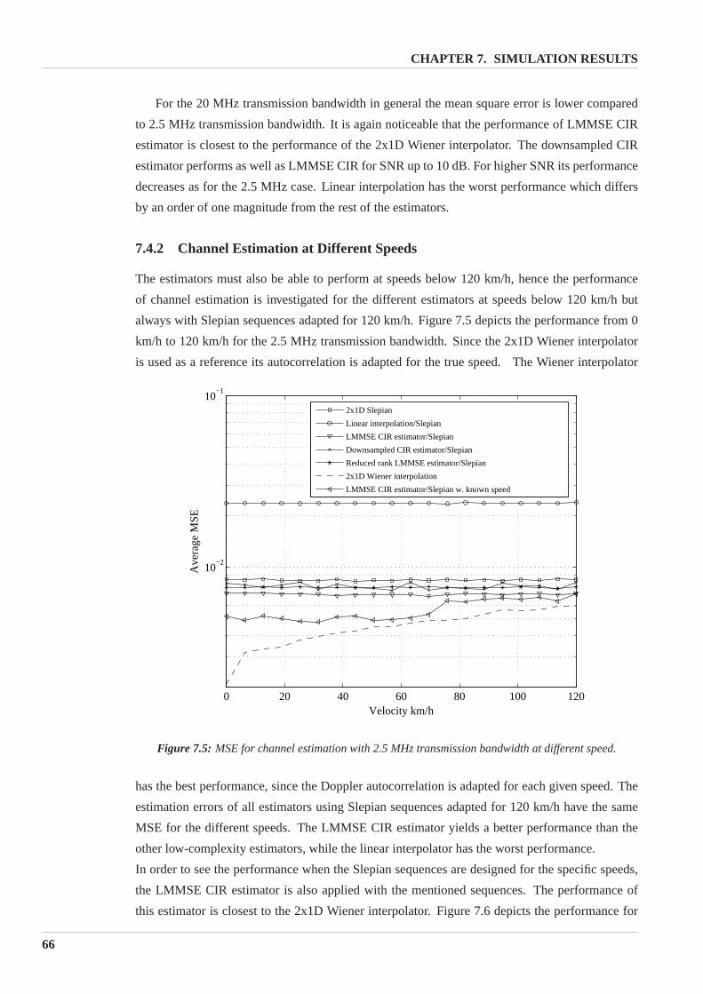
CHAPTER 7. SIMULATION RESULTS
For the 20 MHz transmission bandwidth in general the mean square error is lower compared
to 2.5 MHz transmission bandwidth. It is again noticeable that the performanceof LMMSE CIR
estimator is closest to the performance of the 2x1D Wiener interpolator. The downsampled CIR
estimator performs as well as LMMSE CIR for SNR up to 10 dB. For higher SNR its performance
decreases as for the 2.5 MHz case. Linear interpolation has the worst performance which differs
by an order of one magnitude from the rest of the estimators.
7.4.2 Channel Estimation at Different Speeds
The estimators must also be able to perform at speeds below 120 km/h, hencethe performance
of channel estimation is investigated for the different estimators at speeds below 120 km/h but
always with Slepian sequences adapted for 120 km/h. Figure 7.5 depicts theperformance from 0
km/h to 120 km/h for the 2.5 MHz transmission bandwidth. Since the 2x1D Wiener interpolator
is used as a reference its autocorrelation is adapted for the true speed. The Wiener interpolator
0 20 40 60 80 100 120
10−2
10−1
Velocity km/h
Ave
rage
MS
E
2x1D Slepian
Linear interpolation/Slepian
LMMSE CIR estimator/Slepian
Downsampled CIR estimator/Slepian
Reduced rank LMMSE estimator/Slepian
2x1D Wiener interpolation
LMMSE CIR estimator/Slepian w. known speed
Figure 7.5: MSE for channel estimation with 2.5 MHz transmission bandwidth at different speed.
has the best performance, since the Doppler autocorrelation is adapted for each given speed. The
estimation errors of all estimators using Slepian sequences adapted for 120km/h have the same
MSE for the different speeds. The LMMSE CIR estimator yields a better performance than the
other low-complexity estimators, while the linear interpolator has the worst performance.
In order to see the performance when the Slepian sequences are designed for the specific speeds,
the LMMSE CIR estimator is also applied with the mentioned sequences. The performance of
this estimator is closest to the 2x1D Wiener interpolator. Figure 7.6 depicts the performance for
66

7.4. EVALUATION
0 20 40 60 80 100 120
10−4
10−3
10−2
10−1
Velocity km/h
Ave
rage
MS
E
2x1D Slepian
Linear interpolation/Slepian
LMMSE CIR estimator/Slepian
Downsampled CIR estimator/Slepian
Reduced rank LMMSE estimator/Slepian
2x1D Wiener interpolation
LMMSE CIR estimator/Slepian w. known speed
Figure 7.6: MSE for channel estimation with 20 MHz transmission bandwidth at different speeds.
the 20 MHz transmission bandwidth. In this case the MSE of all estimators are lower compared
to 2.5 MHz transmission bandwidth. The Wiener interpolator has the lowest MSE, while the
estimation errors of all estimators using Slepian sequences adapted for 120km/h have the same
MSE for the different speeds. We again apply the LMMSE CIR estimator with the adapted Slepian
sequences for the different speeds. The performance of this estimatoris closest to the 2x1D Wiener
interpolator.
7.4.3 Channel Prediction
As mentioned in Chapter 6 channel prediction is also necessary. The prediction horizon is chosen
as 2 subframes, i.e. 24 OFDM symbols and the number OFDM symbols over which the estimation
is performed is stillM = 48. Figure 7.7 depicts the measured MSE for 2.5 MHz transmission
bandwidth. The channel is predicted for a UE with velocity 120 km/h. Since thechannel is
predicted afterm = 47, the MSE is lower atm < 48 because the channel is estimated for this
interval, while the MSE increases sharply afterm = 47 because of the channel is now predicted. In
general all estimators, except the linear interpolation, have the same MSE for channel prediction,
however the downsampled CIR estimator has the performance closest to the Wiener predictor. The
MSE performance for 20 MHz bandwidth is depicted on Figure 7.8. In this case the individual
performance of the estimators are in general the same as for 2.5 MHz transmission bandwidth.
The downsampled CIR estimator has the same performance for prediction as the other estimators.
The resulting MSE increases sharply afterm = 47. All predicted values have in general the same
67

CHAPTER 7. SIMULATION RESULTS
0 10 20 30 40 50 60 70 80
10−2
10−1
100
OFDM symbol m
Ave
rage
MSE
2x1D Slepian
Linear interpolation/Slepian
LMMSE CIR estimator/Slepian
Downsampled CIR estimator/Slepian
Reduced rank LMMSE estimator/Slepian
2x1D Wiener interpolation
LMMSE CIR estimator/Slepian w. known speed
Figure 7.7: MSE for channel prediction with 2.5 MHz transmission bandwidth at 120 km/h. The prediction
starts after the thick vertical black line atm = 47. The 2x1D Wiener interpolator apply prediction for
m > 47 and estimation otherwise.
0 10 20 30 40 50 60 70 8010
−3
10−2
10−1
100
101
OFDM symbol m
Ave
rage
MSE
2x1D Slepian
Linear interpolation/Slepian
LMMSE CIR estimator/Slepian
Downsampled CIR estimator/Slepian
Reduced rank LMMSE estimator/Slepian
2x1D Wiener interpolation
LMMSE CIR estimator/Slepian w. known speed
Figure 7.8: MSE for channel prediction with 20 MHz transmission bandwidth at 120 km/h. The channel
is predicted afterm = 47.The 2x1D Wiener interpolator apply prediction form > 47 and estimation
otherwise.
68

7.4. EVALUATION
MSE. Excecpt for the linear interpolation the prediction error has its maximum at m = 71. This
is the maximum horizon at which we can predict. This prediction horizonℓ = 24 corresponds to
a covered distance in wavelengthλ,
d =vmaxℓTs
c0/fc=
7
16λ, (7.1)
by the UE. Hence we can predict the channel for a movement of maximum716λ of the wavelength
λ = c0/fc. It should be noted that we only calculate the distance at which we have the maximum
prediction error. For practical usage the distance, i.e. the prediction horizon may be reduced.
7.4.3.1 Channel Prediction at Different Speeds
As for the channel estimation in Section 7.4.2 we investigate the performance ofchannel prediction
at speeds below 120 km/h. The Slepian sequence used in time-domain is adapted for 120 km/h.
The prediction is performed for OFDM symbolm = 59, i.e. the horizon is one subframe (12
OFDM symbols). Figure 7.9 depicts the MSE for the 2.5 MHz transmission bandwidth. As for
0 20 40 60 80 100 12010
−3
10−2
10−1
100
Velocity km/h
Ave
rage
MS
E
2x1D Slepian
Linear interpolation/Slepian
LMMSE CIR estimator/Slepian
Downsampled CIR estimator/Slepian
Reduced rank LMMSE estimator/Slepian
LMMSE CIR estimator/Slepian w. known speed
2x1D Wiener Interpolation
Figure 7.9: MSE for channel prediction with 2.5 MHz at different speeds.
the estimation case the prediction errors have the MSE for the estimators with Slepian sequences
adapted for 120 km/h through out the range of chosen speeds. The downsampled CIR estimator
has the lowest MSE compared to the other low-complexity estimators. Figure 7.10depicts the
same scenario for the 20 MHz transmission bandwidth. For this transmission bandwidth it is not
possible to discriminate between the performance of the low-complexity estimators. Again the
prediction errors have the MSE for the estimators with Slepian sequences adapted for 120 km/h.
69

CHAPTER 7. SIMULATION RESULTS
0 20 40 60 80 100 12010
−4
10−3
10−2
10−1
100
Velocity km/h
Ave
rage
MS
E
2x1D Slepian
Linear interpolation/Slepian
LMMSE CIR estimator/Slepian
Downsampled CIR estimator/Slepian
Reduced rank LMMSE estimator/Slepian
2x1D Wiener interpolation
LMMSE CIR estimator/Slepian w. known speed
Figure 7.10: MSE for prediction with 20 MHz transmission bandwidth at different speeds.
However if the speed is known as for the LMMSE estimator using Slepian sequences adapted to
the speed then the achieved MSE is lower and closest to the Wiener predictor.
7.5 Summary
The performance of the presented methods for time-variant channel estimation has been simulated
with the SCME channel model. The autocorrelation of the Doppler spectrum from the SCME
model is found numerically. The different estimators have been evaluated at 2.5 MHz and 20 MHz
downlink transmission bandwidths. All estimators are compared to the 2x1D Wiener interpolation
which is used as reference since it consistently yields the lowest MSE. In general the LMMSE
CIR estimator using Slepian sequences shows the best MSE performance of all estimators, since
it is closest to the 2x1D Wiener interpolator. Furthermore it is shown that the prediction horizon
for 2.5 MHz as well as 20 MHz transmission bandwidths corresponds to a covered distance of
approximately one half of the wavelengthλ at 120 km/h.
70
Conclusion and Future Work 8
In order to ensure competitiveness for the next few years a long-term evolution of the 3GPP radio-
access technology is currently developed. In this thesis important properties of the physical layer
in UMTS-LTE downlink have been investigated based on specifications in Release 7 and on work-
ing assumptions in Release 8.
OFDMA is utilized as multiple access scheme in the downlink. One of the most importantaspects
in an OFDM system is a reliable and accurate channel estimation.
In order to perform realistic simulations, channel models with time-invariant and time-varying be-
havior have been investigated. The chosen channel model is the Spatial Channel Model Extended
(SCME), which generates channel coefficients based on 3GPP channel model specifications. The
channel model supports a typical urban area scenario as well as mobility of the UE. The SCME
model is implemented with the LTE downlink structure in Matlab.
Different low-complexity estimation methods have been presented, all basedon Slepian sequences.
The channel is estimated using Slepian sequences in the time-dimension, while using LMMSE
CIR estimator, downsampled CIR estimator, reduced rank LMMSE estimator, linear interpolation
and also Slepian sequences as estimation method in the frequency-domain.
The LMMSE CIR and downsampled CIR present a way to estimate the channelimpulse response
based on assumptions of the number of tapsL. The downsampled CIR furthermore makes use of
the fact that the LTE downlink only occupies2/3 of the bandwidth.
The complexity of the algorithms have been reviewed and it is shown that the reduced rank
LMMSE has the highest complexity, followed by LMMSE CIR estimator and downsampled CIR
estimator respectively.
In order to investigate the performance of the presented methods, they arecompared to 2x1D
Wiener interpolation with perfectly known autocorrelation functions. Using Slepian sequences
it is also possible to perform channel prediction in a minimum-energy (ME) band-limited sense
such that the information about the channel does not get outdated at the NodeB. It is shown that
the maximum prediction horizon at 120 km/h corresponds to a covered distance of one half of
the wavelength. Using Slepian sequences for channel estimation as well asprediction in time-
domain is similar to the reduced rank Wiener interpolation and prediction respectively with uni-
form Doppler spectrum assumption, since the subspaces spanned by both estimators are exactly

CHAPTER 8. CONCLUSION AND FUTURE WORK
the same. The performance of the presented methods for time-varying channel estimation has been
evaluated with the SCME channel model. The 2.5 MHz and 20 MHz downlink transmission band-
widths within the LTE have been investigated. It has been shown that the LMMSE CIR estimator
with the Slepian sequence in general has the MSE performance, since it is closest to the Wiener
interpolator. Hence the LMMSE CIR estimator is a good compromise between complexity and
performance.
Future work
This thesis investigated channel estimators for the UMTS LTE downlink structure with transmis-
sion bandwidths 2.5 MHz and 20 MHz. For future research with other transmission bandwidths the
implemented Matlab simulator can easily be reconfigured to evaluate the estimation performance.
We have not considered coding in this thesis, hence this is left as future work. The different low-
complexity estimators developed in this project can be used with the applied coding in order to
find an appropriate estimator. Moreover the evaluation of the estimators shows that if the speed of
the UE is below the speed at which the Slepian sequences are adapted, the performance decreases
with respect to the Wiener interpolator. Hence possible future work is also toestimate the speed of
the UE in order to improve the channel estimation as well as prediction. This work can be based
on [27] which already presents an approach for this task.
72
Bibliography
[1] 3GPP. 3GPP TR 25.913 V7.3.0 Requirements for Evolved UTRA (E-UTRA) and Evolved
UTRAN (E-UTRAN) . Technical report, 3GPP, September 2003.
[2] 3GPP. 3GPP TR 25.996 V6.1.0 Spatial Channel Model for Multiple Input Multiple Output
(MIMO) simulations (Release 6). Technical report, 3GPP, September 2003.
[3] 3GPP. 3GPP TR 25.943 V6.0.0 Deployment Aspects (Release 6). Technical report, 3GPP,
December 2004.
[4] 3GPP. 3GPP TR 25.814 V7.1.0 Physical Layer Aspects for Evolved Universal Terrestrial
Radio Access (UTRA) (Release 7). Technical report, 3GPP, September 2006.
[5] 3GPP. 3GPP TS 36.211 V0.3.1 Physical Channels and Modulation (Release 8). Technical
report, 3GPP, February 2007.
[6] Andrea Ancora, Calogero Bona, and Dirk T M Slock. Down-sampledImpulse Response
Least-Squares Channel Estimation for LTE OFDMA. InICASSP 2007, 32nd IEEE Interna-
tional Conference on Acoustics, Speech, and Signal Processing, Honolulu, USA, Apr 2007.
[7] P. Dent, G.E. Bottomley, and T. Croft. Jakes fading model revisited. InElectronics Letters,
volume 29, pages 1162–1163, 24 June 1993.
[8] O. Edfors, M. Sandell, J. van de B., B. Wilson, and P. Börjesson. OFDM Channel Estimation
by Singular Value Decomposition. InIEEE Vehicular Technology Conference, Atlanta, USA,
pp. 923-927,April 28-May 1., 1996.
[9] B.H. Fleury. An Uncertainty Relation for WSS Processes and Its Application to WSSUS
Systems.IEEE Transactions on Communications, 44(12):1632–1634, Dec. 1996.
[10] G. H. Golub and C. F. Van Loan.Matrix Computations. Baltimore, MD, USA, second
edition, 1989.
[11] S Haykin.Adaptive Filter Theory. Prentice-Hall, Inc., Upper Saddle River, NJ, USA, 1995.
[12] Harri Holma and Antti Toskala.WCDMA for UMTS. John Wiley & Sons, Inc., New York,
NY, USA, 2002.

BIBLIOGRAPHY
[13] Stefan Kaiser.Multi-Carrier CDMA Mobile Radio Systems – Analysis and Optimization of
Detection, Decoding, and Channel Estimation. PhD thesis, University of Kaiserslautern,
Germany, January 1998. VDI Verlag Düsseldorf, Series 10, No. 531, ISBN 3-18-353110-0.
[14] Steven M. Kay.Fundamentals of Statistical Signal Processing: Estimation Theory. Prentice-
Hall, Inc., Upper Saddle River, NJ, USA, 1993.
[15] Louis Litwin and Michael Pugel. The principles of OFDM, January 2001.
[16] Andrew M. Odlyzko. Internet traffic growth: Sources and implications, 2003.
[17] Alan V. Oppenheim and Ronald W. Schafer.Digital Signal Processing. Prentice–Hall, 1989.
[18] M.K. Ozdemir, H. Arslan, and E. Arvas. Adaptive Low-Rank MIMO-OFDM Channel Es-
timation. InWireless and Microwave Technology, 2005. WAMICON 2005. The 2005IEEE
Annual Conference, page 5pp., 2005.
[19] S. Parkvall, E. Englund, M. Lundevall, and J. Torsner. Evolving3G Mobile Systems: Broad-
band and Broadcast Services in WCDMA.IEEE Communications Magazine, 44(2):30–36,
Feb. 2006.
[20] A. Pokhariyal, G. Monghal, K. I. Pedersen, P. E. Mogensen, I. Z. Kovacs, C. Rosa, and T. E.
Kolding. Frequency Domain Packet Scheduling Under Fractional Load for the UTRAN LTE
Downlink. In Vehicular Technology Conference, 2007. VTC2007-Spring. IEEE 65th, pages
699–703, April 2007.
[21] Jari Salo, Giovanni Del Galdo, Jussi Salmi, Pekka Kyösti, Marko Milojevic, Daniela Laselva,
and Christian Schneider. MATLAB implementation of the 3GPP Spatial ChannelModel
(3GPP TR 25.996). On-line, January 2005. http://www.tkk.fi/Units/Radio/scm/.
[22] D. Slepian. Prolate spheroidal wave functions, Fourier analysis,and uncertainty. V - The
discrete case.AT&T Technical Journal, 57:1371–1430, June 1978.
[23] Antti Toskala, Harri Holma, Kari Pajukoski, and Esa Tiirola. Utran Long Term Evolution
in 3GPP. InIEEE 17th International Symposium on Personal, Indoor and Mobile Radio
Communications, pages 1–5, Sept. 2006.
[24] J.-J. van de Beek, O. Edfors, M. Sandell, S.K. Wilson, and P.O. Borjesson. On Channel
Estimation in OFDM Systems. InIEEE 45th Vehicular Technology Conference, volume 2,
pages 815–819vol.2, 25-28 July 1995.
[25] T. Zemen, H. Hofstetter, and G. Steinbock. Successive Slepian Subspace Projection in Time
and Frequency for Time-Variant Channel Estimation, 2005.
[26] T. Zemen and C.F. Mecklenbrauker. Time-Variant Channel EstimationUsing Discrete Pro-
late Spheroidal Sequences.IEEE Transactions on Signal Processing,, 53(9):3597–3607,
Sept. 2005.
74

BIBLIOGRAPHY
[27] T. Zemen and Fleury B. H. Mecklenbrauker, Kaltenberger F. Minimum-Energy Band-
Limited Predictor with Dynamic Subspace Selection for Time-Variant Flat-FadingChannels.
IEEE Transactions on Signal Processing, 2007. Accepted (2006-12-06), to be published.
[28] Thomas Zemen.OFDM Multi-User Communication Over Time-Variant Channels. PhD
thesis, 2004. ISBN 3-902477-04-0.
75


Orthogonal Frequency Division
Multiplexing systemsA
In high data rate, wideband communication through multipath fading channel, thereceived signals
are affected by inter-symbol interference (ISI) due to the fact that thetime spread of the channel is
relatively large compared to the symbol duration. Reducing ISI is an important issue for enhancing
the quality of wideband communications.
Normally ISI is removed by channel equalization, which is implemented either in thetime or
frequency domain, with symbol-by-symbol or sequence estimation algorithms.
If the symbol rate is reduced, while the information rate is remained, the impact ofISI becomes
negligible and equalization becomes unnecessary. One method is to increasethe constellation size
in an Q-ary pulse modulation scheme. However, there is a limit on how largeQ can be before
modulation and demodulation becomes too complex.
Multicarrier modulation offers another approach. A serial high rate data stream is distributed into
many parallel low rate data streams, transmitted through many orthogonal narrowband subcarriers,
thus the symbol duration in each channel is large enough that the ISI can be negligible.
In this Appendix, the principle of multicarrier modulation is reviewed, followed by a review of
OFDM, which is based on [15].
A.1 Multicarrier Modulation System
The concept of multicarrier modulation is illustrated in Figure A.1. The idea is to divide the trans-
mitted bitstream into many different substreams and send them over many different subcarriers.
The data rate on each of the subcarriers is less than the total data rate, andthe corresponding sub-
carrier bandwidth is less than the total system bandwidth. Multicarrier modulationcan be seen
as a parallel transmission scheme developed to eliminate ISI by extending the symbol interval.
However, parallel transmission requires separate modulation and demodulation for each subcar-
rier. High data rate transmission requires a large number of subcarriers,which makes the imple-
mentation of multicarrier transmitter and receiver complex. A more feasible way toimplement
multicarrier modulation leads to the concept of OFDM.

APPENDIX A. ORTHOGONAL FREQUENCY DIVISION MULTIPLEXING SYSTEMS
Figure A.1: Basic structure of multicarrier modulation system. ’PS’ isthe pulse shaping filter at the
transmitter side, while ’MF’ is the matched filter at receiver side.
A.2 Concept of OFDM System
OFDM is a feasible method to implement multicarrier modulation scheme which combats theISI
in multipath fading channel with spectral efficiency.
As mentioned above, the requirement for separate modulator and demodulator on each subcarrier
is complex to be implemented. OFDM makes the modulation in parallel transmission be easily
implemented. In OFDM, spectrum efficiency is increased by the fact that thespectrums of the
subcarriers overlap, as shown in Figure A.3. The information transmitted over the carriers can still
be separated because they are orthogonal. The orthogonal carrierscan be created using inverse fast
Fourier transformation ((IFFT)). The frequency spacing between thesubcarriers is determined by
the sampling frequencyfs and the number of points,NIFFT, in the IFFT.
fspace=fs
NIFFT(A.1)
A.3 Orthogonality
An OFDM system is shown in Figure A.2. The Fast Fourier Transform (FFT) algorithms are used
to generate orthogonal subcarriers due to their computational efficiency[15]. The IFFT operation
results in the composite OFDM symbol of durationTs. The idea behind using IFFT to modulate
78
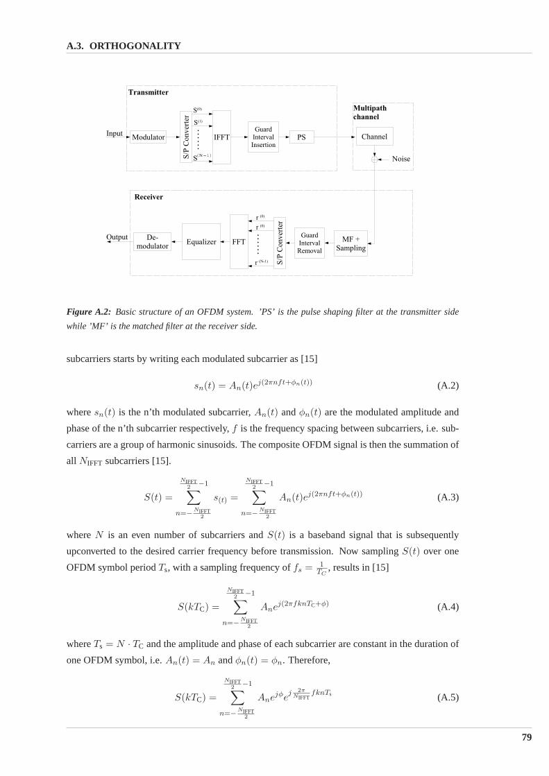
A.3. ORTHOGONALITY
Figure A.2: Basic structure of an OFDM system. ’PS’ is the pulse shaping filter at the transmitter side
while ’MF’ is the matched filter at the receiver side.
subcarriers starts by writing each modulated subcarrier as [15]
sn(t) = An(t)ej(2πnft+φn(t)) (A.2)
wheresn(t) is the n’th modulated subcarrier,An(t) andφn(t) are the modulated amplitude and
phase of the n’th subcarrier respectively,f is the frequency spacing between subcarriers, i.e. sub-
carriers are a group of harmonic sinusoids. The composite OFDM signal isthen the summation of
all NIFFT subcarriers [15].
S(t) =
NIFFT2
−1∑
n=−NIFFT2
s(t) =
NIFFT2
−1∑
n=−NIFFT2
An(t)ej(2πnft+φn(t)) (A.3)
whereN is an even number of subcarriers andS(t) is a baseband signal that is subsequently
upconverted to the desired carrier frequency before transmission. Now samplingS(t) over one
OFDM symbol periodTs, with a sampling frequency offs = 1TC
, results in [15]
S(kTC) =
NIFFT2
−1∑
n=−NIFFT2
Anej(2πfknTC+φ) (A.4)
whereTs = N · TC and the amplitude and phase of each subcarrier are constant in the duration of
one OFDM symbol, i.e.An(t) = An andφn(t) = φn. Therefore,
S(kTC) =
NIFFT2
−1∑
n=−NIFFT2
Anejφej 2π
NIFFTfknTs (A.5)
79

APPENDIX A. ORTHOGONAL FREQUENCY DIVISION MULTIPLEXING SYSTEMS
Comparing with the IDFT equation [17],
S(kTC) =
NIFFT2
−1∑
n=−NIFFT2
Anejφej 2π
NIFFTkn
(A.6)
shows that both equations are equal iff = 1Ts
. This condition ensures that allN subcarriers are
orthogonal. Orthogonality is clear from examining the spectrum of the OFDM signal in Figure
A.3. The IFFT block samples the spectrum at the peak of each sinc functionto mapAn andφn to
subcarriers. This results in no interference between subcarriers. The overlapping spectra is not of
importance because the peak of each sinc functions coincides with zero crossings of all other sinc
functions. In the time domain, orthogonality means that all subcarriers have an integer multiple of
periods in each symbol periodTs as shown in Figure A.4.
0 2 4 6 8 10−0.4
−0.2
0
0.2
0.4
0.6
0.8
1
1.2
f
subcarrier 1 subcarrier N
IFFT sampling points
Figure A.3: The spectrum of an OFDM signal consists of overlapping sinc functions. Each sinc function is
sampled at its peak, which coincides with zero crossings of all other functions [15].
A.4 Advantages of OFDM
A.4.1 Immunity to Frequency Selective Fading
Because of the nature of a mobile environment, multiple delays of the transmitted signal reach a
mobile receiver. Delay spread results in a frequency selective fading channel response. Hence,
some signal frequencies are enhanced while others suffer from deepfades. This affects both the
amplitude and phase modulation of the carrier and consequently results in information loss. In
order to combat frequency selective fading, OFDM uses a signal bandwidth that is much smaller
than the coherence bandwidth associated with the estimated delay spread of the channel. This
80

A.5. IMMUNITY TO INTER-SYMBOL INTERFERENCE
0 50 100 150 200 250 300−1
−0.8
−0.6
−0.4
−0.2
0
0.2
0.4
0.6
0.8
1
t
Figure A.4: Orthogonality in the time domain means that all subcarriersin an OFDM signal have an
integer number of periods during the period of one OFDM symbol [15].
way, each subcarrier experiences fading and only some bits are lost if some of the subcarriers
experience deep fades [15].
A.5 Immunity to Inter-Symbol Interference
In OFDM, dividing the incoming bit stream overN subcarriers increases the symbol duration by
a factor ofN . The symbol period is made greater than the delay spread of the channel. This way
the effect of ISI is restricted to one symbol duration only, and only the first few samples of each
period are distorted. Furthermore, to avoid such distortion, OFDM can usea cyclic prefix CP (or
guard interval) before each OFDM symbol. Thus, all distortion due to ISI occurs in this CP, which
would then be discarded at the receiver. The length of CP must be carefully chosen, as a very
short CP does not totally remove ISI distortion while a very long CP decreases the throughput
of the system. In CP-OFDM the lastLCP samples in each OFDM symbol are copied and added
to the beginning of symbol as shown in Figure A.5. Adding a cyclic prefix CP also achieves
continuous transmission required for transmitter/ receiver synchronization (as opposed to a zero-
padding) [15]. In addition, such a cyclic prefix makes the signal appearperiodic and that makes it
possible to use frequency domain equalization.
A.6 Disadvantages of OFDM
A.6.1 High Peak-to-Average Power Ratio
Because an OFDM signal is composed of multiple subcarriers that are independently modulated,
the amplitude of the signal’s envelope can reach high peaks if all subcarriers add coherently. When
compared to the envelope’s average amplitude level, such peaks result in ahigh Peak-to-Average
Power Ratio (PAPR) [15]. An OFDM signal composed ofNIFFT subcarriers can have a PAPR
equal to 10 log N [15].
81
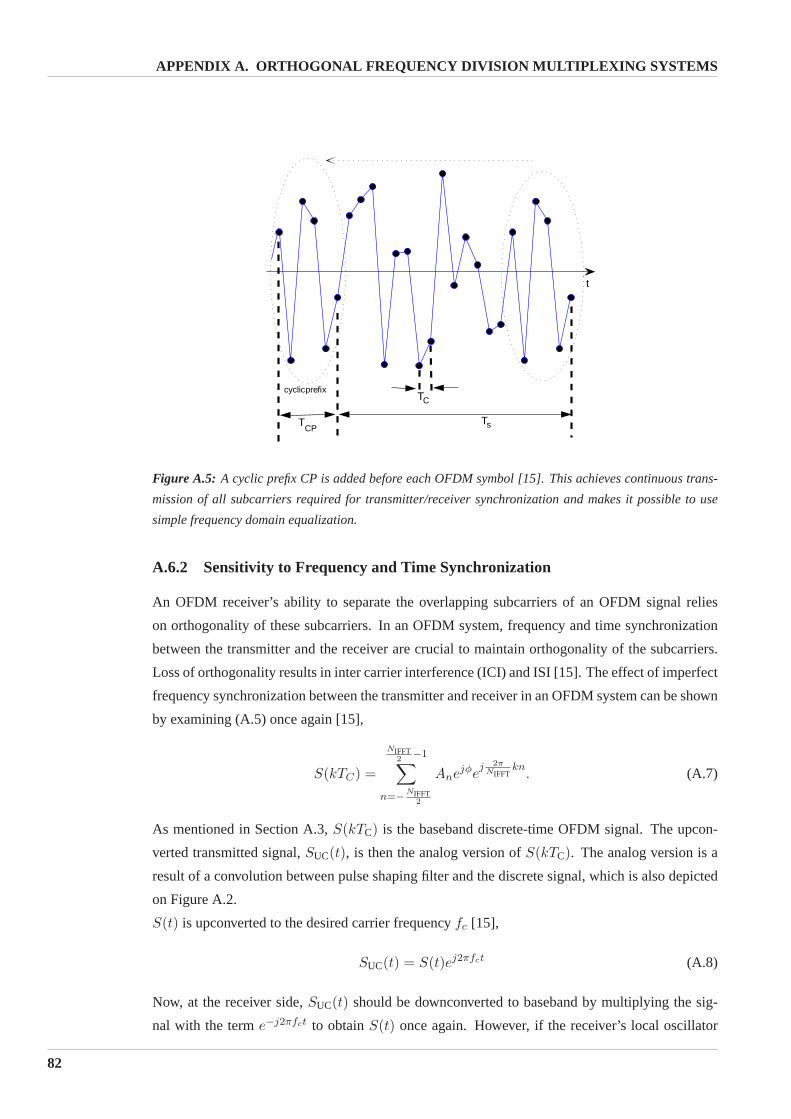
APPENDIX A. ORTHOGONAL FREQUENCY DIVISION MULTIPLEXING SYSTEMS
0 5 10 15 20 25 30−1.5
−1
−0.5
0
0.5
1
1.5
t
T
Ts
cyclic prefix
TCP
C
Figure A.5: A cyclic prefix CP is added before each OFDM symbol [15]. This achieves continuous trans-
mission of all subcarriers required for transmitter/receiver synchronization and makes it possible to use
simple frequency domain equalization.
A.6.2 Sensitivity to Frequency and Time Synchronization
An OFDM receiver’s ability to separate the overlapping subcarriers of an OFDM signal relies
on orthogonality of these subcarriers. In an OFDM system, frequency and time synchronization
between the transmitter and the receiver are crucial to maintain orthogonality of the subcarriers.
Loss of orthogonality results in inter carrier interference (ICI) and ISI[15]. The effect of imperfect
frequency synchronization between the transmitter and receiver in an OFDM system can be shown
by examining (A.5) once again [15],
S(kTC) =
NIFFT2
−1∑
n=−NIFFT2
Anejφej 2π
NIFFTkn
. (A.7)
As mentioned in Section A.3,S(kTC) is the baseband discrete-time OFDM signal. The upcon-
verted transmitted signal,SUC(t), is then the analog version ofS(kTC). The analog version is a
result of a convolution between pulse shaping filter and the discrete signal,which is also depicted
on Figure A.2.
S(t) is upconverted to the desired carrier frequencyfc [15],
SUC(t) = S(t)ej2πfct (A.8)
Now, at the receiver side,SUC(t) should be downconverted to baseband by multiplying the sig-
nal with the terme−j2πfct to obtainS(t) once again. However, if the receiver’s local oscillator
82

A.7. OFDM SIGNAL MODEL
frequency isfc + foff instead of being exactlyfc, the baseband signal received,Soffset(t), is then
Soffset(t) = SUC(t)e−j2π(fc+foff)t = S(t)e−j2fofft (A.9)
wherefoff is the receiver’s frequency error due to a frequency shift. The terme−j2fofft accounts
for ICI occurring due to the receiver’s frequency error. In otherwords, subcarriers no longer have
integer number of periods during an OFDM symbol period. Now, assuming aperfect matched
filtering and sampling frequency at the receiver,S(t) results in a discrete time signal,S(kTC), in
the form [15]
Soffset(kTC) = S(kTC)e−j2foffkTC =
NIFFT2
−1∑
n=−NIFFT2
Anejφne−j2foffkTCej 2π
NIFFTkn
(A.10)
The receiver’s FFT block then performs digital demodulation ofSoffset(kTC) to restore the trans-
mitted constellation points. In effect, this is equivalent to multiplyingS(kTC) with the term
ej 2π
NIFFTkn
. Therefore, when the distorted signalSoffset(kTC) is applied to the FFT block, the re-
ceived constellation points are [15]
Sc(k) =
NIFFT2
−1∑
n=−NIFFT2
Anejφne−j2foffkTC, (A.11)
whereSc(k) are the constellation points obtained at the output of the FFT block.
Hence, the effect of imperfect frequency synchronization is a phaserotation of constellation points
by an angleφerror = 2foffkTC. It can be seen thatφerr increases with both the frequency error and
time.
Loss of orthogonality can also result from loss of timing synchronization. At the receiver side, the
boundaries of OFDM symbols have to be located in order to apply the FFT window at the right
time.
Figure A.6: When there is a time shift, ISI occurs and hence received constellation points are distorted.
A.7 OFDM Signal Model
The properties of OFDM transmission has now been described. This section intends to describe
the OFDM transmission and the impact of the channel in mathematical terms followingthe same
83

APPENDIX A. ORTHOGONAL FREQUENCY DIVISION MULTIPLEXING SYSTEMS
structure as in [28, Sec. 2.3].
At the transmitter side, an OFDM symbol vectord[m] ∈ CNIFFT is mapped into a chip vectorµ[m]
at time indexm,
µ[m] = TCP1√
NIFFTF H
NIFFTd[m]. (A.12)
The discrete time has the rateTs and after parallel to serial conversion ofµ[m], the signal is
transmitted over a multipath channel.
TheNIFFT-point DFT-matrixFNIFFT ∈ CNIFFT×NIFFT with elements
[FNIFFT]i,l = e−j2πilNIFFT , i, l ∈ {0, 1, . . . NIFFT − 1} . (A.13)
The cyclic prefix is a result of matrixTCP,
TCP =
[0NIFFT−LCP
ICP
INIFFT
]∈ R
P×NIFFT. (A.14)
Matrix TCP copies the lastLCP chips of each OFDM symbol to the front.
If µ[n] denotes the chip sequence with rate1/Tc to be transmitted, then
µ[m] =
µ[mP ]...
µ[mP + P − 1]
∈ CP (A.15)
is the chip sequence sequence of one OFDM symbol.
Let us assume that the multipath channelh′[k] has an lengthL.
h′ =
h′[0]...
h′[L − 1]
∈ CL (A.16)
The received signal at the UE without noise is given by
x[n] =L∑
k=0
h[k]µ[n − k]. (A.17)
The received signalr is also affected by white Gaussian noisez[n] (N)(0, σ2z),
r[n] = x[n] + z[n]. (A.18)
The elementsx[n] andz[n] has the following structure for each OFDM symbol,
x[m] =
x[mP ]...
x[mP + P − 1]
∈ CP (A.19)
84

A.7. OFDM SIGNAL MODEL
and
z[m] =
z[mP ]...
z[mP + P − 1]
∈ CP . (A.20)
The influence of the channel is included by taking the lower and upper triangular Toeplitz channel
matrix into account.
H(0) =
h′[0] 0 0...
. .....
h′[L − 1]
0. ..
.... .. 0
0 . . . 0 h′[L − 1] . . . h′[0]
∈ CP×P (A.21)
and
H(1) =
0 . . . 0 h′[L − 1] . . . h′[1]. . . . .. . . .
...
h′[L − 1]
0 0...
...
0 . . . 0
∈ CP×P (A.22)
are the upper and lower triangular Toeplitz channel matrix respectively.
Now the intersymbol interference is modeled as,
x[m] = H(0)µ[m] + H(1)µ[m − 1], (A.23)
where the second term represents the inter-symbol interference between two consecutive OFDM
symbols, which affect the firstL samples ofx[m].
At the receiver the cyclic prefix of lengthLCP is removed by forming the product
RCPH(1) = 0NIFFT×P , where (A.24)
RCP = [0NIFFT×LCPINIFFT] ∈ R
NIFFT×P , (A.25)
with 0NIFFT×P and0NIFFT×LCPas matrices containing zeros with the dimensionsNIFFT × P and
NIFFT × LCP respectively. Equation (A.24) only holds if the maximum channel delayL − 1 is
less than or equal to the cyclic prefixLCP . The received signal is now written as,
y[m] = FRCP(x[m] + z[m]) = FRCPH(0)µ[m] + FRCPz
′[m]
= FRCPH(0)TCPF
HNIFFT
d[m] + FRCPz[m]
= F HF HNIFFT
d[m] + RCPz[m], (A.26)
85

APPENDIX A. ORTHOGONAL FREQUENCY DIVISION MULTIPLEXING SYSTEMS
where∈ CNIFFT×NIFFT is the overall circulant channel matrix and can be decomposed as,
H = RCPH(0)TCP = F H
NIFFTdiag(g)FNIFFT, (A.27)
whereg ∈ CNIFFT is defined as the DFT of the channel impulse responseh′,
g = FLh′, (A.28)
with FL as the truncated version ofF with the firstL columns.H(0) has a Toeplitz structure and
by inserting the cyclic prefix it is circularized. Hence the DFT-matrix are the eigenvectors, while
the channel matrix diag(g) is diagonal. Using Equation (A.26) and (A.27), the received signal can
be expressed as,
y[m] = diag(g)d[m] + z[m]. (A.29)
The elements of the noise vector,z[m] are white Gaussian with varianceσ2z and the covariance
matrix ofz[m] is diagonal with identical values
Rz[m] = E[FRCPz[m]z[m]HRH
CPFH]
(A.30)
= σ2zFRCPR
HCPF
H (A.31)
= σ2zINIFFT. (A.32)
From Equation (A.29), each symbol vectord[m] is transmitted over an individual frequency-flat
subcarrier.
A.8 Summary
Advances in DSPs have generated a great interest in OFDM as a spectrally efficient MCM scheme,
that is capable of delivering high data rates. The FFT is the basic algorithm inany OFDM sys-
tem, because it allows for a computationally efficient implementation. OFDM has high immunity
against frequency selective fading and ISI which makes it suitable for mobile communication.
OFDM transmission is also very sensitive to frequency and timing errors between the transmitter
and the receiver, which result in loss of orthogonality and therefore, ICI and ISI.
86

Generation of Reference Sym-
bolsB
B.1 Reference Symbol Sequences
The generation of reference symbols is based on [5].
As described in Section 2.4.2 the reference signal sequenceRref is generated as a symbol-by-
symbol product of an orthogonal sequenceROS ∈ C340×2 and a pseudo-random sequenceRPRS∈
R340×2. If rm,n is the entry atm’th row andn’th column ofRref, wherem = 0..339 andn = 0..1,
then
rm,n = rOSm,n · rPRS
m,n, (B.1)
There areNOS = 3 different orthognal sequences andNPRS = 170 different psudo-random se-
quences. The cells are divided into three identity groups at the physical layer level. There is a
one-to-one mapping between the three identities and the three two-dimensionalorthogonal se-
quences.
B.2 Orthogonal Symbol Sequences
The two-dimensional orthogonal sequence is generated as following:
rOSm,n = sm,n, (B.2)
wheresm,n is the entry at them’th row and then’th column of the matrixSi, defined as
STi =
STi , ST
i , . . . , STi︸ ︷︷ ︸
114 repetitions
, i = 0...2 (B.3)
where
ST1 =
1 1
1 1
1 1
ST1 =
1 ej4π/3
ej2π/3 1
ej4π/3 ej2π/3
ST1 =
1 ej2π/3
ej4π/3 1
ej2π/3 ej4π/3
(B.4)
APPENDIX B. GENERATION OF REFERENCE SYMBOLS
B.3 Pseudo-Random Sequences
The definition of the pseudo-random sequences in LTE is still in progressand has not yet been
determined. At present knowledge the pseudo-random sequences mayvary from slot to slot and
there exit 170 different sequences. In this project only one reference symbol is needed, hence it
chosen to generateRPRSas a random sequences of+1 and−1.
B.4 Mapping of Reference Symbols onto Resource Elements
The two-dimensional reference signal sequenceRref is mapped to complex-valued modulation
symbols(a(p)k,l (i)), wherek is the OFDM symbol position in one slot andl is the position of the
subcarrier, whilep andi are the antenna port and slot number respectively:
a(p)l,k (i) = rm′,n, (B.5)
where entry(m′, n) of the reference symbol sequence is found as follows
m = 0, 1, . . . , ⌊ NBW
NRBBW/2
⌋ − 1 (B.6)
m′ = m + 170 − ⌊NBW
NRB⌋ (B.7)
n =
{0 and1 if p = 0 or p = 1
0 if p = 2 or p = 3. (B.8)
The entry(l, k) of the reference symbol sequence is then calculated as following,
k = 6m + (v + fhop (⌊i/2⌋)) mod6 where (B.9)
l =
0 if n = 0 andp = 0 or p = 1 (1)
1 if n = 0 andp = 2 or p = 3 (2)
Nsym − 3 if n = 1 (3)
. (B.10)
B.4.1 Reference Symbol Mapping Example
In this example the number of transmitter antennas is 1 (p = 0), in order to make it as simple
as possible. Using transmission bandwidth of 2.5 MHz,NBW = 150 according to Table 2.1 and
NRB = 12 as explained in section . The number of OFDM symbols in one slotNsym = 6 and it is
chosen not to use frequency hopping.
The reference symbol to be transmitted is found in the following procedure:
- The index(m′, n) is calculated.
Sincep = 1, n = 0 andn = 1 (Equation (B.8)).
m = m = 0, 1, . . . , ⌊1506/2⌋ − 1 = 0, 1, . . . , 24 (Equation (B.6)).
m′ = m + 170 − ⌊NBWNRB
⌋ = 158, 159, . . . , 182 (Equation (B.7)).
88

B.4. MAPPING OF REFERENCE SYMBOLS ONTO RESOURCE ELEMENTS
- The entry(l, k) of the mapping positions are now found. Equation (B.10),1 and (B.10),2
are true, sincen = 0, 1 andp = 0. Firstly the values(k, l) for n = 0 is calculated.
For n=0,k = 6m+(v + fhop (⌊i/2⌋)) mod6 = 6m+(v mod6) = 0, 6, . . . , 144. For
n=0, l=1.
For n=1,k = 6m + (v mod6) = 6m + (3 mod) 6) = 3, 9, . . . , 147. For n=1,l = 3.
In this example there is a reference symbol on the first and fourth OFDM symbol in one slot.
There is always a spacing between the reference symbols of 6 subcarriers. The reference symbols
are placed with an offset of 4 subcarriers at the fourth OFDM symbol.
An illustration of the structure is depicted on Figure B.1.
Figure B.1: Example of the reference symbol structure for one slot with 6OFDM symbols using one
antenna. Note that only the used subcarriers are depicted.
89