Channel Flow Optimization for Product Allocation in Grocery Retail by

Abhijeet Singh

Bachelor of Technology, Mechanical Engineering, Indian Institute of Technology (BHU), 2014

and

Yixuan Fang

Bachelor of Arts, Supply Chain Management, Michigan State University, 2017

SUBMITTED TO THE PROGRAM IN SUPPLY CHAIN MANAGEMENT

IN PARTIAL FULFILLMENT OF THE REQUIREMENTS FOR THE DEGREE OF

MASTER OF APPLIED SCIENCE IN SUPPLY CHAIN MANAGEMENT AT THE

MASSACHUSETTS INSTITUTE OF TECHNOLOGY

June 2021

© 2021 Abhijeet Singh and Yixuan Fang. All rights reserved. The authors hereby grant to MIT permission to reproduce and to distribute publicly paper and electronic

copies of this capstone document in whole or in part in any medium now known or hereafter created.

Signature of Author: ____________________________________________________________________

Department of Supply Chain Management May 14, 2021

Signature of Author: ____________________________________________________________________

Department of Supply Chain Management May 14, 2021

Certified by: __________________________________________________________________________ Dr. Eva Ponce

Executive Director, MITx MicroMasters Program in Supply Chain Management Capstone Advisor

Accepted by: __________________________________________________________________________ Prof. Yossi Sheffi

Director, Center for Transportation and Logistics Elisha Gray II Professor of Engineering Systems Professor, Civil and Environmental Engineering

2

Channel Flow Optimization for Product Allocation in Grocery Retail

by

Abhijeet Singh

and

Yixuan Fang

Submitted to the Program in Supply Chain Management on May 14, 2021 in Partial Fulfillment of the

Requirements for the Degree of Master of Applied Science in Supply Chain Management

ABSTRACT

Supply chain networks in the retail industry have become increasingly complex, giving rise to challenges in product flow from distribution centers to fulfillment locations. Product allocation, in particular, has emerged as a critical challenge for grocery retail companies as it helps them determine the shipping location and the shipping type for every product in their portfolio. The sponsoring company for this project wants to validate their current product allocation model by determining whether the input values used for certain key factors in their algorithm are correct or not. Further, the company wants to identify whether any other factors need to be incorporated into the model. To address the problem statement, our project is focused on simulating the product allocation model with a range of different inputs and layering in relevant cost components. This helps us identify the least cost scenario and the corresponding values for the input factors. We recommend these values for running the model in the future. Using the recommended solution can result in ~12% savings in logistics cost.

Capstone Advisor: Dr. Eva Ponce Title: Executive Director, MITx MicroMasters Program in Supply Chain Management

3

ACKNOWLEDGEMENTS

We would like to thank the Center for Transportation and Logistics at the Massachusetts

Institute of Technology (MIT) for providing us with an opportunity to apply the academic

concepts learned as part of the Supply Chain Management program to a real-world problem.

We also thank our advisor, Dr. Eva Ponce, for her constant guidance and support throughout

our project. It was invaluable for us to have her consistent feedback to drive the project in the

right direction and learn from her industry expertise and insights.

We are immensely grateful to the sponsoring company for providing us with a project that

helped us learn about a key supply chain process in the industry and also gave us the

opportunity to work on a critical problem for the business. We thank the team for their

assistance in helping us understand the process, for timely sharing all the relevant data and for

collaborating with us to constructively address the problem at hand. Working with the sponsor

team on this project has been a significant part of our learning experience at MIT.

Last but not least, we are very grateful to Toby Gooley and Pamela Siska for their coaching,

feedback and advice on writing this report.

4

TABLE OF CONTENTS

1 INTRODUCTION ....................................................................................................................... 6

1.1 About the company ......................................................................................................... 6

1.2 Project Objective .............................................................................................................. 7

1.3 Problem Statement .......................................................................................................... 8

2 LITERATURE REVIEW ............................................................................................................... 9

2.1 Product Allocation in Grocery Retail ................................................................................ 9

2.2 Impact of online channel ............................................................................................... 13

3 DATA AND METHODOLOGY .................................................................................................. 15

3.1 Current Model ............................................................................................................... 15

3.2 Data ................................................................................................................................ 20

3.3 Methodology ................................................................................................................. 21

3.4 Cost Calculations ............................................................................................................ 24

4 RESULTS AND DISCUSSION .................................................................................................... 27

4.1 Cost sensitivity to individual parameters ....................................................................... 27

4.2 Cost sensitivity to all combinations of cutoffs ............................................................... 30

4.3 Cost aggregated by DC ................................................................................................... 34

4.4 Limitations ..................................................................................................................... 35

5 CONCLUSION ......................................................................................................................... 37

6 REFERENCES .......................................................................................................................... 39

5

LIST OF FIGURES

Figure 1: Types of retail logistics network ...................................................................................... 9

Figure 2: Part of the supply chain in focus in this report .............................................................. 10

Figure 3: Cost Drivers in the DC-Retail store subsystem .............................................................. 12

Figure 4: Alteryx Workflow ........................................................................................................... 16

Figure 5: Shipping DC Decision Tree ............................................................................................. 18

Figure 6: Add shipping DC in Alteryx ............................................................................................ 19

Figure 7: Cutoff constants used in Alteryx .................................................................................... 22

Figure 8: Cost vs ven% cutoff ....................................................................................................... 28

Figure 9: Cost vs against mvmt cutoff .......................................................................................... 29

Figure 10: Cost vs dos cutoff ........................................................................................................ 30

Figure 11: Cost for all simulated input combinations ................................................................... 31

LIST OF TABLES

Table 1: Ranking of cutoff combinations in ascending order of total variance from minimum cost

scenario. ..................................................................................................................................... 339

Table 2: Cost components across DCs as % of total shipping costs .............................................. 34

6

1 INTRODUCTION

1.1 About the company

Retail Business Services, LLC, is the services company of Ahold Delhaize, currently providing

services to well-known grocery brands in the USA. Ahold Delhaize is a leading grocery retail group

with a global presence across the US, Europe, and Indonesia. Its net sales for 2019 were reported

at USD 47.8B (€40.1B), with 54M customers served every week through nearly 7,000 stores

(Ahold Delhaize, 2020). The company's biggest market is the US, where they have a strong

presence on the East Coast with renowned brands such as Stop & Shop, Food Lion, Giant, and

Hannaford, among others. The company serves its customers through both offline brick-and-

mortar stores as well as the online channel.

The company's vision is to create the leading local food shopping experience. In line with this

vision, one of the key growth drivers for the company is to improve product availability and

freshness across all the channels to offer their customers a seamless omnichannel experience

(Ahold Delhaize, 2020). This strategic choice creates a more complex supply chain, one which

they plan to transition into a fully integrated, self-distribution model that can enable cost savings,

enhance vendor relationships, and improve product availability. Our project is focused on

improving product availability and resultant cost savings in the company's supply chain by

improving upon an existing product allocation algorithm.

Retail Business Services will henceforth be referred to as the sponsor company throughout the

capstone. The team members from the company involved in the project will be collectively

referred to as the sponsor team.

7

1.2 Project Objective

Grocery retail business has become increasingly competitive due to the ever-changing

consumer preferences and the constantly evolving technology adopted by new companies.

Against the backdrop of this competitive pressure, many grocery retail companies are now in

the process of evaluating their operations to identify opportunities for improvement. Within

operations, one of the most critical areas of focus has been logistics and shipping. This

emphasis on logistics is also supported by the fact that logistics have traditionally been one of

the biggest contributors to the overall operational costs for retail companies. Average logistics

costs in the retail sector are in fact higher than for manufacturing companies (Van der Vlist,

2007).

In a bid to gain a competitive advantage in logistics, retailers have continuously assumed more

control over the logistics operations for which suppliers had traditionally been responsible. This

in turn has introduced new variables and challenges in the physical flow structures of the

logistics network for these retailers. Despite these developments, comprehensive research in

the area of retail logistics networks remains lacking. Additionally, the advent of e-commerce

and online orders for grocery has only increased the market competition and exacerbated the

need for a better understanding of the supply chain complexities involved.

Therefore, the objective of undertaking this project is to first, research and understand the key

variables that characterize the physical flow of a product in the supply chain and second,

include other tactical variables that may have been missing from the process of planning the

flow. For the sponsor company, we also seek to analyze the cost impact of changing these

variables on different DCs in the network.

8

1.3 Problem Statement

Many retail companies today face the challenge of making the right products available on the

right shelves at the right time. This challenge can only be addressed by ensuring that the

physical flow of the products leading up to the shelf is effective and efficient. Two of the most

important variables that govern this flow are the shipping location and the shipment type for

every product.

In the context of the sponsor company and for this project, the shipping location is a

distribution center from where the product is supplied to retail stores whereas shipment type

refers to the unit size for transporting the product. Both these variables are discussed in greater

detail in sections 2.1 and 3.1. The sponsor company currently has a model that allocates a

location and a shipment type for every product. This is referred to as the 'Product Allocation'

process. Although the model has been in use at the company for a few years, scientific proof on

whether it is optimal or not has been missing. Further, the model also seems to be missing

important supply chain considerations that have an impact on the physical flow of the product.

Therefore, the problem statement posed by the sponsor company is to validate the existing

product allocation model by determining whether values used for key input variables are

correct and also identifying any other input variables that are currently missing. This is defined

in the form of research questions in section 3.3.

9

2 LITERATURE REVIEW

2.1 Product Allocation in Grocery Retail

Retail operations have undergone a transformation in the last couple of decades. There has been

a trend toward shifting away from direct store delivery by suppliers to shipping via dedicated

distribution centers (DCs) now. The trend is perhaps the most prominent in grocery retail and is

expected to only strengthen with time. As shown in Figure 1, the presence of distribution centers

gives rise to different types of network configurations (Kuhn & Sternbeck, 2013).

(Source: Kuhn, H., & Sternbeck, M. G. (2013). Integrative retail logistics: An exploratory study. Operations Management Research, 6(1), 2–18)

Figure 1: Types of retail logistics network

10

In such grocery retail distribution networks, which are designed with DCs as nodes and trans-

shipment points, a critical decision is the allocation of products. The product allocation decision

comprises of assigning a shipping DC and a shipping type for every product in the portfolio. This

essentially determines how the product will 'flow' through the distribution channel to the final

fulfillment location, in this case the retail stores. As depicted in Figure 2, this project focuses on

the part of the supply chain between distribution centers and the retail stores.

(Source: Kuhn, H., & Sternbeck, M. G. (2013). Integrative retail logistics: An exploratory study. Operations Management Research, 6(1), 2–18)

Product allocation is impacted by a variety of factors such as the DC location, the stores served,

storage capacity, picking and packing systems. Allocation is also impacted by factors related to

Figure 2: Part of the supply chain in focus in this report

11

the product, such as item dimensions, rate of sale, and vendor minimums. Additionally, as

mentioned by Caputo & Pelagagge (2006), due to the fierce market competition and rising service

level expectations, there is an added pressure on logistics systems to regularly re-evaluate the

design of warehousing operations.

Currently, at the sponsor company, the distribution centers are classified as: Breakpack DC and

Full Case DC. The Breakpack DC is mainly focused on piece picking operations and, to some

extent, Full Case picking as well. The Full Case DC, on the other hand, is primarily focused on Full

Case picking only. According to an analysis done by the sponsor team, there is a rising trend in

frequency and volume of orders managed via the Breakpack DC. This is because as more and

more options differentiated by flavors and packaging are made available to customers, the

variety of stock-keeping units (SKUs) has increased and the volume of orders per SKU has

decreased. This is also reinforced by Caputo & Pelagagge (2006), who state that the orders from

stores to the distribution centers have become smaller in order to meet a more fragmented

demand from customers. This in turn is critical to the warehouse operations, as the operational

efficiency has to be increased while the warehousing costs have to be reduced at the same time.

In addition to DC-related considerations, other aspects of the allocation process include in-store

operations, product consolidation by the supplier, nature of the product, etc.

Holzapfel et al. (2016) focus on the decision problem of allocation and provide an optimization

model that minimizes relevant costs subject to certain constraints. The relevant costs identified,

as shown in Figure 3, belong to one of the subsystems of the supply chain: (1) inbound

transportation (supplier–DC); (2) warehousing; (3) outbound transportation (DC–TP); and (4) in-

store operations. These subsystems are analyzed along with the associated cost drivers. Holzapfel

et al. finally propose an integrative planning algorithm that assigns products to DCs and also

determines delivery frequencies between supply points and specific DCs.

12

(Source: Holzapfel, A., Kuhn, H., & Sternbeck, M. (n.d.). Product allocation to different types

of distribution center in retail logistics networks | Elsevier Enhanced Reader)

While we seek to adopt certain elements of this model in our project, it is important to note the

differences. First, the network structures can vary greatly across companies. For our project, the

network structure used in existing research does not necessarily apply. Therefore, the model

needs to be adapted in accordance with the network design at the sponsor company. Second,

the research mentioned above does not consider factors related to the product, such as its size

and volume, its rate of sale (velocity), and in-store stocking of the products. All these factors are

currently relevant to product allocation done by the sponsor company. We discuss the same in

greater detail in the Methodology chapter.

The key challenge with the current product allocation process lies in determining whether the

cutoff constants used for certain parameters in the algorithm are correct or not. Through our

project, we seek to address this by adopting the relevant cost calculations as done by Holzapfel

et. al to the context of the sponsor company. Based on these cost figures, we then recommend

the best set of cutoff values to be used for the allocation.

Figure 3: Cost Drivers in the DC-Retail store subsystem

13

2.2 Impact of online channel

In the last decade, we have observed a considerable growth in the e-commerce retail market.

This trend has only been accelerated by the COVID-19 pandemic. To keep up with this growth

and compete in this rapidly changing industry, both online and brick-and-mortar retailers are

revisiting and revamping their operating models with an aim to improve their operations and

capabilities (Ma, 2017).

One of the challenges that many retailers face today is offering a seamless experience to their

customers across channels. Some companies are still managing their online and physical

networks as totally separate, while others are at different stages of leveraging omnichannel

retailing. Omnichannel refers to the integration of multiple channels (online and offline) to

interact with customers and fulfill their orders (Chopra, 2016).

The advent of grocery sales through online channels has led to traditional brick-and-mortar

retailers reviewing, redesigning and leveraging their existing logistics networks to stay

competitive. Logistics network designs are mostly determined by the point at which the case

packs would be split into customer units. While on the one hand, in non-food logistics, channel

integration is mostly seen as beneficial, on the other hand, in grocery retailing, this depends

heavily on product, market, and retailer specifics (Wollenburg et al., 2017).

Wollenburg et al. (2017) provide a qualitative analysis of different design options to serve as a

decision support for retailers developing logistics networks to serve customers across channels.

Three options are identified for network configurations:

(1) Fulfilling online orders via traditional brick-and-mortar logistics wherein stores are supplied

in large quantities and case packs by DCs and online orders are picked in store or are home-

delivered from the store

14

(2) Introducing a dedicated online DC where case packs are broken up and stored in customer

units for online orders only

(3) All orders are fulfilled from the same channel-integrated DC where picking happens in parallel

or sequentially across all channels

Further discussed in the research are differences in grocery and non-food logistics. Logistics

networks are, therefore, not only being planned based on parameters such as cost savings,

transportation distances or operations synergies but also by considering the product, customer,

and market characteristics (Piotrowicz and Cuthbertson, 2014; Teo and Shu, 2004).

The set of DCs under discussion, for which our model identifies the best combination of input

cutoff values, is dedicated purely to the sponsor company's brick-and-mortar stores. For online

orders, the company has a separate dedicated DC. However, our methodology can be easily

extended, without significant modifications, to this DC as well. Furthermore, the approach we

suggest to determine the best cutoff values is highly generalizable.

15

3 DATA AND METHODOLOGY

In this section, we describe the product allocation algorithm at the sponsor company in detail,

also referred to as the "Channel Tool." We then discuss the data available and the methodology

adopted to arrive at our recommendations.

The channel tool is essentially a combination of data transformation steps and logical

comparisons to determine the best fulfillment option for any given product. The tool considers a

variety of factors to determine how a particular product will flow through the channel to the end

location (e.g., brick-and-mortar store). Decisions are made based on the cutoff values/constants

used for these factors. Products exhibiting values above and below these cutoffs are allocated

differently based on a decision tree.

The main goal of our project is to identify the best set of cutoff values that should be used for

item-related attributes and sale velocity of an item, and add any new factors that warrant an

inclusion in the channel tool. The scope of the study is limited to two of the company's biggest

brands – Hannaford and Food Lion in the New England market.

3.1 Current Model

We start by first analyzing the current model, which is built on Alteryx — a popular ETL (Extract,

Transform and Load) software for analytics and data science. The workflow is organized into five

steps, as shown in Figure 4.

16

1. Set the shipping DC: Using the SKU-level store movement (sale) data as the starting point,

the shipping DC is set for all the products for both the brands (Hannaford and Food Lion)

based on whether the products are Full Case items or Breakpack items. Figure 5 shows part

of the decision-tree diagram used to set the shipping DC. This is then configured with data in

an Alteryx workflow, as partly shown in Figure 6.

2. Calculate the velocity factor: This workflow joins store movement data to the store count

data and calculates the average weekly movement per store. This calculated metric is then

compared to a pre-decided cutoff value for movement and the recommended ship type is

determined as being Full Case, Breakpack, or Inner.

3. Add vendor constraints: After determining the recommended ship type and the DC, the tool

compares whether a different future shipping DC is recommended than the one currently

being used. This data is then rolled up to vendor level and joined with other vendor

information. The dataset helps to find out the item count at a vendor level as well as the

future DCs. More importantly, the workflow adds in vendor minimum order quantity as a

check.

Figure 4: Alteryx Workflow

17

4. Calculate DOS (Days of Supply): Next, for a given order quantity, the tool calculates the

inventory cover and rolls it up to the vendor and DC levels. If the vendor minimum order

quantity (MOQ) is met for all channels, the movement is finalized as is. However, if the vendor

MOQ is not met, then the SKU mix and volume mix of the vendor is evaluated against pre-

decided cutoffs. If the mix is found to be significant, a final channel for the vendor and the

product is set as per the first step. Otherwise, the products are dropped from movement.

5. Add shipping method and compare DOS: As a final step, the order DOS is compared against

the DOS per order minimum at the shipping DC. If the order DOS is found to be lower, then

the movement is finalized as per the channel determined in the first step.

18

Figure 5: Shipping DC Decision Tree

19

Figure 6: Add shipping DC in Alteryx

20

3.2 Data

There are several datasets which are fed into the decision tool, Alteryx. The following datasets

were provided by the sponsor team for our analysis:

Dataset Summary Data Fields

Breakpack Item List Volumes of each item

supported from each DC

Shipping DC, Item Info, Quantities

Shipped in Cases and Units

Bracket MOQ for each DC from each

vendor

Vendor Info, DC Info, MOQ

Product Catalog Detailed info for each product

Shipping Type, Item Info, Weight &

Dimensions, Pallet Factor, Case

Size, Merchandise Group, Buying

Price, and Vendor Info

Dry Movement Each product's movement per

DC per week

Item Info, DC Info, Date, and

Movement Volumes

Store Count

Number of stores that received

a particular product from a

given DC per week

Item Info, DC Info, Date, Store

Count

Future DC Grid Potential shipping type change

by switching between DCs

Old DC Info, Shipping type, and New

DC Info

21

3.3 Methodology

Through our discussions with the sponsor team, two questions critical to our study emerged:

Question 1: Are the attribute and velocity factors used to determine Full Case ship vs. Breakpack

ship correct?

Question 2: Which other factors should be layered into the tool to improve supply chain

efficiencies?

For Question 1, the two approaches under consideration based on our literature review were

optimization and simulation. Through our discussion with the sponsor team, it was realized that

for optimization, defining the objective function would require a larger internal exercise for the

sponsor company in order to gather the relevant data on all the variables. This could only be

done over a longer time horizon beyond the duration of this project. We also developed the

understanding that it would be more beneficial to generate a range of outcomes for different

combinations of cutoff values for the sponsor team to evaluate and choose from, rather than a

single optimal solution. Therefore, simulation was the selected approach for the project.

Specifically, we simulated the channel tool on Alteryx and ran the workflow iteratively with

varying inputs to generate a range of outputs. The inputs varied were the cutoff values/constants

used for key decision-making factors, as shown in Figure 7.

22

Figure 7: Cutoff constants used in Alteryx

The parameters involved are explained as follows:

1. Breakpack and Inner cutoff: This corresponds to the impact that rate of sale of an item

has on the shipping type of a product. The rate of sale is measured as the number of units

sold per unit per week and is commonly referred to as "Movement" in retail parlance.

Henceforth, this will be referenced as movement ("mvmt"). The cutoff value used

currently, as shown in, Figure 7 is 0.25. This implies that products for which the movement

is lower than 0.25 will have Breakpack or Inner as their shipping type. Products for which

movement is higher than 0.25 will be shipped as Full Case.

2. Cube outlier min and max: This cutoff value is used to determine whether the volume of

a shipping unit of an item is an outlier. Items that have a bigger volume than the max or

smaller volume than the min are classified as outliers and are treated separately for

product allocation.

3. Weight outlier min and max: Similar to the above. Items that are heavier than the max or

lighter than the min are classified as outliers.

4. DOS cutoff: DOS stands for Days of Supply and the cutoff value used is 14. This is used to

evaluate how many days of the current rate of sale can be covered by the order placed

with a vendor. Generally, it is preferable to keep DOS at a lower value across industries,

as it is related to inventory holding and occupancy costs.

23

5. Ven % cutoff: Ven stands for Vendor and the cutoff value used is 0.749. This corresponds

to the percentage of a product that is sourced from a particular vendor. Higher values are

preferred, as it indicates that a higher proportion of the quantity is being sourced from a

single vendor, which enables volume consolidation.

From the above parameters, we decided to focus on mvmt, DOS and ven%. This is because

through our discussions with the sponsor team, it was concluded that the outlier cutoffs cannot

be used as a lever for change. Changing these cutoff values would result in the extreme-sized

items being allocated differently. Since the volume and weight of the item itself cannot be

changed to have it fit within the min-max range, these cutoff values were excluded from further

analysis. Items that are extremely big or extremely small will need to continue to be handled

differently.

For the three parameters of interest, mvmt, DOS, and ven%, we simulated the Alteryx workflow

several times by varying the cutoff values and generated as output the allocation decision for

each run. The parameter cutoffs were varied within the following ranges:

1. mvmt: 0.20 to 0.50

2. Ven%: 0.50 to 0.90

3. DOS: 7 and 14

The allocation decision output for each run was an Excel spreadsheet with the future shipping DC

and future shipping type for every SKU in the system, along with relevant product information

such as the vendor, item description and product category. The next step was to evaluate which

of these outputs was the best one. For this, we sought to address Question 2.

For Question 2, our exploratory discussions with the team helped us understand which factors

might warrant an inclusion in the model. Our hypothesis included labor requirements and cost

implications. This was also supported by the sponsor team, who emphasized that minimizing cost

remains the most compelling objective. We obtained the necessary data for logistics costs

24

(handling, occupancy, transportation) and received relevant information on labor costs. Using

both of these, we estimated the total cost associated with each of the above simulated outputs.

The best combination of cutoffs was then determined by evaluating which of them had the least

cost associated with it. Section 3.4 contains the details on calculating the different cost

components and estimating the total cost.

3.4 Cost Calculations

For each of the different cutoff combinations, we generated the product allocation output using

the Channel Tool on Alteryx. Using each of the outputs generated, we estimated the total cost

that would be incurred for each cutoff combination. It should be noted that no changes were

made to the allocation itself based on these costs.

The Total Cost for each of the simulated outputs was calculated as the sum of Handling,

Occupancy, Transportation, and Retail Stocking Costs. In order to calculate the different cost

components, we first estimate the number of cases shipped as well as the cubic volume of these

cases across all stores annually.

Annual Cases = Avg. Cases per store per week * 52 * Stores Served

Annual Cubes = Avg. Cases * 52 * Old cube * Vendor Pack

a. Handling Cost

This includes the cost of handling -- storage, picking, and preparing the products at the DC. It is

further divided by case and by cube. This is done to account for the number of cases handled as

well as the size of the cases handled. Cube refers to the cubic volume of each case. Larger-volume

cases understandably have a higher cost of handling.

25

Handling cost by case is the product of the number of cases handled annually and the handling

by case rate. Similarly, handling cost by cube is the product of the number of cubes handled

annually and the handling by cube rate. These rates were provided by the sponsor team for the

purposes of our calculation. However, any information pertaining to rates and costs, including in

the following sections as well, will remain undisclosed in this paper.

Annual Handling Cube Cost = Annual Cubes * Handling by cube rate

Annual Handling Case Cost = Annual Cases * Handling by case rate

b. Occupancy Cost

This refers to the cost of occupying space in the DC. The basis for calculation is the cubic volume,

as larger-sized units will occupy more space and will have a greater cost apportioned to them.

On average, every unit occupies space in the DC for a duration that equals the days of supply or

"dos." Therefore, this component is calculated as the product of the annual cubes handled, the

days of supply and the occupancy rate.

Annual Occupancy Cost = Annual Cubes * dos * Occupancy rate

c. Transportation Cost

This is calculated as the product of the number of cubes handled annually and the transportation

rate per cube.

Annual Transportation Cost per store = Annual Cubes * Transportation rate

e. Retail Stocking Cost

This is the labor cost entailed at retail stores to stock the shelves. This component was calculated

as the product of the number of hours worked and the cost of labor per hour. For the number of

hours worked, we use the number of minutes taken to stock each product for Full Case and for

Breakpack units. There is also a "Break Factor" applied to all times to account for the paid breaks

26

given to associates in an 8-hour shift. The average hourly rate (AHR) is the labor cost for an

associate at the store. As discussed in part a, the figures for each of these rates will remain

undisclosed in our paper and will be treated as confidential data.

Hours = Minutes Taken/60

Retail Stocking Cost = Hours * # of cases * Break Factor* AHR

27

4 RESULTS AND DISCUSSION

After computing all the cost components, we summed them up to find the total cost for each

scenario. We then analyzed the sensitivity of cost to individual parameters. This was done to

better understand the impact each parameter has by itself on the cost, and also to check whether

there was any parameter that was dominantly driving the cost. We then performed a similar

sensitivity analysis for cost against all possible combinations of different parameter cutoff values.

The following section discusses the results obtained.

4.1 Cost sensitivity to individual parameters

a. Against ven% cutoff

We varied the ven cutoff value from 0.50 to 0.90 while keeping the other two parameter

cutoffs constant at their default values i.e., mvmt = 0.25 and dos = 14.

As shown in Figure 8, there only seems to be variation in the cost when ven is in the range of

0.65 to 0.85. The exact cost figures will remain undisclosed. Therefore, the vertical axis is only

labeled with orders of magnitude of cost to indicate the extent of variation.

28

b. Against mvmt cutoff

We varied the mvmt cutoff value from 0.20 to 0.50 while keeping the other two parameter

cutoffs constant at their default values i.e., ven = 0.75 and dos = 14.

As discussed in Section 3.3, this cutoff value helps determine whether a product has enough

sales velocity to be shipped as Full Case or not. Products with mvmt value above the cutoff

are classified as Full Case, whereas the ones below are classified for Breakpack shipping. This

implies that as we increase the mvmt cutoff value, fewer products will meet the Full Case

criteria, and therefore the number of products which can be shipped as Full Case will decrease

and the number of Breakpack shipments will increase. More Breakpack shipments result in

higher transportation, occupancy and case handling costs. As can be seen in Figure 9, these

cost components increase notably. As discussed in part a, the exact cost figures remain

Figure 8: Cost vs ven% cutoff

x

2x

3x

4x

29

undisclosed. The vertical axis is only labeled with orders of magnitude of cost to indicate the

extent of variation.

Figure 9: Cost vs. against mvmt cutoff

c. Against dos cutoff

For the dos cutoff value, we only tested out two values, 7 and 14, while keeping the other

two parameter cutoffs constant at their default values i.e., ven = 0.75 and mvmt = 0.25. The

results are shown in Figure 10. It was decided that we would only test multiples of 7 for dos

as it is a common practice in the industry to measure supply in terms of the number of weeks

that the inventory can cover demand for. Additionally, increasing the cutoff to a higher

number (21) would not have been feasible for the sponsor company to act on. Higher days of

x

2x

3x

4x

30

supply would require increased warehouse capacity. This in turn, would have much larger

implications for the sponsor company which are beyond the scope of our project.

Figure 10: Cost vs. dos cutoff

4.2 Cost sensitivity to all combinations of cutoffs

Next, we plotted all the cost components as well as the total cost against all possible

combinations of the mvmt, ven%, and dos inputs. As shown in Figure 11, the total cost curve

follows a repeating (but not identical) pattern of decreasing most significantly against increasing

mvmt cutoff. Again, the vertical axis has been labeled with orders of magnitude of the cost so as

to keep the actual figures undisclosed.

x

1.5x

2x

0.5x

31

Figure 11: Cost for all simulated input combinations

x 2x

3x

4x

5x

32

We also ranked all the different simulations with dos = 14 in ascending order of total variance,

from the minimum cost scenario i.e., best case to worst case. This is shown in Table 1, where

total variance can be seen in the column titled "Total_Var%." The variances for each of the cost

components have also been tabulated (with a similar naming convention) to understand how

each of them varies with the cutoffs.

The first three rows in the table have the least variance (~ 5%), and represent that they are closest

to the least-cost scenario. This implies that these rows correspond to the best combinations of

cutoffs that should be used for product allocation. On the other hand, the bottom three rows,

with a total variance of up to 70%, represent that the corresponding combinations of cutoffs are

the farthest away from the least-cost scenario.

The sponsor company currently uses mvmt = 0.25, ven = 0.75 and dos = 14 as their default cutoffs

for product allocation. This particular combination corresponds to a total variance of 17.5%, as

can be seen from Table 1. Since the first three rows correspond to a variance of 5.4%, therefore,

it is possible for the team to reduce their total cost by about 12.1% calculated as the difference

of 17.5% and 5.4%. This can be achieved by simply changing the cutoffs to mvmt = 0.20, ven =

0.80 and dos = 14.

Although we also simulated the model for dos = 7 as well (the best-case scenario with 0% variance

in fact has dos = 7), we have not included those values in Table 1. This is because even though it

can lead to greater savings in costs, a reduction in days of supply in practice leads to much lower

inventory throughout the system. If undertaken, it will be a long-term strategic exercise for the

supply chain of the company. Recognizing this, for the purpose of our project, we therefore focus

on the results associated with dos = 14. From Table 1, it can be seen that mvmt = 0.2, ven = 0.70,

0.75 or 0.80 and dos = 14 are nearly identical. In fact, the total variance from the least cost

33

scenario is the same. Therefore, using any of these three sets of cutoffs as input settings to the

product allocation model is better than the default settings currently used.

Hence, our recommendation for cutoff values to be used for product allocation is mvmt = 0.2,

ven = 0.70, 0.75 or 0.80 and dos = 14. This can help reduce total cost by 12%, and can be

practically implemented in the short term.

Table 1: Ranking of input cutoff combinations in ascending order of total variance from minimum cost scenario

Inputs Total_Var%ven0.8mvmt0.2dos14 5.4ven0.75mvmt0.2dos14 5.4ven0.7mvmt0.2dos14 5.4ven0.8mvmt0.25dos14 17.5ven0.7mvmt0.25dos14 17.5ven0.75mvmt0.25dos14 17.5ven0.8mvmt0.3dos14 28.2ven0.75mvmt0.3dos14 28.2ven0.7mvmt0.35dos14 28.8ven0.7mvmt0.3dos14 28.8ven0.8mvmt0.35dos14 39.1ven0.75mvmt0.35dos14 40.6ven0.8mvmt0.4dos14 47.5ven0.7mvmt0.4dos14 50.6ven0.8mvmt0.45dos14 59.9ven0.75mvmt0.45dos14 60.6ven0.75mvmt0.4dos14 60.6ven0.7mvmt0.45dos14 61.9ven0.5mvmt0.25dos14 62.2ven0.85mvmt0.25dos14 62.2ven0.65mvmt0.25dos14 62.2ven0.6mvmt0.25dos14 62.2ven0.55mvmt0.25dos14 62.2ven0.9mvmt0.25dos14 62.2ven0.8mvmt0.5dos14 68.8ven0.75mvmt0.5dos14 70.7ven0.7mvmt0.5dos14 71.7

34

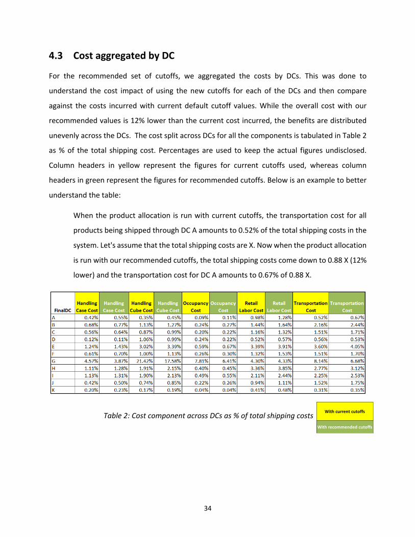
4.3 Cost aggregated by DC

For the recommended set of cutoffs, we aggregated the costs by DCs. This was done to

understand the cost impact of using the new cutoffs for each of the DCs and then compare

against the costs incurred with current default cutoff values. While the overall cost with our

recommended values is 12% lower than the current cost incurred, the benefits are distributed

unevenly across the DCs. The cost split across DCs for all the components is tabulated in Table 2

as % of the total shipping cost. Percentages are used to keep the actual figures undisclosed.

Column headers in yellow represent the figures for current cutoffs used, whereas column

headers in green represent the figures for recommended cutoffs. Below is an example to better

understand the table:

When the product allocation is run with current cutoffs, the transportation cost for all

products being shipped through DC A amounts to 0.52% of the total shipping costs in the

system. Let's assume that the total shipping costs are X. Now when the product allocation

is run with our recommended cutoffs, the total shipping costs come down to 0.88 X (12%

lower) and the transportation cost for DC A amounts to 0.67% of 0.88 X.

Table 2: Cost component across DCs as % of total shipping costs

With current cutoffs

With recommended cutoffs

35

4.4 Limitations

While our model comprehensively considers all relevant cost components to identify the least

cost scenario and recommend the corresponding cutoff values, there are some limitations to our

method of calculations which can be improved upon:

1. We varied the mvmt and ven cutoffs in increments of 0.05. For example, the range of testing

for mvmt was 0.20 to 0.50 and therefore, the values tested were 0.20, 0.25, 0.30, and so on.

This was done partly because these values were mathematically easier but also because of

computational limitations. Generating more outputs with smaller increments would have

resulted in many more combinations of cutoff values and subsequently many more outputs,

which would have been very difficult to handle in our tool for data analysis -- Python.

Further, during our initial analysis of sensitivity against individual parameters, we observed

that the output changes are unidirectional and largely linear. Therefore, the extreme values

of the output, which were of interest to us, would only occur at the lower and upper limits of

the input cutoff. In such a case, making smaller increments is not required as the

corresponding outputs will be irrelevant for practical purposes. However, when we test the

combination of cutoffs for all three of the parameters simultaneously to check the impact on

output, it may be possible to have the least cost correspond to a combination of cutoff values

that are not multiples of 0.05. Although this is a limitation for our model, we still expect our

recommended solution to be very close to the actual solution in this case. This can also be

inferred from Table 1, where we observe that the total variance % between two consecutive

cutoff increments is relatively low.

2. We carried out the simulation by manually running the Alteryx workflow repeatedly with

different combinations of cutoffs and generating the corresponding outputs. We then loaded

these outputs into Python for data analysis. This approach was time-consuming. An alternate

method would involve integrating Alteryx with Python and subsequently running the

36

workflow and recording the values directly within the Python environment. Not only would

this approach be faster, but it would also help eliminate any potential manual errors. This

requires an advanced understanding of integrating the two tools.

37

5 CONCLUSION

We started out the project by understanding product allocation and its evolving significance in

the grocery retail industry through literature review and discussions with the sponsor team and

our advisor. We then developed an in-depth understanding of product allocation within the

context of the sponsor company. After learning about the current model that the sponsor team

was using, familiarizing ourselves with Alteryx and obtaining the necessary data, we sought to

answer the following questions outlined in Section 3.3:

Question 1: Are the attribute and velocity factors used to determine Full Case ship vs. Breakpack

ship correct?

Question 2: Which other factors should be layered into the tool to improve supply chain

efficiencies?

To address these questions, we adopted the approach of simulation wherein we ran the Alteryx

workflow with a range of different input cutoffs that impacted product allocation decisions. In

particular, we focused on three key inputs – sale velocity of an item (mvmt), proportion of volume

sourced from a vendor (ven%) and days of supply (dos). We then analyzed the output scenarios

in Python by calculating the various relevant cost components for each output. The least-cost

scenario corresponds to our recommended cutoff values.

To be specific, the company currently uses mvmt = 0.25, ven = 0.75, dos = 14 as their cutoffs in

the workflow for product allocation. Based on our analysis, we identified that using mvmt = 0.20,

ven = 0.70, 0.75 or 0.80 and dos = 14 can result in cost savings of 12%. Further, this combination

of values was selected because it can be implemented without any impact on days of supply.

Days of supply is difficult to change and has larger implications for the supply chain of the

company, which are beyond the scope of this project. With our recommended combination of

cutoff values, we also analyzed the cost impact for every DC in the network to understand how

38

the various cost components would change across the DCs and found that the cost savings will

be unevenly distributed.

To conclude, we address the key research questions by first, identifying the optimal values for

attribute and velocity factors used to determine Full Case ship vs. Breakpack ship and second, by

including cost as an additional factor layered into the tool to help reduce the total cost incurred

in the system. The methodology is applicable to product allocation in general if the objective is

to reduce costs. Future research or projects on this topic could include building inventory

implications into the model. Reducing overall inventory in the system is another way of achieving

efficiencies in the supply chain. Additionally, the inventory capacity constraints at the DC could

also be factored in to ensure that the volume allocated to any DC can be accommodated there.

At a more strategic level, our project helps in developing an understanding of the key variables

that characterize the physical flow of a product in the supply chain and importantly, adds in a

new input variable for the sponsoring company. For supply chain managers in general, our study

helps highlight the importance of input parameter values used in product allocation and presents

an opportunity for improvement in cost efficiencies of the process.

39

6 REFERENCES

Ahold Delhaize Annual Report 2019. (2020).

https://www.aholddelhaize.com/media/10197/ahold-delhaize-annual-report-

2019.pdf

Bartholdi, J. And Steven, H. (2016). Warehouse & Distribution Science, Release 0.97.

Available at: www.warehouse-science.com.

Chopra, S. (2016). How omni-channel can be the future of retailing. Decision (0304-0941),

vol. 43(2), pp. 135-144. https://doi.org/10.1007/s40622-015-0118-9

Chopra, S. (2018). The evolution of omni-channel retailing and its impact on supply chains.

Transportation Research Procedia, vol. 30, pp. 4-13.

https://doi.org/10.1016/j.trpro.2018.09.002

Holzapfel, A., Kuhn, H., & Sternbeck, M. (n.d.). Product allocation to different types of

distribution center in retail logistics networks. Elsevier Enhanced Reader.

https://doi.org/10.1016/j.ejor.2016.09.013

Hubner, A., Kuhn, H., Sternbeck, M. (2010). Demand and supply chain planning in grocery

retail: an operations planning framework.

https://papers.ssrn.com/sol3/papers.cfm?abstract_id=1635752

Kuhn, H., & Sternbeck, M. G. (2013). Integrative retail logistics: An exploratory study.

Operations Management Research, 6(1), 2–18. https://doi.org/10.1007/s12063-012-

0075-9

40

Ma, S. (2017). Fast or free shipping options in online and omni-channel retail? The

mediating role of uncertainty on satisfaction and purchase intentions. International

Journal of Logistics Management, vol. 28(4), pp. 1099-1122.

https://doi.org/10.1108/IJLM-05-2016-0130

Richards, G. (2011). Warehouse Management. Kogan Page Limited.

The Future of Online Grocery. (2014). Oliver Wyman.

https://www.oliverwyman.com/content/dam/oliver-

wyman/global/en/2014/oct/OW_Future%20of%20Online%20Grocery_Final_ENG.pd

f

The metrics, they are a-changin'. (n.d.). Retrieved December 11, 2020, from

https://www.dcvelocity.com/articles/46914-the-metrics-they-are-a-changin

Wollenburg, J., Hubner, A., Kuhn, H., & Trautrims, A. (n.d.). From bricks-and-mortar to

bricks-and-clicks - ProQuest. Retrieved November 2, 2020, from

https://www.proquest.com/docview/2032697478/fulltextPDF/955F58DC04D14598

PQ/4?accountid=12492

Van der Vlist, P. (2007). Synchronizing the retail supply chain: synchroniseer de retail supply

chain, ERIM Ph.D. Series Research In Management, vol 110. Erasmus Research Inst.

of Management (ERIM), Rotterdam