Surpassing Human-Level Face Verification Performance on LFW withGaussianFace

Chaochao Lu Xiaoou TangDepartment of Information Engineering, The Chinese University of Hong Kong

{lc013, xtang}@ie.cuhk.edu.hk

Abstract

Face verification remains a challenging problem in verycomplex conditions with large variations such as pose,illumination, expression, and occlusions. This problemis exacerbated when we rely unrealistically on a singletraining data source, which is often insufficient to coverthe intrinsically complex face variations. This paper pro-poses a principled multi-task learning approach based onDiscriminative Gaussian Process Latent Variable Model,named GaussianFace, to enrich the diversity of trainingdata. In comparison to existing methods, our modelexploits additional data from multiple source-domains toimprove the generalization performance of face verificationin an unknown target-domain. Importantly, our modelcan adapt automatically to complex data distributions, andtherefore can well capture complex face variations inherentin multiple sources. Extensive experiments demonstratethe effectiveness of the proposed model in learning fromdiverse data sources and generalize to unseen domain.Specifically, the accuracy of our algorithm achieves animpressive accuracy rate of 98.52% on the well-known andchallenging Labeled Faces in the Wild (LFW) benchmark[23]. For the first time, the human-level performance inface verification (97.53%) [28] on LFW is surpassed. 1

1. IntroductionFace verification, which is the task of determining

whether a pair of face images are from the same person,has been an active research topic in computer vision fordecades [28, 22, 46, 5, 47, 31, 14, 9]. It has many importantapplications, including surveillance, access control, imageretrieval, and automatic log-on for personal computer ormobile devices. However, various visual complicationsdeteriorate the performance of face verification, as shownby numerous studies on real-world face images from thewild [23]. The Labeled Faces in the Wild (LFW) dataset

1For project update, please refer to mmlab.ie.cuhk.edu.hk.

is well known as a challenging benchmark for face ver-ification. The dataset provides a large set of relativelyunconstrained face images with complex variations in pose,lighting, expression, race, ethnicity, age, gender, clothing,hairstyles, and other parameters. Not surprisingly, LFWhas proven difficult for automatic face verification methods[23, 28]. Although there has been significant work [22, 9,5, 14, 47, 13, 59, 50, 51, 53] on LFW and the accuracyrate has been improved from 60.02% [56] to 97.35% [53]since LFW is established in 2007, these studies have notclosed the gap to human-level performance [28] in faceverification.

Why could not we surpass the human-level perfor-mance? Two possible reasons are found as follows:

1) Most existing face verification methods assume thatthe training data and the test data are drawn from thesame feature space and follow the same distribution. Whenthe distribution changes, these methods may suffer a largeperformance drop [58]. However, many practical scenariosinvolve cross-domain data drawn from different facialappearance distributions. Learning a model solely on asingle source data often leads to overfitting due to datasetbias [55]. Moreover, it is difficult to collect sufficientand necessary training data to rebuild the model in newscenarios, for highly accurate face verification specific tothe target domain. In such cases, it becomes critical toexploit more data from multiple source-domains to improvethe generalization of face verification methods in the target-domain.

2) Modern face verification methods are mainly dividedinto two categories: extracting low-level features [36, 3,34, 10, 24], and building classification models [62, 50,13, 37, 31, 56, 5, 28, 47, 33]. Although these existingmethods have made great progress in face verification, mostof them are less flexible when dealing with complex datadistributions. For the methods in the first category, forexample, low-level features such as SIFT [36], LBP [3],and Gabor [34] are handcrafted. Even for features learnedfrom data [10, 24], the algorithm parameters (such as thedepth of random projection tree, or the number of centers

1

arX

iv:1

404.

3840

v3 [

cs.C

V]

20

Dec

201

4

in k-means) also need to be specified by users. Similarly,for the methods in the second category, the architectures ofdeep networks in [62, 50, 63, 51] (for example, the numberof layers, the number of nodes in each layer, etc.), and theparameters of the models in [31, 5, 28, 47] (for example,the number of Gaussians, the number of classifiers, etc.)must also be determined in advance. Since most existingmethods require some assumptions to be made about thestructures of the data, they cannot work well when theassumptions are not valid. Moreover, due to the existence ofthe assumptions, it is hard to capture the intrinsic structuresof data using these methods.

To this end, we propose the Multi-Task Learning ap-proach based on Discriminative Gaussian Process LatentVariable Model (DGPLVM) [57], named GaussianFace, forface verification. Unlike most existing studies [22, 5, 14, 47,13] that rely on a single training data source, in order to takeadvantage of more data from multiple source-domains toimprove the performance in the target-domain, we introducethe multi-task learning constraint to DGPLVM. Here, weinvestigate the asymmetric multi-task learning because weonly focus on the performance improvement of the targettask. From the perspective of information theory, thisconstraint aims to maximize the mutual information be-tween the distributions of target-domain data and multiplesource-domains data. Moreover, the GaussianFace modelis a reformulation based on the Gaussian Processes (GPs)[42], which is a non-parametric Bayesian kernel method.Therefore, our model also can adapt its complexity flexiblyto the complex data distributions in the real-world, withoutany heuristics or manual tuning of parameters.

Reformulating GPs for large-scale multi-task learning isnon-trivial. To simplify calculations, we introduce a moreefficient equivalent form of Kernel Fisher DiscriminantAnalysis (KFDA) to DGPLVM. Despite that the Gaussian-Face model can be optimized effectively using the ScaledConjugate Gradient (SCG) technique, the inference is slowfor large-scale data. We make use of GP approximations[42] and anchor graphs [35] to speed up the process ofinference and prediction, so as to scale our model to large-scale data. Our model can be applied to face verification intwo different ways: as a binary classifier and as a featureextractor. In the former mode, given a pair of face images,we can directly compute the posterior likelihood for eachclass to make a prediction. In the latter mode, our model canautomatically extract high-dimensional features for eachpair of face images, and then feed them to a classifier tomake the final decision.

The main contributions of this paper are as follows:

• We propose a novel GaussianFace model for faceverification by virtue of the multi-task learning con-straint to DGPLVM. Our model can adapt to complexdistributions, avoid over-fitting, exploit discriminative

information, and take advantage of multiple source-domains data.

• We introduce a computationally more efficient equiva-lent form of KFDA to DGPLVM. This equivalent formreformulates KFDA to the kernel version consistentwith the covariance function in GPs, which greatlysimplifies calculations.

• We introduce approximation in GPs and anchor graphsto speed up the process of inference and prediction.

• We achieve superior performance on the challeng-ing LFW benchmark [23], with an accuracy rate of98.52%, beyond human-level performance reported in[28].

2. Related Work

Human and computer performance on face recognitionhas been compared extensively [40, 38, 2, 54, 41, 8]. Thesestudies have shown that computer-based algorithms weremore accurate than humans in well-controlled environ-ments (e.g., frontal view, natural expression, and controlledillumination), whilst still comparable to humans in thepoor condition (e.g., frontal view, natural expression, anduncontrolled illumination). However, the above conclusionis only verified on face datasets with controlled variations,where only one factor changes at a time [40, 38]. To date,there has been virtually no work showing that computer-based algorithms could surpass human performance onunconstrained face datasets, such as LFW, which exhibitsnatural (multifactor) variations in pose, lighting, expression,race, ethnicity, age, gender, clothing, hairstyles, and otherparameters.

There has been much work dealing with multifactorvariations in face verification. For example, Simonyanet al. applied the Fisher vector to face verification andachieved a good performance [47]. However, the Fishervector is derived from the Gaussian mixture model (GMM),where the number of Gaussians need to be specified byusers, which means it cannot cover complex data auto-matically. Li et al. proposed a non-parametric subspaceanalysis [33, 32], but it is only a linear transformationand cannot cover the complex distributions. Besides, therealso exist some approaches for utilizing plentiful source-domain data. Based on the Joint Bayesian algorithm [13],Cao et al. proposed a transfer learning approach [9] bymerging source-domain data with limited target-domaindata. Since this transfer learning approach is based onthe joint Bayesian model of original visual features, it isnot suitable for handling the complex nonlinear data andthe data with complex manifold structures. Moreover,the transfer learning approach in [9] only considered two

2

different domains, restricting its wider applications in large-scale data from multiple domains. More recently, Zhuet al. [63] learned the transformation from face imagesunder various poses and lighting conditions to a canonicalview with a deep convolutional network. Sun et al. [51]learned face representation with a deep model through faceidentification, which is a challenging multi-class predictiontask. Taigman et al. [52] first utilized explicit 3D facemodeling to apply a piecewise affine transformation, andthen derived a face representation from a nine-layer deepneural network. Although these methods have achievedhigh performances on LFW, many parameters of them mustbe determined in advance so that they are less flexible whendealing with complex data distributions.

The core of our algorithm is GPs. To the best of ourknowledge, GPs methods and Multi-task learning with re-lated GPs methods (MTGP) have not been applied for faceverification. Actually, MTGP/GPs have been extensivelystudied in machine learning and computer vision in recentyears [6, 60, 11, 25, 30, 44, 49, 61, 26]. However, mostof them [60, 11, 6, 44, 25, 49, 61] have only consideredthe symmetric multi-task learning, which means that alltasks have been assumed to be of equal importance, whereasour purpose is to enhance performance on a target taskgiven all other source tasks. Leen et al. proposed aMTGP model in the asymmetric setting [30] to focus onimproving performance on the target task, and Kim et al.developed a GP model for clustering [26], but their methodsdo not take the discriminative information of the covariancefunction into special account like DGPLVM. Although thediscriminative information is considered in [57], it doesnot apply multi-task learning to improve its performance.Salakhutdinov et al. used a deep belief net to learn a goodcovariance kernel for GPs [45]. The limitation of such deepmethods is that it is hard to determine which architecture forthis network is optimal. Also, multi-task learning constraintwas not considered in [45].

3. PreliminaryIn this section, we briefly review Gaussian Processes

(GPs) for classification and clustering [26], and GaussianProcess Latent Variable Model (GPLVM) [29]. We useGPs method mainly due to the following three notableadvantages. Firstly, as mentioned previously, it is a non-parametric method, which means it adapts its complexityflexibly to the complex data distributions in the real-world,without any heuristics or manual tuning of parameters.Secondly, GPs method can be computed effectively becauseof its closed-form marginal probability computation. Fur-thermore, its hyper-parameters can be learned from dataautomatically without using model selection methods suchas cross validation, thereby avoiding the high computationalcost. Thirdly, the inference of GPs is based on Bayesian

rules, resulting in robustness to overfitting. We recommendRasmussen and Williams’s excellent monograph for furtherreading [42].

3.1. Gaussian Processes for Binary Classification

Formally, for two-class classification, suppose that wehave a training setD ofN observations,D = {(xi, yi)}Ni=1,where the i-th input point xi ∈ RD and its correspondingoutput yi is binary, with y = 1i for one class and yi = −1for the other. Let X be the N × D matrix, where the rowvectors represent all n input points, and y be the columnvector of all n outputs. We define a latent variable fi foreach input point xi, and let f = [f1, . . . , fN ]>. A sigmoidfunction π(·) is imposed to squash the output of the latentfunction into [0, 1], π(fi) = p(yi = 1|fi). Assuming thedata set is i.i.d, then the joint likelihood factorizes to

p(y|f) =

N∏i=1

p(yi|fi) =

N∏i=1

π(yifi). (1)

Moreover, the posterior distribution over latent functions is

p(f |X,y,θ) =p(y|f)p(f |X)

p(y|X,θ). (2)

Since neither p(f |X,y,θ) nor p(y|f) can be computedanalytically, the Laplace method is utilized to approximatethe posterior

p(f |X,y,θ) = N (f , (K−1 + W)−1), (3)

where f = arg maxf p(f |X,y,θ) and W =−OO log p(f |X,y,θ)|f=f . Then, we can obtain

log p(y|X,θ) = −1

2f>K−1f + log p(y|f)− 1

2log |B|.

(4)

where |B| = |K| · |K−1 + W| = |In + W12 KW

12 |. The

optimal value of θ can be acquired by using the gradientmethod to maximize Equation (4). Given any unseen testpoint x∗, the probability of its latent function f∗ is

f∗|X,y, x∗ ∼ N (K∗K−1f ,K∗∗ −K∗K

−1K>∗ ), (5)

where K = K + W−1. Finally, we squash f∗ to find theprobability of class membership as follows

π(f∗) =

∫π(f∗)p(f∗|X,y, x∗)df∗. (6)

3.2. Gaussian Processes for Clustering

The principle of GP clustering is based on the key ob-servation that the variances of predictive values are smallerin dense areas and larger in sparse areas. The variancescan be employed as a good estimate of the support of a

3

probability density function, where each separate supportdomain can be considered as a cluster. This observation canbe explained from the variance function of any predictivedata point x∗

σ2(x∗) = K∗∗ −K∗K−1K>∗ . (7)

If x∗ is in a sparse region, then K∗K−1K>∗ becomes

small, which leads to large variance σ2(x∗), and vice versa.Another good property of Equation (7) is that it does notdepend on the labels, which means it can be applied to theunlabeled data.

To perform clustering, the following dynamic systemassociated with Equation (7) can be written as

F (x) = −Oσ2(x). (8)

The theorem in [26] guarantees that almost all the tra-jectories approach one of the stable equilibrium pointsdetected from Equation (8). After each data point findsits corresponding stable equilibrium point, we can employa complete graph [4, 26] to assign cluster labels to datapoints with the stable equilibrium points. Obviously, thevariance function in Equation (7) completely determines theperformance of clustering.

3.3. Gaussian Process Latent Variable Model

Let Z = [z1, . . . , zN ]> denote the matrix whose rowsrepresent corresponding positions of X in latent space,where zi ∈ Rd (d � D). The Gaussian Process LatentVariable Model (GPLVM) can be interpreted as a Gaussianprocess mapping from a low dimensional latent space to ahigh dimensional data set, where the locale of the pointsin latent space is determined by maximizing the Gaussianprocess likelihood with respect to Z. Given a covariancefunction for the Gaussian process, denoted by k(·, ·), thelikelihood of the data given the latent positions is as follows,

p(X|Z,θ) =1√

(2π)ND|K|Dexp

(− 1

2tr(K−1XX>)

),

(9)

where Ki,j = k(zi, zj). Therefore, the posterior can bewritten as

p(Z,θ|X) =1

Zap(X|Z,θ)p(Z)p(θ), (10)

where Za is a normalization constant, the uninformativepriors over θ, and the simple spherical Gaussian priors overZ are introduced [57]. To obtain the optimal θ and Z, weneed to optimize the above likelihood (10) with respect to θand Z, respectively.

4. GaussianFace

In order to automatically learn discriminative featuresor covariance function, and to take advantage of source-domain data to improve the performance in face verifi-cation, we develop a principled GaussianFace model byincluding the multi-task learning constraint into Discrimi-native Gaussian Process Latent Variable Model (DGPLVM)[57].

4.1. DGPLVM Reformulation

The DGPLVM is an extension of GPLVM, where the dis-criminative prior is placed over the latent positions, ratherthan a simple spherical Gaussian prior. The DGPLVM usesthe discriminative prior to encourage latent positions of thesame class to be close and those of different classes to be far.Since face verification is a binary classification problem andthe GPs mainly depend on the kernel function, it is naturalto use Kernel Fisher Discriminant Analysis (KFDA) [27]to model class structures in kernel spaces. For simplicity ofinference in the followings, we introduce another equivalentformulation of KFDA to replace the one in [57].

KFDA is a kernelized version of linear discriminantanalysis method. It finds the direction defined by a kernel ina feature space, onto which the projections of positive andnegative classes are well separated by maximizing the ratioof the between-class variance to the within-class variance.Formally, let {z1, . . . , zN+} denote the positive class and{zN++1, . . . , zN} the negative class, where the numbers ofpositive and negative classes are N+ and N− = N − N+,respectively. Let K be the kernel matrix. Therefore, inthe feature space, the two sets {φK(z1), . . . , φK(zN+

)} and{φK(zN++1), . . . , φK(zN )} represent the positive classand the negative class, respectively. The optimizationcriterion of KFDA is to maximize the ratio of the between-class variance to the within-class variance

J(ω,K) =(w>(µ+

K − µ−K))2

w>(Σ+K + Σ−K + λIN )w

, (11)

where λ is a positive regularization parameter, µ+K =

1N+

∑N+

i=1 φK(zi), µ−K = 1N−

∑Ni=N++1 φK(zi), Σ+

K =1N+

∑N+

i=1(φK(zi) − µ+K)(φK(zi) − µ+

K)>, and Σ−K =1N−

∑Ni=N++1(φK(zi)− µ−K)(φK(zi)− µ−K)>.

In this paper, however, we focus on the covariancefunction rather than the latent positions. To simplifycalculations, we represent Equation (11) with the kernelfunction, and let the kernel function have the same form asthe covariance function. Therefore, it is natural to introducea more efficient equivalent form of KFDA with certainassumptions as Kim et al. points out [27], i.e., maximizingEquation (11) is equivalent to maximizing the following

4

equation

J∗ =1

λ

(a>Ka− a>KA(λIn + AKA)−1AKa

), (12)

where

a =[1

n+1>N+

,− 1

N−1>N−

]

A =diag( 1√

N+

(IN+ −

1

N+1N+1>N+

),

1√N−

(IN− −

1

N−1N−1>N−

)).

Here, IN denotes theN×N identity matrix and 1N denotesthe length-N vector of all ones in RN .

Therefore, the discriminative prior over the latent posi-tions in DGPLVM can be written as

p(Z) =1

Zbexp

(− 1

σ2J∗), (13)

where Zb is a normalization constant, and σ2 represents aglobal scaling of the prior.

The covariance matrix obtained by DGPLVM is discrim-inative and more flexible than the one used in conventionalGPs for classification (GPC), since they are learned basedon a discriminative criterion, and more degrees of freedomare estimated than conventional kernel hyper-parameters.

4.2. Multi-task Learning Constraint

From an asymmetric multi-task learning perspective, thetasks should be allowed to share common hyper-parametersof the covariance function. Moreover, from an informationtheory perspective, the information cost between target taskand multiple source tasks should be minimized. A naturalway to quantify the information cost is to use the mutualentropy, because it is the measure of the mutual dependenceof two distributions. For multi-task learning, we extend themutual entropy to multiple distributions as follows

M = H(pt)−1

S

S∑i=1

H(pt|pi), (14)

whereH(·) is the marginal entropy,H(·|·) is the conditionalentropy, S is the number of source tasks, {pi}Si=1, and pt arethe probability distributions of source tasks and target task,respectively.

4.3. GaussianFace Model

In this section, we describe our GaussianFace modelin detail. Suppose we have S source-domain datasets{X1, . . . ,XS} and a target-domain data XT . For each

source-domain data or target-domain data Xi, according toEquation (9), we write its marginal likelihood

p(Xi|Zi,θ) =1√

(2π)ND|K|Dexp

(− 1

2tr(K−1XiX>i )

).

(15)

where Zi represents the domain-relevant latent space. Foreach source-domain data and target-domain data, theircovariance functions K have the same form because theyshare the same hyper-parameters θ. In this paper, we use awidely used kernel

Ki,j = kθ(zi, zj) =θ0 exp(− 1

2

d∑m=1

θm(zmi − zmj )2)

+ θd+1 +δzi,zj

θd+2, (16)

where θ = {θi}d+2i=0 and d is the dimension of the data

point. Then, from Equations (10), learning the DGPLVMis equivalent to optimizing

p(Zi,θ|Xi) =1

Zap(Xi|Zi,θ)p(Zi)p(θ), (17)

where p(Xi|Zi,θ) and p(Zi) are respectively representedin (15) and (13). According to the multi-task learningconstraint in Equation (14), we can attain

M =H(p(ZT ,θ|XT ))

− 1

S

S∑i=1

H(p(ZT ,θ|XT )|p(Zi,θ|Xi)). (18)

From Equations (15), (17), and (18), we know that learningthe GaussianFace model amounts to minimizing the follow-ing marginal likelihood

LModel = − log p(ZT ,θ|XT )− βM, (19)

where the parameter β balances the relative importancebetween the target-domain data and the multi-task learningconstraint.

4.4. Optimization

For the model optimization, we first expand Equation(19) to obtain the following equation (ignoring the constantitems)

LModel =− logPT + βPT logPT

+β

S

S∑i=1

(PT,i logPi − PT,i logPT,i

), (20)

where Pi = p(Zi,θ|Xi) and Pi,j means that its correspond-ing covariance function is computed on both Xi and Xj .

5

We can now optimize Equation (20) with respect to thehyper-parameters θ and the latent positions Zi by the ScaledConjugate Gradient (SCG) technique. Since we focus onthe covariance matrix in this paper, here we only presentthe derivations of hyper-parameters. It is easy to get

∂LModel

∂θj=(β(logPT + 1)− 1

PT

)∂PT∂θj

+β

S

S∑i=1

PT,iPi· ∂Pi∂θj

+β

S

S∑i=1

(logPi − logPT,i − 1)∂PT,i∂θj

.

The above equation depends on the form ∂Pi

∂θjas follows

(ignoring the constant items)

∂Pi∂θj

=Pi∂ logPi∂θj

≈Pi(∂ log p(Xi|Zi,θ)

∂θj+∂ log p(Zi)

∂θj+∂ log p(θ)

∂θj

).

The above three terms can be easily obtained (ignoring theconstant items) by

∂ log p(Xi|Zi,θ)

∂θj≈− D

2Tr(K−1 ∂K

∂θj

)+

1

2Tr(K−1XiX>i K−1 ∂K

∂θj

),

∂ log p(Zi)∂θj

≈− 1

σ2

∂J∗i∂θj

=− 1

λσ2

(a>

∂K

∂θja− a>

∂K

∂θjAa

+ a>KA∂K

∂θjAKa− a>KA

∂K

∂θja),

∂ log p(θ)

∂θj=

1

θj,

where A = A(λIn + AKA)−1A. Thus, the desiredderivatives have been obtained.

4.5. Speedup

In the GaussianFace model, we need to invert thelarge matrix when doing inference and prediction. Forlarge problems, both storing the matrix and solving theassociated linear systems are computationally prohibitive.In this paper, we use the anchor graphs method [35] tospeed up this process. To put it simply, we first select q(q � n) anchors to cover a cloud of n data points, andform an n × q matrix Q, where Qi,j = kθ(zi, zj). zi andzj are from n latent data points and q anchors, respectively.Then the original kernel matrix K can be approximated as

K ≈ QQ>. Using the Woodbury identity [21], computingthe n× n matrix QQ> can be transformed into computingthe q × q matrix Q>Q, which is more efficient.

Speedup on Inference When optimizing Equation (19),we need to invert the matrix (λIn + AKA). Duringinference, we take q k-means clustering centers as anchorsto form Q. Substituting K ≈ QQ> into (λIn + AKA),and then using the Woodbury identity, we get

(λIn + AKA)−1 ≈ (λIn + AQQ>A)−1

= λ−1In − λ−1AQ(λIq + Q>AAQ)−1Q>A.

Similarly, let K−1 ≈ (K + τI)−1 where τ a constant term,then we can get

K−1 ≈ (K + τI)−1 ≈ τ−1In − τ−1Q(τIq + Q>Q)−1Q>.

Speedup on Prediction When we compute the predic-tive variance σ(z∗), we need to invert the matrix (K +W−1). At this time, we can use the method in Section 3.2 tocalculate the accurate clustering centers that can be regardedas the anchors. Using the Woodbury identity again, weobtain

(K + W−1)−1 ≈W −WQ(Iq + Q>WQ)−1Q>W,

where (Iq +Q>WQ) is only a q×q matrix, and its inversematrix can be computed more efficiently.

5. GaussianFace Model for Face VerificationIn this section, we describe two applications of the

GaussianFace model to face verification: as a binaryclassifier and as a feature extractor.

Each face image is first normalized to 150 × 120 sizeby an affine transformation based on five landmarks (twoeyes, nose, and two mouth corners). The image is thendivided into overlapped patches of 25 × 25 pixels with astride of 2 pixels. Each patch within the image is mapped toa vector by a certain descriptor, and the vector is regardedas the feature of the patch, denoted by {xAp }Pp=1 where Pis the number of patches within the face image A. In thispaper, the multi-scale LBP feature of each patch is extracted[14]. The difference is that the multi-scale LBP descriptorsare extracted at the center of each patch instead of accuratelandmarks.

5.1. GaussianFace Model as a Binary Classifier

For classification, our model can be regarded as anapproach to learn a covariance function for GPC, as shownin Figure 1 (a). Here, for a pair of face images A and Bfrom the same (or different) person, let the similarity vectorxi = [s1, . . . , sp, . . . , sP ]> be the input data point of theGaussianFace model, where sp is the similarity of xAp and

6

xBp , and its corresponding output is yi = 1 (or −1). Withthe learned hyper-parameters of covariance function fromthe training data, given any un-seen pair of face images,we first compute its similarity vector x∗ using the abovemethod, then estimate its latent representation z∗ using thesame method in [57], and finally predict whether the pairis from the same person through Equation (6). In thispaper, we prescribe the sigmoid function π(·) to be thecumulative Gaussian distribution Φ(·), which can be solvedanalytically as π∗ = Φ

(f∗(z∗)√1+σ2(z∗)

), where σ2(z∗) =

K∗∗ −K∗K−1K>∗ and f∗(z∗) = K∗K

−1f from Equation(5) [42]. We call the method GaussianFace-BC.

5.2. GaussianFace Model as a Feature Extractor

As a feature extractor, our model can be regarded as anapproach to automatically extract facial features, shown inFigure 1 (b). Here, for a pair of face images A and B fromthe same (or different) person, we regard the joint featurevector xi = [(xAi )>, (xBi )>]> as the input data point ofthe GaussianFace model, and its corresponding output isyi = 1 (or −1). To enhance the robustness of our approach,the flipped form of xi is also included; for example,xi = [(xBi )>, (xAi )>]>. After the hyper-parameters ofcovariance function are learnt from the training data, wefirst estimate the latent representations of the training datausing the same method in [57], then can use the methodin Section 3.2 to group the latent data points into differentclusters automatically. Suppose that we finally obtain Cclusters. The centers of these clusters are denoted by{ci}Ci=1, the variances of these clusters by {Σ2

i }Ci=1, andtheir weights by {wi}Ci=1 where wi is the ratio of thenumber of latent data points from the i-th cluster to thenumber of all latent data points. Then we refer to eachci as the input of Equation (5), and we can obtain itscorresponding probability pi and variance σ2

i . In fact,{ci}Ci=1 can be regarded as a codebook generated by ourmodel.

For any un-seen pair of face images, we also firstcompute its joint feature vector x∗ for each pair of patches,and estimate its latent representation z∗. Then we computeits first-order and second-order statistics to the centers.Similarly, we regard z∗ as the input of Equation (5), and canalso obtain its corresponding probability p∗ and varianceσ2∗. The statistics and variance of z∗ are represented

as its high-dimensional facial features, denoted by z∗ =[∆1

1,∆21,∆

31,∆

41, . . . ,∆

1C ,∆

2C ,∆

3C ,∆

4C ]>, where ∆1

i =

wi

(z∗−ci

Σi

), ∆2

i = wi

(z∗−ci

Σi

)2

, ∆3i = log p∗(1−pi)

pi(1−p∗) ,

and ∆4i =

σ2∗σ2i

. We then concatenate all of the newhigh-dimensional features from each pair of patches toform the final new high-dimensional feature for the pairof face images. The new high-dimensional facial features

A

B

⋯

⋯

⋯

⋯

⋯⋯

𝑺𝟏

𝑺𝑷

⋯ GaussianFace Model As a Binary Classifier

SameOr

Different

Image pairMulti-scale

FeatureSimilarity

Vector

A

B

⋯

⋯

⋯

⋯⋯

⋯

GaussianFaceModel

As a Feature Extractor

Image pairMulti-scale

Feature

Joint Feature Vector and Its Flipped version

⋯ ⋯

⋯⋯

⋯ ⋯

⋯ ⋯

⋯

⋯

⋯

⋯

⋯

⋯

High-dimensional Feature

⋯

ConcatenatedFeature

(a)

(b)

Figure 1. Two approaches based on GaussianFace model for faceverification. (a) GaussianFace model as a binary classifier. (b)GaussianFace model as a feature extractor.

not only describe how the distribution of features of anun-seen face image differs from the distribution fitted tothe features of all training images, but also encode thepredictive information including the probabilities of labeland uncertainty. We call this approach GaussianFace-FE.

6. Experimental SettingsIn this section, we conduct experiments on face verifi-

cation. We start by introducing the source-domain datasetsand the target-domain dataset in all of our experiments (seeFigure 2 for examples). The source-domain datasets includefour different types of datasets as follows:Multi-PIE [19]. This dataset contains face images from337 subjects under 15 view points and 19 illuminationconditions in four recording sessions. These images arecollected under controlled conditions.MORPH [43]. The MORPH database contains 55,000images of more than 13,000 people within the age ranges of16 to 77. There are an average of 4 images per individual.Web Images2. This dataset contains around 40,000 facialimages from 3261 subjects; that is, approximately 10images for each person. The images were collected fromthe Web with significant variations in pose, expression, andillumination conditions.Life Photos2. This dataset contains approximately 5000images of 400 subjects collected online. Each subject hasroughly 10 images.

2These two datasets are collected by our own from the Web. It isguaranteed that these two datasets are mutually exclusive with the LFWdataset.

7

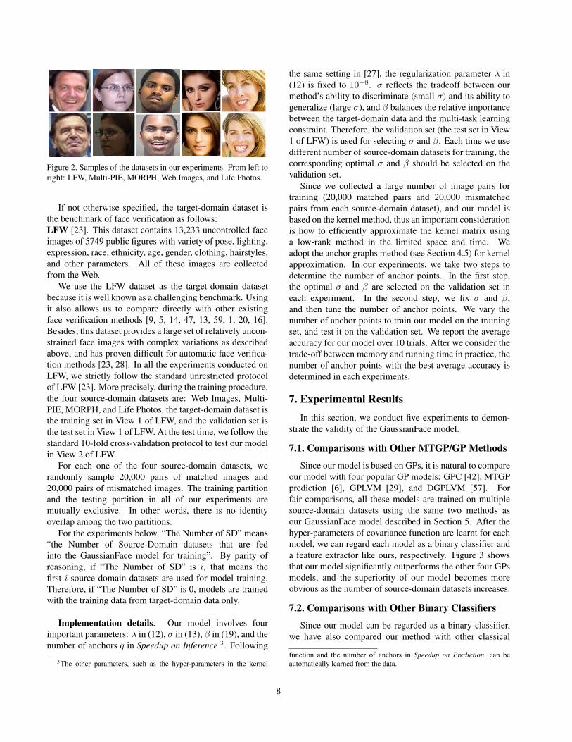
Figure 2. Samples of the datasets in our experiments. From left toright: LFW, Multi-PIE, MORPH, Web Images, and Life Photos.

If not otherwise specified, the target-domain dataset isthe benchmark of face verification as follows:LFW [23]. This dataset contains 13,233 uncontrolled faceimages of 5749 public figures with variety of pose, lighting,expression, race, ethnicity, age, gender, clothing, hairstyles,and other parameters. All of these images are collectedfrom the Web.

We use the LFW dataset as the target-domain datasetbecause it is well known as a challenging benchmark. Usingit also allows us to compare directly with other existingface verification methods [9, 5, 14, 47, 13, 59, 1, 20, 16].Besides, this dataset provides a large set of relatively uncon-strained face images with complex variations as describedabove, and has proven difficult for automatic face verifica-tion methods [23, 28]. In all the experiments conducted onLFW, we strictly follow the standard unrestricted protocolof LFW [23]. More precisely, during the training procedure,the four source-domain datasets are: Web Images, Multi-PIE, MORPH, and Life Photos, the target-domain dataset isthe training set in View 1 of LFW, and the validation set isthe test set in View 1 of LFW. At the test time, we follow thestandard 10-fold cross-validation protocol to test our modelin View 2 of LFW.

For each one of the four source-domain datasets, werandomly sample 20,000 pairs of matched images and20,000 pairs of mismatched images. The training partitionand the testing partition in all of our experiments aremutually exclusive. In other words, there is no identityoverlap among the two partitions.

For the experiments below, “The Number of SD” means“the Number of Source-Domain datasets that are fedinto the GaussianFace model for training”. By parity ofreasoning, if “The Number of SD” is i, that means thefirst i source-domain datasets are used for model training.Therefore, if “The Number of SD” is 0, models are trainedwith the training data from target-domain data only.

Implementation details. Our model involves fourimportant parameters: λ in (12), σ in (13), β in (19), and thenumber of anchors q in Speedup on Inference 3. Following

3The other parameters, such as the hyper-parameters in the kernel

the same setting in [27], the regularization parameter λ in(12) is fixed to 10−8. σ reflects the tradeoff between ourmethod’s ability to discriminate (small σ) and its ability togeneralize (large σ), and β balances the relative importancebetween the target-domain data and the multi-task learningconstraint. Therefore, the validation set (the test set in View1 of LFW) is used for selecting σ and β. Each time we usedifferent number of source-domain datasets for training, thecorresponding optimal σ and β should be selected on thevalidation set.

Since we collected a large number of image pairs fortraining (20,000 matched pairs and 20,000 mismatchedpairs from each source-domain dataset), and our model isbased on the kernel method, thus an important considerationis how to efficiently approximate the kernel matrix usinga low-rank method in the limited space and time. Weadopt the anchor graphs method (see Section 4.5) for kernelapproximation. In our experiments, we take two steps todetermine the number of anchor points. In the first step,the optimal σ and β are selected on the validation set ineach experiment. In the second step, we fix σ and β,and then tune the number of anchor points. We vary thenumber of anchor points to train our model on the trainingset, and test it on the validation set. We report the averageaccuracy for our model over 10 trials. After we consider thetrade-off between memory and running time in practice, thenumber of anchor points with the best average accuracy isdetermined in each experiments.

7. Experimental ResultsIn this section, we conduct five experiments to demon-

strate the validity of the GaussianFace model.

7.1. Comparisons with Other MTGP/GP Methods

Since our model is based on GPs, it is natural to compareour model with four popular GP models: GPC [42], MTGPprediction [6], GPLVM [29], and DGPLVM [57]. Forfair comparisons, all these models are trained on multiplesource-domain datasets using the same two methods asour GaussianFace model described in Section 5. After thehyper-parameters of covariance function are learnt for eachmodel, we can regard each model as a binary classifier anda feature extractor like ours, respectively. Figure 3 showsthat our model significantly outperforms the other four GPsmodels, and the superiority of our model becomes moreobvious as the number of source-domain datasets increases.

7.2. Comparisons with Other Binary Classifiers

Since our model can be regarded as a binary classifier,we have also compared our method with other classical

function and the number of anchors in Speedup on Prediction, can beautomatically learned from the data.

8

(a) (b)

0.740.760.78

0.80.820.840.860.88

0.90.920.940.96

0 1 2 3 4

Accu

racy

The Number of SD

GPC-BCMTGP prediction-BCGPLVM-BCDGPLVM-BCGaussianFace-BC

0.75

0.8

0.85

0.9

0.95

1

0 1 2 3 4

Accu

racy

The Number of SD

GPC-FEMTGP prediction-FEGPLVM-FEDGPLVM-FEGaussianFace-FE

0

0.01

0.02

0.03

0.04

0.05

0.06

0.07

0.08

0 1 2 3 4

Rela

tive

Impr

ovem

ent

The Number of SD

GPC-BCMTGP prediction-BCGPLVM-BCDGPLVM-BCGaussianFace-BC

0

0.01

0.02

0.03

0.04

0.05

0.06

0.07

0.08

0.09

0 1 2 3 4

Rela

tive

Impr

ovem

ent

The Number of SD

GPC-FEMTGP prediction-FEGPLVM-FEDGPLVM-FEGaussianFace-FE

(c) (d)

Figure 3. (a) The accuracy rate (%) of the GaussianFace-BC model and other competing MTGP/GP methods as a binary classifier. (b)The accuracy rate (%) of the GaussianFace-FE model and other competing MTGP/GP methods as a feature extractor. (c) The relativeimprovement of each method as a binary classifier with the increasing number of SD, compared to their performance when the numberof SD is 0. (d) The relative improvement of each method as a feature extractor with the increasing number of SD, compared to theirperformance when the number of SD is 0.

binary classifiers. For this paper, we chose three pop-ular representatives: SVM [12], logistic regression (LR)[17], and Adaboost [18]. Table 1 demonstrates that theperformance of our method GaussianFace-BC is muchbetter than those of the other classifiers. Furthermore,these experimental results demonstrates the effectivenessof the multi-task learning constraint. For example, ourGaussianFace-BC has about 7.5% improvement when allfour source-domain datasets are used for training, while thebest one of the other three binary classifiers has only around4% improvement.

7.3. Comparisons with Other Feature Extractors

Our model can also be regarded as a feature extractor,which is implemented by clustering to generate a code-book. Therefore, we evaluate our method by comparing

The Number of SD 0 1 2 3 4SVM [12] 83.21 84.32 85.06 86.43 87.31LR [17] 81.14 81.92 82.65 83.84 84.75

Adaboost [18] 82.91 83.62 84.80 86.30 87.21GaussianFace-BC 86.25 88.24 90.01 92.22 93.73

Table 1. The accuracy rate (%) of our methods as a binary classifierand other competing methods on LFW using the increasingnumber of source-domain datasets.

it with three popular clustering methods: K-means [24],Random Projection (RP) tree [15], and Gaussian MixtureModel (GMM) [47]. Since our method can determine thenumber of clusters automatically, for fair comparison, allthe other methods generate the same number of clusters asours. As shown in Table 2, our method GaussianFace-FE

9

The Number of SD 0 1 2 3 4K-means [24] 84.71 85.20 85.74 86.81 87.68RP Tree [15] 85.11 85.70 86.45 87.52 88.34GMM [47] 86.63 87.02 87.58 88.60 89.21

GaussianFace-FE 89.33 91.04 93.31 95.62 97.79

Table 2. The accuracy rate (%) of our methods as a feature ex-tractor and other competing methods on LFW using the increasingnumber of source-domain datasets.

0 0.05 0.1 0.15 0.20.8

0.82

0.84

0.86

0.88

0.9

0.92

0.94

0.96

0.98

1

Tom-vs-Pete + Attribute (93.30%) [5]High dimensional LBP (95.17%) [14]Fisher Vector Faces (93.03%) [47]combined Joint Bayesian (92.42%) [13]Associate-Predict (90.57%) [59]TL Joint Bayesian (96.33%) [9]VisionLabs (92.90%) [1]Aurora (93.24%) [20]Face++ (97.27%) [16]Human, cropped (97.53%) [28]DeepFace-ensemble (97.35%) [53]GaussianFace-FE + GaussianFace-BC (98.52%)

false positive rate

true

posi

tive

rate

Figure 4. The ROC curve on LFW. Our method achieves the bestperformance, beating human-level performance.

significantly outperforms all of the compared approaches,which verifies the effectiveness of our method as a featureextractor. The results have also proved that the multi-tasklearning constraint is effective. Each time one different typeof source-domain dataset is added for training, the perfor-mance can be improved significantly. Our GaussianFace-FEmodel achieves over 8% improvement when the number ofSD varies from 0 to 4, which is much higher than the ∼3%improvement of the other methods.

7.4. Comparison with the state-of-art Methods

Motivated by the appealing performance of bothGaussianFace-BC and GaussianFace-FE, we further com-bine them for face verification. Specifically, after facial fea-tures are extracted using GaussianFace-FE, GaussianFace-BC 4 is used to make the final decision. Figure 4 showsthe results of this combination compared with state-of-the-art methods [9, 5, 14, 47, 13, 53, 59, 1, 20, 16]. The bestpublished result on the LFW benchmark is 97.35%, whichis achieved by [53]. Our GaussianFace model can improvethe accuracy to 98.52%, which for the first time beats thehuman-level performance (97.53%, cropped) [28]. Figure5 presents some example pairs that were always incorrectly

4Here, the GaussianFace BC is trained with the extracted high-dimensional features using GaussianFace-FE.

Figure 5. The two rows present examples of matched andmismatched pairs respectively from LFW that were incorrectlyclassified by the GaussianFace model.

classified by our model. Obviously, even for humans, it isalso difficult to verify some of them. Here, we emphasizethat the centers of patches, instead of the accurate and densefacial landmarks like [9], are utilized to extract multi-scalefeatures in our method. This makes our method simpler andeasier to use.

7.5. Further Validations: Shuffling the Source-Target

To further prove the validity of our model, we alsoconsider to treat Multi-PIE and MORPH respectively asthe target-domain dataset and the others as the source-domain datasets. The target-domain dataset is split into twomutually exclusive parts: one consisting of 20,000 matchedpairs and 20,000 mismatched pairs is used for training, theother is used for test. In the test set, similar to the protocol ofLFW, we select 10 mutually exclusive subsets, where eachsubset consists of 300 matched pairs and 300 mismatchedpairs. The experimental results are presented in Figure6. Each time one dataset is added to the training set, theperformance can be improved, even though the types of dataare very different in the training set.

8. General DiscussionThere is an implicit belief among many psychologists

and computer scientists that human face verification abili-ties are currently beyond existing computer-based face ver-ification algorithms [39]. This belief, however, is supportedmore by anecdotal impression than by scientific evidence.By contrast, there have already been a number of paperscomparing human and computer-based face verificationperformance [2, 54, 40, 41, 38, 8]. It has been shown thatthe best current face verification algorithms perform betterthan humans in the good and moderate conditions. So, it isreally not that difficult to beat human performance in somespecific scenarios.

As pointed out by [38, 48], humans and computer-basedalgorithms have different strategies in face verification.

10

(a) (b)

0.86

0.88

0.9

0.92

0.94

0.96

0.98

1

0 1 2 3 4

Accu

racy

The Number of SD

GaussianFace-BCGaussianFace-FEGaussianFace-FE + GaussianFace-BC

0.78

0.8

0.82

0.84

0.86

0.88

0.9

0.92

0.94

0.96

0 1 2 3 4

Accu

racy

The Number of SD

GaussianFace-BCGaussianFace-FEGaussianFace-FE + GaussianFace-BC

Figure 6. (a) The accuracy rate (%) of the GaussianFace model on Multi-PIE. (b) The accuracy rate (%) of the GaussianFace model onMORPH.

Indeed, by contrast to performance with unfamiliar faces,human face verification abilities for familiar faces arerelatively robust to changes in viewing parameters suchas illumination and pose. For example, Bruce [7] foundhuman recognition memory for unfamiliar faces droppedsubstantially when there were changes in viewing param-eters. Besides, humans can take advantages of non-faceconfigurable information from the combination of the faceand body (e.g., neck, shoulders). It has also been examinedin [28], where the human performance drops from 99.20%(tested using the original LFW images) to 97.53% (testedusing the cropped LFW images). Hence, the experimentscomparing human and computer performance may not showhuman face verification skill at their best, because humanswere asked to match the cropped faces of people previouslyunfamiliar to them. To the contrary, those experimentscan fully show the performance of computer-based faceverification algorithms. First, the algorithms can exploitinformation from enough training images with variations inall viewing parameters to improve face verification perfor-mance, which is similar to information humans acquire indeveloping face verification skills and in becoming familiarwith individuals. Second, the algorithms might exploituseful, but subtle, image-based detailed information thatgive them a slight, but consistent, advantage over humans.

Therefore, surpassing the human-level performance mayonly be symbolically significant. In reality, a lot ofchallenges still lay ahead. To compete successfully withhumans, more factors such as the robustness to familiarfaces and the usage of non-face information, need to be con-sidered in developing future face verification algorithms.

9. Conclusion and Future Work

This paper presents a principled Multi-Task Learningapproach based on Discriminative Gaussian Process Latent

Variable Model, named GaussianFace, for face verificationby including a computationally more efficient equivalentform of KFDA and the multi-task learning constraint tothe DGPLVM model. We use Gaussian Processes approx-imation and anchor graphs to speed up the inference andprediction of our model. Based on the GaussianFace model,we propose two different approaches for face verification.Extensive experiments on challenging datasets validate theefficacy of our model. The GaussianFace model finallysurpassed human-level face verification accuracy, thanks toexploiting additional data from multiple source-domains toimprove the generalization performance of face verificationin the target-domain and adapting automatically to complexface variations.

Although several techniques such as the Laplace approx-imation and anchor graph are introduced to speed up theprocess of inference and prediction in our GaussianFacemodel, it still takes a long time to train our model forthe high performance. In addition, large memory is alsonecessary. Therefore, for specific application, one needs tobalance the three dimensions: memory, running time, andperformance. Generally speaking, higher performance re-quires more memory and more running time. In the future,the issue of running time can be further addressed by thedistributed parallel algorithm or the GPU implementationof large matrix inversion. To address the issue of memory,some online algorithms for training need to be developed.Another more intuitive method is to seek a more efficientsparse representation for the large covariance matrix.

Acknowledgements

We would like to thank Deli Zhao and Chen ChangeLoy for their insightful discussions. This work is partiallysupported by ”CUHK Computer Vision Cooperation” grantfrom Huawei, and by the General Research Fund sponsored

11

by the Research Grants Council of Hong Kong (ProjectNo.CUHK 416510 and 416312) and Guangdong InnovativeResearch Team Program (No.201001D0104648280).

References

[1] Visionlabs. In Website: http://www.visionlabs.ru/face-recognition.

[2] A. Adler and M. E. Schuckers. Comparing humanand automatic face recognition performance. IEEETransactions on Systems, Man, and Cybernetics, PartB: Cybernetics, 37(5):1248–1255, 2007.

[3] T. Ahonen, A. Hadid, and M. Pietikainen. Facedescription with local binary patterns: Application toface recognition. TPAMI, 28(12):2037–2041, 2006.

[4] A. Ben-Hur, D. Horn, H. T. Siegelmann, and V. Vap-nik. Support vector clustering. JMLR, 2, 2002.

[5] T. Berg and P. N. Belhumeur. Tom-vs-pete classifiersand identity-preserving alignment for face verifica-tion. In BMVC, volume 1, page 5, 2012.

[6] E. Bonilla, K. M. Chai, and C. Williams. Multi-taskgaussian process prediction. In NIPS, 2008.

[7] V. Bruce. Changing faces: Visual and non-visualcoding processes in face recognition. British Journalof Psychology, 73(1):105–116, 1982.

[8] V. Bruce, P. J. Hancock, and A. M. Burton. Com-parisons between human and computer recognition offaces. In Automatic Face and Gesture Recognition,pages 408–413, 1998.

[9] X. Cao, D. Wipf, F. Wen, and G. Duan. A practicaltransfer learning algorithm for face verification. InICCV. 2013.

[10] Z. Cao, Q. Yin, X. Tang, and J. Sun. Face recognitionwith learning-based descriptor. In CVPR, pages 2707–2714, 2010.

[11] K. M. Chai. Multi-task learning with gaussianprocesses. The University of Edinburgh, 2010.

[12] C.-C. Chang and C.-J. Lin. Libsvm: a library forsupport vector machines. ACM TIST, 2(3):27, 2011.

[13] D. Chen, X. Cao, L. Wang, F. Wen, and J. Sun.Bayesian face revisited: A joint formulation. InECCV, pages 566–579. 2012.

[14] D. Chen, X. Cao, F. Wen, and J. Sun. Blessingof dimensionality: High-dimensional feature and itsefficient compression for face verification. In CVPR.2013.

[15] S. Dasgupta and Y. Freund. Random projectiontrees for vector quantization. IEEE Transactions onInformation Theory, 55(7):3229–3242, 2009.

[16] H. Fan, Z. Cao, Y. Jiang, Q. Yin, and C. Doudou.Learning deep face representation. arXiv preprintarXiv:1403.2802, 2014.

[17] R.-E. Fan, K.-W. Chang, C.-J. Hsieh, X.-R. Wang,and C.-J. Lin. Liblinear: A library for large linearclassification. JMLR, 9:1871–1874, 2008.

[18] Y. Freund, R. Schapire, and N. Abe. A shortintroduction to boosting. Journal-Japanese SocietyFor Artificial Intelligence, 14(771-780):1612, 1999.

[19] R. Gross, I. Matthews, J. Cohn, T. Kanade, andS. Baker. Multi-pie. Image and Vision Computing,28(5):807–813, 2010.

[20] T. Heseltine, P. Szeptycki, J. Gomes, M. Ruiz, andP. Li. Aurora face recognition technical report:Evaluation of algorithm aurora-c-2014-1 on labeledfaces in the wild.

[21] N. J. Higham. Accuracy and Stability of NumbericalAlgorithms. Number 48. Siam, 1996.

[22] G. Huang, H. Lee, and E. Learned-Miller. Learninghierarchical representations for face verification withconvolutional deep belief networks. In CVPR, 2012.

[23] G. B. Huang, M. Ramesh, T. Berg, and E. Learned-Miller. Labeled faces in the wild: A databasefor studying face recognition in unconstrained en-vironments. Technical Report 07-49, University ofMassachusetts, Amherst, 2007.

[24] S. U. Hussain, T. Napoleon, F. Jurie, et al. Facerecognition using local quantized patterns. In BMVC,2012.

[25] H.-C. Kim, D. Kim, Z. Ghahramani, and S. Y. Bang.Appearance-based gender classification with gaussianprocesses. Pattern Recognition Letters, 27(6):618–626, 2006.

[26] H.-C. Kim and J. Lee. Clustering based on gaussianprocesses. Neural computation, 19(11), 2007.

[27] S.-J. Kim, A. Magnani, and S. Boyd. Optimal kernelselection in kernel fisher discriminant analysis. InICML, pages 465–472, 2006.

[28] N. Kumar, A. C. Berg, P. N. Belhumeur, and S. K.Nayar. Attribute and simile classifiers for face verifi-cation. In ICCV, pages 365–372, 2009.

[29] N. D. Lawrence. Gaussian process latent variablemodels for visualisation of high dimensional data. InNIPS, volume 2, page 5, 2003.

[30] G. Leen, J. Peltonen, and S. Kaski. Focused multi-task learning using gaussian processes. In MachineLearning and Knowledge Discovery in Databases,pages 310–325. 2011.

[31] H. Li, G. Hua, Z. Lin, J. Brandt, and J. Yang.Probabilistic elastic matching for pose variant faceverification. In CVPR. 2013.

12

[32] Z. Li, D. Lin, and X. Tang. Nonparametric discrimi-nant analysis for face recognition. TPAMI, 31(4):755–761, 2009.

[33] Z. Li, W. Liu, D. Lin, and X. Tang. Nonparametricsubspace analysis for face recognition. In CVPR,volume 2, pages 961–966, 2005.

[34] C. Liu and H. Wechsler. Gabor feature based classi-fication using the enhanced fisher linear discriminantmodel for face recognition. TIP, 2002.

[35] W. Liu, J. He, and S.-F. Chang. Large graphconstruction for scalable semi-supervised learning. InICML, pages 679–686, 2010.

[36] D. G. Lowe. Distinctive image features from scale-invariant keypoints. IJCV, 60(2):91–110, 2004.

[37] B. Moghaddam, T. Jebara, and A. Pentland. Bayesianface recognition. Pattern Recognition, 33(11):1771–1782, 2000.

[38] A. J. O’Toole, X. An, J. Dunlop, V. Natu, and P. J.Phillips. Comparing face recognition algorithms tohumans on challenging tasks. ACM Transactions onApplied Perception, 9(4):16, 2012.

[39] A. J. OToole, F. Jiang, D. Roark, and H. Abdi.Predicting human performance for face recognition.Face Processing: Advanced Methods and Models.Elsevier, Amsterdam, 2006.

[40] A. J. O’Toole, P. J. Phillips, F. Jiang, J. Ayyad,N. Penard, and H. Abdi. Face recognition algorithmssurpass humans matching faces over changes in illu-mination. TPAMI, 29(9):1642–1646, 2007.

[41] P. J. Phillips and A. J. O’Toole. Comparison of humanand computer performance across face recognitionexperiments. Image and Vision Computing, 32(1):74–85, 2014.

[42] C. E. Rasmussen and C. K. I. Williams. Gaussianprocesses for machine learning. 2006.

[43] K. Ricanek and T. Tesafaye. Morph: A longitudinalimage database of normal adult age-progression. InAutomatic Face and Gesture Recognition, pages 341–345, 2006.

[44] O. Rudovic, I. Patras, and M. Pantic. Coupledgaussian process regression for pose-invariant facialexpression recognition. In ECCV. 2010.

[45] R. Salakhutdinov and G. E. Hinton. Using deepbelief nets to learn covariance kernels for gaussianprocesses. In NIPS, 2007.

[46] H. J. Seo and P. Milanfar. Face verification using thelark representation. TIFS, 6(4):1275–1286, 2011.

[47] K. Simonyan, O. M. Parkhi, A. Vedaldi, and A. Zisser-man. Fisher vector faces in the wild. IJCV, 60(2):91–110, 2004.

[48] P. Sinha, B. Balas, Y. Ostrovsky, and R. Russell. Facerecognition by humans: 20 results all computer visionresearchers should know about. Department of Brainand Cognitive Sciences, MIT, Cambridge, MA, 2005.

[49] G. Skolidis and G. Sanguinetti. Bayesian multitaskclassification with gaussian process priors. IEEETransactions on Neural Networks, 22(12), 2011.

[50] Y. Sun, X. Wang, and X. Tang. Hybrid deep learningfor face verification. In ICCV. 2013.

[51] Y. Sun, X. Wang, and X. Tang. Deep learning facerepresentation from predicting 10,000 classes. InCVPR, 2014.

[52] Y. Taigman, L. Wolf, and T. Hassner. Multiple one-shots for utilizing class label information. In BMVC,pages 1–12, 2009.

[53] Y. Taigman, M. Yang, M. Ranzato, and L. Wolf. Deep-Face: Closing the Gap to Human-Level Performancein Face Verification. CVPR, 2014.

[54] X. Tang and X. Wang. Face sketch recognition.IEEE Transactions on Circuits and Systems for VideoTechnology, 14(1):50–57, 2004.

[55] A. Torralba and A. A. Efros. Unbiased look at datasetbias. In CVPR, pages 1521–1528, 2011.

[56] M. A. Turk and A. P. Pentland. Face recognition usingeigenfaces. In CVPR, pages 586–591, 1991.

[57] R. Urtasun and T. Darrell. Discriminative gaussianprocess latent variable model for classification. InICML, pages 927–934, 2007.

[58] J. Wright and G. Hua. Implicit elastic matching withrandom projections for pose-variant face recognition.In CVPR, pages 1502–1509, 2009.

[59] Q. Yin, X. Tang, and J. Sun. An associate-predictmodel for face recognition. In CVPR, pages 497–504,2011.

[60] K. Yu, V. Tresp, and A. Schwaighofer. Learninggaussian processes from multiple tasks. In ICML,pages 1012–1019, 2005.

[61] Y. Zhang and D.-Y. Yeung. Multi-task warpedgaussian process for personalized age estimation. InCVPR, pages 2622–2629, 2010.

[62] Z. Zhu, P. Luo, X. Wang, and X. Tang. Deep learningidentity preserving face space. In ICCV. 2013.

[63] Z. Zhu, P. Luo, X. Wang, and X. Tang. Recovercanonical-view faces in the wild with deep neuralnetworks. arXiv:1404.3543, 2014.

13