chaotic mixing analyses by distribution matrices

study these flows are overviewed in this paper.It is well known that even for laminar flow at verylow Reynolds numbers mixing can lead to com-plex flow patterns, and that the exposure of suchpatterns may be understood by imploring thetheory of dynamical systems [3]. The motion ofpassive particles in such a flow is described by theset of ordinary differential equations,

1˙ ( , )x u= x t

119Applied RheologyMay/June 2000

CHAOTIC MIXING ANALYSES BY DISTRIBUTION MATRICES

Patrick D. Anderson and Han E. H. Meijer

Materials Technology, Dutch Polymer Institute, Eindhoven University of TechnologyP. O. Box 513, 5600 MB Eindhoven, The Netherlands

Fax: x31.40.2447355E-mail: [email protected] and [email protected]

Received: 31.5.2000, Final version: 7.6.2000

ABSTRACTDistributive fluid mixing in laminar flows is studied using the concept of concentration distribution mapping matri-ces, which is based on the original ideas of Spencer & Wiley [1], describing the evolution of the composition of twofluids of identical viscosity with no interfacial tension. The flow domain is divided into cells, and large-scale variationsin composition are tracked by following the cell-average concentrations of one fluid using the mapping method ofKruijt et al. [2]. An overview of recent results is presented here where prototype two- and three-dimensional time-periodic mixing flows are considered. Efficiency of different mixing protocols are compared and for a particular ex-ample the (possible) influence of fluid rheology on mixing is studied. Moreover, an extension of the current methodincluding the microstructure of the mixture is illustrated. Although here the method is illustrated making use of thesesimple flows, more practical, industrial mixers like twin screw extruders can be studied using the same approach.

ZUSAMMENFASSUNGDie Vermischung von Flüssigkeiten in laminarer Strömung wird anhand der ”Concentration Distribution MappingMatrice“-Methode, basierend auf den Arbeiten von Spencer & Wiley, untersucht [1]. Durch diese Methode wird diezeitliche Entwicklung der Zusammensetzung zweier Flüssigkeiten gleicher Viskosität ohne Grenzflächenspannungbeschrieben. Hierfür wird der Strömungsbereich zunächst in Zellen unterteilt und anschließend wird die Veränderungder Zusammensetzung, durch das Verfolgen der zellengemittelten Konzentrationen eines der beiden Fluide mittelsder ”Mapping Method“ nach Kruijt et al., beobachtet [2]. Dieser Beitrag gibt ein Überblick über neuere Resultate zutypischen zwei- und dreidimensionalen, zeitperiodischen Mischungströmungen. Die Effizienz verschiedener Misch-methoden wird verglichen und für ein ausgewähltes Beispiel wird der (mögliche) Einfluss der rheologischen Eigen-schaften der Flüssigkeiten auf den Mischungsvorgang untersucht. Ausserdem wird eine Erweiterung der Methodevorgestellt, die die Mikrostruktur der Mischung miteinbezieht. Obwohl diese Methode hier an einfachen Strö-mungssituationen illustriert wird, kann sie auch zur Untersuchung von mehr anwendungsorientierten, industriellenMischern, wie dem Doppelwellenextruder verwendet werden.

RÉSUMÉLe mélange distributif de fluide dans les écoulements laminaires est étudié au moyen du concept de matrices detraçage de distributions de concentration, qui est basé sur les idées originales de Spencer & Wiley [1], décrivant l’évo-lution de la composition de deux fluides avec des viscosités identiques et sans tension interfaciale. Le domained’écoulement est divisé en cellules et les variations à grande échelle en composition sont suivies en estimant les con-centrations moyennes d’un des deux fluides à l’aide de la méthode de tracé de Kruijt et al. [2]. Une revue des résul-tats récents est ici présentée, où des écoulements de mélange prototypes à deux et trois dimensions et avec unedépendance temporelle périodique sont considérés. Les efficacités des différents protocoles de mélange sont com-parées et pour un exemple particulier, l’influence (éventuelle) de la rhéologie du fluide sur l’action de mélange estétudiée. De plus, une extension de la méthode, où la microstructure du mélange est incorporée, est présentée. Mal-gré le fait que nous donnions ici des exemples où la méthode est appliquée dans le cas d’écoulements simples, d’unpoint de vue plus pratique, des mélangeurs industriels, comme les extrudeurs à vis jumelles, peuvent être étudiés enutilisant une approche similaire.

© Appl. Rheol. 10, 3, 119-133 (2000)

Bilder 14.02.2001 9:34 Uhr Seite 119

1 INTRODUCTIONFluid mixing processes receive a considerable amount of recognition because of their import-ance in nature and industry. Although in many cases mixing is associated with turbulent fluid motions, mixing of very viscous fluids constitutes an important class of mixing occurrences. These are typical for polymer blending, compounding, food processing etc, and some new models to

DOI: 10.1515/arh-2000-0008

where x = (x, y, z) denotes the position vector andu the local Eulerian velocity. The amount ofstretching is often used to characterise the qual-ity of mixing:

2

where I and L are the present and initial lengthof a material filament, respectively [4]. The effi-ciency of stretching in a two-dimensional flowranges from 1/t where the flow is steady and thedomain is closed, to exponential for a hyperbolic,unbounded, chaotic, flow. In chaotic flows thereorientation prevents the material lines fromfull alignment with the streamlines, whichwould lead to linear stretching, and this generalphenomena is known as chaotic advection. It isrelatively straightforward to generate a flow thatcan generate chaos; a necessary condition is ingeneral the crossing of streamlines. For three-dimensional flows, the efficiency of stretchingcan even be exponential for steady flow.

Computational analysis is an important toolin the quantitative estimation of stretching inpractical mixers. Most flows are fully threedimensional and time-dependent and numericalmethods are required to obtain the velocity fieldand the resulting stretching. An example is theKenics static mixer, a spatially-periodic duct flow,studied by Avalosse [5] using a finite elementmethod. Hobbs and Muzzio [6] showed that thestretching distributions in the Kenics mixer areself-similar. Another example is the partitioned-pipe mixer [7] consisting of a rotating pipe parti-tioned with a sequence of orthogonally placesrectangular plates. The system is characterisedby a parameter B, the ratio of cross-sectionaltwist to axial stretching, and for b = 0 the flow isregular and becomes chaotic with increasingvalues of b. Meleshko et al. [8] demonstrated,using this system, the importance of an accuratevelocity field in studying chaotic mixing flows.

Modern tools of chaos theory – Poincaré sec-tions [4], periodic point analysis [9, 10], andstretching distributions [11, 25] – provide a deepunderstanding of the mechanisms that makechaotic mixing so effective, even though they donot give a direct description of the final mixture.The goal of this paper is to present an overviewof some recent results where mixing is studiedby using a more explicit approach based on the

original ideas of Spencer and Wiley [1]. Instead oftrying to understand all details of mixing, byusing abovementioned tools from chaos theory,we use the concept of concentration distributionmatrices to study the advection of fluid. Oncesuch a distribution matrix is constructed it is verysimple (fast) to study different mixing protocolsor the influence of initial conditions.

Although the method will be exemplifiedmaking use of relatively straightforward two-and three-dimensional time-periodic prototypeflows, see Figure 1, in our laboratory at presentalso more practical, industrial, efficient mixerslike 3D space-periodic static mixing devices, ase.g. the multiflux mixer, and 3D time- or spaceperiodic dynamic mixing devices, as e.g. the co-rotating, closely intermeshing, self-wiping twinscrew extruder, are being studied using the sameapproach. Results, that allow for fast optimis-ation processes, e.g. concerning screw design, falloutside of the scope of this paper and will be pre-sented elsewhere.

The following Section discusses someresults based on the application of ”classical“dynamical methods applied to a three-dimen-sional prototype flow. Results will show that it ispossible to analyse this type of flow, but that itis hard to make a quantitative comparisonbetween mixing protocols. In Sections 3 and 4 thesame flow is studied using a technique based ondistribution matrices and now actual compari-sons are more straightforward. Finally, in Section5 it is shown that microstructure of the mixturecan be added to the computations.

120 Applied RheologyMay/June 2000

-h

1

-1

0

B

T

h x

y

Br

Bu

Bd Fr

Fl

Fu

Fd

Bl

Figure 1:Geometries of the 2D

and 3D cavity. In the upper figure

during the first half of theperiod the top (back) wall is

moved from left to right,and in the

second half of the periodthe opposite (front) wallmoved from left to right.

This protocol is denoted asthe TB protocol.

The scheme of the flowdomain for the cubic cavity

and notation for possiblemotions of front and back

walls is denoted in the lowerfigure; see text for explanation of the

notation used.

Bilder 14.02.2001 9:34 Uhr Seite 120

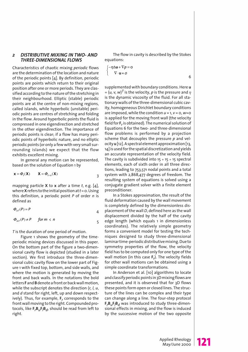
2 DISTRIBUTIVE MIXING IN TWO- ANDTHREE-DIMENSIONAL FLOWS

Characteristics of chaotic mixing periodic flowsare the determination of the location and natureof the periodic points [4]. By definition, periodicpoints are points which return to their originalposition after one or more periods. They are clas-sified according to the nature of the stretching intheir neighbourhood. Elliptic (stable) periodicpoints are at the centre of non-mixing regions,called islands, while hyperbolic (unstable) peri-odic points are centres of stretching and foldingin the flow. Around hyperbolic points the fluid iscompressed in one eigendirection and stretchedin the other eigendirection. The importance ofperiodic points is clear; if a flow has many peri-odic points of hyperbolic nature, and no ellipticperiodic points (or only a few with very small sur-rounding islands) we expect that the flowexhibits excellent mixing.

In general any motion can be represented,based on the solution of Equation 1 by

3

mapping particle X to x after a time t, e.g. [4],where X refers to the initial position at t = 0. Usingthis definition, a periodic point P of order n isdefined as

4

5

T is the duration of one period of motion.Figure 1 shows the geometry of the time-

periodic mixing devices discussed in this paper.On the bottom part of the figure a two-dimen-sional cavity flow is depicted (studied in a latersection). We first introduce the three-dimen-sional cubic cavity flow on the lower part of Fig-ure 1 with fixed top, bottom, and side walls, andwhere the motion is generated by moving thefront and back walls. In the notations the boldletters F and B denote a front or back wall motion,while the subscript denotes the direction (r, l, u,and d stand for right, left, up and down respect-ively). Thus, for example, Fr corresponds to thefront wall moving to the right. Compounded pro-tocols, like FrBuFlBd, should be read from left toright.

The flow in cavity is described by the Stokesequations:

6

supplemented with boundary conditions. Here u= (u, v, w)T is the velocity, p is the pressure and his the dynamic viscosity of the fluid. For all sta-tionary walls of the three-dimensional cubic cav-ity, homogeneous Dirichlet boundary conditionsare imposed, while the condition u = 1, v = 0, w=0is applied for the moving front wall (the velocityfield for Fr is obtained). The numerical solution ofEquations 6 for the two- and three-dimensionalflow problems is performed by a projectionscheme that decouples the pressure p and vel-ocity u [12]. A spectral element approximation [13,14] is used for the spatial discretization and yieldsan accurate representation of the velocity field.The cavity is subdivided into 15 * 15 * 15 spectralelements, each of sixth order in all three direc-tions, leading to 753,571 nodal points and a totalsystem with 2,868,477 degrees of freedom. Theresulting system of equations is solved using aconjugate gradient solver with a finite elementpreconditioner.

In a Stokes approximation, the result of thefluid deformation caused by the wall movementis completely defined by the dimensionless dis-placement of the wall D, defined here as the walldisplacement divided by the half of the cavityedge length (which equals 1 in dimensionlesscoordinates). The relatively simple geometryforms a convenient model for testing the tech-niques designed to study three-dimensionallaminar time-periodic distributive mixing. Due tosymmetry properties of the flow, the velocityfield has to be computed only for one type of thewall motion (in this case Fr). The velocity fieldsfor other wall motions can be obtained using asimple coordinate transformations.

In Anderson et al. [10] algorithms to locateand classify periodic points in 3D mixing flows arepresented, and it is observed that for 3D flowsthese points form open or closed lines. The struc-ture of the lines can be complex and their typecan change along a line. The four-step protocolFrBuFlBd was introduced to study three-dimen-sional effects in mixing, and the flow is inducedby the successive motion of the two opposite


Bilder 14.02.2001 10:20 Uhr Seite 121

walls in crossed directions as depicted in Figure 1.The net resulting displacement of each wall, afterone complete period, is zero.

The first-order periodic lines found are plot-ted in Figure 2. Hyperbolic parts of the line areplotted thin, elliptic lines are displayed thick. Forboth dimensionless displacement D-parametersthree periodic lines are found. In the first case,D = 3, two completely elliptic lines are revealedand one periodic line consisting of one ellipticpart and two hyperbolic tips. In the second case,D = 5, the periodic structure consists of three lineswith mixed types of periodic points. In Galak-tionov et al. [15] symmetry concepts of this floware discussed and rotational symmetry of theperiodic lines is proven.

The presence of hyperbolic periodic points inthe flow is important since it provides informa-tion of stretching. To emphasise the importanceof the periodic structure analysis, the motion oftwo blobs is calculated for a few periods. Anadaptive front tracking model is used to followthe deformation of the material volumes in anefficient way [16]. The initial sphere is coveredwith an unstructured triangular mesh consisting

of 258 nodes. The first blob is positioned aroundan elliptic point, the second one around a hyper-bolic point. The results for the case D = 5 are pre-sented in Figure 3. The difference in deformationbetween the two blobs is large and the blobaround the hyperbolic point is advected throughthe whole domain, while the stretching of theblob around the elliptic point is very small. Forthe blob around the elliptic part of the line, theinterfacial area remains nearly constant; how-ever, for the hyperbolic blob a substantialincrease in area is observed. 9689 nodes arerequired to describe the final deformation afterthree periods of flow. For both material blobs thevolume is preserved within a percent after threeperiods of mixing.

Using the definition of the deformation gra-dient FX = (—XFFT(X))T with FF as defined in Equa-tion 3 a useful definition of a stretching coeffi-cient at a periodic point can be defined:

7

where s(FX) is the eigenvalue spectrum of FX.Such an analysis is in particular of import-

ance when we are interested in the local behav-iour of periodic flows. The presence of low-orderhyperbolic periodic points is a clear indicationthat a mixing flow generates an exponentialincrease of interfacial area (albeit in a limitedpart of the flow domain). The stretching coeffi-cient at such a point is a measure for the rate ofmixing at the periodic point. If one has to favourone of the two mixing protocols, D = 3 or D = 5,the periodic point analysis may help to comparethese flows. However, guideness how to com-pare these protocols is unavailable. One mightcompare the arclength of the periodic lines con-sisting of hyperbolic points, and try to use thestretching coefficient at these points, but a sim-ple quantitative comparison based on the first-


Figure 2:Periodic lines in the

four-step 3D flow: thin – unstable

(hyperbolic) lines; thick – stable (elliptic) lines.

Upper plot for D = 3; lower plot for D = 5.

(Reproduced from Anderson et al.[10] with

permission of CambridgeUniversity Press).

Figure 3 a, b, c, d (fromf the two materialvolumes after one, two,

and th left to right): 3a shows two material

blob placed around ahyperbolic and an

elliptic periodic point forthe FrBuFlBd protocol

with D = 5. Sub-figures (b), (c),

and (d) show the deformation oree

periods, respectively.

S.122 14.02.2001 10:42 Uhr Seite 122

1

0

1 1

0

1

1

0

1

xy

z

1

0

1 1

0

1

1

0

1

xy

z

122/2 14.02.2001 10:50 Uhr Seite 122

Applied RheologyMay/June 2000

order results is still lacking. The maximumstretching coefficient equals 3.37 at the point(0.264, 0.469, 0.068) for the protocols D = 3, andfor the flow with D = 5 the coefficient equals 10.1at the point (–0.394, –0.458, 0.377). Based on thisinformation the higher dimensionless displace-ment seems to be favourable. A more extensivecomparison of protocols becomes a cumbersomerepetition and the need arises for a more flexiblemethod to distinguish a large numbers of mix-ing protocols, the topic of the remainder of thispaper.

3 MAPPING METHODThe ”mapping“ method is proposed based on theoriginal ideas of Spencer & Wiley [1], and themain idea is not to track each material volume inthe flow domain separately, but to create a dis-cretized mapping from a reference grid to adeformed grid. Instead of tracking the bound-aries of material volumes a set of distributionmatrices are used to advect concentration in theflow. Within the mapping method a flow domainΩ is subdivided into N non-overlapping sub-domains Ωi with boundaries ∂Wi, see Figure 4(top). The boundaries ∂Wi of these sub-domainsare represented by polygons and tracked from t= t0 to t = t0 + Dt using an adaptive front track-ing model [16], and, as a result, deformed poly-gons are obtained, see Figure 4 (bottom). Notethat the subdivision of Ω into Ωi’s is not relatedto any finite differences, or finite element dis-cretization used to solve the velocity field in Ω.Next, a discretized mapping from the initial gridto the deformed grid is constructed. The distrib-

ution of, for example, fluid concentration in theoriginal grid is then mapped to obtain a new dis-tribution.

The area of the intersections of the de-formed sub-domains with the original ones,determine the elements of the mapping (or dis-tribution) matrix y, where yij equals the fractionof the deformed sub-domain Wj at time t = t0 +∆t that is found in the original (t = t0) sub-domain Ωi

8The polygonal descriptions of the sub-domainsare used to determine the matrix elements yij,and the accuracy of these elements is deter-mined by the accuracy of the velocity field andthe error tolerances defined in the adaptive fronttracking procedure. For details on the validationand accuracy of the mapping method we refer toKruijt et al.[2]. The matrix y is essentially sparseif ∆t is not too large [2]. Where y will generallybe a sparse matrix, yn will generally be dense,since fluid from an initial subdomain will finallybe advected throughout the flow-domain. Thismakes studying the properties of yn, as original-ly proposed by Spencer and Wiley [1], both unat-tractive and even impossible for exponentialmixing flows. Therefore, instead of investigatingyn, e.g. C(n) could be investigated. C(n), the con-centration distribution after n mapping steps, iscomputed by the sequence for i = 1 to n

9

C(0) is the initial concentration distribution. Thisprocedure does not change the matrix y and is,therefore, much cheaper, both in number ofoperations as well as in the computer memoryneeded, than computing yn

The computation of the matrix elements yijis time consuming ; more than 100 hours using a12 CPU multiprocessor 225 Mhz R10K SiliconGraphics™ for a 200 * 120 grid. However, once thematrices are obtained matrix–vector multiplica-tions are extremly fast, less than 1 sec on a singleCPU 100 Mhz Pentium™, and a large number ofmixing protocols are easily compared.To differ-entiate between the quality of mixing protocols,mixing measures are applied.


Figure 4 (upper): Initial sub-domain discretization 10 * 6 grid;and deformed grid (below)after displacement of thetop wall by two times itslength. During the actual computations a finer 200 * 120 was used.

AR 3 14.02.2001 10:24 Uhr Seite 123

Here, the intensity of segregation I is used,which is a property of the mixture that is effect-ed by molecular diffusion. The intensity of seg-regation is a second-moment statistic (variance)of the concentration distribution and is definedas [17]:

10

where sc2 is the variance in concentration overan entire domain Ω, defined as:

11

and c(x) is the concentration in a point x Œ W inthe domain. The brackets < >Ω denote an aver-aging over the quantity in the brackets in Ω.Intensity of segregation is a measure of the devi-ation of the local concentration from the idealsituation (i.e. when the mixture is homo-geneous). A value of I equal to zero means nointensity, where a value of unity means a maxi-mum intensity (only black and white fluids andno gray fluid).

3.1 2D MAPPING METHOD

To demonstrate the strength of the mappingmethod, we first consider the two-dimensionalcavity flow as depicted in Figure 1 (top). The map-ping method is a flexible tool for studying andoptimising of mixing processes, since it makes itpossible to incorporate variations on an existingmixing protocol without having to recomputethe entire protocol. As a first illustration, twoparameters of the cavity flow are varied: thedimensionless displacement D and the numberof wall movements n; the product of which is pro-portional to energy input. Different protocols arecompared by changing the order of consecutivemappings.

Four different protocols are investigated. Inprotocol TTTT only the top wall moves, avoidingperiodicity in the flow, and a linear mixing flowresults. In protocol TBTB the top wall (T) and bot-tom wall (B) move alternatingly, in the directionsas depicted in Figure 1 (originally proposed byFranjione et al. [18]). Protocols TBTBBTBT and TB-T-B are variations on the second protocol pro-posed [4, 19, 20] to reduce the regularity of theprotocol, thus decreasing the size of regions


0 10 20 30 40 50 6010

5

104

103

102

101

100

Number of wall displacements

Inte

nsity

of s

egre

gatio

n

D = 5

TTTT TBTB TBTBBTBTTBTB

0 10 20 30 40 50 6010

5

104

103

102

101

100


Inte

nsity

of s

egre

gatio

n

D = 7


0 10 20 30 40 50 6010

5

104

103

102

101

100


Inte

nsity

of s

egre

gatio

n

D = 9


0 10 20 30 40 50 6010

5

104

103

102

101

100


Inte

nsity

of s

egre

gatio

n

D = 12


Figure 5:Comparison of different

mixing protocols.

Bilder 14.02.2001 10:11 Uhr Seite 124

around elliptic points (symmetry breaking pro-tocols). The minus-signs in the last protocoldenote a negative wall movement direction.

For these four protocols the concentrationdistribution is studied using the mapping matri-ces: yD=0.25, yD=1, yD=2 and yD=4 which are con-structed for the first protocol TTTT (consideringa movement of the top wall only). Combinationsof these mapping matrices are used to obtaindeformations for larger displacements. Forexample, to obtain the concentration distribu-tion after 7.5 wall displacements the matrix multi-plications yD=4yD=2yD=1yD=0.25yD=0.25C(0) areapplied. Since the geometry is symmetric (withthe origin in the centre of the cavity), the map fora movement of the bottom wall is the same as

for the top wall, but rotated (x and y values mul-tiplied by –1 in the coordinate system). Wallmovement in the opposite direction and move-ment of the opposite wall, can be computed bymirroring (multiplying the x and/or y-coordinateby –1 in the coordinate system of Figure 1), re-ducing the number of required matrices. For themapping calculations, a grid of 120 * 200 rec-tangular cells covers the interior of the cavity,and extends from –0.995h < x < 0.995h and–0.999 < y < 0.999, leaving a single, very thin cellaround the boundary. This boundary cell reducescomputational expenses, by avoiding the neces-sity to track points that pass very close to the cor-ner singularities.


Figure 6: Concentration distributions for the TB-T-B protocol with D = 9. Initially, the left half of thecavity is filled with whitefluid and the right half withblack fluid. After alreadyfour periods the fluids arereasonable mixed except fora relatively large zone in thecore of the flow. The fluid inthis weak zone is only slowly interchanged withthe fluid outside this zone.

t=1T t=2T

t=6Tt=4T

t=9Tt=8T

t=10T t=15T

Bilder 14.02.2001 10:11 Uhr Seite 125

The four protocols are compared and resultsfor four different dimensionless displacementare presented, i.e. D=5, 7, 9, and 12. Figure 5 showsthe decrease in intensity of segregation versusthe number of wall displacements for each proto-col. Except for the protocol with D = 7 it isobserved that the linear flow TTTT performsworst. From earlier studies [13, 4] it is known thatthe protocol TBTB has a large island for D approxi-mately between 5 and 7. The fluid within theisland is isolated and cannot reach the chaoticmixing zone. As a result the intensity of segre-gation remains about 10-1 for D = 7. The other pro-tocols provide better mixing and a faster rate atwhich these protocol reach the minimum level ofintensity of segregation (a noise level resultingfrom small numerical errors). For most systemsin Figure 5 it is noted that after some initial tran-sient effects a constant decrease of intensity ofsegregation is observed until the minimum levelis reached. Except for the TB-T-B protocol withD = 9 and we examine this system in more detailin Figure 6.

It shows the fluid concentrations after someinteger number of periods. After one period offlow many striations are already observed, butalso large areas of white and black fluid are seen.A weak zone appears to be present in this flowwhich only slowly interchanges fluid outside thiszone, explaining the behaviour of the intensityof segregation as observed in Figure 5.

Figure 7 shows some effects of the rheologyof the fluid on mixing. Here the Carreau model isused with zero infinite-shear-rate viscosity:

12

where n is the power-law parameter, l a timeconstant and h0 is the zero shear-rate viscosity.The following dimensionless numbers charac-terise the shear-thinning nature of the flow:

• The shear-thinning index or power-lawparameter n,

• The Carreau number Cr = (l U)/L, which canbe regarded as a dimensionless shear rate,where the transition from the Newtonianplateau to the shear-thinning region takesplace, and is fixed Cr = 5, meaning that shear-thinning behaviour is clearly present in theflow, and the fluid behaves like a power-lawfluid.

η η λγ= +( ) −0

2 1 21 ( ˙)( )n


0 10 20 30 40 50 6010

3

102

101

100


Inte

nsity

of s

egre

gatio

n

D = 5

Newtonian Carreau, n = 0.6Carreau, n = 0.2

0 10 20 30 40 50 6010

3

102

101

100

Number of wall displacementsIn

tens

ity o

f seg

rega

tion

D = 7


0 10 20 30 40 50 6010

3

102

101

100


Inte

nsity

of s

egre

gatio

n

D = 9


0 10 20 30 40 50 6010

3

102

101

100


Inte

nsity

of s

egre

gatio

n

D = 12


Figure 7:Shear-thinning results for

the TBTB flow.

Bilder 14.02.2001 10:11 Uhr Seite 126

The results presented in Figure 7 are for theTBTB flow and the power-law parameter is var-ied, i.e. n = 1, 0.6, 0.2. Here the grid of interior cellsextends from –0.985h < x < 0.985h and –0.985 <y < 0.985, reducing computational expenses, byavoiding the tracking of points that pass veryclose to the corner singularities.

For D = 5 the Newtonian flow (n = 1) providesthe highest rate of mixing, but for the otherdimensionless displacements the shear-thinningfluids seem to reach the minimum level of inten-sity of segregation faster. For D = 7 the rate of mix-ing is about equal for n = 0.6 and n = 0.2, wherelarger differences are observed for D= 9 and D=12.These results can be partially explained by study-ing the velocity field in the cavity flow [21]. It isobserved that as n decreases shear-thinningreduces the influence of the moving walls in thecore of the cavity. This may lead to better or worsemixing as shown in Figure 7.

3.2 3D MAPPING METHOD

In Galaktionov et al. [22] a full three-dimension-al extension of the mapping method is intro-duced. Basically the method is similar to the two-dimensional version, except that now athree-dimensional velocity field is required, andthat the mapping matrices are constructed usinga subdivision of the domain in bricks. These sub-domains are advected for a time interval ∆t andthe mapping matrix coefficients are found byevaluating the intersections of deformed brickswith the original ones. Details and validation ofthe 3D model, and implementation of it, are avail-able in [22].

The strength of the model is that again oncethe mapping matrices are computed (which isnow really time consuming), concentration dis-tributions are found very quickly. Several proto-cols can be easily compared this way and thecubic cavity flow is studied again. Only the mapp-ing matrices corresponding to the movement Frare computed. Mappings for all other motionsare easily obtained by using the symmetry of thevelocity field and flow domain. For example themapping Fl can be presented as SxFlSx, where Sxis the symmetry operator Sx(x, y, z) = (-x, y, z).Similar transformations yield all other types ofwall motion considered here.

In Section 2 we concluded from the stretch-ing values computed on the periodic lines found

for the FrBuFlBd flow for D = 3 and D = 5 that thelatter one is probably a better mixing flow. To val-idate or question this conclusion, half of the cav-ity is filled with black fluid, and the other halfwith white fluid. For both dimensionless dis-placements the concentration distribution aftera total of 100 wall displacements (so 8 1/3 periodsfor the D = 3 system, and 5 periods for D = 5) theconcentration is plotted in Figure 8. In order tovisualise the mixing patterns, gray-scale plots ofthe concentration distribution at two selectedcross-sections of the cavity are presented. Thevolume (and not just in the two cross sections)averaged intensity of segregation equals 0.0664for D = 5 and 0.146 for D = 3 as expected from theperiodic point analysis. Figure 8 shows a ratherlarge light gray-scaled unmixed region for D = 3,where the fluid concentration seems to be bet-ter distributed for D = 5.

An interesting question that arises iswhether a larger D will always provide bettermixing. A small dimensionless displacementmakes it impossible to have effective stretchingand folding in the flow, whereas a very large


Figure 8: The concentration distribu-tion for D = 3 after a totalof 100 dimensionless wall displacements is plotted ontwo cross-sections of thecubic cavity. Below it the result for D = 5is presented.

Bilder 14.02.2001 10:11 Uhr Seite 127

dimensionless displacement will finally result inpure linear mixing. So if we expect bad mixingfor small and large D’s there should be a (local)optimum in between. The mapping method isapplied to validate this statement. For D = 3, 5, 7,9, 12, 15, 20, and 25 the decrease in intensity ofsegregation is studied as a function of totaldimensionless wall displacement. The results arepresented in Figure 9. It is found that for anincreasing D a higher rate of mixing is observeduntil D = 15. For D = 20 and D = 25 higher valuesof intensity of segregation are found indicatingthat a local optimum is found around D = 15.

In a similar way it is easy to compute mixingmeasures for different mixing protocols withvarying dimensionless wall-displacements. InGalaktionov et al. [22] two-step, four-step, andeight-step mixing protocols are compared, andsome indications for optimal D are given. In thenext section a proposed extension of the algo-rithm is described that adds microstructure ofthe mixture to the macroscopic mappingmethod.

4 EXTENDED MAPPING METHOD:COUPLING OF LENGTH SCALES

Few models have treated mixing in a global,multi-scale manner. Chella & Viñals [23] used aNavier-Stokes/Cahn-Hilliard formulation totrack c(x) globally (as used in Equation 11), includ-ing interfacial tension effects, but this calcula-tion must stop when the striation thicknessapproaches the size of the numerical mesh. Cal-culations of the distribution of stretching values[11, 24, 25] represent some features of the localmicrostructure and treat the entire mixture, butdo not describe distributive mixing.

Constructing an explicit, global model is dif-ficult, because of the enormous range of lengthscales involved. The length scale of the chamberin a typical mixer for polymer melts is on theorder of 10-1m, and the initial scale of segrega-

tion could also be this large. But in most cases wedesire a mixture whose final scale of segregationis of the order of 10-6m.

Galaktionov et al. [26] presented a global,multi-scale model for liquid-liquid mixing in lam-inar flow, called the extended mapping method.The model is limited to passive mixing, where thetwo fluids have identical rheology and zero inter-facial tension, and where diffusion is negligible.It is build on the original mapping method andtreats the macroscopic problem, and to this cal-culation microstructure is added. Classical con-tinuum mechanics provides the smallest lengthscale: a ”material point“. In fact this is an aver-age over a region that is larger than the molecu-lar scale but much smaller than the finest stri-ation. To this we add a second division, at a lengthscale that we will call the cell size. We call fea-tures of the mixture above the cell size the macro-scopic aspects of the mixture, while featuressmaller than the cell size are the microscopicaspects. Variables at both the macroscopic andmicroscopic scales are chosen to represent thestate of mixing, and develop evolution equationsfor those variables.

At the macroscale the smallest object ofinterest is a cell, and the largest is the entire mix-ture. The major goal at this level is distributivemixing – achieving an even distribution of thecomponents. At the micro-scale, the smallestobject of interest is a point and the largest is acell. The goal at this level is to create in each cella microstructure that imparts desirable proper-ties to the mixture. Here we need variables thatdescribe the average microstructure within a cell.The classical measures of scale and intensity ofsegregation [17] are micro-scale descriptors, asare droplet size distributions and striation thick-ness distributions. A key issue in choosing micro-scale variables is evolution: the variables mustcontain sufficient information to allow their newvalues to be calculated after any given deform-ation of the mixture. Scale and intensity of seg-regation do not offer this capability, nor does stri-ation thickness alone, so these are not suitablevariables for a mixing model.

A useful generalisation of the interfacialarea measure, which includes orientation, is thearea tensor [27]. The second-order area tensor Ais defined as


0 50 100 150 200 250 300 350 40010

4

103

102

101

100

Total dimensionless wall displacement

Inte

nsity

of s

egre

gatio

n

D = 3 D = 5 D = 7 D = 9 D = 12D = 15D = 20D = 25

Figure 9: Comparison of different

dimensionless wall-displacements for thefour-step mixing protocol.

Bilder 14.02.2001 10:11 Uhr Seite 128

13

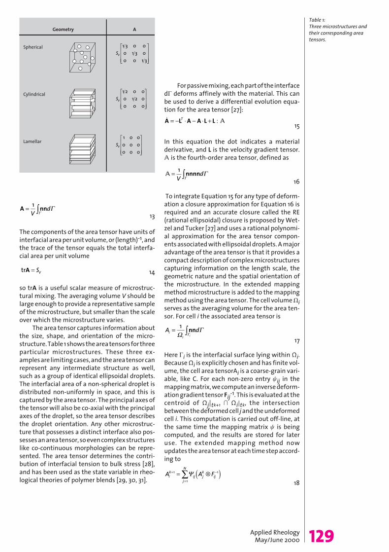
The components of the area tensor have units ofinterfacial area per unit volume, or (length)-1, andthe trace of the tensor equals the total interfa-cial area per unit volume

14

so trA is a useful scalar measure of microstruc-tural mixing. The averaging volume V should belarge enough to provide a representative sampleof the microstructure, but smaller than the scaleover which the microstructure varies.

The area tensor captures information aboutthe size, shape, and orientation of the micro-structure. Table 1 shows the area tensors for threeparticular microstructures. These three ex-amples are limiting cases, and the area tensor canrepresent any intermediate structure as well,such as a group of identical ellipsoidal droplets.The interfacial area of a non-spherical droplet isdistributed non-uniformly in space, and this iscaptured by the area tensor. The principal axes ofthe tensor will also be co-axial with the principalaxes of the droplet, so the area tensor describesthe droplet orientation. Any other microstruc-ture that possesses a distinct interface also pos-sesses an area tensor, so even complex structureslike co-continuous morphologies can be repre-sented. The area tensor determines the contri-bution of interfacial tension to bulk stress [28],and has been used as the state variable in rheo-logical theories of polymer blends [29, 30, 31].

For passive mixing, each part of the interfacedG deforms affinely with the material. This canbe used to derive a differential evolution equa-tion for the area tensor [27]:

15

In this equation the dot indicates a materialderivative, and L is the velocity gradient tensor.¿ is the fourth-order area tensor, defined as

16

To integrate Equation 15 for any type of deform-ation a closure approximation for Equation 16 isrequired and an accurate closure called the RE(rational ellipsoidal) closure is proposed by Wet-zel and Tucker [27] and uses a rational polynomi-al approximation for the area tensor compon-ents associated with ellipsoidal droplets. A majoradvantage of the area tensor is that it provides acompact description of complex microstructurescapturing information on the length scale, thegeometric nature and the spatial orientation ofthe microstructure. In the extended mappingmethod microstructure is added to the mappingmethod using the area tensor. The cell volume Wiserves as the averaging volume for the area ten-sor. For cell i the associated area tensor is

17

Here Gi is the interfacial surface lying within Ωi.Because Ωi is explicitly chosen and has finite vol-ume, the cell area tensorAi is a coarse-grain vari-able, like C. For each non-zero entry yij in themapping matrix, we compute an inverse deform-ation gradient tensor Fij-1. This is evaluated at thecentroid of Ωj|tk+1 » Ωi|tk, the intersectionbetween the deformed cell j and the undeformedcell i. This computation is carried out off-line, atthe same time the mapping matrix y is beingcomputed, and the results are stored for lateruse. The extended mapping method nowupdates the area tensor at each time step accord-ing to

18


Geometry A

Spherical

Cylindrical

Lamellar

SV

1 3 0 00 1 3 00 0 1 3

SV

1 2 0 00 1 2 00 0 0

SV

1 0 00 0 00 0 0

Table 1: Three microstructures andtheir corresponding areatensors.

Bilder 14.02.2001 10:11 Uhr Seite 129


0 0.1 0.2 0.3 0.4 0.5 0.6 0.7 0.8 0.9 1

0 0.1 0.2 0.3 0.4 0.5 0.6 0.7 0.8 0.9 1

0 0.1 0.2 0.3 0.4 0.5 0.6 0.7 0.8 0.9 1

0 0.1 0.2 0.3 0.4 0.5 0.6 0.7 0.8 0.9 1

0.5 1 1.5 2 2.5 3 3.5 4

2.5 3 3.5 4 4.5 5 5.5 6 6.5

8 8.5 9 9.5 10 10.5 11 11.5 12

2.5 3 3.5 4 4.5 5 5.5 6 6.5

Figure 10 a-f: Evolution of concentration(left) and trace of the areatensor (right) distributions

in the flow described by protocol TB-T-B with

dimensionless displacement D = 8.

Marker fluid initially fills the left half of the cavity.

The results are shown after2, 4, and 8 periods of theflow. (g, h): Similar to (c)and (d), but marker fluid

initially fills the lower halfof the cavity.

10 a 10 b

10 c 10 d

10 e 10 f

10 g 10 h

Bilder 14.02.2001 10:11 Uhr Seite 130

That is, the area tensor in any cell at time k+ 1 is the sum of contributions from all donor cells,after the donor tensors from time k have beentransformed by the appropriate deformationgradients. The symbol ƒ denotes the transform-ing of the area tensor under finite strain and isused to convert an initial area tensor A0 to anequivalent droplet shape tensor G0, find thedroplet shape tensor G in the deformed state, andthen transform G back to find the deformed-state area tensor A. Equations 9 and 18 constituteone step of the extended mapping method. Alldetails of the conversion between A and G andon the validation of the extended mappingmethod can be found in Galaktionov et al. [26]

4.1 APPLICATION TO THE 2D CAVITY FLOW:SELF-SIMILARITY OF THE MICROSTRUCTURE

For the globally chaotic flow TB-T-B with D = 8concentration distribution results are shown inFigure 10. For this protocol, the striation thick-ness of the emerging lamellar mixture patternquickly become too fine to resolve with the basicmapping technique using a 200 * 120 grid. Intrin-sic numerical errors, caused by averaging on thecell scale at every mapping step, also tend toerase the fine structure of the mixture. As aresult, after only a few periods the computedconcentration distribution is nearly uniform (Fig-ure 10e). This is a desirable mixing result on themacroscale, but in Figure 10e the pattern of cellconcentrations no longer reveals anything use-ful about the state of the mixture.

The extended mapping method compen-sates for this loss of information by tracking themicrostructure within each cell. These results areshown in Figure 10, parts b, d, e, and f. Here weshow the values of log(trA) within each cell, fordifferent times during the mixing process. Alogarithmic scale is used because the area tensordistribution is very non-uniform. Although the con-centration distribution quickly becomes nearlyuniform, the microstructure continues to evolveas mixing proceeds. In addition, the mixtureremains highly structured at the microscale, andthe interface distribution is highly non-uniform.

A self-similar pattern of interface distribu-tion is established after a few periods. This pat-tern is maintained for all subsequent mixing,while the average value of the trace of the areatensor grows exponentially. Thus, Figure 10d and

f are identical in appearance, though the two fig-ures use different scales for their gray level maps.The pattern after only two periods, Figure 10b, isonly slightly different from the self-similar pat-tern in Figure 10d and f.

For a globally chaotic flow, this self-similarpattern of the interface distribution is also inde-pendent on the initial configuration of the mix-ture. Figures 10g and h show the distributions ofconcentration and of trA after four periods of thesame flow, but for a different initial condition.Here the dark fluid initially occupies the lowerhalf of the cavity, and the initial interface is hori-zontal. Although the concentration pattern inFigure 10g is slightly different from Figure 10c, theinterface distribution in Figure 10h is identical toFigure 10d. The average value of trA in Figure 10his slightly higher than in the previous case,because the initial interface was longer. In Galak-tionov [26] the evolution of total interface isstudied in more detail.

5 CONCLUSIONSAn overview of recent work studying liquid-liquidchaotic mixing by distribution matrices is pre-sented in this paper. The computation of themapping matrix is time consuming and its com-puting can be significantly reduced by parallel-isation of the numerical code. Once the matrix iscomputed the evolution of the composition offluid concentration can be studied very fast com-pared to the computation of the mapping matrix.It is shown that the mapping method can be usedto study a large variety of 2D and 3D mixingprotocols, and that protocol parameters can beoptimised with respect to the mixing measurechosen. The results are presented for simplifiedgeometries, but the method is general and canbe applied to a wide range of mixing problems.The strength of the method is that it models mix-ing directly. One can specify the initial config-uration of the two fluids, subject them to a pre-scribed amount of mixing, and predict theconcentration distribution at every point in theresulting mixture. Moreover, it is possible toextend to algorithm not only to map concentra-tion of fluid, but also to include microstructureto the mapping: the extended mapping method.

The extended mapping method not onlyprovides explicit prediction of mixing perform-


Bilder 14.02.2001 10:11 Uhr Seite 131

ance, but also important fundamental infor-mation about the flow itself. The calculationreveals the self-replicating pattern of interfaceorientation that arises in periodic flows. Whenthe flow is globally chaotic, this pattern displaysan exponential growth rate for interfacial area.Spatial analyses of the one-period dynamics forinterface stretching can be performed, to revealwhich parts of the flow field are most effectiveat small-scale mixing.

One disadvantage of the present calculationis that it is subject to numerical diffusion. Thisrestricts its quantitative accuracy, especiallywhen studying the long-time behaviour of aflow. However, the short-time behaviour is accur-ately predicted, and we expect that the relativeperformance of different mixing protocols will bepredicted quite accurately, provided one uses thesame size mapping steps for both protocols. Thismakes the extended mapping method a usefulengineering tool.

A topic of the current research in our la-boratory, is the extension of the mappingmethod technique to more complex, industrial,mixers. Examples include the multiflux staticmixer, described by Sluijters [32], an example ofa three-dimensional space-periodic flow, and theclosely intermeshing, corotating twin screwextruder, which can be regarded as either time-or space-periodic. Moreover, an experimentalset-up of the cubic cavity flow will be used tovalidate the computational results for e.g. thefour-step mixing protocol, and to study the in-fluence of visco-elastic effects on mixing.

ACKNOWLEDGEMENTSFinancial support for this work was provided bythe Dutch Polymer Institute. Apart from theresearch staff in our group, the authors want tothank Prof. Charles Tucker of the University of Illi-nois at Urbana-Champaign for helpful discus-sions concerning the area and shape tensors.

BIOGRAPHYHan Meijer received his Ph.D. degree from theUniversity of Twente in 1980 with Prof. J.F. IngenHousz as his supervisor. He joined DSM research,and was active in the area of Polymer ProcessingModelling and Explorative Research. In 1985 hebecame part-time professor at the departmentof Polymer Chemistry and Technology in the areaof applied rheology. In 1989 he became full pro-fessor in Polymer Technology in the Division ofComputational and Experimental Mechanics ofthe Department of Mechanical Engineering. Hehas been chairman of the Dutch Society of Rhe-ology since 1995 and is currently president-electof the Polymer Processing Society. Patrick Ander-son graduated in Applied Mathematics at theUniversity of Eindhoven in 1994 under the super-vision of Prof. A.A. Reusken. He received his Ph.D.degree in the research group Materials Technol-ogy lead by Prof. H.E.H. Meijer and Prof. F.P.T.Baaijens where he studied distributive mixingprocesses. After a six month leave at Océ Tech-nologies he joined the Materials Technologygroup as an Assistant Professor.


Bilder 14.02.2001 10:11 Uhr Seite 132

REFERENCES[1] R.S. Spencer and R.H. Wiley: The mixing of very viscous

liquids, J. Colloid Sci. 6 (1951) 133-145.[2] P.G.M. Kruijt, O.S. Galaktionov, P.D. Anderson, G.W.M.

Peters, and H.E.H Meijer: Analyzing fluid mixing inperiodic flows by distribution matrices, AIChE J. (2000)submitted.

[3] H. Aref: Stirring by chaotic advection, J. Fluid Mech. 143(1984) 1-21.

[4] J.M. Ottino: The kinematics of mixing: stretching, chaosand transport, Cambridge University Press (1989).

[5] Th. Avalosse: Simulation numerique du melange lami-naire par elements finis, PhD thesis, UniversitéCatholique de Louvain, Belgium (1993).

[6] D.M. Hobbs and F.J. Muzzio: Effects of injection location,flow ratio and geometry on Kenics mixer performance,AIChE Journal 43 (1997) 3121-3132.

[7] H.A. Kusch and J.M. Ottino: Experiments on mixing incontinuous chaotic flows, J. Fluid Mech. 236 (1992) 319-348.

[8] V.V. Meleshko, O.S. Galaktionov, G.W.M. Peters, andH.E.H. Meijer: Three-dimensional mixing in Stokes flow:the partitioned pipe mixer problem revisited, Eur. J. ofMech. / Part B - Fluids 18 (1999) 783-792.

[9] V.V. Meleshko: Steady Stokes flow in a rectangular cav-ity, Proc. Roy. Soc. London A 452 (1996) 1999-2002.

[10] P.D. Anderson, O.S. Galaktionov, G.W.M. Peters, F.N. vande Vosse and H.E.H. Meijer: Analysis of mixing in three-dimensional time-periodic cavity flows, J. Fluid Mech.386 (1999) 149-166.

[11] F.J. Muzzio, P.D. Swanson, and J.M. Ottino: The statisticsof stretching and stirring in chaotic flows, Phys. Fluids 3(1991) 822-834.

[12] L.J.P. Timmermans, P.D. Minev, and F.N. van de Vosse: Anapproximate projection scheme for incompressible flowusing spectral elements, Int. J. Numer. Meth. Fluids 22(1996) 673-688.

[13] P.D. Anderson: Computational Analysis of DistributiveMixing, PhD thesis, Eindhoven University of Technology,The Netherlands (1999).

[14] Y.Maday and A.T. Patera: Spectral element methods forthe incompressible Navier-Stokes equations, In A.Noor,editor, State-of-the-Art surveys on computationalmechanics, ASME, New York (1989).

[15] O.S. Galaktionov, P.D. Anderson, and G.W.M. Peters:Symmetry of periodic structures in a 3D mixing cavityflow, Phys. Fluids 12 (2000) 469-471.

[16] O.S. Galaktionov, P.D. Anderson, G.W.M. Peters, and F.N.van de Vosse: An adaptive front tracking technique forthree-dimensional transient flows, Int. J. Numer. Meth.Fluids 32 (2000) 201-217.

[17] P.V. Danckwerts: The definition and measurement ofsome characteristics of mixtures, Appl. Sci. Res. A 3 (1953)279-296.

[18] J.G. Franjione, C.Leong, and J.M. Ottino: Symmetrieswithin chaos: A route to effective mixing, Phys. of FluidsA 1 (1989) 1772-1783.

[19] S.C. Jana, G.Metcalfe, and J.M. Ottino: Experimental andcomputational studies of mixing in complex Stokesflows: The vortex mixing flow and multicellular cavityflows, J. Fluid Mech. 269 (1994) 199-246.

[20] H.Aref and M.S. Naschie: Chaos Applied to Fluid Mixing,Elsevier Science Ltd., London (1995).

[21] P.D. Anderson, O.S. Galaktionov, G.W.M. Peters, F.N. vande Vosse, and H.E.H. Meijer: Mixing of non-Newtonianfluids in time-periodic cavity flows, J. Non-Newt. FluidMech. (2000) Accepted.

[22] O.S. Galaktionov, P.D. Anderson, P.G.M. Kruijt, G.W.M.Peters, and H.E.H. Meijer: A mapping approach for 3Ddistributive mixing analysis, Computers & Fluids (2000)Accepted.

[23] R.Chella and J.Viñals: Mixing of a two-phase fluid by cav-ity flow, Phys. Rev. E 53 (1996) 3832-3840.

[24] F.J. Muzzio, C.Meneveau, P.D. Swanson, and J.M. Ottino:Scaling and multifractal properties of mixing in chaot-ic flows, Phys. Fluids 4 (1991) 1439-1456.

[25] M.Liu, R.L. Peshkin, F.J. Muzzio, and C.W. Leong: Struc-ture of the stretching field in chaotic cavity flows, AIChEJ. 40 (1994) 1273-1286.

[26] O.S. Galaktionov, P.D. Anderson, G.W.M. Peters, andCharles L.Tucker III: A global, multi-scale simulation oflaminar fluid mixing: The extended mapping method,Int. J. of Multiphase Flows (2000) Submitted.

[27] E.D. Wetzel and C.L. Tucker: Area tensors for modelingmicrostructure during laminar liquid-liquid mixing, Int.J. Multiphase Flow 25 (1999) 35-61.

[28] C.E. Rosenkilde: Surface-energy tensors, J. Math. Phys. 8(1967) 84-97.

[29] M. Doi and T. Ohta: Dynamics and rheology of complexinterfaces I, J. Chem. Phys. 95 (1991) 1242-1248.

[30] M. Grmela and A.Ait-Kadi: Rheology of inhomogeneousimmiscible blends, J. Non-Newt. Fluid Mech. 77 (1998)191-199.

[31] N.J. Wagner, H.C. Õttinger and B.J. Edwards: GeneralizedDoi-Ohta model for multiphase flow developed viaGENERIC, AIChE J. 45 (1999) 1169-1181.

[32] R.Sluijters: Het principe van de multiflux menger, Inge-nieur of Chemische Techniek 77 (1965) 33-36 (in Dutch)


Bilder 14.02.2001 10:11 Uhr Seite 133

chaotic mixing analyses by distribution matrices

Documents