chap 3 : two random variables - ryerson universitycourses/ee8103/chap3.pdf · chap 3: two random...
TRANSCRIPT
Chap 3: Two Random Variables
Chap 3 : Two Random Variables
Chap 3.1: Distribution Functions of Two RVs
In many experiments, the observations are expressible not as a single quantity, but as a familyof quantities. For example to record the height and weight of each person in a community orthe number of people and the total income in a family, we need two numbers.
Let X and Y denote two random variables based on a probability model (Ω, F, P ). Then
P (x1 < X(ξ) ≤ x2) = FX(x2) − FX(x1) =∫ x2
x1
fX(x) dx
and
P (y1 < Y (ξ) ≤ y2) = FY (y2) − FY (y1) =∫ y2
y1
fY (y) dy
What about the probability that the pair of RVs (X,Y ) belongs to an arbitrary region D? Inother words, how does one estimate, for example
P [(x1 < X(ξ) ≤ x2) ∩ (y1 < Y (ξ) ≤ y2)] =?
Towards this, we define the joint probability distribution function of X and Y to be
FXY (x, y) = P (X ≤ x, Y ≤ y) ≥ 0 (1)
1
.

Chap 3: Two Random Variables
where x and y are arbitrary real numbers.
Properties
1.
FXY (−∞, y) = FXY (x,−∞) = 0, FXY (+∞, +∞) = 1 (2)
since (X(ξ) ≤ −∞, Y (ξ) ≤ y) ⊂ (X(ξ) ≤ −∞), we get
FXY (−∞, y) ≤ P (X(ξ) ≤ −∞) = 0
Similarly, (X(ξ) ≤ +∞, Y (ξ) ≤ +∞) = Ω, we get FXY (+∞, +∞) = P (Ω) = 1.
2.
P (x1 < X(ξ) ≤ x2, Y (ξ) ≤ y) = FXY (x2, y) − FXY (x1, y) (3)
P (X(ξ) ≤ x, y1 < Y (ξ) ≤ y2) = FXY (x, y2) − FXY (x, y1) (4)
To prove (3), we note that for x2 > x1
(X(ξ) ≤ x2, Y (ξ) ≤ y) = (X(ξ) ≤ x1, Y (ξ) ≤ y) ∪ (x1 < X(ξ) ≤ x2, Y (ξ) ≤ y)
2
Chap 3: Two Random Variables
and the mutually exclusive property of the events on the right side gives
P (X(ξ) ≤ x2, Y (ξ) ≤ y) = P (X(ξ) ≤ x1, Y (ξ) ≤ y)+P (x1 < X(ξ) ≤ x2, Y (ξ) ≤ y)
which proves (3). Similarly (4) follows.
3.
P (x1 < X(ξ) ≤ x2, y1 < Y (ξ) ≤ y2) = FXY (x2, y2) − FXY (x2, y1) (5)
−FXY (x1, y2) + FXY (x1, y1)
This is the probability that (X, Y ) belongs to the rectangle in Fig. 3. To prove (5), wecan make use of the following identity involving mutually exclusive events on the rightside.
(x1 < X(ξ) ≤ x2, Y (ξ) ≤ y2) = (x1 < X(ξ) ≤ x2, Y (ξ) ≤ y1)
∪(x1 < X(ξ) ≤ x2, y1 < Y (ξ) ≤ y2)
This gives
P (x1 < X(ξ) ≤ x2, Y (ξ) ≤ y2) = P (x1 < X(ξ) ≤ x2, Y (ξ) ≤ y1)
+P (x1 < X(ξ) ≤ x2, y1 < Y (ξ) ≤ y2)
3

Chap 3: Two Random Variables
and the desired result in (5) follows by making use of (3) with y = y2 and y1
respectively.
Figure 1: Two dimensional RV.
4
Chap 3: Two Random Variables
Joint Probability Density Function (Joint pdf)
By definition, the joint pdf of X and Y is given by
fXY (x, y) =∂2FXY (x, y)
∂x∂y(6)
and hence we obtain the useful formula
FXY (x, y) =∫ x
−∞
∫ y
−∞fXY (u, v) du dv (7)
Using (2), we also get ∫ ∞
−∞
∫ ∞
−∞fXY (x, y) = 1 (8)
P ((X, Y ) ∈ D) =∫ ∫
(x,y)∈D
fXY (x, y) dx dy (9)
5
dxdy = 1
Chap 3: Two Random Variables
Marginal Statistics
In the context of several RVs, the statistics of each individual ones are called marginalstatistics. Thus FX(x) is the marginal probability distribution function of X , and fX(x) isthe marginal pdf of X . It is interesting to note that all marginal can be obtained from the jointpdf. In fact
FX(x) = FXY (x,+∞) FY (y) = FXY (+∞, y) (10)
Also
fX(x) =∫ ∞
−∞fXY (x, y)dy fY (y) =
∫ ∞
−∞fXY (x, y)dx. (11)
To prove (10), we can make use of the identity
(X ≤ x) = (X ≤ x) ∩ (Y ≤ +∞)
so that
FX(x) = P (X ≤ x) = P (X ≤ x, Y ≤ ∞) = FXY (x,+∞) (12)
6
Chap 3: Two Random Variables
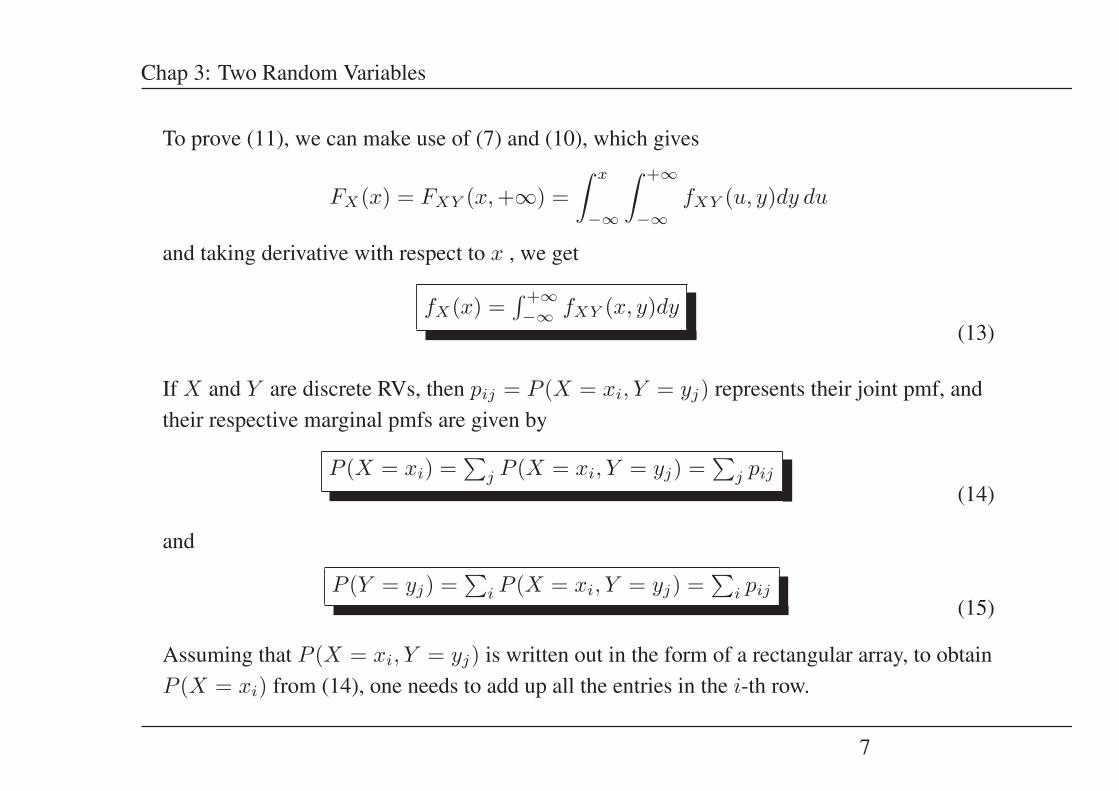
To prove (11), we can make use of (7) and (10), which gives
FX(x) = FXY (x,+∞) =∫ x
−∞
∫ +∞
−∞fXY (u, y)dy du
and taking derivative with respect to x , we get
fX(x) =∫ +∞−∞ fXY (x, y)dy
(13)
If X and Y are discrete RVs, then pij = P (X = xi, Y = yj) represents their joint pmf, andtheir respective marginal pmfs are given by
P (X = xi) =∑
j P (X = xi, Y = yj) =∑
j pij
(14)
and
P (Y = yj) =∑
i P (X = xi, Y = yj) =∑
i pij
(15)
Assuming that P (X = xi, Y = yj) is written out in the form of a rectangular array, to obtainP (X = xi) from (14), one needs to add up all the entries in the i-th row.
7

Chap 3: Two Random Variables
Figure 2: Illustration of marginal pmf.
It used to be a practice for insurance companies routinely to scribble out these sum values inthe left and top margins, thus suggesting the name marginal densities! (Fig 2).
8

Chap 3: Two Random Variables
Examples
From (11) and (12), the joint CDF and/or the joint pdf represent complete information aboutthe RVs, and their marginal pdfs can be evaluated from the joint pdf. However, givenmarginals, (most often) it will not be possible to compute the joint pdf.
Example 1: Given
fXY (x, y) =
⎧⎨⎩ constant 0 < x < y < 1
0 o.w.(16)
Obtain the marginal pdfs fX(x) and fY (y).
Solution: It is given that the joint pdf fXY (x, y) is a constant in the shaded region in Fig. 3.We can use (8) to determine that constant c. From (8)∫ +∞
−∞
∫ +∞
−∞fXY (x, y)dx dy =
∫ 1
y=0
(∫ y
x=0
c · dx
)dy =
∫ 1
y=0
cy dy =cy2
2
∣∣∣10 =c
2= 1
9
c

Chap 3: Two Random Variables
Figure 3: Diagram for the example.
Thus c = 2. Moreover
fX(x) =∫ +∞
−∞fXY (x, y)dy =
∫ 1
y=x
2dy = 2(1 − x) 0 < x < 1
and similarly,
fY (y) =∫ +∞
−∞fXY (x, y)dx =
∫ y
x=0
2 dx = 2y 0 < y < 1
10
Chap 3: Two Random Variables
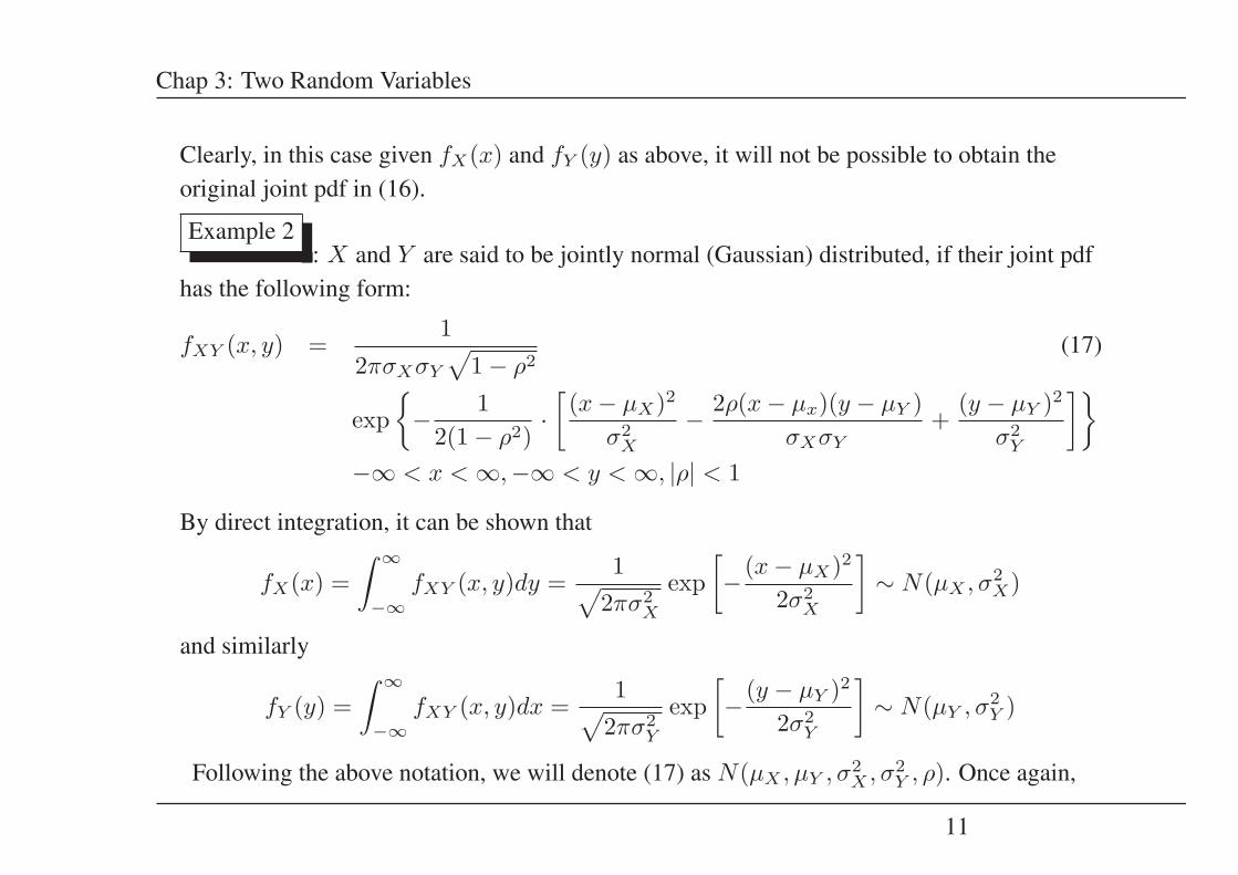
Clearly, in this case given fX(x) and fY (y) as above, it will not be possible to obtain theoriginal joint pdf in (16).
Example 2: X and Y are said to be jointly normal (Gaussian) distributed, if their joint pdf
has the following form:
fXY (x, y) =1
2πσXσY
√1 − ρ2
(17)
exp{− 1
2(1 − ρ2)·[(x − μX)2
σ2X
− 2ρ(x − μx)(y − μY )σXσY
+(y − μY )2
σ2Y
]}−∞ < x < ∞,−∞ < y < ∞, |ρ| < 1
By direct integration, it can be shown that
fX(x) =∫ ∞
−∞fXY (x, y)dy =
1√2πσ2
X
exp[− (x − μX)2
2σ2X
]∼ N(μX , σ2
X)
and similarly
fY (y) =∫ ∞
−∞fXY (x, y)dx =
1√2πσ2
Y
exp[− (y − μY )2
2σ2Y
]∼ N(μY , σ2
Y )
Following the above notation, we will denote (17) as N(μX , μY , σ2X , σ2
Y , ρ). Once again,
11
Chap 3: Two Random Variables
knowing the marginals in above alone doesn’t tell us everything about the joint pdf in (17).As we show below, the only situation where the marginal pdfs can be used to recover thejoint pdf is when the random variables are statistically independent.
12
Chap 3: Two Random Variables
Independence of RVs
Definition: The random variables X and Y are said to be statistically independent if
P [(X(ξ) ≤ x) ∩ (Y (ξ) ≤ y)] = P (X(ξ) ≤ x) · P (Y (ξ) ≤ y)
• For continuous RVs,
FXY (x, y) = FX(x) · FY (y) (18)
or equivalently, if X and Y are independent, then we must have
fXY (x, y) = fX(x) · fY (y) (19)
• If X and Y are discrete-type RVs then their independence implies
P (X = xi, Y = yj) = P (X = xi) · P (Y = yj) for all i, j (20)
Equations (18)-(20) give us the procedure to test for independence. Given fXY (x, y), obtainthe marginal pdfs fX(x) and fY (y) and examine whether one of the equations in (18) or (20)is valid. If so, the RVs are independent, otherwise they are dependent.
• Returning back to Example 1, we observe by direct verification that
13
Chap 3: Two Random Variables
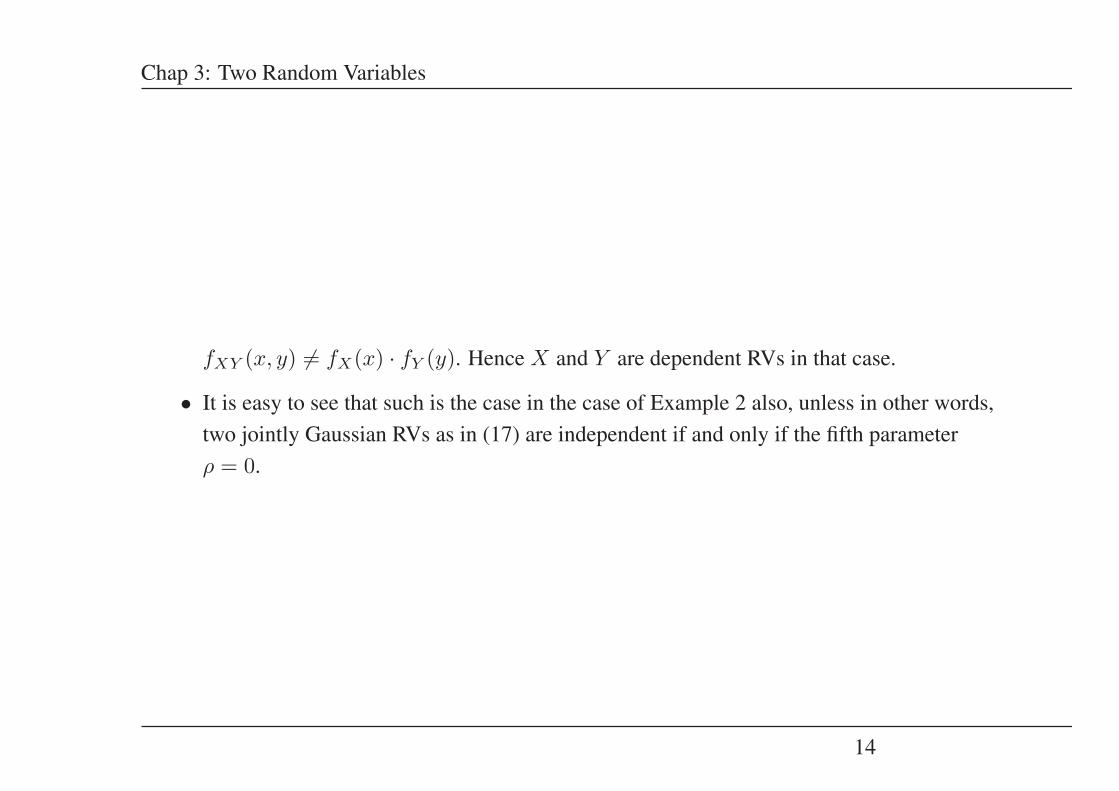
fXY (x, y) = fX(x) · fY (y). Hence X and Y are dependent RVs in that case.
• It is easy to see that such is the case in the case of Example 2 also, unless in other words,two jointly Gaussian RVs as in (17) are independent if and only if the fifth parameterρ = 0.
14

Chap 3: Two Random Variables
Expectation of Functions of RVs
If X and Y are random variables and g(·) is a function of two variables, then
E[g(X, Y )] =∑
y
∑x
g(x, y) p(x, y) discrete case
=∫ ∞
−∞
∫ ∞
−∞g(x, y)f(x, y) dx dy continuous case
If g(X, Y ) = aX + bY , then we can obtain
E[aX + bY ] = aE[X] + bE[Y ]
Example 3At a party N men throw their hats into the center of a room. The hats are
mixed up and each man randomly selects one. Find the expected number of men who selecttheir own hats.
Solution: let X denote the number of men that select their own hats, we can compute E[X]by noting that
X = X1 + X2 + · · · + XN
15
Chap 3: Two Random Variables
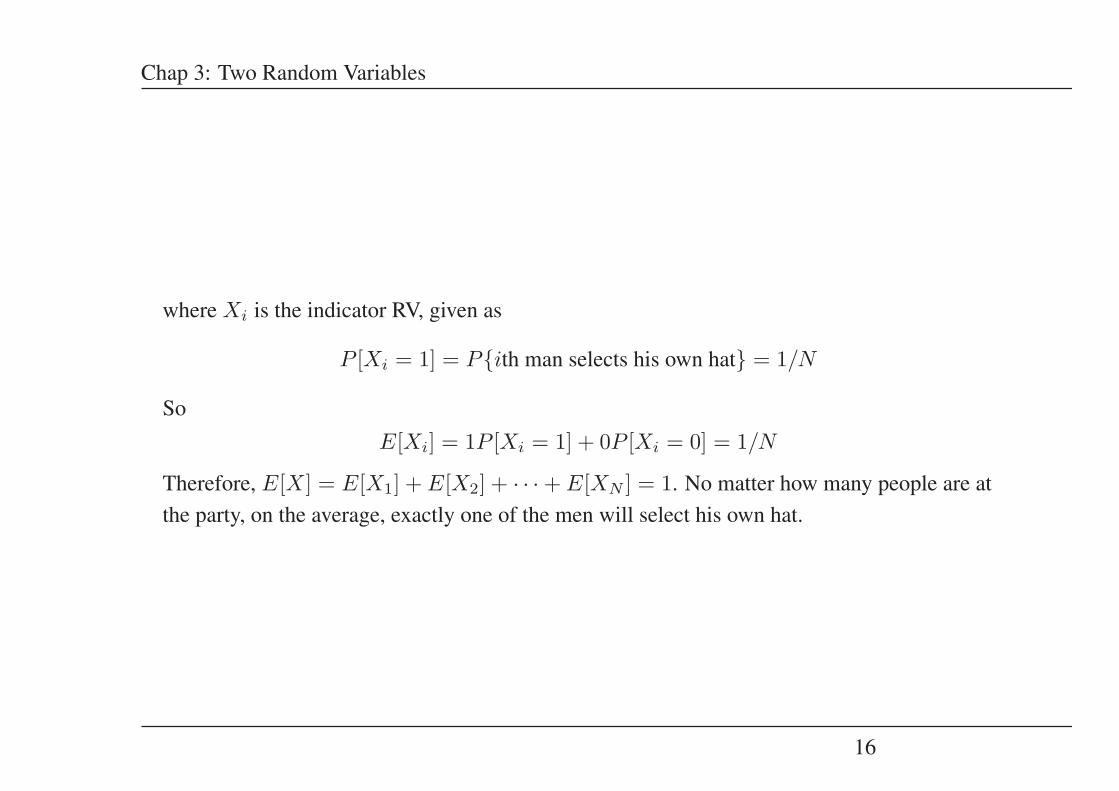
where Xi is the indicator RV, given as
P [Xi = 1] = P{ith man selects his own hat} = 1/N
SoE[Xi] = 1P [Xi = 1] + 0P [Xi = 0] = 1/N
Therefore, E[X] = E[X1] + E[X2] + · · · + E[XN ] = 1. No matter how many people are atthe party, on the average, exactly one of the men will select his own hat.
16
Chap 3: Two Random Variables
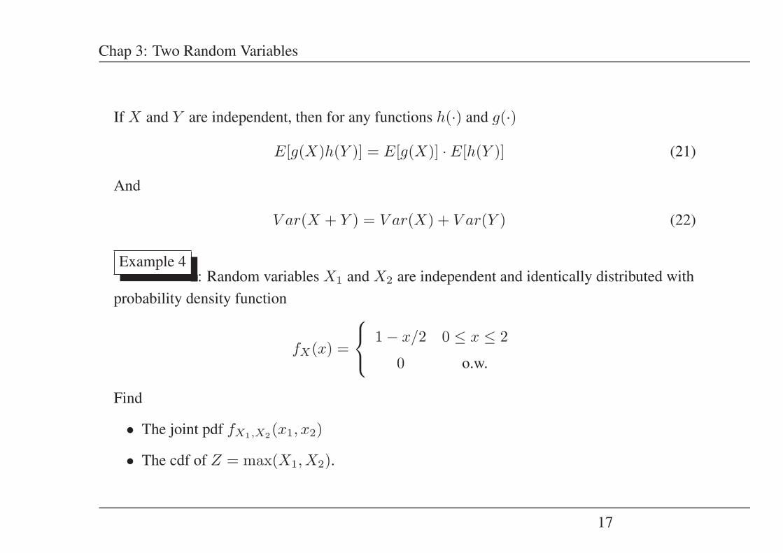
If X and Y are independent, then for any functions h(·) and g(·)
E[g(X)h(Y )] = E[g(X)] · E[h(Y )] (21)
And
V ar(X + Y ) = V ar(X) + V ar(Y ) (22)
Example 4: Random variables X1 and X2 are independent and identically distributed with
probability density function
fX(x) =
⎧⎨⎩ 1 − x/2 0 ≤ x ≤ 2
0 o.w.
Find
• The joint pdf fX1,X2(x1, x2)
• The cdf of Z = max(X1, X2).
17
Chap 3: Two Random Variables
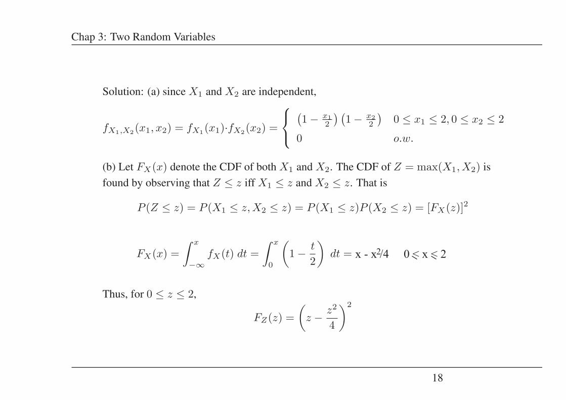
Solution: (a) since X1 and X2 are independent,
fX1,X2(x1, x2) = fX1(x1)·fX2(x2) =
⎧⎨⎩
(1 − x1
2
) (1 − x2
2
)0 ≤ x1 ≤ 2, 0 ≤ x2 ≤ 2
0 o.w.
(b) Let FX(x) denote the CDF of both X1 and X2. The CDF of Z = max(X1, X2) isfound by observing that Z ≤ z iff X1 ≤ z and X2 ≤ z. That is
P (Z ≤ z) = P (X1 ≤ z, X2 ≤ z) = P (X1 ≤ z)P (X2 ≤ z) = [FX(z)]2
FX(x) =∫ x
−∞fX(t) dt =
∫ x
0
(1 − t
2
)dt =
⎧⎪⎪⎨⎪⎪⎩
0 x < 0
x − x2
4 0 ≤ x ≤ 2
1 x > 2
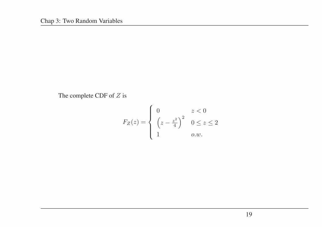
Thus, for 0 ≤ z ≤ 2,
FZ(z) =(
z − z2
4
)2
18
x - x /4 0 < x < 22
Chap 3: Two Random Variables
The complete CDF of Z is
FZ(z) =
⎧⎪⎪⎪⎨⎪⎪⎪⎩
0 z < 0(z − z2
4
)2
0 ≤ z ≤ 2
1 o.w.
19

Chap 3: Two Random Variables
Example 5: Given
fXY (x, y) =
⎧⎨⎩ xy2e−y 0 < y < ∞, 0 < x < 1
0 o.w.
Determine whether X and Y are independent.
Solution:
fX(x) =∫ +∞
0
fXY (x, y)dy = x
∫ +∞
0
y2e−ydy = x
∫ +∞
0
−y2 de−y
= x
(−y2e−y
∣∣∣∣∞0 + 2∫ +∞
0
ye−ydy
)= 2x, 0 < x < 1
Similarly
fY (y) =∫ 1
0
fXY (x, y)dx =y2
2e−y, 0 < y < ∞
In this casefXY (x, y) = fX(x) · fY (y)
and hence X and Y are independent random variables.
20
Chap 3: Two Random Variables
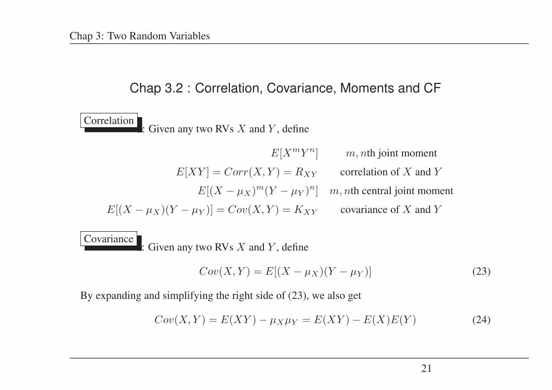
Chap 3.2 : Correlation, Covariance, Moments and CF
Correlation: Given any two RVs X and Y , define
E[XmY n] m,nth joint moment
E[XY ] = Corr(X, Y ) = RXY correlation of X and Y
E[(X − μX)m(Y − μY )n] m,nth central joint moment
E[(X − μX)(Y − μY )] = Cov(X, Y ) = KXY covariance of X and Y
Covariance: Given any two RVs X and Y , define
Cov(X, Y ) = E[(X − μX)(Y − μY )] (23)
By expanding and simplifying the right side of (23), we also get
Cov(X, Y ) = E(XY ) − μXμY = E(XY ) − E(X)E(Y ) (24)
21

Chap 3: Two Random Variables
Correlation coefficientbetween X and Y .
ρXY =Cov(X, Y )√
V ar(X)V ar(Y )=
Cov(X,Y )σXσY
− 1 ≤ ρXY ≤ 1 (25)
Cov(X,Y ) = ρXY σXσY (26)
Uncorrelated RVs: If ρXY = 0, then X and Y are said to be uncorrelated RVs. If X and Y
are uncorrelated, thenE(XY ) = E(X)E(Y ) (27)
Orthogonality: X and Y are said to be orthogonal if
E(XY ) = 0 (28)
From above, if either X or Y has zero mean, then orthogonality implies uncorrelatedness andvice-versa.
Suppose X and Y are independent RVs,
E(XY ) = E(X)E(Y ) (29)
22
Chap 3: Two Random Variables
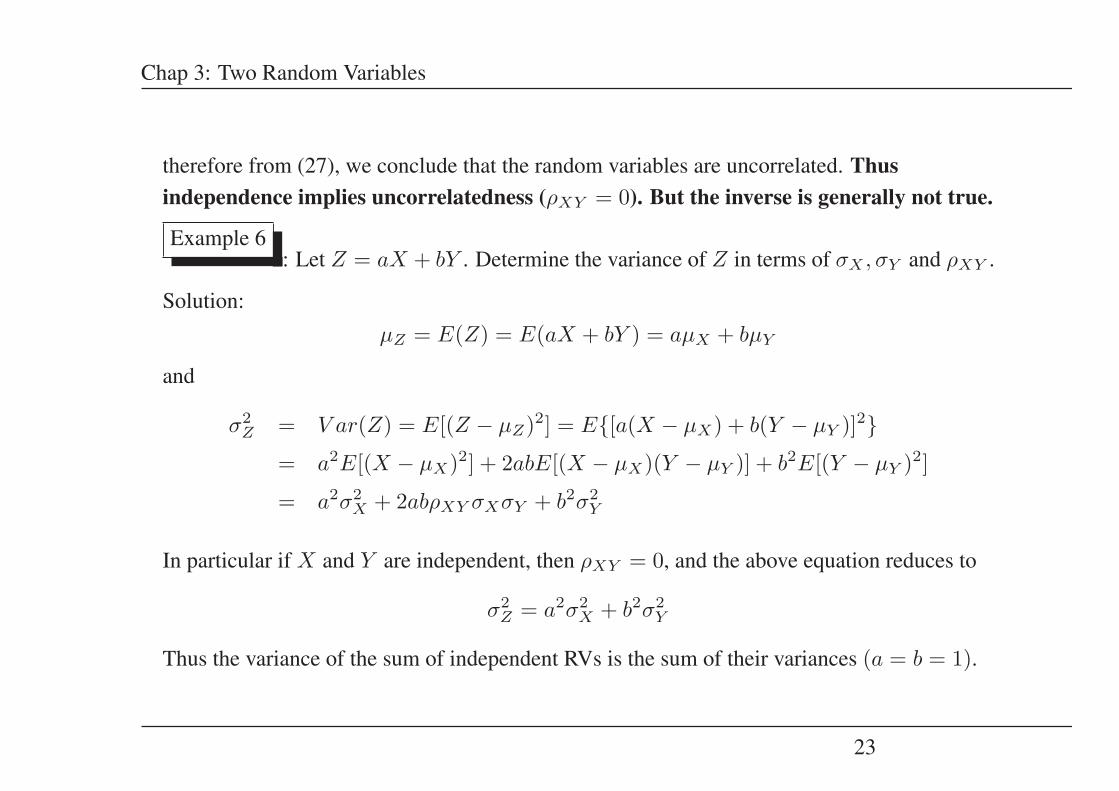
therefore from (27), we conclude that the random variables are uncorrelated. Thusindependence implies uncorrelatedness (ρXY = 0). But the inverse is generally not true.
Example 6: Let Z = aX + bY . Determine the variance of Z in terms of σX , σY and ρXY .
Solution:μZ = E(Z) = E(aX + bY ) = aμX + bμY
and
σ2Z = V ar(Z) = E[(Z − μZ)2] = E{[a(X − μX) + b(Y − μY )]2}
= a2E[(X − μX)2] + 2abE[(X − μX)(Y − μY )] + b2E[(Y − μY )2]
= a2σ2X + 2abρXY σXσY + b2σ2
Y
In particular if X and Y are independent, then ρXY = 0, and the above equation reduces to
σ2Z = a2σ2
X + b2σ2Y
Thus the variance of the sum of independent RVs is the sum of their variances (a = b = 1).
23
Chap 3: Two Random Variables
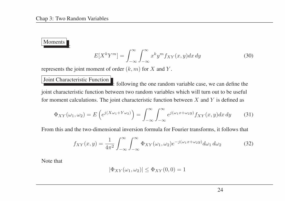
Moments:
E[XkY m] =∫ ∞
−∞
∫ ∞
−∞xkymfXY (x, y)dx dy (30)
represents the joint moment of order (k, m) for X and Y .
Joint Characteristic Function: following the one random variable case, we can define the
joint characteristic function between two random variables which will turn out to be usefulfor moment calculations. The joint characteristic function between X and Y is defined as
ΦXY (ω1, ω2) = E(ej(Xω1+Y ω2)
)=∫ ∞
−∞
∫ ∞
−∞ej(ω1x+ω2y)fXY (x, y)dx dy (31)
From this and the two-dimensional inversion formula for Fourier transforms, it follows that
fXY (x, y) =1
4π2
∫ ∞
−∞
∫ ∞
−∞ΦXY (ω1, ω2)e−j(ω1x+ω2y)dω1 dω2 (32)
Note that|ΦXY (ω1, ω2)| ≤ ΦXY (0, 0) = 1
24
Chap 3: Two Random Variables
If X and Y are independent RVs, then from (31), we obtain
ΦXY (ω1, ω2) = E(ej(ω1X)
)E(ej(ω2Y )
)= ΦX(ω1) ΦY (ω2) (33)
AlsoΦX(ω) = ΦXY (ω, 0) ΦY (ω) = ΦXY (0, ω) (34)
IndependenceIf the RV X and Y are independent, then
E[ej(ω1X+ω2Y )
]= E[ejω1X ] · E[ejω2Y ]
From this it follows thatΦ(ω1, ω2) = ΦX(ω1) · ΦY (ω2)
conversely, if above equation is true, then the random variables X and Y are independent.
ConvolutionCharacteristic functions are useful in determining the pdf of linear
combinations of RVs. If the RV X and Y are independent and Z = X + Y , then
E[ejωZ
]= E
[ejω(X+Y )
]= E
[ejωX
] · E [ejωY
]
25
Product
Chap 3: Two Random Variables
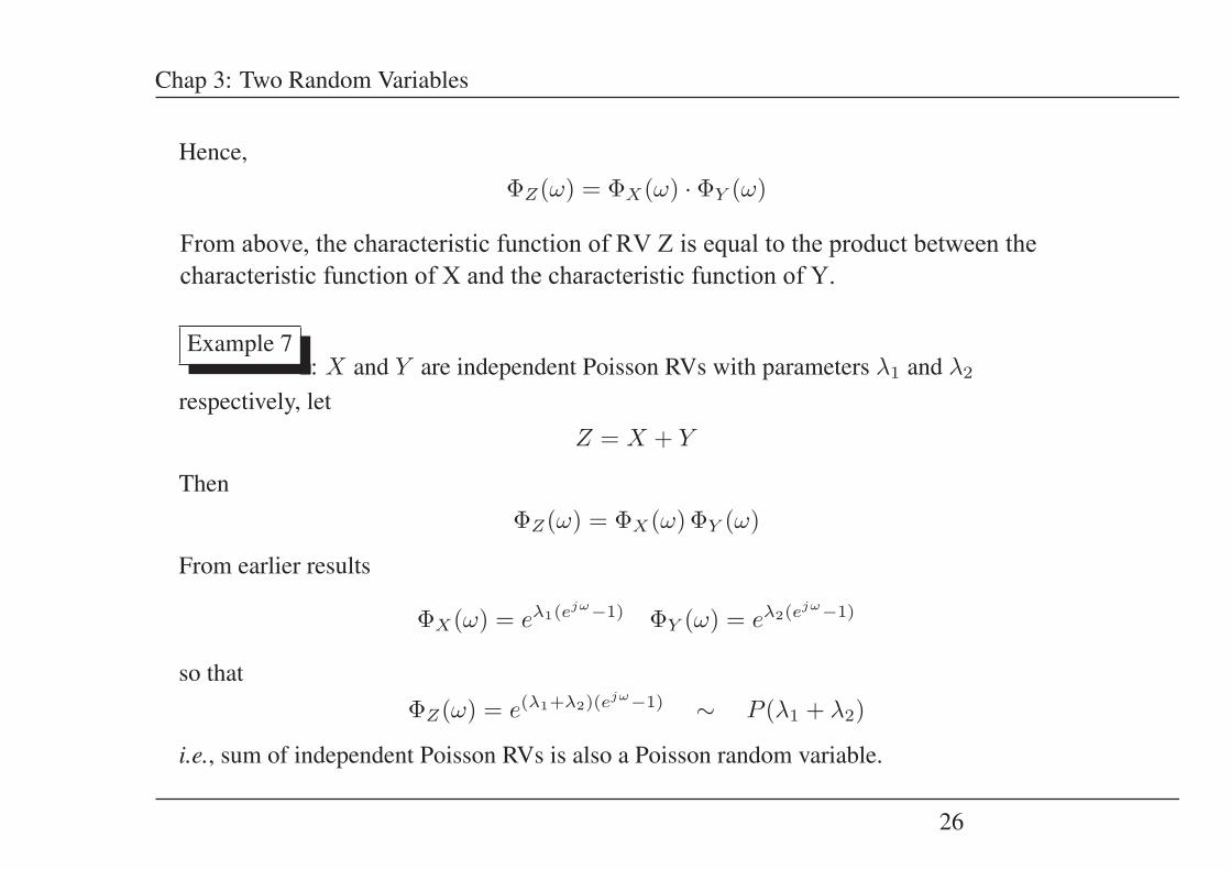
Hence,ΦZ(ω) = ΦX(ω) · ΦY (ω)
It is known that the density of Z equals the convolution of fX(x) and fY (y). From above,the characteristic function of the convolution of two densities equals the product of theircharacteristic functions.
Example 7: X and Y are independent Poisson RVs with parameters λ1 and λ2
respectively, letZ = X + Y
ThenΦZ(ω) = ΦX(ω) ΦY (ω)
From earlier results
ΦX(ω) = eλ1(ejω−1) ΦY (ω) = eλ2(e
jω−1)
so thatΦZ(ω) = e(λ1+λ2)(e
jω−1) ∼ P (λ1 + λ2)
i.e., sum of independent Poisson RVs is also a Poisson random variable.
26
From above, the characteristic function of RV Z is equal to the product between the characteristic function of X and the characteristic function of Y.
Chap 3: Two Random Variables
Chap 3.3 : Gaussian RVs and Central Limit Theorem
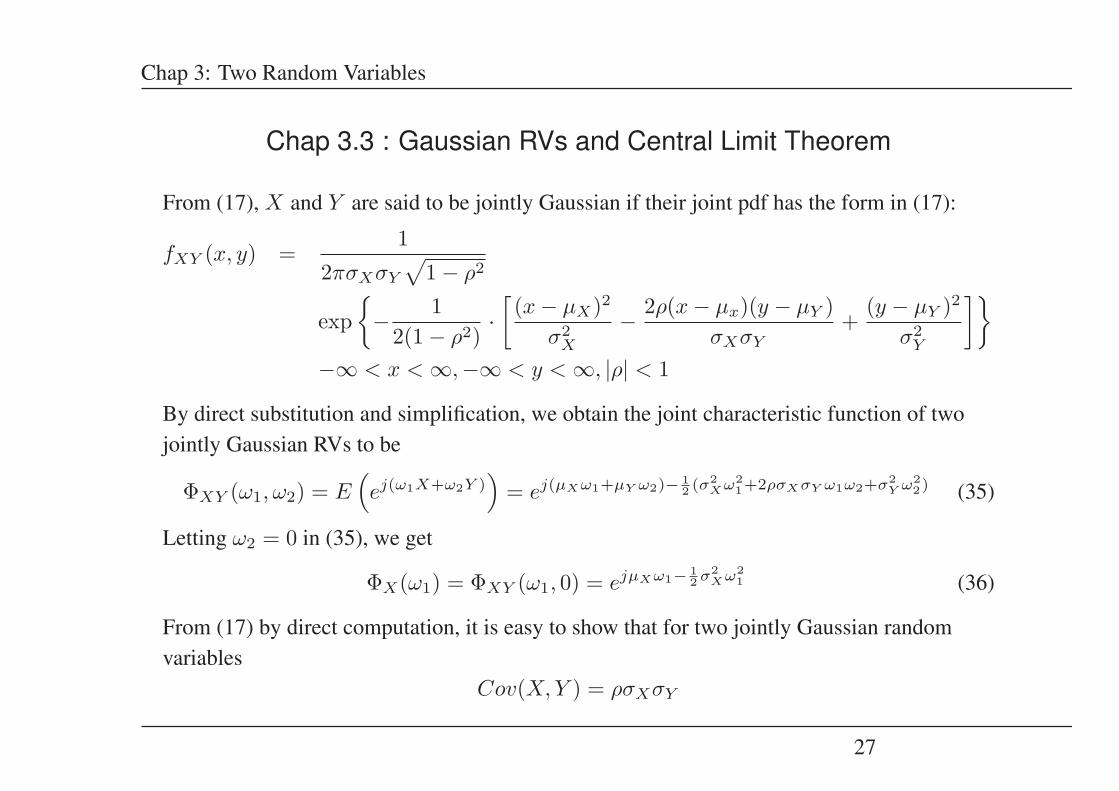
From (17), X and Y are said to be jointly Gaussian if their joint pdf has the form in (17):
fXY (x, y) =1
2πσXσY
√1 − ρ2
exp{− 1
2(1 − ρ2)·[(x − μX)2
σ2X
− 2ρ(x − μx)(y − μY )σXσY
+(y − μY )2
σ2Y
]}−∞ < x < ∞,−∞ < y < ∞, |ρ| < 1
By direct substitution and simplification, we obtain the joint characteristic function of twojointly Gaussian RVs to be
ΦXY (ω1, ω2) = E(ej(ω1X+ω2Y )
)= ej(μXω1+μY ω2)− 1
2 (σ2Xω2
1+2ρσXσY ω1ω2+σ2Y ω2
2) (35)
Letting ω2 = 0 in (35), we get
ΦX(ω1) = ΦXY (ω1, 0) = ejμXω1− 12 σ2
Xω21 (36)
From (17) by direct computation, it is easy to show that for two jointly Gaussian randomvariables
Cov(X, Y ) = ρσXσY
27
Chap 3: Two Random Variables
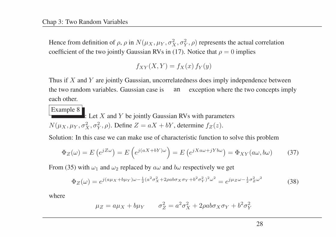
Hence from definition of ρ, ρ in N(μX , μY , σ2X , σ2
Y , ρ) represents the actual correlationcoefficient of the two jointly Gaussian RVs in (17). Notice that ρ = 0 implies
fXY (X,Y ) = fX(x) fY (y)
Thus if X and Y are jointly Gaussian, uncorrelatedness does imply independence betweenthe two random variables. Gaussian case is the only exception where the two concepts implyeach other.
Example 8: Let X and Y be jointly Gaussian RVs with parameters
N(μX , μY , σ2X , σ2
Y , ρ). Define Z = aX + bY , determine fZ(z).
Solution: In this case we can make use of characteristic function to solve this problem
ΦZ(ω) = E(ejZω
)= E
(ej(aX+bY )ω
)= E
(ejXaω+jY bω
)= ΦXY (aω, bω) (37)
From (35) with ω1 and ω2 replaced by aω and bω respectively we get
ΦZ(ω) = ej(aμX+bμY )ω− 12 (a2σ2
X+2ρabσXσY +b2σ2Y )2ω2
= ejμZω− 12 σ2
Zω2(38)
whereμZ = aμX + bμY σ2
Z = a2σ2X + 2ρabσXσY + b2σ2
Y
28
an
Chap 3: Two Random Variables
Notice that (38) has the same form as (36), and hence we conclude that Z = aX + bY is alsoGaussian with mean and variance as above, which also agrees with previous example.
From the previous example, we conclude that any linear combination of jointly Gaussian RVsgenerates a new Gaussian RV. In other words, linearity preserves Gaussianity.
Gaussian random variables are also interesting because of the following result.
29
Chap 3: Two Random Variables
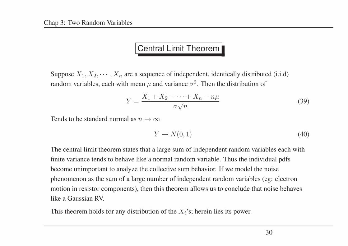
Central Limit Theorem
Suppose X1, X2, · · · , Xn are a sequence of independent, identically distributed (i.i.d)random variables, each with mean μ and variance σ2. Then the distribution of
Y =X1 + X2 + · · · + Xn − nμ
σ√
n(39)
Tends to be standard normal as n → ∞
Y → N(0, 1) (40)
The central limit theorem states that a large sum of independent random variables each withfinite variance tends to behave like a normal random variable. Thus the individual pdfsbecome unimportant to analyze the collective sum behavior. If we model the noisephenomenon as the sum of a large number of independent random variables (eg: electronmotion in resistor components), then this theorem allows us to conclude that noise behaveslike a Gaussian RV.
This theorem holds for any distribution of the Xi’s; herein lies its power.
30
Chap 3: Two Random Variables
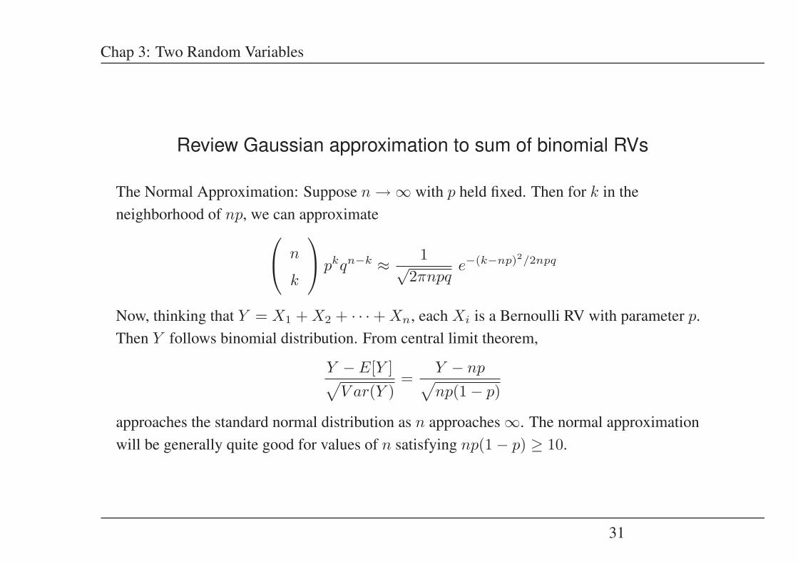
Review Gaussian approximation to sum of binomial RVs
The Normal Approximation: Suppose n → ∞ with p held fixed. Then for k in theneighborhood of np, we can approximate⎛
⎝ n
k
⎞⎠ pkqn−k ≈ 1√
2πnpqe−(k−np)2/2npq
Now, thinking that Y = X1 + X2 + · · · + Xn, each Xi is a Bernoulli RV with parameter p.Then Y follows binomial distribution. From central limit theorem,
Y − E[Y ]√V ar(Y )
=Y − np√np(1 − p)
approaches the standard normal distribution as n approaches ∞. The normal approximationwill be generally quite good for values of n satisfying np(1 − p) ≥ 10.
31

Chap 3: Two Random Variables
Example 9: The lifetime of a special type of battery is a random variable with mean 40
hours and standard deviation 20 hours. A battery is used until it fails, at which point it isreplaced by a new one. Assuming a stockpile of 25 such batteries, the lifetimes of which areindependent, approximate the probability that over 1100 hours of use can be obtained.
Solution: if we let Xi denote the lifetime of the ith battery to be put in use, andY = X1 + X2 + · · · + X25. Then we want to find P (Y > 1100).
32

Chap 3: Two Random Variables
Chap 3.4 : Conditional Probability Density Functions
For any two events A and B, we have defined the conditional probability of A given B as
P (A|B) =P (A ∩ B)
P (B), P (B) = 0 (41)
Noting that the probability distribution function FX(x) is given by FX(x) = P{X(ξ) ≤ x},we may define the conditional distribution of the RV X given the event B as
FX(x|B) = P{X(ξ) ≤ x|B} =P{(X(ξ) ≤ x) ∩ B}
P (B)(42)
In general, event B describes some property of X . Thus the definition of the conditionaldistribution depends on conditional probability, and since it obeys all probability axioms, itfollows that the conditional distribution has the same properties as any distribution function.In particular
FX(+∞|B) =P{(X(ξ) ≤ +∞) ∩ B}
P (B)=
P (B)P (B)
= 1 (43)
FX(−∞|B) =P{(X(ξ) ≤ −∞) ∩ B}
P (B)=
P (φ)P (B)
= 0
33

Chap 3: Two Random Variables
Furthermore, since for x2 ≥ x1
(X(ξ) ≤ x2) = (X(ξ) ≤ x1) ∪ (x1 < X(ξ) ≤ x2)
P (x1 < X(ξ) ≤ x2|B) =P{(x1 < X(ξ) ≤ x2) ∩ B}
P (B)= FX(x2|B) − FX(x1|B). (44)
The conditional density function is the derivative of the conditional distribution function.Thus
fX(x|B) =d
dxFX(x|B)
we obtain
FX(x|B) =∫ x
−∞ fX(u|B) du(45)
Using above equation, we can also have
P (x1 < X(ξ) ≤ x2|B) =∫ x2
x1fX(x|B) dx
(46)
34

Chap 3: Two Random Variables
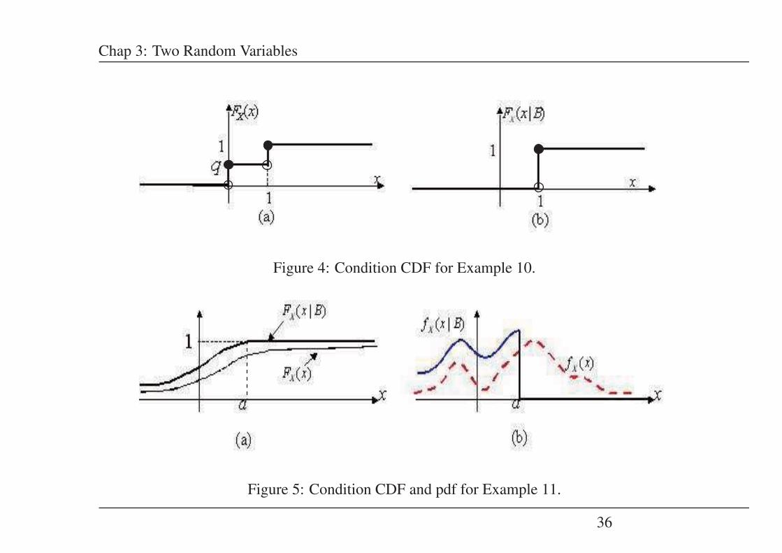
Example 10: Toss a coin and X(T ) = 0, X(H) = 1. Suppose B = {H}. Determine
FX(x|B). (Suppose q is the probability of landing a tail)
Solution: From earlier example, FX(x) has the following form shown in Fig. 4(a). We needFX(x|B) for all x.
• For x < 0, {X(ξ) ≤ x} = φ, so that {(X(ξ) ≤ x) ∩ B} = φ and FX(x|B) = 0.
• For 0 ≤ x < 1, {X(ξ) ≤ x} = {T}, so that
{(X(ξ) ≤ x) ∩ B} = {T} ∩ {H} = φ
and FX(x|B) = 0.
• For x ≥ 1, {X(ξ) ≤ x} = Ω, and
{(X(ξ) ≤ x) ∩ B} = Ω ∩ {B} = {B}and
FX(x|B) =P (B)P (B)
= 1
The conditional CDF is shown in Fig. 4(b).
35
Chap 3: Two Random Variables
Figure 4: Condition CDF for Example 10.
Figure 5: Condition CDF and pdf for Example 11.
36
Chap 3: Two Random Variables
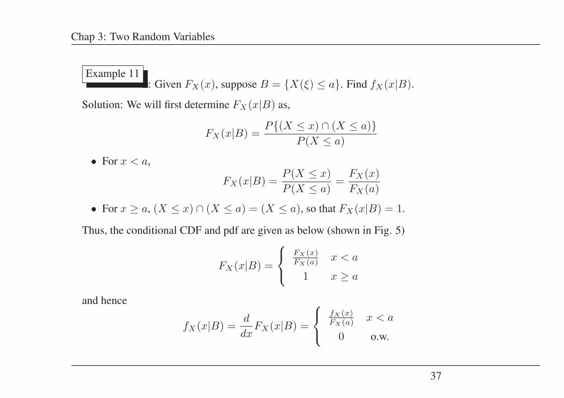
Example 11: Given FX(x), suppose B = {X(ξ) ≤ a}. Find fX(x|B).
Solution: We will first determine FX(x|B) as,
FX(x|B) =P{(X ≤ x) ∩ (X ≤ a)}
P (X ≤ a)
• For x < a,
FX(x|B) =P (X ≤ x)P (X ≤ a)
=FX(x)FX(a)
• For x ≥ a, (X ≤ x) ∩ (X ≤ a) = (X ≤ a), so that FX(x|B) = 1.
Thus, the conditional CDF and pdf are given as below (shown in Fig. 5)
FX(x|B) =
⎧⎨⎩
FX(x)FX(a) x < a
1 x ≥ a
and hence
fX(x|B) =d
dxFX(x|B) =
⎧⎨⎩
fX(x)FX(a) x < a
0 o.w.
37
Chap 3: Two Random Variables
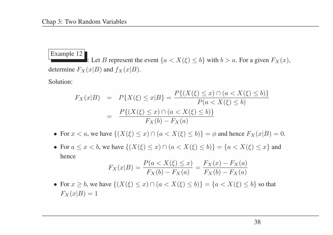
Example 12: Let B represent the event {a < X(ξ) ≤ b} with b > a. For a given FX(x),
determine FX(x|B) and fX(x|B).
Solution:
FX(x|B) = P{X(ξ) ≤ x|B} =P{(X(ξ) ≤ x) ∩ (a < X(ξ) ≤ b)}
P (a < X(ξ) ≤ b)
=P{(X(ξ) ≤ x) ∩ (a < X(ξ) ≤ b)}
FX(b) − FX(a)
• For x < a, we have {(X(ξ) ≤ x) ∩ (a < X(ξ) ≤ b)} = φ and hence FX(x|B) = 0.
• For a ≤ x < b, we have {(X(ξ) ≤ x) ∩ (a < X(ξ) ≤ b)} = {a < X(ξ) ≤ x} andhence
FX(x|B) =P (a < X(ξ) ≤ x)FX(b) − FX(a)
=FX(x) − FX(a)FX(b) − FX(a)
• For x ≥ b, we have {(X(ξ) ≤ x) ∩ (a < X(ξ) ≤ b)} = {a < X(ξ) ≤ b} so thatFX(x|B) = 1
38

Chap 3: Two Random Variables
Therefore, the density function shown below and given as
fX(x|B) =
⎧⎨⎩
fX(x)FX(b)−FX(a) a < x ≤ b
0 o.w.
Figure 6: Condition pdf for Example 12.
39
Chap 3: Two Random Variables
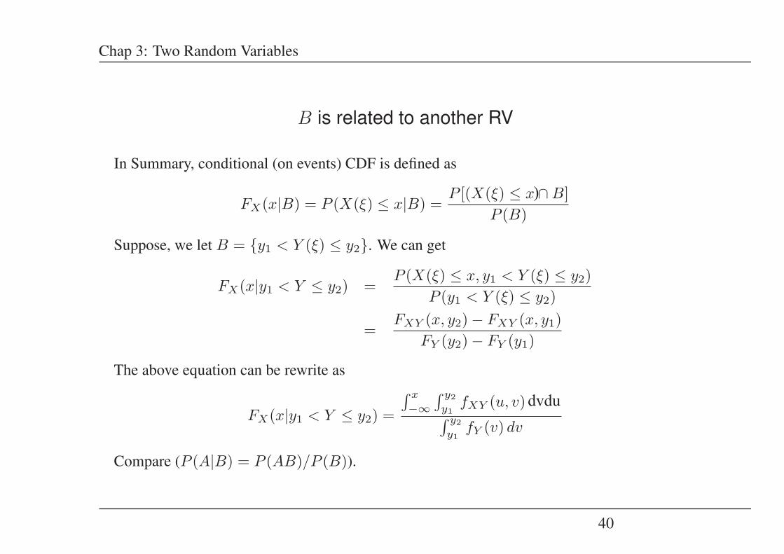
B is related to another RV
In Summary, conditional (on events) CDF is defined as
FX(x|B) = P (X(ξ) ≤ x|B) =P [(X(ξ) ≤ x ∩ B]
P (B)
Suppose, we let B = {y1 < Y (ξ) ≤ y2}. We can get
FX(x|y1 < Y ≤ y2) =P (X(ξ) ≤ x, y1 < Y (ξ) ≤ y2)
P (y1 < Y (ξ) ≤ y2)
=FXY (x, y2) − FXY (x, y1)
FY (y2) − FY (y1)
The above equation can be rewrite as
FX(x|y1 < Y ≤ y2) =
∫ x
−∞∫ y2
y1fXY (u, v) dudv∫ y2
y1fY (v) dv
Compare (P (A|B) = P (AB)/P (B)).
40
)
dvdu

Chap 3: Two Random Variables
We have examined how to condition a mass/density function by the occurrence of an eventB, where event B describes some property of X . Now we focus on the special case in whichthe event B has the form of X = x or Y = y. Learning Y = y changes the likelihood thatX = x. For example, conditional PMF is defined as:
PX|Y (x|y) = P [X = x|Y = y]
To determine, the limiting case FX(x|Y = y), we can let y1 = y and y2 = y + Δy, then thisgives
FX(x|y < Y ≤ y + Δy) =
∫ x
−∞∫ y+Δy
yfXY (u, v) dudv∫ y+Δy
yfY (v) dv
=
∫ x
−∞ fXY (u, v) duΔy
fY (y)Δy
and hence in the limit
FX(x|Y = y) = limΔy→0
FX(x|y < Y ≤ y + Δy) =
∫ x
−∞ fXY (u, v) du
fY (y)
To remind about the conditional nature on the left hand side, we shall use the subscript X|Y
41
dvdu
Chap 3: Two Random Variables
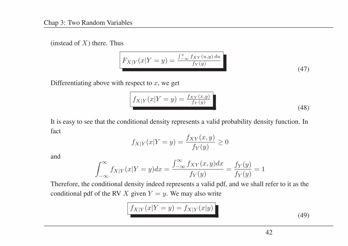
(instead of X) there. Thus
FX|Y (x|Y = y) =∫ x−∞ fXY (u,y) du
fY (y)
(47)
Differentiating above with respect to x, we get
fX|Y (x|Y = y) = fXY (x,y)fY (y)
(48)
It is easy to see that the conditional density represents a valid probability density function. Infact
fX|Y (x|Y = y) =fXY (x, y)
fY (y)≥ 0
and ∫ ∞
−∞fX|Y (x|Y = y)dx =
∫∞−∞ fXY (x, y)dx
fY (y)=
fY (y)fY (y)
= 1
Therefore, the conditional density indeed represents a valid pdf, and we shall refer to it as theconditional pdf of the RV X given Y = y. We may also write
fX|Y (x|Y = y) = fX|Y (x|y)(49)
42
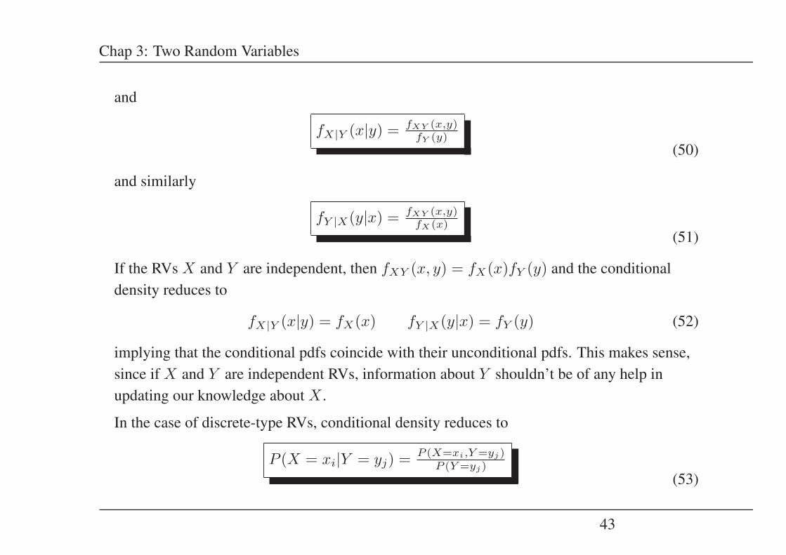
Chap 3: Two Random Variables
and
fX|Y (x|y) = fXY (x,y)fY (y)
(50)
and similarly
fY |X(y|x) = fXY (x,y)fX(x)
(51)
If the RVs X and Y are independent, then fXY (x, y) = fX(x)fY (y) and the conditionaldensity reduces to
fX|Y (x|y) = fX(x) fY |X(y|x) = fY (y) (52)
implying that the conditional pdfs coincide with their unconditional pdfs. This makes sense,since if X and Y are independent RVs, information about Y shouldn’t be of any help inupdating our knowledge about X .
In the case of discrete-type RVs, conditional density reduces to
P (X = xi|Y = yj) = P (X=xi,Y =yj)P (Y =yj)
(53)
43
Chap 3: Two Random Variables
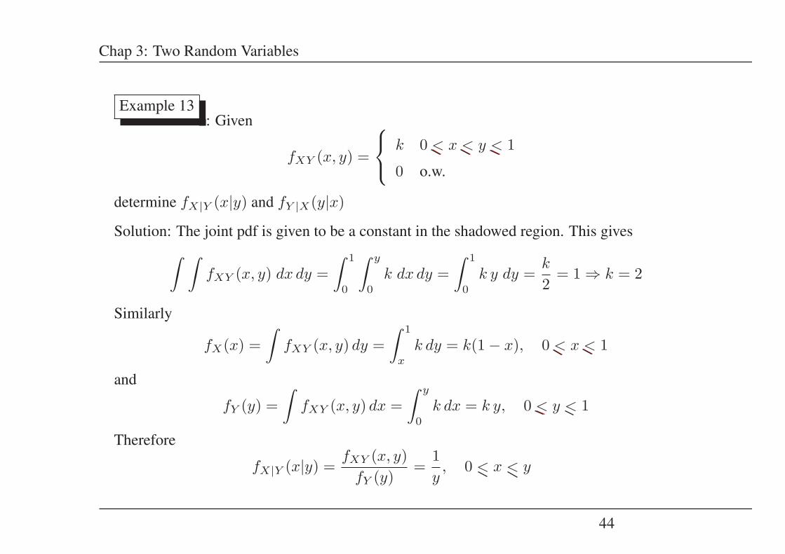
Example 13: Given
fXY (x, y) =
⎧⎨⎩ k 0 < x < y < 1
0 o.w.
determine fX|Y (x|y) and fY |X(y|x)
Solution: The joint pdf is given to be a constant in the shadowed region. This gives∫ ∫fXY (x, y) dx dy =
∫ 1
0
∫ y
0
k dx dy =∫ 1
0
k y dy =k
2= 1 ⇒ k = 2
Similarly
fX(x) =∫
fXY (x, y) dy =∫ 1
x
k dy = k(1 − x), 0 < x < 1
and
fY (y) =∫
fXY (x, y) dx =∫ y
0
k dx = k y, 0 < y < 1
Therefore
fX|Y (x|y) =fXY (x, y)
fY (y)=
1y, 0 < x < y < 1
44

Chap 3: Two Random Variables
and
fY |X(y|x) =fXY (x, y)
fX(x)=
11 − x
, 0 < x < y < 1
Figure 7: Joint pdf of X and Y (Example 13).
45
Chap 3: Two Random Variables
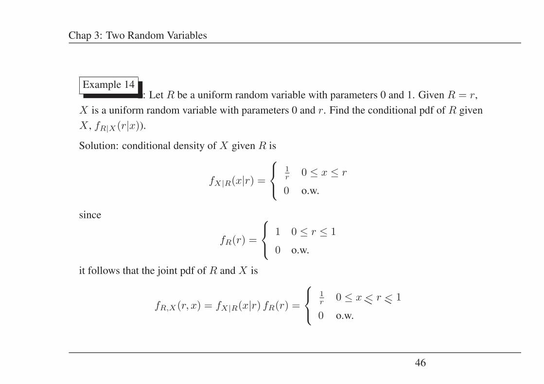
Example 14: Let R be a uniform random variable with parameters 0 and 1. Given R = r,
X is a uniform random variable with parameters 0 and r. Find the conditional pdf of R givenX , fR|X(r|x)).
Solution: conditional density of X given R is
fX|R(x|r) =
⎧⎨⎩
1r 0 ≤ x ≤ r
0 o.w.
since
fR(r) =
⎧⎨⎩ 1 0 ≤ r ≤ 1
0 o.w.
it follows that the joint pdf of R and X is
fR,X(r, x) = fX|R(x|r) fR(r) =
⎧⎨⎩
1r 0 ≤ x < r < 1
0 o.w.
46
Chap 3: Two Random Variables
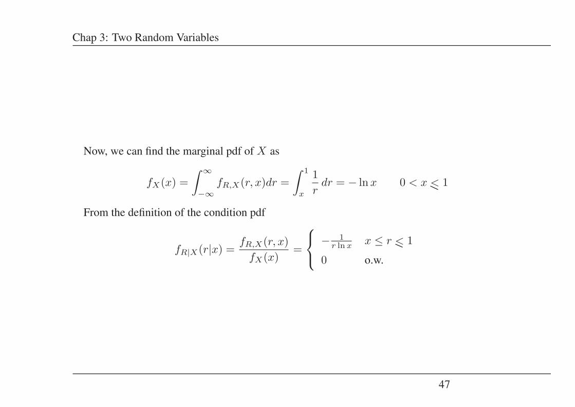
Now, we can find the marginal pdf of X as
fX(x) =∫ ∞
−∞fR,X(r, x)dr =
∫ 1
x
1r
dr = − lnx 0 < x < 1
From the definition of the condition pdf
fR|X(r|x) =fR,X(r, x)
fX(x)=
⎧⎨⎩ − 1
r ln x x ≤ r < 1
0 o.w.
47

Chap 3: Two Random Variables
Chap 3.5 : Conditional Mean
We can use the conditional pdfs to define the conditional mean. More generally, applyingdefinition of expectation to conditional pdfs we get
E[g(X)|B] =∫ ∞
−∞g(x)fX(x|B) dx
Using a limiting argument, we obtain
μX|Y = E(X|Y = y) =∫∞−∞ xfX|Y (x|y) dx
(54)
to be the conditional mean of X given Y = y. Notice that E(X|Y = y) will be a function ofy. Also
μY |X = E(Y |X = x) =∫∞−∞ yfY |X(y|x) dy
(55)
In a similar manner, the conditional variance of X given Y = y is given by
V ar(X|Y ) = σ2X|Y = E(X2|Y = y) − [E(X|Y = y)]2 = E[(x − μX|Y )2|Y = y]
(56)
48
Chap 3: Two Random Variables
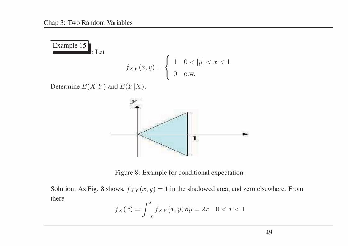
Example 15: Let
fXY (x, y) =
⎧⎨⎩ 1 0 < |y| < x < 1
0 o.w.
Determine E(X|Y ) and E(Y |X).
Figure 8: Example for conditional expectation.
Solution: As Fig. 8 shows, fXY (x, y) = 1 in the shadowed area, and zero elsewhere. Fromthere
fX(x) =∫ x
−x
fXY (x, y) dy = 2x 0 < x < 1
49

Chap 3: Two Random Variables
and
fY (y) =∫ 1
|y|1 dx = 1 − |y| |y| < 1
This gives
fX|Y (x|y) =fXY (x, y)
fY (y)=
11 − |y| 0 < |y| < x < 1
and
fY |X(y|x) =fXY (x, y)
fX(x)=
12x
0 < |y| < x < 1
Hence
E(X|Y ) =∫
xfX|Y (x|y) dx =∫ 1
|y|
x
1 − |y| dx =1
1 − |y|x2
2
∣∣∣∣1
|y|
=1 − |y|2
2(1 − |y|) =1 + |y|
2|y| < 1
E(Y |X) =∫
y fY |X(y|x) dy =∫ x
−x
y
2xdy =
12x
y2
2
∣∣∣∣x
−x
= 0 0 < x < 1
50
Chap 3: Two Random Variables
It is possible to obtain an interesting generalization of the conditional mean formulas as
E[g(X)|Y = y)] =∫ ∞
−∞g(x)fX|Y (x|y) dx (57)
51

Chap 3: Two Random Variables
Example 16: Poisson sum of Bernoulli random variables: Let Xi, i = 1, 2, 3, · · · ,
represent independent, identically distributed Bernoulli random variables with
P (Xi = 1) = p P (Xi = 0) = 1 − p = q
and N a Poisson random variable with parameter λ that is independent of all Xi. Considerthe random variables
Y1 =N∑
i=1
Xi, Y2 = N − Y1
Show that Y1 and Y2 are independent Poisson random variables.
Solution : the joint probability mass function of Y1 and Y2 can be solved as
P (Y1 = m,Y2 = n) = P (Y1 = m,N − Y1 = n) = P (Y1 = m,N = m + n)
= P (Y1 = m|N = m + n)P (N = m + n)
= P
(N∑
i=1
Xi = m|N = m + n
)P (N = m + n)
= P
(m+n∑i=1
Xi = m
)P (N = m + n)
52
Chap 3: Two Random Variables
Note that∑m+n
i=1 Xi ∼ B(m + n, p) and Xi’s are independent of N
P (Y1 = m,Y2 = n) =(
(m + n)!m!n!
pm qn
)(e−λ λm+n
(m + n)!
)
=(
e−pλ (pλ)m
m!
)(e−qλ (qλ)n
n!
)= P (Y1 = m) · P (Y2 = n)
Thus,Y1 ∼ P (pλ) Y2 ∼ P (qλ)
and Y1 and Y2 are independent random variables. Thus if a bird lays eggs that follow aPoisson random variable with parameter λ, and if each egg survives with probability p, thenthe number of baby birds that survive also forms a Poisson random variable with parameterpλ.
Example 17: Suppose that the number of people who visit a yoga academy each day is a
Poisson RV. with mean λ. Suppose further that each person who visits is, independently,female with probability p or male with probability 1 − p. Find the joint probability that
53
Chap 3: Two Random Variables
exactly n women and m men visit the academy today.
Solution: Let N1 denote the number of women, and N2 the number of men, who visit theacademy today. Also, let N = N1 + N2 be the total number of people who visit.Conditioning on N gives
P (N1 = n,N2 = m) =∞∑
i=0
P [N1 = n,N2 = m|N = i]P (N = i)
Because P [N1 = n,N2 = m|N = i] = 0 when n + m = i, therefore
P (N1 = n,N2 = m) = P [N1 = n,N2 = m|N = n + m]e−λ λn+m
(n + m)!
=
⎛⎝ n + m
n
⎞⎠ pn(1 − p)me−λ λn+m
(n + m)!
= e−λp (λp)n
n!× e−λ(1−p) [λ(1 − p)]m
m!= P (N1 = n) × P (N2 = m) (58)
We can conclude that N1 and N2 are independent Poisson RVs with respectively means λp
and λ(1 − p). Therefore, example 16 and 17 showed an important result: when each of a
54

Chap 3: Two Random Variables
Poisson number of events is independently classified either as being type 1 with probability p
or type 2 with probability 1 − p, then the number of type 1 and type 2 events are independentPoisson random variables.
55
Chap 3: Two Random Variables
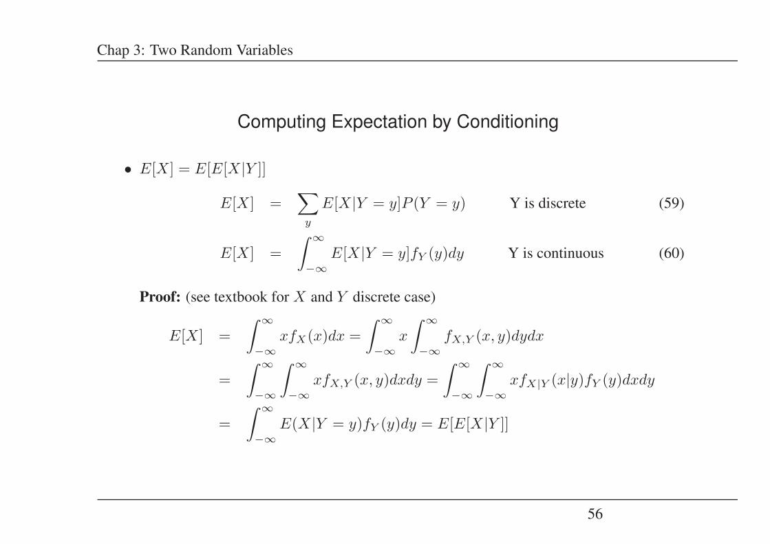
Computing Expectation by Conditioning
• E[X] = E[E[X|Y ]]
E[X] =∑
y
E[X|Y = y]P (Y = y) Y is discrete (59)
E[X] =∫ ∞
−∞E[X|Y = y]fY (y)dy Y is continuous (60)
Proof: (see textbook for X and Y discrete case)
E[X] =∫ ∞
−∞xfX(x)dx =
∫ ∞
−∞x
∫ ∞
−∞fX,Y (x, y)dydx
=∫ ∞
−∞
∫ ∞
−∞xfX,Y (x, y)dxdy =
∫ ∞
−∞
∫ ∞
−∞xfX|Y (x|y)fY (y)dxdy
=∫ ∞
−∞E(X|Y = y)fY (y)dy = E[E[X|Y ]]
56
Chap 3: Two Random Variables
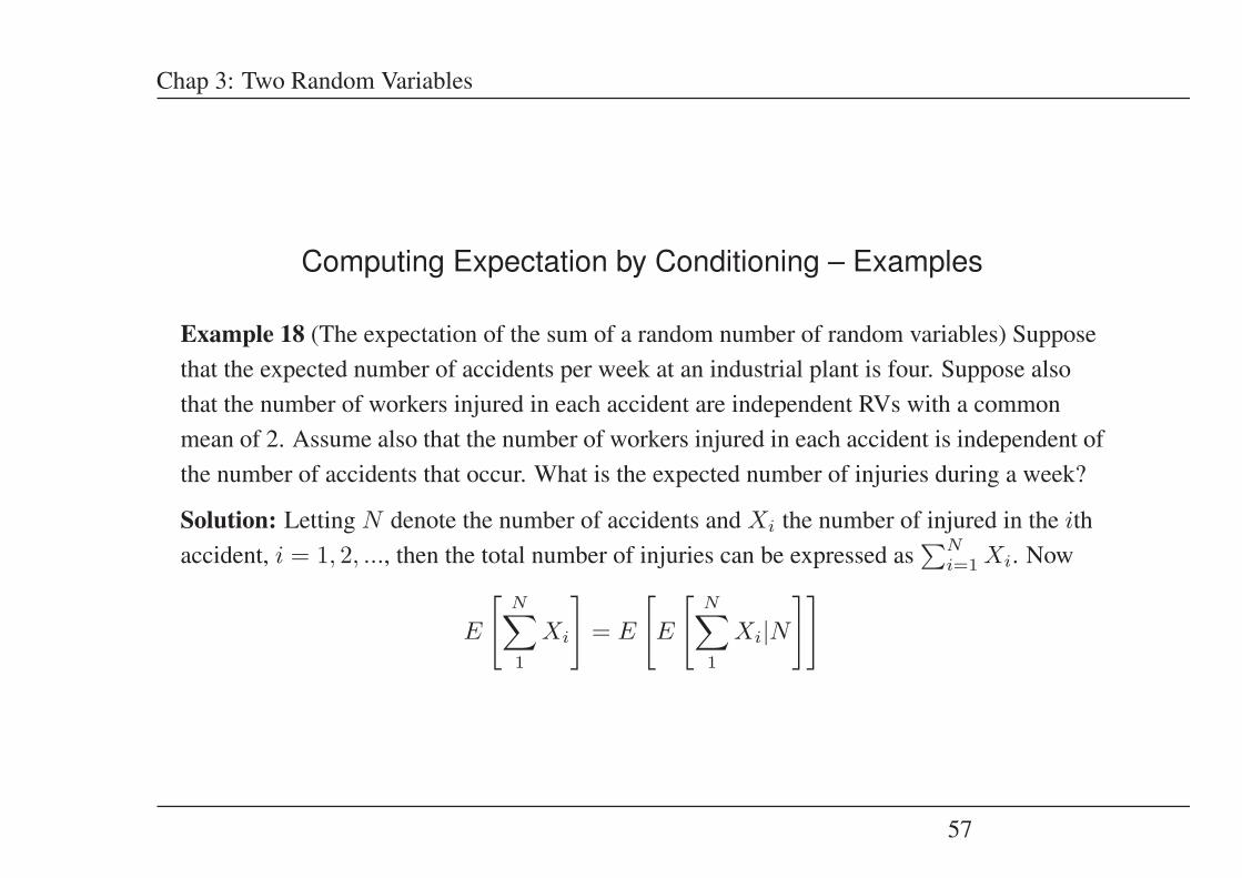
Computing Expectation by Conditioning – Examples
Example 18 (The expectation of the sum of a random number of random variables) Supposethat the expected number of accidents per week at an industrial plant is four. Suppose alsothat the number of workers injured in each accident are independent RVs with a commonmean of 2. Assume also that the number of workers injured in each accident is independent ofthe number of accidents that occur. What is the expected number of injuries during a week?
Solution: Letting N denote the number of accidents and Xi the number of injured in the ithaccident, i = 1, 2, ..., then the total number of injuries can be expressed as
∑Ni=1 Xi. Now
E
[N∑1
Xi
]= E
[E
[N∑1
Xi|N]]
57

Chap 3: Two Random Variables
But
E
[N∑1
Xi|N = n
]= E
[n∑1
Xi|N = n
]
= E
[n∑1
Xi
]by independence of Xi and N
= nE[X]
which is
E
[N∑1
Xi|N]
= NE[X]
and thus
E
[N∑1
Xi
]= E[NE[X]] = E[N ]E[X]
Therefore, the expected number of injuries during a week equals 4 × 2 = 8.
58
Chap 3: Two Random Variables
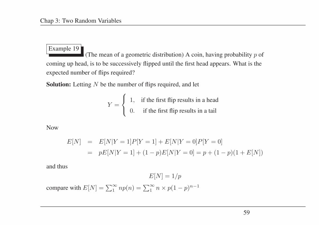
Example 19(The mean of a geometric distribution) A coin, having probability p of
coming up head, is to be successively flipped until the first head appears. What is theexpected number of flips required?
Solution: Letting N be the number of flips required, and let
Y =
⎧⎨⎩ 1, if the first flip results in a head
0. if the first flip results in a tail
Now
E[N ] = E[N |Y = 1]P [Y = 1] + E[N |Y = 0]P [Y = 0]
= pE[N |Y = 1] + (1 − p)E[N |Y = 0] = p + (1 − p)(1 + E[N ])
and thusE[N ] = 1/p
compare with E[N ] =∑∞
1 np(n) =∑∞
1 n × p(1 − p)n−1
59
Chap 3: Two Random Variables
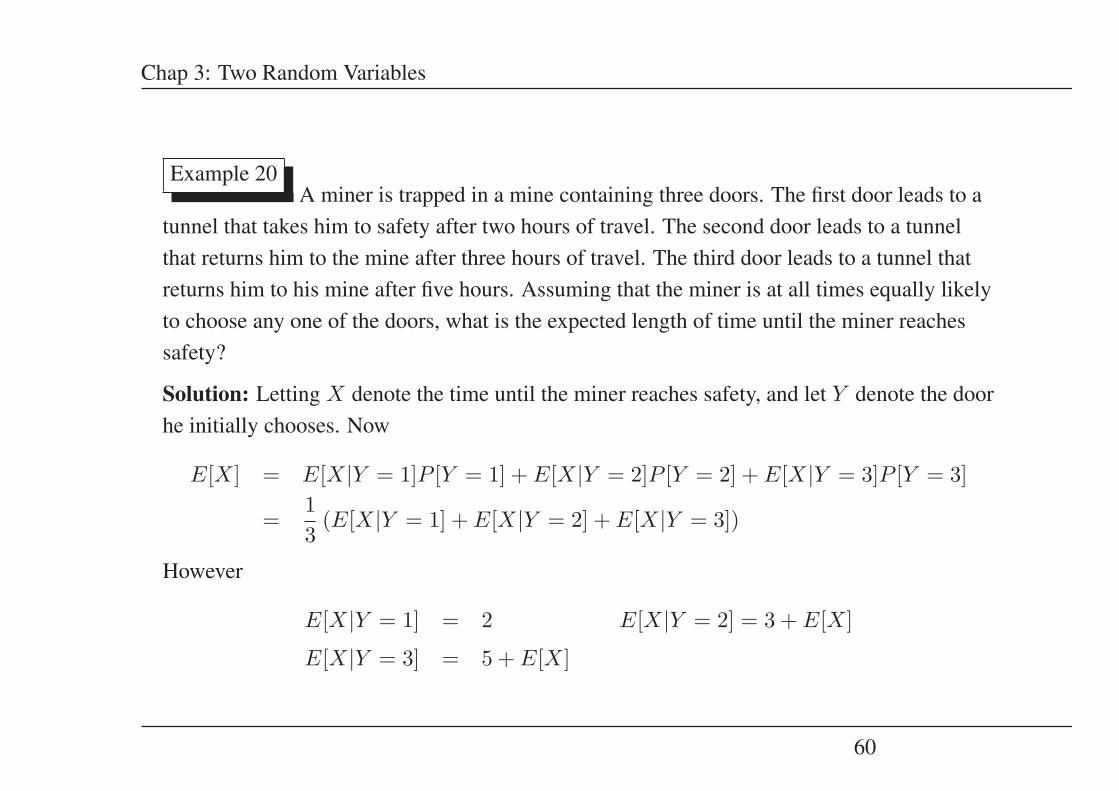
Example 20A miner is trapped in a mine containing three doors. The first door leads to a
tunnel that takes him to safety after two hours of travel. The second door leads to a tunnelthat returns him to the mine after three hours of travel. The third door leads to a tunnel thatreturns him to his mine after five hours. Assuming that the miner is at all times equally likelyto choose any one of the doors, what is the expected length of time until the miner reachessafety?
Solution: Letting X denote the time until the miner reaches safety, and let Y denote the doorhe initially chooses. Now
E[X] = E[X|Y = 1]P [Y = 1] + E[X|Y = 2]P [Y = 2] + E[X|Y = 3]P [Y = 3]
=13
(E[X|Y = 1] + E[X|Y = 2] + E[X|Y = 3])
However
E[X|Y = 1] = 2 E[X|Y = 2] = 3 + E[X]
E[X|Y = 3] = 5 + E[X]
60
Chap 3: Two Random Variables
and thus
E[X] =13(2 + 3 + E[X] + 5 + E[X]) leads to E[X] = 10 hours.
61

Chap 3: Two Random Variables
Computing Probability by Conditioning
Let E denote an arbitary event and define the indicator RV. X by
X =
⎧⎨⎩ 1, if E occurs
0, if E does not occur
It follows thatE[X] = P [E] and E[X|Y = y] = P [E|Y = y]
for any RV Y . Therefore,
P [E] =∑
y
P [E|Y = y]P (Y = y) if Y is discrete (61)
=∫ ∞
−∞P [E|Y = y]fY (y)dy if Y is continuous (62)
62
,
Chap 3: Two Random Variables
Example 21Suppose that X and Y are independent continuous random variables having
densities fX and fY , respectively. Compute P (X < Y )
Solution: Conditioning on the value of Y yields
P (X < Y ) =∫ ∞
−∞P [X < Y |Y = y]fY (y)dy
=∫ ∞
−∞P [X < y|Y = y]fY (y)dy
=∫ ∞
−∞P (X < y)fY (y)dy
=∫ ∞
−∞FX(y)fY (y)dy
where
FX(y) =∫ y
−∞fX(x)dx
63