chap09
DESCRIPTION
TRANSCRIPT
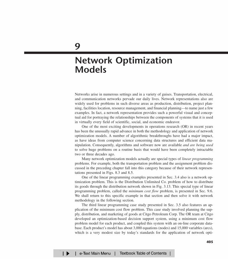
405
9Network Optimization Models
Networks arise in numerous settings and in a variety of guises. Transportation, electrical,and communication networks pervade our daily lives. Network representations also arewidely used for problems in such diverse areas as production, distribution, project plan-ning, facilities location, resource management, and financial planning—to name just a fewexamples. In fact, a network representation provides such a powerful visual and concep-tual aid for portraying the relationships between the components of systems that it is usedin virtually every field of scientific, social, and economic endeavor.
One of the most exciting developments in operations research (OR) in recent yearshas been the unusually rapid advance in both the methodology and application of networkoptimization models. A number of algorithmic breakthroughs have had a major impact,as have ideas from computer science concerning data structures and efficient data ma-nipulation. Consequently, algorithms and software now are available and are being usedto solve huge problems on a routine basis that would have been completely intractabletwo or three decades ago.
Many network optimization models actually are special types of linear programmingproblems. For example, both the transportation problem and the assignment problem dis-cussed in the preceding chapter fall into this category because of their network represen-tations presented in Figs. 8.3 and 8.5.
One of the linear programming examples presented in Sec. 3.4 also is a network op-timization problem. This is the Distribution Unlimited Co. problem of how to distributeits goods through the distribution network shown in Fig. 3.13. This special type of linearprogramming problem, called the minimum cost flow problem, is presented in Sec. 9.6.We shall return to this specific example in that section and then solve it with networkmethodology in the following section.
The third linear programming case study presented in Sec. 3.5 also features an ap-plication of the minimum cost flow problem. This case study involved planning the sup-ply, distribution, and marketing of goods at Citgo Petroleum Corp. The OR team at Citgodeveloped an optimization-based decision support system, using a minimum cost flowproblem model for each product, and coupled this system with an on-line corporate data-base. Each product’s model has about 3,000 equations (nodes) and 15,000 variables (arcs),which is a very modest size by today’s standards for the application of network opti-

mization models. The model takes in all aspects of the business, helping management de-cide everything from run levels at the various refineries to what prices to pay or charge.A network representation is essential because of the flow of goods through several stages:purchase of crude oil from various suppliers, shipping it to refineries, refining it into var-ious products, and sending the products to distribution centers and product storage ter-minals for subsequent sale. As discussed in Sec. 3.5, the modeling system enabled thecompany to reduce its petroleum products inventory by over $116 million with no dropin service levels. This resulted in a savings in annual interest of $14 million as well asimprovements in coordination, pricing, and purchasing decisions worth another $2.5 mil-lion each year, along with many indirect benefits.
In this one chapter we only scratch the surface of the current state of the art of net-work methodology. However, we shall introduce you to four important kinds of networkproblems and some basic ideas of how to solve them (without delving into issues of datastructures that are so vital to successful large-scale implementations). Each of the first threeproblem types—the shortest-path problem, the minimum spanning tree problem, and themaximum flow problem—has a very specific structure that arises frequently in applications.
The fourth type—the minimum cost flow problem—provides a unified approach tomany other applications because of its far more general structure. In fact, this structure isso general that it includes as special cases both the shortest-path problem and the maxi-mum flow problem as well as the transportation problem and the assignment problemfrom Chap. 8. Because the minimum cost flow problem is a special type of linear pro-gramming problem, it can be solved extremely efficiently by a streamlined version of thesimplex method called the network simplex method. (We shall not discuss even more gen-eral network problems that are more difficult to solve.)
The first section introduces a prototype example that will be used subsequently to il-lustrate the approach to the first three of these problems. Section 9.2 presents some basicterminology for networks. The next four sections deal with the four problems in turn. Sec-tion 9.7 then is devoted to the network simplex method.
406 9 NETWORK OPTIMIZATION MODELS
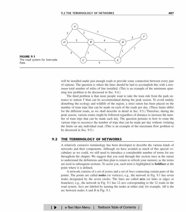
SEERVADA PARK has recently been set aside for a limited amount of sightseeing andbackpack hiking. Cars are not allowed into the park, but there is a narrow, winding roadsystem for trams and for jeeps driven by the park rangers. This road system is shown(without the curves) in Fig. 9.1, where location O is the entrance into the park; other let-ters designate the locations of ranger stations (and other limited facilities). The numbersgive the distances of these winding roads in miles.
The park contains a scenic wonder at station T. A small number of trams are used totransport sightseers from the park entrance to station T and back.
The park management currently faces three problems. One is to determine which routefrom the park entrance to station T has the smallest total distance for the operation of thetrams. (This is an example of the shortest-path problem to be discussed in Sec. 9.3.)
A second problem is that telephone lines must be installed under the roads to estab-lish telephone communication among all the stations (including the park entrance). Be-cause the installation is both expensive and disruptive to the natural environment, lines
9.1 PROTOTYPE EXAMPLE
will be installed under just enough roads to provide some connection between every pairof stations. The question is where the lines should be laid to accomplish this with a min-imum total number of miles of line installed. (This is an example of the minimum span-ning tree problem to be discussed in Sec. 9.4.)
The third problem is that more people want to take the tram ride from the park en-trance to station T than can be accommodated during the peak season. To avoid undulydisturbing the ecology and wildlife of the region, a strict ration has been placed on thenumber of tram trips that can be made on each of the roads per day. (These limits differfor the different roads, as we shall describe in detail in Sec. 9.5.) Therefore, during thepeak season, various routes might be followed regardless of distance to increase the num-ber of tram trips that can be made each day. The question pertains to how to route thevarious trips to maximize the number of trips that can be made per day without violatingthe limits on any individual road. (This is an example of the maximum flow problem tobe discussed in Sec. 9.5.)
9.2 THE TERMINOLOGY OF NETWORKS 407
O
C E
D
T
B
A
5
17
7
4
2
31
4
2
5
4FIGURE 9.1The road system for SeervadaPark.
A relatively extensive terminology has been developed to describe the various kinds ofnetworks and their components. Although we have avoided as much of this special vo-cabulary as we could, we still need to introduce a considerable number of terms for usethroughout the chapter. We suggest that you read through this section once at the outsetto understand the definitions and then plan to return to refresh your memory as the termsare used in subsequent sections. To assist you, each term is highlighted in boldface at thepoint where it is defined.
A network consists of a set of points and a set of lines connecting certain pairs of thepoints. The points are called nodes (or vertices); e.g., the network in Fig. 9.1 has sevennodes designated by the seven circles. The lines are called arcs (or links or edges orbranches); e.g., the network in Fig. 9.1 has 12 arcs corresponding to the 12 roads in theroad system. Arcs are labeled by naming the nodes at either end; for example, AB is thearc between nodes A and B in Fig. 9.1.
9.2 THE TERMINOLOGY OF NETWORKS
The arcs of a network may have a flow of some type through them, e.g., the flow oftrams on the roads of Seervada Park in Sec. 9.1. Table 9.1 gives several examples of flowin typical networks. If flow through an arc is allowed in only one direction (e.g., a one-way street), the arc is said to be a directed arc. The direction is indicated by adding anarrowhead at the end of the line representing the arc. When a directed arc is labeled bylisting two nodes it connects, the from node always is given before the to node; e.g., anarc that is directed from node A to node B must be labeled as AB rather than BA. Alter-natively, this arc may be labeled as A � B.
If flow through an arc is allowed in either direction (e.g., a pipeline that can be usedto pump fluid in either direction), the arc is said to be an undirected arc. To help youdistinguish between the two kinds of arcs, we shall frequently refer to undirected arcs bythe suggestive name of links.
Although the flow through an undirected arc is allowed to be in either direction, we doassume that the flow will be one way in the direction of choice rather than having simulta-neous flows in opposite directions. (The latter case requires the use of a pair of directedarcs in opposite directions.) However, in the process of making the decision on the flowthrough an undirected arc, it is permissible to make a sequence of assignments of flows inopposite directions, but with the understanding that the actual flow will be the net flow (thedifference of the assigned flows in the two directions). For example, if a flow of 10 has beenassigned in one direction and then a flow of 4 is assigned in the opposite direction, the ac-tual effect is to cancel 4 units of the original assignment by reducing the flow in the origi-nal direction from 10 to 6. Even for a directed arc, the same technique sometimes is usedas a convenient device to reduce a previously assigned flow. In particular, you are allowedto make a fictional assignment of flow in the “wrong” direction through a directed arc torecord a reduction of that amount in the flow in the “right” direction.
A network that has only directed arcs is called a directed network. Similarly, if allits arcs are undirected, the network is said to be an undirected network. A network witha mixture of directed and undirected arcs (or even all undirected arcs) can be convertedto a directed network, if desired, by replacing each undirected arc by a pair of directedarcs in opposite directions. (You then have the choice of interpreting the flows througheach pair of directed arcs as being simultaneous flows in opposite directions or providinga net flow in one direction, depending on which fits your application.)
When two nodes are not connected by an arc, a natural question is whether they areconnected by a series of arcs. A path between two nodes is a sequence of distinct arcsconnecting these nodes. For example, one of the paths connecting nodes O and T in Fig.9.1 is the sequence of arcs OB–BD–DT (O � B � D � T), or vice versa. When some
408 9 NETWORK OPTIMIZATION MODELS
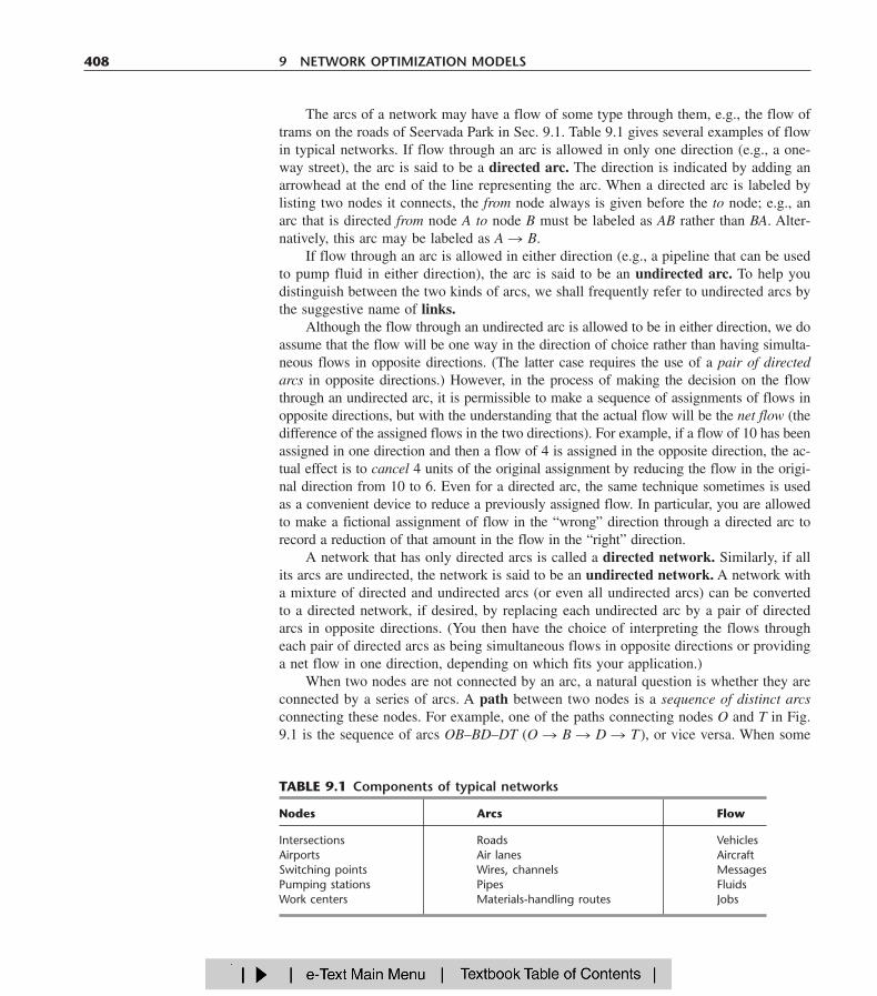
TABLE 9.1 Components of typical networks
Nodes Arcs Flow
Intersections Roads VehiclesAirports Air lanes AircraftSwitching points Wires, channels MessagesPumping stations Pipes FluidsWork centers Materials-handling routes Jobs
of or all the arcs in the network are directed arcs, we then distinguish between directedpaths and undirected paths. A directed path from node i to node j is a sequence of con-necting arcs whose direction (if any) is toward node j, so that flow from node i to node jalong this path is feasible. An undirected path from node i to node j is a sequence ofconnecting arcs whose direction (if any) can be either toward or away from node j. (No-tice that a directed path also satisfies the definition of an undirected path, but not viceversa.) Frequently, an undirected path will have some arcs directed toward node j but oth-ers directed away (i.e., toward node i). You will see in Secs. 9.5 and 9.7 that, perhaps sur-prisingly, undirected paths play a major role in the analysis of directed networks.
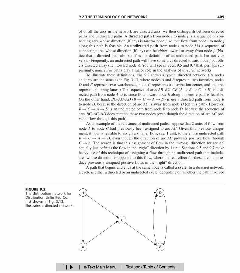
To illustrate these definitions, Fig. 9.2 shows a typical directed network. (Its nodesand arcs are the same as in Fig. 3.13, where nodes A and B represent two factories, nodesD and E represent two warehouses, node C represents a distribution center, and the arcsrepresent shipping lanes.) The sequence of arcs AB–BC–CE (A � B � C � E) is a di-rected path from node A to E, since flow toward node E along this entire path is feasible.On the other hand, BC–AC–AD (B � C � A � D) is not a directed path from node Bto node D, because the direction of arc AC is away from node D (on this path). However,B � C � A � D is an undirected path from node B to node D, because the sequence ofarcs BC–AC–AD does connect these two nodes (even though the direction of arc AC pre-vents flow through this path).
As an example of the relevance of undirected paths, suppose that 2 units of flow fromnode A to node C had previously been assigned to arc AC. Given this previous assign-ment, it now is feasible to assign a smaller flow, say, 1 unit, to the entire undirected pathB � C � A � D, even though the direction of arc AC prevents positive flow through C � A. The reason is that this assignment of flow in the “wrong” direction for arc ACactually just reduces the flow in the “right” direction by 1 unit. Sections 9.5 and 9.7 makeheavy use of this technique of assigning a flow through an undirected path that includesarcs whose direction is opposite to this flow, where the real effect for these arcs is to re-duce previously assigned positive flows in the “right” direction.
A path that begins and ends at the same node is called a cycle. In a directed network,a cycle is either a directed or an undirected cycle, depending on whether the path involved
9.2 THE TERMINOLOGY OF NETWORKS 409
A
B E
D
C
FIGURE 9.2The distribution network forDistribution Unlimited Co.,first shown in Fig. 3.13,illustrates a directed network.
is a directed or an undirected path. (Since a directed path also is an undirected path, a di-rected cycle is an undirected cycle, but not vice versa in general.) In Fig. 9.2, for exam-ple, DE–ED is a directed cycle. By contrast, AB–BC–AC is not a directed cycle, becausethe direction of arc AC opposes the direction of arcs AB and BC. On the other hand,AB–BC–AC is an undirected cycle, because A � B � C � A is an undirected path. Inthe undirected network shown in Fig. 9.1, there are many cycles, for example,OA–AB–BC–CO. However, note that the definition of path (a sequence of distinct arcs)rules out retracing one’s steps in forming a cycle. For example, OB–BO in Fig. 9.1 doesnot qualify as a cycle, because OB and BO are two labels for the same arc (link). On theother hand, DE–ED is a (directed) cycle in Fig. 9.2, because DE and ED are distinct arcs.
Two nodes are said to be connected if the network contains at least one undirectedpath between them. (Note that the path does not need to be directed even if the networkis directed.) A connected network is a network where every pair of nodes is connected.Thus, the networks in Figs. 9.1 and 9.2 are both connected. However, the latter networkwould not be connected if arcs AD and CE were removed.
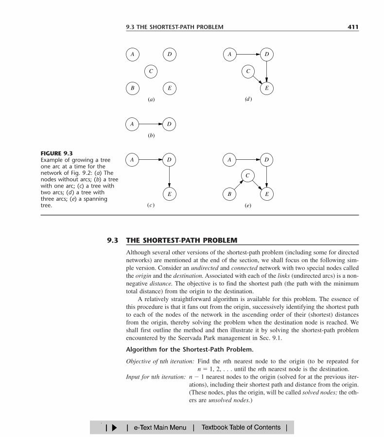
Consider a connected network with n nodes (e.g., the n � 5 nodes in Fig. 9.2) whereall the arcs have been deleted. A “tree” can then be “grown” by adding one arc (or “branch”)at a time from the original network in a certain way. The first arc can go anywhere to con-nect some pair of nodes. Thereafter, each new arc should be between a node that alreadyis connected to other nodes and a new node not previously connected to any other nodes.Adding an arc in this way avoids creating a cycle and ensures that the number of con-nected nodes is 1 greater than the number of arcs. Each new arc creates a larger tree,which is a connected network (for some subset of the n nodes) that contains no undirectedcycles. Once the (n � 1)st arc has been added, the process stops because the resulting treespans (connects) all n nodes. This tree is called a spanning tree, i.e., a connected net-work for all n nodes that contains no undirected cycles. Every spanning tree has exactlyn � 1 arcs, since this is the minimum number of arcs needed to have a connected networkand the maximum number possible without having undirected cycles.
Figure 9.3 uses the five nodes and some of the arcs of Fig. 9.2 to illustrate this processof growing a tree one arc (branch) at a time until a spanning tree has been obtained. Thereare several alternative choices for the new arc at each stage of the process, so Fig. 9.3shows only one of many ways to construct a spanning tree in this case. Note, however,how each new added arc satisfies the conditions specified in the preceding paragraph. Weshall discuss and illustrate spanning trees further in Sec. 9.4.
Spanning trees play a key role in the analysis of many networks. For example, theyform the basis for the minimum spanning tree problem discussed in Sec. 9.4. Anotherprime example is that (feasible) spanning trees correspond to the BF solutions for the net-work simplex method discussed in Sec. 9.7.
Finally, we shall need a little additional terminology about flows in networks. Themaximum amount of flow (possibly infinity) that can be carried on a directed arc is re-ferred to as the arc capacity. For nodes, a distinction is made among those that are netgenerators of flow, net absorbers of flow, or neither. A supply node (or source node orsource) has the property that the flow out of the node exceeds the flow into the node. Thereverse case is a demand node (or sink node or sink), where the flow into the node ex-ceeds the flow out of the node. A transshipment node (or intermediate node) satisfiesconservation of flow, so flow in equals flow out.
410 9 NETWORK OPTIMIZATION MODELS
9.3 THE SHORTEST-PATH PROBLEM 411
A
B
D
C
E
(a)
(b)
A
B
D
C
E
A D
A D
E
(e)(c )
A D
C
E
(d )
FIGURE 9.3Example of growing a treeone arc at a time for thenetwork of Fig. 9.2: (a) Thenodes without arcs; (b) a treewith one arc; (c) a tree withtwo arcs; (d) a tree withthree arcs; (e) a spanningtree.
Although several other versions of the shortest-path problem (including some for directednetworks) are mentioned at the end of the section, we shall focus on the following sim-ple version. Consider an undirected and connected network with two special nodes calledthe origin and the destination. Associated with each of the links (undirected arcs) is a non-negative distance. The objective is to find the shortest path (the path with the minimumtotal distance) from the origin to the destination.
A relatively straightforward algorithm is available for this problem. The essence ofthis procedure is that it fans out from the origin, successively identifying the shortest pathto each of the nodes of the network in the ascending order of their (shortest) distancesfrom the origin, thereby solving the problem when the destination node is reached. Weshall first outline the method and then illustrate it by solving the shortest-path problemencountered by the Seervada Park management in Sec. 9.1.
Algorithm for the Shortest-Path Problem.
Objective of nth iteration: Find the nth nearest node to the origin (to be repeated for n � 1, 2, . . . until the nth nearest node is the destination.
Input for nth iteration: n � 1 nearest nodes to the origin (solved for at the previous iter-ations), including their shortest path and distance from the origin.(These nodes, plus the origin, will be called solved nodes; the oth-ers are unsolved nodes.)
9.3 THE SHORTEST-PATH PROBLEM
Candidates for nth nearest node: Each solved node that is directly connected by a linkto one or more unsolved nodes provides one candi-date—the unsolved node with the shortest connectinglink. (Ties provide additional candidates.)
Calculation of nth nearest node: For each such solved node and its candidate, add thedistance between them and the distance of the shortestpath from the origin to this solved node. The candidatewith the smallest such total distance is the nth nearestnode (ties provide additional solved nodes), and itsshortest path is the one generating this distance.
Applying This Algorithm to the Seervada Park Shortest-Path Problem
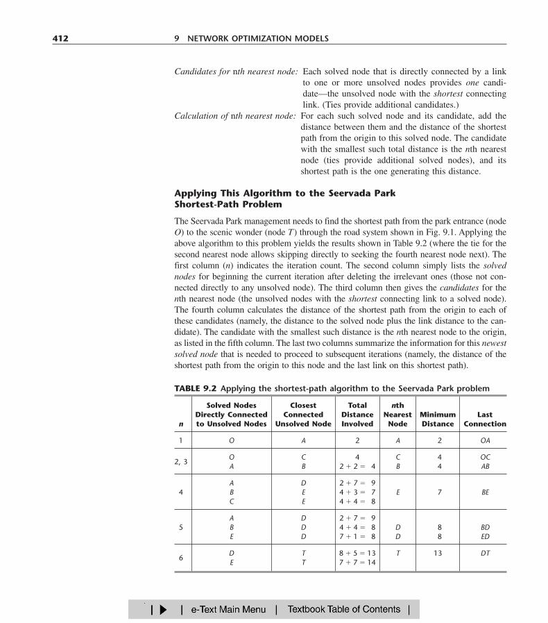
The Seervada Park management needs to find the shortest path from the park entrance (nodeO) to the scenic wonder (node T) through the road system shown in Fig. 9.1. Applying theabove algorithm to this problem yields the results shown in Table 9.2 (where the tie for thesecond nearest node allows skipping directly to seeking the fourth nearest node next). Thefirst column (n) indicates the iteration count. The second column simply lists the solvednodes for beginning the current iteration after deleting the irrelevant ones (those not con-nected directly to any unsolved node). The third column then gives the candidates for thenth nearest node (the unsolved nodes with the shortest connecting link to a solved node).The fourth column calculates the distance of the shortest path from the origin to each ofthese candidates (namely, the distance to the solved node plus the link distance to the can-didate). The candidate with the smallest such distance is the nth nearest node to the origin,as listed in the fifth column. The last two columns summarize the information for this newestsolved node that is needed to proceed to subsequent iterations (namely, the distance of theshortest path from the origin to this node and the last link on this shortest path).
412 9 NETWORK OPTIMIZATION MODELS
TABLE 9.2 Applying the shortest-path algorithm to the Seervada Park problem
Solved Nodes Closest Total nthDirectly Connected Connected Distance Nearest Minimum Last
n to Unsolved Nodes Unsolved Node Involved Node Distance Connection
1 O A 2 A 2 OA
O C 4 C 4 OC2, 3
A B 2 � 2 � 4 B 4 AB
A D 2 � 7 � 94 B E 4 � 3 � 7 E 7 BE
C E 4 � 4 � 8
A D 2 � 7 � 95 B D 4 � 4 � 8 D 8 BD
E D 7 � 1 � 8 D 8 ED
D T 8 � 5 � 13 T 13 DT6
E T 7 � 7 � 14
Now let us relate these columns directly to the outline given for the algorithm. Theinput for nth iteration is provided by the fifth and sixth columns for the preceding itera-tions, where the solved nodes in the fifth column are then listed in the second column forthe current iteration after deleting those that are no longer directly connected to unsolvednodes. The candidates for nth nearest node next are listed in the third column for the cur-rent iteration. The calculation of nth nearest node is performed in the fourth column, andthe results are recorded in the last three columns for the current iteration.
After the work shown in Table 9.2 is completed, the shortest path from the destinationto the origin can be traced back through the last column of Table 9.2 as eitherT � D � E � B � A � O or T � D � B � A � O. Therefore, the two alternates forthe shortest path from the origin to the destination have been identified as O � A � B �E � D � T and O � A � B � D � T, with a total distance of 13 miles on either path.
Using Excel to Formulate and Solve Shortest-Path Problems
This algorithm provides a particularly efficient way of solving large shortest-path prob-lems. However, some mathematical programming software packages do not include thisalgorithm. If not, they often will include the network simplex method described in Sec.9.7, which is another good option for these problems.
Since the shortest-path problem is a special type of linear programming problem, thegeneral simplex method also can be used when better options are not readily available. Al-though not nearly as efficient as these specialized algorithms on large shortest-path problems,it is quite adequate for problems of even very substantial size (much larger than the SeervadaPark problem). Excel, which relies on the general simplex method, provides a convenientway of formulating and solving shortest-path problems with dozens of arcs and nodes.
Figure 9.4 shows an appropriate spreadsheet formulation for the Seervada Park short-est-path problem. Rather than using the kind of formulation presented in Sec. 3.6 that usesa separate row for each functional constraint of the linear programming model, this for-mulation exploits the special structure by listing the nodes in column G and the arcs incolumns B and C, as well as the distance (in miles) along each arc in column E. Sinceeach link in the network is an undirected arc, whereas travel through the shortest path isin one direction, each link can be replaced by a pair of directed arcs in opposite direc-tions. Thus, columns B and C together list both of the nearly vertical links in Fig. 9.1 (A–B and D–E) twice, once as a downward arc and once as an upward arc, since eitherdirection might be on the chosen path. However, the other links are only listed as left-to-right arcs, since this is the only direction of interest for choosing a shortest path from theorigin to the destination.
A trip from the origin to the destination is interpreted to be a “flow” of 1 on the cho-sen path through the network. The decisions to be made are which arcs should be includedin the path to be traversed. A flow of 1 is assigned to an arc if it is included, whereas theflow is 0 if it is not included. Thus, the decision variables are
xij � �for each of the arcs under consideration. The values of these decision variables are en-tered in the changing cells in column D (cells D4:D17).
if arc i � j is not includedif arc i � j is included
01
9.3 THE SHORTEST-PATH PROBLEM 413
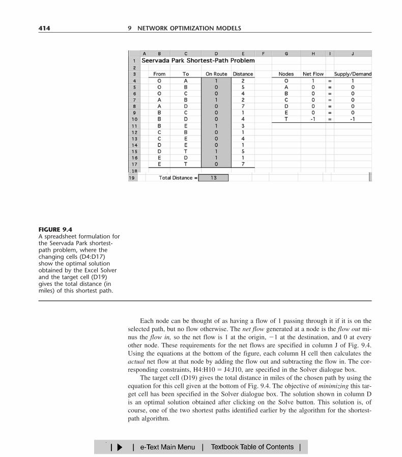
Each node can be thought of as having a flow of 1 passing through it if it is on theselected path, but no flow otherwise. The net flow generated at a node is the flow out mi-nus the flow in, so the net flow is 1 at the origin, �1 at the destination, and 0 at everyother node. These requirements for the net flows are specified in column J of Fig. 9.4.Using the equations at the bottom of the figure, each column H cell then calculates theactual net flow at that node by adding the flow out and subtracting the flow in. The cor-responding constraints, H4:H10 � J4:J10, are specified in the Solver dialogue box.
The target cell (D19) gives the total distance in miles of the chosen path by using theequation for this cell given at the bottom of Fig. 9.4. The objective of minimizing this tar-get cell has been specified in the Solver dialogue box. The solution shown in column Dis an optimal solution obtained after clicking on the Solve button. This solution is, ofcourse, one of the two shortest paths identified earlier by the algorithm for the shortest-path algorithm.
414 9 NETWORK OPTIMIZATION MODELS
FIGURE 9.4A spreadsheet formulation forthe Seervada Park shortest-path problem, where thechanging cells (D4:D17)show the optimal solutionobtained by the Excel Solverand the target cell (D19)gives the total distance (inmiles) of this shortest path.
Other Applications
Not all applications of the shortest-path problem involve minimizing the distance traveledfrom the origin to the destination. In fact, they might not even involve travel at all. Thelinks (or arcs) might instead represent activities of some other kind, so choosing a paththrough the network corresponds to selecting the best sequence of activities. The numbersgiving the “lengths” of the links might then be, for example, the costs of the activities, inwhich case the objective would be to determine which sequence of activities minimizesthe total cost.
Here are three categories of applications.
1. Minimize the total distance traveled, as in the Seervada Park example.2. Minimize the total cost of a sequence of activities. (Problem 9.3-2 is of this type.)3. Minimize the total time of a sequence of activities. (Problems 9.3-5 and 9.3-6 are of
this type.)
It is even possible for all three categories to arise in the same application. For example, sup-pose you wish to find the best route for driving from one town to another through a num-ber of intermediate towns. You then have the choice of defining the best route as being theone that minimizes the total distance traveled or that minimizes the total cost incurred orthat minimizes the total time required. (Problem 9.3-1 illustrates such an application.)
Many applications require finding the shortest directed path from the origin to thedestination through a directed network. The algorithm already presented can be easilymodified to deal just with directed paths at each iteration. In particular, when candidatesfor the nth nearest node are identified, only directed arcs from a solved node to an un-solved node are considered.
Another version of the shortest-path problem is to find the shortest paths from theorigin to all the other nodes of the network. Notice that the algorithm already solves forthe shortest path to each node that is closer to the origin than the destination. Therefore,when all nodes are potential destinations, the only modification needed in the algorithmis that it does not stop until all nodes are solved nodes.
An even more general version of the shortest-path problem is to find the shortest pathsfrom every node to every other node. Another option is to drop the restriction that “dis-tances” (arc values) be nonnegative. Constraints also can be imposed on the paths that canbe followed. All these variations occasionally arise in applications and so have been stud-ied by researchers.
The algorithms for a wide variety of combinatorial optimization problems, such as cer-tain vehicle routing or network design problems, often call for the solution of a large num-ber of shortest-path problems as subroutines. Although we lack the space to pursue thistopic further, this use may now be the most important kind of application of the shortest-path problem.
9.4 THE MINIMUM SPANNING TREE PROBLEM 415
The minimum spanning tree problem bears some similarities to the main version of theshortest-path problem presented in the preceding section. In both cases, an undirected andconnected network is being considered, where the given information includes some mea-sure of the positive length (distance, cost, time, etc.) associated with each link. Both prob-
9.4 THE MINIMUM SPANNING TREE PROBLEM
lems also involve choosing a set of links that have the shortest total length among all setsof links that satisfy a certain property. For the shortest-path problem, this property is thatthe chosen links must provide a path between the origin and the destination. For the min-imum spanning tree problem, the required property is that the chosen links must providea path between each pair of nodes.
The minimum spanning tree problem can be summarized as follows.
1. You are given the nodes of a network but not the links. Instead, you are given the po-tential links and the positive length for each if it is inserted into the network. (Alter-native measures for the length of a link include distance, cost, and time.)
2. You wish to design the network by inserting enough links to satisfy the requirementthat there be a path between every pair of nodes.
3. The objective is to satisfy this requirement in a way that minimizes the total length ofthe links inserted into the network.
A network with n nodes requires only (n � 1) links to provide a path between each pairof nodes. No extra links should be used, since this would needlessly increase the total lengthof the chosen links. The (n � 1) links need to be chosen in such a way that the resultingnetwork (with just the chosen links) forms a spanning tree (as defined in Sec. 9.2). There-fore, the problem is to find the spanning tree with a minimum total length of the links.
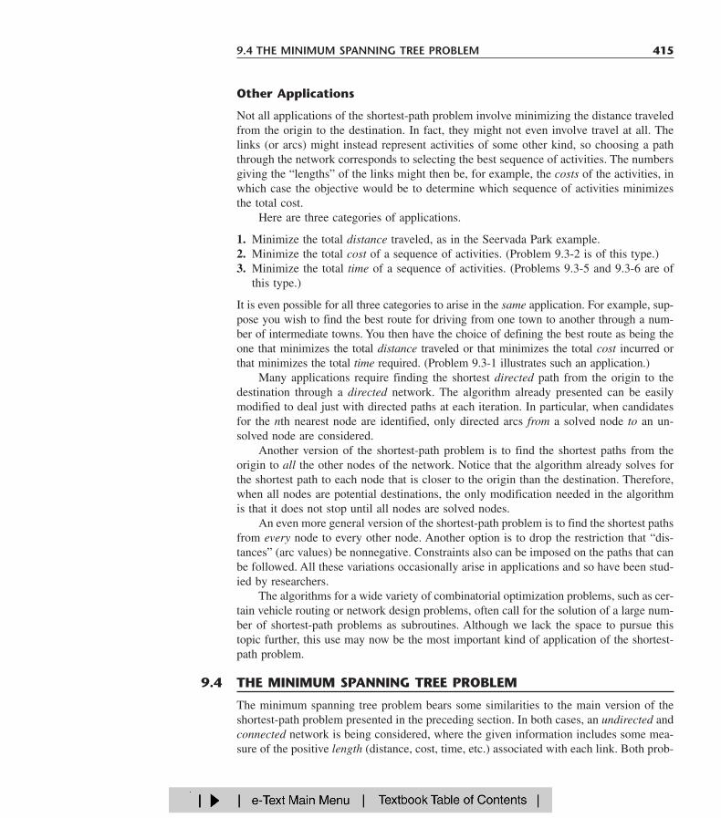
Figure 9.5 illustrates this concept of a spanning tree for the Seervada Park problem(see Sec. 9.1). Thus, Fig. 9.5a is not a spanning tree because nodes O, A, B, and C arenot connected with nodes D, E, and T. It needs another link to make this connection. Thisnetwork actually consists of two trees, one for each of these two sets of nodes. The linksin Fig. 9.5b do span the network (i.e., the network is connected as defined in Sec. 9.2),but it is not a tree because there are two cycles (O–A–B–C–O and D–T–E–D). It has toomany links. Because the Seervada Park problem has n � 7 nodes, Sec. 9.2 indicates thatthe network must have exactly n � 1 � 6 links, with no cycles, to qualify as a spanningtree. This condition is achieved in Fig. 9.5c, so this network is a feasible solution (with avalue of 24 miles for the total length of the links) for the minimum spanning tree prob-lem. (You soon will see that this solution is not optimal because it is possible to constructa spanning tree with only 14 miles of links.)
Some Applications
Here is a list of some key types of applications of the minimum spanning tree problem.
1. Design of telecommunication networks (fiber-optic networks, computer networks,leased-line telephone networks, cable television networks, etc.)
2. Design of a lightly used transportation network to minimize the total cost of provid-ing the links (rail lines, roads, etc.)
3. Design of a network of high-voltage electrical power transmission lines4. Design of a network of wiring on electrical equipment (e.g., a digital computer sys-
tem) to minimize the total length of the wire5. Design of a network of pipelines to connect a number of locations
In this age of the information superhighway, applications of this first type have be-come particularly important. In a telecommunication network, it is only necessary to in-
416 9 NETWORK OPTIMIZATION MODELS
sert enough links to provide a path between every pair of nodes, so designing such a net-work is a classic application of the minimum spanning tree problem. Because sometelecommunication networks now cost many millions of dollars, it is very important tooptimize their design by finding the minimum spanning tree for each one.
An Algorithm
The minimum spanning tree problem can be solved in a very straightforward way becauseit happens to be one of the few OR problems where being greedy at each stage of the so-lution procedure still leads to an overall optimal solution at the end! Thus, beginning withany node, the first stage involves choosing the shortest possible link to another node, with-out worrying about the effect of this choice on subsequent decisions. The second stageinvolves identifying the unconnected node that is closest to either of these connected nodesand then adding the corresponding link to the network. This process is repeated, per thefollowing summary, until all the nodes have been connected. (Note that this is the sameprocess already illustrated in Fig. 9.3 for constructing a spanning tree, but now with a spe-cific rule for selecting each new link.) The resulting network is guaranteed to be a mini-mum spanning tree.
9.4 THE MINIMUM SPANNING TREE PROBLEM 417
O
C E
D
T
B
A
(a)
O
C E
D
T
B
A
(b)
O
C E
D
T
B
A
5
7
22
4
(c)
4FIGURE 9.5Illustrations of the spanningtree concept for theSeervada Park problem: (a) Not a spanning tree; (b) not a spanning tree; (c) a spanning tree.
Algorithm for the Minimum Spanning Tree Problem.
1. Select any node arbitrarily, and then connect it (i.e., add a link) to the nearest distinct node.2. Identify the unconnected node that is closest to a connected node, and then connect
these two nodes (i.e., add a link between them). Repeat this step until all nodes havebeen connected.
3. Tie breaking: Ties for the nearest distinct node (step 1) or the closest unconnected node(step 2) may be broken arbitrarily, and the algorithm must still yield an optimal solu-tion. However, such ties are a signal that there may be (but need not be) multiple op-timal solutions. All such optimal solutions can be identified by pursuing all ways ofbreaking ties to their conclusion.
The fastest way of executing this algorithm manually is the graphical approach il-lustrated next.
Applying This Algorithm to the Seervada Park Minimum Spanning Tree Problem
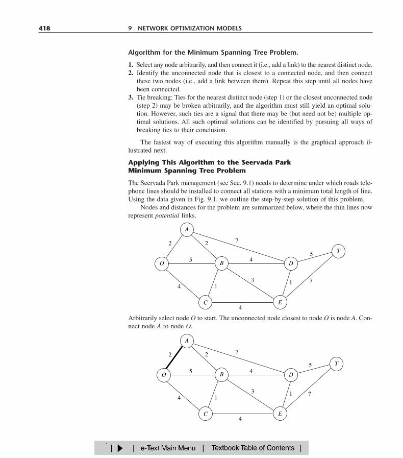
The Seervada Park management (see Sec. 9.1) needs to determine under which roads tele-phone lines should be installed to connect all stations with a minimum total length of line.Using the data given in Fig. 9.1, we outline the step-by-step solution of this problem.
Nodes and distances for the problem are summarized below, where the thin lines nowrepresent potential links.
418 9 NETWORK OPTIMIZATION MODELS
O
C E
D
T
B
A
5
1 7
7
4
2
31
4
2
5
4
C E
D
T
B
5
1 7
7
4
2
31
4
2
5
4
A
O
Arbitrarily select node O to start. The unconnected node closest to node O is node A. Con-nect node A to node O.

The unconnected node closest to either node O or node A is node B (closest to A). Con-nect node B to node A.
9.4 THE MINIMUM SPANNING TREE PROBLEM 419
The unconnected node closest to node O, A, or B is node C (closest to B). Connect nodeC to node B.
The unconnected node closest to node O, A, B, or C is node E (closest to B). Connectnode E to node B.
C E
D
T5
1 7
7
4
2
31
4
2
5
4
O
A
B
E
D
T5
1 7
7
4
2
31
4
2
5
4
O
C
B
A
D
T5
1 7
7
4
2
31
4
2
5
4
O
C E
B
A
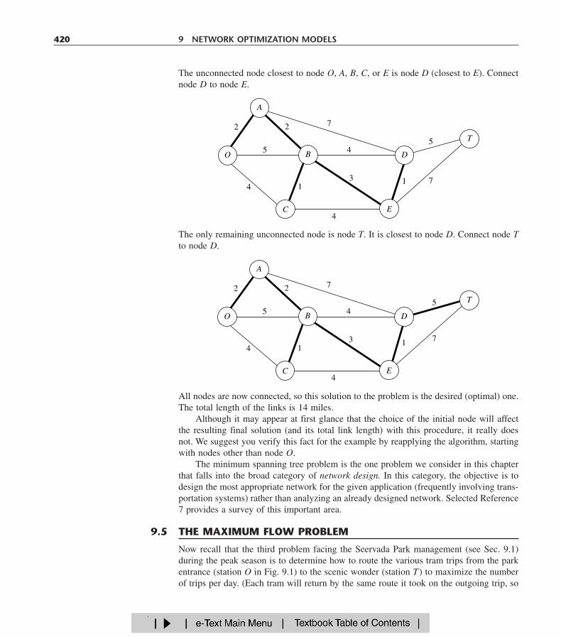
The unconnected node closest to node O, A, B, C, or E is node D (closest to E). Connectnode D to node E.
420 9 NETWORK OPTIMIZATION MODELS
The only remaining unconnected node is node T. It is closest to node D. Connect node Tto node D.
All nodes are now connected, so this solution to the problem is the desired (optimal) one.The total length of the links is 14 miles.
Although it may appear at first glance that the choice of the initial node will affectthe resulting final solution (and its total link length) with this procedure, it really doesnot. We suggest you verify this fact for the example by reapplying the algorithm, startingwith nodes other than node O.
The minimum spanning tree problem is the one problem we consider in this chapterthat falls into the broad category of network design. In this category, the objective is todesign the most appropriate network for the given application (frequently involving trans-portation systems) rather than analyzing an already designed network. Selected Reference7 provides a survey of this important area.
T5
1 7
7
4
2
31
4
2
5
4
BO
C
D
E
A
T5
1 7
7
4
2
31
4
2
5
4
O
C
A
E
DB
Now recall that the third problem facing the Seervada Park management (see Sec. 9.1)during the peak season is to determine how to route the various tram trips from the parkentrance (station O in Fig. 9.1) to the scenic wonder (station T) to maximize the numberof trips per day. (Each tram will return by the same route it took on the outgoing trip, so
9.5 THE MAXIMUM FLOW PROBLEM
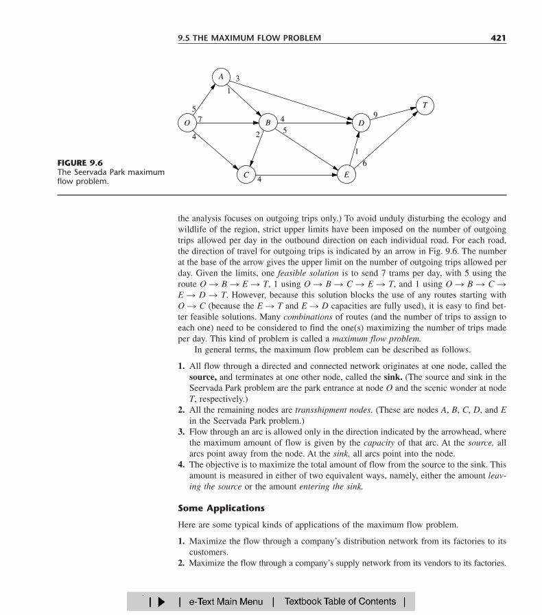
the analysis focuses on outgoing trips only.) To avoid unduly disturbing the ecology andwildlife of the region, strict upper limits have been imposed on the number of outgoingtrips allowed per day in the outbound direction on each individual road. For each road,the direction of travel for outgoing trips is indicated by an arrow in Fig. 9.6. The numberat the base of the arrow gives the upper limit on the number of outgoing trips allowed perday. Given the limits, one feasible solution is to send 7 trams per day, with 5 using theroute O � B � E � T, 1 using O � B � C � E � T, and 1 using O � B � C �E � D � T. However, because this solution blocks the use of any routes starting with O � C (because the E � T and E � D capacities are fully used), it is easy to find bet-ter feasible solutions. Many combinations of routes (and the number of trips to assign toeach one) need to be considered to find the one(s) maximizing the number of trips madeper day. This kind of problem is called a maximum flow problem.
In general terms, the maximum flow problem can be described as follows.
1. All flow through a directed and connected network originates at one node, called thesource, and terminates at one other node, called the sink. (The source and sink in theSeervada Park problem are the park entrance at node O and the scenic wonder at nodeT, respectively.)
2. All the remaining nodes are transshipment nodes. (These are nodes A, B, C, D, and Ein the Seervada Park problem.)
3. Flow through an arc is allowed only in the direction indicated by the arrowhead, wherethe maximum amount of flow is given by the capacity of that arc. At the source, allarcs point away from the node. At the sink, all arcs point into the node.
4. The objective is to maximize the total amount of flow from the source to the sink. Thisamount is measured in either of two equivalent ways, namely, either the amount leav-ing the source or the amount entering the sink.
Some Applications
Here are some typical kinds of applications of the maximum flow problem.
1. Maximize the flow through a company’s distribution network from its factories to itscustomers.
2. Maximize the flow through a company’s supply network from its vendors to its factories.
9.5 THE MAXIMUM FLOW PROBLEM 421
O
C E
DB
A
9
1
6
3
4
2 5
1
4
57
4
T
FIGURE 9.6The Seervada Park maximumflow problem.

3. Maximize the flow of oil through a system of pipelines.4. Maximize the flow of water through a system of aqueducts.5. Maximize the flow of vehicles through a transportation network.
For some of these applications, the flow through the network may originate at morethan one node and may also terminate at more than one node, even though a maximumflow problem is allowed to have only a single source and a single sink. For example, acompany’s distribution network commonly has multiple factories and multiple customers.A clever reformulation is used to make such a situation fit the maximum flow problem.This reformulation involves expanding the original network to include a dummy source,a dummy sink, and some new arcs. The dummy source is treated as the node that origi-nates all the flow that, in reality, originates from some of the other nodes. For each ofthese other nodes, a new arc is inserted that leads from the dummy source to this node,where the capacity of this arc equals the maximum flow that, in reality, can originate fromthis node. Similarly, the dummy sink is treated as the node that absorbs all the flow that,in reality, terminates at some of the other nodes. Therefore, a new arc is inserted fromeach of these other nodes to the dummy sink, where the capacity of this arc equals themaximum flow that, in reality, can terminate at this node. Because of all these changes,all the nodes in the original network now are transshipment nodes, so the expanded net-work has the required single source (the dummy source) and single sink (the dummy sink)to fit the maximum flow problem.
An Algorithm
Because the maximum flow problem can be formulated as a linear programming prob-lem (see Prob. 9.5-2), it can be solved by the simplex method, so any of the linear pro-gramming software packages introduced in Chaps. 3 and 4 can be used. However, an evenmore efficient augmenting path algorithm is available for solving this problem. This al-gorithm is based on two intuitive concepts, a residual network and an augmenting path.
After some flows have been assigned to the arcs, the residual network shows the re-maining arc capacities (called residual capacities) for assigning additional flows. For ex-ample, consider arc O � B in Fig. 9.6, which has an arc capacity of 7. Now suppose thatthe assigned flows include a flow of 5 through this arc, which leaves a residual capacityof 7 � 5 � 2 for any additional flow assignment through O � B. This status is depictedas follows in the residual network.
422 9 NETWORK OPTIMIZATION MODELS
The number on an arc next to a node gives the residual capacity for flow from that nodeto the other node. Therefore, in addition to the residual capacity of 2 for flow from O toB, the 5 on the right indicates a residual capacity of 5 for assigning some flow from B toO (that is, for canceling some previously assigned flow from O to B).
Initially, before any flows have been assigned, the residual network for the SeervadaPark problem has the appearance shown in Fig. 9.7. Every arc in the original network(Fig. 9.6) has been changed from a directed arc to an undirected arc. However, the arc
5O B
2

capacity in the original direction remains the same and the arc capacity in the oppositedirection is zero, so the constraints on flows are unchanged.
Subsequently, whenever some amount of flow is assigned to an arc, that amount issubtracted from the residual capacity in the same direction and added to the residual ca-pacity in the opposite direction.
An augmenting path is a directed path from the source to the sink in the residualnetwork such that every arc on this path has strictly positive residual capacity. The mini-mum of these residual capacities is called the residual capacity of the augmenting pathbecause it represents the amount of flow that can feasibly be added to the entire path.Therefore, each augmenting path provides an opportunity to further augment the flowthrough the original network.
The augmenting path algorithm repeatedly selects some augmenting path and adds aflow equal to its residual capacity to that path in the original network. This process con-tinues until there are no more augmenting paths, so the flow from the source to the sinkcannot be increased further. The key to ensuring that the final solution necessarily is op-timal is the fact that augmenting paths can cancel some previously assigned flows in theoriginal network, so an indiscriminate selection of paths for assigning flows cannot pre-vent the use of a better combination of flow assignments.
To summarize, each iteration of the algorithm consists of the following three steps.
The Augmenting Path Algorithm for the Maximum Flow Problem.1
1. Identify an augmenting path by finding some directed path from the source to the sinkin the residual network such that every arc on this path has strictly positive residualcapacity. (If no augmenting path exists, the net flows already assigned constitute anoptimal flow pattern.)
2. Identify the residual capacity c* of this augmenting path by finding the minimum ofthe residual capacities of the arcs on this path. Increase the flow in this path by c*.
3. Decrease by c* the residual capacity of each arc on this augmenting path. Increase byc* the residual capacity of each arc in the opposite direction on this augmenting path.Return to step 1.
9.5 THE MAXIMUM FLOW PROBLEM 423
O
C E
T
B9
16
4
1
52
4
0
7
4
3
0
5
0
00
0
0
000
0
0
D
A
FIGURE 9.7The initial residual networkfor the Seervada Parkmaximum flow problem.
1It is assumed that the arc capacities are either integers or rational numbers.
When step 1 is carried out, there often will be a number of alternative augmentingpaths from which to choose. Although the algorithmic strategy for making this selectionis important for the efficiency of large-scale implementations, we shall not delve into thisrelatively specialized topic. (Later in the section, we do describe a systematic procedurefor finding some augmenting path.) Therefore, for the following example (and the prob-lems at the end of the chapter), the selection is just made arbitrarily.
Applying This Algorithm to the Seervada Park Maximum Flow Problem
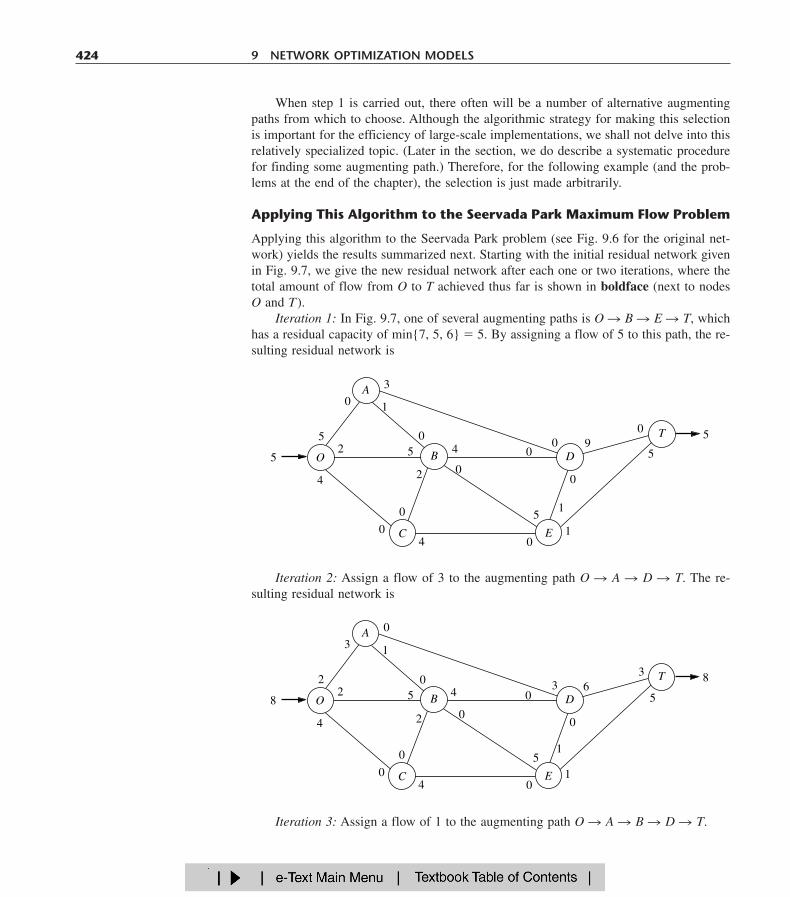
Applying this algorithm to the Seervada Park problem (see Fig. 9.6 for the original net-work) yields the results summarized next. Starting with the initial residual network givenin Fig. 9.7, we give the new residual network after each one or two iterations, where thetotal amount of flow from O to T achieved thus far is shown in boldface (next to nodesO and T).
Iteration 1: In Fig. 9.7, one of several augmenting paths is O � B � E � T, whichhas a residual capacity of min{7, 5, 6} � 5. By assigning a flow of 5 to this path, the re-sulting residual network is
424 9 NETWORK OPTIMIZATION MODELS
Iteration 2: Assign a flow of 3 to the augmenting path O � A � D � T. The re-sulting residual network is
5
1
0
4
2
51
4
2 55
5
0
3
1
05
4
0
0
E0
DB0
C
00 9
0 T
A
O
5
1
0
4
2
51
4
2 58
8
3
0
1
02
4
0
0
E0
DB0
C
03 6
3 T
A
O
Iteration 3: Assign a flow of 1 to the augmenting path O � A � B � D � T.
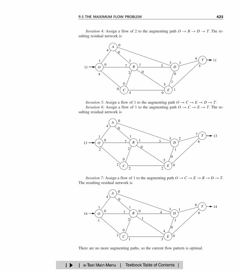
Iteration 4: Assign a flow of 2 to the augmenting path O � B � D � T. The re-sulting residual network is
9.5 THE MAXIMUM FLOW PROBLEM 425
Iteration 5: Assign a flow of 1 to the augmenting path O � C � E � D � T.Iteration 6: Assign a flow of 1 to the augmenting path O � C � E � T. The re-
sulting residual network is
Iteration 7: Assign a flow of 1 to the augmenting path O � C � E � B � D � T.The resulting residual network is
5
1
0
1
2
5
14
0 711
11
4
0
0
11
4
0
0
E0
DB
0
C
33 3
6 T
A
O
6
0
1
1
2
50
2
0 713
13
4
0
0
11
2
2
0
E2
DB0
C
33 2
7 T
A
O
6
0
1
0
2
40
1
0 714
14
4
0
0
11
1
3
0
E3
DB
1
C
43 1
8 T
A
O
There are no more augmenting paths, so the current flow pattern is optimal.

The current flow pattern may be identified by either cumulating the flow assignmentsor comparing the final residual capacities with the original arc capacities. If we use thelatter method, there is flow along an arc if the final residual capacity is less than the orig-inal capacity. The magnitude of this flow equals the difference in these capacities. Ap-plying this method by comparing the residual network obtained from the last iterationwith either Fig. 9.6 or 9.7 yields the optimal flow pattern shown in Fig. 9.8.
This example nicely illustrates the reason for replacing each directed arc i � j in theoriginal network by an undirected arc in the residual network and then increasing the resid-ual capacity for j � i by c* when a flow of c* is assigned to i � j. Without this refine-ment, the first six iterations would be unchanged. However, at that point it would appearthat no augmenting paths remain (because the real unused arc capacity for E � B is zero).Therefore, the refinement permits us to add the flow assignment of 1 for O � C � E �B � D � T in iteration 7. In effect, this additional flow assignment cancels 1 unit offlow assigned at iteration 1 (O � B � E � T) and replaces it by assignments of 1 unitof flow to both O � B � D � T and O � C � E � T.
Finding an Augmenting Path
The most difficult part of this algorithm when large networks are involved is finding anaugmenting path. This task may be simplified by the following systematic procedure. Be-gin by determining all nodes that can be reached from the source along a single arc withstrictly positive residual capacity. Then, for each of these nodes that were reached, deter-mine all new nodes (those not yet reached) that can be reached from this node along anarc with strictly positive residual capacity. Repeat this successively with the new nodesas they are reached. The result will be the identification of a tree of all the nodes that canbe reached from the source along a path with strictly positive residual flow capacity. Hence,this fanning-out procedure will always identify an augmenting path if one exists. The pro-cedure is illustrated in Fig. 9.9 for the residual network that results from iteration 6 in thepreceding example.
Although the procedure illustrated in Fig. 9.9 is a relatively straightforward one, itwould be helpful to be able to recognize when optimality has been reached without anexhaustive search for a nonexistent path. It is sometimes possible to recognize this eventbecause of an important theorem of network theory known as the max-flow min-cut the-orem. A cut may be defined as any set of directed arcs containing at least one arc from
426 9 NETWORK OPTIMIZATION MODELS
O
E
DB
A
8
1
3
4
4
7
1
3
3
4
6
14
14T
C
FIGURE 9.8Optimal solution for theSeervada Park maximum flowproblem.

every directed path from the source to the sink. There normally are many ways to slicethrough a network to form a cut to help analyze the network. For any particular cut, thecut value is the sum of the arc capacities of the arcs (in the specified direction) of thecut. The max-flow min-cut theorem states that, for any network with a single source andsink, the maximum feasible flow from the source to the sink equals the minimum cut valuefor all cuts of the network. Thus, if we let F denote the amount of flow from the sourceto the sink for any feasible flow pattern, the value of any cut provides an upper bound toF, and the smallest of the cut values is equal to the maximum value of F. Therefore, if acut whose value equals the value of F currently attained by the solution procedure can befound in the original network, the current flow pattern must be optimal. Eventually, opti-mality has been attained whenever there exists a cut in the residual network whose valueis zero.
To illustrate, consider the network of Fig. 9.7. One interesting cut through this net-work is shown in Fig. 9.10. Notice that the value of the cut is 3 � 4 � 1 � 6 � 14, whichwas found to be the maximum value of F, so this cut is a minimum cut. Notice also that,in the residual network resulting from iteration 7, where F � 14, the corresponding cuthas a value of zero. If this had been noticed, it would not have been necessary to searchfor additional augmenting paths.
9.5 THE MAXIMUM FLOW PROBLEM 427
O
E
D
T
B
A
7
62
05
2
0
0
1
2
1
0
0
04
22
10
2
7 33
1
C
FIGURE 9.9Procedure for finding anaugmenting path foriteration 7 of the SeervadaPark maximum flowproblem.
O
C
D
T00
0
57
4
0
0
0
2 5
40
0
0
1
6
0
09
0
4
3
1
A
B
E
FIGURE 9.10A minimum cut for theSeervada Park maximum flowproblem.
Using Excel to Formulate and Solve Maximum Flow Problems
Most maximum flow problems that arise in practice are considerably larger, and occa-sionally vastly larger, than the Seervada Park problem. Some problems have thousands ofnodes and arcs. The augmenting path algorithm just presented is far more efficient thanthe general simplex method for solving such large problems. However, for problems ofmodest size, a reasonable and convenient alternative is to use Excel and its Solver basedon the general simplex method.
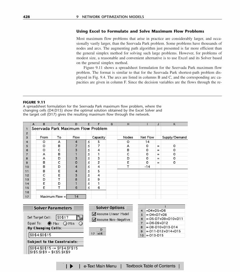
Figure 9.11 shows a spreadsheet formulation for the Seervada Park maximum flowproblem. The format is similar to that for the Seervada Park shortest-path problem dis-played in Fig. 9.4. The arcs are listed in columns B and C, and the corresponding arc ca-pacities are given in column F. Since the decision variables are the flows through the re-
428 9 NETWORK OPTIMIZATION MODELS
FIGURE 9.11A spreadsheet formulation for the Seervada Park maximum flow problem, where thechanging cells (D4:D15) show the optimal solution obtained by the Excel Solver andthe target cell (D17) gives the resulting maximum flow through the network.

spective arcs, these quantities are entered in the changing cells in column D (cells D4:D15).Employing the equations given in the bottom right-hand corner of the figure, these flowsthen are used to calculate the net flow generated at each of the nodes (see columns H andI). These net flows are required to be 0 for the transshipment nodes (A, B, C, D, and E),as indicated by the second set of constraints (I5:I9 � K5:K9) in the Solver dialogue box.The first set of constraints (D4:D15 � F4:F15) specifies the arc capacity constraints. Thetotal amount of flow from the source (node O) to the sink (node T) equals the flow gen-erated at the source (cell I4), so the target cell (D17) is set equal to I4. After specifyingmaximization of the target cell in the Solver dialogue box and then clicking on the Solvebutton, the optimal solution shown in cells D4:D15 is obtained.
9.6 THE MINIMUM COST FLOW PROBLEM 429
The minimum cost flow problem holds a central position among network optimization mod-els, both because it encompasses such a broad class of applications and because it can besolved extremely efficiently. Like the maximum flow problem, it considers flow through anetwork with limited arc capacities. Like the shortest-path problem, it considers a cost (ordistance) for flow through an arc. Like the transportation problem or assignment problem ofChap. 8, it can consider multiple sources (supply nodes) and multiple destinations (demandnodes) for the flow, again with associated costs. In fact, all four of these previously studiedproblems are special cases of the minimum cost flow problem, as we will demonstrate shortly.
The reason that the minimum cost flow problem can be solved so efficiently is thatit can be formulated as a linear programming problem so it can be solved by a stream-lined version of the simplex method called the network simplex method. We describe thisalgorithm in the next section.
The minimum cost flow problem is described below.
1. The network is a directed and connected network.2. At least one of the nodes is a supply node.3. At least one of the other nodes is a demand node.4. All the remaining nodes are transshipment nodes.5. Flow through an arc is allowed only in the direction indicated by the arrowhead, where
the maximum amount of flow is given by the capacity of that arc. (If flow can occur inboth directions, this would be represented by a pair of arcs pointing in opposite directions.)
6. The network has enough arcs with sufficient capacity to enable all the flow generatedat the supply nodes to reach all the demand nodes.
7. The cost of the flow through each arc is proportional to the amount of that flow, wherethe cost per unit flow is known.
8. The objective is to minimize the total cost of sending the available supply through thenetwork to satisfy the given demand. (An alternative objective is to maximize the to-tal profit from doing this.)
Some Applications
Probably the most important kind of application of minimum cost flow problems is to theoperation of a company’s distribution network. As summarized in the first row of Table9.3, this kind of application always involves determining a plan for shipping goods from
9.6 THE MINIMUM COST FLOW PROBLEM
its sources (factories, etc.) to intermediate storage facilities (as needed) and then on tothe customers.
For example, consider the distribution network for the International Paper Company(as described in the March–April 1988 issue of Interfaces). This company is the world’slargest manufacturer of pulp, paper, and paper products, as well as a major producer oflumber and plywood. It also either owns or has rights over about 20 million acres of wood-lands. The supply nodes in its distribution network are these woodlands in their variouslocations. However, before the company’s goods can eventually reach the demand nodes(the customers), the wood must pass through a long sequence of transshipment nodes. Atypical path through the distribution network is
Woodlands � woodyards � sawmills� paper mills � converting plants� warehouses � customers.
Another example of a complicated distribution network is the one for the Citgo Pe-troleum Corporation described in Sec. 3.5. Applying a minimum cost flow problem for-mulation to improve the operation of this distribution network saved Citgo at least $16.5million annually.
For some applications of minimum cost flow problems, all the transshipment nodesare processing facilities rather than intermediate storage facilities. This is the case forsolid waste management, as indicated in the second row of Table 9.3. Here, the flow ofmaterials through the network begins at the sources of the solid waste, then goes to thefacilities for processing these waste materials into a form suitable for landfill, and thensends them on to the various landfill locations. However, the objective still is to deter-mine the flow plan that minimizes the total cost, where the cost now is for both ship-ping and processing.
In other applications, the demand nodes might be processing facilities. For example,in the third row of Table 9.3, the objective is to find the minimum cost plan for obtain-ing supplies from various possible vendors, storing these goods in warehouses (as needed),and then shipping the supplies to the company’s processing facilities (factories, etc.). Sincethe total amount that could be supplied by all the vendors is more than the company needs,
430 9 NETWORK OPTIMIZATION MODELS
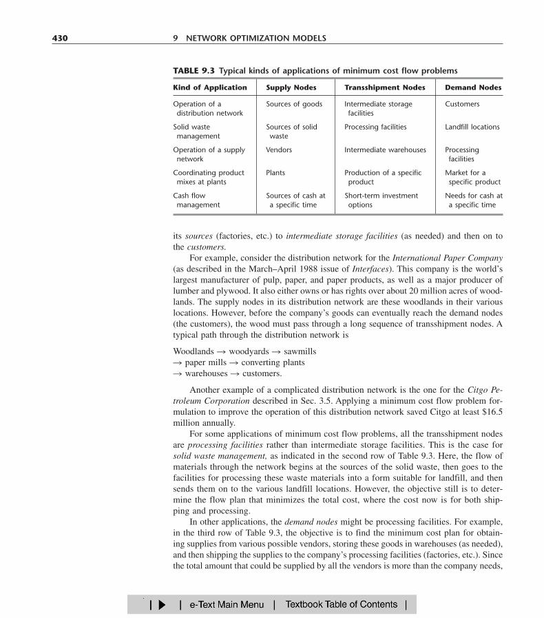
TABLE 9.3 Typical kinds of applications of minimum cost flow problems
Kind of Application Supply Nodes Transshipment Nodes Demand Nodes
Operation of a Sources of goods Intermediate storage Customersdistribution network facilities
Solid waste Sources of solid Processing facilities Landfill locationsmanagement waste
Operation of a supply Vendors Intermediate warehouses Processingnetwork facilities
Coordinating product Plants Production of a specific Market for amixes at plants product specific product
Cash flow Sources of cash at Short-term investment Needs for cash atmanagement a specific time options a specific time
the network includes a dummy demand node that receives (at zero cost) all the unusedsupply capacity at the vendors.
The July–August 1987 issue of Interfaces describes how, even back then, microcom-puters were being used by Marshalls, Inc. (an off-price retail chain) to deal with a mini-mum cost flow problem this way. In this application, Marshalls was optimizing the flowof freight from vendors to processing centers and then on to retail stores. Some of theirnetworks had over 20,000 arcs.
The next kind of application in Table 9.3 (coordinating product mixes at plants) illus-trates that arcs can represent something other than a shipping lane for a physical flow ofmaterials. This application involves a company with several plants (the supply nodes) thatcan produce the same products but at different costs. Each arc from a supply node repre-sents the production of one of the possible products at that plant, where this arc leads tothe transshipment node that corresponds to this product. Thus, this transshipment node hasan arc coming in from each plant capable of producing this product, and then the arcs lead-ing out of this node go to the respective customers (the demand nodes) for this product.The objective is to determine how to divide each plant’s production capacity among theproducts so as to minimize the total cost of meeting the demand for the various products.
The last application in Table 9.3 (cash flow management) illustrates that different nodescan represent some event that occurs at different times. In this case, each supply node rep-resents a specific time (or time period) when some cash will become available to the com-pany (through maturing accounts, notes receivable, sales of securities, borrowing, etc.). Thesupply at each of these nodes is the amount of cash that will become available then. Sim-ilarly, each demand node represents a specific time (or time period) when the company willneed to draw on its cash reserves. The demand at each such node is the amount of cashthat will be needed then. The objective is to maximize the company’s income from in-vesting the cash between each time it becomes available and when it will be used. There-fore, each transshipment node represents the choice of a specific short-term investment op-tion (e.g., purchasing a certificate of deposit from a bank) over a specific time interval. Theresulting network will have a succession of flows representing a schedule for cash becomingavailable, being invested, and then being used after the maturing of the investment.
Formulation of the Model
Consider a directed and connected network where the n nodes include at least one sup-ply node and at least one demand node. The decision variables are
xij � flow through arc i � j,
and the given information includes
cij � cost per unit flow through arc i � j,uij � arc capacity for arc i � j,bi � net flow generated at node i.
The value of bi depends on the nature of node i, where
bi � 0 if node i is a supply node,bi � 0 if node i is a demand node,bi � 0 if node i is a transshipment node.
9.6 THE MINIMUM COST FLOW PROBLEM 431

The objective is to minimize the total cost of sending the available supply through thenetwork to satisfy the given demand.
By using the convention that summations are taken only over existing arcs, the lin-ear programming formulation of this problem is
Minimize Z � �n
i�1�n
j�1cijxij,
subject to
�n
j�1xij � �
n
j�1xji � bi, for each node i,
and
0 � xij � uij, for each arc i � j.
The first summation in the node constraints represents the total flow out of node i, whereasthe second summation represents the total flow into node i, so the difference is the netflow generated at this node.
In some applications, it is necessary to have a lower bound Lij � 0 for the flow througheach arc i � j. When this occurs, use a translation of variables x�ij � xij � Lij, with x�ij �Lij substituted for xij throughout the model, to convert the model back to the above for-mat with nonnegativity constraints.
It is not guaranteed that the problem actually will possess feasible solutions, dependingpartially upon which arcs are present in the network and their arc capacities. However,for a reasonably designed network, the main condition needed is the following.
Feasible solutions property: A necessary condition for a minimum cost flowproblem to have any feasible solutions is that
�n
i�1bi � 0.
That is, the total flow being generated at the supply nodes equals the total flowbeing absorbed at the demand nodes.
If the values of bi provided for some application violate this condition, the usual interpreta-tion is that either the supplies or the demands (whichever are in excess) actually represent up-per bounds rather than exact amounts. When this situation arose for the transportation prob-lem in Sec. 8.1, either a dummy destination was added to receive the excess supply or adummy source was added to send the excess demand. The analogous step now is that eithera dummy demand node should be added to absorb the excess supply (with cij � 0 arcs addedfrom every supply node to this node) or a dummy supply node should be added to generatethe flow for the excess demand (with cij � 0 arcs added from this node to every demand node).
For many applications, bi and uij will have integer values, and implementation willrequire that the flow quantities xij also be integer. Fortunately, just as for the transporta-tion problem, this outcome is guaranteed without explicitly imposing integer constraintson the variables because of the following property.
432 9 NETWORK OPTIMIZATION MODELS
Integer solutions property: For minimum cost flow problems where every bi
and uij have integer values, all the basic variables in every basic feasible (BF)solution (including an optimal one) also have integer values.
An Example
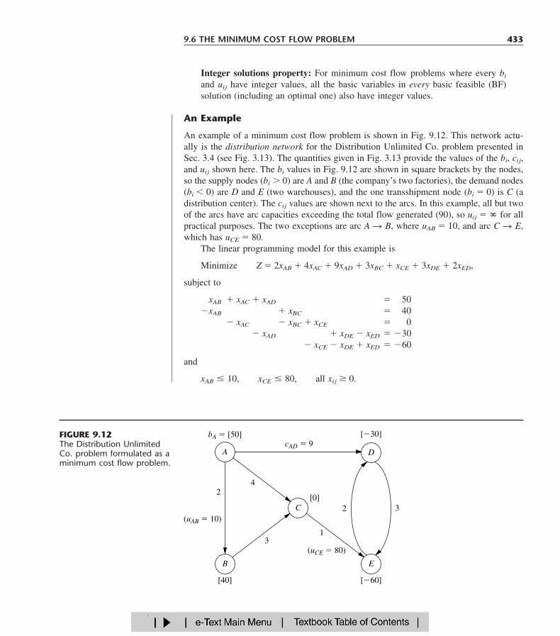
An example of a minimum cost flow problem is shown in Fig. 9.12. This network actu-ally is the distribution network for the Distribution Unlimited Co. problem presented inSec. 3.4 (see Fig. 3.13). The quantities given in Fig. 3.13 provide the values of the bi, cij,and uij shown here. The bi values in Fig. 9.12 are shown in square brackets by the nodes,so the supply nodes (bi � 0) are A and B (the company’s two factories), the demand nodes(bi � 0) are D and E (two warehouses), and the one transshipment node (bi � 0) is C (adistribution center). The cij values are shown next to the arcs. In this example, all but twoof the arcs have arc capacities exceeding the total flow generated (90), so uij � � for allpractical purposes. The two exceptions are arc A � B, where uAB � 10, and arc C � E,which has uCE � 80.
The linear programming model for this example is
Minimize Z � 2xAB � 4xAC � 9xAD � 3xBC � xCE � 3xDE � 2xED,
subject to
xAB � xAC � xAD � 50�xAB � xBC � 40
� xAC � xBC � xCE � 0� xAD � xDE � xED � �30
� xCE � xDE � xED � �60
and
xAB � 10, xCE � 80, all xij 0.
9.6 THE MINIMUM COST FLOW PROBLEM 433
(uAB � 10)
(uCE � 80)
bA � [50] [�30]
[40]
D
[�60]
[0]
A
3
E
24
cAD � 9
B
2
31
C
FIGURE 9.12The Distribution UnlimitedCo. problem formulated as aminimum cost flow problem.
Now note the pattern of coefficients for each variable in the set of five node constraints(the equality constraints). Each variable has exactly two nonzero coefficients, where oneis �1 and the other is �1. This pattern recurs in every minimum cost flow problem, andit is this special structure that leads to the integer solutions property.
Another implication of this special structure is that (any) one of the node constraintsis redundant. The reason is that summing all these constraint equations yields nothing butzeros on both sides (assuming feasible solutions exist, so the bi values sum to zero), sothe negative of any one of these equations equals the sum of the rest of the equations.With just n � 1 nonredundant node constraints, these equations provide just n � 1 basicvariables for a BF solution. In the next section, you will see that the network simplexmethod treats the xij � uij constraints as mirror images of the nonnegativity constraints,so the total number of basic variables is n � 1. This leads to a direct correspondence be-tween the n � 1 arcs of a spanning tree and the n � 1 basic variables—but more aboutthat story later.
Using Excel to Formulate and Solve Minimum Cost Flow Problems
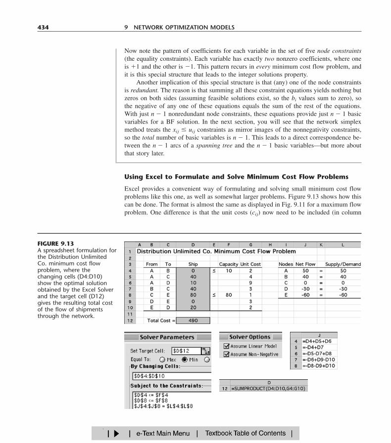
Excel provides a convenient way of formulating and solving small minimum cost flowproblems like this one, as well as somewhat larger problems. Figure 9.13 shows how thiscan be done. The format is almost the same as displayed in Fig. 9.11 for a maximum flowproblem. One difference is that the unit costs (cij) now need to be included (in column
434 9 NETWORK OPTIMIZATION MODELS
FIGURE 9.13A spreadsheet formulation forthe Distribution UnlimitedCo. minimum cost flowproblem, where thechanging cells (D4:D10)show the optimal solutionobtained by the Excel Solverand the target cell (D12)gives the resulting total costof the flow of shipmentsthrough the network.
G). Because bi values are specified for every node, net flow constraints are needed for allthe nodes. However, only two of the arcs happen to need arc capacity constraints. The tar-get cell (D12) now gives the total cost of the flow (shipments) through the network (seeits equation at the bottom of the figure), so the objective specified in the Solver dialoguebox is to minimize this quantity. The changing cells (D4:D10) in this spreadsheet showthe optimal solution obtained after clicking on the Solve button.
For much larger minimum cost flow problems, the network simplex method describedin the next section provides a considerably more efficient solution procedure. It also is anattractive option for solving various special cases of the minimum cost flow problem out-lined below. This algorithm is commonly included in mathematical programming soft-ware packages. For example, it is one of the options with CPLEX.
We shall soon solve this same example by the network simplex method. However, letus first see how some special cases fit into the network format of the minimum cost flowproblem.
Special Cases
The Transportation Problem. To formulate the transportation problem presented inSec. 8.1 as a minimum cost flow problem, a supply node is provided for each source, aswell as a demand node for each destination, but no transshipment nodes are included in thenetwork. All the arcs are directed from a supply node to a demand node, where distributingxij units from source i to destination j corresponds to a flow of xij through arc i � j. Thecost cij per unit distributed becomes the cost cij per unit of flow. Since the transportationproblem does not impose upper bound constraints on individual xij, all the uij � �.
Using this formulation for the P & T Co. transportation problem presented in Table8.2 yields the network shown in Fig. 8.2. The corresponding network for the general trans-portation problem is shown in Fig. 8.3.
The Assignment Problem. Since the assignment problem discussed in Sec. 8.3 is aspecial type of transportation problem, its formulation as a minimum cost flow problemfits into the same format. The additional factors are that (1) the number of supply nodesequals the number of demand nodes, (2) bi � 1 for each supply node, and (3) bi � �1for each demand node.
Figure 8.5 shows this formulation for the general assignment problem.
The Transshipment Problem. This special case actually includes all the general fea-tures of the minimum cost flow problem except for not having (finite) arc capacities. Thus,any minimum cost flow problem where each arc can carry any desired amount of flow isalso called a transshipment problem.
For example, the Distribution Unlimited Co. problem shown in Fig. 9.13 would be atransshipment problem if the upper bounds on the flow through arcs A � B and C � Ewere removed.
Transshipment problems frequently arise as generalizations of transportation prob-lems where units being distributed from each source to each destination can first passthrough intermediate points. These intermediate points may include other sources and des-tinations, as well as additional transfer points that would be represented by transshipmentnodes in the network representation of the problem. For example, the Distribution Un-
9.6 THE MINIMUM COST FLOW PROBLEM 435
limited Co. problem can be viewed as a generalization of a transportation problem withtwo sources (the two factories represented by nodes A and B in Fig. 9.13), two destina-tions (the two warehouses represented by nodes D and E), and one additional intermedi-ate transfer point (the distribution center represented by node C ).
(Chapter 23 on our website includes a further discussion of the transshipment problem.)
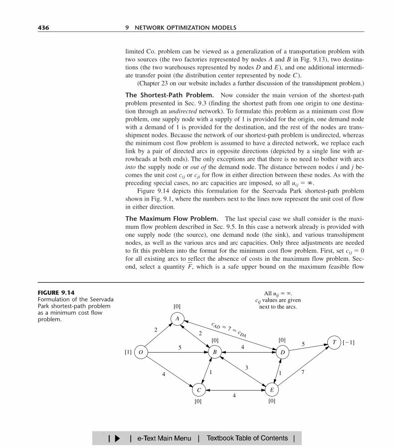
The Shortest-Path Problem. Now consider the main version of the shortest-pathproblem presented in Sec. 9.3 (finding the shortest path from one origin to one destina-tion through an undirected network). To formulate this problem as a minimum cost flowproblem, one supply node with a supply of 1 is provided for the origin, one demand nodewith a demand of 1 is provided for the destination, and the rest of the nodes are trans-shipment nodes. Because the network of our shortest-path problem is undirected, whereasthe minimum cost flow problem is assumed to have a directed network, we replace eachlink by a pair of directed arcs in opposite directions (depicted by a single line with ar-rowheads at both ends). The only exceptions are that there is no need to bother with arcsinto the supply node or out of the demand node. The distance between nodes i and j be-comes the unit cost cij or cji for flow in either direction between these nodes. As with thepreceding special cases, no arc capacities are imposed, so all uij � �.
Figure 9.14 depicts this formulation for the Seervada Park shortest-path problemshown in Fig. 9.1, where the numbers next to the lines now represent the unit cost of flowin either direction.
The Maximum Flow Problem. The last special case we shall consider is the maxi-mum flow problem described in Sec. 9.5. In this case a network already is provided withone supply node (the source), one demand node (the sink), and various transshipmentnodes, as well as the various arcs and arc capacities. Only three adjustments are neededto fit this problem into the format for the minimum cost flow problem. First, set cij � 0for all existing arcs to reflect the absence of costs in the maximum flow problem. Sec-ond, select a quantity F�, which is a safe upper bound on the maximum feasible flow
436 9 NETWORK OPTIMIZATION MODELS
O
E
DB
A
713
4
22
5
1
4
5
4
[1]
[�1]
[0]
[0]
[0][0]
[0] T
All uij � .cij values are given
next to the arcs.
cAD � 7 � cDA
C
FIGURE 9.14Formulation of the SeervadaPark shortest-path problemas a minimum cost flowproblem.
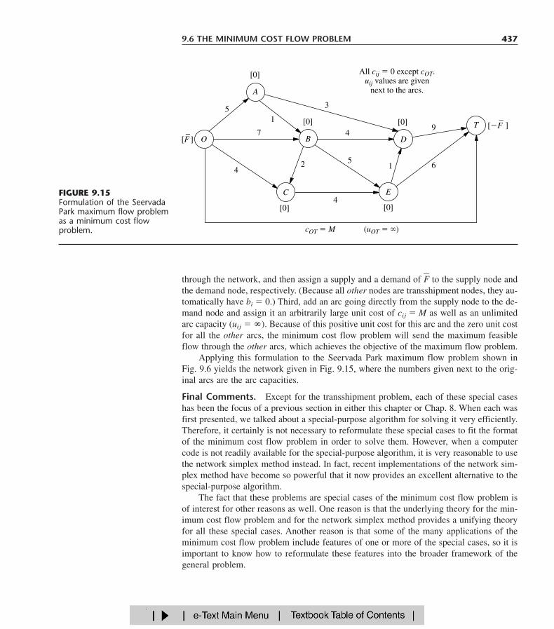
through the network, and then assign a supply and a demand of F� to the supply node andthe demand node, respectively. (Because all other nodes are transshipment nodes, they au-tomatically have bi � 0.) Third, add an arc going directly from the supply node to the de-mand node and assign it an arbitrarily large unit cost of cij � M as well as an unlimitedarc capacity (uij � �). Because of this positive unit cost for this arc and the zero unit costfor all the other arcs, the minimum cost flow problem will send the maximum feasibleflow through the other arcs, which achieves the objective of the maximum flow problem.
Applying this formulation to the Seervada Park maximum flow problem shown inFig. 9.6 yields the network given in Fig. 9.15, where the numbers given next to the orig-inal arcs are the arc capacities.
Final Comments. Except for the transshipment problem, each of these special caseshas been the focus of a previous section in either this chapter or Chap. 8. When each wasfirst presented, we talked about a special-purpose algorithm for solving it very efficiently.Therefore, it certainly is not necessary to reformulate these special cases to fit the formatof the minimum cost flow problem in order to solve them. However, when a computercode is not readily available for the special-purpose algorithm, it is very reasonable to usethe network simplex method instead. In fact, recent implementations of the network sim-plex method have become so powerful that it now provides an excellent alternative to thespecial-purpose algorithm.
The fact that these problems are special cases of the minimum cost flow problem isof interest for other reasons as well. One reason is that the underlying theory for the min-imum cost flow problem and for the network simplex method provides a unifying theoryfor all these special cases. Another reason is that some of the many applications of theminimum cost flow problem include features of one or more of the special cases, so it isimportant to know how to reformulate these features into the broader framework of thegeneral problem.
9.6 THE MINIMUM COST FLOW PROBLEM 437
O
E
B
615
3
4
51
9
2
4
7
4
[0]
[0]
[0][0]
All cij � 0 except cOT.uij values are given
next to the arcs.
C
[F�]
[�F�
cOT � M (uOT � )
]T
D
A
[0]
FIGURE 9.15Formulation of the SeervadaPark maximum flow problemas a minimum cost flowproblem.

438 9 NETWORK OPTIMIZATION MODELS
The network simplex method is a highly streamlined version of the simplex method forsolving minimum cost flow problems. As such, it goes through the same basic steps ateach iteration—finding the entering basic variable, determining the leaving basic variable,and solving for the new BF solution—in order to move from the current BF solution to abetter adjacent one. However, it executes these steps in ways that exploit the special net-work structure of the problem without ever needing a simplex tableau.
You may note some similarities between the network simplex method and the trans-portation simplex method presented in Sec. 8.2. In fact, both are streamlined versions ofthe simplex method that provide alternative algorithms for solving transportation prob-lems in similar ways. The network simplex method extends these ideas to solving othertypes of minimum cost flow problems as well.
In this section, we provide a somewhat abbreviated description of the network sim-plex method that focuses just on the main concepts. We omit certain details needed for afull computer implementation, including how to construct an initial BF solution and howto perform certain calculations (such as for finding the entering basic variable) in the mostefficient manner. These details are provided in various more specialized textbooks, suchas Selected References 1, 2, 3, 5, and 8.
Incorporating the Upper Bound Technique
The first concept is to incorporate the upper bound technique described in Sec. 7.3 to dealefficiently with the arc capacity constraints xij � uij. Thus, rather than these constraintsbeing treated as functional constraints, they are handled just as nonnegativity constraintsare. Therefore, they are considered only when the leaving basic variable is determined. Inparticular, as the entering basic variable is increased from zero, the leaving basic variableis the first basic variable that reaches either its lower bound (0) or its upper bound (uij).A nonbasic variable at its upper bound xij � uij is replaced by xij � uij � yij, so yij � 0becomes the nonbasic variable. See Sec. 7.3 for further details.
In our current context, yij has an interesting network interpretation. Whenever yij be-comes a basic variable with a strictly positive value (� uij), this value can be thought ofas flow from node j to node i (so in the “wrong” direction through arc i � j) that, in ac-tuality, is canceling that amount of the previously assigned flow (xij � uij) from node i tonode j. Thus, when xij � uij is replaced by xij � uij � yij, we also replace the real arc i � j by the reverse arc j � i, where this new arc has arc capacity uij (the maximumamount of the xij � uij flow that can be canceled) and unit cost � cij (since each unit offlow canceled saves cij). To reflect the flow of xij � uij through the deleted arc, we shiftthis amount of net flow generated from node i to node j by decreasing bi by uij and in-creasing bj by uij. Later, if yij becomes the leaving basic variable by reaching its upperbound, then yij � uij is replaced by yij � uij � xij with xij � 0 as the new nonbasic vari-able, so the above process would be reversed (replace arc j � i by arc i � j, etc.) to theoriginal configuration.
To illustrate this process, consider the minimum cost flow problem shown in Fig.9.12. While the network simplex method is generating a sequence of BF solutions, sup-pose that xAB has become the leaving basic variable for some iteration by reaching its up-per bound of 10. Consequently, xAB � 10 is replaced by xAB � 10 � yAB, so yAB � 0
9.7 THE NETWORK SIMPLEX METHOD
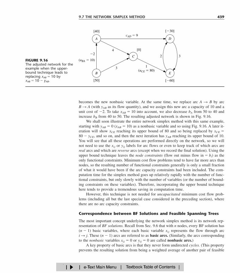
becomes the new nonbasic variable. At the same time, we replace arc A � B by arc B � A (with yAB as its flow quantity), and we assign this new arc a capacity of 10 and aunit cost of �2. To take xAB � 10 into account, we also decrease bA from 50 to 40 andincrease bB from 40 to 50. The resulting adjusted network is shown in Fig. 9.16.
We shall soon illustrate the entire network simplex method with this same example,starting with yAB � 0 (xAB � 10) as a nonbasic variable and so using Fig. 9.16. A later it-eration will show xCE reaching its upper bound of 80 and so being replaced by xCE �80 � yCE, and so on, and then the next iteration has yAB reaching its upper bound of 10.You will see that all these operations are performed directly on the network, so we willnot need to use the xij or yij labels for arc flows or even to keep track of which arcs arereal arcs and which are reverse arcs (except when we record the final solution). Using theupper bound technique leaves the node constraints (flow out minus flow in � bi) as theonly functional constraints. Minimum cost flow problems tend to have far more arcs thannodes, so the resulting number of functional constraints generally is only a small fractionof what it would have been if the arc capacity constraints had been included. The com-putation time for the simplex method goes up relatively rapidly with the number of func-tional constraints, but only slowly with the number of variables (or the number of bound-ing constraints on these variables). Therefore, incorporating the upper bound techniquehere tends to provide a tremendous saving in computation time.
However, this technique is not needed for uncapacitated minimum cost flow prob-lems (including all but the last special case considered in the preceding section), wherethere are no arc capacity constraints.
Correspondence between BF Solutions and Feasible Spanning Trees
The most important concept underlying the network simplex method is its network rep-resentation of BF solutions. Recall from Sec. 9.6 that with n nodes, every BF solution has(n � 1) basic variables, where each basic variable xij represents the flow through arc i � j. These (n � 1) arcs are referred to as basic arcs. (Similarly, the arcs correspondingto the nonbasic variables xij � 0 or yij � 0 are called nonbasic arcs.)
A key property of basic arcs is that they never form undirected cycles. (This propertyprevents the resulting solution from being a weighted average of another pair of feasible
9.7 THE NETWORK SIMPLEX METHOD 439
(uBA � 10)32
[�30]
[�60]
[40]
[50]
A
B
�24
3 1(uCE � 80)
cAD � 9
[0]
D
E
CFIGURE 9.16The adjusted network for theexample when the upper-bound technique leads toreplacing xAB � 10 by xAB � 10 � yAB.
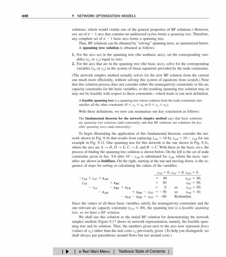
solutions, which would violate one of the general properties of BF solutions.) However,any set of n � 1 arcs that contains no undirected cycles forms a spanning tree. Therefore,any complete set of n � 1 basic arcs forms a spanning tree.
Thus, BF solutions can be obtained by “solving” spanning trees, as summarized below.A spanning tree solution is obtained as follows:
1. For the arcs not in the spanning tree (the nonbasic arcs), set the corresponding vari-ables (xij or yij) equal to zero.
2. For the arcs that are in the spanning tree (the basic arcs), solve for the correspondingvariables (xij or yij) in the system of linear equations provided by the node constraints.
(The network simplex method actually solves for the new BF solution from the currentone much more efficiently, without solving this system of equations from scratch.) Notethat this solution process does not consider either the nonnegativity constraints or the arccapacity constraints for the basic variables, so the resulting spanning tree solution may ormay not be feasible with respect to these constraints—which leads to our next definition.
A feasible spanning tree is a spanning tree whose solution from the node constraints alsosatisfies all the other constraints (0 � xij � uij or 0 � yij � uij).
With these definitions, we now can summarize our key conclusion as follows:
The fundamental theorem for the network simplex method says that basic solutionsare spanning tree solutions (and conversely) and that BF solutions are solutions for fea-sible spanning trees (and conversely).
To begin illustrating the application of this fundamental theorem, consider the net-work shown in Fig. 9.16 that results from replacing xAB � 10 by xAB � 10 � yAB for ourexample in Fig. 9.12. One spanning tree for this network is the one shown in Fig. 9.3e,where the arcs are A � D, D � E, C � E, and B � C. With these as the basic arcs, theprocess of finding the spanning tree solution is shown below. On the left is the set of nodeconstraints given in Sec. 9.6 after 10 � yAB is substituted for xAB, where the basic vari-ables are shown in boldface. On the right, starting at the top and moving down, is the se-quence of steps for setting or calculating the values of the variables.
yAB � 0, xAC � 0, xED � 0
�yAB � xAC � xAD � xBC � xCE � xDE � xED � �40 xAD � 40.�yAB � xAC � xAD � xBC � �50 xBC � 50.�yAB � xAC �xAD � xBC � xCE � � 0 so xCE � 50.�yAB � xAC� xAD � xBC � xCE � xDE � xED � �30 so xDE � 10.�yAB � xAC � xAD � xBC � xCE � xDE � xED � �60 Redundant.
Since the values of all these basic variables satisfy the nonnegativity constraints and theone relevant arc capacity constraint (xCE � 80), the spanning tree is a feasible spanningtree, so we have a BF solution.
We shall use this solution as the initial BF solution for demonstrating the networksimplex method. Figure 9.17 shows its network representation, namely, the feasible span-ning tree and its solution. Thus, the numbers given next to the arcs now represent flows(values of xij) rather than the unit costs cij previously given. (To help you distinguish, weshall always put parentheses around flows but not around costs.)
440 9 NETWORK OPTIMIZATION MODELS
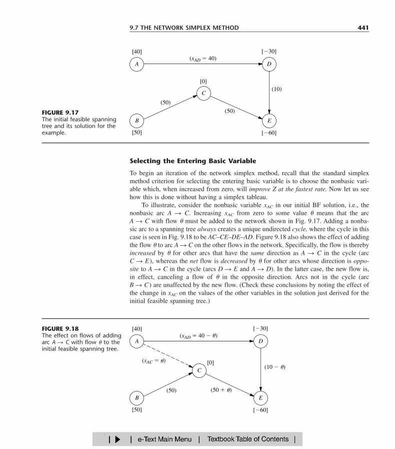
Selecting the Entering Basic Variable
To begin an iteration of the network simplex method, recall that the standard simplexmethod criterion for selecting the entering basic variable is to choose the nonbasic vari-able which, when increased from zero, will improve Z at the fastest rate. Now let us seehow this is done without having a simplex tableau.
To illustrate, consider the nonbasic variable xAC in our initial BF solution, i.e., thenonbasic arc A � C. Increasing xAC from zero to some value � means that the arc A � C with flow � must be added to the network shown in Fig. 9.17. Adding a nonba-sic arc to a spanning tree always creates a unique undirected cycle, where the cycle in thiscase is seen in Fig. 9.18 to be AC–CE–DE–AD. Figure 9.18 also shows the effect of addingthe flow � to arc A � C on the other flows in the network. Specifically, the flow is therebyincreased by � for other arcs that have the same direction as A � C in the cycle (arc C � E), whereas the net flow is decreased by � for other arcs whose direction is oppo-site to A � C in the cycle (arcs D � E and A � D). In the latter case, the new flow is,in effect, canceling a flow of � in the opposite direction. Arcs not in the cycle (arc B � C ) are unaffected by the new flow. (Check these conclusions by noting the effect ofthe change in xAC on the values of the other variables in the solution just derived for theinitial feasible spanning tree.)
9.7 THE NETWORK SIMPLEX METHOD 441
[�30]
[�60]
[40]
[50]
A
B
D
(50)
(50)
(10)[0]
(xAD � 40)
C
EFIGURE 9.17The initial feasible spanningtree and its solution for theexample.
[�30]
[�60]
[40]
[50]
A
B
D
(50) (50 � �)
(10 � �)[0]
(xAD � 40 � �)
C
E
(xAC � �)
�
�
�
�
FIGURE 9.18The effect on flows of addingarc A � C with flow � to theinitial feasible spanning tree.
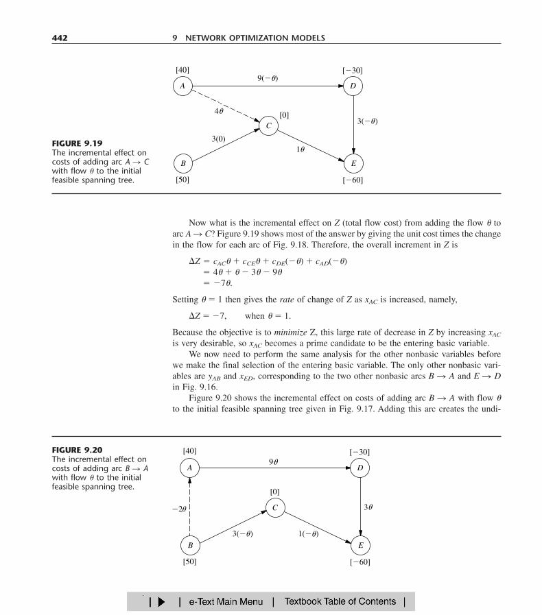
Now what is the incremental effect on Z (total flow cost) from adding the flow � toarc A � C? Figure 9.19 shows most of the answer by giving the unit cost times the changein the flow for each arc of Fig. 9.18. Therefore, the overall increment in Z is
�Z � cAC� � cCE� � cDE(��) � cAD(��)� 4� � � � 3� � 9�� �7�.
Setting � � 1 then gives the rate of change of Z as xAC is increased, namely,
�Z � �7, when � � 1.
Because the objective is to minimize Z, this large rate of decrease in Z by increasing xAC
is very desirable, so xAC becomes a prime candidate to be the entering basic variable.We now need to perform the same analysis for the other nonbasic variables before
we make the final selection of the entering basic variable. The only other nonbasic vari-ables are yAB and xED, corresponding to the two other nonbasic arcs B � A and E � Din Fig. 9.16.
Figure 9.20 shows the incremental effect on costs of adding arc B � A with flow �to the initial feasible spanning tree given in Fig. 9.17. Adding this arc creates the undi-
442 9 NETWORK OPTIMIZATION MODELS
[�30]
[�60]
[40]
[50]
A
B
D
3(0)
[0]
9(��)
C
E
4��
�
1��
3(��)�
FIGURE 9.19The incremental effect oncosts of adding arc A � Cwith flow � to the initialfeasible spanning tree.
[�30]
[�60]
[40]
[50]
A
B
D
[0]
3(��)
C
E
3� �2�
9��
�
� 1(��)�
�
FIGURE 9.20The incremental effect oncosts of adding arc B � Awith flow � to the initialfeasible spanning tree.
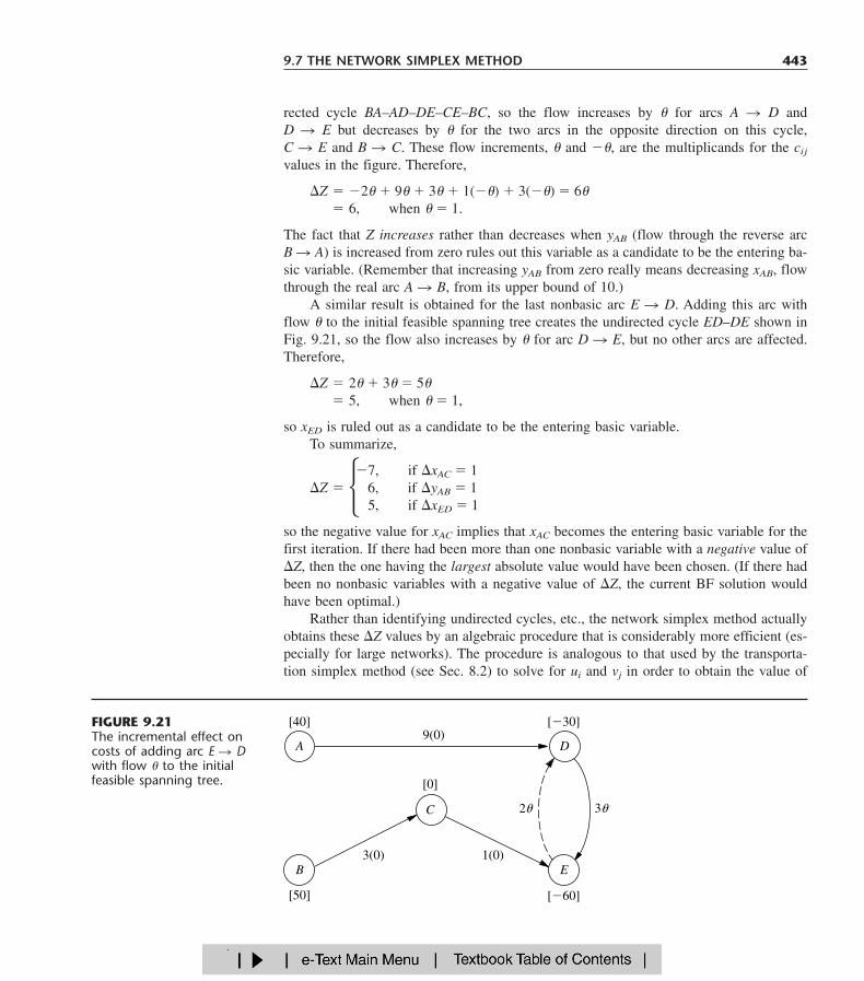
rected cycle BA–AD–DE–CE–BC, so the flow increases by � for arcs A � D and D � E but decreases by � for the two arcs in the opposite direction on this cycle,C � E and B � C. These flow increments, � and ��, are the multiplicands for the cij
values in the figure. Therefore,
�Z � �2� � 9� � 3� � 1(��) � 3(��) � 6�� 6, when � � 1.
The fact that Z increases rather than decreases when yAB (flow through the reverse arc B � A) is increased from zero rules out this variable as a candidate to be the entering ba-sic variable. (Remember that increasing yAB from zero really means decreasing xAB, flowthrough the real arc A � B, from its upper bound of 10.)
A similar result is obtained for the last nonbasic arc E � D. Adding this arc withflow � to the initial feasible spanning tree creates the undirected cycle ED–DE shown inFig. 9.21, so the flow also increases by � for arc D � E, but no other arcs are affected.Therefore,
�Z � 2� � 3� � 5�� 5, when � � 1,
so xED is ruled out as a candidate to be the entering basic variable.To summarize,
�7, if �xAC � 1�Z � � 6, if �yAB � 1
�5, if �xED � 1
so the negative value for xAC implies that xAC becomes the entering basic variable for thefirst iteration. If there had been more than one nonbasic variable with a negative value of�Z, then the one having the largest absolute value would have been chosen. (If there hadbeen no nonbasic variables with a negative value of �Z, the current BF solution wouldhave been optimal.)
Rather than identifying undirected cycles, etc., the network simplex method actuallyobtains these �Z values by an algebraic procedure that is considerably more efficient (es-pecially for large networks). The procedure is analogous to that used by the transporta-tion simplex method (see Sec. 8.2) to solve for ui and vj in order to obtain the value of
9.7 THE NETWORK SIMPLEX METHOD 443
3�
[�30]
[�60]
[40]
[50]
A
B3(0)
9(0)
1(0)
[0]
D
�2��
E
C
FIGURE 9.21The incremental effect oncosts of adding arc E � Dwith flow � to the initialfeasible spanning tree.
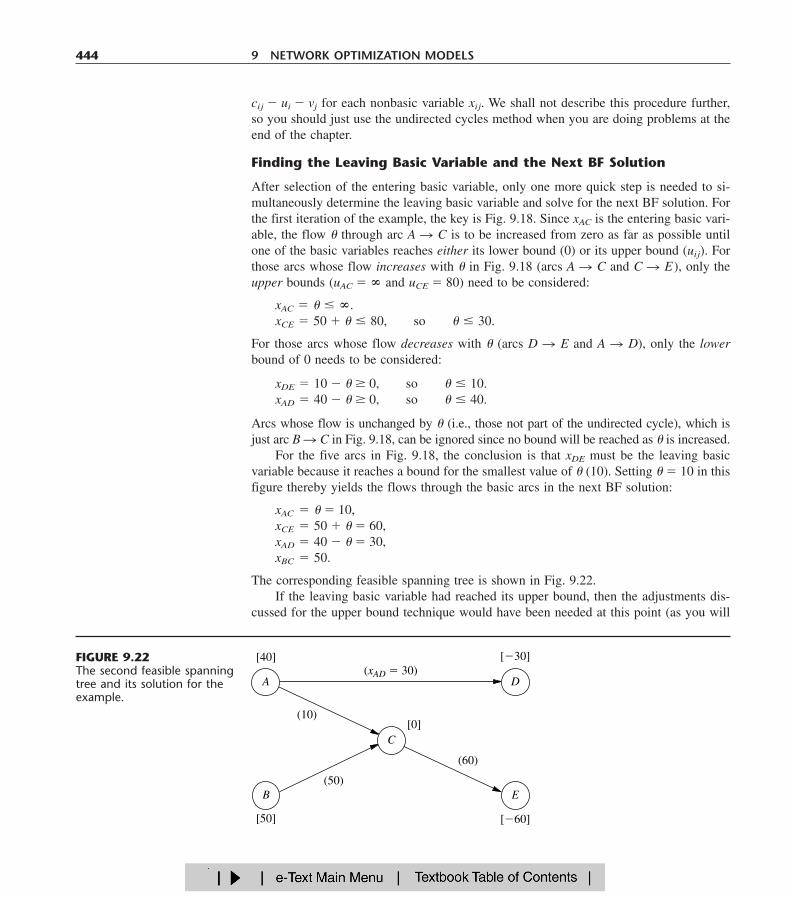
cij � ui � vj for each nonbasic variable xij. We shall not describe this procedure further,so you should just use the undirected cycles method when you are doing problems at theend of the chapter.
Finding the Leaving Basic Variable and the Next BF Solution
After selection of the entering basic variable, only one more quick step is needed to si-multaneously determine the leaving basic variable and solve for the next BF solution. Forthe first iteration of the example, the key is Fig. 9.18. Since xAC is the entering basic vari-able, the flow � through arc A � C is to be increased from zero as far as possible untilone of the basic variables reaches either its lower bound (0) or its upper bound (uij). Forthose arcs whose flow increases with � in Fig. 9.18 (arcs A � C and C � E), only theupper bounds (uAC � � and uCE � 80) need to be considered:
xAC � � � �.xCE � 50 � � � 80, so � � 30.
For those arcs whose flow decreases with � (arcs D � E and A � D), only the lowerbound of 0 needs to be considered:
xDE � 10 � � 0, so � � 10.xAD � 40 � � 0, so � � 40.
Arcs whose flow is unchanged by � (i.e., those not part of the undirected cycle), which isjust arc B � C in Fig. 9.18, can be ignored since no bound will be reached as � is increased.
For the five arcs in Fig. 9.18, the conclusion is that xDE must be the leaving basicvariable because it reaches a bound for the smallest value of � (10). Setting � � 10 in thisfigure thereby yields the flows through the basic arcs in the next BF solution:
xAC � � � 10,xCE � 50 � � � 60,xAD � 40 � � � 30,xBC � 50.
The corresponding feasible spanning tree is shown in Fig. 9.22.If the leaving basic variable had reached its upper bound, then the adjustments dis-
cussed for the upper bound technique would have been needed at this point (as you will
444 9 NETWORK OPTIMIZATION MODELS
[�30]
[�60]
[40]
[50]
A
B
D
[0]C
E
(xAD � 30)
(10)
(50)
(60)
FIGURE 9.22The second feasible spanningtree and its solution for theexample.
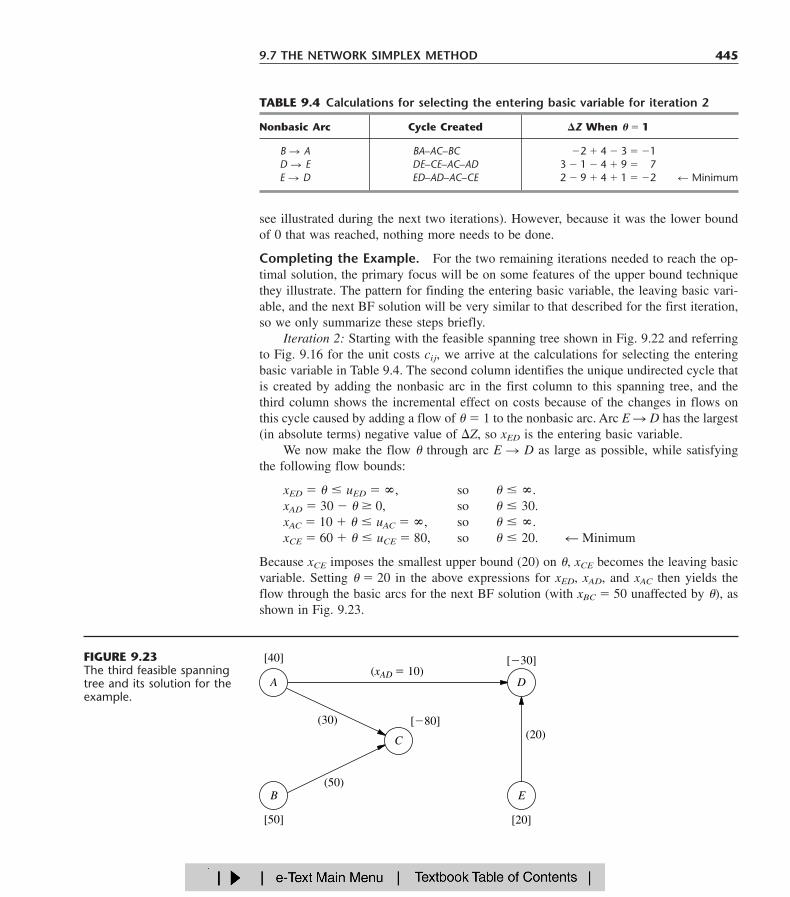
see illustrated during the next two iterations). However, because it was the lower boundof 0 that was reached, nothing more needs to be done.
Completing the Example. For the two remaining iterations needed to reach the op-timal solution, the primary focus will be on some features of the upper bound techniquethey illustrate. The pattern for finding the entering basic variable, the leaving basic vari-able, and the next BF solution will be very similar to that described for the first iteration,so we only summarize these steps briefly.
Iteration 2: Starting with the feasible spanning tree shown in Fig. 9.22 and referringto Fig. 9.16 for the unit costs cij, we arrive at the calculations for selecting the enteringbasic variable in Table 9.4. The second column identifies the unique undirected cycle thatis created by adding the nonbasic arc in the first column to this spanning tree, and thethird column shows the incremental effect on costs because of the changes in flows onthis cycle caused by adding a flow of � � 1 to the nonbasic arc. Arc E � D has the largest(in absolute terms) negative value of �Z, so xED is the entering basic variable.
We now make the flow � through arc E � D as large as possible, while satisfyingthe following flow bounds:
xED � � � uED � �, so � � �.xAD � 30 � � 0, so � � 30.xAC � 10 � � � uAC � �, so � � �.xCE � 60 � � � uCE � 80, so � � 20. � Minimum
Because xCE imposes the smallest upper bound (20) on �, xCE becomes the leaving basicvariable. Setting � � 20 in the above expressions for xED, xAD, and xAC then yields theflow through the basic arcs for the next BF solution (with xBC � 50 unaffected by �), asshown in Fig. 9.23.
9.7 THE NETWORK SIMPLEX METHOD 445
TABLE 9.4 Calculations for selecting the entering basic variable for iteration 2
Nonbasic Arc Cycle Created �Z When � � 1
B � A BA–AC–BC 2 �2 � 4 � 3 � �1D � E DE–CE–AC–AD 3 � 1 � 4 � 9 � �7E � D ED–AD–AC–CE 2 � 9 � 4 � 1 � �2 � Minimum
[�30]
[20]
[40]
[50]
A
B
D
(50)
(20)[�80]
(xAD � 10)
C
E
(30)
FIGURE 9.23The third feasible spanningtree and its solution for theexample.
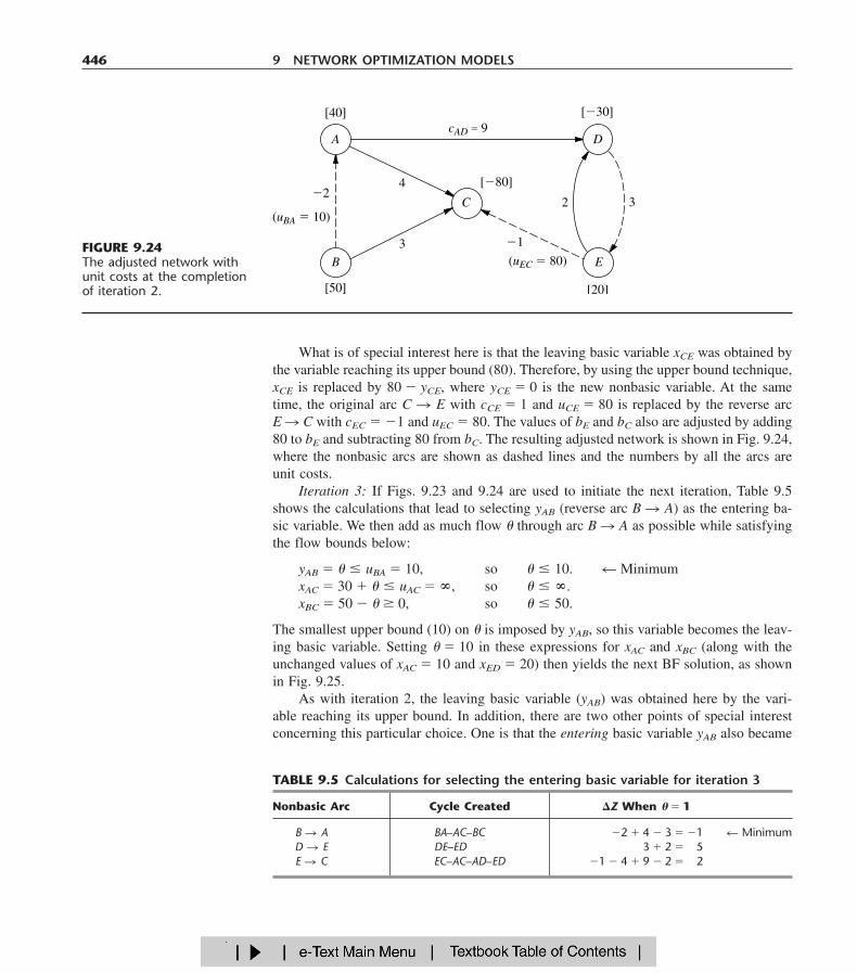
What is of special interest here is that the leaving basic variable xCE was obtained bythe variable reaching its upper bound (80). Therefore, by using the upper bound technique,xCE is replaced by 80 � yCE, where yCE � 0 is the new nonbasic variable. At the sametime, the original arc C � E with cCE � 1 and uCE � 80 is replaced by the reverse arc E � C with cEC � �1 and uEC � 80. The values of bE and bC also are adjusted by adding80 to bE and subtracting 80 from bC. The resulting adjusted network is shown in Fig. 9.24,where the nonbasic arcs are shown as dashed lines and the numbers by all the arcs areunit costs.
Iteration 3: If Figs. 9.23 and 9.24 are used to initiate the next iteration, Table 9.5shows the calculations that lead to selecting yAB (reverse arc B � A) as the entering ba-sic variable. We then add as much flow � through arc B � A as possible while satisfyingthe flow bounds below:
yAB � � � uBA � 10, so � � 10. � MinimumxAC � 30 � � � uAC � �, so � � �.xBC � 50 � � 0, so � � 50.
The smallest upper bound (10) on � is imposed by yAB, so this variable becomes the leav-ing basic variable. Setting � � 10 in these expressions for xAC and xBC (along with theunchanged values of xAC � 10 and xED � 20) then yields the next BF solution, as shownin Fig. 9.25.
As with iteration 2, the leaving basic variable (yAB) was obtained here by the vari-able reaching its upper bound. In addition, there are two other points of special interestconcerning this particular choice. One is that the entering basic variable yAB also became
446 9 NETWORK OPTIMIZATION MODELS
32
[�30]
[�80]
[20]
[40]
[50]
B E
3
4
cAD � 9
�1
C
A
�2
(uBA � 10)
(uEC � 80)
D
TABLE 9.5 Calculations for selecting the entering basic variable for iteration 3
Nonbasic Arc Cycle Created �Z When � � 1
B � A BA–AC–BC �1 �2 � 4 � 3 � �1 � MinimumD � E DE–ED �1 �2 � 3 � 2 � �5E � C EC–AC–AD–ED �1 � 4 � 9 � 2 � �2
FIGURE 9.24The adjusted network withunit costs at the completionof iteration 2.

the leaving basic variable on the same iteration! This event occurs occasionally with theupper bound technique whenever increasing the entering basic variable from zero causesits upper bound to be reached first before any of the other basic variables reach a bound.
The other interesting point is that the arc B � A that now needs to be replaced by areverse arc A � B (because of the leaving basic variable reaching an upper bound) al-ready is a reverse arc! This is no problem, because the reverse arc for a reverse arc is sim-ply the original real arc. Therefore, the arc B � A (with cBA � �2 and uBA � 10) in Fig.9.24 now is replaced by arc A � B (with cAB � 2 and uAB � 10), which is the arc be-tween nodes A and B in the original network shown in Fig. 9.12, and a generated net flowof 10 is shifted from node B (bB � 50 � 40) to node A (bA � 40 � 50). Simultaneously,the variable yAB � 10 is replaced by 10 � xAB, with xAB � 0 as the new nonbasic vari-able. The resulting adjusted network is shown in Fig. 9.26.
Passing the Optimality Test: At this point, the algorithm would attempt to use Figs.9.25 and 9.26 to find the next entering basic variable with the usual calculations shownin Table 9.6. However, none of the nonbasic arcs gives a negative value of �Z, so an im-provement in Z cannot be achieved by introducing flow through any of them. This meansthat the current BF solution shown in Fig. 9.25 has passed the optimality test, so the al-gorithm stops.
To identify the flows through real arcs rather than reverse arcs for this optimal solu-tion, the current adjusted network (Fig. 9.26) should be compared with the original net-work (Fig. 9.12). Note that each of the arcs has the same direction in the two networkswith the one exception of the arc between nodes C and E. This means that the only re-
9.7 THE NETWORK SIMPLEX METHOD 447
[�30]
[�80]
[20]
[50]
[40]
A
B
D
C
E
(xAD � 10)
(40)
(40)
(20)
TABLE 9.6 Calculations for the optimality test at the end of iteration 3
Nonbasic Arc Cycle Created �Z When � � 1
A � B AB–BC–AC 2 � 3 � 4 � 1D � E DE–EC–AC–AD 3 � 1 � 4 � 9 � 7E � C EC–AC–AD–ED �1 � 4 � 9 � 2 � 2
FIGURE 9.25The fourth (and final) feasiblespanning tree and itssolution for the example.
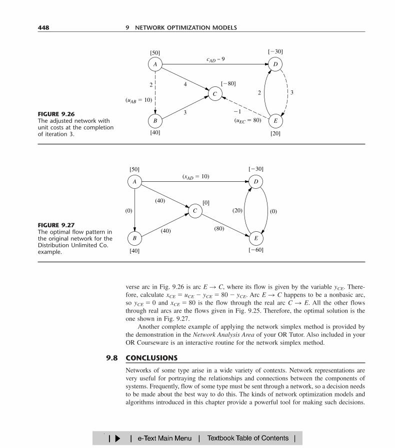
verse arc in Fig. 9.26 is arc E � C, where its flow is given by the variable yCE. There-fore, calculate xCE � uCE � yCE � 80 � yCE. Arc E � C happens to be a nonbasic arc,so yCE � 0 and xCE � 80 is the flow through the real arc C � E. All the other flowsthrough real arcs are the flows given in Fig. 9.25. Therefore, the optimal solution is theone shown in Fig. 9.27.
Another complete example of applying the network simplex method is provided bythe demonstration in the Network Analysis Area of your OR Tutor. Also included in yourOR Courseware is an interactive routine for the network simplex method.
448 9 NETWORK OPTIMIZATION MODELS
(0)(20)
[�30]
[0]
[�60]
[50]
[40]
B E(40)
(40)
(xAD � 10)
(80)
C
A
(0)
D
Networks of some type arise in a wide variety of contexts. Network representations arevery useful for portraying the relationships and connections between the components ofsystems. Frequently, flow of some type must be sent through a network, so a decision needsto be made about the best way to do this. The kinds of network optimization models andalgorithms introduced in this chapter provide a powerful tool for making such decisions.
9.8 CONCLUSIONS
FIGURE 9.27The optimal flow pattern inthe original network for theDistribution Unlimited Co.example.
32
[�30]
[�80]
[20]
[50]
[40]
B E3
4
cAD � 9
�1
C
A
2
(uAB � 10)
(uEC � 80)
D
FIGURE 9.26The adjusted network withunit costs at the completionof iteration 3.
The minimum cost flow problem plays a central role among these network opti-mization models, both because it is so broadly applicable and because it can be solvedextremely efficiently by the network simplex method. Two of its special cases includedin this chapter, the shortest-path problem and the maximum flow problem, also are basicnetwork optimization models, as are additional special cases discussed in Chap. 8 (thetransportation problem and the assignment problem).
Whereas all these models are concerned with optimizing the operation of an existingnetwork, the minimum spanning tree problem is a prominent example of a model for op-timizing the design of a new network.
This chapter has only scratched the surface of the current state of the art of networkmethodology. Because of their combinatorial nature, network problems often are extremelydifficult to solve. However, great progress is being made in developing powerful model-ing techniques and solution methodologies that are opening up new vistas for importantapplications. In fact, recent algorithmic advances are enabling us to solve successfullysome complex network problems of enormous size.
LEARNING AIDS FOR THIS CHAPTER IN YOUR OR COURSEWARE 449
1. Ahuja, R. K., T. L. Magnanti, and J. B. Orlin: Network Flows: Theory, Algorithms, and Appli-cations, Prentice-Hall, Englewood Cliffs, NJ, 1993.
2. Ball, M., T. L. Magnanti, C. Monma, and G. L. Nemhauser: Network Models, Elsevier, NewYork, 1995.
3. Bazaraa, M. S., J. J. Jarvis, and H. D. Sherali: Linear Programming and Network Flows, 2d ed.,Wiley, New York, 1990.
4. Dantzig, G. B., and M. N. Thapa: Linear Programming 1: Introduction, Springer, New York,1997, chap. 9.
5. Glover, F., D. Klingman, and N. V. Phillips: Network Models in Optimization and Their Appli-cations in Practice, Wiley, New York, 1992.
6. Hillier, F. S., M. S. Hillier, and G. J. Lieberman: Introduction to Management Science: A Mod-eling and Case Studies Approach with Spreadsheets, Irwin/McGraw-Hill, Burr Ridge, IL, 2000,chap. 7.
7. Magnanti, T. L., and R. T. Wong: “Network Design and Transportation Planning: Models andAlgorithms,” Transportation Science, 18: 1–55, 1984.
8. Murty, K. G.: Network Programming, Prentice-Hall, Englewood Cliffs, NJ, 1992.
SELECTED REFERENCES
A Demonstration Example in OR Tutor:
Network Simplex Method
An Interactive Routine:
Network Simplex Method—Interactive
LEARNING AIDS FOR THIS CHAPTER IN YOUR OR COURSEWARE

An Excel Add-in:
Premium Solver
“Ch. 9—Network Opt Models” Files for Solving the Examples:
Excel FileLINGO/LINDO FileMPL/CPLEX File
See Appendix 1 for documentation of the software.
450 9 NETWORK OPTIMIZATION MODELS
The symbols to the left of some of the problems (or their parts)have the following meaning:
D: The demonstration example listed above may be helpful.I: We suggest that you use the interactive routine listed above (the
printout records your work).C: Use the computer with any of the software options available to
you (or as instructed by your instructor) to solve the problem.
An asterisk on the problem number indicates that at least a partialanswer is given in the back of the book.
9.2-1. Consider the following directed network.
PROBLEMS
shows the mileage along each road that directly connects twotowns without any intervening towns. These numbers are sum-marized in the following table, where a dash indicates that thereis no road directly connecting these two towns without goingthrough any other towns.
Miles between Adjacent Towns
Town A B C D E Destination
Origin 40 60 50 — — —A 10 — 70 — —B 20 55 40 —C — 50 —D 10 60E 80
(a) Find a directed path from node A to node F, and then identifythree other undirected paths from node A to node F.
(b) Find three directed cycles. Then identify an undirected cyclethat includes every node.
(c) Identify a set of arcs that forms a spanning tree.(d) Use the process illustrated in Fig. 9.3 to grow a tree one arc
at a time until a spanning tree has been formed. Then repeatthis process to obtain another spanning tree. [Do not duplicatethe spanning tree identified in part (c).]
9.3-1. You need to take a trip by car to another town that youhave never visited before. Therefore, you are studying a map todetermine the shortest route to your destination. Depending onwhich route you choose, there are five other towns (call them A,B, C, D, E) that you might pass through on the way. The map
A
B
C
D
E
F(a) Formulate this problem as a shortest-path problem by drawing
a network where nodes represent towns, links represent roads,and numbers indicate the length of each link in miles.
(b) Use the algorithm described in Sec. 9.3 to solve this shortest-path problem.
C (c) Formulate and solve a spreadsheet model for this problem.(d) If each number in the table represented your cost (in dollars)
for driving your car from one town to the next, would the an-swer in part (b) or (c) now give your minimum cost route?
(e) If each number in the table represented your time (in minutes)for driving your car from one town to the next, would the an-swer in part (b) or (c) now give your minimum time route?
9.3-2. At a small but growing airport, the local airline company ispurchasing a new tractor for a tractor-trailer train to bring luggageto and from the airplanes. A new mechanized luggage system willbe installed in 3 years, so the tractor will not be needed after that.However, because it will receive heavy use, so that the running and
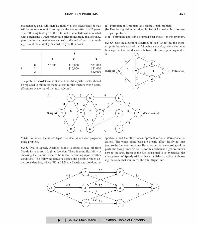
(Origin) (Destination)T
E
D
O B
C
A
4
6
52
5
7
5
4
6
8
1
(a)
1
maintenance costs will increase rapidly as the tractor ages, it maystill be more economical to replace the tractor after 1 or 2 years.The following table gives the total net discounted cost associatedwith purchasing a tractor (purchase price minus trade-in allowance,plus running and maintenance costs) at the end of year i and trad-ing it in at the end of year j (where year 0 is now).
CHAPTER 9 PROBLEMS 451
The problem is to determine at what times (if any) the tractor shouldbe replaced to minimize the total cost for the tractors over 3 years.(Continue at the top of the next column.)
j
1 2 3
0 $8,000 $18,000 $31,000i 1 $10,000 $21,000
2 $12,000
T(Origin) (Destination)O
B E I
A D G
HFC
4
3 4
2 225
6
34 5
2
1 2
5 8
43
72
6 5
(a)
(a) Formulate this problem as a shortest-path problem.(b) Use the algorithm described in Sec. 9.3 to solve this shortest-
path problem.C (c) Formulate and solve a spreadsheet model for this problem.
9.3-3.* Use the algorithm described in Sec. 9.3 to find the short-est path through each of the following networks, where the num-bers represent actual distances between the corresponding nodes.
9.3-4. Formulate the shortest-path problem as a linear program-ming problem.
9.3-5. One of Speedy Airlines’ flights is about to take off fromSeattle for a nonstop flight to London. There is some flexibility inchoosing the precise route to be taken, depending upon weatherconditions. The following network depicts the possible routes un-der consideration, where SE and LN are Seattle and London, re-
(b)
spectively, and the other nodes represent various intermediate lo-cations. The winds along each arc greatly affect the flying time(and so the fuel consumption). Based on current meteorological re-ports, the flying times (in hours) for this particular flight are shownnext to the arcs. Because the fuel consumed is so expensive, themanagement of Speedy Airlines has established a policy of choos-ing the route that minimizes the total flight time.
LNSE B E
C F
A D
4.2 3.8
4.7 3.6
4.6
3.5
3.4
3.6
3.3
3.5
3.2
3.4
3.4
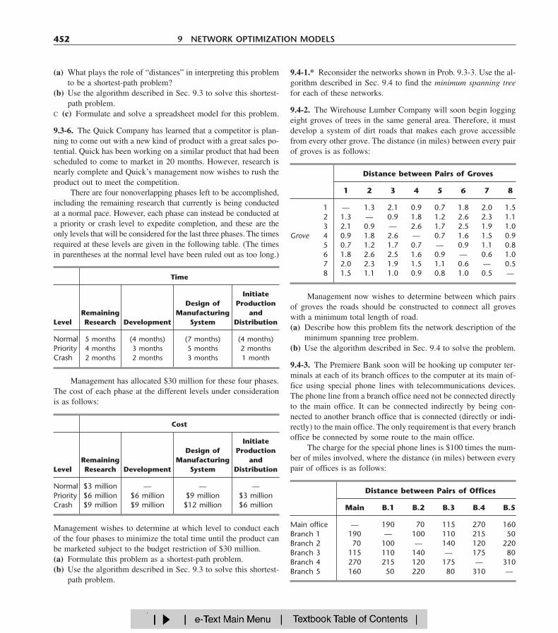
9.4-1.* Reconsider the networks shown in Prob. 9.3-3. Use the al-gorithm described in Sec. 9.4 to find the minimum spanning treefor each of these networks.
9.4-2. The Wirehouse Lumber Company will soon begin loggingeight groves of trees in the same general area. Therefore, it mustdevelop a system of dirt roads that makes each grove accessiblefrom every other grove. The distance (in miles) between every pairof groves is as follows:
(a) What plays the role of “distances” in interpreting this problemto be a shortest-path problem?
(b) Use the algorithm described in Sec. 9.3 to solve this shortest-path problem.
C (c) Formulate and solve a spreadsheet model for this problem.
9.3-6. The Quick Company has learned that a competitor is plan-ning to come out with a new kind of product with a great sales po-tential. Quick has been working on a similar product that had beenscheduled to come to market in 20 months. However, research isnearly complete and Quick’s management now wishes to rush theproduct out to meet the competition.
There are four nonoverlapping phases left to be accomplished,including the remaining research that currently is being conductedat a normal pace. However, each phase can instead be conducted ata priority or crash level to expedite completion, and these are theonly levels that will be considered for the last three phases. The timesrequired at these levels are given in the following table. (The timesin parentheses at the normal level have been ruled out as too long.)
452 9 NETWORK OPTIMIZATION MODELS
Management has allocated $30 million for these four phases.The cost of each phase at the different levels under considerationis as follows:
Cost
InitiateDesign of Production
Remaining Manufacturing andLevel Research Development System Distribution
Normal $3 million — — —Priority $6 million $6 million $9 million $3 millionCrash $9 million $9 million $12 million $6 million
Time
InitiateDesign of Production
Remaining Manufacturing andLevel Research Development System Distribution
Normal 5 months (4 months) (7 months) (4 months)Priority 4 months 3 months 5 months 2 monthsCrash 2 months 2 months 3 months 1 month
Management wishes to determine at which level to conduct eachof the four phases to minimize the total time until the product canbe marketed subject to the budget restriction of $30 million.(a) Formulate this problem as a shortest-path problem.(b) Use the algorithm described in Sec. 9.3 to solve this shortest-
path problem.
Distance between Pairs of Groves
1 2 3 4 5 6 7 8
1 — 1.3 2.1 0.9 0.7 1.8 2.0 1.52 1.3 — 0.9 1.8 1.2 2.6 2.3 1.13 2.1 0.9 — 2.6 1.7 2.5 1.9 1.0
Grove 4 0.9 1.8 2.6 — 0.7 1.6 1.5 0.95 0.7 1.2 1.7 0.7 — 0.9 1.1 0.86 1.8 2.6 2.5 1.6 0.9 — 0.6 1.07 2.0 2.3 1.9 1.5 1.1 0.6 — 0.58 1.5 1.1 1.0 0.9 0.8 1.0 0.5 —
Management now wishes to determine between which pairsof groves the roads should be constructed to connect all groveswith a minimum total length of road.(a) Describe how this problem fits the network description of the
minimum spanning tree problem.(b) Use the algorithm described in Sec. 9.4 to solve the problem.
9.4-3. The Premiere Bank soon will be hooking up computer ter-minals at each of its branch offices to the computer at its main of-fice using special phone lines with telecommunications devices.The phone line from a branch office need not be connected directlyto the main office. It can be connected indirectly by being con-nected to another branch office that is connected (directly or indi-rectly) to the main office. The only requirement is that every branchoffice be connected by some route to the main office.
The charge for the special phone lines is $100 times the num-ber of miles involved, where the distance (in miles) between everypair of offices is as follows:
Distance between Pairs of Offices
Main B.1 B.2 B.3 B.4 B.5
Main office — 190 70 115 270 160Branch 1 190 — 100 110 215 50Branch 2 70 100 — 140 120 220Branch 3 115 110 140 — 175 80Branch 4 270 215 120 175 — 310Branch 5 160 50 220 80 310 —
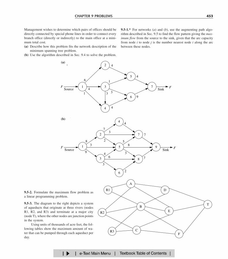
(b)
SourceF
SinkF
7
4
2
3 8
51 9
6
83
9
73
2
46
3
2
58
3
4
7
7
Source Sink7
6
5
3
4
4
6
1 3
4
4
1
4
9
(a)
3
F F
2
1
Management wishes to determine which pairs of offices should bedirectly connected by special phone lines in order to connect everybranch office (directly or indirectly) to the main office at a mini-mum total cost.(a) Describe how this problem fits the network description of the
minimum spanning tree problem.(b) Use the algorithm described in Sec. 9.4 to solve the problem.
CHAPTER 9 PROBLEMS 453
(b)
9.5-2. Formulate the maximum flow problem asa linear programming problem.
9.5-3. The diagram to the right depicts a systemof aqueducts that originate at three rivers (nodesR1, R2, and R3) and terminate at a major city(node T), where the other nodes are junction pointsin the system.
Using units of thousands of acre feet, the fol-lowing tables show the maximum amount of wa-ter that can be pumped through each aqueduct perday.
(a)
9.5-1.* For networks (a) and (b), use the augmenting path algo-rithm described in Sec. 9.5 to find the flow pattern giving the max-imum flow from the source to the sink, given that the arc capacityfrom node i to node j is the number nearest node i along the arcbetween these nodes.
A
CF
R3
R1 D
BE
T
R2
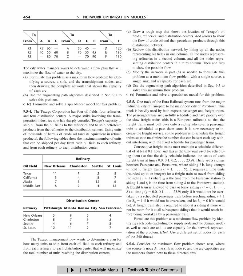
(a) Draw a rough map that shows the location of Texago’s oilfields, refineries, and distribution centers. Add arrows to showthe flow of crude oil and then petroleum products through thisdistribution network.
(b) Redraw this distribution network by lining up all the nodesrepresenting oil fields in one column, all the nodes represent-ing refineries in a second column, and all the nodes repre-senting distribution centers in a third column. Then add arcsto show the possible flow.
(c) Modify the network in part (b) as needed to formulate thisproblem as a maximum flow problem with a single source, asingle sink, and a capacity for each arc.
(d) Use the augmenting path algorithm described in Sec. 9.5 tosolve this maximum flow problem.
C (e) Formulate and solve a spreadsheet model for this problem.
9.5-5. One track of the Eura Railroad system runs from the majorindustrial city of Faireparc to the major port city of Portstown. Thistrack is heavily used by both express passenger and freight trains.The passenger trains are carefully scheduled and have priority overthe slow freight trains (this is a European railroad), so that thefreight trains must pull over onto a siding whenever a passengertrain is scheduled to pass them soon. It is now necessary to in-crease the freight service, so the problem is to schedule the freighttrains so as to maximize the number that can be sent each day with-out interfering with the fixed schedule for passenger trains.
Consecutive freight trains must maintain a schedule differen-tial of at least 0.1 hour, and this is the time unit used for schedul-ing them (so that the daily schedule indicates the status of eachfreight train at times 0.0, 0.1, 0.2, . . . , 23.9). There are S sidingsbetween Faireparc and Portstown, where siding i is long enoughto hold ni freight trains (i � 1, . . . , S ). It requires ti time units(rounded up to an integer) for a freight train to travel from sidingi to siding i � 1 (where t0 is the time from the Faireparc station tosiding 1 and ts is the time from siding S to the Portstown station).A freight train is allowed to pass or leave siding i (i � 0, 1, . . . ,S ) at time j ( j � 0.0, 0.1, . . . , 23.9) only if it would not be over-taken by a scheduled passenger train before reaching siding i � 1(let ij � 1 if it would not be overtaken, and let ij � 0 if it wouldbe). A freight train also is required to stop at a siding if there willnot be room for it at all subsequent sidings that it would reach be-fore being overtaken by a passenger train.
Formulate this problem as a maximum flow problem by iden-tifying each node (including the supply node and the demand node)as well as each arc and its arc capacity for the network represen-tation of the problem. (Hint: Use a different set of nodes for eachof the 240 times.)
9.5-6. Consider the maximum flow problem shown next, wherethe source is node A, the sink is node F, and the arc capacities arethe numbers shown next to these directed arcs.
454 9 NETWORK OPTIMIZATION MODELS
FromTo FromTo FromTo
From A B C From D E F From T
R1 75 65 — A 60 45 — D 120R2 40 50 60 B 70 55 45 E 190R3 — 80 70 C — 70 90 F 130
The city water manager wants to determine a flow plan that willmaximize the flow of water to the city.(a) Formulate this problem as a maximum flow problem by iden-
tifying a source, a sink, and the transshipment nodes, andthen drawing the complete network that shows the capacityof each arc.
(b) Use the augmenting path algorithm described in Sec. 9.5 tosolve this problem.
C (c) Formulate and solve a spreadsheet model for this problem.
9.5-4. The Texago Corporation has four oil fields, four refineries,and four distribution centers. A major strike involving the trans-portation industries now has sharply curtailed Texago’s capacity toship oil from the oil fields to the refineries and to ship petroleumproducts from the refineries to the distribution centers. Using unitsof thousands of barrels of crude oil (and its equivalent in refinedproducts), the following tables show the maximum number of unitsthat can be shipped per day from each oil field to each refinery,and from each refinery to each distribution center.
Refinery
Oil Field New Orleans Charleston Seattle St. Louis
Texas 11 7 2 8California 5 4 8 7Alaska 7 3 12 6Middle East 8 9 4 15
Distribution Center
Refinery Pittsburgh Atlanta Kansas City San Francisco
New Orleans 5 9 6 4Charleston 8 7 9 5Seattle 4 6 7 8St. Louis 12 11 9 7
The Texago management now wants to determine a plan forhow many units to ship from each oil field to each refinery andfrom each refinery to each distribution center that will maximizethe total number of units reaching the distribution centers.

9.6-4. The Makonsel Company is a fully integrated company thatboth produces goods and sells them at its retail outlets. After pro-duction, the goods are stored in the company’s two warehouses un-til needed by the retail outlets. Trucks are used to transport thegoods from the two plants to the warehouses, and then from thewarehouses to the three retail outlets.
Using units of full truckloads, the following table shows eachplant’s monthly output, its shipping cost per truckload sent to eachwarehouse, and the maximum amount that it can ship per monthto each warehouse.
(a) Use the augmenting path algorithm described inSec. 9.5 to solve this problem.
C (b) Formulate and solve a spreadsheet model forthis problem.
9.6-1. Reconsider the maximum flow problem shownin Prob. 9.5-6. Formulate this problem as a minimumcost flow problem, including adding the arc A � F.Use F� � 20.
9.6-2. A company will be producing the same new product at twodifferent factories, and then the product must be shipped to twowarehouses. Factory 1 can send an unlimited amount by rail towarehouse 1 only, whereas factory 2 can send an unlimited amountby rail to warehouse 2 only. However, independent truckers can beused to ship up to 50 units from each factory to a distribution cen-ter, from which up to 50 units can be shipped to each warehouse.The shipping cost per unit for each alternative is shown in the fol-lowing table, along with the amounts to be produced at the facto-ries and the amounts needed at the warehouses.
CHAPTER 9 PROBLEMS 455
A
B
C
D
E
F
6
9
32
4
6
7
9
7
For each retail outlet (RO), the next table shows its monthlydemand, its shipping cost per truckload from each warehouse, andthe maximum amount that can be shipped per month from eachwarehouse.
Unit Shipping Cost
To WarehouseDistribution
From Center 1 2 Output
Factory 1 3 7 — 80Factory 2 4 — 9 70
Distribution center 2 4
Allocation 60 90
(a) Formulate the network representation of this problem as a min-imum cost flow problem.
(b) Formulate the linear programming model for this problem.
9.6-3. Reconsider Prob. 9.3-1. Now formulate this problem as aminimum cost flow problem by showing the appropriate networkrepresentation.
To Unit Shipping Cost Shipping Capacity
From RO1 RO2 RO3 RO1 RO2 RO3
Warehouse 1 $470 $505 $490 100 150 100Warehouse 2 $390 $410 $440 125 150 75
Demand $150 $200 $150 150 200 150
Management now wants to determine a distribution plan(number of truckloads shipped per month from each plant to eachwarehouse and from each warehouse to each retail outlet) that willminimize the total shipping cost.(a) Draw a network that depicts the company’s distribution net-
work. Identify the supply nodes, transshipment nodes, and de-mand nodes in this network.
(b) Formulate this problem as a minimum cost flow problem byinserting all the necessary data into this network.
C (c) Formulate and solve a spreadsheet model for this problem.C (d) Use the computer to solve this problem without using Excel.
9.6-5. The Audiofile Company produces boomboxes. However,management has decided to subcontract out the production of thespeakers needed for the boomboxes. Three vendors are availableto supply the speakers. Their price for each shipment of 1,000speakers is shown on the next page.
To Unit Shipping Cost Shipping Capacity
From Warehouse 1 Warehouse 2 Warehouse 1 Warehouse 2 Output
Plant 1 $425 $560 125 150 200Plant 2 $510 $600 175 200 300
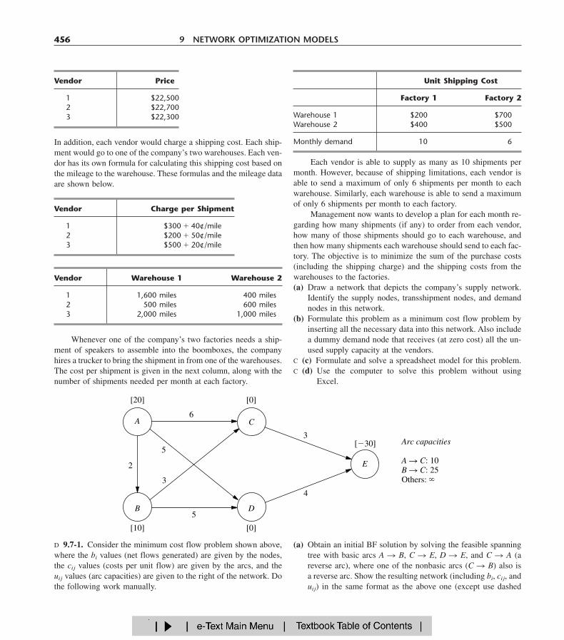
In addition, each vendor would charge a shipping cost. Each ship-ment would go to one of the company’s two warehouses. Each ven-dor has its own formula for calculating this shipping cost based onthe mileage to the warehouse. These formulas and the mileage dataare shown below.
456 9 NETWORK OPTIMIZATION MODELS
Vendor Price
1 $22,5002 $22,7003 $22,300
Vendor Charge per Shipment
1 $300 � 40¢/mile2 $200 � 50¢/mile3 $500 � 20¢/mile
Vendor Warehouse 1 Warehouse 2
1 1,600 miles 1,400 miles2 1,500 miles 1,600 miles3 2,000 miles 1,000 miles
Unit Shipping Cost
Factory 1 Factory 2
Warehouse 1 $200 $700Warehouse 2 $400 $500
Monthly demand 10 6
E
A
B
C
D
3
4
[0]
[�30]
[10]
[20] [0]
6
2
5
3
5
Arc capacities
A � C: 10B � C: 25Others:
Each vendor is able to supply as many as 10 shipments permonth. However, because of shipping limitations, each vendor isable to send a maximum of only 6 shipments per month to eachwarehouse. Similarly, each warehouse is able to send a maximumof only 6 shipments per month to each factory.
Management now wants to develop a plan for each month re-garding how many shipments (if any) to order from each vendor,how many of those shipments should go to each warehouse, andthen how many shipments each warehouse should send to each fac-tory. The objective is to minimize the sum of the purchase costs(including the shipping charge) and the shipping costs from thewarehouses to the factories.(a) Draw a network that depicts the company’s supply network.
Identify the supply nodes, transshipment nodes, and demandnodes in this network.
(b) Formulate this problem as a minimum cost flow problem byinserting all the necessary data into this network. Also includea dummy demand node that receives (at zero cost) all the un-used supply capacity at the vendors.
C (c) Formulate and solve a spreadsheet model for this problem.C (d) Use the computer to solve this problem without using
Excel.
Whenever one of the company’s two factories needs a ship-ment of speakers to assemble into the boomboxes, the companyhires a trucker to bring the shipment in from one of the warehouses.The cost per shipment is given in the next column, along with thenumber of shipments needed per month at each factory.
D 9.7-1. Consider the minimum cost flow problem shown above,where the bi values (net flows generated) are given by the nodes,the cij values (costs per unit flow) are given by the arcs, and theuij values (arc capacities) are given to the right of the network. Dothe following work manually.
(a) Obtain an initial BF solution by solving the feasible spanningtree with basic arcs A � B, C � E, D � E, and C � A (areverse arc), where one of the nonbasic arcs (C � B) also isa reverse arc. Show the resulting network (including bi, cij, anduij) in the same format as the above one (except use dashed
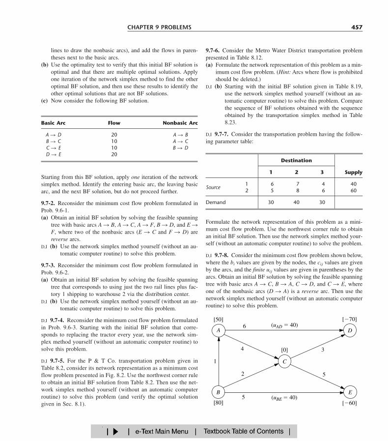
9.7-6. Consider the Metro Water District transportation problempresented in Table 8.12.(a) Formulate the network representation of this problem as a min-
imum cost flow problem. (Hint: Arcs where flow is prohibitedshould be deleted.)
D,I (b) Starting with the initial BF solution given in Table 8.19,use the network simplex method yourself (without an au-tomatic computer routine) to solve this problem. Comparethe sequence of BF solutions obtained with the sequenceobtained by the transportation simplex method in Table8.23.
D,I 9.7-7. Consider the transportation problem having the follow-ing parameter table:
lines to draw the nonbasic arcs), and add the flows in paren-theses next to the basic arcs.
(b) Use the optimality test to verify that this initial BF solution isoptimal and that there are multiple optimal solutions. Applyone iteration of the network simplex method to find the otheroptimal BF solution, and then use these results to identify theother optimal solutions that are not BF solutions.
(c) Now consider the following BF solution.
CHAPTER 9 PROBLEMS 457
Starting from this BF solution, apply one iteration of the networksimplex method. Identify the entering basic arc, the leaving basicarc, and the next BF solution, but do not proceed further.
9.7-2. Reconsider the minimum cost flow problem formulated inProb. 9.6-1.(a) Obtain an initial BF solution by solving the feasible spanning
tree with basic arcs A � B, A � C, A � F, B � D, and E �F, where two of the nonbasic arcs (E � C and F � D) arereverse arcs.
D,I (b) Use the network simplex method yourself (without an au-tomatic computer routine) to solve this problem.
9.7-3. Reconsider the minimum cost flow problem formulated inProb. 9.6-2.(a) Obtain an initial BF solution by solving the feasible spanning
tree that corresponds to using just the two rail lines plus fac-tory 1 shipping to warehouse 2 via the distribution center.
D,I (b) Use the network simplex method yourself (without an au-tomatic computer routine) to solve this problem.
D,I 9.7-4. Reconsider the minimum cost flow problem formulatedin Prob. 9.6-3. Starting with the initial BF solution that corre-sponds to replacing the tractor every year, use the network sim-plex method yourself (without an automatic computer routine) tosolve this problem.
D,I 9.7-5. For the P & T Co. transportation problem given inTable 8.2, consider its network representation as a minimum costflow problem presented in Fig. 8.2. Use the northwest corner ruleto obtain an initial BF solution from Table 8.2. Then use the net-work simplex method yourself (without an automatic computerroutine) to solve this problem (and verify the optimal solutiongiven in Sec. 8.1).
Formulate the network representation of this problem as a mini-mum cost flow problem. Use the northwest corner rule to obtainan initial BF solution. Then use the network simplex method your-self (without an automatic computer routine) to solve the problem.
D,I 9.7-8. Consider the minimum cost flow problem shown below,where the bi values are given by the nodes, the cij values are givenby the arcs, and the finite uij values are given in parentheses by thearcs. Obtain an initial BF solution by solving the feasible spanningtree with basic arcs A � C, B � A, C � D, and C � E, whereone of the nonbasic arcs (D � A) is a reverse arc. Then use thenetwork simplex method yourself (without an automatic computerroutine) to solve this problem.
Basic Arc Flow Nonbasic Arc
A � D 20 A � BB � C 10 A � CC � E 10 B � DD � E 20
Destination
1 2 3 Supply
1 6 7 4 40Source
2 5 8 6 60
Demand 30 40 30
3
5
[50]
[80]
A6 (uAD � 40)
C
[�70]
[�60]
[0]
(uBE � 40)
4
2
5
D
B E
1
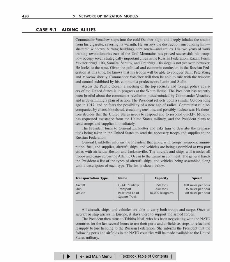
458 9 NETWORK OPTIMIZATION MODELS
Commander Votachev steps into the cold October night and deeply inhales the smokefrom his cigarette, savoring its warmth. He surveys the destruction surrounding him—shattered windows, burning buildings, torn roads—and smiles. His two years of worktraining revolutionaries east of the Ural Mountains has proved successful; his troopsnow occupy seven strategically important cities in the Russian Federation: Kazan, Perm,Yekaterinburg, Ufa, Samara, Saratov, and Orenburg. His siege is not yet over, however.He looks to the west. Given the political and economic confusion in the Russian Fed-eration at this time, he knows that his troops will be able to conquer Saint Petersburgand Moscow shortly. Commander Votachev will then be able to rule with the wisdomand control exhibited by his communist predecessors Lenin and Stalin.
Across the Pacific Ocean, a meeting of the top security and foreign policy advis-ers of the United States is in progress at the White House. The President has recentlybeen briefed about the communist revolution masterminded by Commander Votachevand is determining a plan of action. The President reflects upon a similar October longago in 1917, and he fears the possibility of a new age of radical Communist rule ac-companied by chaos, bloodshed, escalating tensions, and possibly nuclear war. He there-fore decides that the United States needs to respond and to respond quickly. Moscowhas requested assistance from the United States military, and the President plans tosend troops and supplies immediately.
The President turns to General Lankletter and asks him to describe the prepara-tions being taken in the United States to send the necessary troops and supplies to theRussian Federation.
General Lankletter informs the President that along with troops, weapons, ammu-nition, fuel, and supplies, aircraft, ships, and vehicles are being assembled at two portcities with airfields: Boston and Jacksonville. The aircraft and ships will transfer alltroops and cargo across the Atlantic Ocean to the Eurasian continent. The general handsthe President a list of the types of aircraft, ships, and vehicles being assembled alongwith a description of each type. The list is shown below.
CASE 9.1 AIDING ALLIES
Transportation Type Name Capacity Speed
Aircraft C-141 Starlifter 150 tons 400 miles per hourShip Transport 240 tons 35 miles per hourVehicle Palletized Load 16,000 kilograms 60 miles per hour
System Truck
All aircraft, ships, and vehicles are able to carry both troops and cargo. Once anaircraft or ship arrives in Europe, it stays there to support the armed forces.
The President then turns to Tabitha Neal, who has been negotiating with the NATOcountries for the last several hours to use their ports and airfields as stops to refuel andresupply before heading to the Russian Federation. She informs the President that thefollowing ports and airfields in the NATO countries will be made available to the UnitedStates military.
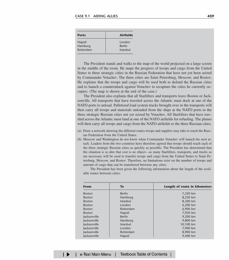
CASE 9.1 AIDING ALLIES 459
The President stands and walks to the map of the world projected on a large screenin the middle of the room. He maps the progress of troops and cargo from the UnitedStates to three strategic cities in the Russian Federation that have not yet been seizedby Commander Votachev. The three cities are Saint Petersburg, Moscow, and Rostov.He explains that the troops and cargo will be used both to defend the Russian citiesand to launch a counterattack against Votachev to recapture the cities he currently oc-cupies. (The map is shown at the end of the case.)
The President also explains that all Starlifters and transports leave Boston or Jack-sonville. All transports that have traveled across the Atlantic must dock at one of theNATO ports to unload. Palletized load system trucks brought over in the transports willthen carry all troops and materials unloaded from the ships at the NATO ports to thethree strategic Russian cities not yet seized by Votachev. All Starlifters that have trav-eled across the Atlantic must land at one of the NATO airfields for refueling. The planeswill then carry all troops and cargo from the NATO airfields to the three Russian cities.
(a) Draw a network showing the different routes troops and supplies may take to reach the Russ-ian Federation from the United States.
(b) Moscow and Washington do not know when Commander Votachev will launch his next at-tack. Leaders from the two countries have therefore agreed that troops should reach each ofthe three strategic Russian cities as quickly as possible. The President has determined thatthe situation is so dire that cost is no object—as many Starlifters, transports, and trucks asare necessary will be used to transfer troops and cargo from the United States to Saint Pe-tersburg, Moscow, and Rostov. Therefore, no limitations exist on the number of troops andamount of cargo that can be transferred between any cities.
The President has been given the following information about the length of the avail-able routes between cities:
Ports Airfields
Napoli LondonHamburg BerlinRotterdam Istanbul
From To Length of route in kilometers
Boston Berlin 7,250 kmBoston Hamburg 8,250 kmBoston Istanbul 8,300 kmBoston London 6,200 kmBoston Rotterdam 6,900 kmBoston Napoli 7,950 kmJacksonville Berlin 9,200 kmJacksonville Hamburg 9,800 kmJacksonville Istanbul 10,100 kmJacksonville London 7,900 kmJacksonville Rotterdam 8,900 kmJacksonville Napoli 9,400 km

460 9 NETWORK OPTIMIZATION MODELS
Given the distance and the speed of the transportation used between each pair of cities,how can the President most quickly move troops from the United States to each of the threestrategic Russian cities? Highlight the path(s) on the network. How long will it take troops andsupplies to reach Saint Petersburg? Moscow? Rostov?
(c) The President encounters only one problem with his first plan: he has to sell the military de-ployment to Congress. Under the War Powers Act, the President is required to consult withCongress before introducing troops into hostilities or situations where hostilities will occur.If Congress does not give authorization to the President for such use of troops, the Presidentmust withdraw troops after 60 days. Congress also has the power to decrease the 60-daytime period by passing a concurrent resolution.
The President knows that Congress will not authorize significant spending for anothercountry’s war, especially when voters have paid so much attention to decreasing the nationaldebt. He therefore decides that he needs to find a way to get the needed troops and suppliesto Saint Petersburg, Moscow, and Rostov at the minimum cost.
Each Russian city has contacted Washington to communicate the number of troops andsupplies the city needs at a minimum for reinforcement. After analyzing the requests, GeneralLankletter has converted the requests from numbers of troops, gallons of gasoline, etc., to tonsof cargo for easier planning. The requirements are listed below.
City Requirements
Saint Petersburg 320,000 tonsMoscow 440,000 tonsRostov 240,000 tons
From To Length of route in kilometers
Berlin Saint Petersburg 1,280 kmHamburg Saint Petersburg 1,880 kmIstanbul Saint Petersburg 2,040 kmLondon Saint Petersburg 1,980 kmRotterdam Saint Petersburg 2,200 kmNapoli Saint Petersburg 2,970 kmBerlin Moscow 1,600 kmHamburg Moscow 2,120 kmIstanbul Moscow 1,700 kmLondon Moscow 2,300 kmRotterdam Moscow 2,450 kmNapoli Moscow 2,890 kmBerlin Rostov 1,730 kmHamburg Rostov 2,470 kmIstanbul Rostov 990 kmLondon Rostov 2,860 kmRotterdam Rostov 2,760 kmNapoli Rostov 2,800 km
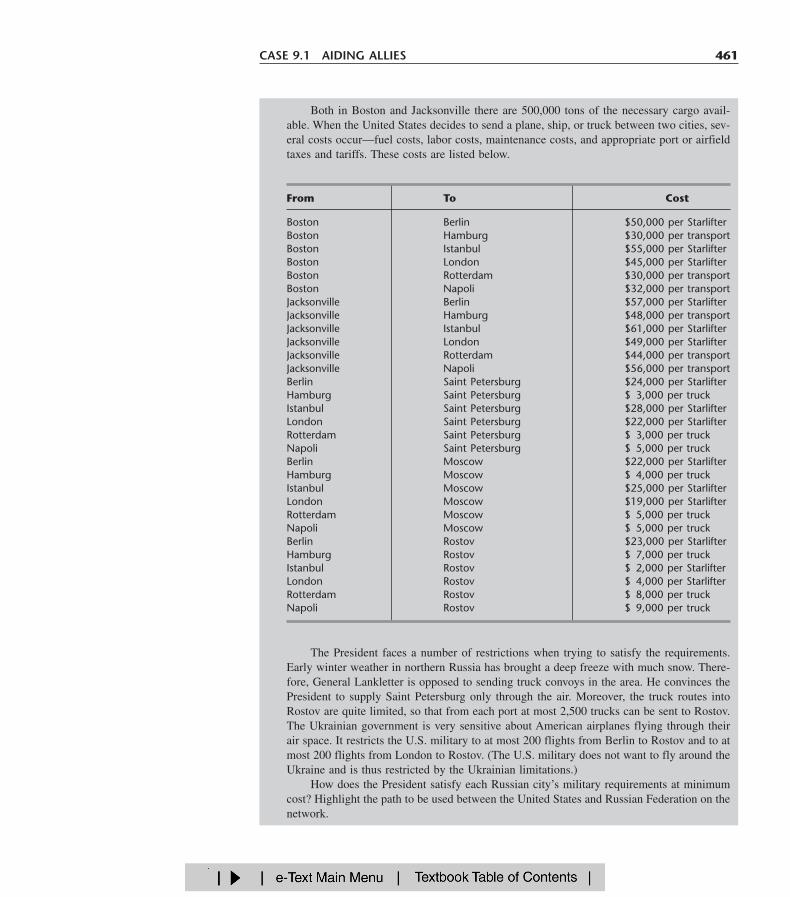
Both in Boston and Jacksonville there are 500,000 tons of the necessary cargo avail-able. When the United States decides to send a plane, ship, or truck between two cities, sev-eral costs occur—fuel costs, labor costs, maintenance costs, and appropriate port or airfieldtaxes and tariffs. These costs are listed below.
CASE 9.1 AIDING ALLIES 461
The President faces a number of restrictions when trying to satisfy the requirements.Early winter weather in northern Russia has brought a deep freeze with much snow. There-fore, General Lankletter is opposed to sending truck convoys in the area. He convinces thePresident to supply Saint Petersburg only through the air. Moreover, the truck routes intoRostov are quite limited, so that from each port at most 2,500 trucks can be sent to Rostov.The Ukrainian government is very sensitive about American airplanes flying through theirair space. It restricts the U.S. military to at most 200 flights from Berlin to Rostov and to atmost 200 flights from London to Rostov. (The U.S. military does not want to fly around theUkraine and is thus restricted by the Ukrainian limitations.)
How does the President satisfy each Russian city’s military requirements at minimumcost? Highlight the path to be used between the United States and Russian Federation on thenetwork.
From To Cost
Boston Berlin $50,000 per StarlifterBoston Hamburg $30,000 per transportBoston Istanbul $55,000 per StarlifterBoston London $45,000 per StarlifterBoston Rotterdam $30,000 per transportBoston Napoli $32,000 per transportJacksonville Berlin $57,000 per StarlifterJacksonville Hamburg $48,000 per transportJacksonville Istanbul $61,000 per StarlifterJacksonville London $49,000 per StarlifterJacksonville Rotterdam $44,000 per transportJacksonville Napoli $56,000 per transportBerlin Saint Petersburg $24,000 per StarlifterHamburg Saint Petersburg $ 3,000 per truckIstanbul Saint Petersburg $28,000 per StarlifterLondon Saint Petersburg $22,000 per StarlifterRotterdam Saint Petersburg $ 3,000 per truckNapoli Saint Petersburg $ 5,000 per truckBerlin Moscow $22,000 per StarlifterHamburg Moscow $ 4,000 per truckIstanbul Moscow $25,000 per StarlifterLondon Moscow $19,000 per StarlifterRotterdam Moscow $ 5,000 per truckNapoli Moscow $ 5,000 per truckBerlin Rostov $23,000 per StarlifterHamburg Rostov $ 7,000 per truckIstanbul Rostov $ 2,000 per StarlifterLondon Rostov $ 4,000 per StarlifterRotterdam Rostov $ 8,000 per truckNapoli Rostov $ 9,000 per truck
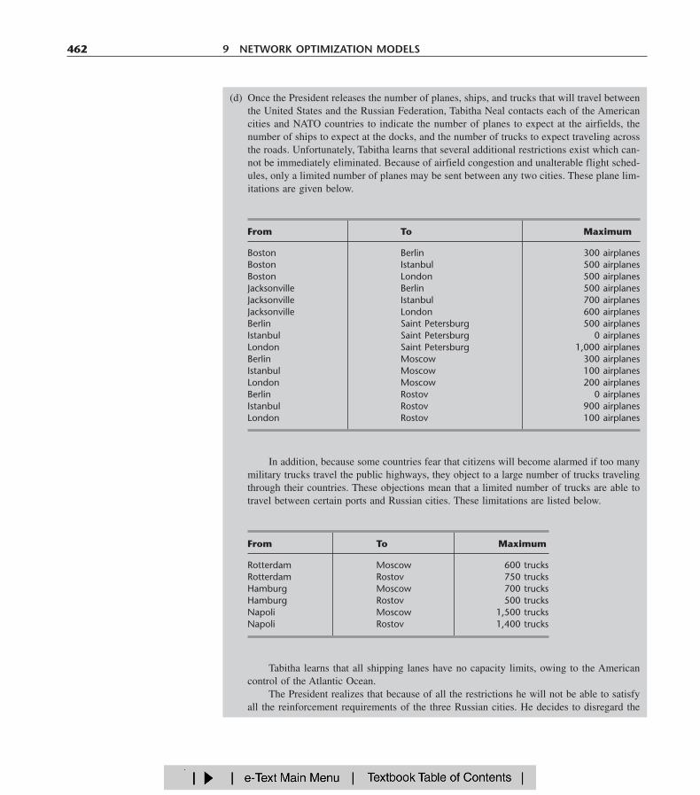
(d) Once the President releases the number of planes, ships, and trucks that will travel betweenthe United States and the Russian Federation, Tabitha Neal contacts each of the Americancities and NATO countries to indicate the number of planes to expect at the airfields, thenumber of ships to expect at the docks, and the number of trucks to expect traveling acrossthe roads. Unfortunately, Tabitha learns that several additional restrictions exist which can-not be immediately eliminated. Because of airfield congestion and unalterable flight sched-ules, only a limited number of planes may be sent between any two cities. These plane lim-itations are given below.
462 9 NETWORK OPTIMIZATION MODELS
In addition, because some countries fear that citizens will become alarmed if too manymilitary trucks travel the public highways, they object to a large number of trucks travelingthrough their countries. These objections mean that a limited number of trucks are able totravel between certain ports and Russian cities. These limitations are listed below.
From To Maximum
Rotterdam Moscow 600 trucksRotterdam Rostov 750 trucksHamburg Moscow 700 trucksHamburg Rostov 500 trucksNapoli Moscow 1,500 trucksNapoli Rostov 1,400 trucks
Tabitha learns that all shipping lanes have no capacity limits, owing to the Americancontrol of the Atlantic Ocean.
The President realizes that because of all the restrictions he will not be able to satisfyall the reinforcement requirements of the three Russian cities. He decides to disregard the
From To Maximum
Boston Berlin 300 airplanesBoston Istanbul 500 airplanesBoston London 500 airplanesJacksonville Berlin 500 airplanesJacksonville Istanbul 700 airplanesJacksonville London 600 airplanesBerlin Saint Petersburg 500 airplanesIstanbul Saint Petersburg 0 airplanesLondon Saint Petersburg 1,000 airplanesBerlin Moscow 300 airplanesIstanbul Moscow 100 airplanesLondon Moscow 200 airplanesBerlin Rostov 0 airplanesIstanbul Rostov 900 airplanesLondon Rostov 100 airplanes
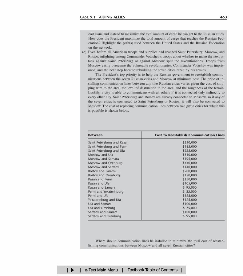
cost issue and instead to maximize the total amount of cargo he can get to the Russian cities.How does the President maximize the total amount of cargo that reaches the Russian Fed-eration? Highlight the path(s) used between the United States and the Russian Federationon the network.
(e) Even before all American troops and supplies had reached Saint Petersburg, Moscow, andRostov, infighting among Commander Votachev’s troops about whether to make the next at-tack against Saint Petersburg or against Moscow split the revolutionaries. Troops fromMoscow easily overcame the vulnerable revolutionaries. Commander Votachev was impris-oned, and the next step became rebuilding the seven cities razed by his armies.
The President’s top priority is to help the Russian government to reestablish commu-nications between the seven Russian cities and Moscow at minimum cost. The price of in-stalling communication lines between any two Russian cities varies given the cost of ship-ping wire to the area, the level of destruction in the area, and the roughness of the terrain.Luckily, a city is able to communicate with all others if it is connected only indirectly toevery other city. Saint Petersburg and Rostov are already connected to Moscow, so if any ofthe seven cities is connected to Saint Petersburg or Rostov, it will also be connected toMoscow. The cost of replacing communication lines between two given cities for which thisis possible is shown below.
CASE 9.1 AIDING ALLIES 463
Where should communication lines be installed to minimize the total cost of reestab-lishing communications between Moscow and all seven Russian cities?
Between Cost to Reestablish Communication Lines
Saint Petersburg and Kazan $210,000Saint Petersburg and Perm $185,000Saint Petersburg and Ufa $225,000Moscow and Ufa $310,000Moscow and Samara $195,000Moscow and Orenburg $440,000Moscow and Saratov $140,000Rostov and Saratov $200,000Rostov and Orenburg $120,000Kazan and Perm $150,000Kazan and Ufa $105,000Kazan and Samara $ 95,000Perm and Yekaterinburg $ 85,000Perm and Ufa $125,000Yekaterinburg and Ufa $125,000Ufa and Samara $100,000Ufa and Orenburg $ 75,000Saratov and Samara $100,000Saratov and Orenburg $ 95,000
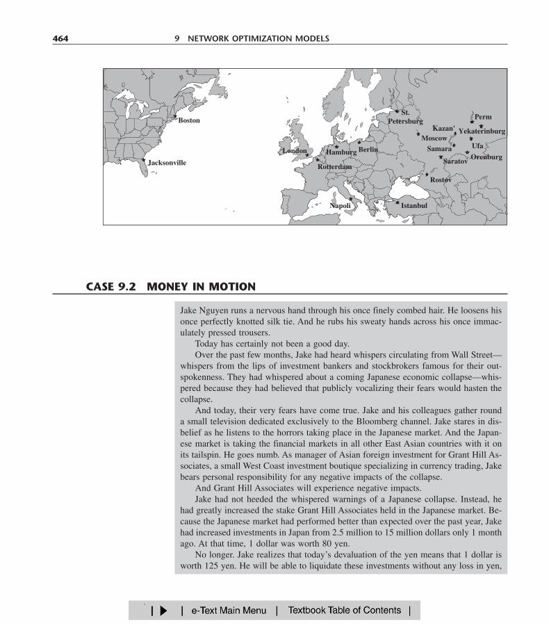
464 9 NETWORK OPTIMIZATION MODELS
Jake Nguyen runs a nervous hand through his once finely combed hair. He loosens hisonce perfectly knotted silk tie. And he rubs his sweaty hands across his once immac-ulately pressed trousers.
Today has certainly not been a good day.Over the past few months, Jake had heard whispers circulating from Wall Street—
whispers from the lips of investment bankers and stockbrokers famous for their out-spokenness. They had whispered about a coming Japanese economic collapse—whis-pered because they had believed that publicly vocalizing their fears would hasten thecollapse.
And today, their very fears have come true. Jake and his colleagues gather rounda small television dedicated exclusively to the Bloomberg channel. Jake stares in dis-belief as he listens to the horrors taking place in the Japanese market. And the Japan-ese market is taking the financial markets in all other East Asian countries with it onits tailspin. He goes numb. As manager of Asian foreign investment for Grant Hill As-sociates, a small West Coast investment boutique specializing in currency trading, Jakebears personal responsibility for any negative impacts of the collapse.
And Grant Hill Associates will experience negative impacts.Jake had not heeded the whispered warnings of a Japanese collapse. Instead, he
had greatly increased the stake Grant Hill Associates held in the Japanese market. Be-cause the Japanese market had performed better than expected over the past year, Jakehad increased investments in Japan from 2.5 million to 15 million dollars only 1 monthago. At that time, 1 dollar was worth 80 yen.
No longer. Jake realizes that today’s devaluation of the yen means that 1 dollar isworth 125 yen. He will be able to liquidate these investments without any loss in yen,
CASE 9.2 MONEY IN MOTION
Yekaterinburg
St.Petersburg
Perm
UfaMoscow
Boston
Jacksonville
BerlinLondon
Napoli Istanbul
Rostov
SaratovOrenburg
Samara
Kazan'
Hamburg
Rotterdam

CASE 9.2 MONEY IN MOTION 465
but now the dollar loss when converting back into U.S. currency would be huge. Hetakes a deep breath, closes his eyes, and mentally prepares himself for serious damagecontrol.
Jake’s meditation is interrupted by a booming voice calling for him from a largecorner office. Grant Hill, the president of Grant Hill Associates, yells, “Nguyen, getthe hell in here!”
Jake jumps and looks reluctantly toward the corner office hiding the furious GrantHill. He smooths his hair, tightens his tie, and walks briskly into the office.
Grant Hill meets Jake’s eyes upon his entrance and continues yelling, “I don’t wantone word out of you, Nguyen! No excuses; just fix this debacle! Get all of our moneyout of Japan! My gut tells me this is only the beginning! Get the money into safe U.S.bonds! NOW! And don’t forget to get our cash positions out of Indonesia and MalaysiaASAP with it!”
Jake has enough common sense to say nothing. He nods his head, turns on his heel,and practically runs out of the office.
Safely back at his desk, Jake begins formulating a plan to move the investmentsout of Japan, Indonesia, and Malaysia. His experiences investing in foreign marketshave taught him that when playing with millions of dollars, how he gets money out ofa foreign market is almost as important as when he gets money out of the market. Thebanking partners of Grant Hill Associates charge different transaction fees for con-verting one currency into another one and wiring large sums of money around the globe.
And now, to make matters worse, the governments in East Asia have imposed verytight limits on the amount of money an individual or a company can exchange fromthe domestic currency into a particular foreign currency and withdraw it from the coun-try. The goal of this dramatic measure is to reduce the outflow of foreign investmentsout of those countries to prevent a complete collapse of the economies in the region.Because of Grant Hill Associates’ cash holdings of 10.5 billion Indonesian rupiahs and28 million Malaysian ringgits, along with the holdings in yen, it is not clear how theseholdings should be converted back into dollars.
Jake wants to find the most cost-effective method to convert these holdings intodollars. On his company’s website he always can find on-the-minute exchange ratesfor most currencies in the world (Table 1).
The table states that, for example, 1 Japanese yen equals 0.008 U.S. dollars. Bymaking a few phone calls he discovers the transaction costs his company must pay forlarge currency transactions during these critical times (Table 2).
Jake notes that exchanging one currency for another one results in the same trans-action cost as a reverse conversion. Finally, Jake finds out the maximum amounts ofdomestic currencies his company is allowed to convert into other currencies in Japan,Indonesia, and Malaysia (Table 3).
(a) Formulate Jake’s problem as a minimum cost flow problem, and draw the network for hisproblem. Identify the supply and demand nodes for the network.
(b) Which currency transactions must Jake perform in order to convert the investments fromyen, rupiah, and ringgit into U.S. dollars to ensure that Grant Hill Associates has the max-imum dollar amount after all transactions have occurred? How much money does Jake haveto invest in U.S. bonds?
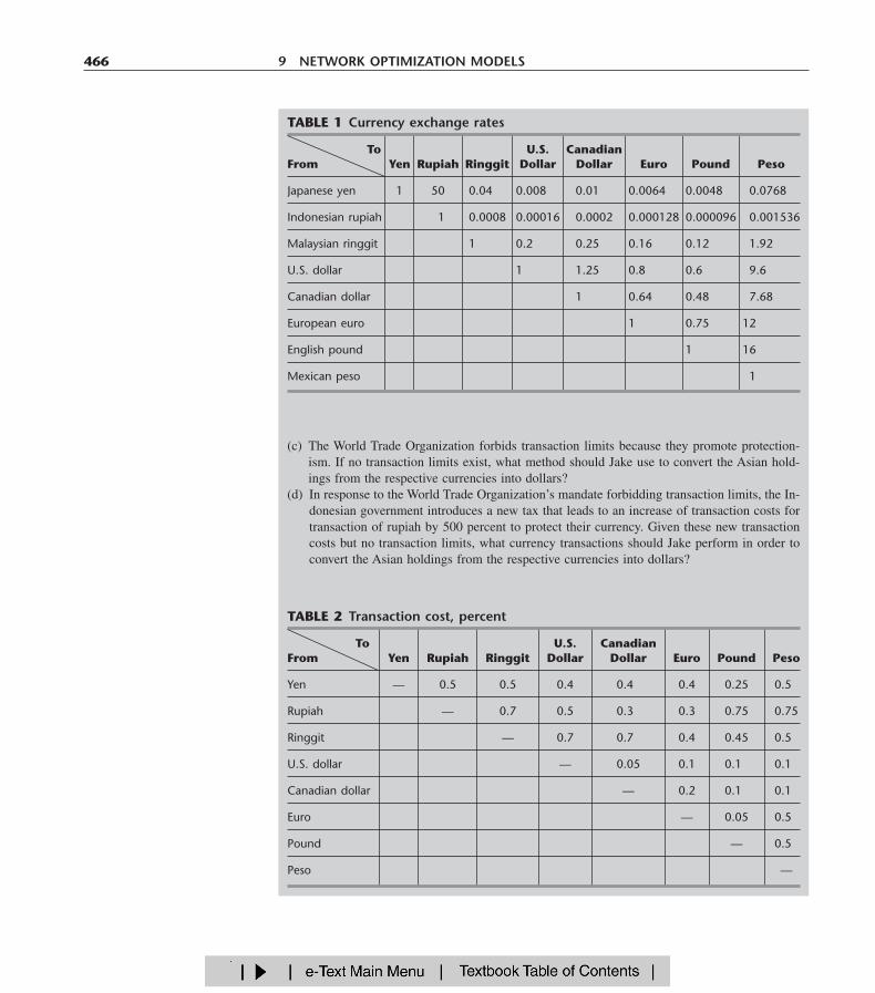
(c) The World Trade Organization forbids transaction limits because they promote protection-ism. If no transaction limits exist, what method should Jake use to convert the Asian hold-ings from the respective currencies into dollars?
(d) In response to the World Trade Organization’s mandate forbidding transaction limits, the In-donesian government introduces a new tax that leads to an increase of transaction costs fortransaction of rupiah by 500 percent to protect their currency. Given these new transactioncosts but no transaction limits, what currency transactions should Jake perform in order toconvert the Asian holdings from the respective currencies into dollars?
466 9 NETWORK OPTIMIZATION MODELS
TABLE 1 Currency exchange rates
To U.S. CanadianFrom Yen Rupiah Ringgit Dollar Dollar Euro Pound Peso
Japanese yen 1 50 0.04 0.008 0.01 0.0064 0.0048 0.0768
Indonesian rupiah 1 0.0008 0.00016 0.0002 0.000128 0.000096 0.001536
Malaysian ringgit 1 0.2 0.25 0.16 0.12 1.92
U.S. dollar 1 1.25 0.8 0.6 9.6
Canadian dollar 1 0.64 0.48 7.68
European euro 1 0.75 12
English pound 1 16
Mexican peso 1
TABLE 2 Transaction cost, percent
To U.S. CanadianFrom Yen Rupiah Ringgit Dollar Dollar Euro Pound Peso
Yen — 0.5 0.5 0.4 0.4 0.4 0.25 0.5
Rupiah — 0.7 0.5 0.3 0.3 0.75 0.75
Ringgit — 0.7 0.7 0.4 0.45 0.5
U.S. dollar — 0.05 0.1 0.1 0.1
Canadian dollar — 0.2 0.1 0.1
Euro — 0.05 0.5
Pound — 0.5
Peso —
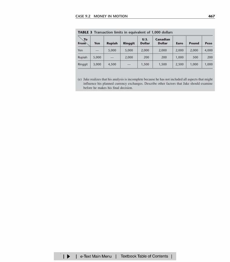
(e) Jake realizes that his analysis is incomplete because he has not included all aspects that mightinfluence his planned currency exchanges. Describe other factors that Jake should examinebefore he makes his final decision.
CASE 9.2 MONEY IN MOTION 467
TABLE 3 Transaction limits in equivalent of 1,000 dollars
To U.S. CanadianFrom Yen Rupiah Ringgit Dollar Dollar Euro Pound Peso
Yen — 5,000 5,000 2,000 2,000 2,000 2,000 4,000
Rupiah 5,000 — 2,000 200 200 1,000 500 200
Ringgit 3,000 4,500 — 1,500 1,500 2,500 1,000 1,000