chapte r the data of macroeconomics -...
TRANSCRIPT
Notes to the Instructor
Chapter SummaryChapter 2 is a straightforward chapter on economic data that emphasizes real GDP, theconsumer price index, and the unemployment rate. This chapter contains a standarddiscussion of GDP and its components, explains the different measures of inflation, and dis-cusses how the population is divided among the employed, the unemployed, and those not inthe labor force. This chapter also introduces the circular flow and the relationship betweenGDP and unemployment (Okun’s law).
CommentsStudents may have seen this material in principles classes, so it can often be coveredquickly. I prefer not to get involved in the details of national income accounting; my aim is toget students to understand the sort of issues that arise in looking at economic data and toknow where to look if and when they need more information. From the point of view of therest of the course, the most important things for students to learn are the identity of incomeand output, the distinction between real and nominal variables, and the relationshipbetween stocks and flows.
Use of the Web SiteThe discussion of economic data can be made more interesting by encouraging students touse the data plotter and look at the series being discussed. In using the software, thestudents should be encouraged to look at the data early, in order to try to familiarize themwith the basic stylized facts. The transform data option on the plotter can be used to help thestudents gain an understanding of growth rates and percentage changes, show them thedistinction between real and nominal GDP, and illustrate Okun’s law.
Use of the Dismal Scientist Web SiteUse the Dismal Scientist Web site to download data for the past 40 years on nominal GDPand the components of spending (consumption, investment, government purchases, exports,and imports). Compute the shares of spending accounted for by each component. Discusshow the shares have changed over time.
Chapter SupplementsThis chapter includes the following supplements:
2-1 Measuring Output
2-2 Pitfalls in National Income Accounting
2-3 Nominal and Real GDP Since 1929
2-4 Chain-Weight Real GDP
2-5 The Increasing Role of Services
2-6 The Components of GDP (Case Study p. 28)
13
C H A P T E R
T h e D a t a o f M a c r o e c o n o m i c s2
Full file at http://TestbankCollege.eu/Solution-Manual-Macroeconomics-7th-Edition-Gregory-Mankiw

2-7 Defining National Income
2-8 Seasonal Adjustment and the Seasonal Cycle
2-9 Measuring the Price of Light (Case Study p. 35)
2-10 Improving the CPI (Case Study p. 35)
2-11 CPI Improvements and the Decline in Inflation During the 1990s (Case Study p. 35)
2-12 Alternative Measures of Unemployment
2-13 Improving the National Accounts
14 CHAPTER 2 The Data of Macroeconomics
Full file at http://TestbankCollege.eu/Solution-Manual-Macroeconomics-7th-Edition-Gregory-Mankiw

Lecture Notes
IntroductionAn immense amount of economic data is gathered on a regular basis. Every day,newspapers, radio, and television inform us about some economic statistic or other.Although we cannot discuss all these data here, it is important to be familiar withsome of the most important measures of economic performance.
2-1 Measuring the Value of Economic Activity: Gross Domestic Product
The single most important measure of overall economic performance is GrossDomestic Product (GDP). The GDP is an attempt to summarize all economicactivity over a period of time in terms of a single number; it is a measure of theeconomy’s total output and of total income. Macroeconomists use the terms“output” and “income” interchangeably, which seems somewhat mysterious. Thereason is that, for the economy as a whole, total production equals total income.Our first task is to explain why.
Income, Expenditure, and the Circular FlowSuppose that the economy produces just one good—bread—using labor only. (Noticewhat we are doing here: we are making simplifying assumptions that are obviouslynot literally true in order to gain insight into the working of the economy.) Weassume that there are two sorts of economic actors—households and firms(bakeries). Firms hire workers from the households in order to produce bread, andpay wages to those households. Workers take those wages and purchase bread fromthe firms. These transactions take place in two markets—the goods market and thelabor market.
GDP is measured by looking at the flow of dollars in this economy. Thecircular flow of income indicates that we can think of two ways of measuring thisflow—by adding up all incomes or by adding up all expenditures. The two will haveto be equal simply by the rules of accounting. Every dollar that a firm receives forbread either goes to pay expenses or else increases profit. In our example, expensessimply consist of wages. Total expenditure thus equals the sum of wages and profit.
FYI: Stocks and FlowsGoods are not produced instantaneously—production takes time. Therefore, wemust have a period of time in mind when we think about GDP. For example, it doesnot make sense to say a bakery produces 2,000 loaves of bread. If it produces thatmany in a day, then it produces 4,000 in 2 days, 10,000 in a (5-day) week, and about130,000 in a quarter. Because we always have to keep a time dimension in mind, wesay that GDP is a flow. If we measured GDP at any tiny instant of time, it would bealmost zero.
Other variables can be measured independent of time—we refer to these asstocks. For example, economists pay a lot of attention to the factories and machinesthat firms use to produce goods. This is known as the capital stock. In principle, youcould measure this at any instant of time. Over time this capital stock will changebecause firms purchase new factories and machines. This change in the stock iscalled investment; it is a flow. Flows are changes in stocks; stocks change as a resultof flows. In understanding the macroeconomy, it is often crucial to keep thedistinction between stocks and flows in mind. A classic example of the stock–flowrelationship is that of water flowing into a bathtub.
Lecture Notes 15
➤ Figure 2-1
➤ Supplement 2-1,“Measuring Output”
➤ Figure 2-2
Full file at http://TestbankCollege.eu/Solution-Manual-Macroeconomics-7th-Edition-Gregory-Mankiw
Rules for Computing GDPNaturally, the measurement of GDP in the economy is much more complicated inpractice than our simple bread example suggests. There are any number oftechnical details of GDP measurement, which we ignore, but a few important pointsshould be mentioned.
First, what happens if a firm produces a good but does not sell it? What doesthis mean for GDP? If the good is thrown out, it is as if it were never produced. Ifone fewer loaf of bread is sold, then both expenditure and profits are lower. This isappropriate, since we would not want GDP to measure wasted goods. Alternatively,the bread may be put into inventory to be sold later. Then the rules of accountingspecify that it is as if the firm purchases the bread from itself. Both expenditureand profit are the same as if the bread were sold immediately.
Second, what about the obvious fact that there is more than one good in theeconomy? We add up different commodities by valuing them at their market price.For each commodity, we take the number produced and multiply by the price perunit. Adding this over all commodities gives us total GDP.
Many goods are intermediate goods—they are not consumed for their own sakebut are used in the production of other goods. Sheet metal is used in the productionof cars; beef is used in the production of hamburgers. The GDP statistics includeonly final goods. If a miller produces flour and sells that flour to a baker, then onlythe final sale of bread is included in GDP. An alternative but equivalent way ofmeasuring GDP is to add up the value added at all stages of production. The valueadded of the miller is the difference between the value of output (flour) and thevalue of intermediate goods (wheat). The sum of the value added at each stage ofproduction equals the value of the final output.
Finally, we need to take account of the fact that not all goods and services aresold in the marketplace. To include such goods it is necessary to calculate animputed value. An important example is owner-occupied housing. Since rentpayments to landlords are included in GDP, it would be inconsistent not to includethe equivalent housing services that homeowners enjoy. It is thus necessary toimpute a value of housing services, which is simply like supposing that homeownerspay rent to themselves. Imputed values are also calculated for the services of publicservants; they are simply valued by the wages that they are paid.
Real GDP versus Nominal GDPValuing goods at their market price allows us to add different goods into acomposite measure, but also means we might be misled into thinking we areproducing more if prices are rising. Thus, it is important to correct for changes inprices. To do this, economists value goods at the prices at which they sold at insome given year. For example, we might measure GDP at 1998 prices (oftenreferred to as measuring GDP in 1998 dollars). This is then known as real GDP.GDP measured at current prices (in current dollars) is known as nominal GDP.The distinction between real and nominal variables arises time and again inmacroeconomics.
The GDP DeflatorThe GDP deflator is the ratio of nominal to real GDP:
GDP Deflator =
The GDP deflator measures the price of output relative to prices in the base year,which we denote by P. Hence, nominal GDP equals PY.
Nominal GDPReal GDP
16 CHAPTER 2 The Data of Macroeconomics
➤ Supplement 2-2,“Pitfalls in NationalIncome Accounting”
➤ Supplement 2-3,“Nominal and RealGDP Since 1929”
Full file at http://TestbankCollege.eu/Solution-Manual-Macroeconomics-7th-Edition-Gregory-Mankiw
Chain-Weighted Measures of Real GDPIn 1996, the Bureau of Economic Analysis changed its approach to indexing GDP.Instead of using a fixed base year for prices, the Bureau began using a movingbase year. Previously, the Bureau used prices in a given year—say, 1990—tomeasure the value of goods produced in all years. Now, to measure the change inreal GDP from, say, 1995 to 1996, the Bureau uses the prices in both 1995 and1996. To measure the change in real GDP from 1996 to 1997, prices in 1996 and1997 are used.
FYI: Two Arithmetic Tricks for Working With PercentageChangesThe percentage change of a product in two variables equals (approximately) thesum of the percentage changes in the individual variables. The percentage changeof the ratio of two variables equals (approximately) the difference between the per-centage change in the numerator and the percentage change in the denominator.
The Components of ExpenditureAlthough GDP is the most general measure of output, we also care about what thisoutput is used for. National income accounts thus divide total expenditure into fourcategories, corresponding approximately to who does the spending, in an equationknown as the national income identity,
Y = C + I + G + NX,
where C is consumption, I is investment, G is government purchases, and NX is netexports, or exports minus imports. Consumption is expenditure on goods andservices by households; it is thus the spending that individuals carry out every dayon food, clothes, movies, VCRs, automobiles, and the like. Food, clothing, and othergoods that last for short periods of time are classified as nondurable goods, whereasautomobiles, VCRs, and similar goods are classified as durable goods. (Thedistinction is somewhat arbitrary: A good pair of hiking boots might last for manyyears while the latest laptop computer might be out of date in a matter of months!)There is also a third category of consumption, known as services; this is thepurchase of the time of individuals, such as doctors, lawyers, and brokers.
Investment is for the most part expenditure by firms on factories andmachinery; this is known as business fixed investment. We noted earlier that goodsput into inventory by firms are counted as part of expenditure; they are classified asinventory investment. This can be negative if firms are running down their stocks ofinventory rather than increasing them. A third component of investment spendingis actually carried out by households and landlords—residential fixed investment.This is the purchase of new housing.
The third category of expenditure corresponds to purchases by government (atall levels—federal, state, and local). It includes, most notably, defense expenditures,as well as spending on highways, bridges, and so forth. It is important to realizethat it includes only spending on goods and services that make up GDP. This meansthat it excludes unemployment insurance payments, Social Security payments, andother transfer payments. When the government pays transfers to individuals, thereis an indirect effect on GDP only, to the extent that individuals take those transferpayments and use them for consumption.
Finally, some of the goods that we produce are purchased by foreigners.These purchases represent another component of spending—exports—that mustbe added in. But, conversely, expenditures on goods produced in other countriesdo not represent purchases of goods that we produce. Since the idea of GDP is tomeasure total production in our country, imports must be subtracted. Netexports simply equal exports minus imports.
Lecture Notes 17
➤ Supplement 2-4,“Chain-Weight Real GDP”
➤ Supplement 7-5,“Growth Rates,Logarithms, andElasticities”
➤ Supplement 2-5,“The IncreasingRole of Services”
Full file at http://TestbankCollege.eu/Solution-Manual-Macroeconomics-7th-Edition-Gregory-Mankiw
FYI: What Is Investment?Economists use the term “investment” in a very precise sense. To the economist,investment means the purchase of newly created goods and services to add to thecapital stock. It does not apply to the purchase of already existing assets, since thissimply changes the ownership of the capital stock.
Case Study: GDP and Its ComponentsFor the year 2007, U.S. GDP equaled about $13.8 trillion, or $45,707 per person.Approximately 70 percent of GDP was spent on consumption (about $9.7 trillion).Private investment was about 15 percent of GDP ($2.1 trillion), while governmentpurchases were nearly 20 percent of GDP ($2.7 trillion). Imports exceeded exportsin 2000 by $708 billion.
Other Measures of IncomeThere are other measures of income apart from GDP. The most important are as fol-lows: gross national product (GNP) equals GDP minus income earned domesticallyby foreign nationals plus income earned by U.S. nationals in other countries; netnational product (NNP) equals GNP minus a correction for the depreciation or wearand tear of the capital stock (capital consumption allowance). The capital consump-tion allowance equals about 10 percent of GNP. Net national product is approxi-mately equal to national income. The two measures differ by a small amount knownas the statistical discrepancy, which reflects differences in data sources that are notcompletely consistent. By adding dividends, transfer payments, and personal inter-est income and subtracting indirect business taxes, corporate profits, social insur-ance contributions, and net interest, we move from national income to personalincome. Finally, if we subtract income taxes and nontax payments, we obtain dispos-able personal income. This is a measure of the after-tax income of consumers. Most ofthe differences among these measures of income are not important for our theoreticalmodels, but we do make use of the distinction between GDP and disposable income.
Seasonal AdjustmentMany economic variables exhibit a seasonal pattern—for example, GDP is lowest inthe first quarter of the year and highest in the last quarter. Such fluctuations arenot surprising since some sectors of the economy, such as construction, agriculture,and tourism, are influenced by the weather and the seasons. For this reason,economists often correct for such seasonal variation and look at data that areseasonally adjusted.
2-2 Measuring the Cost of Living: The Consumer Price IndexWe noted earlier the difference between real and nominal GDP: Real GDP takes GDPmeasured in dollars—nominal GDP—and adjusts for inflation. There are two basicmeasures of the inflation rate: the GDP deflator and the consumer price index (CPI).
The Price of a Basket of GoodsThe consumer price index is a good measure of inflation as it affects the typicalhousehold. It is calculated on the basis of a typical “basket of goods,” based on asurvey of consumers’ purchases. The point of having a basket of goods is that pricechanges are weighted according to how important the good is for a typicalconsumer. If the price of bread doubles, that will have a bigger effect on consumersthan if the price of matches doubles because consumers spend more of their incomeon bread than they do on matches. The CPI is defined as
18 CHAPTER 2 The Data of Macroeconomics
Supplement 3-4,“Economists’Terminology”
Table 2-1
➤
➤
Supplement 2-6,“The Components ofGDP”
Supplement 2-7,“Defining NationalIncome”
➤
➤
➤ Supplement 2-8,“Seasonal Adjust-ment and theSeasonal Cycle”
➤ Figure 2-3
Full file at http://TestbankCollege.eu/Solution-Manual-Macroeconomics-7th-Edition-Gregory-Mankiw
CPI = .
Like the GDP deflator, the CPI is a measure of the price level P. Again, thisinterpretation means that we are letting Pbase year = 1.
The CPI versus the GDP DeflatorThe GDP deflator is a measure of the price of all goods produced in the UnitedStates that go into GDP. In particular, the GDP deflator accounts for changes in theprice of investment goods and goods purchased by the government, which are notincluded in the CPI. It is, thus, a good measure of the price of “a unit of GDP.” TheCPI is a poorer measure of the price of GDP, but provides a better measure of theprice level as it affects the average consumer. Since the CPI measures the cost of atypical set of consumer purchases, it does not include the prices of, say,earthmoving equipment or Stealth bombers. It does include the prices of importedgoods that consumers purchase, such as Japanese televisions. Both of these factorsmake the CPI differ from the GDP deflator.
A final difference between these two measures of inflation is more subtle. TheCPI is calculated on the basis of a fixed basket of goods, whereas the GDP deflatoris based on a changing basket of goods. For example, when the price of apples risesand consumers purchase more oranges and fewer apples, the CPI does not take intoaccount the change in quantities purchased and continues to weight the prices ofapples and oranges by the quantities that were purchased during the base year.The GDP deflator, by contrast, weights the prices of apples and oranges by thequantities purchased in the current year. Thus, the CPI “overweights” productswhose prices are rising rapidly and “underweights” products whose prices are risingslowly, thereby overstating the rate of inflation. By using quantity weights basedon purchases in the current year, the GDP deflator captures the tendency ofconsumers to substitute away from more expensive goods and toward cheapergoods. The GDP deflator, however, may actually understate the rate of inflationbecause people may be worse off when they substitute away from goods that theyreally enjoy—someone who likes apples much better than oranges may be unhappyeating fewer apples and more oranges when the price of apples rises.
Case Study: Does the CPI Overstate Inflation?Many economists believe that changes in the CPI are an overestimate of the trueinflation rate. We already noted that the CPI overstates inflation becauseconsumers substitute away from more expensive goods. There are two otherconsiderations.
• New Goods When producers introduce a new good, consumers have morechoices, and can make better use of their dollars to satisfy their wants. Eachdollar will, in effect, buy more for an individual, so the introduction of newgoods is like a decrease in the price level. This value of greater variety is notmeasured by the CPI.
• Quality Improvements Likewise, an improvement in the quality of goods meansthat each dollar effectively buys more for the consumer. An increase in the priceof a product thus may reflect an improvement in quality and not simply a rise incost of the “same” product. The Bureau of Labor Statistics makes adjustmentsfor quality in measuring price increases for some products, including autos, butmany changes in quality are hard to measure. Accordingly, if over time thequality of products and services tends to improve rather than deteriorate, thenthe CPI probably overstates inflation.
A panel of economists recently studied the problem and concluded the CPIoverstates inflation by about 1.1 percentage points per year. The BLS has sincemade further changes in the way the CPI is calculated so that the bias is nowbelieved to be less than 1 percentage point.
Current Price of Base-Year Basket of Goods
Base-Year Price of Base-Year Basket of Goods
Lecture Notes 19
➤ Figure 2-3
➤ Supplement 2-9,“Measuring thePrice of Light”
➤ Supplement 2-10,“Improving the CPI”
➤ Supplement 2-11,“CPI Improvementsand the Decline inInflation During the1990s”
Full file at http://TestbankCollege.eu/Solution-Manual-Macroeconomics-7th-Edition-Gregory-Mankiw
2-3 Measuring Joblessness: The Unemployment RateFinally, we consider the measurement of unemployment. Employment andunemployment statistics are among the most watched of all economic data, for acouple of reasons. First, a well-functioning economy will use all its resources.Unemployment may signal wasted resources and, hence, problems in thefunctioning of the economy. Second, unemployment is often felt to be of concernsince its costs are very unevenly distributed across the population.
The Household SurveyThe U.S. Bureau of Labor Statistics calculates the unemployment rate and otherstatistics that economists and policymakers use to gauge the state of the labormarket. These statistics are based on results from the Current Population Survey ofabout 60,000 households that the Bureau performs each month. The surveyprovides estimates of the number of people in the adult population (16 years andolder) who are classified as either employed, unemployed, or not in the labor force:
POP = E + U + NL,
where POP is the population, E is the employed, U is the unemployed, and NL isthose not in the labor force. Thus, we have
L = E + U,
where L is the labor force. The labor-force participation rate is the fraction of thepopulation in the labor force:
Labor-Force Participation Rate = L/POP.
The employment rate (e) and unemployment rate (u) are given by
e = E/Lu = U/L = 1 – e.
Case Study: Trends in Labor-Force ParticipationOver the past half century, labor-force participation among women has risensharply, from 33 percent to 59 percent, while among men it has declined from 87percent to 73 percent. Many factors have contributed to the increase in women’sparticipation, including new technologies such as clothes-washing machines,dishwashers, refrigerators, etc., which reduced the time needed for householdchores, fewer children per family, and changing social and political attitudes towardwomen in the work force. For men, the decline has been due to earlier and longerperiods of retirement, more time spent in school (and out of the labor force) foryounger men, and greater prevalence of stay-at-home fathers. Some economistspredict that labor force participation will decline over coming decades as the elderlyshare of the population rises.
The Establishment SurveyIn addition to asking households about their employment status, the Bureau ofLabor Statistics also separately asks business establishments about the number ofworkers on their payroll each month. This establishment survey covers 160,000businesses that employ over 40 million workers. The survey collects data onemployment, hours worked, and wages, and provides breakdowns by industry andjob categories. Employment as measured by the establishment survey differs fromemployment as measured by the household survey for several reasons. First, a self-employed person is reported as working in the household survey but does not showup on the payroll of a business establishment and so is not counted in theestablishment survey. Second, the household survey does not count separate jobsbut only reports if a person is working, whereas the establishment survey counts
20 CHAPTER 2 The Data of Macroeconomics
➤ Figure 2-4
➤ Supplement 2-12,“AlternativeMeasures ofUnemployment”
➤ Supplement 7-6,“Labor ForceParticipation”
➤ Figure 2-5
Full file at http://TestbankCollege.eu/Solution-Manual-Macroeconomics-7th-Edition-Gregory-Mankiw
each and every job. Third, both surveys use statistical methods to extrapolate fromthe sample to the population. For the establishment survey, estimates about thenumber of workers at new start-up firms that are not yet in the sample may beimperfect. For the household survey, incorrect estimates about the overall size ofthe population—due, for example, to difficulty measuring changes in immigration—may lead to incorrect estimates of overall employment.
2-4 Conclusion: From Economic Statistics to Economic ModelsThis chapter has explained the measurement of real GDP, price indexes, andunemployment. These are important economic statistics, since they provide anindication of the overall health of the economy. The task of macroeconomics,however, is not just to describe the data and measure economic performance butalso to explain the behavior of the economy. This is the subject of our subsequentanalyses.
Lecture Notes 21
➤ Supplement 2-13,“Improving theNational Accounts”
Full file at http://TestbankCollege.eu/Solution-Manual-Macroeconomics-7th-Edition-Gregory-Mankiw

22
L E C T U R E S U P P L E M E N T
2-1 Measuring OutputAs discussed in the text, we can measure the value of national output either by adding up allof the spending on the economy’s output of goods and services or by adding up all of theincomes generated in producing output. This basic equivalence between output and incomeallows us to develop the national income accounting identities relating saving, investment,and net exports that are presented in Chapters 3 and 5.
Although the text uses the term Gross Domestic Product (GDP) to refer to both thespending measure and the income measure of total output, the national income accounts infact provide two separate measures of total output. In the national income accounts, GDP ismeasured by adding up spending on domestically produced goods and services. A separatequantity, known as Gross Domestic Income (GDI), is measured by adding up incomegenerated producing domestic output. In theory, these measures should be the same. Inpractice, however, a measurement error—known as the statistical discrepancy—means thatGDP and GDI usually differ by a small amount. Typically, the discrepancy averages close tozero over longer periods of time and tends to become smaller as the data are revised.
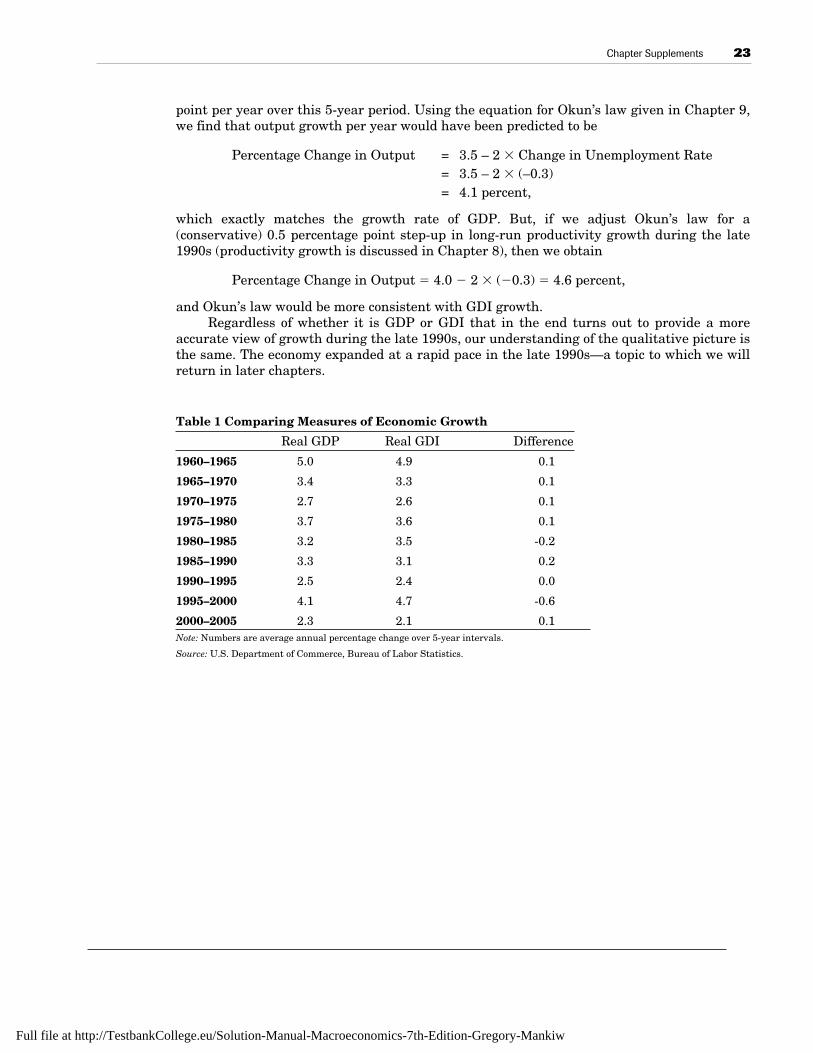
During the late 1990s, however, the statistical discrepancy became unusuallypersistent, even after revisions to historical data. Over the period 1995–2000, the economygrew 4.7 percent per year when measured using real GDI compared with 4.1 percent peryear when measured using real GDP. Table 1 shows annual average growth rates over 5-year periods since 1960. As the table illustrates, the difference in growth rates from the twomeasures has averaged close to zero in the past.
Which Measure Is More Accurate for the Late 1990s?Both the spending and income sides of the national accounts are measured with errorbecause significant portions of the data are estimates based on extrapolations from otherindicators and trends.1 As more complete data become available, the Bureau of EconomicAnalysis revises its estimates of GDP and GDI. Generally, these annual and multiyearrevisions replace more of the spending-side estimates with detailed source data than theincome-side estimates, which often continue to be based on incomplete data. When taxreturns and census data become available, usually with a lag of many years, incomeestimates would be expected to improve. But because these data for income remain far fromcomplete, GDP would still be the more accurate measure, although the discrepancy betweenthe two probably would shrink. The persistence of the difference for the late 1990s, despiteseveral major revisions, has continued to be puzzling.
Another way of gauging the accuracy of GDP compared with GDI is to consider whichmeasure fits better with well-known economic relationships that have typically held in thepast. One such relationship is Okun’s law, a rule of thumb discussed in Chapter 9 thatrelates the growth rate of output to the change in the unemployment rate.2 In particular,Okun’s Law states that a rise in the unemployment rate of 1 percentage point sustained for ayear is associated with a decline in economic growth below its long-run potential rate byabout 2 percentage points. The opposite holds for a fall in the unemployment rate, which isassociated with a rise in economic growth above potential.
Over the period from 1995 to 2000, the unemployment rate declined by 1.6 percentagepoints, from 5.6 percent to 4.0 percent. The decline on average was about 0.3 percentage
1For additional discussion, see The Economic Report of the President, 1997, U.S. Government Printing Office, Washington, pp. 72–74. The Reportargues that from its vantage point back in 1997, Okun’s law seemed to fit better using GDI growth rather than GDP growth. Subsequent revisionsand more data seem to have reversed this finding, as documented below.
2Arthur M. Okun, “Potential GNP: Its Measurement and Significance,” in Proceedings of the Business and Economics Statistics Section, AmericanStatistical Association (Washington, DC: American Statistical Association, 1962), pp. 98–103; reprinted in Arthur M. Okun, Economics forPolicymaking (Cambridge, MA: MIT Press, 1983), pp. 145–158.
Full file at http://TestbankCollege.eu/Solution-Manual-Macroeconomics-7th-Edition-Gregory-Mankiw
Chapter Supplements 23
point per year over this 5-year period. Using the equation for Okun’s law given in Chapter 9,we find that output growth per year would have been predicted to be
Percentage Change in Output = 3.5 – 2 � Change in Unemployment Rate= 3.5 – 2 � (–0.3)= 4.1 percent,
which exactly matches the growth rate of GDP. But, if we adjust Okun’s law for a(conservative) 0.5 percentage point step-up in long-run productivity growth during the late1990s (productivity growth is discussed in Chapter 8), then we obtain
Percentage Change in Output � 4.0 � 2 � (�0.3) � 4.6 percent,
and Okun’s law would be more consistent with GDI growth.Regardless of whether it is GDP or GDI that in the end turns out to provide a more
accurate view of growth during the late 1990s, our understanding of the qualitative picture isthe same. The economy expanded at a rapid pace in the late 1990s—a topic to which we willreturn in later chapters.
Table 1 Comparing Measures of Economic Growth
Real GDP Real GDI Difference
1960–1965 5.0 4.9 0.1
1965–1970 3.4 3.3 0.1
1970–1975 2.7 2.6 0.1
1975–1980 3.7 3.6 0.1
1980–1985 3.2 3.5 -0.2
1985–1990 3.3 3.1 0.2
1990–1995 2.5 2.4 0.0
1995–2000 4.1 4.7 -0.6
2000–2005 2.3 2.1 0.1Note: Numbers are average annual percentage change over 5-year intervals.
Source: U.S. Department of Commerce, Bureau of Labor Statistics.
Full file at http://TestbankCollege.eu/Solution-Manual-Macroeconomics-7th-Edition-Gregory-Mankiw

L E C T U R E S U P P L E M E N T
2-2 Pitfalls in National Income Accounting
Source: Cincinnati magazine.
24
Full file at http://TestbankCollege.eu/Solution-Manual-Macroeconomics-7th-Edition-Gregory-Mankiw
L E C T U R E S U P P L E M E N T
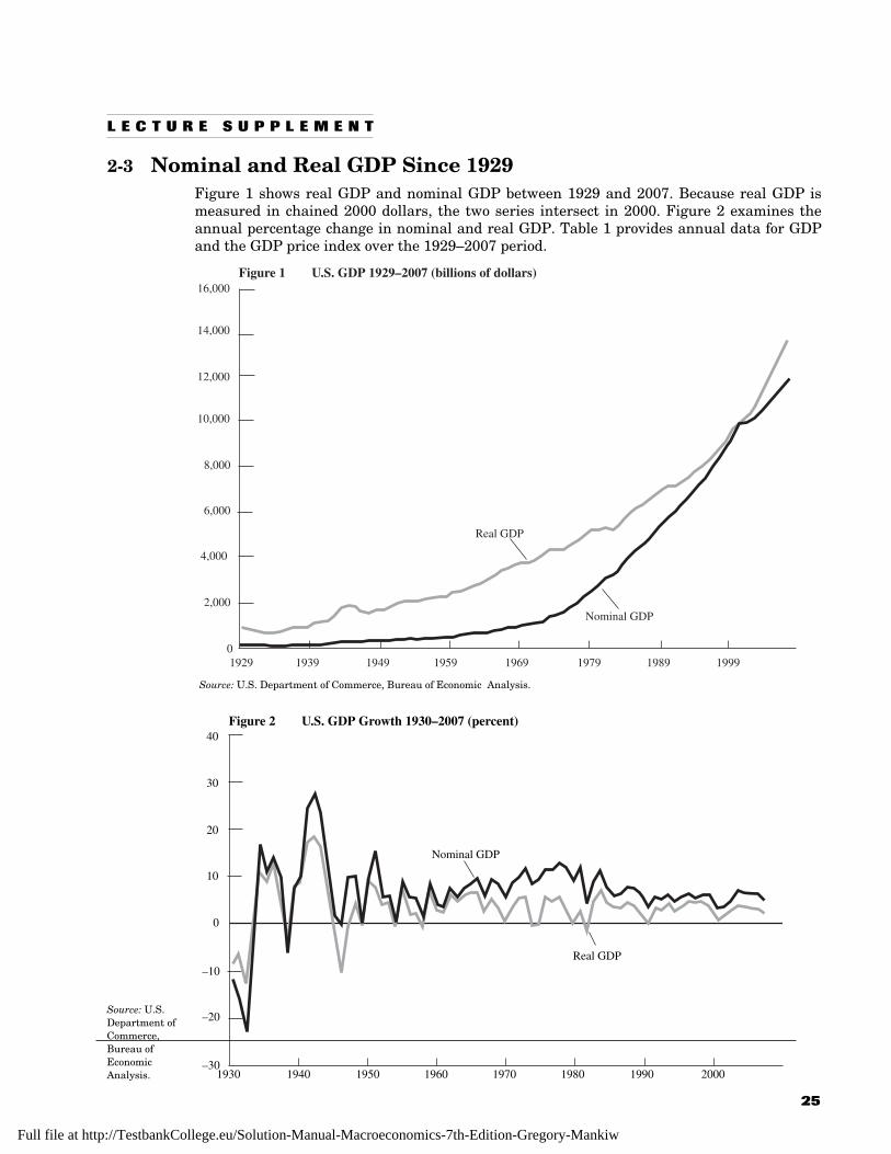
2-3 Nominal and Real GDP Since 1929Figure 1 shows real GDP and nominal GDP between 1929 and 2007. Because real GDP ismeasured in chained 2000 dollars, the two series intersect in 2000. Figure 2 examines theannual percentage change in nominal and real GDP. Table 1 provides annual data for GDPand the GDP price index over the 1929–2007 period.
25
Figure 1 U.S. GDP 1929–2007 (billions of dollars)
12,000
10,000
8,000
16,000
14,000
6,000
4,000
2,000
01929 1939 1949 1959 1969 1979 1999
Real GDP
Nominal GDP
1989
Source: U.S. Department of Commerce, Bureau of Economic Analysis.
–30
–20
10
20
30
40
0
–10
Figure 2 U.S. GDP Growth 1930–2007 (percent)
1930
Real GDP
Nominal GDP
1940 1950 1960 1970 1980 1990 2000
Source: U.S.Department ofCommerce,Bureau ofEconomicAnalysis.
Full file at http://TestbankCollege.eu/Solution-Manual-Macroeconomics-7th-Edition-Gregory-Mankiw

Table 1 United States GDP: 1929–2007
Levels Growth RatesNominal
GDP Real GDP(billions of (billions of GDP Chain-type Nominal GDP Chain-type
current chained 2000 Price Index GDP Real GDP Price IndexYear dollars) dollars) (2000 = 100) (percent) (percent) (percent)
1929 103.6 865.2 11.91930 91.2 790.7 11.5 –12.0 –8.6 –3.91931 76.5 739.9 10.3 –16.1 –6.4 –10.01932 58.7 643.7 9.2 –23.3 –13.0 –11.51933 56.4 635.5 8.9 –3.9 –1.3 –2.61934 66.0 704.2 9.4 17.0 10.8 4.91935 73.3 766.9 9.5 11.1 8.9 2.01936 83.8 866.6 9.6 14.3 13.0 1.21937 91.9 911.1 10.0 9.7 5.1 3.71938 86.1 879.7 9.8 –6.3 –3.4 –1.91939 92.2 950.7 9.7 7.1 8.1 –1.21940 101.4 1034.1 9.8 10.0 8.8 0.91941 126.7 1211.1 10.4 25.0 17.1 6.51942 161.9 1435.4 11.3 27.8 18.5 8.21943 198.6 1670.9 11.9 22.7 16.4 5.61944 219.8 1806.5 12.2 10.7 8.1 2.41945 223.1 1786.3 12.5 1.5 –1.1 2.61946 222.3 1589.4 13.9 –0.4 –11.0 11.71947 244.2 1574.5 15.5 9.9 –0.9 11.21948 269.2 1643.2 16.4 10.2 4.4 5.71949 267.3 1634.6 16.4 –0.7 –0.5 0.01950 293.8 1777.3 16.5 9.9 8.7 0.81951 339.3 1915.0 17.6 15.5 7.7 6.91952 358.3 1988.3 18.0 5.6 3.8 2.21953 379.4 2079.5 18.2 5.9 4.6 1.31954 380.4 2065.4 18.4 0.3 –0.7 1.11955 414.8 2212.8 18.7 9.0 7.1 1.51956 437.5 2255.8 19.4 5.5 1.9 3.51957 461.1 2301.1 20.0 5.4 2.0 3.51958 467.2 2279.2 20.5 1.3 –1.0 2.41959 506.6 2441.3 20.8 8.4 7.1 1.21960 526.4 2501.8 21.0 3.9 2.5 1.41961 544.7 2560.0 21.3 3.5 2.3 1.11962 585.6 2715.2 21.6 7.5 6.1 1.41963 617.7 2834.0 21.8 5.5 4.4 1.11964 663.6 2998.6 22.1 7.4 5.8 1.51965 719.1 3191.1 22.5 8.4 6.4 1.81966 787.8 3399.1 23.2 9.6 6.5 2.81967 832.6 3484.6 23.9 5.7 2.5 3.11968 910.0 3652.7 24.9 9.3 4.8 4.31969 984.6 3765.4 26.2 8.2 3.1 5.01970 1038.5 3771.9 27.5 5.5 0.2 5.31971 1127.1 3898.6 28.9 8.5 3.4 5.01972 1238.3 4105.0 30.2 9.9 5.3 4.31973 1382.7 4341.5 31.9 11.7 5.8 5.6
26 CHAPTER 2 The Data of Macroeconomics
Full file at http://TestbankCollege.eu/Solution-Manual-Macroeconomics-7th-Edition-Gregory-Mankiw
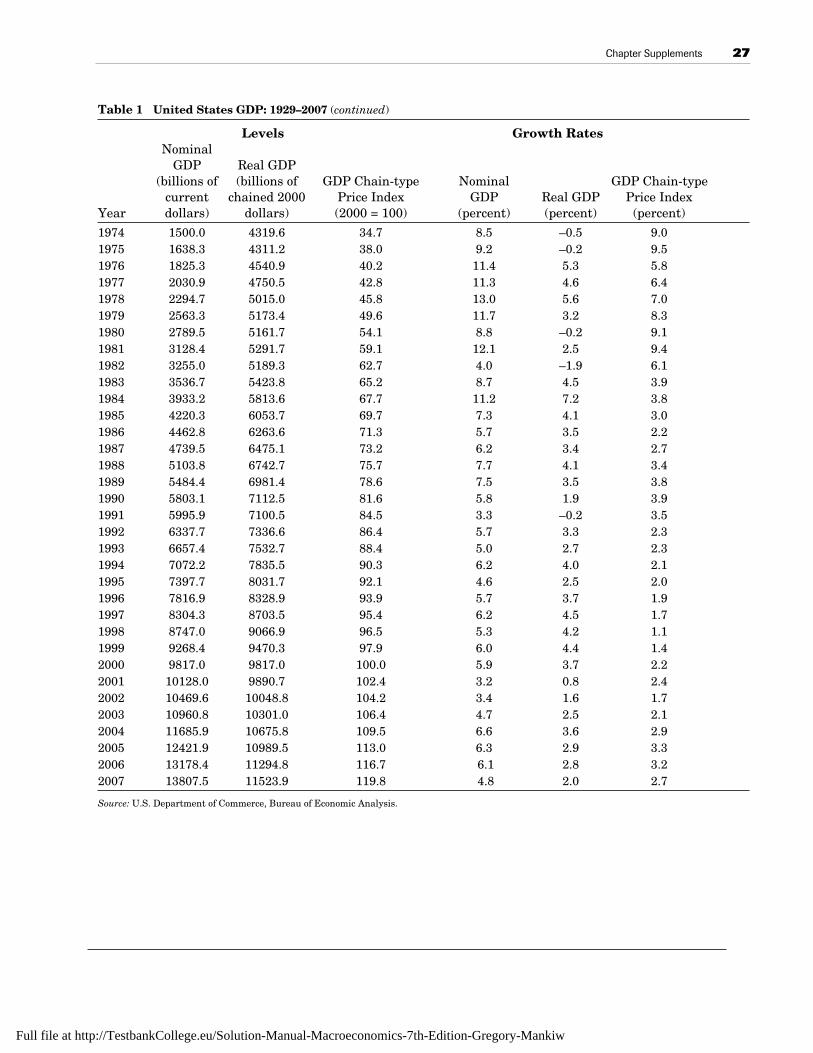
Table 1 United States GDP: 1929–2007 (continued)
Levels Growth RatesNominal
GDP Real GDP(billions of (billions of GDP Chain-type Nominal GDP Chain-type
current chained 2000 Price Index GDP Real GDP Price IndexYear dollars) dollars) (2000 = 100) (percent) (percent) (percent)
1974 1500.0 4319.6 34.7 8.5 –0.5 9.01975 1638.3 4311.2 38.0 9.2 –0.2 9.51976 1825.3 4540.9 40.2 11.4 5.3 5.81977 2030.9 4750.5 42.8 11.3 4.6 6.41978 2294.7 5015.0 45.8 13.0 5.6 7.01979 2563.3 5173.4 49.6 11.7 3.2 8.31980 2789.5 5161.7 54.1 8.8 –0.2 9.11981 3128.4 5291.7 59.1 12.1 2.5 9.41982 3255.0 5189.3 62.7 4.0 –1.9 6.11983 3536.7 5423.8 65.2 8.7 4.5 3.91984 3933.2 5813.6 67.7 11.2 7.2 3.81985 4220.3 6053.7 69.7 7.3 4.1 3.01986 4462.8 6263.6 71.3 5.7 3.5 2.21987 4739.5 6475.1 73.2 6.2 3.4 2.71988 5103.8 6742.7 75.7 7.7 4.1 3.41989 5484.4 6981.4 78.6 7.5 3.5 3.81990 5803.1 7112.5 81.6 5.8 1.9 3.91991 5995.9 7100.5 84.5 3.3 –0.2 3.51992 6337.7 7336.6 86.4 5.7 3.3 2.31993 6657.4 7532.7 88.4 5.0 2.7 2.31994 7072.2 7835.5 90.3 6.2 4.0 2.11995 7397.7 8031.7 92.1 4.6 2.5 2.01996 7816.9 8328.9 93.9 5.7 3.7 1.91997 8304.3 8703.5 95.4 6.2 4.5 1.71998 8747.0 9066.9 96.5 5.3 4.2 1.11999 9268.4 9470.3 97.9 6.0 4.4 1.42000 9817.0 9817.0 100.0 5.9 3.7 2.22001 10128.0 9890.7 102.4 3.2 0.8 2.42002 10469.6 10048.8 104.2 3.4 1.6 1.72003 10960.8 10301.0 106.4 4.7 2.5 2.12004 11685.9 10675.8 109.5 6.6 3.6 2.92005 12421.9 10989.5 113.0 6.3 2.9 3.32006 13178.4 11294.8 116.7 6.1 2.8 3.22007 13807.5 11523.9 119.8 4.8 2.0 2.7
Source: U.S. Department of Commerce, Bureau of Economic Analysis.
Chapter Supplements 27
Full file at http://TestbankCollege.eu/Solution-Manual-Macroeconomics-7th-Edition-Gregory-Mankiw
L E C T U R E S U P P L E M E N T
2-4 Chain-Weight Real GDPFor nearly 50 years, the U.S. Bureau of Economic Analysis calculated real GDP and hencethe growth rate of the economy by valuing goods and services at the prices prevailing in afixed year, known as the base year. Most recently, 1987 was used as the base year. Thus,real GDP in 1995 was calculated by valuing all goods and services produced in 1995 at theprices they sold for in 1987. Similarly, real GDP in 1950 was calculated by valuing all goodsand services produced in 1950 using the prices they sold for in 1987. This method ofcalculating real GDP is known as a fixed-weight measure.
Two major problems are associated with fixed-weight measures of real GDP. First,economic growth may be mismeasured due to substitution bias. Second, attempts to reducethis bias for recent years by periodically updating the base year lead to revisions of historicalgrowth rates.
Substitution bias occurs because goods and services for which output grows rapidly alsotend to be those with prices rising at a less than average rate or possibly declining. As aresult, the farther in time we move away from the base year, the greater, in general, is thedifference between the fixed-price weights of the base year and the actual transaction pricesof goods and services in the economy. Those goods and services experiencing rapid outputgrowth and slowly rising (or declining) prices will tend to receive relatively more weightthan is reflected in current prices and those goods and services experiencing slow outputgrowth and rapidly rising prices will tend to receive relatively less weight. Overall, thisleads to an upward bias in the rate of GDP growth that becomes progressively worse overtime. Likewise, moving back in time over years prior to the base year, GDP growth isunderstated because those goods and services with rapid output growth and slowly growing(or declining prices) are underweighted compared to current prices and those goods andservices with slow output growth and rapidly rising prices are overweighted.
The most widely cited example of substitution bias is computers. The price ofcomputers (holding quality fixed) has declined rapidly and the quantity produced has risensharply. For example, the Bureau of Economic Analysis estimates that the price of a smallmainframe computer was $800,000 in 1977. The same computer cost $80,000 in 1987 and$30,000 in 1995.1 If each computer sold in 1995 was valued at its 1987 price, real GDP wouldbe biased upward. Likewise, if each computer sold in 1977 was valued at its 1987 price, realGDP in 1977 would be biased downward.
Substitution bias not only produces a mismeasurement of real output, but it also canresult in a mismeasurement of the relative importance of the components of output: consump-tion, investment, government expenditures, and net exports. Computers are primarilycounted as an investment good in the national accounts. Thus, the rapid increase in the out-put of computers over the past two decades would lead to an overstatement of the contri-bution of investment to GDP growth in the years after the base year and an understatementof the contribution of investment to growth in the years prior to the base year.
To reduce the extent of mismeasurement for recent years, the base year was updatedevery 5 years. In 1991 the base year was changed from 1982 to 1987. Changing the baseyear, however, affects the measurement of economic growth in all years. While moving thebase year forward provides a more accurate measurement of current growth, it worsens theunderestimation of growth in early years.
28
1J. Steven Landefeld and Robert P. Parker, “Preview of the Comprehensive Revision of the National Income and Product Accounts: BEA’s NewFeatured Measures of Output and Prices,” Survey of Current Business, July 1995.
Full file at http://TestbankCollege.eu/Solution-Manual-Macroeconomics-7th-Edition-Gregory-Mankiw
In 1996, rather than updating the base year to 1992, the Bureau of Economic Analysisswitched the method it used to calculate economic growth because of the substitution biasand rewriting of history that occurred with a fixed-weight measure. Real GDP growth in anyyear, t, is now calculated using prices from year t and t – 1. This method minimizes thesubstitution bias because recent prices are used and eliminates the historical revisions thatoccurred when the base year was updated.2
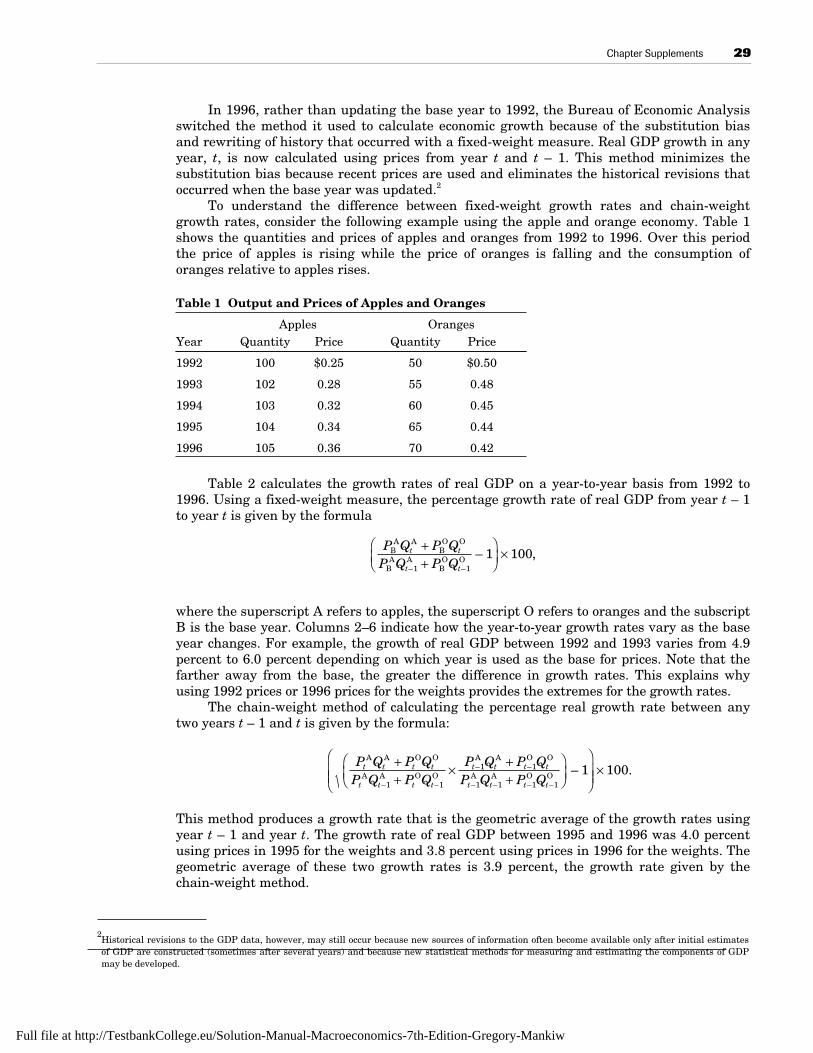
To understand the difference between fixed-weight growth rates and chain-weightgrowth rates, consider the following example using the apple and orange economy. Table 1shows the quantities and prices of apples and oranges from 1992 to 1996. Over this periodthe price of apples is rising while the price of oranges is falling and the consumption oforanges relative to apples rises.
Table 1 Output and Prices of Apples and Oranges
Apples OrangesYear Quantity Price Quantity Price
1992 100 $0.25 50 $0.50
1993 102 0.28 55 0.48
1994 103 0.32 60 0.45
1995 104 0.34 65 0.44
1996 105 0.36 70 0.42
Table 2 calculates the growth rates of real GDP on a year-to-year basis from 1992 to1996. Using a fixed-weight measure, the percentage growth rate of real GDP from year t – 1to year t is given by the formula
where the superscript A refers to apples, the superscript O refers to oranges and the subscriptB is the base year. Columns 2–6 indicate how the year-to-year growth rates vary as the baseyear changes. For example, the growth of real GDP between 1992 and 1993 varies from 4.9percent to 6.0 percent depending on which year is used as the base for prices. Note that thefarther away from the base, the greater the difference in growth rates. This explains whyusing 1992 prices or 1996 prices for the weights provides the extremes for the growth rates.
The chain-weight method of calculating the percentage real growth rate between anytwo years t – 1 and t is given by the formula:
This method produces a growth rate that is the geometric average of the growth rates usingyear t – 1 and year t. The growth rate of real GDP between 1995 and 1996 was 4.0 percentusing prices in 1995 for the weights and 3.8 percent using prices in 1996 for the weights. Thegeometric average of these two growth rates is 3.9 percent, the growth rate given by thechain-weight method.
Chapter Supplements 29
P Q P QP Q P Q
t t
t t
BA A
B
BA
–A
B –
– ,++
⎛⎝⎜
⎞⎠⎟
×O O
O O1 1
1 100
P Q P QP Q P Q
P Q P QP Q P Q
t t t t
t t t t
t t t t
t t t t
A A
A–A
–
–A A
–
–A
–A
– –
– .++
× ++
⎛⎝⎜
⎞⎠⎟
⎛
⎝⎜⎜
⎞
⎠⎟⎟ ×
O O
O O
O O
O O1 1
1 1
1 1 1 1
1 100
2Historical revisions to the GDP data, however, may still occur because new sources of information often become available only after initial estimatesof GDP are constructed (sometimes after several years) and because new statistical methods for measuring and estimating the components of GDPmay be developed.
Full file at http://TestbankCollege.eu/Solution-Manual-Macroeconomics-7th-Edition-Gregory-Mankiw
30 CHAPTER 2 The Data of Macroeconomics
Table 2 Growth Rate of Real Output Using Fixed-Weight or Chain-Weight Method
1992 1993 1994 1995 1996 Chain-Base Base Base Base Base Weight
1992–93 6.0% 5.7% 5.3% 5.1% 4.9% 5.8%
1993–94 5.2 4.9 4.5 4.3 4.1 4.7
1994–95 4.9 4.6 4.3 4.1 3.9 4.2
1995–96 4.7 4.4 4.1 4.0 3.8 3.9
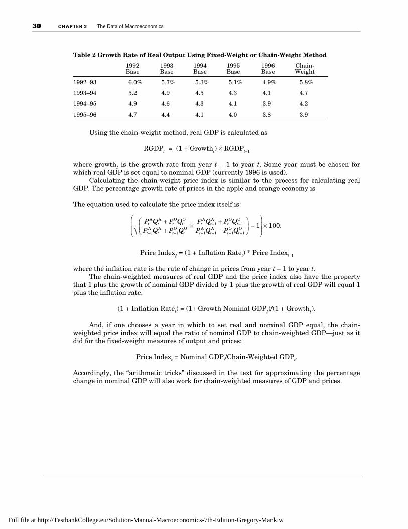
Using the chain-weight method, real GDP is calculated as
RGDPt = (1 + Growtht) × RGDPt–1
where growtht is the growth rate from year t – 1 to year t. Some year must be chosen forwhich real GDP is set equal to nominal GDP (currently 1996 is used).
Calculating the chain-weight price index is similar to the process for calculating realGDP. The percentage growth rate of prices in the apple and orange economy is
The equation used to calculate the price index itself is:
Price Indext = (1 + Inflation Ratet) * Price Indext–1
where the inflation rate is the rate of change in prices from year t – 1 to year t.The chain-weighted measures of real GDP and the price index also have the property
that 1 plus the growth of nominal GDP divided by 1 plus the growth of real GDP will equal 1plus the inflation rate:
(1 + Inflation Ratet) = (1+ Growth Nominal GDPt)/(1 + Growtht).
And, if one chooses a year in which to set real and nominal GDP equal, the chain-weighted price index will equal the ratio of nominal GDP to chain-weighted GDP—just as itdid for the fixed-weight measures of output and prices:
Price Indext = Nominal GDPt/Chain-Weighted GDPt.
Accordingly, the “arithmetic tricks” discussed in the text for approximating the percentagechange in nominal GDP will also work for chain-weighted measures of GDP and prices.
P Q P QP Q P Q
P Q P QP Q P Q
t t t t
t t t t
t t t t
t t t t
A A
–A A
–
A–A
–
–A
–A
– –
– .++
× ++
⎛⎝⎜
⎞⎠⎟
⎛
⎝⎜⎜
⎞
⎠⎟⎟ ×
O O
O O
O O
O O1 1
1 1
1 1 1 1
1 100
Full file at http://TestbankCollege.eu/Solution-Manual-Macroeconomics-7th-Edition-Gregory-Mankiw

Chapter Supplements 31
A D D I T I O N A L C A S E S T U D Y
2-5 The Increasing Role of ServicesIn the United States and in other developed countries, an increasing fraction of output isaccounted for by services. The following article, from The Economist, February 20, 1993,details this phenomenon.
The Final Frontier
The industrial economies should be renamedthe service economies: they employ twice asmany workers in services as in industry
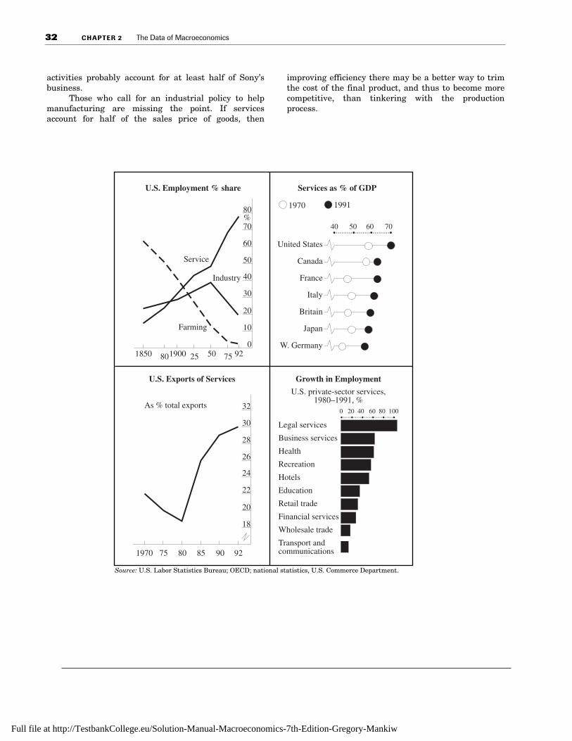
The growth of services is nothing new. As early as1900, America and Britain both had more jobs inservices than in industry. By 1950 services employedhalf of all American workers. Last year the figure hit76%.
America has by far the biggest service sector,accounting for 72% of its GDP. At the rich world’s otherextreme, Germany’s still provides only 57% of its GDP,thanks partly to a multitude of restrictive practiceswhich have choked expansion.
Meanwhile, the share of manufacturing hasfallen in all the big economies. It now accounts for only23% of America’s GDP (and an even smaller 18% ofjobs). In Britain and Canada manufacturing hastumbled to less than 20% of total output. Even inJapan and Germany, the strongholds of industry,manufacturing is now no more than 30% of GDP.
Services are also the fastest-growing part ofinternational trade, accounting for 20% of total worldtrade and 30% of American exports. This excludesthose services that are not traded, but are delivered bysubsidiaries set up in foreign markets. Services accountfor about 40% of the stock of foreign direct investmentby the five big “industrial economies.”
Sales of services by the foreign affiliates ofAmerican companies were worth $119 billion in 1990(the latest figures available), not far behind America’s$138 billion-worth of cross-border sales of privateservices. These sales do not contribute directly tooutput or jobs in America, but the economy does benefitwhen the profits from American company operationsabroad are brought home. As governments open theirborders to foreign companies, the scope for futureexpansion of trade and foreign direct investment inservices is huge.
Policemen and prostitutes, bankers and butchersare all lumped together in the service sector, but not allhave grown at the same rate. The chart on the [bottom]right [on the next page] compares the growth in jobs insome selected American service industries since 1980.Top of the league are legal and business services, whichgrew by 106% and 67%, respectively, followed closely
by health (59%) and recreation (53%). Jobs in olderservices grew more slowly. Employment in transportand communication, for instance, grew by only 13%.
Some economists argue that the boom in servicesis caused mainly by firms contracting out jobs theyused to do for themselves, such as catering, advertisingand data-processing. But studies in America andBritain suggest that this explains only a fraction of theincrease.
If anything, official figures may understate thetrue importance of services in both output and jobs, asmany activities in manufacturing firms are reallyservices. Government number-crunchers stick TheEconomist, along with all newspapers, in the manufac-turing sector, even though few employees actuallymake anything. The work of a freelance journalist, bycontrast, is counted in the service sector. The divisionbetween services and manufacturing is becomingsteadily less useful.
As a recent OEC report1 points out, services andmanufacturing have become increasingly intercon-nected, as manufacturers buy more inputs from servicefirms and vice versa. Higher spending on advertising,financial management, and a speedier delivery systemmean that more service value is added to each unit ofmanufacturing output.
Take General Motors, the archetypal manufac-turer. Its biggest single supplier is not a steel or glassfirm, but a health-care provider, Blue Cross-BlueShield. In terms of output, one of GM’s biggest “prod-ucts” is financial and insurance services, which to-gether with EDS, its computing-services arm, accountfor a fifth of total revenue.
But few manufacturers will admit how much theyrely on services. Sony’s chairman, Akio Morita, pro-claimed in a speech at this year’s meeting of the WorldEconomic Forum in Davos that “an increased focus onmanufacturing will help us to re-lay the foundation ofour economy. Only manufacturing can provide employ-ment opportunities of quality, scope and number. . . .The service sector can only survive if there is a pro-ductive manufacturing sector to serve.” Yet look closerat Sony: as much as a fifth of its revenues now comefrom its film and music businesses. Add in design,marketing, finance, and after-sales support, and service
1“Structural Shifts in Major OECD Countries,” in “Industrial Policy in
OECD Countries: Annual Review, 1992.” Published by the OECD.
Full file at http://TestbankCollege.eu/Solution-Manual-Macroeconomics-7th-Edition-Gregory-Mankiw
32 CHAPTER 2 The Data of Macroeconomics
United States
Canada
France
Italy
Britain
Japan
W. Germany
40 50 60 70•.........•........•.........•
1970 1991
Services as % of GDP
90 92
18
20
22
24
26
28
30
32
U.S. Exports of Services
1970 75 80 85
As % total exports
1850 801900 25 50 75 920
10
20
30
40
50
60
70
80%
Service
Industry
Farming
U.S. Employment % share
Growth in Employment
U.S. private-sector services, 1980–1991, %
Legal services
Business services
Health
Recreation
Hotels
Education
Retail trade
Financial services
Wholesale trade
Transport andcommunications
0 20 40 60 80 100•.....•.....•.....•.....•.....•
Source: U.S. Labor Statistics Bureau; OECD; national statistics, U.S. Commerce Department.
activities probably account for at least half of Sony’sbusiness.
Those who call for an industrial policy to helpmanufacturing are missing the point. If servicesaccount for half of the sales price of goods, then
improving efficiency there may be a better way to trimthe cost of the final product, and thus to become morecompetitive, than tinkering with the productionprocess.
Full file at http://TestbankCollege.eu/Solution-Manual-Macroeconomics-7th-Edition-Gregory-Mankiw

33
C A S E S T U D Y E X T E N S I O N p. 28
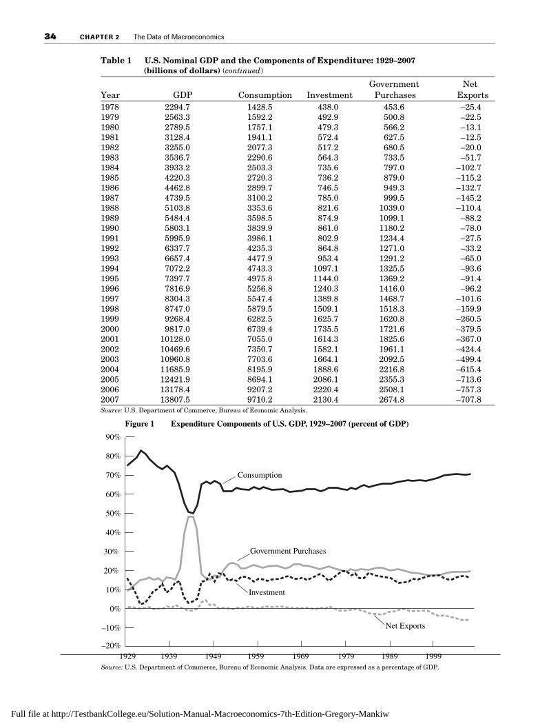
2-6 The Components of GDPTable 1 and Figure 1 show the principal components of GDP between 1929 and 2007.
Table 1 U.S. Nominal GDP and the Components of Expenditure: 1929–2007(billions of dollars)
Government NetYear GDP Consumption Investment Purchases Exports 1929 103.6 77.4 16.5 9.4 0.41930 91.2 70.1 10.8 10.0 0.31931 76.5 60.7 5.9 9.9 0.01932 58.7 48.7 1.3 8.7 0.01933 56.4 45.9 1.7 8.7 0.11934 66.0 51.5 3.7 10.5 0.31935 73.3 55.9 6.7 10.9 –0.21936 83.8 62.2 8.6 13.1 –0.11937 91.9 66.8 12.2 12.8 0.11938 86.1 64.3 7.1 13.8 1.01939 92.2 67.2 9.3 14.8 0.81940 101.4 71.3 13.6 15.0 1.51941 126.7 81.1 18.1 26.5 1.01942 161.9 89.0 10.4 62.7 –0.31943 198.6 99.9 6.1 94.8 –2.21944 219.8 108.7 7.8 105.3 –2.01945 223.1 120.0 10.8 93.0 –0.81946 222.3 144.3 31.1 39.6 7.21947 244.2 162.0 35.0 36.4 10.81948 269.2 175.0 48.1 40.6 5.51949 267.3 178.5 36.9 46.7 5.21950 293.8 192.2 54.1 46.8 0.71951 339.3 208.5 60.2 68.1 2.51952 358.3 219.5 54.0 83.6 1.21953 379.4 233.1 56.4 90.6 –0.71954 380.4 240.0 53.8 86.2 0.41955 414.8 258.8 69.0 86.5 0.51956 437.5 271.7 72.0 91.4 2.41957 461.1 286.9 70.5 99.7 4.11958 467.2 296.2 64.5 106.0 0.51959 506.6 317.6 78.5 110.0 0.41960 526.4 331.7 78.9 111.6 4.21961 544.7 342.1 78.2 119.5 4.91962 585.6 363.3 88.1 130.1 4.11963 617.7 382.7 93.8 136.4 4.91964 663.6 411.4 102.1 143.2 6.91965 719.1 443.8 118.2 151.5 5.61966 787.8 480.9 131.3 171.8 3.91967 832.6 507.8 128.6 192.7 3.61968 910.0 558.0 141.2 209.4 1.41969 984.6 605.2 156.4 221.5 1.41970 1038.5 648.5 152.4 233.8 4.01971 1127.1 701.9 178.2 246.5 0.61972 1238.3 770.6 207.6 263.5 –3.41973 1382.7 852.4 244.5 281.7 4.11974 1500.0 933.4 249.4 317.9 –0.81975 1638.3 1034.4 230.2 357.7 16.01976 1825.3 1151.9 292.0 383.0 –1.61977 2030.9 1278.6 361.3 414.1 –23.1
Full file at http://TestbankCollege.eu/Solution-Manual-Macroeconomics-7th-Edition-Gregory-Mankiw
34 CHAPTER 2 The Data of Macroeconomics
Table 1 U.S. Nominal GDP and the Components of Expenditure: 1929–2007(billions of dollars) (continued)
Government NetYear GDP Consumption Investment Purchases Exports 1978 2294.7 1428.5 438.0 453.6 –25.41979 2563.3 1592.2 492.9 500.8 –22.51980 2789.5 1757.1 479.3 566.2 –13.11981 3128.4 1941.1 572.4 627.5 –12.51982 3255.0 2077.3 517.2 680.5 –20.01983 3536.7 2290.6 564.3 733.5 –51.71984 3933.2 2503.3 735.6 797.0 –102.71985 4220.3 2720.3 736.2 879.0 –115.21986 4462.8 2899.7 746.5 949.3 –132.71987 4739.5 3100.2 785.0 999.5 –145.21988 5103.8 3353.6 821.6 1039.0 –110.41989 5484.4 3598.5 874.9 1099.1 –88.21990 5803.1 3839.9 861.0 1180.2 –78.01991 5995.9 3986.1 802.9 1234.4 –27.51992 6337.7 4235.3 864.8 1271.0 –33.21993 6657.4 4477.9 953.4 1291.2 –65.01994 7072.2 4743.3 1097.1 1325.5 –93.61995 7397.7 4975.8 1144.0 1369.2 –91.41996 7816.9 5256.8 1240.3 1416.0 –96.21997 8304.3 5547.4 1389.8 1468.7 –101.61998 8747.0 5879.5 1509.1 1518.3 –159.91999 9268.4 6282.5 1625.7 1620.8 –260.52000 9817.0 6739.4 1735.5 1721.6 –379.52001 10128.0 7055.0 1614.3 1825.6 –367.02002 10469.6 7350.7 1582.1 1961.1 –424.42003 10960.8 7703.6 1664.1 2092.5 –499.42004 11685.9 8195.9 1888.6 2216.8 –615.42005 12421.9 8694.1 2086.1 2355.3 –713.62006 13178.4 9207.2 2220.4 2508.1 –757.32007 13807.5 9710.2 2130.4 2674.8 –707.8Source: U.S. Department of Commerce, Bureau of Economic Analysis.
Figure 1 Expenditure Components of U.S. GDP, 1929–2007 (percent of GDP)
90%
80%
60%
70%
40%
50%
20%
30%
0%
10%
–10%
–20%1929 1939 1949 1959 1969 1979 1999
Consumption
Government Purchases
Investment
Net Exports
1989Source: U.S. Department of Commerce, Bureau of Economic Analysis. Data are expressed as a percentage of GDP.
Full file at http://TestbankCollege.eu/Solution-Manual-Macroeconomics-7th-Edition-Gregory-Mankiw
As Figure 1 illustrates, the GDP shares of consumption expenditure, private investmentexpenditure, and government purchases have been relatively constant over the past 50years. Earlier in the twentieth century, however, the story was much different asexpenditure shares shifted sharply. During the Great Depression of the early 1930s, thecollapse of investment spending led to a decline in its share of GDP while the share ofconsumption expenditure increased. During World War II, the Federal government’sexpansion pushed government purchases to nearly 50 percent of GDP, while the shares ofprivate investment and consumption plummeted.
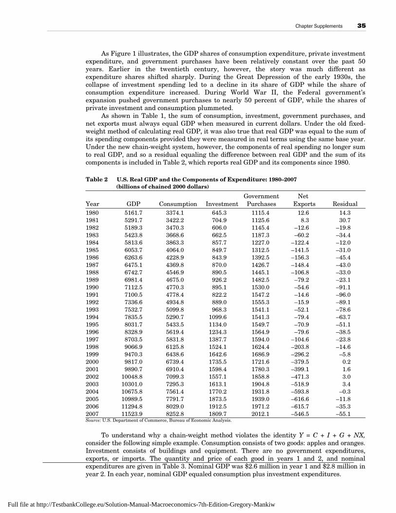
As shown in Table 1, the sum of consumption, investment, government purchases, andnet exports must always equal GDP when measured in current dollars. Under the old fixed-weight method of calculating real GDP, it was also true that real GDP was equal to the sum ofits spending components provided they were measured in real terms using the same base year.Under the new chain-weight system, however, the components of real spending no longer sumto real GDP, and so a residual equaling the difference between real GDP and the sum of itscomponents is included in Table 2, which reports real GDP and its components since 1980.
Table 2 U.S. Real GDP and the Components of Expenditure: 1980–2007(billions of chained 2000 dollars)
Government NetYear GDP Consumption Investment Purchases Exports Residual1980 5161.7 3374.1 645.3 1115.4 12.6 14.31981 5291.7 3422.2 704.9 1125.6 8.3 30.71982 5189.3 3470.3 606.0 1145.4 –12.6 –19.81983 5423.8 3668.6 662.5 1187.3 –60.2 –34.41984 5813.6 3863.3 857.7 1227.0 –122.4 –12.01985 6053.7 4064.0 849.7 1312.5 –141.5 –31.01986 6263.6 4228.9 843.9 1392.5 –156.3 –45.41987 6475.1 4369.8 870.0 1426.7 –148.4 –43.01988 6742.7 4546.9 890.5 1445.1 –106.8 –33.01989 6981.4 4675.0 926.2 1482.5 –79.2 –23.11990 7112.5 4770.3 895.1 1530.0 –54.6 –91.11991 7100.5 4778.4 822.2 1547.2 –14.6 –96.01992 7336.6 4934.8 889.0 1555.3 –15.9 –89.11993 7532.7 5099.8 968.3 1541.1 –52.1 –78.61994 7835.5 5290.7 1099.6 1541.3 –79.4 –63.71995 8031.7 5433.5 1134.0 1549.7 –70.9 –51.11996 8328.9 5619.4 1234.3 1564.9 –79.6 –38.51997 8703.5 5831.8 1387.7 1594.0 –104.6 –23.81998 9066.9 6125.8 1524.1 1624.4 –203.8 –14.61999 9470.3 6438.6 1642.6 1686.9 –296.2 –5.82000 9817.0 6739.4 1735.5 1721.6 –379.5 0.22001 9890.7 6910.4 1598.4 1780.3 –399.1 1.62002 10048.8 7099.3 1557.1 1858.8 –471.3 3.02003 10301.0 7295.3 1613.1 1904.8 –518.9 3.42004 10675.8 7561.4 1770.2 1931.8 –593.8 –0.32005 10989.5 7791.7 1873.5 1939.0 –616.6 –11.82006 11294.8 8029.0 1912.5 1971.2 –615.7 –35.32007 11523.9 8252.8 1809.7 2012.1 –546.5 –55.1Source: U.S. Department of Commerce, Bureau of Economic Analysis.
To understand why a chain-weight method violates the identity Y = C + I + G + NX,consider the following simple example. Consumption consists of two goods: apples and oranges.Investment consists of buildings and equipment. There are no government expenditures,exports, or imports. The quantity and price of each good in years 1 and 2, and nominalexpenditures are given in Table 3. Nominal GDP was $2.6 million in year 1 and $2.8 million inyear 2. In each year, nominal GDP equaled consumption plus investment expenditures.
Chapter Supplements 35
Full file at http://TestbankCollege.eu/Solution-Manual-Macroeconomics-7th-Edition-Gregory-Mankiw

Calculating real GDP under the fixed-weight method in this economy is easy. Supposeyear 1 is the base year. Then real consumption and investment are $1.5 million and $1.1million, respectively, in year 1, and real GDP is $2.6 million. In year 2, real consumption iscalculated by valuing the quantity of apples and the quantity of oranges at their year 1prices. Thus,
C2 = P Q + P Q
= $1,875,000.
Real investment in year 2 is calculated by valuing the quantity of buildings and the quantityof equipment at their year 1 prices. Thus,
I2 = P Q + P Q
= $875,000.
Real GDP in year 2 is calculated by valuing the quantity of each good produced at its price inyear 1. Thus,
Real GDP2 = P Q + P Q + P Q + P Q
= C2 + I2
= $1,875,000 + $875,000
= $2,750,000.
From the above formula it is clear that the sum of real consumption and real investment willalways equal real GDP.
The chain-weight method of calculating real GDP is not so simple. Real consumption,investment, and GDP in year 1 are set at their nominal values. Real consumption in year 2equals real consumption in year 1 multiplied by the geometric average of the quantity ofapples and oranges in year 2 valued at their year 1 prices divided by the actual expenditureson apples and oranges in year 1, and the actual expenditures on apples and oranges in year2 divided by the quantity of apples and oranges in year 1 valued at their year 2 prices:
C2 =
= 1.2099 × $1,500,000
= $1,814,850.
P Q P Q
P Q P Q
P Q P Q
P Q P QCapples apples oranges oranges
apples apples oranges oranges
apples apples oranges oranges
apples apples oranges oranges
1 2 1 2
1 1 1 1
2 2 2 2
2 1 2 11+
+⎛
⎝⎜⎞
⎠⎟++
⎛
⎝⎜⎞
⎠⎟×
1apples
2apples
1oranges
2oranges
1apples
2apples
1oranges
2oranges
1buildings
2buildings
1equipment
2equipment
1buildings
2buildings
1equipment
2equipment
Table 3 Calculating GDP and Its Components
Year 1 Year 2
Quantity Price Expenditures Quantity Price Expenditures
Apples 4,000,000 $.25 $1,000,000 3,500,000 $.28 $980,000
Oranges 1,000,000 $.5 $500,000 2,000,000 $.4 $800,000
Consumption $1,500,000 $1,780,000
Buildings 5 $200,000 $1,000,000 4 $225,000 $900,000
Equipment 10 $5,000 $50,000 15 $4,750 $71,250
Investment $1,050,000 $971,250
GDP $2,550,000 $2,751,250
36 CHAPTER 2 The Data of Macroeconomics
Full file at http://TestbankCollege.eu/Solution-Manual-Macroeconomics-7th-Edition-Gregory-Mankiw

Similarly, real investment in year 2 is equal to real investment in year 1 multiplied by thegeometric average of the quantity of buildings and investment in year 2 valued at their year1 prices divided by the actual expenditures on buildings and equipment in year 1, and theactual expenditures on building and equipment in year 2 divided by the quantity of buildingsand equipment in year 1 valued at their year 2 prices:
I2 =
= 0.8308 × $1,050,000
= $872,340.
The formula used to calculate real GDP under the chain-weight method is not the sum of theformulas used to calculate the components (as is the case under a fixed-weight calculation).Therefore, the components do not sum to GDP. The formula for real GDP in year 2 is:
GDP2 =
= 1.0498 × $2,550,000
= $2,676,990.
The residual is
GDP2 – (C2 + I2) = $2,676,990 – ($1,814,850 + $872,340)= $2,676,990 – ($2,687,190)= – $10,220.
In Table 2, the residual is larger in earlier years and also exhibits sharper swings betweenyears. Because the residual tends to grow in size and variability as one moves away in timefrom the year in which the nominal and real series are linked, the chained-dollar GDP andits components are not very useful for comparing the relative shares of different realspending components in years distant from the link date. In gauging the comparative size ofspending components, the nominal shares shown in Figure 1 are much more appropriatemeasures.
Chapter Supplements 37
P Q P Q
P Q P Q
P Q P Q
P Q P QIbuildings buildings equipment equipment
buildings buildings equipment equipment
buildings buildings equipment equipment
buildings buildings oranges equipment
1 2 1 2
1 1 1 1
2 2 2 2
2 1 2 11+
+⎛
⎝⎜⎞
⎠⎟++
⎛
⎝⎜⎞
⎠⎟×
P Q P Q P Q P QP Q P Q P Q P Q
P Q P Q P Q P QP Q P Q P Q P Q
a a o o b b e e
a a o o b b e e
a a o o b b e e
a a o o b b e e
1 2 1 2 1 2 1 2
1 1 1 1 1 1 1 1
2 2 2 2 2 2 2 2
2 1 2 1 2 1 2 1
+ + ++ + +
⎛⎝⎜
⎞⎠⎟
+ + ++ + +
⎛⎝⎜
⎞⎞⎠⎟
× GDP1
Full file at http://TestbankCollege.eu/Solution-Manual-Macroeconomics-7th-Edition-Gregory-Mankiw
L E C T U R E S U P P L E M E N T
2-7 Defining National IncomeIn December 2003, the Bureau of Economic Analysis at the U.S. Department of Commercereleased one of its periodic comprehensive revisions of the National Income and ProductAccounts. These revisions employ additional source data, improved estimation methods, andchanges in definitions and classifications. With the December 2003 revision, the Bureauadopted the definition of national income recommended by the System of National Accounts19931, the principal international guidelines for national accounts data.2
Since 1993, the Bureau gradually has adopted most of the major changes recommendedby these international guidelines, including the move in 1996 to chain-weight indexes formeasuring changes in real GDP and prices (see Supplement 2-4). As the Bureau noted inannouncing its 2003 revision, “integration of the world’s monetary, fiscal, and trade policieshas led to a growing need for international harmonization of economic statistics. Many of thedefinitional changes presented in this year’s revision will improve consistency with theprinciple international guidelines for national accounts.” 3
National income was redefined to equal gross national product minus consumption offixed capital. Thus, national income now includes all net incomes, not only factor incomesaccruing to labor and owners of capital. These non-factor charges—primarily indirectbusiness taxes—are now included in the official definition of national income. This change,however, does not affect personal income or saving because these non-factor charges aresubtracted from national income to obtain personal income. As with most definitionalchanges, the Bureau has implemented the new measure of national income back to 1929, somacroeconomists working with historical data will have a consistent data series for theirresearch.
38
1See Commission of the European Communities, International Monetary Fund, Organization for Economic Co-operation and Development, UnitedNations, and the World Bank, System of National Accounts 1993 (Brussels/Luxembourg, New York, Paris, and Washington, DC, 1993).
2See “New International Guidelines in Economic Accounting,” Survey of Current Business 73 (February 1993).
3“Preview of the 2003 Comprehensive Revision of the National Income and Product Accounts,” Survey of Current Business, 83 (June 2003), p. 18.
Full file at http://TestbankCollege.eu/Solution-Manual-Macroeconomics-7th-Edition-Gregory-Mankiw
L E C T U R E S U P P L E M E N T
2-8 Seasonal Adjustment and the Seasonal CycleEconomists use various techniques to describe economic data. One set of techniquesinvolves decomposing data series into constituent subseries that can be added together togive the total series. As an example, economists often separate GDP into a long-run, ortrend, component and a short-run, or business cycle, component.1 Another decompositioninvolves removing the seasonal component from economic data. Sophisticated statisticaltechniques (known as spectral analysis) are used to carry out these decompositions. We canthus take a data series (say, for GDP), detrend it, and then divide it into a seasonal seriesand a seasonally adjusted cyclical series. The overall series for GDP would then be the sumof a long-run trend, a shorter-run cyclical component, and a very short-run seasonalcomponent.2 Most investigations of business cycles carry out just such a decomposition andfocus on the seasonally adjusted cyclical component of different economic data series. Thefact that these data series exhibit certain regularities is the primary motivation for thestudy of business cycles in Part IV of the textbook.
Robert Barsky and Jeffrey Miron decided instead to look at the seasonal component ofthe data.3 Interestingly, they found that the same sort of regularities that are observed inbusiness cycle data also show up in seasonal data. Moreover, they found that seasonalfluctuations are significant in the sense that they account for much of the variation indetrended data. Seasonal fluctuations were found in all major components of GDP.
All major components of GDP with the exception of fixed investment display the sameseasonal pattern: a large decline in the first quarter, small declines in the second and thirdquarters, and a large increase in the fourth quarter. Fixed investment shows declines in thefirst and fourth quarters, and increases in the second and third quarters. An obviousexplanation of seasonal variation is weather but, with the exception of the fixed investmentseries, it is difficult to reconcile seasonal patterns with this explanation. Other key findingsare that, just as in business cycle data, money is procyclical (that is, money and outputmovements are positively correlated), as is labor productivity. Similarly, prices exhibit muchless variation than quantities in seasonal data, as they do in business cycle data. Sales andproduction are also correlated at a seasonal as well as a cyclical level.
Barsky and Miron argue that the similarity of seasonal and business cycles suggeststhat we should look for similar explanations of the two phenomena. Moreover, since many ofthe forces behind seasonal fluctuations can clearly be anticipated (there is a spending shockas a result of Christmas shopping at the same time every year), the distinction betweenanticipated and unanticipated shocks may not be as important for the business cycle as sometheories suggest.4 Whereas seasonal and business cycles may be initially generated bydifferent shocks, they may be driven by similar propagation mechanisms.5
The finding that money is procyclical in seasonal data indicates that the causalrelationship runs from output to money, and not vice versa (since monetary expansionspresumably do not cause Christmas). The view that money may be endogenous at thecyclical level is important to real-business-cycle theory (discussed in Chapter 19 of thetextbook). Finally, the seasonal correlation between production and sales raises questions forthe production-smoothing model of inventories discussed in Chapter 17 of the textbook.6
39
1There are, in turn, a number of different ways to detrend data. See Supplements 9-2, “Understanding Business Cycles I: The Stylized Facts,” and 19-8, “Real Business Cycles and Random Walks” for related discussions.
2In the terminology of spectral analysis, these are referred to as different frequencies. Roughly speaking, short-run fluctuations occur at highfrequencies, and long-run fluctuations at low frequencies.
3R. Barsky and J. Miron, “The Seasonal Cycle and the Business Cycle,” Journal of Political Economy 97 (June 1989): 503–34.
4See, in particular, the models of aggregate supply in Chapter 13 and Supplement 13-2, “Anticipated and Unanticipated Money.”
5See Supplement 9-7, “Understanding Business Cycles II: Modeling Cycles.”
6See Supplement 17-6, “Inventories and Production Smoothing.”
Full file at http://TestbankCollege.eu/Solution-Manual-Macroeconomics-7th-Edition-Gregory-Mankiw
C A S E S T U D Y E X T E N S I O N p. 35
2-9 Measuring the Price of LightAccording to William Nordhaus, unmeasured changes in quality dramatically overestimatethe true rise in the cost of living, as measured by the consumer price index (CPI).1 Nordhaususes a simple example of estimating the price of light to illustrate the importance of qualitychanges and the effect that not accounting for these changes can have on the measurementof inflation. Nordhaus traces the use of artificial light from fire to fat burning lamps tocandles to kerosene lamps to the electric light bulb.
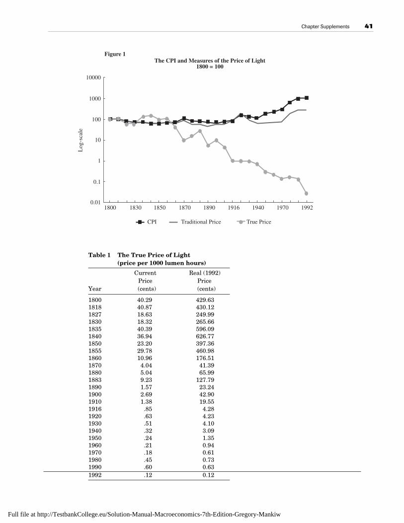
There are two ways to measure the price of light. The first, which Nordhaus refers to asthe traditional way, is to measure the price of the good that provides light. Whether thatlight was provided by a kerosene lamp as in the 1800s or a fluorescent bulb of today isirrelevant. The second method is to measure the price of the service that the light provides.The service provided by light is illumination, which is measured by lumen hours perthousand Btus. As Figure 1 indicates, the traditional price of light has risen sharply between1800 and today, but at a lower rate than overall consumer prices. The price of light hastripled in the last 190 years, while consumer prices have risen tenfold. If, rather thanmeasuring the price of a good that produces light, one measures the price of a lumen hour oflight, the results are very different. This “true price” of light has declined precipitously since1800. The nominal price of 1000 lumen hours of light has declined from $0.40 in 1800 to$0.03 in 1900 to nearly $0.001 in 1992, as shown in Table 1. The real price has fallen evenmore, from $4.30 in 1800 to $0.43 in 1900 to nearly $0.001 in 1992. Comparing the real priceof light as measured by the traditional and true price indexes, Nordhaus states that thetraditional price of light overestimates the true price by a factor of 900 over the period1800–1992, or 3.6 percent per year.
If the overestimation of the price of light is indicative of the overestimation of the pricesof other goods that have experienced quality improvements, then the consumer price index isclearly biased upward. Furthermore, if such a bias exists, then our estimates of real wagesare also biased. Based on the CPI, real wages of a worker today are 13 times higher thanthose of a worker in 1800. However, using a quality adjusted measure of inflation, realwages are anywhere from 58 to 970 times higher today than in 1800. Such estimates,according to Nordhaus, indicate that we have “greatly underestimated quality improvementsand real-income growth while overestimating inflation and the growth in prices.”
40
1William D. Nordhaus, “Do Real Output and Real Wage Measures Capture Reality? The History of Lighting Suggests Not,”Cowles Foundation Discussion Paper no. 1078 (September 1994).
Full file at http://TestbankCollege.eu/Solution-Manual-Macroeconomics-7th-Edition-Gregory-Mankiw
Chapter Supplements 41
Table 1 The True Price of Light(price per 1000 lumen hours)
Current Real (1992)Price Price
Year (cents) (cents)
1800 40.29 429.631818 40.87 430.121827 18.63 249.991830 18.32 265.661835 40.39 596.091840 36.94 626.771850 23.20 397.361855 29.78 460.981860 10.96 176.511870 4.04 41.391880 5.04 65.991883 9.23 127.791890 1.57 23.241900 2.69 42.901910 1.38 19.551916 .85 4.281920 .63 4.231930 .51 4.101940 .32 3.091950 .24 1.351960 .21 0.941970 .18 0.611980 .45 0.731990 .60 0.631992 .12 0.12
Figure 1The CPI and Measures of the Price of Light
1800 = 100
1800 1830 1850 1870 1890 1916 1940 1970 1992
CPI Traditional Price True Price
0.01
0.1
1
10
100
1000
10000L
og-s
cale
Full file at http://TestbankCollege.eu/Solution-Manual-Macroeconomics-7th-Edition-Gregory-Mankiw

42
C A S E S T U D Y E X T E N S I O N p. 35
2-10 Improving the CPIThe Bureau of Labor Statistics (BLS) has recently made changes to the consumer price indexin an effort to measure inflation more accurately. Some of these changes address themeasurement problems discussed in the case study “Does the CPI Overstate Inflation?” andare part of an ongoing program at the BLS to improve the CPI.1 These changes involveproblems associated with substitution bias, introduction of new goods, and qualityimprovements.
Substitution BiasThe BLS has taken two major steps to reduce the substitution bias inherent in a fixed-weight index. First, the BLS instituted a new formula for the CPI in 1998 that allows forsubstitution as prices change among items within some categories but maintains zerosubstitution across categories. For example, consumers are permitted to substitute amongitems within the category of apples—Delicious apples for Macintosh apples when the relativeprice of Macintosh rises—but they are not allowed to substitute between the overall categoryof ice cream products and the overall category of apples when the relative price of applesrises compared to ice cream. The categories allowing substitution among items representabout 60 percent of the expenditure by consumers, while the categories allowing nosubstitution amount to 40 percent. The latter include medical care, utility charges, andhousing.
Second, the BLS adopted a new policy of updating the market basket more frequentlystarting in January 2002. The weights in the market basket are now updated on a 2-yearschedule, rather than the roughly 10-year schedule of the past. Because of production lags inthe collection of data, the weights for the January 2006 update come from the averageexpenditure pattern of 2003–2004. These weights will be updated again starting with theJanuary 2008 index using the spending patterns from 2005–2006, and similarly every 2years in the future. More frequent updating avoids situations like that at the end of 1997when the weights were nearly 15 years old, reflecting spending patterns from 1982–1984!
New GoodsThe BLS in 1999 incorporated improved procedures to update its sample of stores and itemsmore rapidly, helping ensure that new brands of products and new stores are included in theindex more quickly than in the past. Likewise, the shorter 2-year time lag in updating themarket basket itself will ensure that completely new products are more rapidly introducedinto the index. As the case study points out, a greater variety of products may improve aconsumer’s welfare—something that the CPI as currently computed does not fully accountfor. But, in addition to this effect from increased variety, new products often experience arapid decline in price in the years immediately following their introduction to themarketplace. Because new products traditionally have taken many years to be included inthe CPI market basket, this sharp decline in price often was never factored into overallinflation. For example, video cassette recorders, microwave ovens, and personal computerswere not included in the index for more than a decade after they first appeared in U.S.stores, during which time their prices had fallen by over 80 percent.2 As a result, inflationlikely has been overstated in the past because of the delay in including new goods in theindex.
1For further detail on the changes discussed in this supplement, see, J. S. Greenlees and C. C. Mason, “Overview of the 1998 Revision of the ConsumerPrice Index,” Monthly Labor Review, December 1996; and K. V. Dalton, J. S. Greenlees, and K. J. Stewart, “Incorporating a Geometric Mean Formulainto the CPI,” Monthly Labor Review, October 1998.
Full file at http://TestbankCollege.eu/Solution-Manual-Macroeconomics-7th-Edition-Gregory-Mankiw
Chapter Supplements 43
Quality ImprovementsThe BLS has introduced quality adjustments to the prices of an expanding array of productsover the years, recently adding adjustments for apparel (1991), personal computers (1998),and televisions (1999). Some economists believe that mismeasurement of improvements inquality is the single largest source of upward bias in the CPI. But others point out thatdeterioration in quality may have occurred for some products. The quality of air travel, forexample, is generally thought to have declined in recent years as competition among airlineson ticket prices has led to cost-cutting measures like fewer airline meals and lesscomfortable seating. And, in testimony to the difficulty of deciding exactly what representsan improvement in quality, the BLS recently changed the way it adjusts the prices of newautomobiles. Quality adjustment for new autos was introduced in 1967 and incorporated thecosts of mandated pollution-reduction systems. In 1999, the BLS decided to no longer treatthe cost of pollution reduction as a “quality improvement.” This shift reflected theuncertainty of whether pollution reduction, while clearly a public good, was appropriatelyviewed as a quality improvement for the individual consumer.3 The BLS continues to treatmandated safety features, like airbags, as quality improvements because individual con-sumers directly benefit from these devices.
2See M. J. Boskin, E. R. Dulberger, R. J. Gordon, Z. Grilliches, and D. W. Jorgenson, “Consumer Prices, the Consumer Price Index, and the Cost ofLiving,” Journal of Economic Perspectives, 12(1), Winter 1998.
3“The Treatment of Mandated Pollution Control Measures in the CPI,” Bureau of Labor Statistics, October 2001.
Full file at http://TestbankCollege.eu/Solution-Manual-Macroeconomics-7th-Edition-Gregory-Mankiw
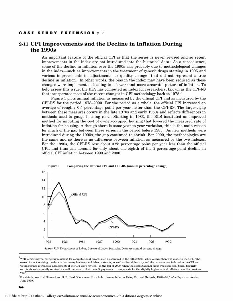
C A S E S T U D Y E X T E N S I O N p. 35
2-11 CPI Improvements and the Decline in Inflation During the 1990s
An important feature of the official CPI is that the series is never revised and so recentimprovements in the index are not introduced into the historical data.1 As a consequence,some of the decline in inflation over the 1990s was probably due to methodological changesin the index—such as improvements in the treatment of generic drugs starting in 1995 andvarious improvements in adjustments for quality change—that did not represent a truedecline in inflation. In other words, the bias in the index may have been reduced as thesechanges were implemented, leading to a lower (and more accurate) picture of inflation. Tohelp assess this issue, the BLS has computed an index for researchers, known as the CPI-RSthat incorporates most of the recent changes in CPI methodology back to 1978.2
Figure 1 plots annual inflation as measured by the official CPI and as measured by theCPI-RS for the period 1978–2000. For the period as a whole, the official CPI increased anaverage of roughly 0.5 percentage point per year faster than the CPI-RS. The largest gapbetween these measures occurs in the late 1970s and early 1980s and reflects differences inmethods used to gauge housing costs. Starting in 1983, the BLS instituted an improvedmethod for imputing the cost of owner-occupied housing that lowered the measured rate ofinflation for housing. Although there is some year-to-year variation, this is the main reasonfor much of the gap between these series in the period before 1983. As new methods wereintroduced during the 1990s, the gap continued to shrink. For 2000, the methodologies arethe same and so there is no difference between inflation as measured by the two indexes.For the 1990s, the CPI-RS rose about 0.25 percentage point per year less than the officialCPI, and thus can account for only about one-eighth of the 2-percentage-point decline inofficial CPI inflation between 1990 and 2000.
44
0
2
4
6
8
10
12
14
16
1978 1981 1984 1987 1990 1993 1996 1999
Offical CPI
CPI-RS
Figure 1 Comparing the Official CPI and CPI-RS (annual percentage change)
Source: U.S. Department of Labor, Bureau of Labor Statistics. Data are annual percent change.
1Well, almost never, excepting revisions for computational errors, such as occurred in the fall of 2000, when a correction was made to the CPI. Thereason for not revising the data is that many business and labor contracts, as well as Social Security and the tax code, are indexed to the CPI andwould require retroactive adjustments if the CPI were revised. In the fall of 2000, when the computational error was corrected, Social Securityrecipients subsequently received a small increase in their benefit payments to compensate for the slightly higher rate of inflation over the previousyear.
2For details, see K. J. Stewart and S. B. Reed, “Consumer Price Index Research Series Using Current Methods, 1978-–98,” Monthly Labor Review,June 1999.
Full file at http://TestbankCollege.eu/Solution-Manual-Macroeconomics-7th-Edition-Gregory-Mankiw
L E C T U R E S U P P L E M E N T
2-12 Alternative Measures of UnemploymentThe text defines unemployment as the percentage of the labor force unemployed at aparticular time. The labor force consists of individuals 16 and over who currently have a job(the employed) or do not have a job but are actively seeking work (the unemployed). Anindividual who does not have a job and is not looking for work is not considered part of thelabor force.
While this is the most widely used measure of the unemployment rate, it is not the onlyone. The Bureau of Labor Statistics, the U.S. government agency responsible for thecollection and dissemination of unemployment data, publishes six different measures oflabor underutilization.1 These are detailed below:
U1: Persons unemployed 15 weeks or longer, as a percentage of the civilian labor force.
U2: Persons who have lost their job or have completed temporary assignments and arecurrently without a job, as a percentage of the civilian labor force.
U3: All unemployed persons, as a percentage of the civilian labor force.
U4: All unemployed persons plus discouraged workers, as a percentage of the civilianlabor force plus discouraged workers.
U5: All unemployed persons plus all marginally attached workers, as a percentage of thecivilian labor force plus all marginally attached workers.
U6: All unemployed persons plus all marginally attached workers, plus all personsemployed part time for economic reasons, as a percentage of the civilian labor forceplus all “marginally attached” workers.
U3 is known as the official unemployment rate and corresponds to the definition of theunemployment rate given in the text. U1 and U2 examine a subset of the unemployed as apercentage of the civilian labor force. U1 provides a measure of the long-term unemployed,while U2 concentrates on those who previously held jobs but now are unemployed. U3, incontrast, includes both those who have previously held jobs and those who have never held ajob but are looking for work. Figure 1 shows the unemployment rate as measured by U1 andU3 over the period 1960–2008.
The remaining three measures of labor underutilization expand the concept ofunemployment and hence the labor force to include those who are not currently searching forwork or who are working fewer hours than desired. Discouraged workers are those who wantto work and are available for work but have given up searching because they don’t believethey can find a job. Marginally attached workers, a category which includes discouragedworkers, are individuals who want to work and are available for work but are not searchingfor a job. The reasons a marginally attached worker might not be searching includesdiscouragement, transportation problems, and child-care problems. U4 and U5 thus measurethe extent to which the economy is not utilizing potential labor resources. U6 measures theextent to which both potential (the marginally attached workers) and existing (part-timeworkers who would like to work full time) labor resources are not utilized.
As shown in Figure 2, these three measures follow the cyclical pattern of the officialunemployment rate (U3), falling during the expansion of the 1990s and rising during therecessions of 2001 and 2008. In addition, Figure 2 also shows some widening in the gapbetween the broadest measure, U6, and the official measure, U3, during and immediatelyfollowing the recent recession. Unfortunately, these broad measures of unemployment areonly available since 1994, and so it is not possible to determine whether this gap has alsowidened during previous recessions.
45
1For more information, see J. E. Bregger and S. E. Haugen, “BLS Introduces New Range of Alternative Unemployment Measures,” Monthly LaborReview (October 1995): 19–26. See also the discussion in Chapter 6 of the text on p. 176.
Full file at http://TestbankCollege.eu/Solution-Manual-Macroeconomics-7th-Edition-Gregory-Mankiw
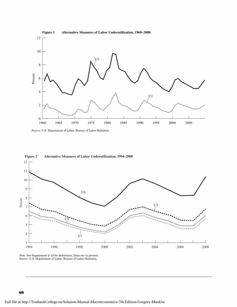
46
Figure 2 Alternative Measures of Labor Underutilization, 1994–2008
12
11
7
8
Perc
ent
9
10
5
4
6
31994 1996 1998 2000 2004
U6
2002 20082006
U5
U3
U4
Figure 1 Alternative Measures of Labor Underutilization, 1960–2008
12
10
6
Perc
ent
8
2
4
01960 1965 1970 1975 1980 1985 1990 2000 2005
U3
1995
U1
Source: U.S. Department of Labor, Bureau of Labor Statistics.
Note: See Supplement 2–12 for definitions. Data are in percent.Source: U.S. Department of Labor, Bureau of Labor Statistics.
Full file at http://TestbankCollege.eu/Solution-Manual-Macroeconomics-7th-Edition-Gregory-Mankiw
47
A D D I T I O N A L C A S E S T U D Y
2-13 Improving the National AccountsEconomists have long been aware that the statistics in the national accounts are imperfect.Some of these imperfections simply have to do with the difficulties of precisely definingand/or measuring the variables that economists care about. Some critics charge, however,that there are fundamental problems with the system of national accounts. One set ofarguments challenges the presumption that measures of income, such as Gross DomesticProduct, tell us anything useful about individuals’ welfare or overall well-being. Another setof arguments holds that the national accounts are dangerously misleading because they failto take account of the depletion of natural resources and other environmental concerns.
In the late 1960s and early 1970s, a number of commentators questioned thedesirability of economic growth—that is, increasing GDP—because they felt that increasesin GDP did not reflect increases in welfare.1 The economists William Nordhaus and JamesTobin acknowledged this possibility and, in a paper written in 1972, attempted to constructa measure of economic welfare (MEW) that adjusted for some of the differences between GDPand welfare.2 Their aim was to construct “a comprehensive measure of the annual realconsumption of households” where consumption “is intended to include all goods andservices, marketed or not . . . and allowance is to be made for negative externalities, such asthose due to environmental damage. . . .”3
This ambitious new measure thus focused on consumption. It added some components ofgovernment expenditures, such as recreation outlays, to private consumption, but not others,such as national defense (termed a “regrettable”). It reclassified some elements of privateconsumption (such as education and health expenditures and consumption of durables) asinvestment, and subtracted other components, such as personal business expenses. Nordhausand Tobin also added in an imputed value for leisure and other nonmarket uses of time.
The two most important of the many adjustments made by Nordhaus and Tobin werethe exclusion of regrettables (which they found to be an increasing fraction of GDP) and theimputations for leisure and nonmarket work. The latter correction proved to be sensitive todifferent assumptions about the effects of technical progress (technical progress allows us toproduce more goods per hour; does it also increase our enjoyment of an hour of leisuretime?). As a result, Nordhaus and Tobin could not come to a definitive conclusion aboutwhether conventional measures of economic growth understated or overstated growth inwelfare. Nevertheless, they were able to conclude that the picture of long-run economicgrowth conveyed by the national accounts is reasonably accurate; their corrected measuresof welfare all indicated long-run growth in economic well-being.
The appropriate treatment in national income accounting of natural resources andother environmental concerns was also addressed by Nordhaus and Tobin and has receivedincreased attention in recent years. The basic idea is that the national accounts shouldadjust for environmental degradation and for changes in the stocks of natural resources.
1See, for example, T. Scitovsky, The Joyless Economy (Oxford: Oxford University Press, 1976) and E. Mishan, The Costs of Economic Growth(Harmondsworth: Penguin, 1969). A recent observation along these lines, concerning the economic reforms in the Soviet Union, is the following:“Remember, even though it won’t show up positively on the national statistics, a 10 percent reduction in tanks accompanied by a 5 percent increase inmaking goods that people want is a real gain for society. . .” (Editorial, Manchester Guardian Weekly, July 21, 1991).
2W. Nordhaus and J. Tobin, “Is Growth Obsolete?” Economic Growth: Fiftieth Anniversary Colloquium V, National Bureau of Economic Research (NewYork: Columbia University Press, 1972), reprinted in J. Tobin, Essays in Economics: Theory and Policy (Cambridge, MA: MIT Press, 1985), 360–439.
3Ibid., 383.
Full file at http://TestbankCollege.eu/Solution-Manual-Macroeconomics-7th-Edition-Gregory-Mankiw

Full file at http://TestbankCollege.eu/Solution-Manual-Macroeconomics-7th-Edition-Gregory-Mankiw