chapter 1€¦ · chapter 1 general assessment ... the price of a barrel of brent crude oil is...
TRANSCRIPT

OECD Economic Outlook
Volume 2015/1
© OECD 2015
9
CHAPTER 1
GENERAL ASSESSMENT
OF THE MACROECONOMIC SITUATION

1. GENERAL ASSESSEMENT OF THE MACROECONOMIC SITUATION
10 OECD ECONOMIC OUTLOOK, VOLUME 2015/1 © OECD 2015 – PRELIMINARY VERSION
Introduction
Global growth is projected to strengthen in the course of 2015 and 2016, but will remain modest
relative to the pre-crisis period and its global distribution will change from that in recent years. The
acceleration is underpinned by very supportive monetary conditions, a slower pace of fiscal consolidation,
financial repair and lower oil prices. Investment, a crucial component to the outlook, has yet to take off.
The appreciation of the US dollar against most currencies has led to a significant realignment in exchange
rates since mid-2014. The ensuing relative price effects are shifting global demand more toward Europe,
Japan and some emerging market economies (EMEs). Growth in EMEs is slowing due to specific factors
in China, Brazil and Russia and it could continue to be weak in the absence of structural reforms to undo
bottlenecks.
Ordinary risks to the recovery path are broadly balanced around the central projection but a few
extraordinary negative event risks are not taken into account and could shift the global growth path
substantially. The projected pick-up in investment could remain elusive, but on the other hand, investment
could respond more strongly than anticipated to an upturn in spending, reduced uncertainties and recent
structural reforms, particularly in the light of low financing costs, as discussed in Chapter 3. Similarly,
compensation could accelerate more than anticipated given the continued improvements of labour market
conditions in most large OECD areas, which would support more consumption growth than projected.
However, similar expectations have failed to materialise in the past, and this pattern could continue.
Sustained quantitative easing in the euro area and Japan may prove less effective at stimulating demand
than assumed. Weakness in the first quarter in the United States and in many EMEs may signal more
underlying weakness than embedded in the projections. And oil price changes could either reduce some of
the recent real income gains that are helping to boost global demand, or add to them.
The extraordinary risks include geopolitical upheavals and severe financial instability brought about
by a disorderly exit from the zero interest rate policy in the United States, failure to reach a satisfactory
agreement between Greece and its creditors, and a hard landing in China. Avoiding these risks and moving
the global economy to a higher and more stable growth path require mutually reinforcing monetary, fiscal
and structural policies.
The outlook in a nutshell
Based on OECD assumptions (Box 1.1), growth in both OECD and non-OECD countries is projected to
pick up through 2015, after a very weak start to the year (Table 1.1 and Figure 1.1). In 2016 growth is
projected to strengthen only slightly in the OECD area, but more so in the non-OECD area (Figures 1.2
and 1.3). After turning slightly negative in early 2015, growth in the United States is projected to recover
thanks to supportive, though gradually less accommodative, monetary conditions, the dissipation of fiscal
drag, lower energy prices and an ongoing increase in household wealth. However, the pick-up will be
tempered by the stronger dollar and falling investment in the energy sector. In the euro area and Japan
activity will be supported by lower oil prices, currency depreciation and monetary policy stimulus. Fiscal
adjustment is expected to be slower in Japan and pause in the euro area, which will also support growth. In

1. GENERAL ASSESSEMENT OF THE MACROECONOMIC SITUATION
OECD ECONOMIC OUTLOOK, VOLUME 2015/1 © OECD 2015 – PRELIMINARY VERSION 11
Box 1.1. Policy and other assumptions underlying the projections
Fiscal policy settings for 2015 and 2016 are based as closely as possible on legislated tax and spending provisions. Where government plans have been announced but not legislated, they are incorporated if it is deemed clear that they will be implemented in a shape close to that announced. Where there is insufficient information to determine the allocation of budget cuts, the presumption is that they apply equally to the spending and revenue sides, and are spread proportionally across components.
In the United States the general government underlying primary balance is assumed to improve by about ½ per cent of GDP over the 2015-16 period, roughly as implied by current legislation, including the Bipartisan Budget Act and the Budget Control Act.
In Japan the projections incorporate the further 2 percentage point cut in the effective corporate income tax rate in 2015 following the cut from 37% to below 35% in 2014. The FY 2014 supplementary budget is also included. Overall, the underlying primary balance is assumed to improve by between ½ and 1 per cent of GDP in both 2015 and 2016.
In euro area countries, fiscal stances in 2015 and 2016 (measured as the change in the structural primary balance) are based on draft budget laws or, if these are not available, the stated targets in Stability Programmes.
The assumed path of policy-controlled interest rates represents the most likely outcome, conditional upon the OECD projections of activity and inflation, which may differ from those of the monetary authorities.
In the United States, the upper bound of the target federal funds rate is assumed to be raised gradually between September 2015 and December 2016 from the current level of 0.25% to 2%.
In the euro area, the main refinancing rate is assumed to be kept at 0.05% throughout the projection period.
In Japan, the short-term policy interest rate is assumed to be kept at 0.1% for the entire projection period.
In the United Kingdom, the Bank Rate is assumed to be increased gradually between February 2016 and December 2016 from the current level of 0.5% to 1.5%.
Although their impact is difficult to assess, the following quantitative-easing measures are assumed to be taken over the projection period, implicitly affecting the speed of convergence of long-term interest rates to their reference rates. In the United States and the United Kingdom the stocks of purchased assets are assumed to be maintained unchanged until the end of the projection period. In Japan asset purchases are assumed to continue in line with the stated objective of the monetary authorities to attain the inflation target; this is assumed to keep the long-term interest rate constant until end-2016. In the euro area current programmes of targeted longer-term refinancing operations (TLTROs) and purchases of private securities and sovereign bonds are assumed to last until end-2016, keeping long-term interest rates constant.
In the United States and the United Kingdom, 10-year government bond yields are assumed to converge slowly toward a reference rate (reached only well after the end of the projection period), determined by future projected short-term interest rates, a term premium and an additional fiscal premium. The latter premium is assumed to be 2 basis points per each percentage point of the gross government debt-to-GDP ratio in excess of 75%. The 10-year government bond yield is assumed to remain constant throughout the projection period at 0.36% in both Japan and Germany. Yield spreads with Germany in euro area countries are assumed to remain constant at their recent levels, with the exception of Greece, where they are assumed to decline gradually over the projection period.
Structural reforms that have been implemented or announced for the projection period are taken into account, but no further reforms are assumed to take place.
The projections assume unchanged exchange rates from those prevailing on 12 May 2015, with one US dollar equalling JPY 120.03, EUR 0.89 (or equivalently one euro equals 1.12 dollars) and 6.21 renminbi.
The price of a barrel of Brent crude oil is assumed to remain constant at USD 65 throughout the projection period. Non-oil commodity prices are assumed to be constant over the projection period at their average levels of April 2015.
The cut-off date for information used in the projections is 29 May 2015.

1. GENERAL ASSESSEMENT OF THE MACROECONOMIC SITUATION
12 OECD ECONOMIC OUTLOOK, VOLUME 2015/1 © OECD 2015 – PRELIMINARY VERSION
12http://dx.doi.org/10.1787/888933221687
Figure 1.1. Global growth is set to recover
Quarter-on-quarter percentage changes at annual rates
Source: OECD Economic Outlook 97 database.
12http://dx.doi.org/10.1787/888933220579
Table 1.1. The global recovery will gain momentum only slowly
OECD area, unless noted otherwise
Average 2014 2015 2016
2002-2011 2012 2013 2014 2015 2016 Q4 / Q4
Per cent
Real GDP growth1
World2
3.9 3.3 3.3 3.3 3.1 3.8 3.3 3.2 3.9
OECD2
1.7 1.3 1.4 1.8 1.9 2.5 1.8 2.1 2.6
United States 1.7 2.3 2.2 2.4 2.0 2.8 2.4 1.7 2.8
Euro area 1.1 -0.8 -0.3 0.9 1.4 2.1 0.8 1.8 2.2
Japan 0.7 1.7 1.6 -0.1 0.7 1.4 -0.8 1.9 1.3
Non-OECD2
6.7 5.2 5.1 4.7 4.2 4.9 4.6 4.3 5.0
China 10.6 7.7 7.7 7.4 6.8 6.7 7.2 6.7 6.6
Output gap3
0.1 -2.1 -2.2 -2.0 -1.9 -1.2
Unemployment rate4
6.9 7.9 7.9 7.3 6.9 6.6 7.1 6.8 6.5
Inflation5
2.1 1.9 1.3 1.5 0.7 1.7 1.3 0.9 1.8
Fiscal balance6
-4.4 -5.8 -4.2 -3.7 -3.1 -2.5
Memorandum Items
World real trade growth 5.6 3.1 3.3 3.2 3.9 5.3 3.6 3.9 5.9
1. Year-on-year increase; last three columns show the increase over a year earlier.
2. Moving nominal GDP weights, using purchasing power parities.
3. Per cent of potential GDP.
4. Per cent of labour force.
5. Private consumption deflator. Year-on-year increase; last 3 columns show the increase over a year earlier.
6. Per cent of GDP.
Source: OECD Economic Outlook 97 database.

1. GENERAL ASSESSEMENT OF THE MACROECONOMIC SITUATION
OECD ECONOMIC OUTLOOK, VOLUME 2015/1 © OECD 2015 – PRELIMINARY VERSION 13
Figure 1.2. Main OECD economies: macroeconomic projections
Source: OECD Economic Outlook 97 database.
12http://dx.doi.org/10.1787/888933220580
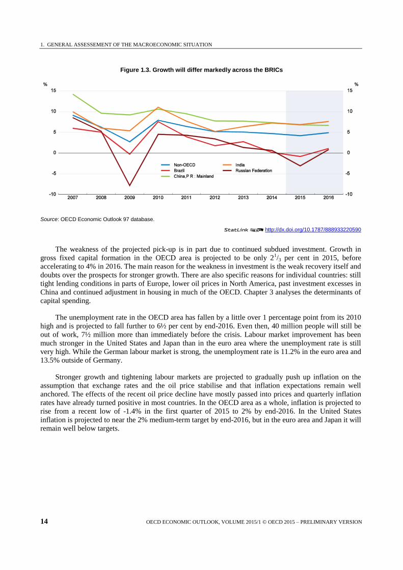
China growth is projected to edge down as the restructuring of the economy progresses, with services
taking over from investment and real estate as the main driver of economic growth. In contrast, growth is
set to pick up in the other main EMEs: the recessions in Russia and Brazil are projected to give way to low
but positive growth in 2016; growth in India will remain broadly stable in 2015 and 2016; and Indonesia’s
growth is projected to rise over the remainder of 2015 and in 2016.
1. GENERAL ASSESSEMENT OF THE MACROECONOMIC SITUATION
14 OECD ECONOMIC OUTLOOK, VOLUME 2015/1 © OECD 2015 – PRELIMINARY VERSION
Figure 1.3. Growth will differ markedly across the BRICs
Source: OECD Economic Outlook 97 database.
12http://dx.doi.org/10.1787/888933220590
The weakness of the projected pick-up is in part due to continued subdued investment. Growth in
gross fixed capital formation in the OECD area is projected to be only 21/3 per cent in 2015, before
accelerating to 4% in 2016. The main reason for the weakness in investment is the weak recovery itself and
doubts over the prospects for stronger growth. There are also specific reasons for individual countries: still
tight lending conditions in parts of Europe, lower oil prices in North America, past investment excesses in
China and continued adjustment in housing in much of the OECD. Chapter 3 analyses the determinants of
capital spending.
The unemployment rate in the OECD area has fallen by a little over 1 percentage point from its 2010
high and is projected to fall further to 6½ per cent by end-2016. Even then, 40 million people will still be
out of work, 7½ million more than immediately before the crisis. Labour market improvement has been
much stronger in the United States and Japan than in the euro area where the unemployment rate is still
very high. While the German labour market is strong, the unemployment rate is 11.2% in the euro area and
13.5% outside of Germany.
Stronger growth and tightening labour markets are projected to gradually push up inflation on the
assumption that exchange rates and the oil price stabilise and that inflation expectations remain well
anchored. The effects of the recent oil price decline have mostly passed into prices and quarterly inflation
rates have already turned positive in most countries. In the OECD area as a whole, inflation is projected to
rise from a recent low of -1.4% in the first quarter of 2015 to 2% by end-2016. In the United States
inflation is projected to near the 2% medium-term target by end-2016, but in the euro area and Japan it will
remain well below targets.

1. GENERAL ASSESSEMENT OF THE MACROECONOMIC SITUATION
OECD ECONOMIC OUTLOOK, VOLUME 2015/1 © OECD 2015 – PRELIMINARY VERSION 15
Main issues for economic prospects
Major exchange rate realignments affect macroeconomic conditions
The currencies of many advanced countries and large EMEs have depreciated noticeably against the
US dollar since mid-2014, to a similar extent as in 2008-09, despite some reversal since mid-April 2015
(Figure 1.4). In a number of economies, the depreciation vis-à-vis the dollar has been in excess of 15%,
though in nominal and real effective terms the adjustment has been less pronounced, and some countries’
currencies have even appreciated in effective terms. Consequently, the real effective exchange rate of the
US dollar has appreciated by nearly 10% since mid-2014 and slightly more in nominal terms. Smaller
effective exchange rate adjustments than bilateral changes potentially imply muted trade effects relative to
financial effects.
These currency movements have been driven by differences in monetary policy stances around the
world. Markets have been expecting a gradual tightening of monetary policy in the United States but
easing in the euro area and Japan, leading to growing interest rate differentials (Figure 1.5). As a result of
the decision by the Bank of Japan to expand quantitative and qualitative easing and a series of measures by
the European Central Bank, including the decision to purchase sovereign bonds, total assets of the major
OECD central banks have continued to expand rapidly. In addition, several central banks have reduced
policy rates due to easing inflationary pressures and a weakening economy.
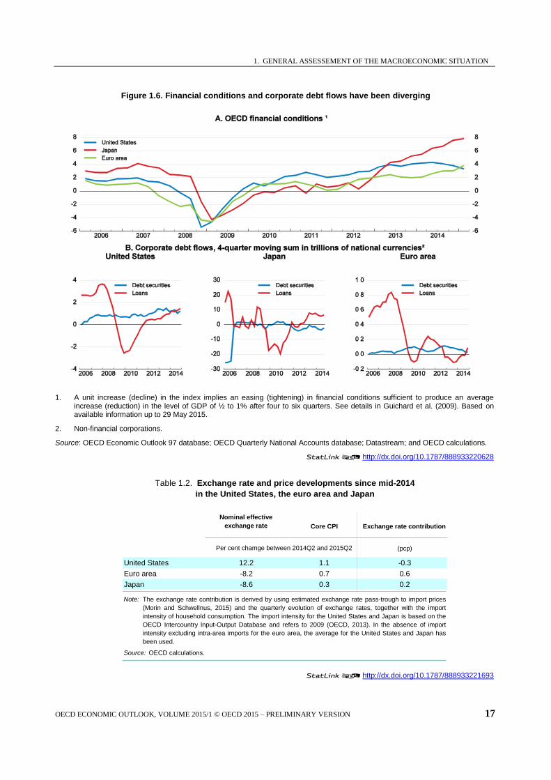
The exchange rate changes have affected financial conditions. The US dollar appreciation has
contributed to a tightening of financial conditions in the United States, while the opposite holds in the euro
area and Japan (Figure 1.6). In all three areas, bond and equity prices have increased, helped by monetary
policy support, boosting household wealth and lowering financing costs for corporations. Indeed, bond
Figure 1.4. Many currencies have depreciated against the US dollar
Per cent depreciation between July 2014 and May 2015
Note: A negative number implies a depreciation of the indicated country's currency against the US dollar (USD) and against a trade-weighted basket of currencies deflected with consumer prices (real effective exchange rate).
Source: OECD Economic Outlook 97 database; Datastream; and OECD calculations.
12http://dx.doi.org/10.1787/888933220606

1. GENERAL ASSESSEMENT OF THE MACROECONOMIC SITUATION
16 OECD ECONOMIC OUTLOOK, VOLUME 2015/1 © OECD 2015 – PRELIMINARY VERSION
Figure 1.5. Divergence in monetary policy stances has increased
Differences in 1 and 2-year ahead expected overnight interest rates vis-à-vis the United States
Note: Average differences for the months indicated.
Source: Bloomberg; and OECD calculations.
12http://dx.doi.org/10.1787/888933220614
prices rose to record highs in the euro area in mid-April, after which they fell abruptly, with the associated
increase in yields (by around 50 basis points), although bond prices still remain high. Nevertheless,
corporate debt flows from all sectors have been subdued in the euro area, although loan flows now seem to
be picking up, and in Japan. In contrast, debt flows have been rising in the United States.
The currency movements that have taken place since mid-2014 have had a marked impact on
domestic inflation. This is especially the case in the euro area where the pass-through of exchange rates to
inflation is estimated to be stronger than in the United States and Japan (Morin and Schwellnus, 2014).
Taking into account the estimated pass-through rate and the import intensity of demand, the effective
nominal depreciation of the euro since mid-2014 could directly account for the bulk of the increase in the
core consumer price level in the area since then (Table 1.2). Also, the yen depreciation over the same
period could have contributed somewhat to the increase in core consumer prices in Japan. By contrast, the
appreciation of the US dollar may on its own have held back the recovery in US inflation.
The recent exchange rate changes will affect the volume of exports and imports and reallocate
demand from the United States to the euro area and Japan. The extent of the impact depends on the pass-
through of currency changes into export and import prices and price elasticities of exports and imports. The
pass-through is estimated to be very weak in the United States for both exports and imports compared with
the euro area, and export and import price elasticities vary significantly across countries. For the United
States, the dollar’s appreciation is projected to result in losses in market shares of US exporters and an
increase in import penetration. Consequently, a cumulative negative net export contribution to growth over
2015 and 2016 of around 1¼ percentage point is projected. For the euro area and Japan, the opposite holds,
with a positive cumulative net export contribution to growth of around ½. The contribution of net exports
to growth in non-OECD economies is projected to be just below ½ percentage point (Figure 1.7).
1. GENERAL ASSESSEMENT OF THE MACROECONOMIC SITUATION
OECD ECONOMIC OUTLOOK, VOLUME 2015/1 © OECD 2015 – PRELIMINARY VERSION 17
Figure 1.6. Financial conditions and corporate debt flows have been diverging
1. A unit increase (decline) in the index implies an easing (tightening) in financial conditions sufficient to produce an average increase (reduction) in the level of GDP of ½ to 1% after four to six quarters. See details in Guichard et al. (2009). Based on available information up to 29 May 2015.
2. Non-financial corporations.
Source: OECD Economic Outlook 97 database; OECD Quarterly National Accounts database; Datastream; and OECD calculations.
12http://dx.doi.org/10.1787/888933220628
12http://dx.doi.org/10.1787/888933221693
Table 1.2. Exchange rate and price developments since mid-2014
in the United States, the euro area and Japan
Nominal effective
exchange rate Core CPI Exchange rate contribution
(pcp)
United States 12.2 1.1 -0.3
Euro area -8.2 0.7 0.6
Japan -8.6 0.3 0.2
Note:
Source: OECD calculations.
Per cent chamge between 2014Q2 and 2015Q2
The exchange rate contribution is derived by using estimated exchange rate pass-trough to import prices
(Morin and Schwellnus, 2015) and the quarterly evolution of exchange rates, together with the import
intensity of household consumption. The import intensity for the United States and Japan is based on the
OECD Intercountry Input-Output Database and refers to 2009 (OECD, 2013). In the absence of import
intensity excluding intra-area imports for the euro area, the average for the United States and Japan has
been used.

1. GENERAL ASSESSEMENT OF THE MACROECONOMIC SITUATION
18 OECD ECONOMIC OUTLOOK, VOLUME 2015/1 © OECD 2015 – PRELIMINARY VERSION
Figure 1.7. Net exports are projected to contribute negatively to growth in the United States in contrast with other areas
Sum of contribution of net exports to annual GDP growth for indicated periods
Source: OECD Economic Outlook 97 database.
12http://dx.doi.org/10.1787/888933220634
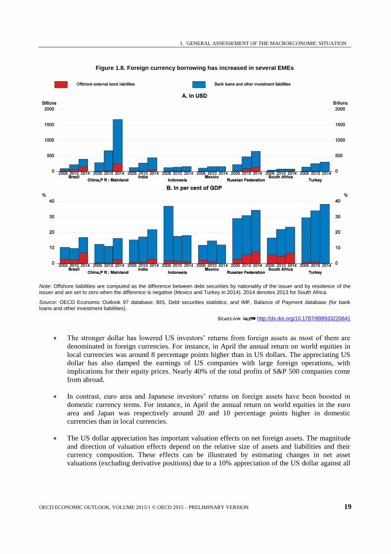
Currency movements also have financial implications stemming from international exposures:
In EMEs depreciating domestic currencies have been increasing the servicing cost of debt
denominated in foreign currencies. Foreign currency debt has risen in several large EMEs over
recent years, though such exposures appear to be lower relative to GDP than they were before the
Asian crisis in 1997 (Figure 1.8; Ollivaud et al., 2015). In particular, companies in many EMEs
have increased their foreign currency borrowing (Chui et al., 2014). The impact of a US dollar
appreciation on corporate balance sheets will depend on the extent to which loans are
denominated in US dollars and whether these currency risks are hedged. The lack of
comprehensive data precludes the drawing of firm conclusions, though in several Asian EMEs
foreign liabilities are primarily denominated in US dollars. Higher debt servicing costs may not
be a problem for companies with revenues primarily in foreign currencies, as is the case with
many commodity exporters. However, the recent decline in global commodity prices has hit
commodity producers’ revenues. Debt servicing strains would be aggravated if investors become
excessively risk averse, intensifying capital outflows. However, portfolio capital continued to
flow into EMEs until April (IIF, 2015), though this has reversed somewhat in May, and no
significant corrections in equity and debt markets in major EMEs have been observed.1 Indeed, in
China, the equity market has actually surged by more than 30% since the start of the year,
following 60% gains in the second half of 2014, despite evidence of weakness in the economy.
1. Debt servicing strains have also risen in Central and Eastern European countries. Their currencies
depreciated strongly against the Swiss franc following the decision of the Swiss National Bank to abandon
the minimum exchange rate against the euro in mid-January. Banks and households still have non-
negligible liabilities denominated in Swiss francs, which are unlikely to be hedged by households.
1. GENERAL ASSESSEMENT OF THE MACROECONOMIC SITUATION
OECD ECONOMIC OUTLOOK, VOLUME 2015/1 © OECD 2015 – PRELIMINARY VERSION 19
Figure 1.8. Foreign currency borrowing has increased in several EMEs
Note: Offshore liabilities are computed as the difference between debt securities by nationality of the issuer and by residence of the issuer and are set to zero when the difference is negative (Mexico and Turkey in 2014). 2014 denotes 2013 for South Africa.
Source: OECD Economic Outlook 97 database; BIS, Debt securities statistics; and IMF, Balance of Payment database (for bank loans and other investment liabilities).
12http://dx.doi.org/10.1787/888933220641
The stronger dollar has lowered US investors’ returns from foreign assets as most of them are
denominated in foreign currencies. For instance, in April the annual return on world equities in
local currencies was around 8 percentage points higher than in US dollars. The appreciating US
dollar has also damped the earnings of US companies with large foreign operations, with
implications for their equity prices. Nearly 40% of the total profits of S&P 500 companies come
from abroad.
In contrast, euro area and Japanese investors’ returns on foreign assets have been boosted in
domestic currency terms. For instance, in April the annual return on world equities in the euro
area and Japan was respectively around 20 and 10 percentage points higher in domestic
currencies than in local currencies.
The US dollar appreciation has important valuation effects on net foreign assets. The magnitude
and direction of valuation effects depend on the relative size of assets and liabilities and their
currency composition. These effects can be illustrated by estimating changes in net asset
valuations (excluding derivative positions) due to a 10% appreciation of the US dollar against all
1. GENERAL ASSESSEMENT OF THE MACROECONOMIC SITUATION
20 OECD ECONOMIC OUTLOOK, VOLUME 2015/1 © OECD 2015 – PRELIMINARY VERSION
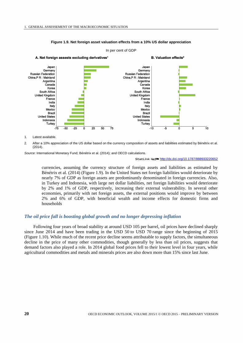
Figure 1.9. Net foreign asset valuation effects from a 10% US dollar appreciation
In per cent of GDP
1. Latest available.
2. After a 10% appreciation of the US dollar based on the currency composition of assets and liabilities estimated by Bénétrix et al. (2014).
Source: International Monetary Fund; Bénétrix et al. (2014); and OECD calculations.
12http://dx.doi.org/10.1787/888933220652
currencies, assuming the currency structure of foreign assets and liabilities as estimated by
Bénétrix et al. (2014) (Figure 1.9). In the United States net foreign liabilities would deteriorate by
nearly 7% of GDP as foreign assets are predominantly denominated in foreign currencies. Also,
in Turkey and Indonesia, with large net dollar liabilities, net foreign liabilities would deteriorate
by 2% and 1% of GDP, respectively, increasing their external vulnerability. In several other
economies, primarily with net foreign assets, the external positions would improve by between
2% and 6% of GDP, with beneficial wealth and income effects for domestic firms and
households
The oil price fall is boosting global growth and no longer depressing inflation
Following four years of broad stability at around USD 105 per barrel, oil prices have declined sharply
since June 2014 and have been trading in the USD 50 to USD 70 range since the beginning of 2015
(Figure 1.10). While much of the recent price decline seems attributable to supply factors, the simultaneous
decline in the price of many other commodities, though generally by less than oil prices, suggests that
demand factors also played a role. In 2014 global food prices fell to their lowest level in four years, while
agricultural commodities and metals and minerals prices are also down more than 15% since last June.

1. GENERAL ASSESSEMENT OF THE MACROECONOMIC SITUATION
OECD ECONOMIC OUTLOOK, VOLUME 2015/1 © OECD 2015 – PRELIMINARY VERSION 21
Figure 1.10. Commodity prices have fallen
Source: OECD Economic Outlook 97 database; and Datastream.
12http://dx.doi.org/10.1787/888933220664
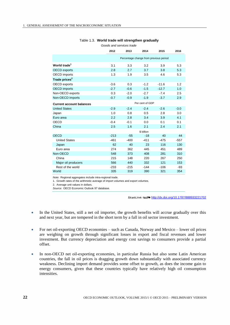
The fall in oil prices reallocates income between oil producers and consumers, both within countries
that produce oil and between net oil-exporting and net oil-importing countries. This is reflected in major
changes in current account balances (Table 1.3). The net impact of these transfers on global activity should
in itself be positive given that consumers typically have a higher spending propensity than producers. The
resulting boost in global demand is a positive development in the context of an overall deficiency of
demand. The growth benefits to net oil-importing countries will be offset to some extent by lower exports
to oil producers, as these countries have less income.2 At an oil price of USD 65 a barrel, the top ten net oil
exporters are projected to lose around USD 450 billion in export earnings this year compared with 2014.
The spending boost may take time to be realised, whereas the producer response through lowered
investment has taken place more quickly, leaving the net effect of the oil price decline somewhat muted in
the near term.
Lower oil prices will add about ¼ percentage point to both global and OECD growth in each of 2015
and 2016. The impact is estimated to be larger in Japan (about 0.6 percentage point per year) and in the
United States (about 0.4 percentage point per year including investment effects) than in the euro area
(about 0.2 percentage point per year). Despite the positive global impact, countries differ greatly in the
extent to which they are affected, given different oil consumption intensities, net oil balances and trade
exposures to energy producers (Figure 1.11).
OECD oil-importing economies with little or no oil production, such as the euro area and Japan,
receive a real income boost similar in effect to a tax cut.
2. In the 2002-08 period, re-spending rates of higher oil revenues by oil exporters are estimated to have been
around 40% for the OECD area as a whole (Wurzel et al., 2009). However, this differed significantly
across economies, with relatively low rates in the United States and Japan and relatively high ones in the
euro area countries (up to 80% in Germany).
1. GENERAL ASSESSEMENT OF THE MACROECONOMIC SITUATION
22 OECD ECONOMIC OUTLOOK, VOLUME 2015/1 © OECD 2015 – PRELIMINARY VERSION
12http://dx.doi.org/10.1787/888933221702
In the United States, still a net oil importer, the growth benefits will accrue gradually over this
and next year, but are tempered in the short term by a fall in oil sector investment.
For net oil-exporting OECD economies – such as Canada, Norway and Mexico – lower oil prices
are weighing on growth through significant losses in export and fiscal revenues and lower
investment. But currency depreciation and energy cost savings to consumers provide a partial
offset.
In non-OECD net oil-exporting economies, in particular Russia but also some Latin American
countries, the fall in oil prices is dragging growth down substantially with associated currency
weakness. Declining import demand provides some offset to growth, as does the income gain to
energy consumers, given that these countries typically have relatively high oil consumption
intensities.
Table 1.3. World trade will strengthen gradually
Goods and services trade
2012 2013 2014 2015 2016
Percentage change from previous period
World trade1
3.1 3.3 3.2 3.9 5.3
OECD exports 2.8 2.7 3.7 3.8 5.3
OECD imports 1.3 1.9 3.5 4.6 5.3
Trade prices2
OECD exports -3.6 0.3 -1.2 -11.6 1.2
OECD imports -2.7 -0.6 -1.5 -12.7 1.0
Non-OECD exports 0.3 -2.0 -2.7 -7.4 2.5
Non-OECD imports -0.7 -0.9 -1.9 -3.7 2.9
Current account balances Per cent of GDP
United States -2.9 -2.4 -2.4 -2.6 -3.0
Japan 1.0 0.8 0.5 2.8 3.0
Euro area 2.2 2.8 3.4 3.9 4.1
OECD -0.4 -0.1 0.0 0.1 0.1
China 2.5 1.6 2.1 2.4 2.1
$ billion
OECD -213 -55 -18 40 44
United States -461 -400 -411 -475 -557
Japan 62 40 23 116 130
Euro area 274 362 445 451 489
Non-OECD 548 373 408 281 310
China 215 148 220 267 250
Major oil producers 566 440 332 121 153
Rest of the world -233 -215 -144 -106 -93
World 335 319 390 321 354
Note: Regional aggregates include intra-regional trade.
1. Growth rates of the arithmetic average of import volumes and export volumes.
2. Average unit values in dollars.
Source: OECD Economic Outlook 97 database.

1. GENERAL ASSESSEMENT OF THE MACROECONOMIC SITUATION
OECD ECONOMIC OUTLOOK, VOLUME 2015/1 © OECD 2015 – PRELIMINARY VERSION 23
Figure 1.11. The oil price decline has different effects across country groups
Note: The OECD net importers group includes the Euro area, Australia, Czech Republic, Hungary, Japan, Korea, New Zealand, Poland, Sweden, Switzerland and United Kingdom. The OECD net exporters group includes Canada, Denmark, Mexico and Norway. The non-OECD net importers group includes China, India, Indonesia, Singapore, South Africa, Taiwan and a few other small countries depending on the panel, mostly in East Asia. The non-OECD net exporters group includes Russia as well as African and Middle Eastern producer countries, the precise list varying slightly between panels.
1. The results are from simulations on the National Institute of Economic and Social Research's NiGEM model, except OECD net exporters and the United States which are OECD estimates. The simulations use the observed oil price up to the end of 2015 Q1 and assume USD 65 per barrel as of 2015 Q2. The world effect is a weighted average of the five other groups.
Source: International Energy Agency; International Monetary Fund; and OECD calculations.
12http://dx.doi.org/10.1787/888933220675
Non-OECD net oil-importing economies, especially those in Asia such as India and Indonesia,
may be the greatest beneficiaries from lower oil prices as energy figures more prominently in
consumption baskets and production methods and negative net oil balances are thus relatively
large. This is also true of China, which makes greater use of coal, whose price also tumbled.
Looking ahead, even if oil prices may come under renewed downward pressure in the short term,
supply-demand projections from the International Energy Agency suggest that prices are likely to rise in
the longer term, although remain below USD 100 (Box 1.2).
1. GENERAL ASSESSEMENT OF THE MACROECONOMIC SITUATION
24 OECD ECONOMIC OUTLOOK, VOLUME 2015/1 © OECD 2015 – PRELIMINARY VERSION
Box 1.2. Potential oil price developments in the medium and longer term1
The 60% oil price drop in the second half of 2014 was not unprecedented, as similar drops happened in 1986, 1998 and 2008 (Figure below). The recent decline was both supply and demand-driven and it took place while energy markets have been undergoing fundamental changes. The International Energy Agency (IEA) expects the market rebalancing to be quite swift, but relatively limited in scope. Oil prices are expected to stabilise above current levels, but substantially below the average price of USD 110 per barrel seen in the three years preceding the drop, under the assumption that no unexpected supply disruption or major policy change takes place.
The major factors behind these price development expectations are the following:
Demand growth is expected to outpace the growth of supply over the next six years (Figure below). Oil demand is expected to grow by 1.1 mb/d per year by 2020 (an increase of about 1.1% per annum), but this is a much slower pace compared with the pre-crisis period (by about 0.2 percentage point) as the global economy has been gradually becoming less oil intensive. This trend is also spreading to EMEs, with the oil intensity of China projected to fall 20% by 2020. China’s oil demand will grow at a similar pace as the aggregate of non-OECD economies (2.4% p.a.). India stands out with annual growth of 3.4%, reflecting its rapid population and economic growth. Nevertheless, the EMEs aggregate will no longer provide as big an offset to the projected decline of demand of the OECD economies (by 0.2% p.a.) as was the case before the crisis. Among the OECD economies, the United States is the only country for which demand growth is projected (0.3% p.a.), while Japanese demand is projected to decline by 1.4% p.a. and that of OECD Europe by 0.7% p.a. in the medium term. Across all economies, fuel switching to natural gas, nuclear, coal and renewables is expected to cut global oil demand by about 2% by 2020.
Supply capacity is projected to increase by 0.86 mb/d by 2020 (about 0.9% p.a.), but at a slower pace than in the past and compared with demand, mainly due to the scaling back of investment following the drop in prices. Despite OPEC’s decision to defend its market share, almost all of its production growth by 2020 (0.5% p.a.) is projected to come from Iraq, despite security risks, reflecting its high endowment with resources. The capacity of the United Arab Emirates and Libya is also projected to grow (by about 2% p.a.) but other OPEC producers with higher costs, lower financial reserves, and social and budgetary pressures will see stagnation or even declines. Among non-OPEC countries, the United States will remain the top source of global supply growth in barrel terms. Supply is projected to grow around 3% p.a. in the United States and Canada and 5% p.a. in Brazil. Russia’s output is expected to decline by about 0.9% p.a. by 2020, as low prices, international sanctions and a depreciating currency exacerbate the effect of natural declines at the country’s brownfields. Several other smaller producer countries – including Norway, Egypt, Colombia and Indonesia – are also expected to see declines in production over the medium term.
Over a shorter term, the timing of a lifting of sanctions on Iran will affect market rebalancing. Iran would be able to restore its full supply capacity quickly and then raise it, to about 4 mb/d by 2020 from the current 2.8 mb/d. Moreover, other producers might lift their supply as well, in an attempt to preserve market share. This would lead to a considerably less tight market which would probably rebalance at an even lower price.
In addition, the following factors could affect the volatility of the oil price over the short to medium term:
Non-OPEC supply has become more price elastic. North American Light Tight Oil (LTO) has become the single largest source of global supply growth, with projected growth of about 0.3 mb/d (6%) p.a. by 2020. OPEC’s decision not to cut production in November 2014 has turned LTO into a critical market-balancing factor. LTO is more responsive both to higher and lower prices, with short lead times, faster payback and lower upfront costs, and will thus limit global under and overshooting of market corrections.
On the other hand, North America’s growing supply means that an increasing portion of its demand will be sourced locally. This will contribute to the decline in international crude trade, in particular inter-regional trade, which will also be affected by increasing volumes of crude being refined locally before being exported. Global oil trade will thus shift from crude oil to oil products, with a contraction and fragmentation in crude markets mirrored by expansion and globalisation in oil product markets. This might add to crude price volatility over the short to medium term.

1. GENERAL ASSESSEMENT OF THE MACROECONOMIC SITUATION
OECD ECONOMIC OUTLOOK, VOLUME 2015/1 © OECD 2015 – PRELIMINARY VERSION 25
Box 1.2. Potential oil price developments in the medium and longer term (Cont.)
Past and projected developments in the oil market
1. Values for 2014 episode from June 2015 onwards are Brent futures as of 27 May 2015. Futures prices are not price projections.
2. OPEC is not included in the non-OECD supply aggregate.
Source: OECD National Accounts Database; International Energy Agency; Wall Street Journal Markets Data Center; and OECD calculations.
12http://dx.doi.org/10.1787/888933220794
___________
1. This box is based on IEA (2015) and monthly IEA Oil Market Reports from 2015.

1. GENERAL ASSESSEMENT OF THE MACROECONOMIC SITUATION
26 OECD ECONOMIC OUTLOOK, VOLUME 2015/1 © OECD 2015 – PRELIMINARY VERSION
Figure 1.12. Inflation expectations have picked up
1. Expected average annual inflation based on inflation swaps. For instance, for 5-10 years ahead, this is the difference between 5-year and 10-year inflation swaps.
2. Expected inflation implied by the yield differential between 10-year government benchmark bonds and 10-year inflation-indexed bonds.
3. Average of 6-10-year ahead inflation forecast by professional forecasters from Consensus Economics.
Source: Datastream; FactSet; and Consensus Economics.
12http://dx.doi.org/10.1787/888933220680
The direct impact of oil price movements on global inflation is estimated to be essentially a one-off,
peaking after three to five months, before fading gradually. In light of the arrest to the very large fall in
commodity prices that took place in the second half of 2014 and early 2015, and the partial rebound in oil
prices since March, this implies that headline inflation rates have already troughed. Indeed, monthly global
consumer price inflation has picked up to 0.2-0.3% in recent months. The second-round effects, via wages
or the use of oil as an input into the production of other goods and services, of the oil price drop appear to
have been modest so far. Medium-term inflation expectations have either been little affected, particularly
in the case of survey-based measures, or their initial decline after the beginning of the oil price fall has
since partly reversed, notably those based on the prices of financial instruments in Japan (Figure 1.12).
Labour markets are gradually healing
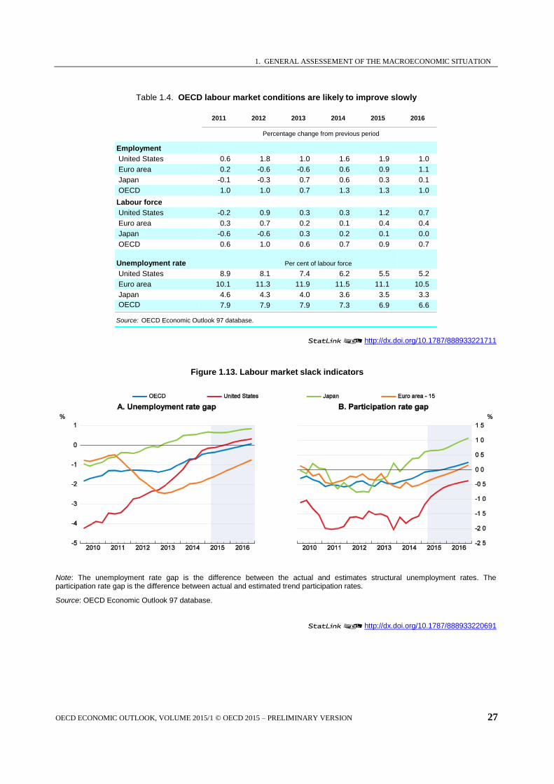
Conventional indicators suggest that slack in labour markets in advanced economies is diminishing
(Table 1.4 and Figure 1.13). At the level of the OECD as a whole, the unemployment rate has fallen to 7%,
a level not seen since 2008 and close to the estimated structural rate. This is particularly true in the United
States and Japan, although in the United States involuntary part-time work is still high and some of those
now out of the labour force might return if job prospects improve. In the euro area, by contrast,
unemployment is still quite high, with the notable exception of Germany, and involuntary part-time work is
pervasive. Narrowing gaps between actual and trend participation rates in many countries, partly reflecting
population ageing, which pushes down trend rates, is another sign of lower labour market slack.3
3. Pension reform in a number of countries may offset the effect of ageing on trend participation rates to some
extent. Already legislated reforms are taken into account in OECD long-term projections of participation
rates (see Box 4.6 in OECD, 2014a) although the offsets may be stronger than projected and more reforms
may occur.
1. GENERAL ASSESSEMENT OF THE MACROECONOMIC SITUATION
OECD ECONOMIC OUTLOOK, VOLUME 2015/1 © OECD 2015 – PRELIMINARY VERSION 27
12http://dx.doi.org/10.1787/888933221711
Figure 1.13. Labour market slack indicators
Note: The unemployment rate gap is the difference between the actual and estimates structural unemployment rates. The participation rate gap is the difference between actual and estimated trend participation rates.
Source: OECD Economic Outlook 97 database.
12http://dx.doi.org/10.1787/888933220691
Table 1.4. OECD labour market conditions are likely to improve slowly
2011 2012 2013 2014 2015 2016
Percentage change from previous period
Employment
United States 0.6 1.8 1.0 1.6 1.9 1.0
Euro area 0.2 -0.6 -0.6 0.6 0.9 1.1
Japan -0.1 -0.3 0.7 0.6 0.3 0.1
OECD 1.0 1.0 0.7 1.3 1.3 1.0
Labour force
United States -0.2 0.9 0.3 0.3 1.2 0.7
Euro area 0.3 0.7 0.2 0.1 0.4 0.4
Japan -0.6 -0.6 0.3 0.2 0.1 0.0
OECD 0.6 1.0 0.6 0.7 0.9 0.7
Unemployment rate Per cent of labour force
United States 8.9 8.1 7.4 6.2 5.5 5.2
Euro area 10.1 11.3 11.9 11.5 11.1 10.5
Japan 4.6 4.3 4.0 3.6 3.5 3.3
OECD 7.9 7.9 7.9 7.3 6.9 6.6
Source: OECD Economic Outlook 97 database.

1. GENERAL ASSESSEMENT OF THE MACROECONOMIC SITUATION
28 OECD ECONOMIC OUTLOOK, VOLUME 2015/1 © OECD 2015 – PRELIMINARY VERSION
Figure 1.14. Labour compensation
Source: OECD Economic Outlook 97 database.
12http://dx.doi.org/10.1787/888933220706
The improvement in labour markets has so far not been accompanied by a significant pick-up in wage
growth (Figure 1.14). Subdued wage growth has encouraged producers to use more labour, but has also
pushed up the profit share in some economies, including the United States. With labour markets now
getting tighter, the pendulum seems set to swing gradually away from profits and toward wages. In the
United States, compensation growth is projected to rise from about 2½ per cent now to 31/3 per cent by
end-2016. Surveys show expectations of increasing compensation, a few high-profile and large employers
have announced wage increases, and minimum wages have been raised in some states. In Japan the annual
spring negotiations point to rising base pay, and wages are projected to be rising 2¾ per cent by end-2016,
a rapid rate by Japanese standards. In Europe, however, persistently high unemployment will prevent
wages from accelerating markedly. An exception is Germany where wages are already rising at a healthy
clip and recent wage negotiations point to continued increases.
Gains in real disposable income have had a limited impact on personal consumption
Despite tepid nominal wage growth up to now, real disposable income received a fillip from the
collapse in oil and other commodity prices, which produced a large but temporary disinflationary impulse
in the global economy. From July 2014 to January 2015, the average monthly change in the global CPI was
zero. Consumer prices in advanced countries even saw outright declines in November and December 2014
and January 2015 (Figure 1.15). Together with slowly improving labour markets, this negative price
impulse inflated real wages and real disposable income. In the United States modest and stable average
hourly wage growth of around 2% at the turn of the year still translated into an acceleration in real wages.
By March 2015 real personal disposable income was up 3.3% from a year ago. The benefit to US
consumers from lower energy prices is estimated to be equivalent to a tax cut in excess of USD 500 per
household, with the impact concentrated on lower-income households, who have a higher marginal
propensity to consume. The purchasing power lift to euro area or Japanese households is more modest than
in the United States, given euro and yen weakness and lower oil consumption intensity, but it is still
significant.

1. GENERAL ASSESSEMENT OF THE MACROECONOMIC SITUATION
OECD ECONOMIC OUTLOOK, VOLUME 2015/1 © OECD 2015 – PRELIMINARY VERSION 29
Figure 1.15. Monthly inflation rates
Month-on-month percentage changes at annual rates
Source: OECD Economic Outlook 97 database; Statistics Bureau of Japan; and OECD calculations.
12http://dx.doi.org/10.1787/888933220714
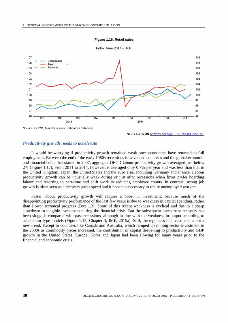
Consumers have responded unevenly to their increased purchasing power. A strong consumer
response began to build in the last quarter of 2014, with global retail sales volumes jumping 6.6% at an
annualised pace in the three months to December, including more than 3% in the euro area (Figure 1.16).
Strong consumer spending in the euro area was also supported by a surge in consumer confidence, lower
bank lending rates for households and an easing in credit conditions. In the United States real consumer
spending growth also accelerated strongly in the second half of 2014 to an annual rate above 4%. But while
retail sales volumes in the euro area look set to post a similar 3% annualised gain in the first quarter
of 2015, globally they have decelerated sharply, with barely any growth estimated in the first quarter
of 2015. In the United States real consumer spending grew only 1.8% on an annualised basis in the first
quarter despite a 5.3% gain in real disposable income. Some of the early-year weakness in the United
States can probably be attributed to bad weather effects rather than a permanently higher saving rate.
Consumer spending should thus pick up in the coming months, supported by robust labour income, low
interest rates, strong sentiment and the gradual pass-through of the stronger dollar into consumer prices.
The early-year slowdown in consumer spending in other parts of the world represents more of a puzzle but
is also expected to reverse following relatively strong fundamentals in labour markets, wealth effects,
purchasing power and sentiment.
Sustained consumption growth depends on rising wages, so the prospect of cyclical increases in real
wages is a welcome sign. Wages constitute the core of household income, especially of low-income
households with high spending propensities, and other types of income, such as pensions, are tied to wage
dynamics. Higher wages would boost sales, hiring and investment and in turn lead to higher employment
and more income in a virtuous circle. But for higher wage growth itself to be sustainable and not eaten up
by inflation, labour productivity growth must also rise.
1. GENERAL ASSESSEMENT OF THE MACROECONOMIC SITUATION
30 OECD ECONOMIC OUTLOOK, VOLUME 2015/1 © OECD 2015 – PRELIMINARY VERSION
Figure 1.16. Retail sales
Index June 2014 = 100
Source: OECD, Main Economic Indicators database.
12http://dx.doi.org/10.1787/888933220720
Productivity growth needs to accelerate
It would be worrying if productivity growth remained weak once economies have returned to full
employment. Between the end of the early 1980s recessions in advanced countries and the global economic
and financial crisis that started in 2007, aggregate OECD labour productivity growth averaged just below
2% (Figure 1.17). From 2011 to 2014, however, it averaged only 0.7% per year and was less than that in
the United Kingdom, Japan, the United States and the euro area, including Germany and France. Labour
productivity growth can be unusually weak during or just after recessions when firms prefer hoarding
labour and resorting to part-time and shift work to reducing employee counts. In contrast, strong job
growth is often seen as a recovery gains speed and it becomes necessary to rehire unemployed workers.
Faster labour productivity growth will require a boost in investment, because much of the
disappointing productivity performance of the last few years is due to weakness in capital spending, rather
than slower technical progress (Box 1.3). Some of this recent weakness is cyclical and due to a sharp
slowdown in tangible investment during the financial crisis. But the subsequent investment recovery has
been sluggish compared with past recessions, although in line with the weakness in output according to
accelerator-type models (Figure 1.18; Chapter 3; IMF, 2015a). Still, the tepidness of investment is not a
new trend. Except in countries like Canada and Australia, which ramped up mining sector investment in
the 2000s as commodity prices increased, the contribution of capital deepening to productivity and GDP
growth in the United States, Europe, Korea and Japan had been slowing for many years prior to the
financial and economic crisis.

1. GENERAL ASSESSEMENT OF THE MACROECONOMIC SITUATION
OECD ECONOMIC OUTLOOK, VOLUME 2015/1 © OECD 2015 – PRELIMINARY VERSION 31
Figure 1.17. Labour productivity and investment
Source: OECD Economic Outlook 97 database.
12http://dx.doi.org/10.1787/888933220736
Figure 1.18. Real business investment growth has been weak compared with previous cycles
Peak in OECD real investment = 100
Note: Data are for OECD countries for which the breakdown of investment is available. For the March 2008 series, the dotted line is based on projections.
Source: OECD Economic Outlook 97 database; and OECD calculations.
12http://dx.doi.org/10.1787/888933220744

1. GENERAL ASSESSEMENT OF THE MACROECONOMIC SITUATION
32 OECD ECONOMIC OUTLOOK, VOLUME 2015/1 © OECD 2015 – PRELIMINARY VERSION
Box 1.3. The contribution of weaker investment to slower potential growth
The growth rate of OECD potential output per capita, proxying the trend growth rate of living standards, slowed from just below 1½ per cent per annum in the years preceding the crisis, to below 1% in the years immediately following it, before recovering to about 1% more recently (Figure below). The slowdown can be split into contributions from potential employment and trend productivity. The growth contribution from potential employment has slowed gradually due to the effect of ageing populations and more abruptly in the years following the crisis as structural unemployment rates is some countries rose. The slowdown in trend productivity is, however, much more important in explaining the decline in potential growth, with prolonged weakness in investment an important part of the story.
The decline in trend productivity growth can be split into contributions from total factor productivity and capital per worker, assuming an underlying Cobb Douglas production form for potential output. On this basis OECD total factor productivity growth slowed following the crisis, but has since recovered close to pre-crisis growth rates. Conversely the contribution from capital per worker slowed during the crisis and has remained subdued due to the prolonged weakness in investment. Indeed, the slower growth in capital per worker explains more than half, or about 0.3% per annum, of the slowdown in trend living standards for recent years compared to pre-crisis averages. This contribution from the slowdown in capital has become more apparent with the recent revision of capital stock data to be consistent with the new system of national accounts and the associated revision to the definition of investment, which now includes expenditures on research and development.
The foregoing analysis relates to the aggregate OECD, but nearly all OECD countries have experienced a prolonged post-crisis slowdown in the contribution of capital per worker to trend productivity growth, the only exceptions being Australia, Canada and Chile, which experienced strong mining-related investment in the wake of booming commodity prices.
The slowdown in capital per worker was greatest among those countries most severely affected by the crisis. For Estonia, Greece, Iceland and Portugal the slowdown in capital per worker contributed to a slowdown in post-crisis potential growth averaging between ½ and 1 per cent per annum.
Other countries for which the post-crisis slowdown in capital per worker contributed between ¼ and ½ per cent per annum to lower potential growth are Austria, Denmark, Hungary, Italy, Japan, Korea, Luxembourg, Slovenia, Switzerland, the United Kingdom and the United States.
Decomposition of the growth rate of OECD potential output per capita
Contribution to potential per capita growth
Note: Assuming potential output (Y*) can be represented by a Cobb-Douglas production function in terms of potential employment (N*), the capital stock (K) and labour-augmenting technical progress (E*) then y* = a (n*+e*) + (1 - a) k, where lower case letters denote logs and a is the wage share. If P is the total population and PWA the population of working age (here taken to be aged 15-74), then the growth rate of potential GDP per capita (where growth rates are denoted by the first difference, d(), of logged variables) can be decomposed into the five components depicted in the figure: d(y* - p) = a d(e)* + (1-a) d(k - n*) + d(n* - pwa) + d(pwa - p).
1. Potential employment rate refers to potential employment as a share of the working-age population (aged 15-74).
2. Active population rate refers to the share of the population of working age in the total population.
3. Percentage changes.
Source: OECD Economic Outlook 97 database.
12http://dx.doi.org/10.1787/888933220800

1. GENERAL ASSESSEMENT OF THE MACROECONOMIC SITUATION
OECD ECONOMIC OUTLOOK, VOLUME 2015/1 © OECD 2015 – PRELIMINARY VERSION 33
Private investment spending, excluding housing, is generally projected to strengthen only mildly until
end-2016 as compared with previous cyclical recoveries. This is consistent with the projected modest
acceleration in domestic and global activity, lingering uncertainty, the remaining excess capacity in many
areas and the drag on investment engendered by lower oil prices in some large economies like the United
States and Canada. As economies continue to recover, consumption growth accelerates in line with wages
and incomes, and confidence in future economic prospects strengthens, firms can be expected to increase
the pace of investment spending. A number of OECD countries have also implemented sizeable structural
reforms in the wake of the economic crisis. On average across the OECD, countries have made progress in
abolishing price controls or improving their design, streamlining administrative procedures for start-ups,
simplifying rules and procedures and improving access to information about regulations. As these reforms
bear fruit, output and investment should accelerate. Moreover, the boost to investment and growth in one
country spills over to support investment and growth in others. Hence revived growth prospects,
particularly in the euro area and Japan, could disproportionately boost global growth relative to the last
several years when these areas have lagged. Such a collective response could boost the current low-level
growth equilibrium to a higher sustained growth equilibrium.
Structural policy along a number of dimensions is essential to ensuring an increase in potential growth
that is equitably shared. In this regard, the pace of structural reforms has slowed across the OECD in the
past two years, in particular as concerns product market regulation, even as it has accelerated in large non-
OECD economies (Koske et al., 2015; OECD, 2015a). Recent performance notwithstanding, a number of
economies still suffer from structural impediments and would thus benefit from further policy action:
Within the euro area, completing the Single Market with reference to the network infrastructures
of telecommunications, energy transport and digital technology would boost investment and
growth, as would further progress on banking and capital markets unions.
Boosting competition and innovation and facilitating the entry of new firms would smooth the
reallocation of labour and capital across firms and sectors and would help raise productivity
growth. In the euro area periphery, product market reforms, especially in services, are needed to
reap the full benefits of the labour market reforms introduced in recent years.
Better integration of social protection and active labour market policies would facilitate job
creation and matching and thus accelerate the elimination of labour market slack and the pick-up
in wage growth. It would also reduce labour market duality and informality.
In EMEs better physical and legal infrastructure can help address growth bottlenecks, reduce
financial sector vulnerabilities and improve resource allocation, ultimately helping to narrow the
gap in material living standards with advanced economies.
In advanced and emerging market economies alike, the ultimate drivers of productivity gains are
skills and knowledge-based human capital, underscoring the importance of raising the quality and
inclusiveness of education systems.
Risks to the outlook
The current projections for modest OECD and world recoveries describe a most likely scenario with
roughly symmetrical risks around it, including:
The projected pick-up in investment in advanced countries may fail to materialise. If investment
growth in the OECD area stayed at its 2014 level (2.7%) instead of gradually increasing to 4.7%
by end-2016 as projected, OECD area growth would be about 0.2 percentage point weaker than
1. GENERAL ASSESSEMENT OF THE MACROECONOMIC SITUATION
34 OECD ECONOMIC OUTLOOK, VOLUME 2015/1 © OECD 2015 – PRELIMINARY VERSION
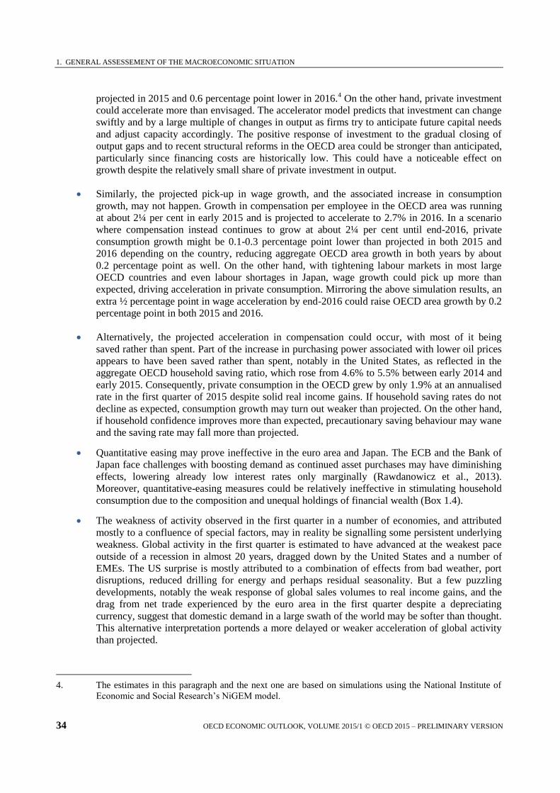
projected in 2015 and 0.6 percentage point lower in 2016.4 On the other hand, private investment
could accelerate more than envisaged. The accelerator model predicts that investment can change
swiftly and by a large multiple of changes in output as firms try to anticipate future capital needs
and adjust capacity accordingly. The positive response of investment to the gradual closing of
output gaps and to recent structural reforms in the OECD area could be stronger than anticipated,
particularly since financing costs are historically low. This could have a noticeable effect on
growth despite the relatively small share of private investment in output.
Similarly, the projected pick-up in wage growth, and the associated increase in consumption
growth, may not happen. Growth in compensation per employee in the OECD area was running
at about 2¼ per cent in early 2015 and is projected to accelerate to 2.7% in 2016. In a scenario
where compensation instead continues to grow at about 2¼ per cent until end-2016, private
consumption growth might be 0.1-0.3 percentage point lower than projected in both 2015 and
2016 depending on the country, reducing aggregate OECD area growth in both years by about
0.2 percentage point as well. On the other hand, with tightening labour markets in most large
OECD countries and even labour shortages in Japan, wage growth could pick up more than
expected, driving acceleration in private consumption. Mirroring the above simulation results, an
extra ½ percentage point in wage acceleration by end-2016 could raise OECD area growth by 0.2
percentage point in both 2015 and 2016.
Alternatively, the projected acceleration in compensation could occur, with most of it being
saved rather than spent. Part of the increase in purchasing power associated with lower oil prices
appears to have been saved rather than spent, notably in the United States, as reflected in the
aggregate OECD household saving ratio, which rose from 4.6% to 5.5% between early 2014 and
early 2015. Consequently, private consumption in the OECD grew by only 1.9% at an annualised
rate in the first quarter of 2015 despite solid real income gains. If household saving rates do not
decline as expected, consumption growth may turn out weaker than projected. On the other hand,
if household confidence improves more than expected, precautionary saving behaviour may wane
and the saving rate may fall more than projected.
Quantitative easing may prove ineffective in the euro area and Japan. The ECB and the Bank of
Japan face challenges with boosting demand as continued asset purchases may have diminishing
effects, lowering already low interest rates only marginally (Rawdanowicz et al., 2013).
Moreover, quantitative-easing measures could be relatively ineffective in stimulating household
consumption due to the composition and unequal holdings of financial wealth (Box 1.4).
The weakness of activity observed in the first quarter in a number of economies, and attributed
mostly to a confluence of special factors, may in reality be signalling some persistent underlying
weakness. Global activity in the first quarter is estimated to have advanced at the weakest pace
outside of a recession in almost 20 years, dragged down by the United States and a number of
EMEs. The US surprise is mostly attributed to a combination of effects from bad weather, port
disruptions, reduced drilling for energy and perhaps residual seasonality. But a few puzzling
developments, notably the weak response of global sales volumes to real income gains, and the
drag from net trade experienced by the euro area in the first quarter despite a depreciating
currency, suggest that domestic demand in a large swath of the world may be softer than thought.
This alternative interpretation portends a more delayed or weaker acceleration of global activity
than projected.
4. The estimates in this paragraph and the next one are based on simulations using the National Institute of
Economic and Social Research’s NiGEM model.

1. GENERAL ASSESSEMENT OF THE MACROECONOMIC SITUATION
OECD ECONOMIC OUTLOOK, VOLUME 2015/1 © OECD 2015 – PRELIMINARY VERSION 35
Box 1.4. Quantitative easing and household wealth
By increasing wealth, quantitative easing (QE) can affect the consumption and investment decisions of households. However, the importance of this channel depends on the amount of financial assets, the type of assets, and how equally they are distributed within a country. This box analyses how these characteristics differ across selected OECD countries and draws tentative conclusions about the relative effectiveness of QE.
QE involves the purchase of financial assets by central banks, with the aim of increasing their price and consequently lowering their rate of return. QE adopted by OECD central banks has largely targeted sovereign and government-guaranteed bonds. However, through portfolio effects QE has also raised prices of corporate bonds and equities. In addition to direct holdings of bonds and equities, households can be exposed to financial markets through their savings with institutional investors such as pension funds. Households are also exposed to the financial system through bank deposit accounts and liabilities such as bank loans. QE and other monetary policy stimulus measures do not affect the nominal value of these, though they can affect interest received and paid by households.
By making households feel wealthier, asset price increases can induce households to consume more, especially if such increases are perceived as permanent. Increases in asset values can improve a household’s collateral, easing access to credit through balance sheet effects (Bernanke and Gertler, 1995), enabling households to invest in housing or small businesses. The effect of changes in household wealth managed by institutions (such as pension funds) on household behaviour depends on the regulatory environment which may prohibit households from drawing down wealth prior to retirement. As richer households have a lower marginal propensity to consume (Carroll et al., 2014), QE may be less effective in countries where the distribution of wealth is highly unequal.
The size, composition and distribution of household financial assets differ greatly across six large OECD economies (Table below):
Total (and directly held) financial assets are largest in relation to GDP in the United States and Japan and significantly smaller in European countries. A larger size of financial assets may make wealth effects more powerful.
The nature of financial assets varies greatly. Japanese households hold around half of financial assets in currency and deposits. Consequently, they are less influenced by QE-driven wealth effects. In contrast, US households have the greatest direct exposure to financial market instruments, making them more susceptible to changes in asset prices and thus increasing the effectiveness of QE. In EU countries exposure is largely indirect through institutions, limiting the effects of QE on household consumption.
In each country analysed the 20% wealthiest households own the majority of financial assets, with ownership in the United States being particularly concentrated, reducing the effectiveness of QE (Figure below)
1. In countries where data are available, the distribution of deposits is less skewed. With the
exception of Italy, households’ direct holdings of equities are more widespread than of bonds. Overall, wealth gains are most likely to go to households least likely to increase consumption.
Indirect exposure to financial markets via institutions is more common than direct exposure. This reduces the effects of QE on households. Pension and insurance funds tend to invest more in bonds than equities, with the exception of the United States, where their investments are more evenly matched.
Overall, it is the assets least widely held (bonds) that are directly affected by QE, with the nominal value of the most broadly held assets (deposits) unaffected. This limits the scope for QE to affect household spending. The effects of QE bond-buying programmes are likely to be more strongly felt by households in a country such as Italy, where bonds are held by more households and in larger amounts than elsewhere.
The significance of wealth effects on households’ consumption and investment will also depend on the liability side of household balance sheets. There is less cross-country variability in terms of financial liabilities as a share of GDP. This reflects the fact that since the start of the crisis UK and US households have decreased leverage, in contrast to households in the euro area and Japan, where leverage is close to historic highs. In all countries the vast bulk of financial liabilities are in the form of loans (with mortgages comprising 50-85% of loans). The available evidence suggests that although household debt is concentrated, it is less so than household assets. In the United States almost three-quarters of households have some form of debt, compared with roughly half in France, Germany and the United Kingdom, and only a quarter in Italy. Therefore, for many households with debt the benefit of QE will only be through effects on the interest rate as their financial assets are limited to deposit accounts. This in turn will depend on how easily households can reduce interest rates on their bank loans – variable rate mortgages predominate in Italy and account for roughly half of mortgages in the UK (ECB, 2009) and Japan (Ministry of Land, Infrastructure, Transport and Tourism, 2015).

1. GENERAL ASSESSEMENT OF THE MACROECONOMIC SITUATION
36 OECD ECONOMIC OUTLOOK, VOLUME 2015/1 © OECD 2015 – PRELIMINARY VERSION
Box 1.4. Quantitative Easing and Household Wealth (Cont.)
Overall, there is potential for a more important household spending channel for QE in the United States than elsewhere, as financial instruments are larger and held by more households, although their ownership is still highly concentrated. The household channel is potentially weakest in the United Kingdom due to the lack of direct exposure to financial assets (though this does preclude the effectiveness of other channels). Japan and euro area countries lie in the middle, with effects somewhat stronger in Italy.
12http://dx.doi.org/10.1787/888933221783
The cumulative distribution of total financial assets
Note: The dataset is based on household survey data from different years: Germany (2006), Italy (2004), Japan (2003), United Kingdom (2000) and the United States (2006). The different countries have different starting percentile (on the horizontal axis) from which onwards the distribution is computed.
Source: Luxembourg Wealth Study database. 12http://dx.doi.org/10.1787/888933220817
___________
1. US Survey of Consumer Finances, 2013; UK Wealth and Assets survey, 2010/2012; and The Eurosystem Household Finance and Consumption Survey. The forthcoming OECD Wealth Database (In It together: Why Less Inequality Benefits All – OECD, 2015d) contains extensive data on financial asset distributions for many OECD countries that can be used to analyse the economic implications of wealth disparities.
2. Hedged, denominated in dollars.
Characteristics of household financial balance sheets in 2013
France Germany Italy JapanUnited
Kingdom
United
States
Per cent of GDP
Financial assets 202.2 179.6 230.2 352.3 285.3 396.6
Financial liabilities 66.7 57.0 57.6 82.3 90.6 82.1
Composition of financial assets Per cent of total financial assets
Currency and deposits 30.1 40.8 31.7 52.9 27.8 12.7
Securities other than shares,
except financial derivatives1.6 4.8 18.7 2.5 0.7 7.9
Shares and other equity,
except mutual funds shares16.7 9.2 20.5 9.7 9.7 33.2
Mutual funds shares 7.1 8.5 7.2 4.7 2.1 12.1
Net equity of households in life
insurance and pension funds reserves34.7 34.5 17.6 26.0 55.5 31.3
Other financial assets 9.8 2.2 4.3 4.2 4.2 2.8
Note : 2012 used for France, Germany and Italy. Non-consolidated data is used to better demonstrate household exposures.
Source: OECD Financial Balance Sheet Accounts.
1. GENERAL ASSESSEMENT OF THE MACROECONOMIC SITUATION
OECD ECONOMIC OUTLOOK, VOLUME 2015/1 © OECD 2015 – PRELIMINARY VERSION 37
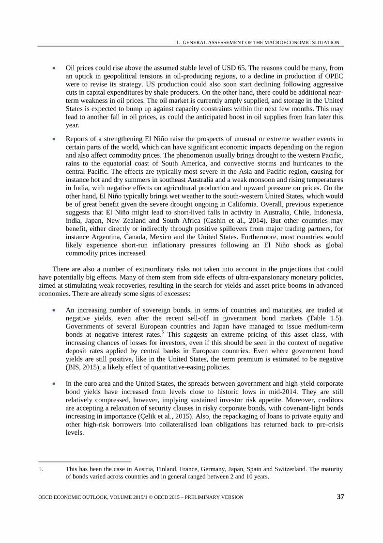
Oil prices could rise above the assumed stable level of USD 65. The reasons could be many, from
an uptick in geopolitical tensions in oil-producing regions, to a decline in production if OPEC
were to revise its strategy. US production could also soon start declining following aggressive
cuts in capital expenditures by shale producers. On the other hand, there could be additional near-
term weakness in oil prices. The oil market is currently amply supplied, and storage in the United
States is expected to bump up against capacity constraints within the next few months. This may
lead to another fall in oil prices, as could the anticipated boost in oil supplies from Iran later this
year.
Reports of a strengthening El Niño raise the prospects of unusual or extreme weather events in
certain parts of the world, which can have significant economic impacts depending on the region
and also affect commodity prices. The phenomenon usually brings drought to the western Pacific,
rains to the equatorial coast of South America, and convective storms and hurricanes to the
central Pacific. The effects are typically most severe in the Asia and Pacific region, causing for
instance hot and dry summers in southeast Australia and a weak monsoon and rising temperatures
in India, with negative effects on agricultural production and upward pressure on prices. On the
other hand, El Niño typically brings wet weather to the south-western United States, which would
be of great benefit given the severe drought ongoing in California. Overall, previous experience
suggests that El Niño might lead to short-lived falls in activity in Australia, Chile, Indonesia,
India, Japan, New Zealand and South Africa (Cashin et al., 2014). But other countries may
benefit, either directly or indirectly through positive spillovers from major trading partners, for
instance Argentina, Canada, Mexico and the United States. Furthermore, most countries would
likely experience short-run inflationary pressures following an El Niño shock as global
commodity prices increased.
There are also a number of extraordinary risks not taken into account in the projections that could
have potentially big effects. Many of them stem from side effects of ultra-expansionary monetary policies,
aimed at stimulating weak recoveries, resulting in the search for yields and asset price booms in advanced
economies. There are already some signs of excesses:
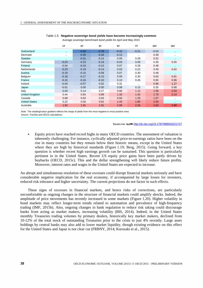
An increasing number of sovereign bonds, in terms of countries and maturities, are traded at
negative yields, even after the recent sell-off in government bond markets (Table 1.5).
Governments of several European countries and Japan have managed to issue medium-term
bonds at negative interest rates.5 This suggests an extreme pricing of this asset class, with
increasing chances of losses for investors, even if this should be seen in the context of negative
deposit rates applied by central banks in European countries. Even where government bond
yields are still positive, like in the United States, the term premium is estimated to be negative
(BIS, 2015), a likely effect of quantitative-easing policies.
In the euro area and the United States, the spreads between government and high-yield corporate
bond yields have increased from levels close to historic lows in mid-2014. They are still
relatively compressed, however, implying sustained investor risk appetite. Moreover, creditors
are accepting a relaxation of security clauses in risky corporate bonds, with covenant-light bonds
increasing in importance (Çelik et al., 2015). Also, the repackaging of loans to private equity and
other high-risk borrowers into collateralised loan obligations has returned back to pre-crisis
levels.
5. This has been the case in Austria, Finland, France, Germany, Japan, Spain and Switzerland. The maturity
of bonds varied across countries and in general ranged between 2 and 10 years.
1. GENERAL ASSESSEMENT OF THE MACROECONOMIC SITUATION
38 OECD ECONOMIC OUTLOOK, VOLUME 2015/1 © OECD 2015 – PRELIMINARY VERSION
12http://dx.doi.org/10.1787/888933221727
Equity prices have reached record highs in many OECD countries. The assessment of valuation is
inherently challenging. For instance, cyclically adjusted price-to-earnings ratios have been on the
rise in many countries but they remain below their historic means, except in the United States
where they are high by historical standards (Figure 1.19; Berg, 2015). Going forward, a key
question is whether recent high earnings growth can be sustained. This question is particularly
pertinent in in the United States. Recent US equity price gains have been partly driven by
buybacks (OECD, 2015c). This and the dollar strengthening will likely reduce future profits.
Moreover, interest rates and wages in the United States are expected to increase.
An abrupt and simultaneous resolution of these excesses could disrupt financial markets seriously and have
considerable negative implication for the real economy, if accompanied by large losses for investors,
reduced risk tolerance and higher uncertainty. The current projections do not factor in such effects.
These signs of excesses in financial markets, and hence risks of corrections, are particularly
uncomfortable as ongoing changes in the structure of financial markets could amplify shocks. Indeed, the
amplitude of price movements has recently increased in some markets (Figure 1.20). Higher volatility in
bond markets may reflect longer-term trends related to automation and prevalence of high-frequency
trading (IMF, 2015b). Also, ongoing changes in bank regulation to reduce risk taking could discourage
banks from acting as market makers, increasing volatility (BIS, 2014). Indeed, in the United States
monthly Treasuries trading volumes by primary dealers, historically key market makers, declined from
10-12% of the total stock of outstanding Treasuries prior to the crisis to just 4% recently. Large asset
holdings by central banks may also add to lower market liquidity, though existing evidence on this effect
for the United States and Japan is not clear cut (FRBNY, 2014; Kurosaki et al., 2015).
Table 1.5. Negative sovereign bond yields have become increasingly common
Average sovereign benchmark bond yields for April and May 2015
1Y 2Y 3Y 5Y 7Y 10Y 15Y
Switzerland .. -0.83 -0.78 -0.42 -0.21 -0.03 ..
Denmark .. -0.45 -0.34 -0.13 .. 0.48 ..
Sweden .. -0.31 -0.14 0.09 0.28 0.52 ..
Germany -0.24 -0.23 -0.19 -0.03 0.09 0.36 0.55
Finland -0.04 -0.19 -0.10 0.07 0.28 0.48 ..
Netherlands -0.23 -0.19 -0.14 0.03 0.22 0.49 0.62
Austria -0.19 -0.15 -0.08 0.07 0.30 0.48 ..
Belgium -0.18 -0.17 -0.10 0.09 0.30 0.60 0.81
France -0.15 -0.16 -0.10 0.10 0.26 0.65 0.96
Ireland -0.04 -0.07 0.02 0.31 .. 0.96 1.27
Japan -0.01 0.00 0.00 0.08 0.15 0.35 0.68
Italy 0.04 0.14 0.27 0.66 1.12 1.56 2.03
United Kingdom 0.44 0.65 0.89 1.33 1.42 1.79 2.14
Canada 0.68 0.63 0.63 0.94 1.25 1.57 ..
United States 0.22 0.56 0.91 1.43 1.80 2.05 ..
Australia 1.92 1.91 1.91 2.08 2.35 2.63 2.88
Note: The shading/colour gradient reflects the range of yields from the most negative to most positive ones.
Source : FactSet and OECD calculations.

1. GENERAL ASSESSEMENT OF THE MACROECONOMIC SITUATION
OECD ECONOMIC OUTLOOK, VOLUME 2015/1 © OECD 2015 – PRELIMINARY VERSION 39
Figure 1.19. Equity prices have increased
Normalised cyclically adjusted price-to-earnings ratios in standard deviations
Note: The cyclically adjusted PE ratio (CAPE ratio) is computed as the current price divided by the average inflation-adjusted earnings from the previous 10 years. The measure attempts to smooth the impact of the business cycle on earnings. Normalisation is based on the average since the early 1980s.
Source: Datastream; OECD, Main Economic Indicators database; and OECD calculations.
12http://dx.doi.org/10.1787/888933220754
Figure 1.20. Volatility in bond markets has increased
Daily difference in 10-year government bond yields over their level
1. Based on the JP Morgan Emerging Markets Global Composite Index. Bond yields refer to different maturities.
Source: Datastream; and OECD calculations. 12http://dx.doi.org/10.1787/888933220760

1. GENERAL ASSESSEMENT OF THE MACROECONOMIC SITUATION
40 OECD ECONOMIC OUTLOOK, VOLUME 2015/1 © OECD 2015 – PRELIMINARY VERSION
In this context, and given limited room for either monetary or fiscal policy support, four adverse
scenarios could have sizeable implications for the real economy with strong international spillovers.
The normalisation of US monetary policy needed for meeting inflation and employment
objectives may involve financial turmoil, with negative effects on domestic and global GDP.
The beginning of policy interest rate tightening may be accompanied by a jump in US long-
term interest rates and general asset price declines given extreme valuations of many asset
classes. A mere convergence of financial market participants’ expectations with the median
expectations of FOMC members from March, would imply that the 10-year government bond
yield increases by 1¼ percentage points to around 3¼ per cent. Much larger increases would
take place if initial declines in asset prices lead to fire sales, a drying up of liquidity and
pervasive risk aversion. In this case, it would drive down US growth unless offset by policy
measures. Given the importance of the United States for the global economy, other economies
would be affected by weaker US growth. Macro-model simulations, accounting for trade and
simple financial spillovers, suggest that a stylised increase of 200 basis points in 10-year
government bond yields combined with a 25% drop in equity prices in the United States and
several other large economies during one year would lower OECD GDP growth by more than
1 percentage point compared with the baseline (Rawdanowicz et al., 2014a).6 The impact
would be magnified if the hike in US yields were to be accompanied by a strong appreciation
of the dollar and disruptive capital outflows from EMEs, where external bank debt is
dominated by short-term debt (Annex 1.1). Given the increase in dollar borrowing by banks
and corporations in the EMEs (see above), a strong dollar appreciation could trigger financial
instability, which could be compounded by capital outflows.
Failure to reach a satisfactory agreement between Greece and its official creditors would
intensify perceptions of redenomination risks and uncertainty. Although the implications of
such an extraordinary event are impossible to predict, they would most likely involve an
aggravation again of financial fragmentation in the euro area, dampening real activity and
restarting negative feedback loops between the real economy, the banking sector and the
public finances in vulnerable euro area countries. Euro area turmoil would primarily have
negative effects on its neighbours, given strong trade and financial links. And global negative
spillovers, especially via confidence and financial links, would also be likely, involving higher
risk premia and a strong decline in financial asset prices. So far, risk premia in various
financial instruments seem to discount such a scenario. Thus, spreads in government bond
yields vis-à-vis German Bunds and sovereign credit default swap spreads have declined or
stabilised at low levels in recent months for all euro area economies but Greece, where they
have increased sizeably (Figure 1.21). Similarly, Target 2 balances for vulnerable countries,
other than Greece, have been stable or narrowed. The calm in financial markets in spite of the
mounting uncertainty may reflect low exposures of private investors to Greece. For instance,
claims of BIS reporting banks on Greece in US dollar terms are a quarter of what they were
four years ago, and sovereign debt is now mostly held by official creditors. Market calm could
also reflect a perception that the ECB measures and the stronger euro area institutional
framework would contain any serious spillover effects. However, market sentiment could
change abruptly, if Greece and its creditors fail to reach an agreement.
6. These simulations assume the same increase in government bond yields in the United States as in other
economies. This is a strong assumption. Although recent correlations of changes in 10-year government
bond yields have been very high in many OECD countries (ranging between around 0.75 and 0.95 in
Canada, France, Germany and the United Kingdom), they were still below 1 and in some countries they
were as low as 0.5 (Italy and Japan). Nevertheless, past correlations may be a poor predictor of future co-
movements.
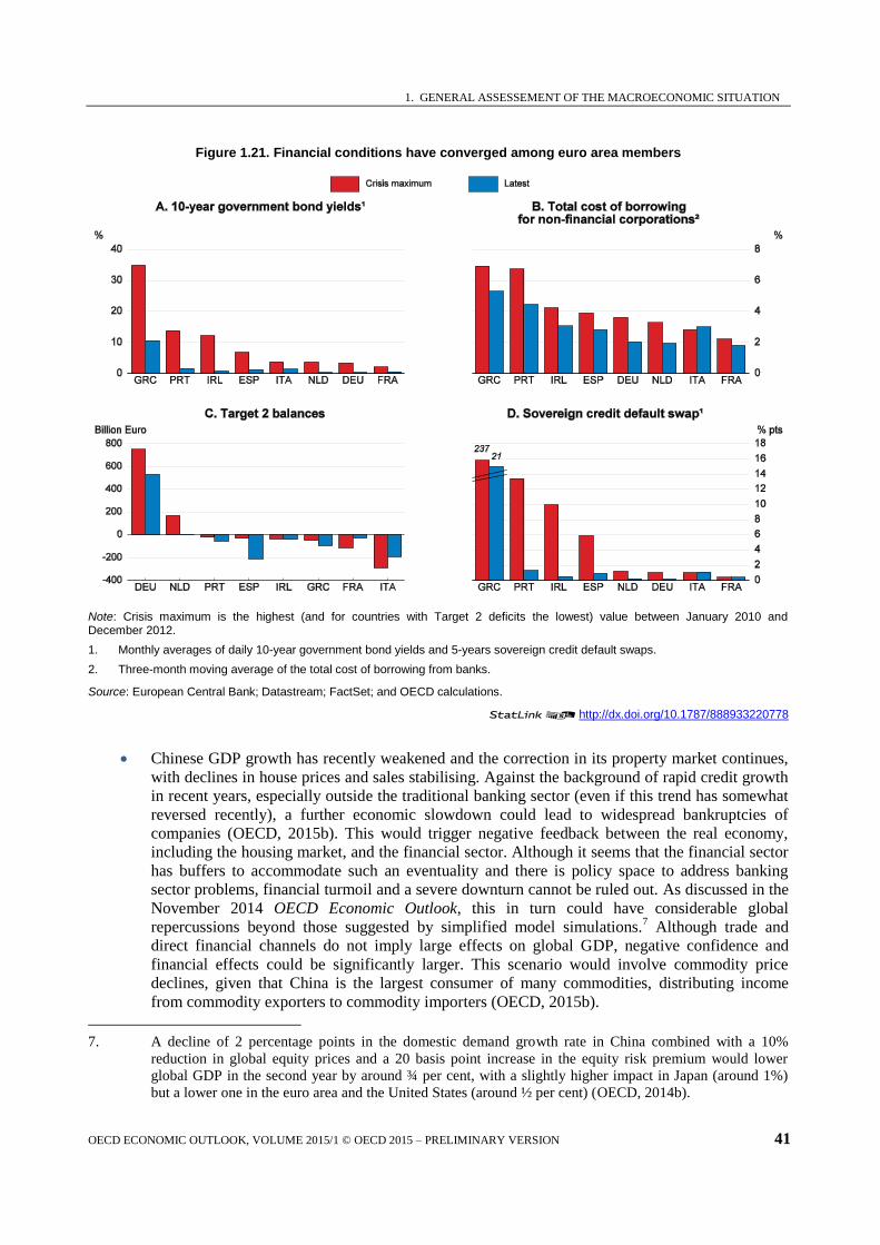
1. GENERAL ASSESSEMENT OF THE MACROECONOMIC SITUATION
OECD ECONOMIC OUTLOOK, VOLUME 2015/1 © OECD 2015 – PRELIMINARY VERSION 41
Figure 1.21. Financial conditions have converged among euro area members
Note: Crisis maximum is the highest (and for countries with Target 2 deficits the lowest) value between January 2010 and December 2012.
1. Monthly averages of daily 10-year government bond yields and 5-years sovereign credit default swaps.
2. Three-month moving average of the total cost of borrowing from banks.
Source: European Central Bank; Datastream; FactSet; and OECD calculations.
12http://dx.doi.org/10.1787/888933220778
Chinese GDP growth has recently weakened and the correction in its property market continues,
with declines in house prices and sales stabilising. Against the background of rapid credit growth
in recent years, especially outside the traditional banking sector (even if this trend has somewhat
reversed recently), a further economic slowdown could lead to widespread bankruptcies of
companies (OECD, 2015b). This would trigger negative feedback between the real economy,
including the housing market, and the financial sector. Although it seems that the financial sector
has buffers to accommodate such an eventuality and there is policy space to address banking
sector problems, financial turmoil and a severe downturn cannot be ruled out. As discussed in the
November 2014 OECD Economic Outlook, this in turn could have considerable global
repercussions beyond those suggested by simplified model simulations.7 Although trade and
direct financial channels do not imply large effects on global GDP, negative confidence and
financial effects could be significantly larger. This scenario would involve commodity price
declines, given that China is the largest consumer of many commodities, distributing income
from commodity exporters to commodity importers (OECD, 2015b).
7. A decline of 2 percentage points in the domestic demand growth rate in China combined with a 10%
reduction in global equity prices and a 20 basis point increase in the equity risk premium would lower
global GDP in the second year by around ¾ per cent, with a slightly higher impact in Japan (around 1%)
but a lower one in the euro area and the United States (around ½ per cent) (OECD, 2014b).

1. GENERAL ASSESSEMENT OF THE MACROECONOMIC SITUATION
42 OECD ECONOMIC OUTLOOK, VOLUME 2015/1 © OECD 2015 – PRELIMINARY VERSION
An escalation of the conflict between Russia and Ukraine could lead to negative confidence
effects and disruptions in energy supply, damping economic growth in EU economies (OECD,
2014b). Confidence effects could deter new investment, particularly in Germany, the Baltic
States and several Central and Eastern European economies. Protracted gas supply disruptions
would increase energy prices significantly due to switching to more expensive alternative
sources. GDP growth could also be dampened by lower exports to Russia and Ukraine, even
though these countries do not account for a large share of exports for the euro area as a whole.8
Policy requirements
Mutually reinforcing monetary, fiscal and structural policies are needed, with important cross-country
differences. There are limits to relying on a single policy instrument to boost demand, both in terms of the
scope for policy action and of how effective a single tool can be without creating imbalances in the future.
This, together with uncertainties about the effectiveness of macroeconomic policies, suggests that there is a
need to pursue wide-ranging stimulative policies. This would also allow authorities to reap positive
synergies across various policies. For instance, structural policies to stimulate investment (Chapter 3),
could strengthen not only current demand but also future potential growth. This in turn could raise neutral
real interest rates and boost the effectiveness of monetary policy (Rawdanowicz et al., 2014b). Additional
activity could also restore room for fiscal policy to better adapt to economic conditions.
Monetary policy
While remaining supportive, monetary policy stances are set to become increasingly divergent across
the key economies, as is appropriate. The gradual disappearance of slack in the United States, and the
associated prospect of inflation moving to its target, calls for gradual increases in policy rates. The timing
and pace of this withdrawal of stimulus will depend on the outlook for inflation, which in turn will depend
on the strength of the economy. In the euro area and Japan, very low inflation warrants continued
supportive monetary policy, as planned.
Large commodity and exchange rate movements complicate monetary policy setting at the current
juncture as their persistent effects on inflation and output are uncertain. With little signs of second-round
effects of oil price falls or de-anchoring of medium-term inflation expectations, and headline inflation
already recovering, monetary authorities should look through these movements and need not respond.
However, should significant second-round effects materialise, extra measures will be needed. This would
particularly be the case for the euro area and Japan, where risks of deflation are still not negligible and
second-round inflationary effects proved to be important in the past.9
Monetary policy should also look
through the direct transitory impact of currency appreciation on inflation and only respond to the extent
that second-round effects threaten an undershooting of the inflation target for a protracted period.
Similarly, in countries with already very low inflation, exchange rate depreciation should not weaken
stimulus, if following the dissipation of first-round effects inflation would still undershoot the target.
To the extent that financial markets may not have accurately incorporated the effects of a future
tightening of US monetary policy, the actual tightening may lead to financial market volatility and global
8. Simulations using the NiGEM model suggest that, at constant exchange rates, a 10% decline in Russian
imports could reduce GDP growth marginally in the OECD and the euro area, but much more for Russia’s
neighbours. If this were to be accompanied by safe-haven demand for euros and an appreciation of the
nominal euro effective exchange rate, adverse spillovers would be exacerbated. Each 5% appreciation
could reduce GDP growth in the euro area by 0.2 percentage point.
9. Indirect and second-round effects of past oil price shocks accounted on average for around a third of total
changes in inflation rates (ECB, 2010).

1. GENERAL ASSESSEMENT OF THE MACROECONOMIC SITUATION
OECD ECONOMIC OUTLOOK, VOLUME 2015/1 © OECD 2015 – PRELIMINARY VERSION 43
bond yield spillovers (see above). The need for policy response would largely depend on the relative
effects of the induced currency turbulence and of higher interest rates, and on prevailing inflation and the
monetary policy stance.
In areas where inflation is below target and GDP growth is weak, more monetary policy easing
would be desirable if the negative effects of higher bond yields materialise faster and exceed any
positive effects from currency depreciation. In the euro area and Japan, with very low interest
rates and already large asset purchases, the scope for further monetary accommodation is,
however, limited. Expanding asset purchases is feasible but may lead to still more market
distortions and be constrained in practice by the availability of bonds.10
Similarly, taking policy
rates well into negative territory could lead to costly market distortions.
In countries with high inflation and inflation expectations poorly anchored, monetary policy
should be tightened to limit capital outflows. This has already been the case in Brazil and Russia.
In some countries, concerns regarding exchange rate effects have led to easing even as inflation
remains above target (India). If short-lived foreign currency liquidity problems arise, threatening
system-wide financial stability, countries could apply for multilateral facilities, if they have
strong policy frameworks and track records in economic performance. Transparent and
temporary exchange rate interventions could also be considered to address short-term volatility,
when sufficient foreign exchange rate reserves are available. Introducing controls on capital
flows is likely to be counterproductive.
Fiscal policy
Fiscal policy is estimated to be roughly neutral in the United States and the euro area and mildly
restrictive in Japan (Table 1.6). Consideration of the near-term effects of the fiscal stance, in light of
needed growth to service debt obligations, is key. A medium-term commitment to fiscal consolidation
appears to appropriately balance the near and long term objectives. Public debt-to-GDP ratios are projected
to stabilise by 2016 in the OECD area as a whole, a decline in the ratio in the euro area offsetting an
increase in Japan and the United States (in 2015 only). However, government debt is still very high relative
to GDP in most OECD countries.
The evolution of government debt essentially depends on economic growth and interest rates going
forward, rising budgetary pressures associated with population ageing, and the design of fiscal policies,
which itself can have a significant impact on economic activity.
In most OECD countries, exceptionally low interest rates help to contain debt servicing costs at
present (Figure 1.21). Interest rates for 10-year government bonds and implicit interest rates for
servicing overall government debt are below GDP growth rates in 75% and 40%, respectively, of
the OECD countries, with the euro area economies that were hardest hit by the crisis being the
main exceptions. Interest rates are likely to rise in the medium term as the economy strengthens
and policy rates normalise. Moreover, better risk differentiation by capital markets since the
crisis might imply that lenders will demand higher risk premia than those seen in earlier years to
finance high government debt levels. Hence, there is a premium on boosting sustainable growth
rates now.
10. In particular in the euro area, the self-imposed 25% issue limit and 33% issuer limit are likely to constrain
asset purchases for some countries, resulting in a shortfall of around EUR 40 billion by September 2016
compared with the envisaged total amount (Claeys et al., 2015). These constraints would be even more
biding if asset purchase increased.

1. GENERAL ASSESSEMENT OF THE MACROECONOMIC SITUATION
44 OECD ECONOMIC OUTLOOK, VOLUME 2015/1 © OECD 2015 – PRELIMINARY VERSION
12http://dx.doi.org/10.1787/888933221734
On unchanged policies, population ageing and rising healthcare costs are set to lead to rapidly
rising spending pressure on public budgets. Public spending on healthcare, long-term care and
pensions is estimated to increase by 2½ per cent of GDP between 2015 and 2030 on average in
the OECD, with the fiscal burden differing considerably between countries (Chapter 3). The
increase in spending pressure would be even greater if the increase in healthcare costs is not
contained. Hence, both policy reforms and sustainable growth are needed.
Assuming, in a stylised scenario, that automatic stabilisers improve government finances as output
gaps close, and estimated spending pressure stemming from healthcare, long-term care and pensions
materialises without further fiscal consolidation, debt ratios would continue to rise in about two-thirds of
OECD countries, if interest rates equal GDP growth rates from 2020 onwards (Figure 1.22). Adverse debt
dynamics would be more negative if interest rates were to exceed growth rates. It is clear that increases in
potential growth rates as well as moves to address social spending pressures are crucial. Otherwise, several
countries, at least, face unsustainable fiscal developments.
Effective fiscal adjustment over the medium term requires credible multi-annual fiscal plans to chart a
path towards sustainable public finances, supported by growth, as well as to minimise the risk of
uncertainty weighing on private spending. Simple plans are likely to be more credible, because they focus
on key medium-term challenges facing public finances (Box 1.5).
Table 1.6. Fiscal positions will continue to improve
Per cent of GDP / potential GDP
2012 2013 2014 2015 2016
United States
Actual balance -9.0 -5.7 -5.0 -4.0 -3.6
Underlying balance -7.5 -4.6 -4.2 -3.3 -3.1
Underlying primary balance -4.5 -2.4 -1.5 -1.1 -1.0
Gross financial liabilities 110.5 109.2 110.1 111.4 111.1
Euro area
Actual balance -3.6 -2.9 -2.4 -2.1 -1.4
Underlying balance -2.3 -1.4 -1.0 -0.9 -0.7
Underlying primary balance 0.3 1.0 1.3 1.2 1.2
Gross financial liabilities 103.9 104.9 111.5 110.9 109.5
Japan
Actual balance -8.7 -8.5 -7.7 -6.8 -5.8
Underlying balance -8.0 -8.1 -7.2 -6.6 -5.7
Underlying primary balance -7.2 -7.4 -6.2 -5.6 -4.9
Gross financial liabilities 215.4 220.3 226.0 229.2 231.7
OECD1
Actual balance1
-5.8 -4.2 -3.7 -3.1 -2.5
Underlying balance2
-5.0 -3.5 -3.1 -2.7 -2.3
Underlying primary balance2
-2.7 -1.7 -1.1 -0.9 -0.7
Gross financial liabilities2
110.3 110.3 113.8 114.6 114.2
Note: Actual balances and liabilities are in per cent of nominal GDP. Underlying balances are in per cent of
potential GDP and they refer to fiscal balances adjusted for the cycle and for one-offs. Underlying primary
balance is the underlying balance excluding net debt interest payments.
1. Excludes Chile and Mexico.
2. Excludes Chile, Mexico and Turkey.
Source: OECD Economic Outlook 97 database.

1. GENERAL ASSESSEMENT OF THE MACROECONOMIC SITUATION
OECD ECONOMIC OUTLOOK, VOLUME 2015/1 © OECD 2015 – PRELIMINARY VERSION 45
Figure 1.22. Government debt dynamics
1. The interest rate is a weighted sum (0.25*IRS + 0.75*IRL). IRS is the 3-month market interest rate and IRL is the 10-year government bond rate.
2. In the scenario the following assumptions are made: Output gaps close until 2020, with the speed of the closing depending on the size of the gap at the end of the short-term projection period (2016) according to the relationship diff(GAP(t)) = 0.2*diff(GAP(t-1)) – 0.4*GAP(t-1), where diff() denotes year-on-year difference and GAP denotes the output gap. Primary balances improve in line with the closing output gaps using fiscal elasticities as estimated in Mourre et al. (2014) for the EU countries and Girouard and André (2005) for all the other countries. In addition, primary balances incorporate the estimated (linearised) increase in spending on health care, long-term care and pensions as reported in Table 4.5 in OECD Economic Outlook 96. Greece and Norway are not shown.
Source: OECD Economic Outlook 97 database; and OECD calculations.
12http://dx.doi.org/10.1787/888933220782
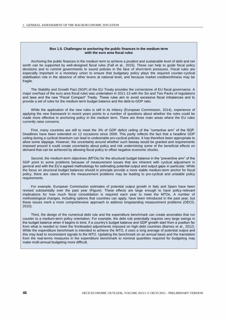
1. GENERAL ASSESSEMENT OF THE MACROECONOMIC SITUATION
46 OECD ECONOMIC OUTLOOK, VOLUME 2015/1 © OECD 2015 – PRELIMINARY VERSION
Box 1.5. Challenges to anchoring the public finances in the medium term with the euro area fiscal rules
Anchoring the public finances in the medium term to achieve a prudent and sustainable level of debt and net worth can be supported by well-designed fiscal rules (Fall et al., 2015). These can help to guide fiscal policy decisions and to commit governments to sound policies in the face of short-term pressures. Fiscal rules are especially important in a monetary union to ensure that budgetary policy plays the required counter-cyclical stabilisation role in the absence of other levers at national level, and because market creditworthiness may be fragile.
The Stability and Growth Pact (SGP) of the EU Treaty provides the cornerstone of EU fiscal governance. A major overhaul of the euro area fiscal rules was undertaken in 2011-13 with the Six and Two Packs of regulations and laws and the new “Fiscal Compact” Treaty. These rules aim to avoid excessive fiscal imbalances and to provide a set of rules for the medium-term budget balance and the debt-to-GDP ratio.
While the application of the new rules is still in its infancy (European Commission, 2014), experience of applying the new framework in recent years points to a number of questions about whether the rules could be made more effective in anchoring policy in the medium term. There are three main areas where the EU rules currently raise concerns.
First, many countries are still to meet the 3% of GDP deficit ceiling of the “corrective arm” of the SGP. Deadlines have been extended on 12 occasions since 2009. This partly reflects the fact that a headline GDP ceiling during a cyclical downturn can lead to undesirable pro-cyclical policies. It has therefore been appropriate to allow some slippage. However, the uncertainty around whether such leeway would be granted and requirements imposed around it could create uncertainty about policy and risk undermining some of the beneficial effects on demand that can be achieved by allowing fiscal policy to offset negative economic shocks.
Second, the medium-term objectives (MTOs) for the structural budget balance in the “preventive arm” of the SGP point to some problems because of measurement issues that are inherent with cyclical adjustment in general and with the EU’s agreed methodology for estimating potential output and output gaps in particular. While the focus on structural budget balances should in principle provide a more stable medium-term anchor for fiscal policy, there are cases where the measurement problems may be leading to pro-cyclical and unstable policy requirements.
For example, European Commission estimates of potential output growth in Italy and Spain have been revised substantially over the past year (Figure). These effects are large enough to have policy-relevant implications for how much fiscal consolidation is required each year to meet the MTOs. A number of methodological changes, including options that countries can apply, have been introduced in the past year, but these issues merit a more comprehensive approach to address longstanding measurement problems (OECD, 2010).
Third, the design of the numerical debt rule and the expenditure benchmark can create anomalies that run counter to a medium-term policy orientation. For example, the debt rule potentially requires very large swings in the budget balance when it begins to bind, if a country’s budget balance and GDP growth start from a position far from what is needed to meet the frontloaded adjustments imposed on high-debt countries (Barnes et al., 2012). While the expenditure benchmark is intended to achieve the MTO, it uses a long average of potential output and this may lead to inconsistent signals to the MTO. Updating the benchmark on an annual basis and the translation from the real-terms measures in the expenditure benchmark to nominal quantities required for budgeting may make multi-annual budgeting more difficult.
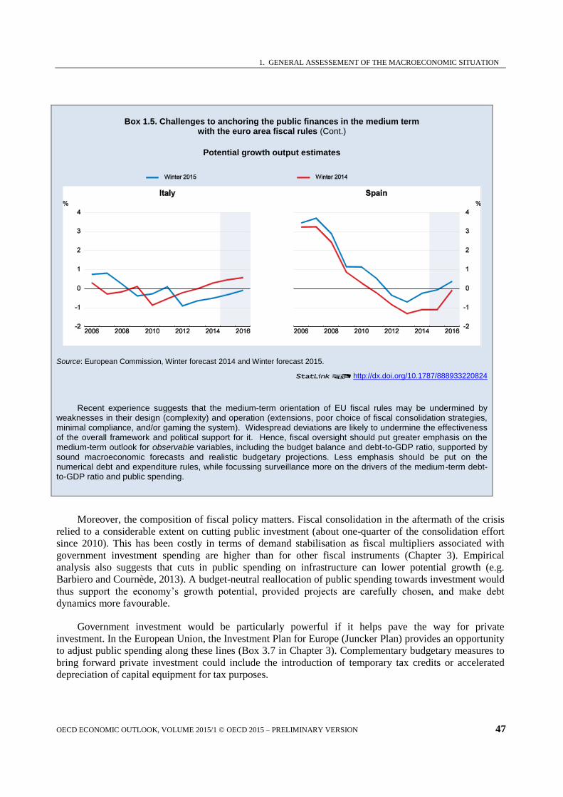
1. GENERAL ASSESSEMENT OF THE MACROECONOMIC SITUATION
OECD ECONOMIC OUTLOOK, VOLUME 2015/1 © OECD 2015 – PRELIMINARY VERSION 47
Box 1.5. Challenges to anchoring the public finances in the medium term with the euro area fiscal rules (Cont.)
Potential growth output estimates
Source: European Commission, Winter forecast 2014 and Winter forecast 2015.
12http://dx.doi.org/10.1787/888933220824
Recent experience suggests that the medium-term orientation of EU fiscal rules may be undermined by weaknesses in their design (complexity) and operation (extensions, poor choice of fiscal consolidation strategies, minimal compliance, and/or gaming the system). Widespread deviations are likely to undermine the effectiveness of the overall framework and political support for it. Hence, fiscal oversight should put greater emphasis on the medium-term outlook for observable variables, including the budget balance and debt-to-GDP ratio, supported by sound macroeconomic forecasts and realistic budgetary projections. Less emphasis should be put on the numerical debt and expenditure rules, while focussing surveillance more on the drivers of the medium-term debt-to-GDP ratio and public spending.
Moreover, the composition of fiscal policy matters. Fiscal consolidation in the aftermath of the crisis
relied to a considerable extent on cutting public investment (about one-quarter of the consolidation effort
since 2010). This has been costly in terms of demand stabilisation as fiscal multipliers associated with
government investment spending are higher than for other fiscal instruments (Chapter 3). Empirical
analysis also suggests that cuts in public spending on infrastructure can lower potential growth (e.g.
Barbiero and Cournède, 2013). A budget-neutral reallocation of public spending towards investment would
thus support the economy’s growth potential, provided projects are carefully chosen, and make debt
dynamics more favourable.
Government investment would be particularly powerful if it helps pave the way for private
investment. In the European Union, the Investment Plan for Europe (Juncker Plan) provides an opportunity
to adjust public spending along these lines (Box 3.7 in Chapter 3). Complementary budgetary measures to
bring forward private investment could include the introduction of temporary tax credits or accelerated
depreciation of capital equipment for tax purposes.

1. GENERAL ASSESSEMENT OF THE MACROECONOMIC SITUATION
48 OECD ECONOMIC OUTLOOK, VOLUME 2015/1 © OECD 2015 – PRELIMINARY VERSION
In addition, fiscal-structural policies should be adjusted to lessen pressures on public budgets and
strengthen output growth. Raising the effective retirement age can help to tackle the spending pressure that
ageing will create and would also support the productive potential of the economy. Also, OECD analysis
suggests that there is much scope for efficiency improvement in healthcare and education that would leave
the quality of services intact (Joumard et al., 2008; Sutherland et al., 2009).
Complete policy packages should integrate fiscal, monetary and demand-friendly structural
policies
Monetary and fiscal policy action should be supported by structural policy changes in an integrated,
rather than a piecemeal, approach. First, within structural policy, attention to labour and business settings is
important. For example, product market reforms undertaken in a strict labour environment tend to limit the
ability of new firms to hire the labour they need. Alternatively, labour market reforms undertaken within a
rigid business environment with large incumbent firms tend to force all adjustment onto labour. Overall,
structural policies can contribute substantially to fiscal sustainability and soften trade-offs between fiscal
consolidation, growth and equity objectives. But while such policy actions are often undertaken with a
view to boosting long-run growth from the supply side, their short-term effects on demand are less certain
and these must also be considered.
When pro-growth structural policies are introduced in normal times and with the support of other
macro policies, the empirical evidence generally points to greater short-term gains than losses. In bad
times, however, and especially when fiscal and monetary policies are not deployed to offset short-run
negative effects, the negative transitional dynamics associated with structural changes are not as easily
smoothed. In such a situation, structural policies that boost short-run demand should be prioritised. They
include policies that reduce entry barriers in sectors with pent-up demand, policies to reduce administrative
burdens on firms, and policies that boost aggregate demand directly such as public infrastructure
investment. Policies that improve confidence or reduce uncertainty over future economic conditions may
offer the biggest short-term impact as they can rapidly boost consumption and investment through wealth
effects and improved expectations. Examples include credible reforms to pension and health systems that
improve the sustainability of public finances, reducing the need for precautionary saving and creating fiscal
space for stimulus. A forthcoming OECD study on the short-term effects of structural reforms discusses
these issues in greater depth (Caldera Sanchez et al., 2015).

1. GENERAL ASSESSEMENT OF THE MACROECONOMIC SITUATION
OECD ECONOMIC OUTLOOK, VOLUME 2015/1 © OECD 2015 – PRELIMINARY VERSION 49
BIBLIOGRAPHY
Barbiero, O. and B. Cournède (2013), “New Econometric Estimates of Long-term Growth Effects of
Different Areas of Public Spending”, OECD Economics Department Working Papers, No. 1100,
OECD Publishing, Paris.
Barnes, S., D. Davidsson and Ł. Rawdanowicz (2012), “Europe’s New Fiscal Rules”, OECD Economics
Department Working Paper, No. 972, OECD Publishing, Paris.
Berg, T. (2015), “Quicksilver Markets”, OFR Brief Series, No. 15-02, Office of Financial Research,
March 17.
Bénétrix, A. S., P. R. Lane and J. C. Shambaugh (2014), “International Currency Exposures, Valuation
Effects and the Global Financial Crisis”, Mimeo.
Bernanke, B. S. and M. Gertler (1995), “Inside the Black Box: The Credit Channel of Monetary Policy
Transmission”, The Journal of Economic Perspectives, Vol. 9(4), pp. 27-48.
BIS (2014), “Market-making and Proprietary Trading: Industry Trends, Drivers and Policy Implications”,
CGFS Papers, No. 52, Bank for International Settlements.
BIS (2015), BIS Quarterly Review, March, Bank for International Settlements.
Caldera Sanchez, A., A. De Serres and N. Yashiro (2015), “The Short-Run Impact of Structural Reforms”,
OECD Economics Department Working Papers, OECD Publishing, Paris (forthcoming).
Carroll, C. D., J. Slacalek and K. Tokuoka (2014), “The Distribution of wealth and the MPC: implications
of new European data”, ECB Working Paper Series, No. 1648.
Cashin, P., K. Mohaddes and M. Raissi (2014), “The Macroeconomic Effects of El Niño”, Cambridge
Working Paper in Economics, No. 1418, University of Cambridge.
Çelik, S., G. Demirtaş and M. Isaksson (2015), “Corporate Bonds, Bondholders and Corporate
Governance”, OECD Corporate Governance Working Papers, No. 16, OECD Publishing, Paris.
Clayes, G., A. Leandro and A. Mandra (2015), “European Central Bank Quantitative Easing: The Detailed
Manual”, Bruegel Policy Contribution, Issue 2015/02, March.
ECB (2009), “Housing Finance in the Euro Area”, ECB Occasional Paper Series, No. 101.
ECB (2010), Structural Issues Report, June 2010, Chapter 3.
European Commission (2014), “Economic governance review - Report on the application of Regulations
(EU) n° 1173/2011, 1174/2011, 1175/2011, 1176/2011, 1177/2011, 472/2013 and 473/2013”,
COM(2014) 905 final.
Fall, F., D. Bloch, J-M. Fournier and P. Hoeller (2015), “Government Debt and Fiscal Frameworks”,
OECD Economic Policy Paper, forthcoming.

1. GENERAL ASSESSEMENT OF THE MACROECONOMIC SITUATION
50 OECD ECONOMIC OUTLOOK, VOLUME 2015/1 © OECD 2015 – PRELIMINARY VERSION
FRBNY (2014), “Domestic Open Market Operations during 2013”, Federal Reserve Bank of New York,
April.
Girouard, N. and C. André (2005), “Measuring Cyclically-adjusted Budget Balances for OECD
Countries”, OECD Economics Department Working Papers, No. 434, OECD Publishing, Paris.
Guichard, S., D. Haugh and D. Turner (2009), “Quantifying the Effect of Financial Conditions in the Euro
Area, Japan, United Kingdom and the United States”, OECD Economics Department Working
Papers, No. 677, OECD Publishing, Paris.
IEA (2015), “Medium-Term Oil Market Report 2015”, IEA, Paris.
IFF (2015), “March 2015 EM Portfolio Flows Tracker”, Institute of International Finance, 26 March.
IMF (2015a), “Private Investment: What’s the Holdup?”, World Economic Outlook, April.
IMF (2015b), Global Financial Stability Report, April.
Joumard, I., C. André, C. Nicq and O. Chatal (2008), “Health Status Determinants: Lifestyle, Environment,
Health Care Resources and Efficiency”, OECD Economics Department Working Papers, No. 627,
OECD Publishing, Paris.
Koske, I., I. Wanner, R. Bitetti and O. Barbiero (2015), “The 2013 update of the OECD's database on
product market regulation: Policy insights for OECD and non-OECD countries”, OECD Economics
Department Working Papers, No. 1200, OECD Publishing, Paris.
Kurosaki, T., Y. Kumano, K. Okabe and T. Nagano (2015), “Liquidity in JGB Markets: An Evaluation
from Transaction Data”, Bank of Japan Working Paper Series, No. 15-E-2.
Ministry of Land, Infrastructure, Transport and Tourism (2015), “平成26年度民間住宅ローンの実態に関する調査
結果報告書” (A Report of Survey on Private Housing Loans in Fiscal Year 2014), Housing Bureau,
Ministry of Land, Infrastructure, Transport and Tourism, Japanese Government.
Morin, M. and C. Schwellnus (2014), “An Update of the OECD International Trade Equations”, OECD
Economics Department Working Papers, No. 1129, OECD Publishing, Paris.
Mourre, G., C. Astarita and S. Princen (2014), “Adjusting the budget balance for the business cycle: the
EU methodology”, European Economy, Economic Papers, No. 536, European Commission.
OECD (2009), OECD Economic Outlook Interim Report, OECD Publishing, Paris.
OECD (2010), OECD Economic Surveys: Euro Area 2010, OECD Publishing
OECD (2013), Science, Technology and Industry Scoreboard 2013, OECD Publishing, Paris.
OECD (2014a), OECD Economic Outlook, Vol. 2014/1, OECD Publishing, Paris.
OECD (2014b), OECD Economic Outlook, Vol. 2014/2, OECD Publishing, Paris.
OECD (2015a), Economic Policy Reforms 2015: Going for Growth, OECD Publishing, Paris.
OECD (2015b), OECD Economic Survey. China, OECD Publishing, Paris.

1. GENERAL ASSESSEMENT OF THE MACROECONOMIC SITUATION
OECD ECONOMIC OUTLOOK, VOLUME 2015/1 © OECD 2015 – PRELIMINARY VERSION 51
OECD (2015c), OECD Business and Finance Outlook, OECD Publishing, Paris (forthcoming).
OECD (2015d), In It Together: Why Less Inequality Benefits All, OECD Publishing, Paris.
Ollivaud, P., E. Rusticelli and C. Schwellnus (2015), “The Changing Role of the Exchange Rate for
Macroeconomic Adjustment”, OECD Economics Department Working Papers, No. 1190, OECD
Publishing, Paris.
Ollivaud, P. and D. Turner (2015), “The effect of the global financial crisis on OECD potential output”,
OECD Journal: Economic Studies, Vol. 2014/1, OECD Publishing, Paris.
Rawdanowicz, Ł., R. Bouis and S. Watanabe (2013), “The Benefits and Costs of Highly Expansionary
Monetary Policy”, OECD Economics Department Working Papers, No. 1082, OECD Publishing,
Paris.
Rawdanowicz, Ł., R. Bouis, J. Brezillon, A. K. Christensen and K. Inaba (2014a), “Spillover Effects from
Exiting Highly Expansionary Monetary Policies”, OECD Economics Department Working Papers,
No. 1116, OECD Publishing, Paris.
Rawdanowicz, Ł., R. Bouis, J. Brezillon, K. Inaba and A. K. Christensen (2014b), “Secular Stagnation:
Evidence and Implications for Economic Policy”, OECD Economics Department Working Papers,
No. 1169, OECD Publishing, Paris.
Robertson, J. (2015), “What Seems to Be Holding Back Labor Productivity Growth, and Why It Matters”,
Atlanta Fed Macroblog, Federal Reserve Bank of Atlanta.
Sutherland, D., R. Price and F. Gonand (2009), “Improving public spending efficiency in primary and
secondary education,” OECD Journal: Economic Studies, Vol. 2009(1), pp. 1-30, OECD Publishing,
Paris.
Turner, D. and F. Spinelli (2013), “The Effect of Government Debt, External Debt and their Interaction on
OECD Interest Rates”, OECD Economics Department Working Papers, No. 1103, OECD
Publishing, Paris.
Wurzel, E., L. Willard and P. Ollivaud (2009), “Recent Oil Price Movements: Forces and Policy Issues“,
OECD Economics Department Working Papers, No. 737, OECD Publishing, Paris.

1. GENERAL ASSESSEMENT OF THE MACROECONOMIC SITUATION
52 OECD ECONOMIC OUTLOOK, VOLUME 2015/1 © OECD 2015 – PRELIMINARY VERSION
ANNEX 1.1: INDICATORS OF POTENTIAL FINANCIAL VULNERABILITIES
The following tables show the position of OECD and selected non-OECD countries on a number of
indicators that could reveal potential exposure to financial turbulence. The main focus of Table 1.A1 is on
domestic vulnerabilities of the OECD and BRIICS countries, that of Table 1.A2 on financial account
vulnerabilities of the OECD and non-OECD G20 countries.
Table 1.A1 presents indicators typically associated with financial vulnerabilities arising primarily
from the domestic economy in four broad categories: the real economy, the non-financial sector, the
financial sector and public finances (International Monetary Fund, 2012; European Commission, 2012).
Possible weaknesses in the real economy are captured by the difference between the potential and the
actual GDP growth rate, the difference between the actual unemployment rate and the natural rate of
unemployment (or NAIRU), the current account deficit and the evolution of relative unit labour costs.
Indicators of financial market excesses related to the non-financial sector are debt of households and non-
financial corporations and real house price growth. An aggregated ratio of core Tier-1 capital to total assets
(i.e. the leverage ratio) for selected banks in each country,1 non-performing loans, and financial
corporations’ debt are included to account for the direct risk exposure of the financial sector.
Vulnerabilities stemming from the public sector are quantified along three dimensions: government net
borrowing, gross government debt and the difference between 10-year real sovereign bond yields and the
potential real GDP growth rate. Higher values, with the exception of the leverage ratio, indicate a larger
vulnerability. Table 1.A1 also includes the current sovereign credit ratings issued by Standards and Poor’s.
Table 1.A2 displays financial-accounts-related risk factors for the OECD and non-OECD G20
countries to financial stability based on previous OECD empirical analysis (Ahrend and Goujard, 2012a,
2012b). The analysis shows that:
Greater (short-term) borrowing from external banks or a skew in external liabilities towards debt
increases the risk of a financial crisis substantially (external bank debt being defined as debt to a
foreign bank).
A larger share of FDI in gross external liabilities decreases chances of a financial crisis.
Shorter maturity of banks’ debt raises the crisis risk, mainly by increasing exposure to financial contagion.
The size of foreign reserve holdings reduces the probability of a crisis.
Total external assets (excluding reserves) or liabilities are found not to affect the risk for
countries with small and moderate levels of assets and liabilities. However, external assets reduce, and external liabilities increase the crisis risk when they are large.
1. The calculations of the country leverage ratios are based on over 1200 commercial banks, including 915 in
the United States, 197 in the OECD euro area countries, 23 in the United Kingdom, 11 in Canada and 7 in
Japan.

1. GENERAL ASSESSEMENT OF THE MACROECONOMIC SITUATION
OECD ECONOMIC OUTLOOK, VOLUME 2015/1 © OECD 2015 – PRELIMINARY VERSION 53
Table 1.A2 shows for each of the 8 selected indicators: i) the position of each country in 2014Q3 (or
the latest available) along various dimensions of its financial account structure, and ii) the country-specific
change, from 2007 to 2014Q3. For some of the variables, the numbers need to be interpreted with care as
the relevance of the variable may differ across countries. For example, the foreign currency reserves of the
United States are the lowest relative to GDP in the OECD area, but this does not signify a weakness as the
US dollar is a reserve currency, and the same applies to low currency reserves in individual euro area
countries.
BIBLIOGRAPHY
Ahrend, R., and A. Goujard (2012a), “International Capital Mobility and Financial Fragility – Part 1:
Drivers of Systemic Banking Crises: the Role of Bank-Balance-Sheet Contagion and Financial
Account Structure”, OECD Economics Department Working Papers, No. 902, OECD Publishing,
Paris.
Ahrend, R., and A. Goujard (2012b), “International Capital Mobility and Financial Fragility – Part 3: How
Do Structural Policies Affect Financial Crisis Risk? Evidence from Past Crises across OECD and
Emerging Economies”, OECD Economics Department Working Papers, No. 966, OECD
Publishing, Paris.
European Commission (2012), Alert Mechanism Report 2013, Brussels.
International Monetary Fund (2012), Global Financial Stability Report October 2012,Washington, DC.
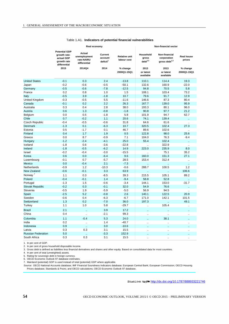
1. GENERAL ASSESSEMENT OF THE MACROECONOMIC SITUATION
54 OECD ECONOMIC OUTLOOK, VOLUME 2015/1 © OECD 2015 – PRELIMINARY VERSION
12http://dx.doi.org/10.1787/888933221746
Table 1.A1. Indicators of potential financial vulnerabilities
Real economy Non-financial sector
Potential GDP
growth rate-
actual GDP
growth rate
differential
Actual
unemployment
rate-NAIRU
differential
Current
account
deficit1
Relative unit
labour cost
Household
gross
debt2,3
Non-financial
corporation
gross debt1,3
Real house
prices
2015 2014Q4 2014 % change 2013 2013 % change
2000Q1-15Q1 or latest
available
or latest
available
2000Q1-15Q1
United States -0.1 0.3 2.4 -13.8 110.1 114.4 19.3
Japan -0.2 -0.6 -0.5 -50.1 132.6 160.9 -22.0
Germany -0.5 -0.6 -7.8 -12.5 94.8 70.5 5.8
France 0.2 0.8 1.0 1.5 108.1 103.4 73.2
Italy -0.5 3.9 -1.8 10.7 79.6 91.7 12.9
United Kingdom -0.3 -0.5 5.5 -11.6 146.6 87.3 80.4
Canada -0.1 0.2 2.2 26.3 167.7 139.0 95.9
Australia 0.3 0.4 2.8 38.0 193.3 80.1 96.0
Austria 0.6 1.3 -0.8 -1.8 90.8 97.7 21.2
Belgium 0.0 0.5 -1.8 5.8 101.9 94.7 62.7
Chile 0.7 -0.2 1.1 20.6 74.1 139.4 ..
Czech Republic -0.4 -0.5 -0.6 31.8 64.6 61.6 ..
Denmark -1.3 0.1 -6.3 10.7 320.5 102.4 27.3
Estonia 0.5 -1.7 0.1 46.7 89.6 102.6 ..
Finland 0.4 1.7 1.9 0.5 122.8 98.0 25.6
Greece 0.0 8.7 -0.9 7.1 104.0 76.3 -9.4
Hungary -1.2 -2.4 -4.1 25.0 55.4 102.4 ..
Iceland -1.8 0.6 -3.6 -22.8 .. 322.9 ..
Ireland -1.8 -0.5 -6.2 14.9 223.0 235.9 8.0
Israel -0.2 -0.4 -3.0 -15.5 .. 75.1 35.2
Korea 0.6 0.0 -6.4 9.6 160.0 151.3 27.1
Luxembourg -0.1 0.7 -5.7 28.5 153.4 312.4 ..
Mexico 0.0 -0.4 2.1 -7.3 .. .. ..
Netherlands -0.9 1.2 -10.3 -0.6 288.7 100.5 1.2
New Zealand -0.6 -0.1 3.3 63.9 .. .. 106.6
Norway 7
1.1 0.3 -8.5 39.3 215.5 105.1 89.2
Poland -0.4 -0.1 1.4 -9.4 58.8 52.8 ..
Portugal -1.3 1.5 -0.6 -3.4 144.1 153.0 -31.7
Slovak Republic -0.2 0.3 -0.1 32.0 54.9 76.6 ..
Slovenia -0.5 1.9 -5.9 -5.0 56.9 94.5 ..
Spain -2.5 5.2 -0.8 2.6 140.1 122.5 20.9
Sweden -0.6 0.4 -6.3 -6.7 171.0 142.1 101.5
Switzerland 1.3 0.2 -7.0 36.0 197.3 .. 49.1
Turkey 1.1 1.0 5.8 -29.7 .. 105.4 ..
Brazil 2.1 .. 3.9 17.2 .. .. ..
China 0.4 .. -2.1 99.3 .. .. ..
Colombia 1.1 -0.4 5.3 24.0 .. 38.1 ..
India 0.2 .. 1.4 -40.7 .. .. ..
Indonesia 0.9 .. 3.0 -10.6 .. .. ..
Latvia 0.3 0.3 3.1 15.5 .. .. ..
Russian Federation 5.0 .. -3.3 152.9 .. .. ..
South Africa 0.3 0.3 3.1 15.5 .. .. ..
1. In per cent of GDP.
2. In per cent of gross household disposable income.
3. Gross debt is defined as liabilities less financial derivatives and shares and other equity. Based on consolidated data for most countries.
4. In per cent of total (unweighted) assets.
5. Rating for sovereign debt in foreign currency.
6. OECD Economic Outlook 97 database estimates.
7. Mainland (potential) GDP is used instead of total (potential) GDP where applicable.
Source: OECD National Accounts database; IMF Financial Soundness Indicators database; European Central Bank; European Commission; OECD Housnig
Prices database; Standards & Poors; and OECD calculations; OECD Economic Outlook 97 database.
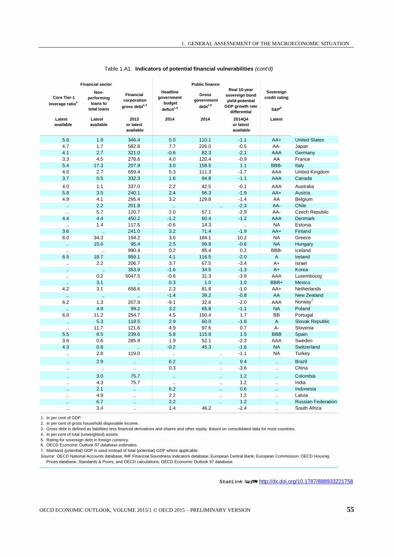
1. GENERAL ASSESSEMENT OF THE MACROECONOMIC SITUATION
OECD ECONOMIC OUTLOOK, VOLUME 2015/1 © OECD 2015 – PRELIMINARY VERSION 55
12http://dx.doi.org/10.1787/888933221758
Table 1.A1. Indicators of potential financial vulnerabilities (cont'd)
Financial sector Public finance
Core Tier-1
leverage ratio4
Non-
performing
loans to
total loans
Financial
corporation
gross debt1,3
Headline
government
budget
deficit1,6
Gross
government
debt1,6
Real 10-year
sovereign bond
yield-potential
GDP growth rate
differential
Sovereign
credit rating
S&P5
Latest Latest 2013 2014 2014 2014Q4 Latest
available available or latest
available
or latest
available
5.6 1.9 346.4 5.0 110.1 -1.1 AA+ United States
4.7 1.7 582.8 7.7 226.0 -0.5 AA- Japan
4.1 2.7 321.0 -0.6 82.3 -2.1 AAA Germany
3.3 4.5 278.6 4.0 120.4 -0.9 AA France
5.4 17.3 207.9 3.0 158.5 1.1 BBB- Italy
4.0 2.7 659.4 5.3 111.3 -1.7 AAA United Kingdom
3.7 0.5 332.3 1.6 94.8 -1.1 AAA Canada
4.0 1.1 337.0 2.2 42.5 -0.1 AAA Australia
5.8 3.5 240.1 2.4 96.3 -1.9 AA+ Austria
4.9 4.1 295.4 3.2 129.8 -1.4 AA Belgium
.. 2.2 201.8 .. .. -2.3 AA- Chile
.. 5.7 120.7 2.0 57.1 -2.9 AA- Czech Republic
4.4 4.4 450.2 -1.2 60.4 -1.2 AAA Denmark
.. 1.4 117.5 -0.6 14.3 .. NA Estonia
3.6 .. 241.0 3.2 71.4 -1.9 AA+ Finland
8.0 34.3 194.2 3.6 184.1 10.2 NA Greece
.. 15.6 95.4 2.5 99.8 -0.6 NA Hungary
.. .. 990.4 0.2 85.4 0.2 BBB- Iceland
6.5 18.7 959.1 4.1 116.5 -2.0 A Ireland
.. 2.2 206.7 3.7 67.5 -3.4 A+ Israel
.. .. 353.9 -1.6 34.5 -1.3 A+ Korea
.. 0.2 5047.5 -0.6 31.3 -3.9 AAA Luxembourg
.. 3.1 .. 0.3 1.0 1.0 BBB+ Mexico
4.2 3.1 658.6 2.3 81.8 -1.0 AA+ Netherlands
.. .. .. -1.4 39.2 -0.8 AA New Zealand
6.2 1.3 207.9 -9.1 32.6 -2.0 AAA Norway7
.. 4.9 99.2 3.2 65.8 -1.1 NA Poland
6.0 11.2 254.7 4.5 150.4 1.7 BB Portugal
.. 5.3 118.5 2.9 60.0 -1.8 A Slovak Republic
.. 11.7 121.6 4.9 97.6 0.7 A- Slovenia
5.5 8.5 239.6 5.8 115.8 1.5 BBB Spain
3.6 0.6 285.9 1.9 52.1 -2.3 AAA Sweden
4.3 0.8 .. -0.2 45.3 -1.6 NA Switzerland
.. 2.8 119.0 .. .. -1.1 NA Turkey
.. 2.9 .. 6.2 .. 9.4 .. Brazil
.. .. .. 0.3 .. -3.6 .. China
.. 3.0 75.7 .. .. 1.2 .. Colombia
.. 4.3 75.7 .. .. 1.2 .. India
.. 2.1 .. 6.2 .. 0.6 .. Indonesia
.. 4.9 .. 2.2 .. 1.2 .. Latvia
.. 6.7 .. 2.2 .. 1.2 .. Russian Federation
.. 3.4 .. 1.4 46.2 -2.4 .. South Africa
1. In per cent of GDP.
2. In per cent of gross household disposable income.
3. Gross debt is defined as liabilities less financial derivatives and shares and other equity. Based on consolidated data for most countries.
4. In per cent of total (unweighted) assets.
5. Rating for sovereign debt in foreign currency.
6. OECD Economic Outlook 97 database estimates.
7. Mainland (potential) GDP is used instead of total (potential) GDP where applicable.
Source: OECD National Accounts database; IMF Financial Soundness Indicators database; European Central Bank; European Commission; OECD Housnig
Prices database; Standards & Poors; and OECD calculations; OECD Economic Outlook 97 database.
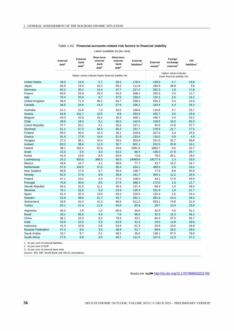
1. GENERAL ASSESSEMENT OF THE MACROECONOMIC SITUATION
56 OECD ECONOMIC OUTLOOK, VOLUME 2015/1 © OECD 2015 – PRELIMINARY VERSION
12http://dx.doi.org/10.1787/888933221760
Table 1.A2. Financial-accounts-related risk factors to financial stability
Latest available (in per cent)
External
debt1
External
bank
debt2
Short-term
external
bank
debt2
Short-term
external
bank
debt3
External
liabilities2
External
assets2
Foreign
exchange
reserves2
FDI
liabilities1
Higher values indicate higher financial stability riskHigher values indicate
lower financial stability risk
United States 49.3 14.6 5.7 39.3 178.5 139.5 0.7 19.8
Japan 56.9 19.3 16.3 84.2 111.8 184.9 28.9 3.6
Germany 60.2 30.2 14.4 47.7 217.4 252.3 1.8 17.8
France 60.0 53.9 29.3 54.3 308.2 292.3 2.0 12.7
Italy 70.4 25.9 9.7 37.5 159.0 132.1 2.6 15.2
United Kingdom 56.0 71.3 46.2 64.7 539.4 534.2 3.4 10.5
Canada 48.5 24.8 14.3 57.6 156.2 163.4 4.3 34.2
Australia 51.1 21.8 7.3 33.5 168.6 116.8 3.7 25.7
Austria 64.8 141.7 12.5 8.8 253.3 255.7 3.5 29.0
Belgium 40.3 42.8 19.4 45.3 405.1 446.7 3.4 53.2
Chile 28.9 18.0 8.1 45.0 142.6 128.5 16.0 62.3
Czech Republic 37.7 20.1 5.1 25.5 127.1 92.9 27.8 57.7
Denmark 61.1 57.3 34.5 60.2 237.7 276.9 21.7 17.5
Finland 59.3 45.0 15.3 34.1 318.8 327.3 3.4 15.6
Greece 91.9 27.8 14.4 51.9 233.0 116.0 0.9 4.0
Hungary 27.2 35.1 10.4 29.5 303.9 231.5 32.7 69.8
Iceland 83.2 38.6 11.9 30.7 601.1 242.0 23.9 16.1
Ireland 38.1 152.2 61.8 40.6 1961.6 1862.7 0.6 16.7
Israel 32.3 5.6 3.0 53.2 89.4 106.3 27.8 35.7
Korea 41.0 13.6 8.5 62.6 72.6 78.5 26.1 18.2
Luxembourg 25.2 920.6 368.3 40.0 14069.8 14277.4 1.3 33.0
Mexico 49.6 10.7 4.1 38.6 77.7 43.7 15.2 34.7
Netherlands 57.0 104.5 37.0 35.4 434.1 480.6 2.6 19.2
New Zealand 55.8 17.0 6.7 39.4 136.7 77.6 8.9 30.9
Norway 62.5 27.6 9.9 35.8 181.7 305.1 11.2 26.9
Poland 47.1 23.2 6.3 27.0 108.5 43.1 17.8 43.9
Portugal 70.6 30.6 8.5 27.6 288.3 172.0 1.5 21.7
Slovak Republic 50.2 31.5 11.1 35.4 137.4 69.3 1.0 49.0
Slovenia 76.1 22.6 5.3 23.3 145.3 101.9 1.9 21.7
Spain 61.4 32.3 13.0 40.2 229.5 132.4 2.5 24.4
Sweden 52.9 48.6 21.7 44.7 291.1 281.9 10.4 28.2
Switzerland 33.5 61.5 41.0 66.6 511.3 633.1 74.8 31.9
Turkey 65.1 21.4 11.6 54.0 82.4 28.7 13.4 25.6
Argentina 44.4 2.5 1.5 60.5 34.6 42.0 4.5 51.1
Brazil 33.1 65.5 4.6 7.0 66.0 32.3 15.3 46.2
China 36.1 10.3 8.2 79.3 43.1 60.4 37.5 56.7
India 53.9 10.2 5.5 53.9 41.6 24.0 14.8 29.6
Indonesia 41.3 10.8 5.8 53.9 61.3 20.6 10.6 44.8
Russian Federation 47.4 8.4 3.3 38.8 51.7 69.6 18.2 39.0
Saudi Arabia 15.7 8.7 5.1 58.2 35.6 138.1 97.5 78.6
South Africa 27.0 8.8 3.5 40.1 111.5 107.5 12.3 37.2
1. As per cent of external liabilities.
2. As per cent of GDP.
3. As per cent of external bank debt.
Source : BIS; IMF; World Bank and OECD calculations.

1. GENERAL ASSESSEMENT OF THE MACROECONOMIC SITUATION
OECD ECONOMIC OUTLOOK, VOLUME 2015/1 © OECD 2015 – PRELIMINARY VERSION 57
12http://dx.doi.org/10.1787/888933221776
Table 1.A2. Financial-accounts-related risk factors to financial stability (cont'd)
Change from 2007 (in percentage points)
External
debt1
External
bank
debt2
Short-term
external
bank
debt2
Short-term
external
bank
debt3
External
liabilities2
External
assets2
Foreign
exchange
reserves2
FDI
liabilities1
Positive values indicate an increase in the financial stability riskPositive values indicate a
decrease in the financial stability risk
-5.8 -5.9 -3.0 -3.5 24.1 -6.0 0.2 1.0 United States
1.9 6.3 7.2 14.4 38.2 60.4 6.7 -0.8 Japan
-7.5 -20.0 -13.5 -7.8 11.8 17.7 0.3 -0.9 Germany
0.0 -13.5 -14.3 -10.4 5.8 -0.6 0.0 -0.4 France
-1.2 -25.4 -8.7 1.6 0.0 0.1 1.0 0.4 Italy
-8.8 -44.8 -40.6 -10.0 -30.2 -12.5 1.6 2.9 United Kingdom
13.8 1.4 -0.4 -5.4 -13.4 6.9 1.1 -12.3 Canada
2.3 -10.1 -4.8 -4.6 -5.4 7.5 0.8 0.2 Australia
1.3 69.6 -14.3 -28.3 -70.8 -57.2 0.4 2.4 Austria
-21.6 -72.1 -69.4 -32.0 -111.6 -101.8 1.0 19.2 Belgium
-3.6 -0.2 -1.5 -7.6 41.2 26.6 5.6 1.7 Chile
4.1 -2.5 -3.7 -13.6 16.1 26.4 8.2 0.2 Czech Republic
-6.7 -13.8 -2.3 8.4 -14.4 31.2 10.8 -3.8 Denmark
20.0 5.0 2.7 2.5 35.9 75.6 0.4 -3.3 Finland
16.5 -31.3 -2.5 23.2 33.1 22.1 0.6 -4.9 Greece
-4.3 -28.8 -7.5 1.6 -8.9 18.6 14.5 5.7 Hungary
3.8 -252.5 -114.1 -12.5 -133.9 -369.2 10.2 1.1 Iceland
-15.4 -117.3 -88.9 -15.3 534.8 456.7 0.3 2.2 Ireland
-12.5 -2.9 -0.9 7.2 -30.0 -12.6 10.7 10.6 Israel
-1.8 -3.3 -1.9 0.8 -0.1 23.3 1.8 2.6 Korea
-3.8 -236.9 -139.7 -3.9 703.7 790.7 1.0 8.5 Luxembourg
15.9 2.8 1.7 8.3 9.3 12.6 6.5 -9.0 Mexico
-1.8 -32.3 -31.0 -14.3 -61.3 -8.2 1.1 -1.7 Netherlands
-2.6 -8.5 -6.2 -11.4 -43.7 -17.2 -5.1 -1.6 New Zealand
-1.5 -33.9 -30.6 -30.0 -43.3 17.9 -5.6 7.1 Norway
1.8 -1.2 0.2 2.1 2.6 -0.2 1.4 -2.3 Poland
0.8 -44.4 -19.4 -9.5 -9.7 -28.4 0.6 3.0 Portugal
9.1 -0.3 -1.1 -3.2 17.9 10.1 -25.2 -8.4 Slovak Republic
4.5 -25.8 -7.8 -3.7 2.4 -15.8 -0.3 -3.3 Slovenia
-2.6 -27.2 -6.0 8.3 -6.3 -15.8 1.6 4.0 Spain
3.2 -5.5 -10.7 -15.2 9.2 1.6 4.5 -3.7 Sweden
-16.1 -111.0 -84.3 -6.0 -69.8 -100.6 64.6 11.0 Switzerland
10.4 2.5 3.2 9.8 -0.8 -0.6 0.8 -6.5 Turkey
-9.7 -4.3 -1.9 10.2 -22.9 -26.8 -10.4 11.8 Argentina
6.9 57.8 1.0 -40.2 -7.8 1.3 0.8 12.4 Brazil
3.9 4.3 4.9 24.1 4.6 -15.5 -10.5 -0.6 China
4.3 -1.2 -0.4 1.9 1.0 -9.2 -11.6 3.9 India
-11.9 0.2 0.2 0.8 -0.1 -2.7 -1.8 13.1 Indonesia
11.8 -5.6 -3.4 -8.9 -57.9 -26.7 -23.0 -0.5 Russian Federation
-20.7 -0.3 -0.6 -4.2 5.0 7.0 16.6 15.0 Saudi Arabia
7.3 -2.7 -1.7 -5.0 -2.3 27.3 1.7 -4.2 South Africa
1. As per cent of external liabilities.
2. As per cent of GDP.
3. As per cent of external bank debt.
Source : BIS; IMF; World Bank and OECD calculations.