chapter 1: configurations and...

Chapter 1: Configurations and Velocities

Ross Hatton and Howie Choset

Degrees of Freedom

•  I used to like relative motion between rigid bodies

•  I used to like relative motion from a frame •  Lets go with number of independent ways

a system can move – Translation – Rotation – Bending at joint

Configuration Space

•  configuration, denoted q, is an arrangement of degrees of freedom that uniquely defines the location in the world of each point on the system

•  Configuration space Q is the set of al q •  Dim(Q) = #DOF

Non-rotational 1 DOF Qs

Not linear but related

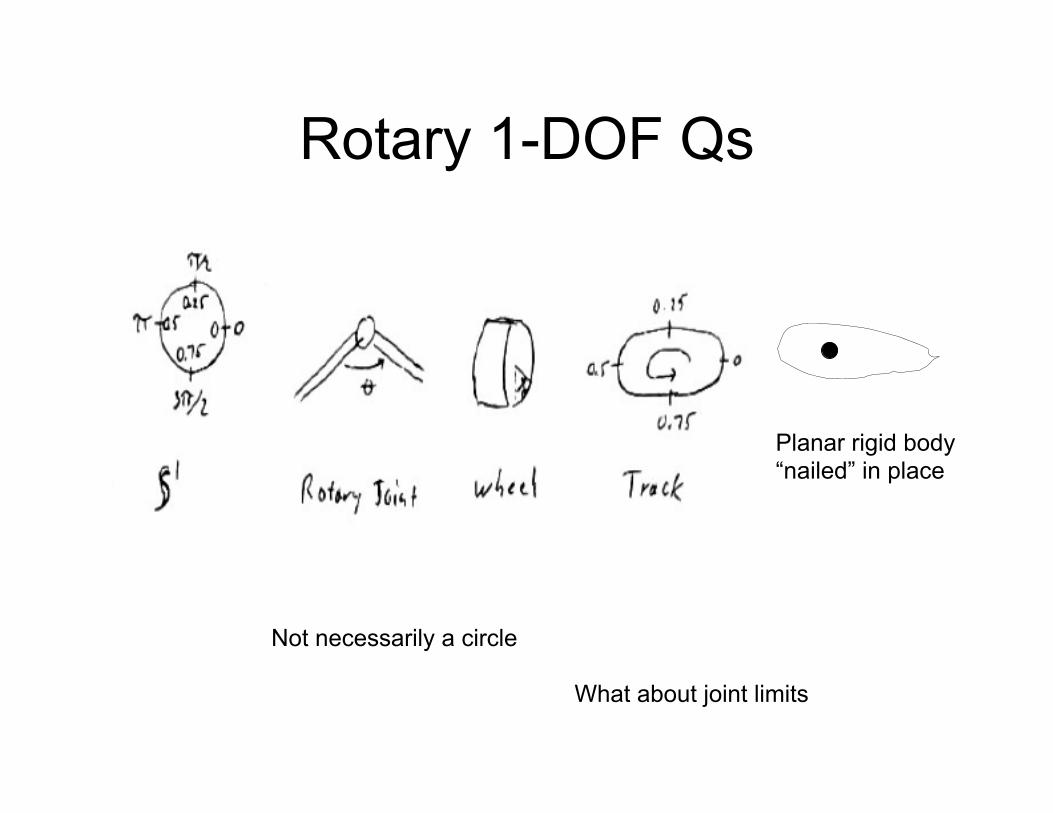
Rotary 1-DOF Qs

Not necessarily a circle

Planar rigid body “nailed” in place

What about joint limits

Manifold •  manifold is a space that is locally

like a Euclidean space, but may have a more complicated global structure

•  described by the an atlas of charts corresponding to the manifold –  chart is a region of Euclidean

space that maps to a region of the manifold

–  atlas is a set of overlapping charts that collectively describe the entirety of the manifold

Manifold: Charts •  charts inherently parameterize a

space by assigning points in Euclidean space

•  multi-chart atlases is to “paper over” singularities: latitude-longitude map is singular at the poles, and so must be combined with additional maps

•  Overlap maps: At the overlap,

between charts, there is naturally a mapping from each chart into the manifold, then back out into the other chart. These composite functions are the transition maps between charts, describing how to translate coordinates on one chart to coordinates on a second chart

Ck-differentiable Manifolds 1.  The mappings from the charts to the manifolds must each be k-times

differentiable, i.e., they must be Ck-diffeomorphisms. 2. All overlap maps for charts in the atlas must be Ck-diffeomorphisms

When k=∞, then the manifold is a smooth or differential manifold

Homeo- and Diffeomorphisms •  Recall mappings:

–  φ: S → T –  If each elements of φ goes to a unique T, φ is injective (or 1-1) –  If each element of T has a corresponding preimage in S, then φ

is surjective (or onto). –  If φ is surjective and injective, then it is bijective (in which case

an inverse, φ-1 exists). –  φ is smooth if derivatives of all orders exist (we say φ is C∞)

•  If φ: S → T is a bijection, and both φ and φ-1 are continuous, φ is a homeomorphism; if such a φ exists, S and T are homeomorphic.

•  If homeomorphism where both φ and φ-1 are smooth is a diffeomorphism.

Homeo/Diffeo-morphisms Homeomorphism Diffeomorphism Ck-

Diffeomorphism f Continuous, C0 Smooth, C∞ Ck differentiable f-1 Continuous, C0 Smooth, C∞ Ck differentiable f bijective bijective bijective

Surjective: Every point in the range is a function of at least one point in the domain many to one mapping, e.g., sine is surjective onto [-1,1] Injective: One to one, e.g., every point in the domain maps to a unique point in the range Bijective: BOTH

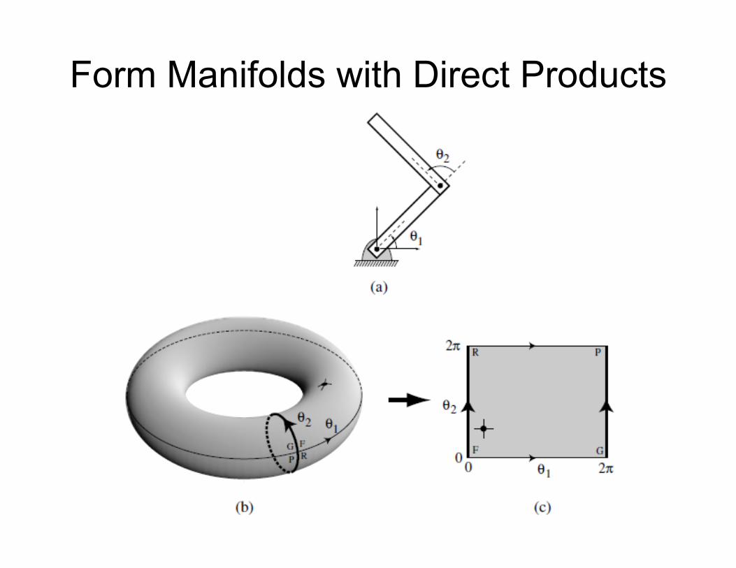
Form Manifolds with Direct Products

Form Manifolds with Direct Products Products

The Sphere

Similarities Differences

Lie Groups: Manifold + Group

•  Motivation – Perform algebraic operations on configurations, say

add or subtract – Rigid body motion is nicely described by Lie Groups – Another?

•  What’s a group? •  Examples of groups •  Same manifold, different group

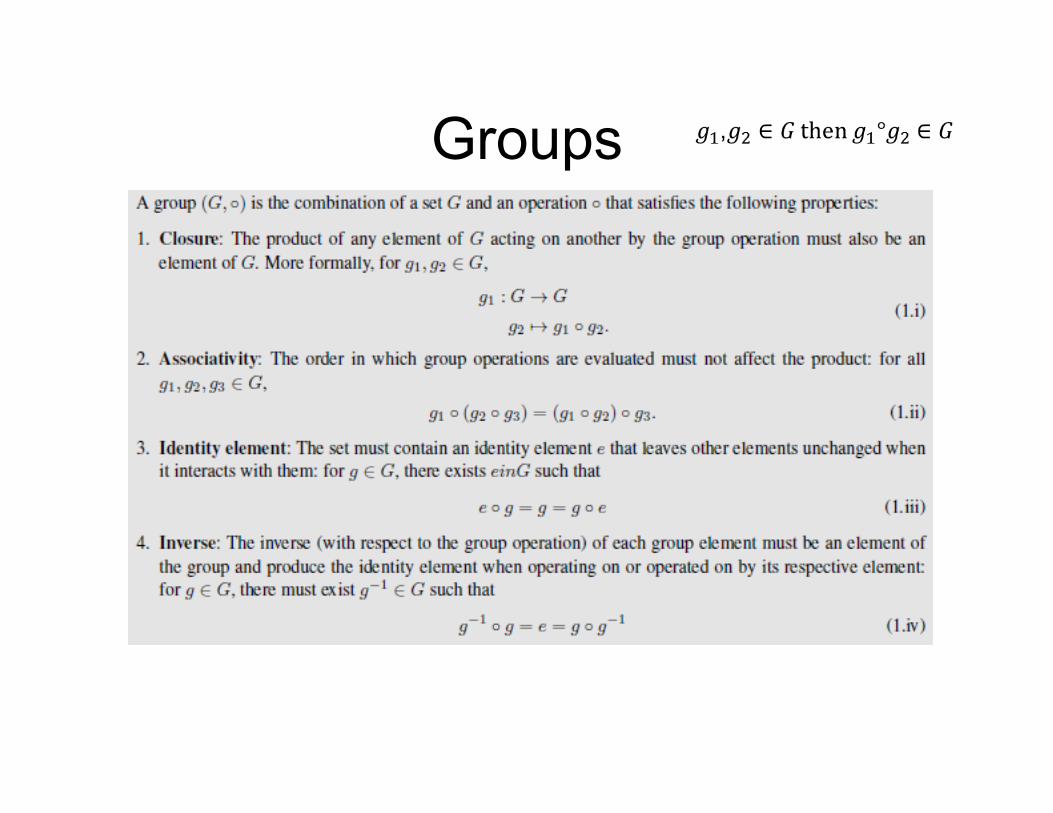
Groups

Left and Right Actions •  Left Action •  Right Action

•  Abelian groups (additive)

•  Most groups are not abelian, ie matrix multiplication does not commute

ghgLh =

hggRh =

gRhghgghghgL hh ==+=+==

Examples of Groups

?)(\)()(}1)det(|)({)(}1)det(|{)(

}0)det(|{),(),( 1

nSOnOnNSSOAnOAnSOARAnO

ARAxR

R

nn

nn

=

=∈=

±=∈=

≠∈

+

×

×

+

Combinations of lines and circles created via the direct product naturally inherit the group structures of their component spaces, with (modular) addition acting independently along each degree of freedom.

One Manifold, Many Groups

Consider θ is magnitude of rotation )),2(( ×SO

)mod,( 1 kS +

matrices are smooth, cyclic, and unique with respect to theta, so homeomorphic to a circle

Consider modular arithmetic Mod k for k = 2π, it is the common mod + What meaning does SO(2) have? How do they generalize? Not the same way

Rigid Body Configurations •  An object that does not deform in response to external

forces •  Set of points with fixed interpoint distances and relative

orientation •  Movable reference point and all points are fixed with

respect to this frame (infinitely large bodies)

Choices of body frame? Origin: Center of mass What about orientation?

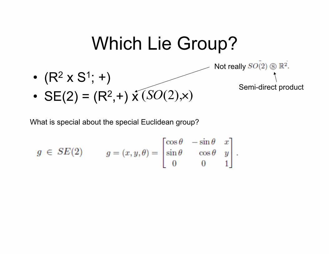
Which Lie Group?

•  (R2 x S1; +) •  SE(2) = (R2,+) x

Not really

What is special about the special Euclidean group?

Semi-direct product )),2(( ×SO

Direct/Semi- Product with Groups

Interpretations of SE(2)

•  1. the position and orientation of rigid bodies •  2. the position and orientation of coordinate

frames •  3. actions that move a rigid body or coordinate

frame with respect to a fixed coordinate frame •  4. actions that take a point in one coordinate

frame, and find the equivalent point in a second coordinate frame.

the position and orientation of a rigid object inherently identifies a body coordinate frame aligned with the object’s longitudinal and lateral axes, and vice versa.

Interpretations of SE(2)

•  1. the position and orientation of rigid bodies •  2. the position and orientation of coordinate

frames •  3. actions that move a rigid body or coordinate

frame with respect to a fixed coordinate frame •  4. actions that take a point in one coordinate

frame, and find the equivalent point in a second coordinate frame.

Actions make these groups, and in particular Lie groups

Identity Element in SE(2)

⎥⎥⎥

⎦

⎤

⎢⎢⎢

⎣

⎡

==

100010001

)0,0,0(I

When both left and right actions return the identity element

Right Action in SE(2)

starting at position g and moving by h relative to this starting position or finding the global position of the point at h relative to g,

Left Action in SE(2)

1.  g as the (x; y, θ) coordinates of a rigid body, and 2.  h as an action that transforms g by first rotating the body

around the origin by β, 3.  then translating it by (u; v),

OR - (absolute) location of the system as if g were defined with respect to h rather than the origin.

SE(2) vs. (R2 x S1,+) (right action)

Symmetries, Coming soon

Unify Frames and Points

Tangent Spaces

Tangent Spaces

Tangent spaces are “flat” spaces whose elements are vectors based at point

Two Dimensional Tan Space

Notation and Velocity

QTqQq q∈∈ havecan we, aFor

configuration

configuration space

velocity

tangent space

State and Bundles

( )qqx ,= ),( QTqTQQq

q∈

=

State Tangent Bundle

Vector Fields Vector field assigns a vector to each point on a manifold

),(::

vqqXTQQX

→

vqXQTQX q

:

: →

Examples: gradient vector field potential vector field constant vector field

For

On Lie Groups, left and right invariant vector fields

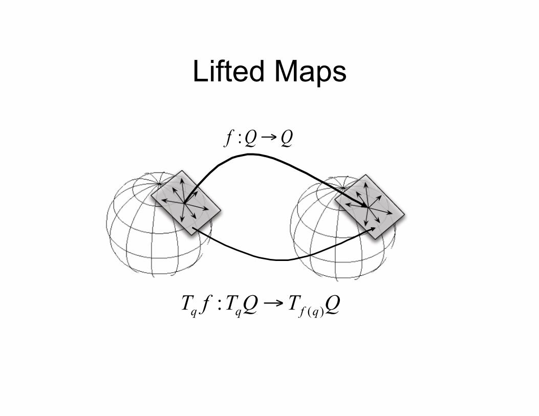
Lifted Maps

( ):q q f qT f T Q T Q→

QQf →:

Equivalence •  Sometimes there is a structure that allows us to

consider pairs of vectors in different tangent spaces as equivalent

•  When this structure is present, the lifted map

between these two spaces identifies these two vectors

•  For Lie groups, the group provides this structure,

e.g., left lifted map, right lifted map

Left Lifted Maps (on Lie Groups)

Bonus question: what is wrong with this figure?

Lh : G → G

g �→ hg

TgLh : TgG → ThgG

g �→ TgLhg

Left Lifted Maps (on Additive Groups)

On additive groups, equivalent vectors all have the same components, Which means we care carefeely and carelessly add vectors wherever we want.

Left Lifted Maps (on Lie Groups)

Equivalent vectors are scaled in proportion to the group position This calculation illustrates that equivalent vectors on multiplicative groups are based on the proportional rate of change

Review of Notation

More Complex Use of Lifted Actions: Body Velocity

World Velocity Body Velocity

rotating the translational component by -θ (equivalent to rotating the reference frame by θ) and leaving the rotational component unchanged,

Left Lifted Action on SE(2) •  Gain greater insight into rigid body motion and apply some powerful

mathematical tools to these systems •  Let g = (x,y,θ), h = (u,v,β)

-Looks similar to matrix on previous slide -Preserves body velocity (magnitude of translation remains fixed) -For any Lh that rotates by β, the lifted action rotates the translational component of the velocity vector by β

h = g-1, lifted action gives body velocity

From h = g-1 to Lie Algebra

Physically, body velocity is velocity vector in body frame Algebraically, body velocity is left-equivalent velocity at the origin. Because moving to the origin is the same as moving the origin to you, this is OK.

TeG is the Lie algebra. One can do a lot in a Lie algebra

Right Lifted Action on SE(2) (was a cross product)

The velocity of two rigid frames on the same rigid body given we know the velocity of one of them

Figure on the right considers a frame attached to the body and over the origin

l = (u, v)

Right Lifted Action on SE(2)

•  What does Rgh in SE(2) do? •  finds the frame at position and orientation

h with respect to g.

Same relationship as before!

Spatial Velocity: h = g-1

The velocity a point on the rigid body that passes through the origin Note: such a point may be imaginary, as one would imagine infinitely large rigid bodies

Adjoint

Review of SE(2) Left actions move elements

Right actions concern relative positions of elements

Left lifted actions preserve body velocity - Two frames with left-equivalent velocity are each moving the same with respect to themselves

Right lifted actions preserve spatial velocity -Two frames with right-equivalent velocity are moving as if rigidly attached (i.e., they remain a constant transformation away from each other as their trajectories evolve)

Where does this equivalence come from?

Velocity means different things when talking about addition and multiplication. We can understand this difference better if we think about Multiplicative Calculus

Continuous Discrete

Addition

�

Integral

�

Sum

Multiplication �Product-integral

�

Product

Multiplicative Calculus In familiar Newton-Leibniz calculus, an integral is difference between the value of a function at two points, and is calculated as the cumulative sum of many small changes to the function:

F (b)− F (a) =

� b

au(x) dx = lim

n→∞

n�

k=1

u(xk) ∆x

F(b)

F(a)=

b

�a

(I + v(x) dx) = limn→∞

n�

k=1

(I + v(xk) ∆x)

This makes sense on additive groups, where sums sums and differences are well-defined. On multiplicative groups, however, we don’t have these operations. Instead, we have products and quotients. If generalize the notion of an integral to be the cumulative composition of small group elements, then we should be using Volterra’s multiplicative calculus, in which integrals are quotients built of small multiplications:

Multiplicative Calculus: Derivatives In additive calculus, the derivative of a function is based on the difference between function values at consecutive points:

In multiplicative calculus, the same idea holds, except that we take the quotient of function values, not their difference:

u(x) = lim∆x→0

F (x+∆x)− F (x)

∆x

v(x) = lim∆x→0

�F (x+∆x)/F (x)

�− I

∆x

Note that we subtract out the identity term, so that v is a small deviation from the identity element.

Derivatives on Multiplicative Lie Groups Two velocities to consider: • Velocity through the manifold (i.e. rate of change of the parameters) – Additive • Group velocity – Multiplicative When we talk about equivalent velocities, we are typically asking “For a given group velocity, what is the parameter velocity at different configurations? First step to find this: Transform multiplicative velocity into additive time derivative

ßif this quantity is equal for two configuration/velocity pairs, the system velocity is equivalent under the group action

v(t) = lim∆t→0

�g(t+∆t)/g(t)

�− I

∆t

= lim∆t→0

g−1(t)�g(t+∆t)− g(t)

�

∆t

= g−1(t) lim∆t→0

�g(t+∆t)− g(t)

�

∆t

= g−1(t)dg

dt(t)

Derivatives on Multiplicative Lie Groups

How does this relate to the lifted action? So far, we have a means of converting between group velocities and the time rate of change of the group parameter:

continued

v(t) = g−1(t)dg

dt(t)

Earlier, we said that two velocities were equivalent according to the group if they were related by the lifted form of the group action:

g ∈ TgG ≡ (TgLhg) ∈ ThgG

Are these notions the same?

Derivatives on Multiplicative Lie Groups

Yes!

This looks very similar to our test for equivalence of multiplicative velocity:

continued

Two vectors are equivalent (according to the lifted action) if and only if they share an equivalent vector at the group identity:

g ∈ TgG ≡ h ∈ ThGiff

TgLg−1 g = ThLh−1 h = ξ

dg

dt≡ dh

dtiff g−1 dg

dt= h−1 dh

dt= v

And is in fact the same test for equivalence, modulo operations to convert between n-tuple and matrix representations of groups

Geodesics

“Straight lines” through a space Often also the locally-shortest paths

Geodesics on SE(2)

Geodesics on SE(2) are trajectories with constant body or spatial velocity

Straight lines if no rotaton, helices (that project to circles on xy) if rotation present

Note that even though the xy magnitude of right-equivalent velocities is not constant over the whole space, it is constant along a geodesic, and that the geodesics are the same for left and right actions – intuitively, if all the factors are the same, it doesn’t matter if you multiply from left or right

SE(2) vs. (R2 x S1,+), revisited

Exponential Map

•  Unit-time paths along geodesics •  Equivalently, either flow along a left- or

right-invariant field for 1 unit of time, or (on a multiplicative group) take a product-integral for one unit of time with constant group velocity.

Exponential maps and ex

•  How does this relate to standard notion of exponential as exp(x) = ex? (note that e here is not the same as group-identity e) – – exp(x) on multiplicative group is unit-time

path along always-accelerating (or decelerating) trajectory.

Exponential maps and ex continued


– – over any interval, ratio of start and end values will always be the same – this is the same basic definition

–  for a function kx – – e is by definition the value of exp(1) on the

multiplicative group (unit flow along the exponentia ltrajectory starting with a slope of 1)


– – once we have e1 = exp(1), everything else follows. For example, increasing the magnitude of the argument just pushes the result further along the curve, and we then have identities like

– exp(2)/ exp(1) = exp(1)/ exp(0) → exp(2) = e2

Exponential maps and power series

1.6 Geodesics 25

Figure 1.19 Constant-velocity paths on (R2 × S1,+) (left) and SE(2) (right)

1.6.4 Exponential Map• Exponential map of a velocity is ending point of a unit-time flow along the corresponding geodesic.• Relates (at least locally) structure of the manifold or group to tangent space at the identity.• How does this relate to standard notion of exponential as exp(x) = ex? (note that e here is not the same as

group-identity e)– exp(x) on multiplicative group is unit-time path along always-accelerating (or decelerating) trajectory.– over any interval, ratio of start and end values will always be the same – this is the same basic definition

for a function kx

– e is by definition the value of exp(1) on the multiplicative group (unit flow along the exponential trajectorystarting with a slope of 1)

– once we have e1 = exp 1, everything else follows. For example, increasing the magnitude of the argumentjust pushes the result further along the curve, and we then have identities like

exp(2)/ exp(1) = exp(1)/ exp(0) → exp(2) = e2 (1.48)

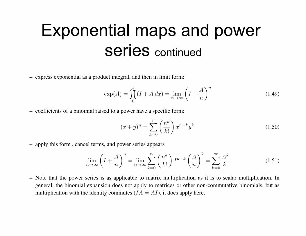
• How does this relate to power series expression for an exponential, exp(A) =�∞

k=0(Ak/k!)?

– express exponential as a product integral, and then in limit form:

exp(A) =1

�0

(I +A dx) = limn→∞

�I +

A

n

�n

(1.49)

– coefficients of a binomial raised to a power have a specific form:

(x+ y)n =n�

k=0

�nk

k!

�xn−kyk (1.50)

– apply this form, cancel terms, and power series appears

limn→∞

�I +

A

n

�n

= limn→∞

n�

k=0

�nk

k!

�In−k

�A

n

�k

=∞�

k=0

Ak

k!(1.51)

– Note that the power series is as applicable to matrix multiplication as it is to scalar multiplication.• Exponential maps on Lie groups are compatible either as flows along the left- and right-invariant fields, or as

exponentiations of the corresponding group velocity.• Useful relationships between group and body velocities (based on relationship between group and parameter

velocities, evaluated at the identity):

vR = g−1 dgmatrix

dgparamdgparam

dt

��g=e

(1.52)

Probably, someone at some point has told you that exp(A) can be found by a power series (or Taylor expansion),

How does this relate to our definition of an exponential?

Exponential maps and power series continued

1.6 Geodesics 25

Figure 1.19 Constant-velocity paths on (R2 × S1,+) (left) and SE(2) (right)

1.6.4 Exponential Map

• Exponential map of a velocity is ending point of a unit-time flow along the corresponding geodesic.

• Relates (at least locally) structure of the manifold or group to tangent space at the identity.

• How does this relate to standard notion of exponential as exp(x) = ex? (note that e here is not the same as

group-identity e)

– exp(x) on multiplicative group is unit-time path along always-accelerating (or decelerating) trajectory.

– over any interval, ratio of start and end values will always be the same – this is the same basic definition

for a function kx

– e is by definition the value of exp(1) on the multiplicative group (unit flow along the exponential trajectory

starting with a slope of 1)

– once we have e1 = exp 1, everything else follows. For example, increasing the magnitude of the argument

just pushes the result further along the curve, and we then have identities like

exp(2)/ exp(1) = exp(1)/ exp(0) → exp(2) = e2 (1.48)

• How does this relate to power series expression for an exponential, exp(A) =�∞

k=0(Ak/k!)?

– express exponential as a product integral, and then in limit form:

exp(A) =1

�0

(I +A dx) = limn→∞

�I +

A

n

�n

(1.49)

– coefficients of a binomial raised to a power have a specific form:

(x+ y)n =n�

k=0

�nk

k!

�xn−kyk (1.50)

– apply this form , cancel terms, and power series appears

limn→∞

�I +

A

n

�n

= limn→∞

n�

k=0

�nk

k!

�In−k

�A

n

�k

=∞�

k=0

Ak

k!(1.51)

– Note that the power series is as applicable to matrix multiplication as it is to scalar multiplication. In

general, the binomial expansion does not apply to matrices or other non-commutative binomials, but as

multiplication with the identity commutes (IA = AI), it does apply here.

• Exponential maps on Lie groups are compatible either as flows along the left- and right-invariant fields, or as

exponentiations of the corresponding group velocity.

Exponential maps and power series continued

Invariant-field exponentiation is equivalent to group velocity exponentiation

exp

0 −ξθ ξxξθ 0 ξy0 0 0

≡ exp(ξ)

SE(2) multiplicative velocity as a function of the body velocity parameters

Reference and Coordinate Frames

20 Configurations and Velocities

Frames

The kinematics and mechanics approaches discussed in this book are heavily based on the interactions offrames. In such discussions, it is important to recognize two distinctions that are sometimes overlooked: thedifference between a reference frame and a coordinate frame, and the difference between the moving andinstantaneous body frames of a system.

Reference frames define a sense of relative motion with respect to an “observer”. Whenever we describe apoint as moving with a certain velocity, this is implicitly with respect to a chosen reference frame, such as astationary inertial frame or a moving reference frame associated with a rigid body.

Coordinate frames parameterize reference frames, providing them with origins, scales, and orientations.Multiple coordinate frames may be associated with a single reference frame. For example, consider a pointmoving on this page, with a velocity vector as illustrated below. We can measure its position and velocitywith respect to either coordinate frame shown, but the point and its velocity vector have a fundamentalexistence in the reference frame of the page, independent of the choice of parameterization.

Many problems in mechanics involve the interaction of several reference frames. Rigid body motion isfundamentally the relative motion between a reference frame in which points on the body have fixedlocations and a second reference frame, such as the stationary inertial frame or that of another rigid body.This motion is parameterized by the choice of coordinate frames on the two reference frames, with therelative positions of these coordinate frames completely defining the relative states of points in the two frames.

In addition to representing the positions and velocities of points relative to various frames, it is often usefulto represent how a given coordinate frame is moving along its own axes, e.g. when finding the longitudinaland lateral motion of a rigid body. In this case, the body frame (the chosen coordinate frame on the rigidbody reference frame) must be distinguished from the instantaneous body frame of the system, which isinstantaneously aligned with the body frame, but attached to the stationary inertial frame. The velocity of thebody frame with respect to itself is by definition zero, and so not very interesting. Its velocity with respect tothe instantaneous body frame, however, is its velocity relative to the stationary inertial frame, but representedin its own coordinates, producing the body velocity illustrated in Figure 1.15(b).

and h = (u, v,β) introduced above, the lifted action takes the form

TgLh =∂(hg)

∂g(1.29)

=

∂(x cos β−y sin β+u)∂x

∂(x cos β−y sin β+u)∂y

∂(x cos β−y sin β+u)∂θ

∂(x sin β+y cos β+v)∂x

∂(x sin β+y cos β+v)∂y

∂(x sin β+y cos β+v)∂θ

∂(θ+β)∂x

∂(θ+β)∂y

∂(θ+β)∂θ

(1.30)

=

cosβ − sinβ 0sinβ cosβ 00 0 1

. (1.31)

• Reference frames provide an observer to get relative motion for velocity • Coordinate frames parameterize motion • Multiple coordinate frames may be assigned to a reference frame

• Identical coordinate frames may be defined in different reference frames • E.g., body velocity is motion of body reference frame, relative to world reference frame, measured in coordinate frame attached to world reference frame but instantaneously identical to body coordinate frame

• In figure above, velocity vector (shown in triplicate) is motion relative to the page. Two coordinate frames are shown parameterizing the vector, but it exists independently of them, in the reference frame of the page.

Frame Labeling

2.2 Fixed-base Arms 29

A Note on Notation

When working with a kinematic chain or other collection of rigid bodies, it is convenient to use notation thatconcisely describes both the absolute positions of frames on the bodies and their positions relative to eachother. In this book, we use the notation illustrated below:

In this notation, a frame and its position are designated by a letter with two optional subscripts. The firstsubscript is an identification number used to distinguish between frames that share the same letter, such astwo frames at corresponding positions on different bodies. This subscript may be omitted if there is no suchambiguity (as in the single link arm at the beginning of §2.2) or to indicate a privileged frame (such as thesystem body frames in §2.3).

The second subscript indicates the base frame that the frame’s coordinates are defined with respect to; forexample, g1,h denotes the position of frame g1 with respect to frame h,

g1,h = h−1g. (2.iii)

If this subscript is absent, the frame position is with respect to the origin, g1 = g1,e; for such frames, we willonly use the latter notation if a single subscript would introduce ambiguity as to its meaning.

This definition gives rise to a pair of simple rule for concatenating transforms together:

1. Frames on the left cancel with subscripted frames on the right,

ghg = gg−1h = h (2.iv)

2. During this cancellation, base-frame subscripts on the left are transferred to the right:

g1,g0hg1 = g−10 (g1g

−11 )h = g−1

0 h = hg0 (2.v)

specifying the angle the link makes with respect to a reference line, as discussed in §1.1. From a broaderperspective, however, we can view the link as being a rigid body at position and orientation g ∈ SE(2) withrespect to the pivot, as shown at the right of Figure 2.2. The pin joint imposes the two holonomic constraints

x = 0 and y =0 (2.2)

on the link, restricting the free variables in g to only the orientation component of SE(2). As noted in 1.2, thisorientation component is isomorphic to the circle,

g =

SE(2), x,y=0� ��

cosα − sinα 0sinα cosα 00 0 1

≡

SO(2)� �� cosα − sinαsinα cosα

�≡

S1��α (2.3)

bringing the full rigid-body interpretation into agreement with the simple interpretation of the system.Using the full rigid body interpretation systematizes the process of determining the positions and orientations

of other frames attached to the rigid body, and from there the positions and orientations of other linked bodies.


A Note on Notation




g1,h = h−1g1. (2.iii)






g1,g0hg1 = g−10 (g1g

−11 )h = g−1

0 h = hg0 (2.v)


x = 0 and y =0 (2.2)


g =

SE(2), x,y=0� ��


≡


�≡

S1��α (2.3)




A Note on Notation




g1,h = h−1g1. (2.iii)






g1,g0hg1 = g−10 (g1g

−11 )h = g−1

0 h = hg0 (2.v)


x = 0 and y =0 (2.2)


g =

SE(2), x,y=0� ��


≡


�≡

S1��α (2.3)




A Note on Notation




g1,h = h−1g1. (2.iii)






g1,g0hg1 = g−10 (g1g

−11 )h = g−1

0 h = hg0 (2.v)


x = 0 and y =0 (2.2)


g =

SE(2), x,y=0� ��


≡


�≡

S1��α (2.3)



END HERE

Geodesic •  Usually thought of as the shortest path •  Trajectory with constant velocity

–  I like a trajectory with no wiggling and speed ups and slow downs

Geodesic

•  Usually thought of as the shortest path •  Trajectory with constant velocity •  I like a trajectory with no wiggling •  Solutions to differential equations

– On Lie Groups, left and right invariant vector fields

For

Preservation of Velocities

•  Left lifted map preserves body velocity •  Right lifted map preserves spatial velocity

•  What are body and spatial velocities?

chapter 1: configurations and...

Documents