chapter 1 graphical modeling using l-systems

Chapter 1

Graphical modeling usingL-systems

Lindenmayer systems — or L-systems for short — were conceived asa mathematical theory of plant development [82]. Originally, they didnot include enough detail to allow for comprehensive modeling of higherplants. The emphasis was on plant topology, that is, the neighborhoodrelations between cells or larger plant modules. Their geometric aspectswere beyond the scope of the theory. Subsequently, several geometricinterpretations of L-systems were proposed with a view to turning theminto a versatile tool for plant modeling. Throughout this book, aninterpretation based on turtle geometry is used [109]. Basic notionsrelated to L-system theory and their turtle interpretation are presentedbelow.

1.1 Rewriting systems

The central concept of L-systems is that of rewriting. In general, rewrit-ing is a technique for defining complex objects by successively replacingparts of a simple initial object using a set of rewriting rules or produc-tions . The classic example of a graphical object defined in terms ofrewriting rules is the snowflake curve (Figure 1.1), proposed in 1905 by Koch

constructionvon Koch [155]. Mandelbrot [95, page 39] restates this construction asfollows:

One begins with two shapes , an initiator and a generator.The latter is an oriented broken line made up of N equalsides of length r. Thus each stage of the construction beginswith a broken line and consists in replacing each straightinterval with a copy of the generator, reduced and displacedso as to have the same end points as those of the intervalbeing replaced.

2 Chapter 1. Graphical modeling using L-systems

initiator

generator

Figure 1.1: Construction of the snowflake curve

While the Koch construction recursively replaces open polygons, rewrit-ing systems that operate on other objects have also been investigated.For example, Wolfram [160, 161] studied patterns generated by rewrit-ing elements of rectangular arrays. A similar array-rewriting mecha-nism is the cornerstone of Conway’s popular game of life [49, 50]. Animportant body of research has been devoted to various graph-rewritingsystems [14, 33, 34].

The most extensively studied and the best understood rewriting sys-Grammarstems operate on character strings. The first formal definition of such asystem was given at the beginning of this century by Thue [128], buta wide interest in string rewriting was spawned in the late 1950s byChomsky’s work on formal grammars [13]. He applied the concept ofrewriting to describe the syntactic features of natural languages. Afew years later Backus and Naur introduced a rewriting-based notationin order to provide a formal definition of the programming languageALGOL-60 [5, 103]. The equivalence of the Backus-Naur form (BNF)and the context-free class of Chomsky grammars was soon recognized[52], and a period of fascination with syntax, grammars and their appli-cation to computer science began. At the center of attention were setsof strings — called formal languages — and the methods for generating,recognizing and transforming them.

In 1968 a biologist, Aristid Lindenmayer, introduced a new type ofL-systemsstring-rewriting mechanism, subsequently termed L-systems [82]. Theessential difference between Chomsky grammars and L-systems lies in

1.2. DOL-systems 3

Figure 1.2: Relations between Chomsky classes of languages and languageclasses generated by L-systems. The symbols OL and IL denote languageclasses generated by context-free and context-sensitive L-systems, respec-tively.

the method of applying productions. In Chomsky grammars produc-tions are applied sequentially, whereas in L-systems they are appliedin parallel and simultaneously replace all letters in a given word. Thisdifference reflects the biological motivation of L-systems. Productionsare intended to capture cell divisions in multicellular organisms, wheremany divisions may occur at the same time. Parallel production ap-plication has an essential impact on the formal properties of rewritingsystems. For example, there are languages which can be generatedby context-free L-systems (called OL-systems) but not by context-freeChomsky grammars [62, 128] (Figure 1.2).

1.2 DOL-systems

This section presents the simplest class of L-systems, those which aredeterministic and context-free, called DOL-systems. The discussionstarts with an example that introduces the main idea in intuitive terms.

Consider strings (words) built of two letters a and b, which may Exampleoccur many times in a string. Each letter is associated with a rewritingrule. The rule a → ab means that the letter a is to be replaced bythe string ab, and the rule b → a means that the letter b is to bereplaced by a. The rewriting process starts from a distinguished stringcalled the axiom. Assume that it consists of a single letter b. In thefirst derivation step (the first step of rewriting) the axiom b is replaced


Figure 1.3: Example of a derivation in a DOL-system

by a using production b → a. In the second step a is replaced by abusing production a → ab. The word ab consists of two letters, both ofwhich are simultaneously replaced in the next derivation step. Thus, ais replaced by ab, b is replaced by a, and the string aba results. In asimilar way, the string aba yields abaab which in turn yields abaababa,then abaababaabaab, and so on (Figure 1.3).

Formal definitions describing DOL-systems and their operation aregiven below. For more details see [62, 127].

Let V denote an alphabet, V ∗ the set of all words over V , andL-systemV + the set of all nonempty words over V . A string OL-system is anordered triplet G = 〈V, ω, P 〉 where V is the alphabet of the system,ω ∈ V + is a nonempty word called the axiom and P ⊂ V × V ∗ is afinite set of productions. A production (a, χ) ∈ P is written as a →χ. The letter a and the word χ are called the predecessor and thesuccessor of this production, respectively. It is assumed that for anyletter a ∈ V , there is at least one word χ ∈ V ∗ such that a → χ. Ifno production is explicitly specified for a given predecessor a ∈ V , theidentity production a → a is assumed to belong to the set of productionsP . An OL-system is deterministic (noted DOL-system) if and only iffor each a ∈ V there is exactly one χ ∈ V ∗ such that a → χ.

Let µ = a1 . . . am be an arbitrary word over V . The word ν =Derivationχ1 . . . χm ∈ V ∗ is directly derived from (or generated by) µ, noted µ ⇒ν, if and only if ai → χi for all i = 1, . . . ,m. A word ν is generated byG in a derivation of length n if there exists a developmental sequence ofwords µ0, µ1, . . . , µn such that µ0 = ω, µn = ν and µ0 ⇒ µ1 ⇒ . . . ⇒µn.

1.2. DOL-systems 5

Figure 1.4: Development of a filament (Anabaena catenula) simulated usinga DOL-system

The following example provides another illustration of the operation of AnabaenaDOL-systems. The formalism is used to simulate the development of afragment of a multicellular filament such as that found in the blue-greenbacteria Anabaena catenula and various algae [25, 84, 99]. The symbolsa and b represent cytological states of the cells (their size and readinessto divide). The subscripts l and r indicate cell polarity, specifying thepositions in which daughter cells of type a and b will be produced. Thedevelopment is described by the following L-system:

ω : ar

p1 : ar → albr

p2 : al → blar

p3 : br → ar

p4 : bl → al

(1.1)

Starting from a single cell ar (the axiom), the following sequence ofwords is generated:

ar

albr

blarar

alalbralbr

blarblararblarar

· · ·


Under a microscope, the filaments appear as a sequence of cylin-ders of various lengths, with a-type cells longer than b-type cells. Thecorresponding schematic image of filament development is shown inFigure 1.4. Note that due to the discrete nature of L-systems, the con-tinuous growth of cells between subdivisions is not captured by thismodel.

1.3 Turtle interpretation of strings

The geometric interpretation of strings applied to generate schematicimages of Anabaena catenula is a very simple one. Letters of theL-system alphabet are represented graphically as shorter or longer rect-angles with rounded corners. The generated structures are one-dimen-sional chains of rectangles, reflecting the sequence of symbols in thecorresponding strings.

In order to model higher plants, a more sophisticated graphical in-Previousmethods terpretation of L-systems is needed. The first results in this direction

were published in 1974 by Frijters and Lindenmayer [46], and Hogewegand Hesper [64]. In both cases, L-systems were used primarily to de-termine the branching topology of the modeled plants. The geometricaspects, such as the lengths of line segments and the angle values, wereadded in a post-processing phase. The results of Hogeweg and Hesperwere subsequently extended by Smith [136, 137], who demonstrated thepotential of L-systems for realistic image synthesis.

Szilard and Quinton [141] proposed a different approach to L-systeminterpretation in 1979. They concentrated on image representationswith rigorously defined geometry, such as chain coding [43], and showedthat strikingly simple DOL-systems could generate the intriguing, con-voluted curves known today as fractals [95]. These results were sub-sequently extended in several directions. Siromoney and Subrama-nian [135] specified L-systems which generate classic space-filling curves.Dekking investigated the limit properties of curves generated by L-systems [32] and concentrated on the problem of determining the fractal(Hausdorff) dimension of the limit set [31]. Prusinkiewicz focused onan interpretation based on a LOGO-style turtle [1] and presented moreexamples of fractals and plant-like structures modeled using L-systems[109, 111]. Further applications of L-systems with turtle interpretationinclude realistic modeling of herbaceous plants [117], description of ko-lam patterns (an art form from Southern India) [112, 115, 133, 134],synthesis of musical scores [110] and automatic generation of space-filling curves [116].

The basic idea of turtle interpretation is given below. A state of theTurtleturtle is defined as a triplet (x, y, α), where the Cartesian coordinates(x, y) represent the turtle’s position, and the angle α, called the heading,is interpreted as the direction in which the turtle is facing. Giventhe step size d and the angle increment δ, the turtle can respond to

1.3. Turtle interpretation of strings 7

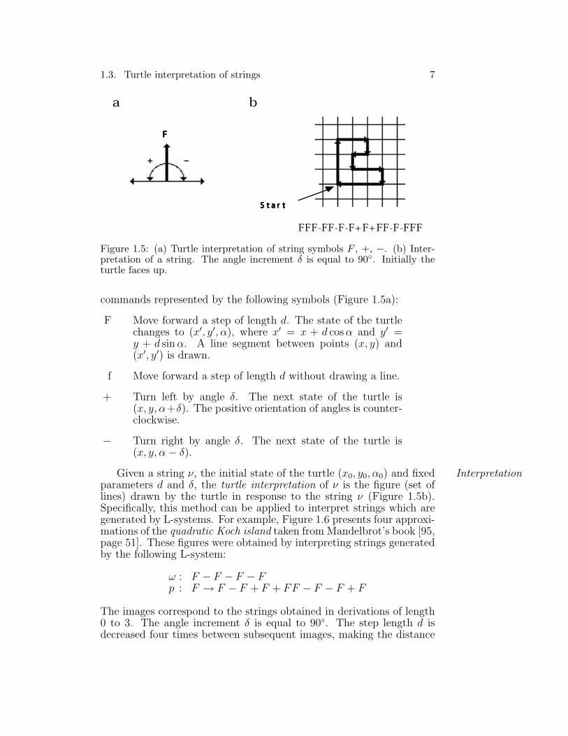
Figure 1.5: (a) Turtle interpretation of string symbols F , +, −. (b) Inter-pretation of a string. The angle increment δ is equal to 90◦. Initially theturtle faces up.

commands represented by the following symbols (Figure 1.5a):

F Move forward a step of length d. The state of the turtlechanges to (x′, y′, α), where x′ = x + d cos α and y′ =y + d sin α. A line segment between points (x, y) and(x′, y′) is drawn.

f Move forward a step of length d without drawing a line.

+ Turn left by angle δ. The next state of the turtle is(x, y, α+δ). The positive orientation of angles is counter-clockwise.

− Turn right by angle δ. The next state of the turtle is(x, y, α − δ).

Given a string ν, the initial state of the turtle (x0, y0, α0) and fixed Interpretationparameters d and δ, the turtle interpretation of ν is the figure (set oflines) drawn by the turtle in response to the string ν (Figure 1.5b).Specifically, this method can be applied to interpret strings which aregenerated by L-systems. For example, Figure 1.6 presents four approxi-mations of the quadratic Koch island taken from Mandelbrot’s book [95,page 51]. These figures were obtained by interpreting strings generatedby the following L-system:

ω : F − F − F − Fp : F → F − F + F + FF − F − F + F

The images correspond to the strings obtained in derivations of length0 to 3. The angle increment δ is equal to 90◦. The step length d isdecreased four times between subsequent images, making the distance


Figure 1.6: Generating a quadratic Koch island

between the endpoints of the successor polygon equal to the length ofthe predecessor segment.

The above example reveals a close relationship between Koch con- Kochconstructionsvs. L-systems

structions and L-systems. The initiator corresponds to the axiom andthe generator corresponds to the production successor. The predeces-sor F represents a single edge. L-systems specified in this way can beperceived as codings for Koch constructions. Figure 1.7 presents furtherexamples of Koch curves generated using L-systems. A slight compli-cation occurs if the curve is not connected; a second production (withthe predecessor f) is then required to keep components the proper dis-tance from each other (Figure 1.8). The ease of modifying L-systemsmakes them suitable for developing new Koch curves. For example, onecan start from a particular L-system and observe the results of insert-ing, deleting or replacing some symbols. A variety of curves obtainedthis way are shown in Figure 1.9.

1.3. Turtle interpretation of strings 9

Figure 1.7: Examples of Koch curves generated using L-systems: (a)Quadratic Koch island [95, page 52], (b) A quadratic modification of thesnowflake curve [95, page 139]

Figure 1.8: Combination of islands and lakes [95, page 121]


Figure 1.9: A sequence of Koch curves obtained by successive modificationof the production successor

1.4. Synthesis of DOL-systems 11

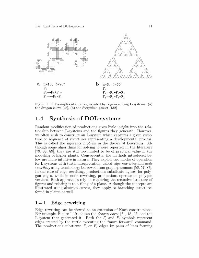
a n=10, δ=90◦FlFl→Fl+Fr+Fr→-Fl-Fr

b n=6, δ=60◦FrFl→Fr+Fl+FrFr→Fl-Fr-Fl

Figure 1.10: Examples of curves generated by edge-rewriting L-systems: (a)the dragon curve [48], (b) the Sierpinski gasket [132]

1.4 Synthesis of DOL-systems

Random modification of productions gives little insight into the rela-tionship between L-systems and the figures they generate. However,we often wish to construct an L-system which captures a given struc-ture or sequence of structures representing a developmental process.This is called the inference problem in the theory of L-systems. Al-though some algorithms for solving it were reported in the literature[79, 88, 89], they are still too limited to be of practical value in themodeling of higher plants. Consequently, the methods introduced be-low are more intuitive in nature. They exploit two modes of operationfor L-systems with turtle interpretation, called edge rewriting and noderewriting using terminology borrowed from graph grammars [56, 57, 87].In the case of edge rewriting, productions substitute figures for poly-gon edges, while in node rewriting, productions operate on polygonvertices. Both approaches rely on capturing the recursive structure offigures and relating it to a tiling of a plane. Although the concepts areillustrated using abstract curves, they apply to branching structuresfound in plants as well.

1.4.1 Edge rewriting

Edge rewriting can be viewed as an extension of Koch constructions.For example, Figure 1.10a shows the dragon curve [21, 48, 95] and theL-system that generated it. Both the Fl and Fr symbols representedges created by the turtle executing the “move forward” command.The productions substitute Fl or Fr edges by pairs of lines forming


an=4, δ=60◦FlFl→Fl+Fr++Fr-Fl--FlFl-Fr+Fr→-Fl+FrFr++Fr+Fl--Fl-Fr

bn=2, δ=90◦-FrFl→FlFl-Fr-Fr+Fl+Fl-Fr-FrFl+

Fr+FlFlFr-Fl+Fr+FlFl+Fr-FlFr-Fr-Fl+Fl+FrFr-

Fr→+FlFl-Fr-Fr+Fl+FlFr+Fl-FrFr-Fl-Fr+FlFrFr-Fl-FrFl+Fl+Fr-Fr-Fl+Fl+FrFr

Figure 1.11: Examples of FASS curves generated by edge-rewriting L-systems: (a) hexagonal Gosper curve [51], (b) quadratic Gosper curve [32]or E-curve [96]

left or right turns. Many interesting curves can be obtained assumingtwo types of edges, “left” and “right.” Figures 1.10b and 1.11 presentadditional examples.

The curves included in Figure 1.11 belong to the class of FASSFASS curveconstruction curves (an acronym for space-filling, self-avoiding, simple and self-

similar) [116], which can be thought of as finite, self-avoiding approxi-mations of curves that pass through all points of a square (space-fillingcurves [106]). McKenna [96] presented an algorithm for constructingFASS curves using edge replacement. It exploits the relationship be-tween such a curve and a recursive subdivision of a square into tiles.For example, Figure 1.12 shows the tiling that corresponds to the E-curve of Figure 1.11b. The polygon replacing an edge Fl (Figure 1.12a)approximately fills the square on the left side of Fl (b). Similarly, thepolygon replacing an edge Fr (c) approximately fills the square on theright side of that edge (d). Consequently, in the next derivation step,each of the 25 tiles associated with the curves (b) or (d) will be coveredby their reduced copies (Figure 1.11b). A recursive application of thisargument indicates that the whole curve is approximately space-filling.It is also self-avoiding due to the following two properties:


Fl→FlFl+Fr+Fr-Fl-Fl+Fr+FrFl-Fr-FlFlFr+Fl-Fr-FlFl-Fr+FlFr+Fr+Fl-Fl-FrFr+

Fr→-FlFl+Fr+Fr-Fl-FlFr-Fl+FrFr+Fl+Fr-FlFrFr+Fl+FrFl-Fl-Fr+Fr+Fl-Fl-FrFr

Figure 1.12: Construction of the E-curve on the square grid. Left and rightedges are distinguished by the direction of ticks.

• the generating polygon is self-avoiding, and

• no matter what the relative orientation of the polygons lying ontwo adjacent tiles, their union is a self-avoiding curve.

The first property is obvious, while the second can be verified by con-sidering all possible relative positions of a pair of adjacent tiles.

Using a computer program to search the space of generating poly-gons, McKenna found that the E-curve is the simplest FASS curveobtained by edge replacement in a square grid. Other curves requiregenerators with more edges (Figure 1.13). The relationship betweenedge rewriting and tiling of the plane extends to branching structures,providing a method for constructing and analyzing L-systems whichoperate according to the edge-rewriting paradigm (see Section 1.10.3).

1.4.2 Node rewriting

The idea of node rewriting is to substitute new polygons for nodes of the Subfigurespredecessor curve. In order to make this possible, turtle interpretationis extended by symbols which represent arbitrary subfigures. As shownin Figure 1.14, each subfigure A from a set of subfigures A is representedby:

• two contact points, called the entry point PA and the exit pointQA, and

• two direction vectors, called the entry vector �pA and the exit vector�qA.

During turtle interpretation of a string ν, a symbol A ∈ A incorporatesthe corresponding subfigure into a picture. To this end, A is translated


Figure 1.13: Examples of FASS curves generated on the square grid usingedge replacement: (a) a SquaRecurve (grid size 7 × 7), (b) an E-tour (gridsize 9 × 9). Both curves are from [96].

Figure 1.14: Description of a subfigure A


Ln RnLn+1 Rn+1

Ln+2 Rn+2

Figure 1.15: Recursive construction of the Hilbert curve [63] in terms ofnode replacement

and rotated in order to align its entry point PA and direction �pA withthe current position and orientation of the turtle. Having placed A, theturtle is assigned the resulting exit position QA and direction �qA.

For example, assuming that the contact points and directions of Recursiveformulassubfigures Ln and Rn are as in Figure 1.15, the figures Ln+1 and Rn+1

are captured by the following formulas:

Ln+1 = +RnF − LnFLn − FRn+Rn+1 = −LnF + RnFRn + FLn−

Suppose that curves L0 and R0 are given. One way of evaluating thestring Ln (or Rn) for n > 0 is to generate successive strings recur-sively, in the order of decreasing value of index n. For example, thecomputation of L2 would proceed as follows:

L2 = +R1F − L1FL1 − FR1+= +(−L0F + R0FR0 + FL0−)F − (+R0F − L0FL0 − FR0+)

F (+R0F − L0FL0 − FR0+) − F (−L0F + R0FR0 + FL0−)+


Thus, the generation of string Ln can be considered as a string-rewritingmechanism, where the symbols on the left side of the recursive formulasare substituted by corresponding strings on the right side. The substi-tution proceeds in a parallel way with F, + and − replacing themselves.Since all indices in any given string have the same value, they can bedropped, provided that a global count of derivation steps is kept. Con-sequently, string Ln can be obtained in a derivation of length n usingthe following L-system:

ω : Lp1 : L → +RF − LFL − FR+p2 : R → −LF + RFR + FL−

In order to complete the curve definition, it is necessary to specifythe subfigures represented by symbols L and R. In the special case ofPure curvespure curves [116], these subfigures are reduced to single points. Thus,one can assume that symbols L and R are erased (replaced by the emptystring) at the end of the derivation. Alternatively, they can be left inthe string and ignored by the turtle during string interpretation. Thissecond approach is consistent with previous definitions of turtle inter-pretation [109, 112]. A general discussion of the relationship betweenrecurrent formulas and L-systems is presented in [61, 62].

Construction of the L-system generating the Hilbert curve can beFASS curveconstruction extended to other FASS curves [116]. Consider an array of m×m square

tiles, each including a smaller square, called a frame. The edges of theframe run at some distance from the tile’s edges. Each frame bounds anopen self-avoiding polygon. The endpoints of this polygon coincide withthe two contact vertices of the frame. Suppose that a single-stroke linerunning through all tiles can be constructed by connecting the contactvertices of neighboring frames using short horizontal or vertical linesegments. A FASS curve can be constructed by the recursive repetitionof this connecting pattern. To this end, the array of m × m connectedtiles is considered a macrotile which contains an open polygon inscribedinto a macroframe. An array of m × m macrotiles is formed, and thepolygons inscribed into the macroframes are connected together. Thisconstruction is carried out recursively, with m × m macrotiles at leveln yielding one macrotile at level n + 1.

Tile arrangements suitable for the generation of FASS curves canbe found algorithmically, by searching the space of all possible arrange-ments on a grid of a given size. Examples of curves synthesized thisway are given in Figures 1.16 and 1.17.

As in the case of edge rewriting, the relationship between noderewriting and tilings of the plane extends to branching structures. Itoffers a method for synthesizing L-systems that generate objects with agiven recursive structure, and links methods for plant generation basedon L-systems with those using iterated function systems [7] (see Chap-ter 8).


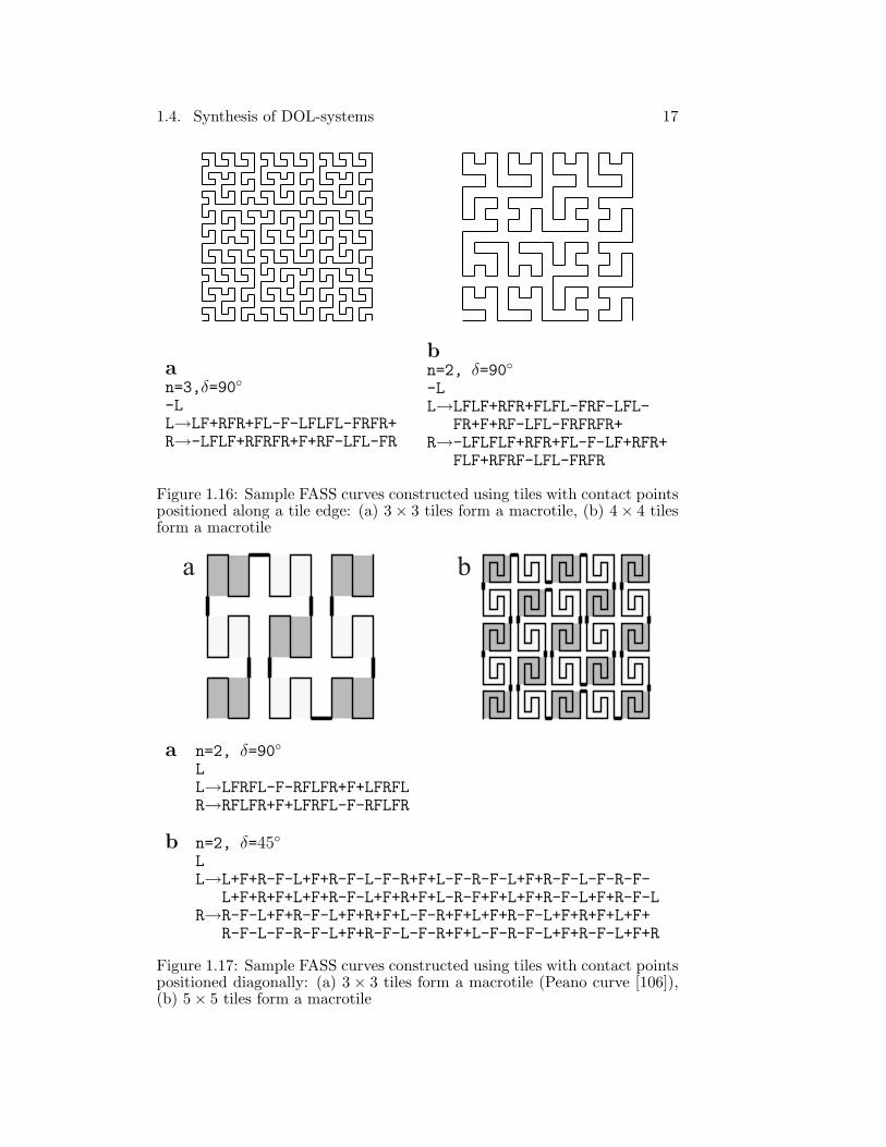
an=3,δ=90◦-LL→LF+RFR+FL-F-LFLFL-FRFR+R→-LFLF+RFRFR+F+RF-LFL-FR

bn=2, δ=90◦-LL→LFLF+RFR+FLFL-FRF-LFL-

FR+F+RF-LFL-FRFRFR+R→-LFLFLF+RFR+FL-F-LF+RFR+

FLF+RFRF-LFL-FRFR

Figure 1.16: Sample FASS curves constructed using tiles with contact pointspositioned along a tile edge: (a) 3 × 3 tiles form a macrotile, (b) 4 × 4 tilesform a macrotile

a n=2, δ=90◦LL→LFRFL-F-RFLFR+F+LFRFLR→RFLFR+F+LFRFL-F-RFLFR

b n=2, δ=45◦LL→L+F+R-F-L+F+R-F-L-F-R+F+L-F-R-F-L+F+R-F-L-F-R-F-

L+F+R+F+L+F+R-F-L+F+R+F+L-R-F+F+L+F+R-F-L+F+R-F-LR→R-F-L+F+R-F-L+F+R+F+L-F-R+F+L+F+R-F-L+F+R+F+L+F+

R-F-L-F-R-F-L+F+R-F-L-F-R+F+L-F-R-F-L+F+R-F-L+F+R

Figure 1.17: Sample FASS curves constructed using tiles with contact pointspositioned diagonally: (a) 3 × 3 tiles form a macrotile (Peano curve [106]),(b) 5 × 5 tiles form a macrotile


1.4.3 Relationship between edge andnode rewriting

The classes of curves that can be generated using the edge-rewriting andnode-rewriting techniques are not disjoint. For example, reconsider theL-system that generates the dragon curve using edge replacement:

ω : Fl

p1 : Fl → Fl + Fr+p2 : Fr → −Fl − Fr

Assume temporarily that a production predecessor can contain morethan one letter; thus an entire subword can be replaced by the successorof a single production (a formalization of this concept is termed pseudo-L-systems [109]). The dragon-generating L-system can be rewritten as:

ω : Flp1 : Fl → Fl + rF+p2 : rF → −Fl − rF

where the symbols l and r are not interpreted by the turtle. Productionp1 replaces the letter l by the string l + rF− while the leading letter Fis left intact. In a similar way, production p2 replaces the letter r bythe string −Fl−r and leaves the trailing F intact. Thus, the L-systemcan be transformed into node-rewriting form as follows:

ω : Flp1 : l → l + rF+p2 : r → −Fl − r

In practice, the choice between edge rewriting and node rewritingis often a matter of convenience. Neither approach offers an auto-matic, general method for constructing L-systems that capture givenstructures. However, the distinction between edge and node rewritingmakes it easier to understand the intricacies of L-system operation, andin this sense assists in the modeling task. Specifically, the problem offilling a region by a self-avoiding curve is biologically relevant, sincesome plant structures, such as leaves, may tend to fill a plane withoutoverlapping [38, 66, 67, 94].

1.5 Modeling in three dimensions

Turtle interpretation of L-systems can be extended to three dimensionsfollowing the ideas of Abelson and diSessa [1]. The key concept is torepresent the current orientation of the turtle in space by three vectors�H,�L, �U, indicating the turtle’s heading, the direction to the left, and thedirection up. These vectors have unit length, are perpendicular to each

1.5. Modeling in three dimensions 19

Figure 1.18: Controlling the turtle in three dimensions

other, and satisfy the equation �H × �L = �U. Rotations of the turtle arethen expressed by the equation

[�H ′ �L′ �U ′

]=

[�H �L �U

]R,

where R is a 3× 3 rotation matrix [40]. Specifically, rotations by angleα about vectors �U,�L and �H are represented by the matrices:

RU(α) =

cos α sin α 0− sin α cos α 0

0 0 1

RL(α) =

cos α 0 − sin α

0 1 0sin α 0 cos α

RH(α) =

1 0 0

0 cos α − sin α0 sin α cos α

The following symbols control turtle orientation in space (Figure 1.18):

+ Turn left by angle δ, using rotation matrix RU(δ).

− Turn right by angle δ, using rotation matrix RU(−δ).

& Pitch down by angle δ, using rotation matrix RL(δ).

∧ Pitch up by angle δ, using rotation matrix RL(−δ).

\ Roll left by angle δ, using rotation matrix RH(δ).

/ Roll right by angle δ, using rotation matrix RH(−δ).

| Turn around, using rotation matrix RU(180◦).

1.6. Branching structures 21

As an example of a three-dimensional object created using an L-system, consider the extension of the Hilbert curve shown in Figure 1.19.The L-system was constructed with the node-replacement techniquediscussed in the previous section, using cubes and “macrocubes” in-stead of tiles and macrotiles.

1.6 Branching structures

According to the rules presented so far, the turtle interprets a characterstring as a sequence of line segments. Depending on the segment lengthsand the angles between them, the resulting line is self-intersecting ornot, can be more or less convoluted, and may have some segmentsdrawn many times and others made invisible, but it always remainsjust a single line. However, the plant kingdom is dominated by branch-ing structures; thus a mathematical description of tree-like shapes andmethods for generating them are needed for modeling purposes. Anaxial tree [89, 117] complements the graph-theoretic notion of a rootedtree [108] with the botanically motivated notion of branch axis.

1.6.1 Axial trees

A rooted tree has edges that are labeled and directed. The edge se-quences form paths from a distinguished node, called the root or base,to the terminal nodes . In the biological context, these edges are re-ferred to as branch segments . A segment followed by at least one moresegment in some path is called an internode. A terminal segment (withno succeeding edges) is called an apex.

An axial tree is a special type of rooted tree (Figure 1.20). At eachof its nodes, at most one outgoing straight segment is distinguished.All remaining edges are called lateral or side segments. A sequence ofsegments is called an axis if:

• the first segment in the sequence originates at the root of the treeor as a lateral segment at some node,

• each subsequent segment is a straight segment, and

• the last segment is not followed by any straight segment in thetree.

Together with all its descendants, an axis constitutes a branch. Abranch is itself an axial (sub)tree.

Axes and branches are ordered. The axis originating at the root ofthe entire plant has order zero. An axis originating as a lateral segmentof an n-order parent axis has order n+1. The order of a branch is equalto the order of its lowest-order or main axis.


Figure 1.20: An axial tree

Figure 1.21: Sample tree generated using a method based on Horton–Strahler analysis of branching patterns


Figure 1.22: A tree production p and its application to the edge S in a treeT1

Axial trees are purely topological objects. The geometric connotationof such terms as straight segment, lateral segment and axis should beviewed at this point as an intuitive link between the graph-theoreticformalism and real plant structures.

The proposed scheme for ordering branches in axial trees was in-troduced originally by Gravelius [53]. MacDonald [94, pages 110–121]surveys this and other methods applicable to biological and geograph-ical data such as stream networks. Of special interest are methodsproposed by Horton [70, 71] and Strahler, which served as a basis forsynthesizing botanical trees [37, 152] (Figure 1.21).

1.6.2 Tree OL-systems

In order to model development of branching structures, a rewritingmechanism can be used that operates directly on axial trees. A rewrit-ing rule, or tree production, replaces a predecessor edge by a successoraxial tree in such a way that the starting node of the predecessor isidentified with the successor’s base and the ending node is identifiedwith the successor’s top (Figure 1.22).

A tree OL-system G is specified by three components: a set of edgelabels V , an initial tree ω with labels from V , and a set of tree produc-tions P . Given the L-system G, an axial tree T2 is directly derived froma tree T1, noted T1 ⇒ T2, if T2 is obtained from T1 by simultaneouslyreplacing each edge in T1 by its successor according to the productionset P . A tree T is generated by G in a derivation of length n if thereexists a sequence of trees T0, T1, . . . , Tn such that T0 = ω, Tn = T andT0 ⇒ T1 ⇒ . . . ⇒ Tn.


Figure 1.23: Bracketed string representation of an axial tree

1.6.3 Bracketed OL-systems

The definition of tree L-systems does not specify the data structure forrepresenting axial trees. One possibility is to use a list representationwith a tree topology. Alternatively, axial trees can be represented usingstrings with brackets [82]. A similar distinction can be observed in Kochconstructions, which can be implemented either by rewriting edges andpolygons or their string representations. An extension of turtle in-terpretation to strings with brackets and the operation of bracketedL-systems [109, 111] are described below.

Two new symbols are introduced to delimit a branch. They areinterpreted by the turtle as follows:

[ Push the current state of the turtle onto a pushdownStackoperations stack. The information saved on the stack contains the

turtle’s position and orientation, and possibly other at-tributes such as the color and width of lines being drawn.

] Pop a state from the stack and make it the current stateof the turtle. No line is drawn, although in general theposition of the turtle changes.

An example of an axial tree and its string representation are shownin Figure 1.23.

Derivations in bracketed OL-systems proceed as in OL-systems with-2D structuresout brackets. The brackets replace themselves. Examples of two-dimensional branching structures generated by bracketed OL-systemsare shown in Figure 1.24.

Figure 1.25 is an example of a three-dimensional bush-like structureBush-likestructure generated by a bracketed L-system. Production p1 creates three new

branches from an apex of the old branch. A branch consists of anedge F forming the initial internode, a leaf L and an apex A (whichwill subsequently create three new branches). Productions p2 and p3


an=5,δ=25.7◦FF→F[+F]F[-F]F

bn=5,δ=20◦FF→F[+F]F[-F][F]

cn=4,δ=22.5◦FF→FF-[-F+F+F]+

[+F-F-F]

dn=7,δ=20◦XX→F[+X]F[-X]+XF→FF

en=7,δ=25.7◦XX→F[+X][-X]FXF→FF

fn=5,δ=22.5◦XX→F-[[X]+X]+F[+FX]-XF→FF

Figure 1.24: Examples of plant-like structures generated by bracketed OL-systems. L-systems (a), (b) and (c) are edge-rewriting, while (d), (e) and(f) are node-rewriting.


n=7, δ=22.5◦

ω : Ap1 : A → [&FL!A]/////’[&FL!A]///////’[&FL!A]p2 : F → S ///// Fp3 : S → F Lp4 : L → [’’’∧∧{-f+f+f-|-f+f+f}]

Figure 1.25: A three-dimensional bush-like structure

specify internode growth. In subsequent derivation steps the internodegets longer and acquires new leaves. This violates a biological ruleof subapical growth (discussed in detail in Chapter 3), but producesan acceptable visual effect in a still picture. Production p4 specifiesthe leaf as a filled polygon with six edges. Its boundary is formedfrom the edges f enclosed between the braces { and } (see Chapter 5for further discussion). The symbols ! and ′ are used to decrementthe diameter of segments and increment the current index to the colortable, respectively.

Another example of a three-dimensional plant is shown in Fig-Plantwith flowers ure 1.26. The L-system can be described and analyzed in a way similar

to the previous one.


n=5, δ=18◦

ω : plantp1 : plant → internode + [ plant + flower] − − //

[ − − leaf ] internode [ + + leaf ] −[ plant flower ] + + plant flower

p2 : internode → F seg [// & & leaf ] [// ∧ ∧ leaf ] F segp3 : seg → seg F segp4 : leaf → [’ { +f−ff−f+ | +f−ff−f } ]p5 : flower → [ & & & pedicel ‘ / wedge //// wedge ////

wedge //// wedge //// wedge ]p6 : pedicel → FFp7 : wedge → [‘ ∧ F ] [ { & & & & −f+f | −f+f } ]

Figure 1.26: A plant generated by an L-system


1.7 Stochastic L-systems

All plants generated by the same deterministic L-system are identical.An attempt to combine them in the same picture would produce astriking, artificial regularity. In order to prevent this effect, it is nec-essary to introduce specimen-to-specimen variations that will preservethe general aspects of a plant but will modify its details.

Variation can be achieved by randomizing the turtle interpretation,the L-system, or both. Randomization of the interpretation alone hasa limited effect. While the geometric aspects of a plant — such asthe stem lengths and branching angles — are modified, the underly-ing topology remains unchanged. In contrast, stochastic applicationof productions may affect both the topology and the geometry of theplant. The following definition is similar to that of Yokomori [162] andEichhorst and Savitch [35].

A stochastic OL-system is an ordered quadruplet Gπ = 〈V, ω, P, π〉.L-systemThe alphabet V , the axiom ω and the set of productions P are definedas in an OL-system (page 4). Function π : P → (0, 1], called theprobability distribution, maps the set of productions into the set ofproduction probabilities. It is assumed that for any letter a ∈ V , thesum of probabilities of all productions with the predecessor a is equalto 1.

We will call the derivation µ ⇒ ν a stochastic derivation in Gπ if forDerivationeach occurrence of the letter a in the word µ the probability of applyingproduction p with the predecessor a is equal to π(p). Thus, differentproductions with the same predecessor can be applied to various occur-rences of the same letter in one derivation step.

A simple example of a stochastic L-system is given below.Example

ω : F

p1 : F.33→ F [+F ]F [−F ]F

p2 : F.33→ F [+F ]F

p3 : F.34→ F [−F ]F

The production probabilities are listed above the derivation symbol→. Each production can be selected with approximately the sameprobability of 1/3. Examples of branching structures generated by thisL-system with derivations of length 5 are shown in Figure 1.27. Notethat these structures look like different specimens of the same (albeitfictitious) plant species.

A more complex example is shown in Figure 1.28. The field consistsFlower fieldof four rows and four columns of plants. All plants are generated by astochastic modification of the L-system used to generate Figure 1.26.

1.7. Stochastic L-systems 29

Figure 1.27: Stochastic branching structures

Figure 1.28: Flower field


The essence of this modification is to replace the original productionp3 by the following three productions:

p′3 : seg.33→ seg [ // & & leaf ] [// ∧∧ leaf ] F seg

p′′3 : seg.33→ seg F seg

p′′′3 : seg.34→ seg

Thus, in any step of the derivation, the stem segment seg may eithergrow and produce new leaves (production p′3), grow without producingnew leaves (production p′′3), or not grow at all (production p′′′3 ). All threeevents occur with approximately the same probability. The resultingfield appears to consist of various specimens of the same plant species.If the same L-system was used again (with different seed values for therandom number generator), a variation of this image would be obtained.

1.8 Context-sensitive L-systems

Productions in OL-systems are context-free; i.e. applicable regardlessContext instringL-systems

of the context in which the predecessor appears. However, productionapplication may also depend on the predecessor’s context. This effect isuseful in simulating interactions between plant parts, due for example tothe flow of nutrients or hormones. Various context-sensitive extensionsof L-systems have been proposed and studied thoroughly in the past[62, 90, 128]. 2L-systems use productions of the form al < a > ar → χ,where the letter a (called the strict predecessor) can produce word χ ifand only if a is preceded by letter al and followed by ar. Thus, lettersal and ar form the left and the right context of a in this production.Productions in 1L-systems have one-sided context only; consequently,they are either of the form al < a → χ or a > ar → χ. OL-systems,1L-systems and 2L-systems belong to a wider class of IL-systems, alsocalled (k,l)-systems. In a (k,l)-system, the left context is a word oflength k and the right context is a word of length l.

In order to keep specifications of L-systems short, the usual notionof IL-systems has been modified here by allowing productions withdifferent context lengths to coexist within a single system. Further-more, context-sensitive productions are assumed to have precedenceover context-free productions with the same strict predecessor. Conse-quently, if a context-free and a context-sensitive production both applyto a given letter, the context-sensitive one should be selected. If no pro-duction applies, this letter is replaced by itself as previously assumedfor OL-systems.

1.8. Context-sensitive L-systems 31

Figure 1.29: The predecessor of a context-sensitive tree production (a)matches edge S in a tree T (b)

The following sample 1L-system makes use of context to simulate signal Signalpropagationpropagation throughout a string of symbols:

ω : baaaaaaaap1 : b < a → bp2 : b → a

The first few words generated by this L-system are given below:

baaaaaaaaabaaaaaaaaabaaaaaaaaabaaaaaaaaabaaaa· · ·

The letter b moves from the left side to the right side of the string.A context-sensitive extension of tree L-systems requires neighbor Context in tree

L-systemsedges of the replaced edge to be tested for context matching. A prede-cessor of a context-sensitive production p consists of three components:a path l forming the left context, an edge S called the strict predecessor,and an axial tree r constituting the right context (Figure 1.29). Theasymmetry between the left context and the right context reflects thefact that there is only one path from the root of a tree to a given edge,while there can be many paths from this edge to various terminal nodes.Production p matches a given occurrence of the edge S in a tree T if lis a path in T terminating at the starting node of S, and r is a subtree


of T originating at the ending node of S. The production can then beapplied by replacing S with the axial tree specified as the productionsuccessor.

The introduction of context to bracketed L-systems is more difficultContext inbracketedL-systems

than in L-systems without brackets, because the bracketed string repre-sentation of axial trees does not preserve segment neighborhood. Conse-quently, the context matching procedure may need to skip over symbolsrepresenting branches or branch portions. For example, Figure 1.29 in-dicates that a production with the predecessor BC < S > G[H]M canbe applied to symbol S in the string

ABC[DE][SG[HI[JK]L]MNO],

which involves skipping over symbols [DE] in the search for left context,and I[JK]L in the search for right context.

Within the formalism of bracketed L-systems, the left context canbe used to simulate control signals that propagate acropetally, i.e., fromthe root or basal leaves towards the apices of the modeled plant, whilethe right context represents signals that propagate basipetally, i.e., fromthe apices towards the root. For example, the following 1L-systemsimulates propagation of an acropetal signal in a branching structurethat does not grow:

#ignore : +−

ω : Fb[+Fa]Fa[−Fa]Fa[+Fa]Fa

p1 : Fb < Fa → Fb

Symbol Fb represents a segment already reached by the signal, whileFa represents a segment that has not yet been reached. The #ignorestatement indicates that the geometric symbols + and − should beconsidered as non-existent while context matching. Images representingconsecutive stages of signal propagation (corresponding to consecutivewords generated by the L-system under consideration) are shown inFigure 1.30a.

The propagation of a basipetal signal can be simulated in a similarway (Figure 1.30b):

#ignore : +−

ω : Fa[+Fa]Fa[−Fa]Fa[+Fa]Fb

p1 : Fa > Fb → Fb


Figure 1.30: Signal propagation in a branching structure: (a) acropetal, (b)basipetal

The operation of context-sensitive L-systems is examined further using L-systems ofHogeweg,Hesper andSmith

examples obtained by Hogeweg and Hesper [64]. In 1974, they pub-lished the results of an exhaustive study of 3,584 patterns generatedby a class of bracketed 2L-systems defined over the alphabet {0,1}.Some of these patterns had plant-like shapes. Subsequently, Smithsignificantly improved the quality of the generated images using state-of-the-art computer imagery techniques [136, 137]. Sample structuresgenerated by L-systems similar to those proposed by Hogeweg and Hes-per are shown in Figure 1.31. The differences are related to the geo-metric interpretation of the resulting strings. According to the originalinterpretation, consecutive branches are issued alternately to the leftand right, whereas turtle interpretation requires explicit specificationof branching angles within the L-system.


Figure 1.31: Examples of branching structures generated using L-systemsbased on the results of Hogeweg and Hesper [64]


a n=30,δ=22.5◦#ignore: +-FF1F1F10 < 0 > 0 → 00 < 0 > 1 → 1[+F1F1]0 < 1 > 0 → 10 < 1 > 1 → 11 < 0 > 0 → 01 < 0 > 1 → 1F11 < 1 > 0 → 01 < 1 > 1 → 0* < + > * → -* < - > * → +

b n=30,δ=22.5◦#ignore: +-FF1F1F10 < 0 > 0 → 10 < 0 > 1 → 1[-F1F1]0 < 1 > 0 → 10 < 1 > 1 → 11 < 0 > 0 → 01 < 0 > 1 → 1F11 < 1 > 0 → 11 < 1 > 1 → 0* < + > * → -* < - > * → +

c n=26, δ=25.75◦#ignore: +-FF1F1F10 < 0 > 0 → 00 < 0 > 1 → 10 < 1 > 0 → 00 < 1 > 1 → 1[+F1F1]1 < 0 > 0 → 01 < 0 > 1 → 1F11 < 1 > 0 → 01 < 1 > 1 → 0* < - > * → +* < + > * → -

d n=24, δ=25.75◦#ignore: +-FF0F1F10 < 0 > 0 → 10 < 0 > 1 → 00 < 1 > 0 → 00 < 1 > 1 → 1F11 < 0 > 0 → 11 < 0 > 1 → 1[+F1F1]1 < 1 > 0 → 11 < 1 > 1 → 0* < + > * → -* < - > * → +

e n=26, δ=22.5◦#ignore: +-FF1F1F10 < 0 > 0 → 00 < 0 > 1 → 1[-F1F1]0 < 1 > 0 → 10 < 1 > 1 → 11 < 0 > 0 → 01 < 0 > 1 → 1F11 < 1 > 0 → 11 < 1 > 1 → 0* < + > * → -* < - > * → +

Figure 1.31 (continued): L-systems of Hogeweg and Hesper


1.9 Growth functions

During the synthesis of a plant model it is often convenient to dis-Exponentialgrowth tinguish productions that specify the branching pattern from those

that describe elongation of plant segments. This separation can beobserved in some of the L-systems considered so far. For example, inL-systems (d), (e) and (f) from Figure 1.24 the first productions cap-ture the branching patterns, while the remaining productions, equal inall cases to F → FF , describe elongation of segments represented bysequences of symbols F . The number of letters F in a string χn orig-inating from a single letter F is doubled in each derivation step, thusthe elongation is exponential, with length(χn) = 2n.

A function that describes the number of symbols in a word in termsBasicproperties of its derivation length is called a growth function. The theory of L-

systems contains an extensive body of results on growth functions [62,127]. The central observation is that the growth functions of DOL-systems are independent of the letter ordering in the productions andderived words. Consequently, the relation between the number of letteroccurrences in a pair of words µ and ν, such that µ ⇒ ν, can beconveniently expressed using matrix notation.

Let G = 〈V, ω, P 〉 be a DOL-system and assume that letters ofthe alphabet V have been ordered, V = {a1, a2, . . . , am}. Construct asquare matrix Qm×m, where entry qij is equal to the number of occur-rences of letter aj in the successor of the production with predecessorai. Let ak

i denote the number of occurrences of letter ai in the wordx generated by G in a derivation of length k. The definition of directderivation in a DOL-system implies that

[ak

1 ak2 · · · ak

m

]

q11 q12 · · · q1m

q21 q22 · · · q2m...

qm1 qm2 · · · qmm

=

[ak+1

1 ak+12 · · · ak+1

m

].

This matrix notation is useful in the analysis of growth functions. Forexample, consider the following L-system:

ω : ap1 : a → abp2 : b → a

(1.2)

The relationship between the number of occurrences of letters a and bin two consecutively derived words is

[ak bk

] [1 11 0

]=

[ak+1 bk+1

]

1.9. Growth functions 37

orak+1 = ak + bk = ak + ak−1

for k = 1, 2, 3, . . . . From the axiom it follows that a0 = 1 anda1 = b0 = 0. Thus, the number of letters a in the strings gener-ated by the L-system specified in equation (1.2) grows according to theFibonacci series: 1, 1, 2, 3, 5, 8, . . . . This growth function was imple-mented by productions p2 and p3 in the L-system generating the bushin Figure 1.25 (page 26) to describe the elongation of its internodes.

Polynomial growth functions of arbitrary degree can be obtained Polynomialgrowthusing L-systems of the following form:

ω : a0

p1 : a0 → a0a1

p2 : a1 → a1a2

p3 : a2 → a2a3

p4 : a3 → a3a4...

The matrix Q is given below:

Q =

1 1 0 0 · · ·0 1 1 0 · · ·0 0 1 1 · · ·0 0 0 1 · · ·

...

Thus, for any i, k ≥ 1, the number aki of occurrences of symbol ai in

the string generated in a derivation of length k satisfies the equality

aki + ak

i+1 = ak+1i+1 .

Taking into consideration the axiom, the distribution of letters ai asa function of the derivation length is captured by the following table(only non-zero terms are shown):

k ak0 ak

1 ak2 ak

3 ak4 ak

5 ak6 ak

7

0 11 1 12 1 2 13 1 3 3 14 1 4 6 4 15 1 5 10 10 5 16 1 6 15 20 15 6 17 1 7 21 35 35 21 7 1

...


This table represents the Pascal triangle, thus for any k ≥ i ≥ 1 itsterms satisfy the following equality:

aki =

(ki

)=

k(k − 1) · · · (k − i + 1)

1 · 2 · · · i

Consequently, the number of occurrences of letter ai as a function ofthe derivation length k is expressed by a polynomial of degree i. Byidentifying letter ai with the turtle symbol F , it is possible to model in-ternode elongation expressed by polynomials of arbitrary degree i ≥ 0.This observation was generalized by Szilard [140], who developed an al-gorithm for constructing a DOL-system with growth functions specifiedby any positive, nondecreasing polynomials with integer coefficients [62,page 276].

The examples of growth functions considered so far include expo-Characterizationnential and polynomial functions. Rozenberg and Salomaa [127, pages30–38] show that, in general, the growth function fG(n) of any DOL-system G = 〈V, ω, P 〉 is a combination of polynomial and exponentialfunctions:

fG(n) =s∑

i=1

Pi(n)ρni for n ≥ n0, (1.3)

where Pi(n) denotes a polynomial with integer coefficients, ρi is a non-negative integer, and n0 is the total number of letters in the alphabetV . Unfortunately, many growth processes observed in nature cannot bedescribed by equation (1.3). Two approaches are then possible withinthe framework of the theory of L-systems.

The first is to extend the size n0 of the alphabet V , so that theSigmoidalgrowth growth process of interest will be captured by the initial derivation

steps, ω = µ0 ⇒ µ1 ⇒ · · · ⇒ µn0 , before equation (1.3) starts to apply.For example, the L-system

ω : a0

pi : ai → ai+1b0 for i < kpk+j : bj → bj+1F for j < l

(1.4)

over the alphabet V = {a0, a1, ..., ak}∪{b0, b1, ..., bl}∪{F} can be usedto approximate a sigmoidal elongation of a segment represented by asequence of symbols F (Figure 1.32). The term sigmoidal refers to afunction with a plot in the shape of the letter S. Such functions arecommonly found in biological processes [143], with the initial part ofthe curve representing the growth of a young organism, and the latterpart corresponding to the organism close to its final size.

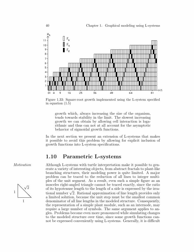
The second approach to the synthesis of growth functions out-side the class captured by equation (1.3) is to use context-sensitiveSquare-root

growth L-systems. For example, the following 2L-system has a growth func-tion given by fG(n) = �√n + 4, where �x is the floor function.

1.9. Growth functions 39

Figure 1.32: A sigmoidal growth function implemented using the L-systemin equation (1.4), for k = l = 20

ω : XFuFaXp1 : Fu < Fa > Fa → Fu

p2 : Fu < Fa > X → FdFa

p3 : Fa < Fa > Fd → Fd

p4 : X < Fa > Fd → Fu

p5 : Fu → Fa

p6 : Fd → Fa

(1.5)

The operation of this L-system is illustrated in Figure 1.33. Produc-tions p1 and p3, together with p5 and p6, propagate symbols Fu and Fd

up and down the string of symbols µ. Productions p2 and p4 change thepropagation direction, after symbol X marking a string end has beenreached by Fu or Fd, respectively. In addition, p2 extends the stringwith a symbol Fa. Thus, the number of derivation steps increases bytwo between consecutive applications of production p2. As a result,string extension occurs at derivation steps n expressed by the squareof the string length, which yields the growth function �√n + 4.

In practice it is often difficult, if not impossible, to find L-systems Limitationswith the required growth functions. Vitanyi [153] illustrates this byreferring to sigmoidal curves:

If we want to obtain sigmoidal growth curves with theoriginal L-systems then not even the introduction of cellinteraction can help us out. In the first place, we end upconstructing quite unlikely flows of messages through theorganism, which are more suitable to electronic computers,and in fact give the organism universal computing power.Secondly, and this is more fundamental, we can not obtain


Figure 1.33: Square-root growth implemented using the L-system specifiedin equation (1.5)

growth which, always increasing the size of the organism,tends towards stability in the limit. The slowest increasinggrowth we can obtain by allowing cell interaction is loga-rithmic and thus can not at all account for the asymptoticbehavior of sigmoidal growth functions.

In the next section we present an extension of L-systems that makesit possible to avoid this problem by allowing for explicit inclusion ofgrowth functions into L-system specifications.

1.10 Parametric L-systems

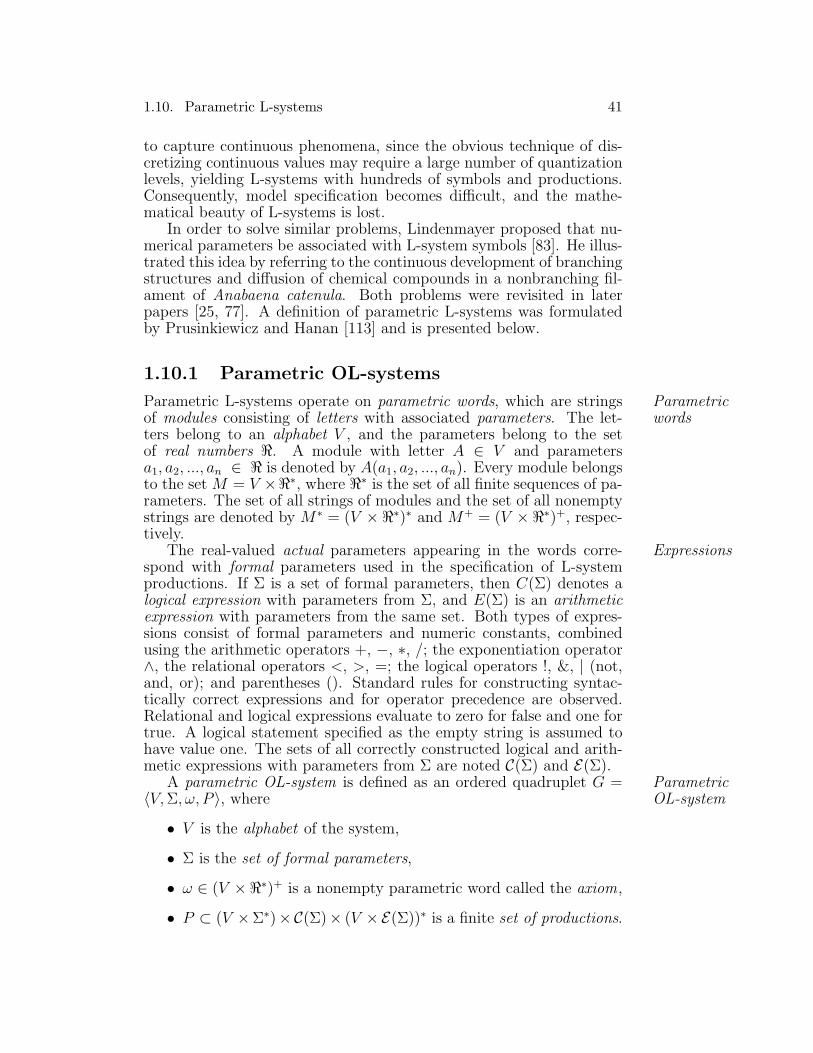
Although L-systems with turtle interpretation make it possible to gen-Motivationerate a variety of interesting objects, from abstract fractals to plant-likebranching structures, their modeling power is quite limited. A majorproblem can be traced to the reduction of all lines to integer multi-ples of the unit segment. As a result, even such a simple figure as anisosceles right-angled triangle cannot be traced exactly, since the ratioof its hypotenuse length to the length of a side is expressed by the irra-tional number

√2. Rational approximation of line length provides only

a limited solution, because the unit step must be the smallest common

��

��

1

1

√2

denominator of all line lengths in the modeled structure. Consequently,the representation of a simple plant module, such as an internode, mayrequire a large number of symbols. The same argument applies to an-gles. Problems become even more pronounced while simulating changesto the modeled structure over time, since some growth functions can-not be expressed conveniently using L-systems. Generally, it is difficult

1.10. Parametric L-systems 41

to capture continuous phenomena, since the obvious technique of dis-cretizing continuous values may require a large number of quantizationlevels, yielding L-systems with hundreds of symbols and productions.Consequently, model specification becomes difficult, and the mathe-matical beauty of L-systems is lost.

In order to solve similar problems, Lindenmayer proposed that nu-merical parameters be associated with L-system symbols [83]. He illus-trated this idea by referring to the continuous development of branchingstructures and diffusion of chemical compounds in a nonbranching fil-ament of Anabaena catenula. Both problems were revisited in laterpapers [25, 77]. A definition of parametric L-systems was formulatedby Prusinkiewicz and Hanan [113] and is presented below.

1.10.1 Parametric OL-systems

Parametric L-systems operate on parametric words, which are strings Parametricwordsof modules consisting of letters with associated parameters. The let-

ters belong to an alphabet V , and the parameters belong to the setof real numbers �. A module with letter A ∈ V and parametersa1, a2, ..., an ∈ � is denoted by A(a1, a2, ..., an). Every module belongsto the set M = V ×�∗, where �∗ is the set of all finite sequences of pa-rameters. The set of all strings of modules and the set of all nonemptystrings are denoted by M∗ = (V ×�∗)∗ and M+ = (V ×�∗)+, respec-tively.

The real-valued actual parameters appearing in the words corre- Expressionsspond with formal parameters used in the specification of L-systemproductions. If Σ is a set of formal parameters, then C(Σ) denotes alogical expression with parameters from Σ, and E(Σ) is an arithmeticexpression with parameters from the same set. Both types of expres-sions consist of formal parameters and numeric constants, combinedusing the arithmetic operators +, −, ∗, /; the exponentiation operator∧, the relational operators <, >, =; the logical operators !, &, | (not,and, or); and parentheses (). Standard rules for constructing syntac-tically correct expressions and for operator precedence are observed.Relational and logical expressions evaluate to zero for false and one fortrue. A logical statement specified as the empty string is assumed tohave value one. The sets of all correctly constructed logical and arith-metic expressions with parameters from Σ are noted C(Σ) and E(Σ).

A parametric OL-system is defined as an ordered quadruplet G = ParametricOL-system〈V, Σ, ω, P 〉, where

• V is the alphabet of the system,

• Σ is the set of formal parameters,

• ω ∈ (V ×�∗)+ is a nonempty parametric word called the axiom,

• P ⊂ (V ×Σ∗)×C(Σ)× (V ×E(Σ))∗ is a finite set of productions.


The symbols : and → are used to separate the three components of aproduction: the predecessor, the condition and the successor. For exam-ple, a production with predecessor A(t), condition t > 5 and successorB(t + 1)CD(t ∧ 0.5, t − 2) is written as

A(t) : t > 5 → B(t + 1)CD(t ∧ 0.5, t − 2). (1.6)

A production matches a module in a parametric word if the followingDerivationconditions are met:

• the letter in the module and the letter in the production prede-cessor are the same,

• the number of actual parameters in the module is equal to thenumber of formal parameters in the production predecessor, and

• the condition evaluates to true if the actual parameter values aresubstituted for the formal parameters in the production.

A matching production can be applied to the module, creating a stringof modules specified by the production successor. The actual parame-ter values are substituted for the formal parameters according to theirposition. For example, production (1.6) above matches a module A(9),since the letter A in the module is the same as in the production pre-decessor, there is one actual parameter in the module A(9) and oneformal parameter in the predecessor A(t), and the logical expressiont > 5 is true for t = 9. The result of the application of this productionis a parametric word B(10)CD(3, 7).

If a module a produces a parametric word χ as the result of aproduction application in an L-system G, we write a �→ χ. Given aparametric word µ = a1a2...am, we say that the word ν = χ1χ2...χm

is directly derived from (or generated by) µ and write µ =⇒ ν if andonly if ai �→ χi for all i = 1, 2, ...,m. A parametric word ν is generatedby G in a derivation of length n if there exists a sequence of wordsµ0, µ1, ..., µn such that µ0 = ω, µn = ν and µ0 =⇒ µ1 =⇒ ... =⇒ µn.

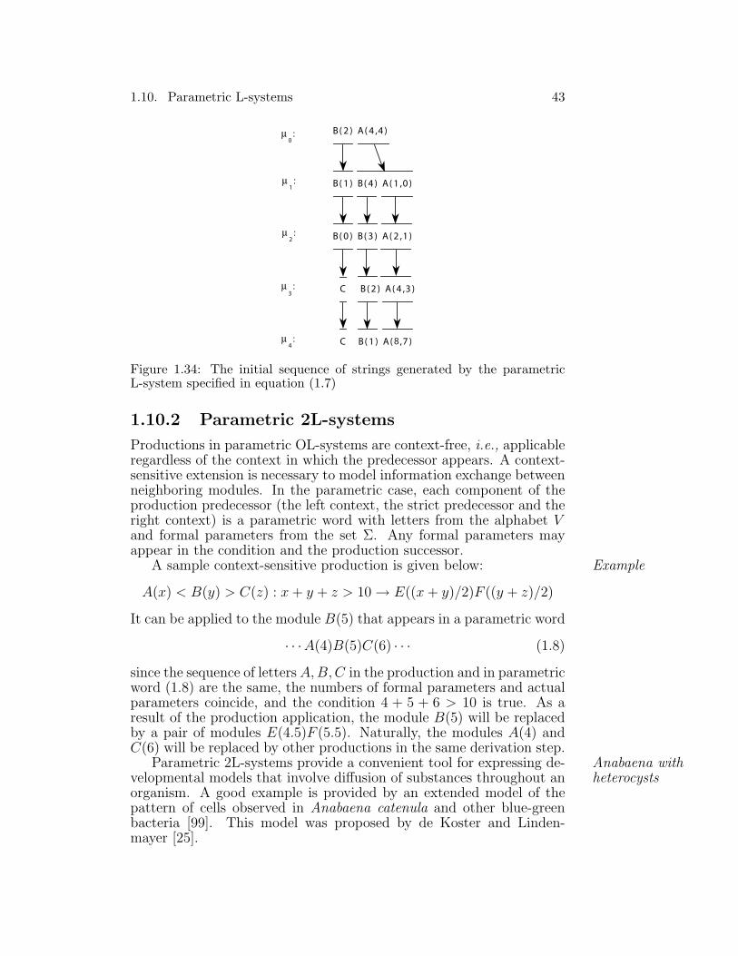
An example of a parametric L-system is given below.Example

ω : B(2)A(4, 4)p1 : A(x, y) : y <= 3 → A(x ∗ 2, x + y)p2 : A(x, y) : y > 3 → B(x)A(x/y, 0)p3 : B(x) : x < 1 → Cp4 : B(x) : x >= 1 → B(x − 1)

(1.7)

As in the case of non-parametric L-systems, it is assumed that a modulereplaces itself if no matching production is found in the set P . Thewords obtained in the first few derivation steps are shown in Figure 1.34.


Figure 1.34: The initial sequence of strings generated by the parametricL-system specified in equation (1.7)

1.10.2 Parametric 2L-systems

Productions in parametric OL-systems are context-free, i.e., applicableregardless of the context in which the predecessor appears. A context-sensitive extension is necessary to model information exchange betweenneighboring modules. In the parametric case, each component of theproduction predecessor (the left context, the strict predecessor and theright context) is a parametric word with letters from the alphabet Vand formal parameters from the set Σ. Any formal parameters mayappear in the condition and the production successor.

A sample context-sensitive production is given below: Example

A(x) < B(y) > C(z) : x + y + z > 10 → E((x + y)/2)F ((y + z)/2)

It can be applied to the module B(5) that appears in a parametric word

· · ·A(4)B(5)C(6) · · · (1.8)

since the sequence of letters A,B,C in the production and in parametricword (1.8) are the same, the numbers of formal parameters and actualparameters coincide, and the condition 4 + 5 + 6 > 10 is true. As aresult of the production application, the module B(5) will be replacedby a pair of modules E(4.5)F (5.5). Naturally, the modules A(4) andC(6) will be replaced by other productions in the same derivation step.

Parametric 2L-systems provide a convenient tool for expressing de- Anabaena withheterocystsvelopmental models that involve diffusion of substances throughout an

organism. A good example is provided by an extended model of thepattern of cells observed in Anabaena catenula and other blue-greenbacteria [99]. This model was proposed by de Koster and Linden-mayer [25].


#define CH 900 /* high concentration */#define CT 0.4 /* concentration threshold */#define ST 3.9 /* segment size threshold */#include H /* heterocyst shape specification */#ignore f ∼ H

ω : -(90)F(0,0,CH)F(4,1,CH)F(0,0,CH)

p1 : F(s,t,c) : t=1 & s>=6 →F(s/3*2,2,c)f(1)F(s/3,1,c)

p2 : F(s,t,c) : t=2 & s>=6 →F(s/3,2,c)f(1)F(s/3*2,1,c)

p3 : F(h,i,k) < F(s,t,c) > F(o,p,r) : s>ST|c>CT →F(s+.1,t,c+0.25*(k+r-3*c))

p4 : F(h,i,k) < F(s,t,c) > F(o,p,r) : !(s>ST|c>CT) →F(0,0,CH) ∼ H(1)

p5 : H(s) : s<3 → H(s*1.1)

L-system 1.1: Anabaena catenula

Generally, the bacteria under consideration form a nonbranching fila-ment consisting of two classes of cells: vegetative cells and heterocysts.Usually, the vegetative cells divide and produce two daughter vegeta-tive cells. This mechanism is captured by the L-system specified inequation (1.1) and Figure 1.4 (page 5). However, in some cases thevegetative cells differentiate into heterocysts. Their distribution formsa well-defined pattern, characterized by a relatively constant numberof vegetative cells separating consecutive heterocysts. How does theorganism maintain constant spacing of heterocysts while growing? Themodel explains this phenomenon using a biologically well-motivatedhypothesis that heterocyst distribution is regulated by nitrogen com-pounds produced by the heterocysts, transported from cell to cell acrossthe filament, and decayed in the vegetative cells. If the compound’sconcentration in a young vegetative cell falls below a specific level, thiscell differentiates into a heterocyst (L-system 1.1).

The #define statements assign values to numerical constants usedin the L-system. The #include statement specifies the shape of a het-erocyst (a disk) by referring to a library of predefined shapes (see Sec-tion 5.1). Cells are represented by modules F (s, t, c), where s standsfor cell length, t is cell type (0 - heterocyst, 1 and 2 - vegetative types1),

1The model of Anabaena introduced in Section 1.2 distinguished between fourtypes of cells: ar, br, al and bl. Cells b do not divide and can be considered as youngforms of the corresponding cells a. Thus, the vegetative type 1 considered hereembraces cells ar and br, while type 2 embraces al and bl. The formal relationshipbetween the four-cell and two-cell models is further discussed in Chapter 6.


Figure 1.35: Development of Anabaena catenula with heterocysts, simulatedusing parametric L-system 1.1

and c represents the concentration of nitrogen compounds. Productionsp1 and p2 describe division of the vegetative cells. They each create twodaughter cells of unequal length. The difference between cells of type1 and 2 lies in the ordering of the long and short daughter cells. Pro-duction p3 captures the processes of transportation and decay of thenitrogen compounds. Their concentration c is related to the concen-tration in the neighboring cells k and r, and changes in each derivationstep according to the formula

c′ = c + 0.25(k + r − 3 ∗ c).

Production p4 describes differentiation of a vegetative cell into a hete-rocyst. The condition specifies that this process occurs when the celllength does not exceed the threshold value ST = 3.9 (which meansthat the cell is young enough), and the concentration of the nitrogencompounds falls below the threshold value CT = 0.4. Production p5

describes the subsequent growth of the heterocyst.Snapshots of the developmental sequence of Anabaena are given

in Figure 1.35. The vegetative cells are shown as rectangles, coloredaccording to the concentration of the nitrogen compounds (white meanslow concentration). The heterocysts are represented as red disks. Thevalues of parameters CH, CT and ST were selected to provide the


correct distribution of the heterocysts, and correspond closely to thevalues reported in [25]. The mathematical model made it possible toestimate these parameters, although they are not directly observable.

1.10.3 Turtle interpretation of parametric words

If one or more parameters are associated with a symbol interpreted bythe turtle, the value of the first parameter controls the turtle’s state.If the symbol is not followed by any parameter, default values specifiedoutside the L-system are used as in the non-parametric case. The basicset of symbols affected by the introduction of parameters is listed below.

F (a) Move forward a step of length a > 0. The position of theturtle changes to (x′, y′, z′), where x′ = x + a�Hx, y′ = y + a�Hy

and z′ = z + a�Hz. A line segment is drawn between points(x, y, z) and (x′, y′, z′).

f(a) Move forward a step of length a without drawing a line.

+(a) Rotate around �U by an angle of a degrees. If a is positive, theturtle is turned to the left and if a is negative, the turn is tothe right.

&(a) Rotate around �L by an angle of a degrees. If a is positive,the turtle is pitched down and if a is negative, the turtle ispitched up.

/(a) Rotate around �H by an angle of a degrees. If a is positive, theturtle is rolled to the right and if a is negative, it is rolled tothe left.

It should be noted that symbols +, &, ∧, and / are used both asletters of the alphabet V and as operators in logical and arithmeticexpressions. Their meaning depends on the context.

The following examples illustrate the operation of parametric L-Row of treessystems with turtle interpretation. The first L-system is a coding ofa Koch construction generating a variant of the snowflake curve (Fig-ure 1.1 on page 2). The initiator (production predecessor) is the hy-potenuse AB of a right triangle ABC (Figure 1.36). The first and thefourth edge of the generator subdivide AB into segments AD and DB,while the remaining two edges traverse the altitude CD in opposite di-rections. From elementary geometry it follows that the lengths of thesesegments satisfy the equations

q = c − p and h =√

pq.

The edges of the generator can be associated with four triangles thatare similar to ABC and tile it without gaps. According to the relation-ship between curve construction by edge rewriting and planar tilings


Figure 1.36: Construction of the generator for a “row of trees.” The edgesare associated with triangles indicated by ticks.

(Section 1.4.1), the generated curve will approximately fill the triangleABC. The corresponding L-system is given below:

#define c 1#define p 0.3#define q c − p#define h (p ∗ q) ∧ 0.5

ω : F (1)p1 : F (x) → F (x ∗ p) + F (x ∗ h) −−F (x ∗ h) + F (x ∗ q)

The resulting curve is shown in Figure 1.37a. In order to bettervisualize its structure, the angle increment has been set to 86◦ insteadof 90◦. The curve fills different areas with unequal density. This resultsfrom the fact that all edges, whether long or short, are replaced bythe generator in every derivation step. A modified curve that fills theunderlying triangle in a more uniform way is shown in Figure 1.37b. Itwas obtained by delaying the rewriting of shorter segments with respectto the longer ones, as specified by the following L-system.

ω : F (1, 0)p1 : F (x, t) : t = 0 → F (x ∗ p, 2) + F (x ∗ h, 1)−

−F (x ∗ h, 1) + F (x ∗ q, 0)p2 : F (x, t) : t > 0 → F (x, t − 1)

The next example makes use of node rewriting (Section 1.4.2). The Branchingstructureconstruction recursively subdivides a rectangular tile ABCD into two

tiles, AEFD and BCFE, similar to ABCD (Figure 1.38). The lengthsof the edges form the proportion

a

b=

b12a,


Figure 1.37: Two curves suggesting a “row of trees.” Curve (b) is from [95,page 57].

which implies that b = a/√

2. Each tile is associated with a single-pointframe lying in the tile center. The tiles are connected by a branchingline specified by the following L-system:

#define R 1.456ω : A(1)p1 : A(s) → F (s)[+A(s/R)][−A(s/R)]

(1.9)

The ratio of branch sizes R slightly exceeds the theoretical value of√2. As a result, the branching structure shown in Figure 1.39 is self-

avoiding. The angle increment was set arbitrarily to δ = 85◦.The L-system in equation (1.9) operates by appending segments

of decreasing length to the structures obtained in previous derivationsteps. Once a segment has been incorporated, its length does notchange. A structure with identical proportions can be obtained by


Figure 1.38: Tiling associated with a space-filling branching pattern

Figure 1.39: A branching pattern generated by the L-system specified inequation (1.9)


Figure 1.40: Initial sequences of figures generated by the L-systems specifiedin equations (1.9) and (1.10)

appending segments of constant length and increasing the lengths ofpreviously created segments by constant R in each derivation step. Thecorresponding L-system is given below.

ω : Ap1 : A → F (1)[+A][−A]p2 : F (s) → F (s ∗ R)

(1.10)

The initial sequence of structures obtained by both L-systems arecompared in Figure 1.40. Sequence (a) emphasizes the fractal characterof the resulting structure. Sequence (b) suggests the growth of a tree.The next two chapters show that this is not a mere coincidence, andthe L-system specified in equation (1.10) is a simple, but in principlecorrect, developmental model of a sympodial branching pattern foundin many herbaceous plants and trees.

chapter 1 graphical modeling using l-systems

Documents