chapter 1 introduction - computing science - simon …stella/papers/simontangmsc.doc · web viewdr....

Towards Real-Time Magnetic Resonance Teleradiology

Over The Internet

by

Simon Tang

B.Sc., Simon Fraser University, 1994

THESIS SUBMITTED IN PARTIAL FULFILLMENT OF

THE REQUIREMENTS FOR THE DEGREE OF

MASTER OF SCIENCE

In the School

of

Computing Science

Simon Tang 1999

SIMON FRASER UNIVERSITY

April 1999

All rights reserved. This work may not be

reproduced in whole or in part, by photocopy

or other means, without the permission of the author.

ApprovalName: Simon Tang

Degree: Master of Science

Title of thesis: Towards Real-Time Magnetic Resonance Teleradiology Over The Internet

Examining Committee:

Dr. William Havens

Chair

Dr. Stella AtkinsSenior Supervisor

Dr. Tom CalvertSupervisor

Dr. Dave FracchiaSupervisor

Dr. Tiko KamedaSFU Examiner

Date Approved

ii

Abstract

Teleradiology involves transmitting high-resolution medical images from one remote site

to another and displaying the images effectively so that radiologists can perform the

proper diagnosis. Recent advances in medicine combined with those in technology have

resulted in a vast array of medical imaging techniques, but due to the characteristics of

these images, there are challenges to overcome in order to transmit these images

efficiently. We describe in this thesis a prototype system that implements three image

retrieval algorithms (Full-resolution, Scaled, and Pre-compressed) for retrieving

magnetic resonance (MR) images that are stored on a web server. The MR images are

displayed on a computer monitor instead of a traditional light screen.

Our prototype system consists of a Java-based Image Viewer, and a web server

extension component called, Image Servlet. The latter is responsible for transmitting the

MR images to the Image Viewer. This thesis also investigates the feasibility of achieving

real-time performance in retrieving and viewing MR images over the Internet using

HTTP/1.0 protocol. We have conducted experiments to measure the round trip time of

retrieving the MR images. Based on the findings from the experiments, the three image

retrieval algorithms are compared and a discussion of their appropriateness for

teleradiology is presented.

iii

Dedication

To my wife Rita for her continuous encouragement and support.

iv

Acknowledgments

I would like to thank Dr. Stella Atkins for her guidance and support throughout this thesis

work. She has given me a tremendous amount of feedback for improving on the work. I

also would like to thank my supervisors Dr. Tom Calvert and Dr. Dave Fracchia for

providing me with their time and expertise.

I am grateful to have Johanna van der Heyden for the many discussions and ideas.

Last, but not least, there are my grand parents, and parents for always being patient with

me and for continuing to give me their support.

v

Table of Contents

APPROVAL.................................................................................................................................... II

ABSTRACT................................................................................................................................... III

DEDICATION................................................................................................................................ IV

ACKNOWLEDGMENTS................................................................................................................V

TABLE OF CONTENTS................................................................................................................VI

LIST OF FIGURES......................................................................................................................VIII

LIST OF TABLES......................................................................................................................... IX

CHAPTER 1 INTRODUCTION.......................................................................................................1

1.1 MOTIVATION AND OBJECTIVES.................................................................................................1

1.2 METHOD................................................................................................................................. 1

1.3 ORGANIZATION....................................................................................................................... 2

CHAPTER 2 BACKGROUND........................................................................................................3

2.1 THE INTERNET........................................................................................................................ 3

2.1.1 Introduction.................................................................................................................... 3

2.1.2 The Basics..................................................................................................................... 4

2.1.3 Performance.................................................................................................................. 5

2.2 TELEMEDICINE........................................................................................................................ 7

2.2.1 Introduction.................................................................................................................... 7

2.2.2 Imaging Aspects............................................................................................................8

2.2.3 Imaging Standards and DICOM...................................................................................11

CHAPTER 3 MAGNETIC RESONANCE IMAGE VIEWER..........................................................12

3.1 INTRODUCTION......................................................................................................................12

3.2 RETRIEVING MR IMAGES THROUGH HTTP.............................................................................14

3.2.1 Image Viewer Enhancements......................................................................................14

3.2.2 Image Servlet...............................................................................................................15

3.2.3 Image Retrieval Algorithms..........................................................................................17

3.2.3 Process Flow...............................................................................................................22

CHAPTER 4 PERFORMANCE EVALUATION............................................................................24

vi

4.1 INTRODUCTION......................................................................................................................24

4.2 EXPERIMENT DESIGN............................................................................................................26

4.2.1 Objective...................................................................................................................... 26

4.2.2 Experiment Setup........................................................................................................26

4.2.3 Time Components........................................................................................................27

4.2.4 Timers..........................................................................................................................29

CHAPTER 5 RESULTS AND DISCUSSIONS.............................................................................30

5.1 END TO END OBSERVATIONS.................................................................................................30

5.2 DETAILED OBSERVATIONS.....................................................................................................31

5.2.1 Observations for Full-resolution Image Retrieval Algorithm.........................................31

5.2.2 Observations for Scaled Image Retrieval Algorithm.....................................................32

5.2.3 Observations for Pre-compressed Image Retrieval Algorithm.....................................33

5.3 DID WE ACHIEVE REAL-TIME MR IMAGE VIEWING?................................................................34

5.3.1 Factors Contributing to the RTT...................................................................................35

5.3.2 Which Algorithm is Better?...........................................................................................38

CHAPTER 6 CONCLUSION AND SUMMARY............................................................................40

6.1 CONCLUSION........................................................................................................................40

6.2 FUTURE RESEARCH..............................................................................................................41

REFERENCES............................................................................................................................. 43

APPENDIX A : FILM DESCRIPTOR FILE FORMAT...................................................................45

APPENDIX B : EXPERIMENT DATA...........................................................................................46

B.1 Full-resolution algorithm data.........................................................................................46

B.2 Scaled algorithm data.....................................................................................................47

B.3 Pre-compressed algorithm data......................................................................................48

vii

List of FiguresFigure 1: Four medical image modalities (clockwise from top left): CT Image, MR Image,

Ultrasound image, and PET scan image.................................................................................9

Figure 2: A light-screen that radiologists use to look at MR films..................................................12

Figure 3: The Image Viewer in action: a) Before enlarging the selected focal nodes, b) After

enlarging the selected foci....................................................................................................13

Figure 4: Image Servlet architectural diagram..............................................................................17

Figure 5: Comparing different compression ratio..........................................................................20

Figure 6: Comparing a) The original image (Top) with b) Scale-down image (Bottom left) and c)

Compressed image (Bottom right)........................................................................................20

Figure 7: Process Flow Diagram...................................................................................................22

Figure 8: Timimg components for each of the algorithms.............................................................29

Figure 9: Total image retrieval times.............................................................................................30

Figure 10: Full-resolution Algorithm Time Components................................................................31

Figure 11: Scaled Algorithm Time Components...........................................................................32

Figure 12: Pre-compressed Algorithm Time Components............................................................33

Figure 13: Components that were used in the prototype system..................................................35

viii

List of TablesTable 1: Selected HTTP Header Fields..........................................................................................4

Table 2: ImageServlet parameters................................................................................................16

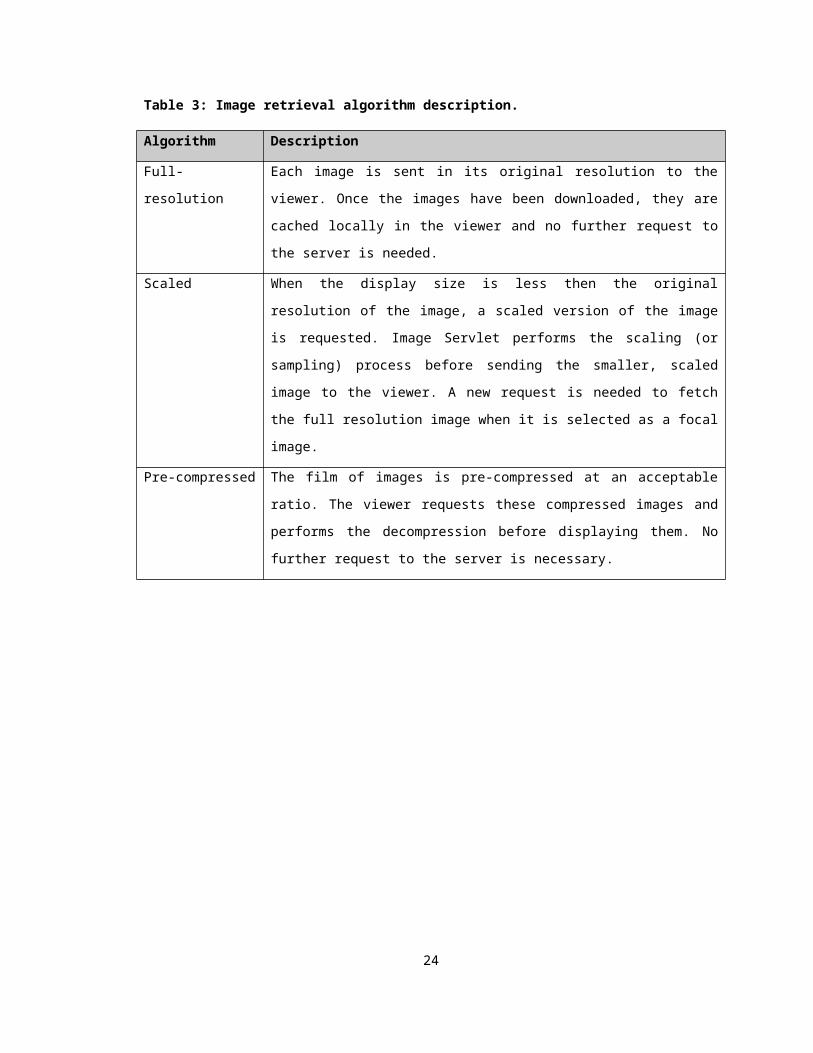
Table 3: Image retrieval algorithm description..............................................................................18

Table 4: Process Flow Descriptions..............................................................................................23

Table 5: Experimental Setups.......................................................................................................27

Table 6: Theoretical Transmission Time for the Three Image Retrieval Algorithms......................27

Table 7: Average image retrieval times (in milliseconds) from 10 trials with 16 images................30

Table 8: Comparisons between Java interpreter and JIT compiler...............................................41

ix

CHAPTER 1 Introduction

1.1 Motivation and Objectives

Distributed client/server applications have become very popular with the explosive

growth of the Internet. These distributed applications provide us with an inexpensive way

to access information and also provide good accessibility and availability of information.

Telemedicine is such a client/server application where medical and patient information is

stored in a server, and the information is made accessible to doctors and medical

personnel at a distant site. However, before telemedicine becomes widely accepted and

used, it has to first overcome some difficult technology barriers. We need to find ways to

transmit medical information and images efficiently. In the field of teleradiology where

Magnetic Resonance (MR) images are used, an efficient manner to transmit these

images is necessary to achieve a real-time display.

The main objective of this thesis is to determine whether it is feasible for radiologists to

conduct real-time diagnosis with a distributed Java-based client/server application over

the Internet. The MR images must be retrieved from the server in a timely manner while

maintaining their diagnostic accuracy.

1.2 Method

In order to achieve our objective, we have implemented three image retrieval algorithms,

ranging from a very simple to a more sophisticated algorithm, in our prototype system.

The algorithms are used to retrieve MR images from a web server using Hypertext

Transport Protocol (HTTP) as the transport protocol. Our client application is a viewer

that displays the downloaded images as well as allows operations such as enlarging any

of the images of interest for diagnosis. Using our prototype system, we have conducted

experiments to measure the round trip time for each request to the web server using the

three different retrieval algorithms. Each set of the measurements is compared and a

discussion of the appropriateness of each algorithm is presented.

1

1.3 Organization

A brief introduction to the Internet and World Wide Web is presented in the next chapter.

We take a look into the HTTP protocol and then introduce the field of telemedicine, with

a focus on teleradiology. Some concepts in the field are briefly discussed. Chapter 3

describes our prototype system that consists of the Image Viewer and Image Servlet

component. In Chapter 4 we outline the experiment objectives and design. Observations

and results obtained from the experiments are presented and discussed in Chapter 5.

We also present a comparison of the different image retrieval algorithms used in the

experiments. This thesis concludes with Chapter 6.

2

CHAPTER 2 Background

2.1 The Internet

2.1.1 Introduction

The World Wide Web (WWW), which uses the Internet, is a very popular ‘tool’. The

WWW has evolved from viewing static Hypertext Markup Language (HTML) pages to

dynamically generated up-to-the-minute HTML pages and even executing business

applications. With easy to use client applications like web browsers, searching for

information is made very simple with just a few mouse clicks. This is what a typical ‘web

surfer’ thinks of the Internet, but there is much more to the Internet than just the WWW.

The Internet has been around for decades. It began as a network called the Arpanet that

was sponsored by the United States Department of Defense. Arpanet was mainly used

to transmit military information. But the Arpanet has since been expanded and replaced

until today it forms the global backbone for the Internet. Timothy Berners-Lee developed

the Web in 1989 while at the European Laboratory for Particle Physics (CERN). His

initial proposal was a web of linked documents for the geographically dispersed group of

researchers to collaborate on, using the Internet. That is the notion of hyperlinks in

today’s HTML pages. He is now the director of the World Wide Web Consortium (W3C)1.

W3C is a platform- and vendor-neutral global organization that oversees standardization

of World Wide Web technologies. This is to ensure that client and server applications

developed by different vendors will inter-operate. Many software vendors have become

W3C members to help set and drive the Internet standards. A good reference for the

different Internet standards and protocols can be found in [naik98]. The history of WWW

can be found at W3C’s web site (http://www.w3.org/History.html) and also summarized

in [tane96b].

1 W3C web site is located at http://www.w3c.org. Current standards and working drafts of Internet

protocols can be obtained.

3

http://www.w3.org/History.html

http://www.w3c.org/

Table 1: Selected HTTP Header Fields.

Header Fields Description

Content-length The number of bytes that is in the body of the message.

Content-type The MIME type of the content in the body of the message.

Date The date that this message is generated.

From The address of the requesting user.

User-Agent The name and version of the browser.

2.1.2 The Basics

The Internet is basically a very large globally distributed network. Applications running

on the Internet are either clients or servers. A typical client application is the web

browser. It makes requests to (usually remote) web servers to retrieve the desired

resources. Web servers are usually large powerful machines where HTML pages and

other resources are located and stored. A user enters the Uniform Resource Locator

(URL) or the unique address of the desired web site and the browser sends the request

to that web server. Web servers listen for incoming requests and respond with the

appropriate resources, typically HTML pages. Browsers communicate with the Web

servers using the Hypertext Transport Protocol (HTTP) [bern96]. Just like the file

transport protocol FTP, HTTP is built on top of the transport control protocol TCP. For

each client request the web browser creates a socket connection to the specified server.

When the connection has been successfully established, a request message is then

sent.

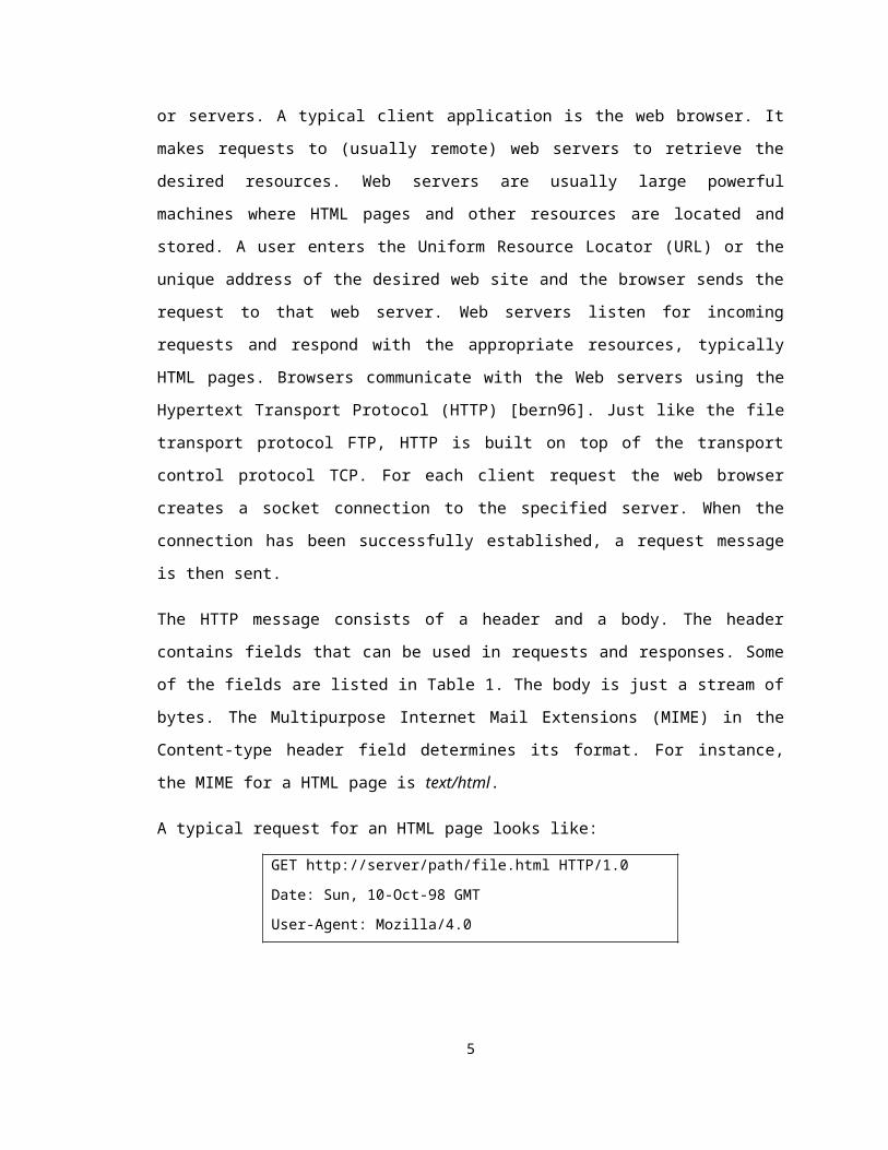
The HTTP message consists of a header and a body. The header contains fields that

can be used in requests and responses. Some of the fields are listed in Table 1. The

body is just a stream of bytes. The Multipurpose Internet Mail Extensions (MIME) in the

Content-type header field determines its format. For instance, the MIME for a HTML

page is text/html.

A typical request for an HTML page looks like:

GET http://server/path/file.html HTTP/1.0

4

Date: Sun, 10-Oct-98 GMT

User-Agent: Mozilla/4.0

The response from the web server could be:

HTTP/1.0 200 OK

Content-length: 150

Content-type: text/html

<HTML>

<HEAD><TITLE>This is the title</TITLE></HEAD>

<BODY>

<H1>

This is the content of the page.

</H1>

</BODY>

</HTML>

2.1.3 Performance

2.1.3.1 HTTP/1.0 and HTTP/1.1

The first version of the protocol for the WWW is HTTP/1.0. It is a very simple protocol. In

a typical web page, there is an HTML text and one or more images. Under HTTP/1.0, a

request is first made to the web server to retrieve the HTML page. Then a separate

connection is made to the same web server to retrieve each of the images in the HTML

page. Thus, in an HTML page with N images, N+1 connections are made, plus N+1 data

requests. Creating a TCP connection to the server imposes certain overhead. Spero

[sper94] made the first attempt to analyze the performance and summarizes the

problems of using HTTP over TCP as a transport mechanism. He found that HTTP

requests spend most of the time waiting rather than actually transferring data. Initially,

TCP establishes connections via a three-way handshake. Then the data is segmented

into smaller packets – 536 bytes per segment. In order to prevent the sender from

overflowing the receiver, TCP employs a congestion management scheme called Slow

Start. At the beginning, a window size of one is used for the sender’s unacknowledged

segments. This indicates how many segments the sender can have outstanding without

5

having to wait for any acknowledgements. When an acknowledgement is received

without loss, the window is increased. Every time a segment is lost and times out, the

window is decreased. Since the HTTP header is longer than 536 bytes, with Slow Start,

it takes 2 Round Trip Times (RTT) to make the first connection.

Clearly, having to establish a new connection for each object is not very efficient.

Netscape Communication proposed an extension to HTTP/1.0 with the ‘Keep-Alive’

header. Keep-Alive is a TCP/IP feature that keeps a connection open after the request is

complete, so that the client can quickly reuse the open connection. This mechanism

worked well except for cases where proxy servers2 were involved. Other studies

[mogu95, touc96, heid97a] have also been conducted to analyze the effects of a

persistent TCP connection for HTTP (a.k.a. P-HTTP). Persistent connection was later

incorporated into HTTP/1.1 [fiel96], the next version of the protocol.

The major changes in HTTP/1.1 are mostly related to performance. Some of the

additions in HTTP/1.1 are:

Persistent connections.

A single TCP connection can be used to request multiple objects. This is

especially efficient for an HTML page that contains several images.

Compression/decompression support.

Files can be transferred in a compressed state to improve the throughput.

Allow byte range transfer.

The ability to request a certain range of bytes from a file is extremely useful when

a transfer is interrupted. Only the remaining portion of the file needs to be

transmitted.

2 Proxy server provides a secure and efficient manner for a Local Area Network to interface with

the Internet. Since it is the only point of connection, proper security can be implemented and also

caching can be used to provide efficient retrieval of popular HTML pages. A detailed description

can be found in [naik98,pp242-245].

6

2.1.3.2 Beyond HTTP/1.1

Besides P-HTTP, there are studies for pipelining the requests [padm94, neil97] where

multiple requests are sent to the server without having to wait for acknowledgements.

This has been found to outperform HTTP/1.0. Heidemann et al. [heid97b], proposed a

model to evaluate and compare the performance of HTTP over several transport

protocols including TCP, Transaction TCP (T/TCP), UDP3-based request-response

protocol, and P-HTTP.

The next version of HTTP is currently being drafted and it is called HTTP-NG (Next

Generation) [spre98]. The working draft of HTTP-NG can be found at W3C’s web site. It

focuses not only on further performance improvements but also easier Web protocol

evolution and application developments.

2.2 Telemedicine

2.2.1 Introduction

Telemedicine is the transmission of medical information between two distributed sites. A

common scenario is the communication between clinics located in rural areas and the

general hospital in the nearby town. Patient and medical information must be retrieved

from the server machines to the remote client machines in a timely manner. Some types

of information involved are high-resolution images, live video, sounds, and other patient

records. The transmission can be made through telephone lines, ISDN, T-1, ATM,

satellites and the Internet.

Telemedicine has been an ongoing research activity for decades now but with the recent

popularity of the Internet there has been tremendous growth in this area. Some of the

earlier projects involving telemedicine are: Space Technology Applied to Rural Papago

Advanced Health Care (STARPAHC), Video Requirements for Remote Medical

Diagnosis, Massachusetts General Hospital/Logan International Airport Medical Station,

and The North-West Telemedicine Project. A good source for finding references and

articles of the different projects is the Telemedicine Information Exchange‘s (TIE)

Bibliography Database at the web site http://tie.telemed.org.

3 User Datagram Protocol is used in a connection-less transport protocol.

7

http://tie.telemed.org/

2.2.2 Imaging Aspects

2.2.2.1 Medical Imaging Techniques

The recent advances of medicine combined with new technology have resulted in a vast

array of medical imaging techniques for diagnostic purposes. There is Computed

Tomography (CT), which measures the attenuation of X-ray beams passing through the

body. Dense areas of the body absorb more X-rays and thus the measuring sensors pick

up less X-rays. CT produces images showing the human anatomy with distinct

radiographic differences between tissues of different densities such as bone, fat, and

muscle.

Magnetic Resonance Imaging (MRI), on the other hand, relies on the inherent

characteristics of atomic nuclei, usually the 1H nuclei4, in the body. The region of interest

is subjected to a strong magnetic field causing the protons to resonate. Irradiating with

radio frequency waves causes the resonating protons become excited. The radiation

emitted from the excited atomic nuclei in the region is then recorded as radio frequency

emissions. Image reconstruction is done using Fourier Transformation techniques to

convert the frequency information into spatial intensity information of the slice through

the body. This is just a brief description of the complicated procedure; a more detailed

coverage of MRI techniques can be found in [pete88].

Emission Computed Tomography (ECT) is one of the most important applications of

radioactivity in medicine. ECT measures the gamma ray flux emitted by radiotracers

such as 123I, 15O, and 13C, which have been injected into the organ of interest in the

patient. Some examples of practical applications of ECT are the investigation of cerebral

blood flow, amino acid metabolism, and the interaction between a drug and the brain.

Two important forms of ECT are Single Photon Emission Computed Tomography

(SPECT) and Positron Emission Tomography (PET).

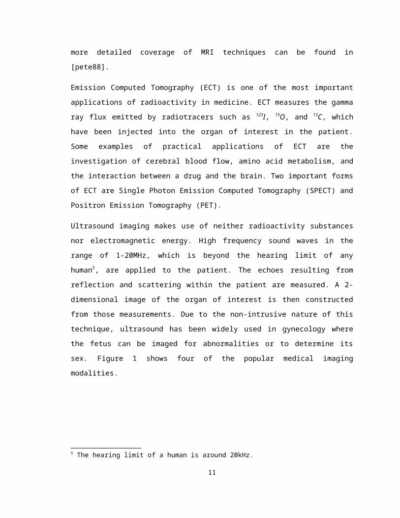
Ultrasound imaging makes use of neither radioactivity substances nor electromagnetic

energy. High frequency sound waves in the range of 1-20MHz, which is beyond the

hearing limit of any human5, are applied to the patient. The echoes resulting from

reflection and scattering within the patient are measured. A 2-dimensional image of the 4 Hydrogen nuclei have mostly been used as they are abundant throughout the body.5 The hearing limit of a human is around 20kHz.

8

organ of interest is then constructed from those measurements. Due to the non-intrusive

nature of this technique, ultrasound has been widely used in gynecology where the fetus

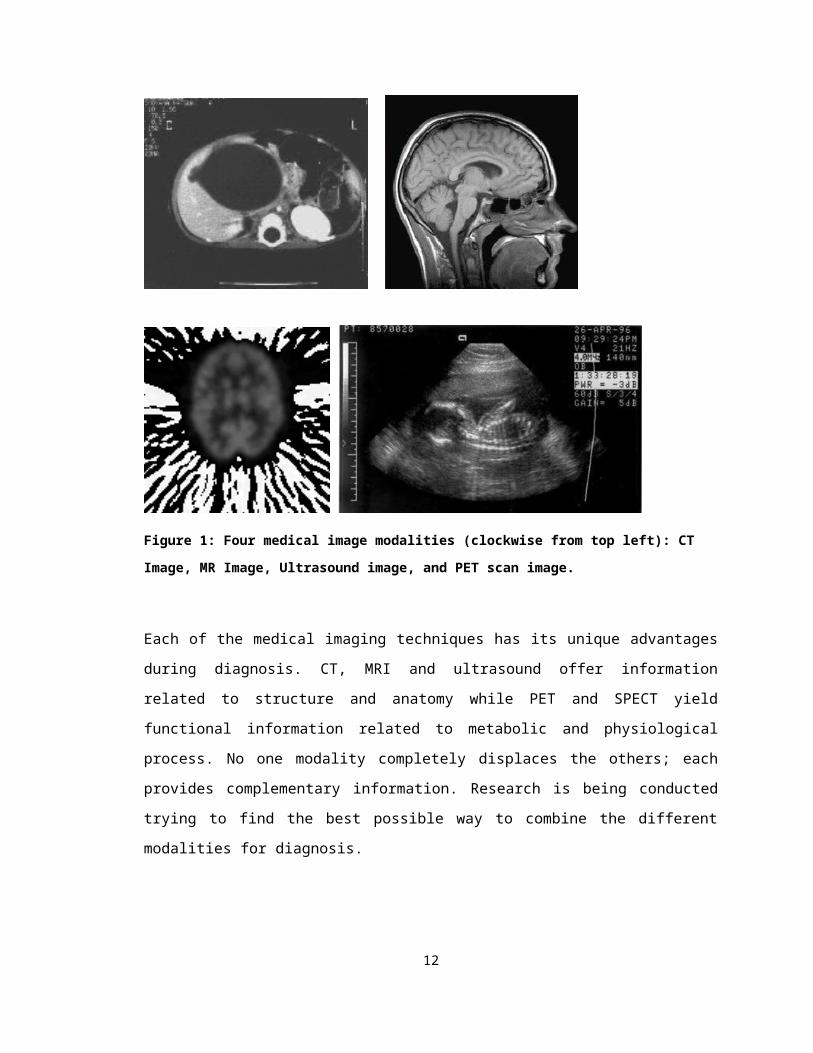
can be imaged for abnormalities or to determine its sex. Figure 1 shows four of the

popular medical imaging modalities.

Figure 1: Four medical image modalities (clockwise from top left): CT Image, MR Image, Ultrasound image, and PET scan image.

Each of the medical imaging techniques has its unique advantages during diagnosis.

CT, MRI and ultrasound offer information related to structure and anatomy while PET

and SPECT yield functional information related to metabolic and physiological process.

No one modality completely displaces the others; each provides complementary

information. Research is being conducted trying to find the best possible way to combine

the different modalities for diagnosis.

9

2.2.2.2 Teleradiology

Teleradiology involves transmitting of high-resolution medical images from one site to

another and displaying them effectively such that a radiologist can perform proper

diagnosis. Due to the characteristics of the images, there are challenges to overcome in

order to transmit these images efficiently.

Size.

An image could potentially occupy anywhere between 1MB to 8MB of storage

space, and hence require very high bandwidth to transmit in a timely manner.

However, scaling down the images might result in lost vital information.

Multiple images.

MR, and CT usually come as a set of images, called a film, which represents the

volume cross-section of an organ, slice by slice.

Images are noisy.

Medical images seem to be just made up of grayscale images surrounded by

black patches. But when they are digitized, you will find lots of noise in the

image. Noisy images do not compress well. Applying the standard lossless

compression algorithms, you can get at most 3:1 or 2:1 compression ratio. Lossy

algorithms like JPEG can be used to increase the compression ratio, but at the

same time important information is lost, which is not acceptable. Studies are

being done using wavelet compression techniques to determine what the

accepted levels of lossy compression are to achieve the highest compression

ratio while at the same time retaining all of the vital information [eric98].

2.2.3 Imaging Standards and DICOM

As more and more vendors begin to develop hardware and software to enable the

transmission of medical images, we might be faced with the problem of incompatibility.

Incompatibility happens when a display terminal from one manufacturer is not be able to

retrieve any information, or worse yet, receives incorrect information from the server that

is made by another manufacturer. It is obvious some standards have to be put in place

10

for proper and predictable transmission of vital information. The American College of

Radiology (ACR) and National Electrical Manufacturers Association (NEMA) put together

the Digital Imaging and Communications in Medicine (DICOM) standard for

manufacturers and users of interconnected medical imaging equipment on standard

networks [hori93]. The standard defines what kinds of information can be transmitted

and how information should be transmitted between two DICOM compliant devices.

11

CHAPTER 3 Magnetic Resonance Image Viewer

3.1 Introduction

Figure 2: A light-screen that radiologists use to look at MR films.

Traditionally, radiologists use light screens to display medical image films as shown in

Figure 2. For Magnetic Resonance (MR) images, a film consists of a series of image

slices laid out in a rectangular fashion. The film is placed vertically on top of the light

screen as radiologists look for anomalies. As more and more films are being taken,

storing and retrieving them efficiently and effectively has become problems. There is the

potential for misplacing patients’ files, and accessing the films at another location usually

is not immediate. With the advances in computer systems, there is the possibility of

shifting to a filmless environment. The images, which are acquired digitally, are archived

on electronic devices and displayed through computer monitors. Keeping the images as

‘soft’ digital copy makes sharing among radiologists at different locations much easier.

In a filmless environment, the images are presented only through a computer monitor,

which is much smaller in dimension compared to the traditional light screen. Displaying

12

all the images in such a limited screen area imposes certain restrictions. To solve the

problem, a different way of presenting a film of images must be used.

Van der Heyden [heyd98] in her M.Sc. thesis investigated the screen “real estate”

problem for displaying films of MR images. She implemented and then experimented

with several ways to layout the images on a single film such that those images of interest

(also called focal nodes) can be enlarged while the rest are reduced in their sizes but

remain visible on the screen to provide contextual information. The film of images is

stored locally on disk and the Image Viewer displays them in a user specified dimension.

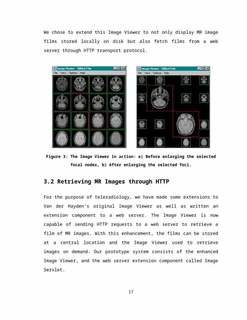
Figure 3 shows the different stages of the Image Viewer in action. Figure 3a is the initial

layout after all the MR images in the film have been downloaded and two of the images

have been selected as focal nodes6 (the two outlined in with darker border). Then Figure

3b shows that the two focal nodes are enlarged while the non-focal nodes are reduced in

sizes.

We chose to extend this Image Viewer to not only display MR image films stored locally

on disk but also fetch films from a web server through HTTP transport protocol.

Figure 3: The Image Viewer in action: a) Before enlarging the selected focal nodes, b) After enlarging the selected foci.

6 In Figure 3, the focal nodes are the ones with darker borders but they appear as red borders on

color screens.

13

3.2 Retrieving MR Images through HTTP

For the purpose of teleradiology, we have made some extensions to Van der Hayden’s

original Image Viewer as well as written an extension component to a web server. The

Image Viewer is now capable of sending HTTP requests to a web server to retrieve a

film of MR images. With this enhancement, the films can be stored at a central location

and the Image Viewer used to retrieve images on demand. Our prototype system

consists of the enhanced Image Viewer, and the web server extension component called

Image Servlet.

3.2.1 Image Viewer Enhancements

Retrieving films from the web server

Instead of just being limited to displaying MR films stored locally on disk, the Image

Viewer can now send a HTTP request to retrieve films stored on the specified web

server. The URL for the HTTP request has the following form:

http://<servername>/<path>/<filmname>. The corresponding web server responds by

sending back the film descriptor. From the film descriptor, the Image Viewer knows how

many images the film contains. Subsequent requests (one request for each of the

images) are made to the web server to retrieve the images. When all the images in the

film have been retrieved, they are displayed in their initial state, as shown in Figure 3a.

Toggle continuous enlargement

An option was added to toggle the continuous enlargement of focal nodes. In the original

Image Viewer, when a focal node is enlarged, we provide visual feedback in the form of

continuous enlargement. With the visual feedback, users can better understand how the

image transitions took place. Unfortunately, this adds overhead to the response time.

For experienced users and those that already have a good understanding of the image

layouts, a fast response time is more desirable.

Supports multiple focal nodes in a constrained area

Multiple focal nodes can now be selected in a constrained area. A constrained area is an

area that contains a subset of the images.

14

Display speed improvement

Each image is now constructed as a lightweight Java component instead of a full

component. As a full Java component, every time the size of an image changes, the

Java Virtual Machine7 issues a repaint for it. Hence, with a film typically containing

between 16 to 20 images, the repainting process takes up a huge amount of time and

this causes flickering when the focal nodes are enlarged. Since a lightweight component

is not handled by the Virtual Machine, I have removed many of the unnecessary repaint

events. With this change, we can observe a significant improvement in the response

time and eliminate the unwanted flickers.

Background color

Based on the feedback from several radiologists, we have changed the background

color of the Image Viewer to black instead of white. A darker background reduces the

contrast against MR images.

Performance Logging

From the Options menu, logging can be turned on. It logs the time to fetch a film of

images from the Image Servlet. Altogether two time components are logged in the Image

Viewer. The time components represent the time taken to retrieve and to construct the

images before they are displayed. The time components are described in detail in

Section 4.2.3.

3.2.2 Image Servlet

Image Servlet is an extension to any web server that implements the Java Servlet API8.

The API is a set of well-defined Java classes that are invoked by the web server. For our

testing purposes we have used the Java WebServer from JavaSoft. By implementing

these classes in the servlet any requests designated for the servlet are directed to it.

7 Java Virtual Machine is an application that interprets Java programs. This is the application that

makes Java programs platform independent. For further information please refer to JavaSoft

website at http://www.javasoft.com.8 The Java Servlet API can be obtained from JavaSoft’s website,

http://www.javasoft.com/products/servlet/index.html.

15

http://www.javasoft.com/products/servlet/index.html

http://www.javasoft.com/

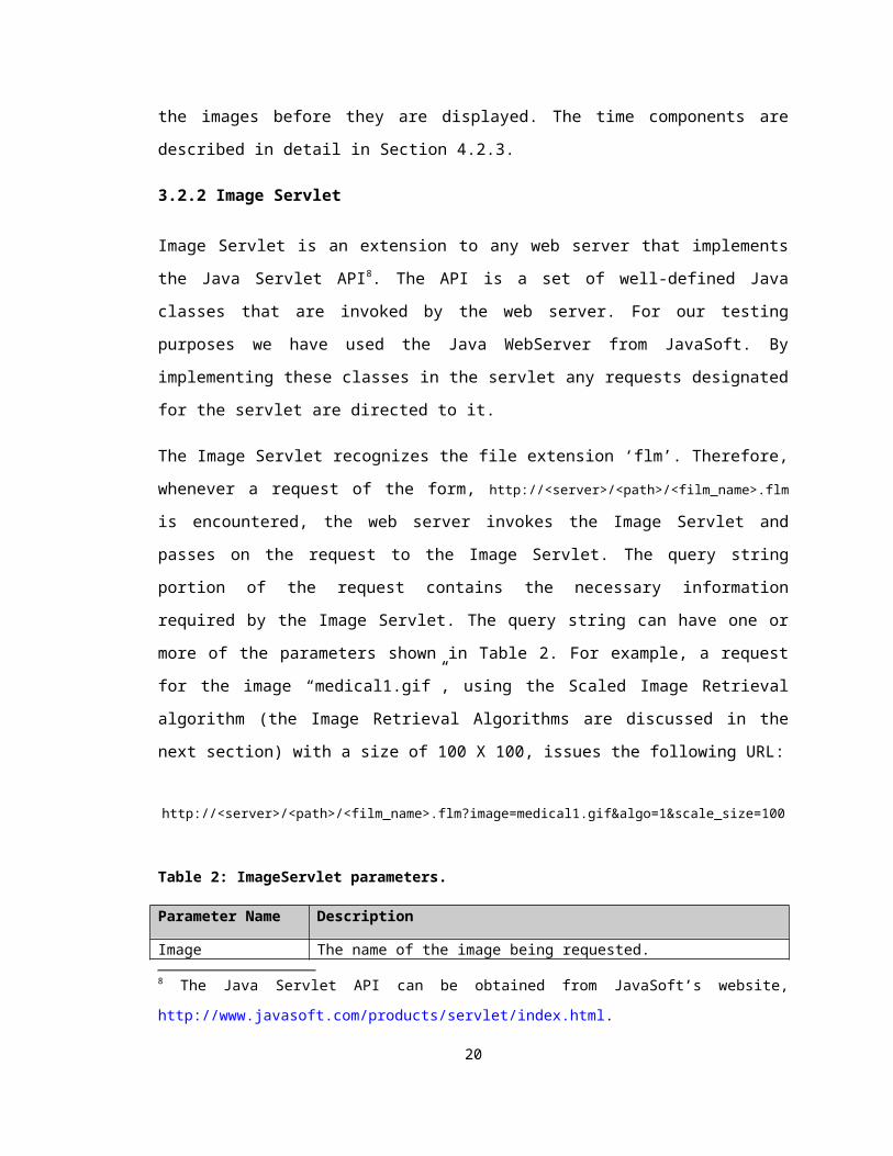
The Image Servlet recognizes the file extension ‘flm’. Therefore, whenever a request of

the form, http://<server>/<path>/<film_name>.flm is encountered, the web server

invokes the Image Servlet and passes on the request to the Image Servlet. The query

string portion of the request contains the necessary information required by the Image

Servlet. The query string can have one or more of the parameters shown in Table 2. For

example, a request for the image “medical1.gif”, using the Scaled Image Retrieval

algorithm (the Image Retrieval Algorithms are discussed in the next section) with a size

of 100 X 100, issues the following URL:

http://<server>/<path>/<film_name>.flm?image=medical1.gif&algo=1&scale_size=100

Table 2: ImageServlet parameters.

Parameter Name Description

Image The name of the image being requested.

Algo The algorithm to use when sending the image from Image Servlet.

Available algorithms are: 1) Full-resolution, 2) Scaled, and 3) Pre-

compressed. Table 3 below describes their differences.

Scale_size The size of the image to be returned. This is used in conjunction with

the Scaled algorithm.

Grayscale Whether the image is grayscale only. This optimization applies to

grayscale images only, as is the case with MR images. Since it is

grayscale, each of the Red, Blue and Green elements in the pixel has

the same value. Therefore, instead of sending 4 bytes, we can just

send one byte representing the grayscale value between 0 and 255.

16

Figure 4: Image Servlet architectural diagram.

The Image Servlet is designed to be extensible so that different image retrieval modules

can be easily added to the system. Figure 4 is a high-level architectural diagram for the

Image Servlet.

3.2.3 Image Retrieval Algorithms

There are three different Image Retrieval algorithms implemented in the prototype

system. They are Full-resolution, Scaled, and Pre-compressed. Each of the algorithms is

described in detail in the following sections and summarized in Table 3.

Full-resolution

The full-resolution algorithm retrieves full size MR images from the Image Servlet. Once

the images have been downloaded, they are stored locally in memory with the Image

Viewer. Further manipulations to these images do not result in another request. This

algorithm takes a little more time upfront but after that, it does not induce any

transmission overhead when focal nodes are being enlarged.

Scaled

One way to reduce the initial transmission overhead is to download a scaled down

version of the images. The layout size determines how much to scale the images. This

results in a quick response time to display the film. Although the images are not in their

17

full resolution, they are adequate for radiologists to distinguish one slice of the image

from another. From the study [heyd98, page 51], it is noted that each image needs to be

around 50 X 50 pixels to be distinguishable in a film.

When the radiologists need to look for anomalies or perform diagnosis on particular

images, they mark them as focal nodes. The focal nodes can be enlarged so that details

in the images can be clearly seen. With this image retrieval algorithm, every time an

image is enlarged, a request is sent to the server to fetch the full size image. Once the

full size image is retrieved, it is cached locally and further manipulations on it will have

less overhead. Therefore, even though this algorithm has a minimal initial transmission

overhead, but the overhead increases every time an image is enlarged.

Pre-compressed

With the Pre-compressed retrieval algorithm, compressed versions of the original MR

images are sent back from the Image Servlet to the Image Viewer. The images are not

compressed ‘on the fly’ but they are pre-compressed. The main objective in this

algorithm is to reduce the size of the files to transmit and at the same time eliminate the

need to make further requests when the focal nodes are being enlarged.

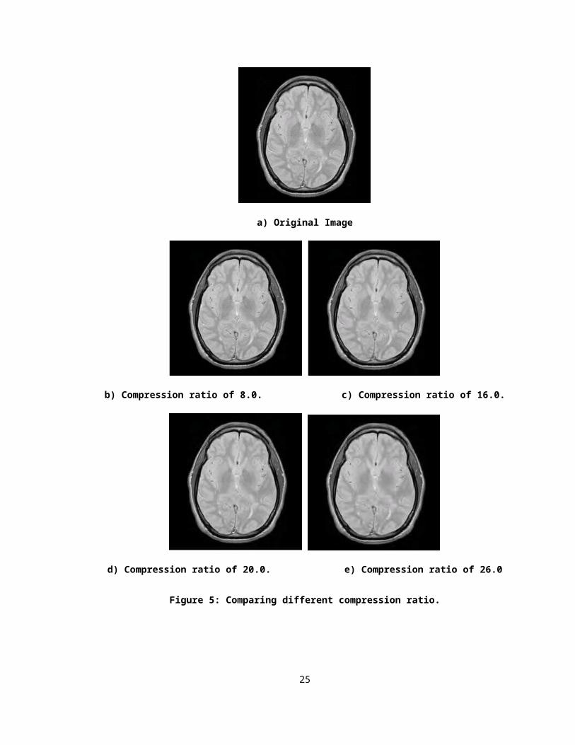
We are assuming that the compression ratio is reasonable and does not result in loss of

any vital information for diagnostic purposes. A compression ratio of 16 reduces the

original image size approximately 16 times while maintaining the majority of subtle

details in the image. This ratio was selected by visually comparing the resulting four

images compressed with a ratio of 8, 16, 20 and 26 respectively. Figure 5 presents the

four images used during the selection procedure. Figure 5a is the original full resolution

image and it is used as a comparison to the other compressed images. Once the Image

Viewer receives the compressed images, the viewer needs to decompress them to full

resolution and caches them locally.

Table 3: Image retrieval algorithm description.

Algorithm Description

Full-resolution Each image is sent in its original resolution to the viewer. Once the images

have been downloaded, they are cached locally in the viewer and no further

request to the server is needed.

18

Scaled When the display size is less then the original resolution of the image, a

scaled version of the image is requested. Image Servlet performs the

scaling (or sampling) process before sending the smaller, scaled image to

the viewer. A new request is needed to fetch the full resolution image when

it is selected as a focal image.

Pre-compressed The film of images is pre-compressed at an acceptable ratio. The viewer

requests these compressed images and performs the decompression

before displaying them. No further request to the server is necessary.

a) Original Image

b) Compression ratio of 8.0. c) Compression ratio of 16.0.

19

d) Compression ratio of 20.0. e) Compression ratio of 26.0

Figure 5: Comparing different compression ratio.

3.2.2.4 Comparing Scaled-down and Compressed Images

Figure 6: Comparing a) The original image (Top) with b) Scale-down image (Bottom left) and c) Compressed image (Bottom right).

20

Using the Scaled algorithm can be very efficient as we just download the smaller scaled

down image for display and there is no overhead with respect to decompressing the

image. But, as we are just bringing down a sample of the original image, some vital

information in the image may be lost or distorted. Thus, when the image is selected for

enlargement, we need to make a request to fetch the full resolution image. This is

necessary as we can see in Figure 6b, where a scaled down image is enlarged. We can

observe the irregularity created by enlarging the scaled down image. This is not

acceptable for diagnosis.

On the other hand, a compressed image can produce more acceptable results, as

shown in Figure 6c. There is no extra request to the server as we have compressed the

image using the full size image. No doubt there is a smoothing effect caused by the

lossy compression algorithm but if the compressed image managed to preserve all the

vital information then it is acceptable for diagnosis. There is much active research

[eric98] in this area to produce compression techniques that both achieve high

compression ratio, yet preserve the all the vital information in the images.

21

3.2.3 Process Flow

Figure 7: Process Flow Diagram.

Figure 7 shows the process flow beginning with the Image Viewer initiating the request

to the Image Servlet. First, a request of the form

http://<server>/<path>/<film_name>.flm is sent to fetch the film descriptor. A film

descriptor is a file that contains information pertaining to the film of images. Usually, the

film descriptor file is kept together with the film of images. The Image Servlet is set up to

recognize requests with the extension ‘flm’ and it sends the film descriptor file back to

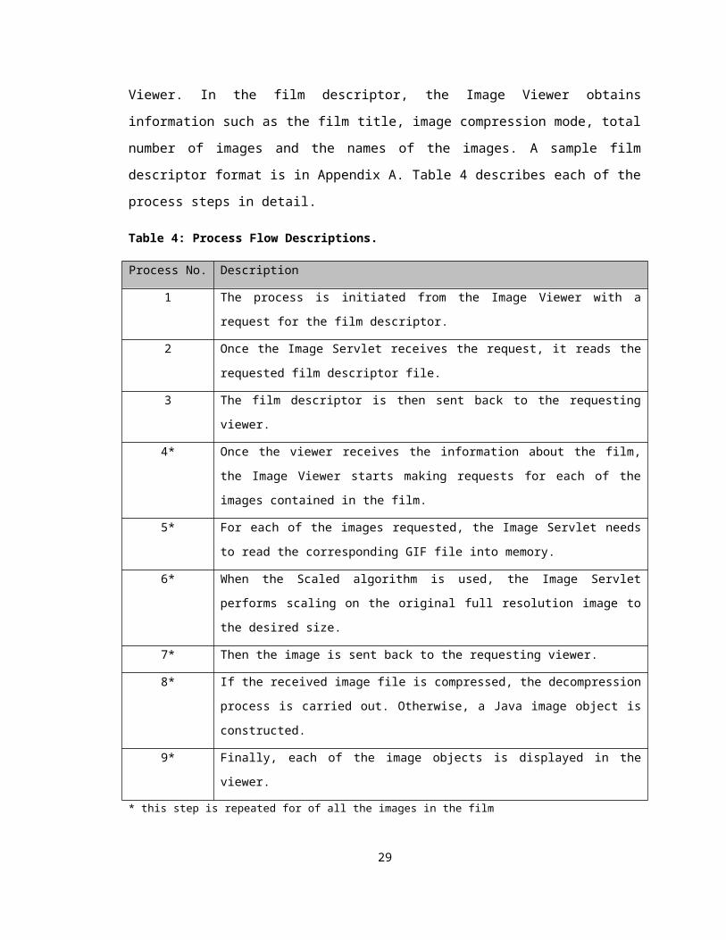
the Image Viewer. In the film descriptor, the Image Viewer obtains information such as

the film title, image compression mode, total number of images and the names of the

images. A sample film descriptor format is in Appendix A. Table 4 describes each of the

process steps in detail.

22

Table 4: Process Flow Descriptions.

Process No. Description

1 The process is initiated from the Image Viewer with a request for the film

descriptor.

2 Once the Image Servlet receives the request, it reads the requested film

descriptor file.

3 The film descriptor is then sent back to the requesting viewer.

4* Once the viewer receives the information about the film, the Image Viewer starts

making requests for each of the images contained in the film.

5* For each of the images requested, the Image Servlet needs to read the

corresponding GIF file into memory.

6* When the Scaled algorithm is used, the Image Servlet performs scaling on the

original full resolution image to the desired size.

7* Then the image is sent back to the requesting viewer.

8* If the received image file is compressed, the decompression process is carried

out. Otherwise, a Java image object is constructed.

9* Finally, each of the image objects is displayed in the viewer.

* this step is repeated for of all the images in the film

23

CHAPTER 4 Performance Evaluation

4.1 Introduction

This project investigates the feasibility of viewing MR images that are stored on a remote

web server using the HTTP protocol. We would like to provide the answer to the

following question: “Is real-time viewing of MR images feasible using a client such as

Image Viewer and a web server component like the Image Servlet?”

We have conducted experiments to determine the performance of the prototype system

under different algorithms. A good response time is especially important in client/server

applications where there is already overhead in network transmissions and protocols. A

web browser and server are such a client/server application where a reasonable

response time is crucial in order for wide acceptance and use. Therefore, many

researchers have conducted experiments on the performance of HTTP protocol as

described in Section 2.1.4. Much insight in how well HTTP is suited for transmitting web

pages have been recorded and based on these findings improvements have been made

in the later version of the protocol [fiel96, spre98]. However, our experiments were

conducted using the HTTP/1.0 protocol, as it is still the widely used version.

Before we describe the experiment design, there are a number of pitfalls that we should

be aware of and try to avoid during the experimental runs. They are suggested in

[tane96a] for measuring network performance and are presented here for our

experiments.

Make sure that the sample size is large enough and representative.

In general a large number of samples reduce the percentage of uncertainty in a

measurement. But for our experiments, the standard deviation was less than 10% of the

mean for the Full-resolution algorithm and less than 5% for Scaled and Pre-compressed

algorithms. We felt that for this particular situation 10 experimental run is acceptable.

24

Be careful when using a coarse-grained clock.

Most computer timers have a granularity of a millisecond. So every ‘tick’ adds one

millisecond to the timer. If we were to measure an activity that takes time T, in which T is

not an integral of a millisecond, then we have introduced error into the calculation. One

solution to this problem is to use a finer-grained clock, but if this is not possible, then we

should take a large number of measurements to reduce the error9.

In our experiments, the film we use is consists of 16 MR images and we make sure that

the sample size is large and representative.

Be sure that nothing unexpected is going on during the test.

Unless both client and server applications are running on a dedicated network, it is

difficult to prevent processes from utilizing the network. What we have done is to perform

the experimental runs at night where network activity is low. We can observe from the

data collected there are no outliers and only occasional small fluctuations.

Caching can wreck havoc with measurements.

In order to avoid using cached images in the viewer, after each run of the experiment,

the Image Viewer was shutdown completely and a new instance was started for the next

experimental run.

Understand what you are measuring.

Some of the factors that might affect the measurement are: the operating system in the

client and server machine, the network used, image characteristics, and the image

retrieval algorithm used. All of these were kept constant except for the algorithm used.

Thus we obtain a valid comparison of the performance of the different image retrieval

algorithms.

4.2 Experiment Design

9 Even with a large number of samples, the error will not be reduced to less than 0.5 millisecond

due to roundups in the measurement.

25

4.2.1 Objective

In section 3.2.3 we described three image retrieval algorithms that can be used from the

Image Viewer to retrieve a film of MR images from a web server. The algorithms are

Full-resolution, Scaled, and Pre-compressed. In order to determine how each of the

algorithms behave and perform, we conducted experiments on them. From the data

collected, we have come to a conclusion as to which of the three algorithms is more

suitable for real-time MR image viewing. This is discussed in the next chapter.

4.2.2 Experiment Setup

The Image Viewer and Image Servlet are designed to work across the Internet. The

viewer is implemented to use the standard HTTP/1.0 protocol to communicate with the

server. Since this thesis serves as a preliminary investigation, we used a controlled

network environment in the School of Computing Science instead of conducting the

experiment on the Internet. In such an Intranet environment, we have limited the amount

of congestion that is normally encountered in the Internet. Two identical machines were

used, connected over an Ethernet. One machine was running the web server with the

Image Servlet component while the Image Viewer ran on the other. A film of 16 MR

images was used in the experiments. Each of the images has a typical size of 256 X 256

pixels10. Table 5 lists the rest of the settings for the experiments.

Initially all the images are stored in the web server machine. We assume that the server

machine caches some or all of the MR images in memory. In this particular experiment,

the assumption that the images came from a warm cache is acceptable, as our purpose

is not to compare disk access times against memory access times. Also, with the

existence of network transmission and image processing overhead, disk access time is

considered insignificant. Nevertheless, in order to have consistent data, the first runs of

the experiments were discarded so that disk access and other initialization times were

not included in the analysis.

Table 5: Experimental Setups.

Operating System WindowsNT 4.0 Workstation

10 Typical resolution for MR images is 256 X 256 pixels.

26

Simon Tang, 01/03/-1,

Newly added

CPU Pentium 166MHz

Memory (RAM) 32 MB

Network Ethernet (1Mbps)

# of images in film 16 (layout 4 X 4)

Image resolution (in pixels) 256 X 256

Average Image Size (as GIF) 44,364 bytes

Depending on the image retrieval algorithm selected, the total number of bits transmitted

from web server to Image Viewer differs. With the Full-resolution algorithm, the image in

its original size is retrieved and this results in a large number of bits to be transmitted

when compared to the Scaled algorithm. In Table 6 we present the number of bits

associated with the three algorithms and also the theoretical transmission time using an

Ethernet, a T1 line, and an ATM connection.

Table 6: Theoretical Transmission Time for the Three Image Retrieval Algorithms.

Algorithms #bits/image #bits/film Theoretical Transmission Time (in ms)

Ethernet

(10 Mbps)

T1

(1.544Mbps)

ATM

(155.5 Mbps)

Full-resolution 65536 1048576 105 680 6

Scaled 19600 313600 31 203 ~0

Pre-compressed 4096 65536 7 42 ~0

4.2.3 Time Components

In order to determine which of the three algorithms is most efficient and achieves the

best performance, we calculate the total amount of time needed to retrieve a film of MR

images as well as the time to perform a set of operations with them. The time we are

measuring can be broken down into several smaller components. The following formula

can be used when calculating the total time between requesting a film of images and

displaying them:

27

where:

= Image Servlet processing and transmitting time per image

= HTTP and other overhead per image

= Image construction time in Image Viewer per image

= Total number of images in the film for the initialization stage

There are three time components associated with every request for an image. First,

there is the HTTP overhead, , which is associated with the sending of a request to the

Image Servlet and also the latency time of sending an image from the server to the

Image Viewer. Overhead in HTTP protocol includes marshalling and unmarshalling of

message headers.

Then, when the Image Servlet receives the request, it needs to read in the particular

image from disk if it is not already in memory and this involves disk latency time. In some

cases, the servlet needs to perform additional processing on the requested image before

sending it back to the Image Viewer. One such process is to scale the original image

down to the desired size for the Scaled algorithm. This overhead is denoted by .

Finally, when the Image Viewer receives the image, the viewer needs to construct the

bits received into a Java image object before the image can be displayed. If the image

retrieved is compressed, then an extra step to decompress the image is required. The

amount of time it takes to construct the Java image object is .

Once all the images have been downloaded, a set of operations is performed on them.

Since we are measuring the efficiency of retrieving images from a remote web server

and the only operation that could generate a request is enlarging the selected focal

nodes, we have measured the extra time it takes when enlarging one, two and three

focal nodes. For the different algorithms the total time may be comprised of different

portions of the above time components.

28

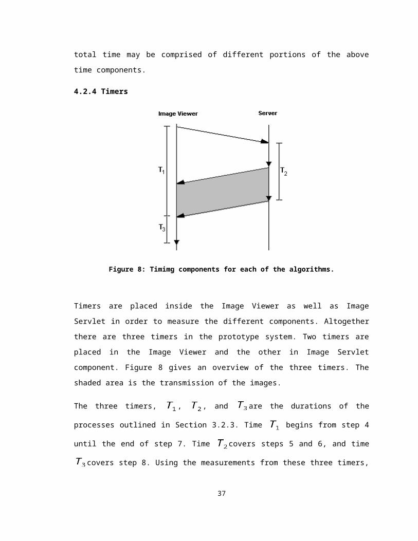
4.2.4 Timers

Figure 8: Timimg components for each of the algorithms.

Timers are placed inside the Image Viewer as well as Image Servlet in order to measure

the different components. Altogether there are three timers in the prototype system. Two

timers are placed in the Image Viewer and the other in Image Servlet component. Figure

8 gives an overview of the three timers. The shaded area is the transmission of the

images.

The three timers, , , and are the durations of the processes outlined in Section

3.2.3. Time begins from step 4 until the end of step 7. Time covers steps 5 and 6,

and time covers step 8. Using the measurements from these three timers, the above-

mentioned time components can be obtained using the following formulae:

=

= –

=

29

CHAPTER 5 Results and Discussions

5.1 End to End Observations

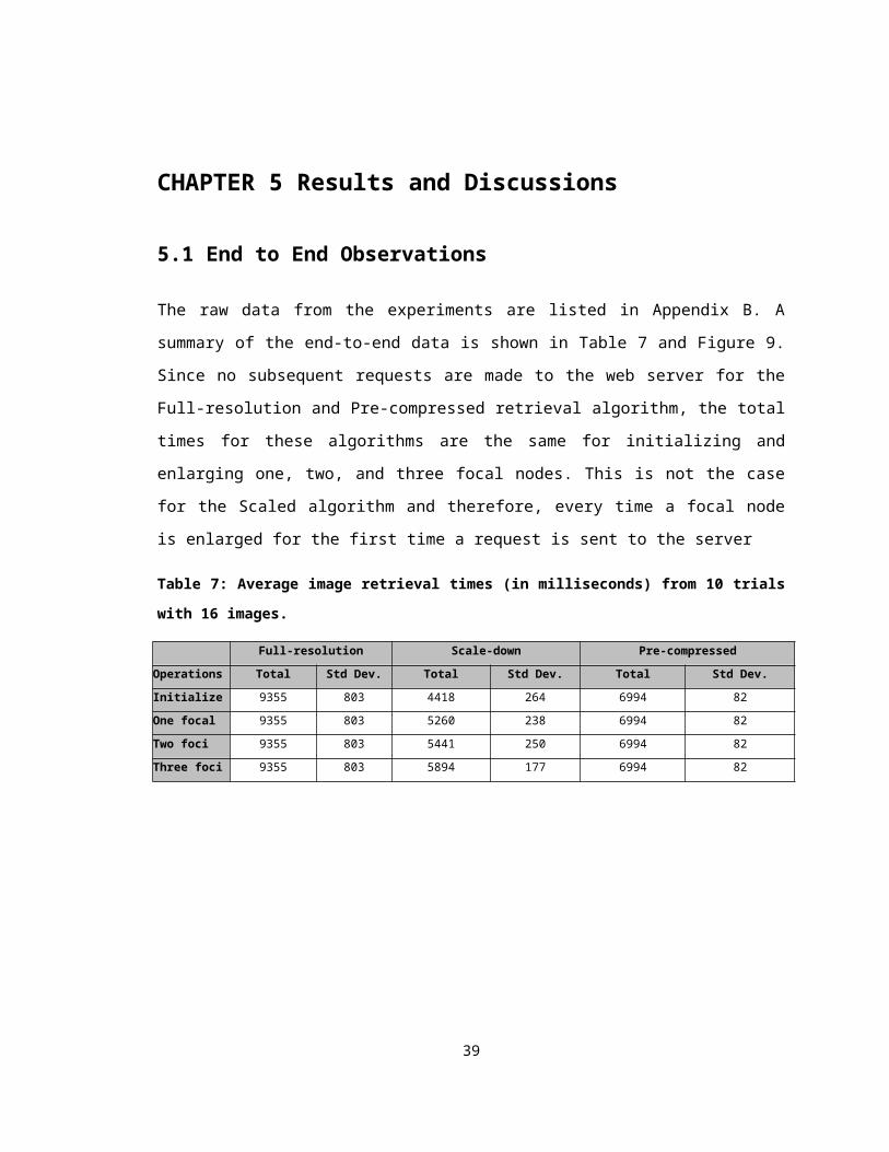
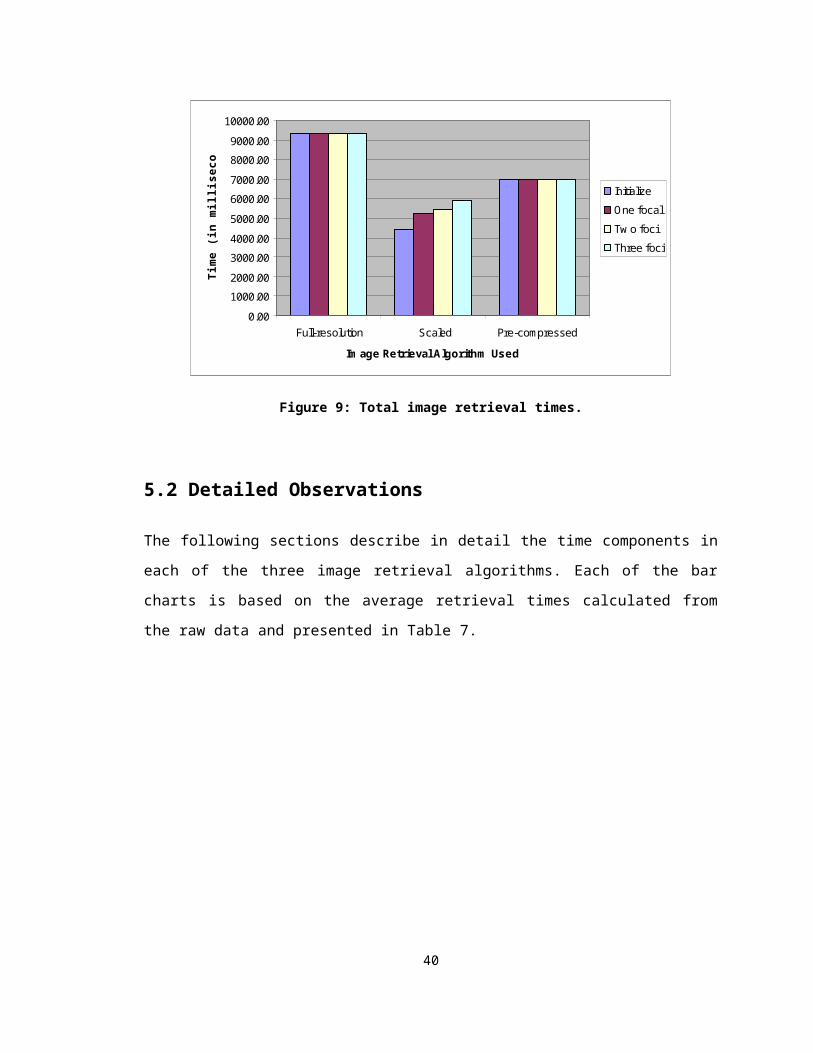
The raw data from the experiments are listed in Appendix B. A summary of the end-to-

end data is shown in Table 7 and Figure 9. Since no subsequent requests are made to

the web server for the Full-resolution and Pre-compressed retrieval algorithm, the total

times for these algorithms are the same for initializing and enlarging one, two, and three

focal nodes. This is not the case for the Scaled algorithm and therefore, every time a

focal node is enlarged for the first time a request is sent to the server

Table 7: Average image retrieval times (in milliseconds) from 10 trials with 16 images.

Full-resolution Scale-down Pre-compressed

Operations Total Std Dev. Total Std Dev. Total Std Dev.

Initialize 9355 803 4418 264 6994 82

One focal 9355 803 5260 238 6994 82

Two foci 9355 803 5441 250 6994 82

Three foci 9355 803 5894 177 6994 82

0.00

1000.00

2000.00

3000.00

4000.00

5000.00

6000.00

7000.00

8000.00

9000.00

10000.00

Full-resolution Scaled Pre-compressed

Image Retrieval Algorithm Used

Tim

e (in

mill

isec

onds

)

Initialize

One focal

Tw o foci

Three foci

Figure 9: Total image retrieval times.

30

5.2 Detailed Observations

The following sections describe in detail the time components in each of the three image

retrieval algorithms. Each of the bar charts is based on the average retrieval times

calculated from the raw data and presented in Table 7.

5.2.1 Observations for Full-resolution Image Retrieval Algorithm

Figure 10: Full-resolution Algorithm Time Components.

Retrieving all the images in the film in full size takes the longest initial time, as the

amount of time needed is proportional to the total number of bits transmitted. Hence, in

Figure 10, the server processing and transmission time, makes up most of the total

time. The Image Servlet processing time is very large because it has to read the full size

images from disk and then send them to the Image Viewer. The dotted line denotes the

theoretical transmission time over the Ethernet. It is the best case time for fetching the

film of images assuming that there are no collisions on the Ethernet and both client and

server applications do not have any processing overhead.

31

5.2.2 Observations for Scaled Image Retrieval Algorithm

Scaled Time Components

0

1000

2000

3000

4000

5000

6000

7000

Initialize 1 Focal 2 Foci 3 Foci

Tim

e (in

ms)

Image ConstructionHTTP Overheads

Server Processes

Figure 11: Scaled Algorithm Time Components.

This algorithm retrieves a scaled down version of the images and this reduces the

number of bits to be transmitted. Comparing its server processing time, , with the one

from Full-resolution algorithm, we observe that reducing the number of bits to be

transmitted has a huge effect on the total end-to-end time. In our experiments, the

images were scaled down to 140 X 140 pixels, approximately one third the size of a full

resolution image. Hence, the initial time taken is much less. The amount of time taken by

HTTP overhead, , is fairly close to that of the previous algorithm. This is expected as

these two image retrieval algorithms use very similar requesting/responding messages.

The image construction time, , could not be seen in here as it only takes up a very

small amount of the total time. The dotted line denotes the theoretical transmission time

over the Ethernet. It is the minimal time for this set of operations again assuming that

there are no collisions on the Ethernet and both client and server applications do not

have any processing overhead.

32

5.2.3 Observations for Pre-compressed Image Retrieval Algorithm

Pre-compressed Time Components

0

1000

2000

3000

4000

5000

6000

7000

8000Ti

me

(in m

s)

Image Construction

HTTP OverheadsServer Processes

Figure 12: Pre-compressed Algorithm Time Components.

The compression time is not taken into account here as the images are assumed to be

compressed elsewhere. The end-to-end time is more than for the Scaled algorithm but

less than using the Full-resolution algorithm. From Figure 12, we observe that the server

processing time, , is very small. This is because the size of the images has been

reduced by the compression. Table 6 indicates that this algorithm transmits the least

number of bits.

About 85% of the total time was used for decompressing the images at the Image

Viewer. Thus, this algorithm has the highest values among the three algorithms. The

amount of time caused by HTTP overhead, , stayed fairly consistent when compared

with the previous algorithms.

33


Why?

5.3 Did We Achieve Real-Time MR Image Viewing?

Our main objective in this thesis is to determine whether real-time viewing of MR images

across the Internet is achievable. We have conducted experiments using different image

retrieval algorithms and presented their results and observations in the previous

sections. Before we delve into the observations let us first take a look at what is meant

by real-time in such an application as the Image Viewer. Let us use the notion of frames

per second (fps) in animation as the place to begin our discussion. Animation, either

traditional or computer generated, gives the audience an illusion of motion. The

character in the animation, for example, could be walking, running, or jumping. This is

accomplished by showing the audience each of the frames at a rate of 1/24 th of a

second. The brain has the ability to remember each of the images for a very short time

and at 24 frames per second it is enough to provide us with a sense of continuous

motion. One usually calls this real-time. Cook [cook90] indicated that with just 12 fps it is

sufficient for us to perceive a continuous motion11. At anything less than this minimum

rate, it will result in a very jerky motion and is irritating to watch. Thus, the rate of 12 fps

can be called the tolerable rate.

In an application that retrieves and displays medical images, one cannot apply the rate

of 24 fps as it is not trying to produce any motion effects. The real-time here is to be able

to display the requests film of images as fast as possible. Again, this notion of ‘fast’ is

subjective and no one number can be associated to it. Therefore, we think that using the

tolerable time is more appropriate for our experiment than real-time. We can then define

tolerable time as the time the users are willing to wait before getting the results. From an

informal discussion with radiologists we came up with 3 seconds to be a reasonable

tolerable time for retrieving and displaying a film of 16 images.

11 This is only true for films without sound, otherwise the rate has to be higher in order to perceive

a continuous motion.

34

Figure 13: Components that were used in the prototype system.

Table 7 summarized the results from our experiments. Although we were not within the

tolerable time of 3 seconds, we believe that by reducing overhead throughout the system

it is achievable. Let us now look at all the components in the prototype system that could

have contributed to the overhead. The diagram in Figure 13 breaks down the major

components. In the client, the Image Viewer is an application written in Java that

requires a Java Virtual Machine12 to execute it. The lowest layer consists of the

operating system, which in our case is Windows NT. On the server-side, there’s a Java

servlet component, the Image Servlet that must be executed within the environment of

Java WebServer. Since the Java WebServer is also a Java application, it too needs the

Java Virtual Machine. The server machine also has Windows NT as the operating

system. Both client and server machine were connected on an Ethernet and the protocol

used is HTTP/1.0. As we can observe, there are many components involved besides the

network and each one of them contributes to the measured round trip time (RTT).

5.3.1 Factors Contributing to the RTT

Operating System

The overhead from the operating system involves time consuming activities such as

accessing files from disk and memory management issues. Since we have set up the

experiment such that the Image Servlet used warm cache, disk I/O would not have been

a factor but virtual memory page swapping could have been one of the factors

contributing to the server processing time. The other potential factor was context

12 Java Virtual Machine is an application that interprets Java programs. This is the application that

makes Java programs platform independent. For further information please refer to JavaSoft

website at http://www.javasoft.com.

35

http://www.javasoft.com/

switching among the processing threads. As the operating system is capable of

multitasking and there might have been system services13 running in the background,

the main thread in Image Servlet might have been context switched out. Since we have

taken into account the non-active time, the RTT could be affected.

Java Virtual Machine

Java has been known to be a platform independent language and has the goal of “Write

once, run anywhere”. In order to achieve this, a Java program, when compiled, produces

a set of Java byte codes, known as Java Class files. These byte codes cannot be

executed natively to the operating system (OS) but requires a Java Virtual Machine to

interpret them. Therefore, as long as a particular platform has a Java Virtual Machine

installed, it can run any Java programs. Unfortunately, the requirement of a virtual

machine causes additional overhead. It is known that Java programs do not perform as

well when compared to similar C++ programs that have been compiled into native

binaries.

There are many benchmark tests to compare Java programs with similar C++ programs

and [bolin97], in particular, conducted more than 30 tests to compare the performance of

Java with C++. Each test compares a low-level language construct, for example, the if-

then-else flow control. He concluded that C++ programs on average outperform Java

programs by 57%. This number is also dependent upon the nature of the program as

one program might use one language construct more then the others. Both the Image

Viewer and Image Servlet execute many repetitive loops when retrieving a film of

images and based on the “Loop overhead” reported in [bolin97], Java is more than 10

times slower than a corresponding C++ program.

Although we are aware of the overhead in the Java virtual machine, we did not have

sufficient time to re-implement the existing Image Viewer in C++ and decided to follow

the process of extending and evolving the current implementation.

13 Windows NT operating system calls applications that run in the background a service. On UNIX

it is call a daemon.

36

Java WebServer

Java WebServer can extend its processing capabilities with Java Servlet components.

Each servlet component is a specialized processing module that is plugged-into the web

server. The Image Servlet is such a component that specializes in transmitting MR

images to Image Viewer. All the requests are first received by the Java WebServer,

which then delegates them to the appropriate servlet component to be processed.

Having this extra level of indirection introduces overhead in our experiments as there

were at least 16 requests made to fetch a film of images.

Image Viewer and Servlet

The current implementation of the Image Viewer uses HTTP/1.0. As we have discussed

in Chapter 2, this protocol creates and destroys the connection for each of the requests.

Since there is overhead associated with the creation of a connection, this is further

magnified with 16 requests as in our experiments. By just implementing the HTTP/1.1

protocol there will be an immediate gain in performance.

Besides the protocol overhead, a certain portion of Image Viewer’s time is used in re-

constructing the retrieved image. This is especially significant for the Pre-compressed

algorithm where decompression is required. Huge improvements in the overall

performance can be obtained when the decompression process is reduced.

Experiments

Besides the overhead caused by the different components, there might be some delays

introduced during the experiments. Activities such as mouse movements, switching

focus to another window, and executing another application could potentially cause

unusually large time variations in the data. This is not an error in the experimental design

but in fact more accurately reflects the nature of the application. In most cases, it is very

likely that when a person uses an application, he/she will move the mouse, or switch to

another window.

37

5.3.2 Which Algorithm is Better?

Full-resolution vs. Scaled

The total time taken is proportional to the total number of bits required to download,

which is also proportional to the number of images in the film. Since the Full-resolution

algorithm retrieves the image in its original size, it needs to transmit the most number of

bits and hence it takes the longest time. On the other hand, the Scaled algorithm initially

only retrieves a sample of the original image and it takes much less time compared to

the Full-resolution algorithm. But each time a focal image is enlarged, it needs to send a

new request to the server to retrieve the full size image and this adds to the total time.

Figure 11 shows the total time taken for enlarging one, two and three image focal nodes.

The downloading time increases with the number of focal nodes enlarged. When we

extrapolate the data, the Scaled algorithm eventually performs at a rate worse than that

of Full-resolution algorithm. Then it becomes more efficient to download all the full size

images at the beginning.

On the other hand, radiologists usually focus on only a few images in a film [heyd98] and

it is sufficient to bring down a sample for the remainder of the images. In this case, the

Scaled algorithm would provide the best turnaround time. Assuming that a C++ program

is twice as efficient as a Java program, just by implementing the Image Viewer and

Image Servlet components we should be able to achieve approximately 3 seconds RTT

for retrieving a film of 16 images with two focal nodes enlarged using the Scaled

algorithm (based on the number from the experiments).

Scaled vs. Pre-compressed

Depending on the compression technique used, the Pre-compressed algorithm might be

the most efficient solution, particularly when used over the Internet. The compressed

images have the smallest size. According to the experiments conducted, this results in

the least amount of time spent in server-side processing. Having the ability to fulfill a

request quickly, the server can move on to other incoming requests. This improves the

performance when multiple Image Viewers are connected to the server, as the

decompression process is off-loaded to the client machines. The Full-resolution and

Scaled algorithm in contrast are server processing intensive and they will not perform

38


Newly added: The multiple clients connecting to a single server.

well when there are a large number of Image Viewers simultaneously sending requests

to the server.

Assuming that the compression technique is able to preserve all the vital information in

the image diagnosis, once the images have been downloaded to the Image Viewer and

decompressed, no extra requests to the server are required. Hence, the total retrieval

time remains constant. We observe from Figure 9 that the initial download and

decompression time for the Pre-compressed algorithm is much larger than the

processing time for the Scaled algorithm. However, the former does not require further

communication with the server, so as the number of focal nodes increases, the overall

time remains constant with Pre-compressed algorithm. Therefore, the Pre-compressed

algorithm is the most suitable algorithm except when only one or two focal nodes are

chosen. Since most of the computations involved (e.g., image manipulation and

decompression) are CPU intensive, by using a more powerful and faster CPU, we can

reduce the overall round trip time. The reduced time might even be within the tolerable

time of 3 seconds. Therefore, we believe that the Pre-compressed algorithm would be

the ideal solution for viewing remote MR images over Intranet and Internet.

39

CHAPTER 6 Conclusion and Summary

6.1 Conclusion

This thesis began as a project to extend the original Java-based magnetic resonance

(MR) Image Viewer [heyd98] for remote viewing. The original Image Viewer was

developed to solve the screen “real estate” problem while displaying a film of MR images

from the local file system. With the extension, the Image Viewer has the ability to request

a film of MR images that is stored remotely at a server. Three different image retrieval

algorithms have been implemented and compared. They are the Full-resolution, Scaled,

and Pre-compressed images retrieval algorithms.

Experiments were set up to measure the performance of the three image retrieval

algorithms. The total round trip time (RTT) to retrieve and display a film of images is the

main measurement of interest. By comparing the RTT taken by the three image retrieval

algorithms we came to the following conclusions:

The Full-resolution algorithm downloads all the MR images

in their full size and thus it has a large initialization time. There is almost

no reason to do so as most of the time radiologists are only interested in

a small number of the images.

Recognizing the overhead of the Full-resolution algorithm,

the Scaled algorithm only requests and downloads a sample of the

original image, large enough for the radiologists to distinguish one image

from another. This reduces the initialization time and as long as only a

small percentage of the images are of interest, this algorithm performs

best and is suitable for real-time diagnosis use.

Finally there is the use of compressed images in the Pre-

compressed algorithm. The images have to be compressed and archived

in the server machine. When the compressed image is downloaded to the

viewer, it is then decompressed before displayed. Since the compressed

40

images are very small, it only takes a fraction of the total retrieval time for

a full size image. In our experiments, the decompression process took

most of the time but with active research in compression/decompression

technology, this algorithm could be improved and it would be the ideal

solution to achieve tolerable time response in viewing MR images for

teleradiology.

6.2 Future Research

Future work involves experimenting with different image retrieval algorithms especially

applying different image compression techniques. Discovering the compression

technique that both produces a high compression ratio and maintains diagnostic

accuracy is an important milestone in the teleradiology field.

Although the performance of the Image Viewer has been increased, there are still a

number of places where it could further be improved. One such place is to experiment

with pipelining the requests (as in HTTP/1.1) to achieve the maximum throughput. While

waiting for the response for the first request, the following request can be sent to the

server.

Due to time constraints we only ran the experiments over the Ethernet. It would be a

good comparison to run a similar experiment over an ATM, T1 line, ISDN network, and

also through a 56kbps modem.

Table 8: Comparisons between Java interpreter and JIT compiler.

Matrix inversion (in sec) Matrix multiplication (in sec)

Matrix Size 50 100 150 200 50 100 150 200

Com

pile

r/run

time

MS VC++ 4.0 0.88 2.97 8.57 20.49 0.16 1.2 4.34 12.36

MS J++/MS Jview (JIT)

0.33 2.31 6.7 15.65 0.16 0.88 3.18 9.61

Cafe/Cafe Java (JIT)

0.55 3.24 10 23.07 0.22 1.37 4.99 14.28

Sun Javac/ Sun Java

4.51 32.03 N/A N/A 1.86 15.1 N/A N/A

41

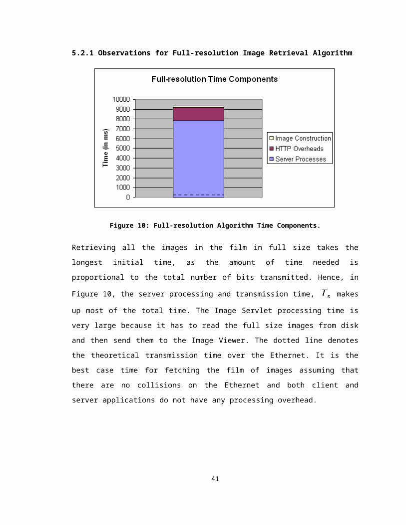
Source: Comparison work done by Intergalatic Reality. (http://www.intergalact.com/)

Section 5.3.1 discussed the performance issues of the interpretive Java programs

compared to the compiled more efficient of C++ programs. Since then there have been

commercial products called Just-In-Time (JIT) compilers for Java. The idea of JIT is to

compile the byte codes downloaded before executing them. Table 8 shows the

improvement gained when JIT compiler is used. Either re-implementing the prototype

system in C++ or makes use of the JIT compiler would be the next logical step.

42

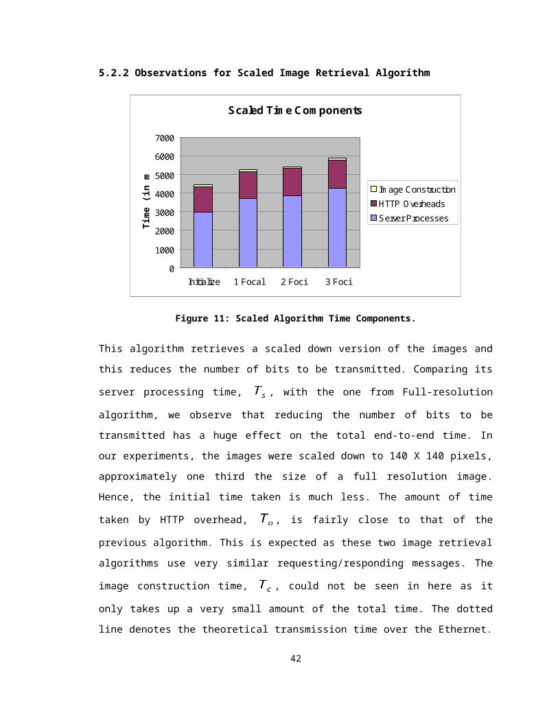
REFERENCES

[bern96] Berners-Lee T., Fielding R., Frystyk H.: "Informational RFC 1945 – Hypertext

Transfer Protocol – HTTP/1.0," MIT/LCS, UC Irvine, May 1996.

[bolin97] Bolin, R. L.: “Java Optimization and Performance”, Course project, Georgia

State University, May 1997. http://www.mindspring.com/~rlb/csc882/.

[cook90] Cook, D. A.: A history of narrative film 2nd Edition, p2 W.W. Norton & Company

Inc. New York, 1990 ISBN: 0-393-95553-2

[eric98] Erickson B. J. et al.: “Wavelet Compression of Medical Images,” Radiology,

1998, pp. 599-607.

[fiel96] Fielding R., Gettys J., Mogul J.C., Frystyk H., Berners-Lee T.: "RFC 2068 -

Hypertext Transfer Protocol -- HTTP/1.1," UC Irvine, Digital Equipment Corporation, MIT,

June 1996.

[heid97a] Heidemann J.: “Performance Interactions Between P-HTTP and TCP

Implementations,” in ACM Computer Communication Review, April 1997.

[heid97b] Heidemann J., Obraczka K. and Touch J.: “Modeling the Performance of

HTTP Over Serveral Transport Protocols,” in IEEE/ACM Transactions on Networking,

June 1997.

[heyd98] van der Heyden J.: Magnetic Resonance Image Viewing and the “Screen Real

Estate” Problem, MSc. Thesis, SFU, 1998.

[hori93] Horiil S. C., Prior F. W., Bidgood Jr. W. D., Parisot C. and Claeys G.: DICOM:

An Introduction to the Standards, 1993.

http://www.xray.hmc.psu.edu/dicom/dicom_intro/DICOMIntro.html

[mogu93] Mogul J. C.: “IP Network Performance,” in Internet System Handbook, Lynch,

D.C. and Rose, M.T. (eds), Reading, MA: Addison-Wesley, 1993, pp. 575-675.

43

http://www.xray.hmc.psu.edu/dicom/dicom_intro/DICOMIntro.html

http://info.internet.isi.edu:80/in-notes/rfc/files/rfc2068.txt

http://info.internet.isi.edu:80/in-notes/rfc/files/rfc2068.txt

http://www.mindspring.com/~rlb/csc882/

http://info.internet.isi.edu/in-notes/rfc/files/rfc1945.txt

http://info.internet.isi.edu/in-notes/rfc/files/rfc1945.txt

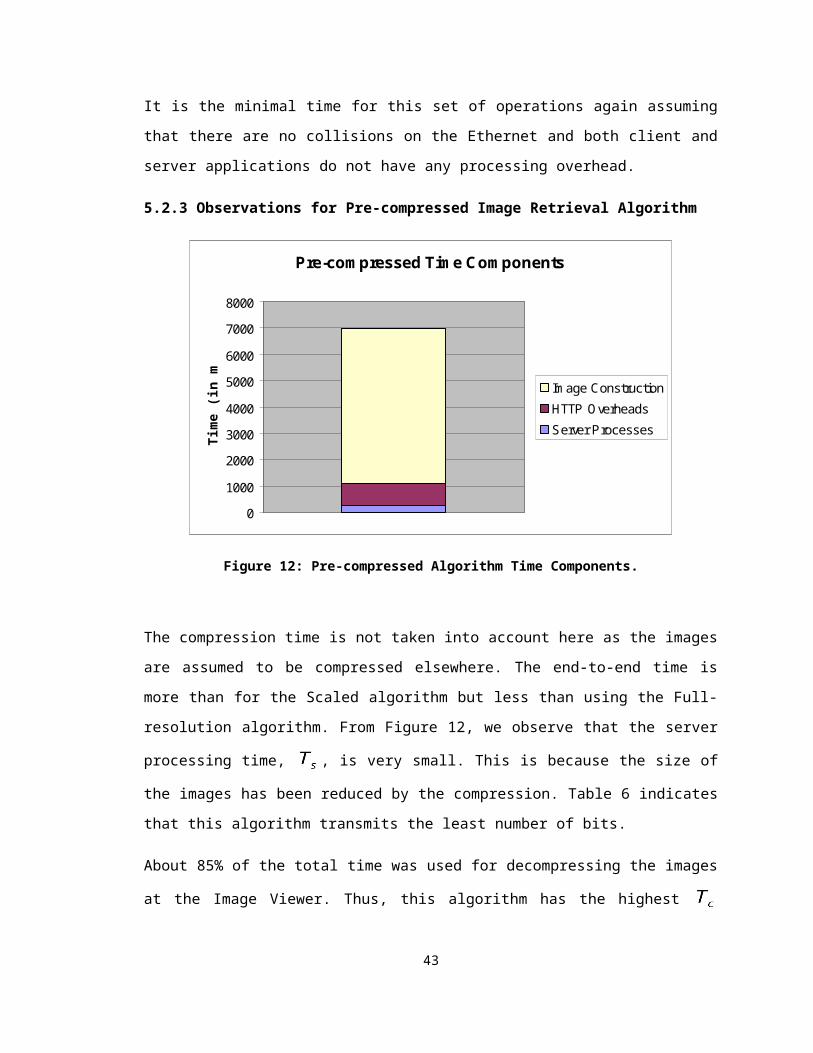
[mogu95] Mogul J. C.: “The Case for Persistent-Connection HTTP,” in Proceedings of

the SIGCOMM ’95, May 1995.

[naik98] Naik D. C.: Internet Standards and Protocols, Microsoft Press, 1998.

[neil97] Neilsen H. F., Gettys J., Baird-Smith A., Prud’hommeaux E., Wium H., and Lilley

C.: “Network Performance Effects of HTTP/1.1, CSS1, and PNG,” in ACM SIGCOMM

’97, June 1997, http://www.w3.org/Protocols/HTTP/Performance/Pipeline.html

[padm94] Padmanabhan V. N., and Mogul J. C.: “Improving HTTP Latency,” October

1994, http://www.ncsa.uiuc.edu/SDG/IT94/Proceedings/Dday/mogul/HTTPLatency.html

[pete88] Peters T. M.: “Principles and Applications of Magnetic Resonance Imaging

(MRI) in Neurology and Neurosurgery,” The Journal of Mind and Behavior, Summer

1988, Volume 9, Number 3, pp. 241-262.

[sper94] Spero S. E.: “Analysis of HTTP Performance problems,” July 1994,

http://www.w3.org/Protocols/HTTP/1.0/HTTPPerformance.html.

[spre98] Spreitzer M., and Nielsen H. F.: “Short- and Long-Term Goals for the HTTP-NG

Project,” W3C Working Draft-27, March 1998, http://www.w3.org/TR/1998/WD-HTTP-

NG-goals.

[tane96a] Tanenbaum A. S.: Computer Networks, 3rd edition, Prentice Hall, 1996, pp.

559-561.

[tane96b] Tanenbaum A. S.: Computer Networks, 3rd edition, Prentice Hall, 1996, pp.

681-691.

[touc96] Touch J., Heidemann J. and Obraczka K.: “Analysis of HTTP Performance,”

USC/Information Science Institute, August 1996,

http://www.isi.edu/lsam/publications/http-perf.

44

http://www.isi.edu/lsam/publications/http-perf

http://www.w3.org/TR/1998/WD-HTTP-NG-goals

http://www.w3.org/TR/1998/WD-HTTP-NG-goals

http://www.w3.org/Protocols/HTTP/1.0/HTTPPerformance.html

http://www.ncsa.uiuc.edu/SDG/IT94/Proceedings/Dday/mogul/HTTPLatency.html

http://www.w3.org/Protocols/HTTP/Performance/Pipeline.html

APPENDIX A : Film Descriptor File Format

The film descriptor has the following file format:

<Film title>

<Mode: Normal or

Compress>

<Number of Images>

<Name of 1st image>

…

<Name of Nth image>

It is basically a text file stored in the same location as all the images for the film. The

Image Viewer first requests this file so that it knows the total number of images and

whether the images have been compressed. This is just a simple method to send film

information. There are other standard manners that serve the same purpose and DICOM

standard is one of them [hori93].

45

APPENDIX B : Experiment Data

Raw data collected from the experiment runs are presented in the following tables:

B.1 Full-resolution algorithm data

Trials (in milliseconds)

Images #1 #2 #3 #4 #5 #6 #7 #8 #9 #10 Average Std Dev

1 801 801 801 1052 741 781 821 1121 831 821 857 125

2 681 591 601 511 601 590 601 531 611 841 616 91

3 881 551 831 541 571 541 851 531 551 561 641 148

4 441 832 520 440 491 520 421 531 521 511 523 116

5 841 440 541 521 521 822 521 521 501 521 575 138

6 701 461 441 431 440 360 430 420 741 431 486 127

7 441 541 801 521 801 521 490 531 421 520 559 133

8 511 721 501 531 450 541 541 852 521 821 599 143

9 811 501 811 781 450 461 491 480 390 480 566 165

10 611 431 431 450 451 531 831 531 531 530 533 120

11 721 540 821 470 481 410 451 421 421 441 518 141

12 741 842 561 381 430 751 521 431 420 441 552 166

13 1002 481 441 581 590 530 551 580 861 561 618 175

14 741 460 561 421 801 560 561 480 340 440 537 143

15 721 892 360 470 491 451 450 741 431 731 574 179

16 821 451 581 841 500 681 570 540 491 560 604 135

11467 9536 9604 8943 8810 9051 9102 9242 8583 9211 9355 803

Note: The total time is the time taken to fetch all 16 images. Further operations on the images do

not add to the total time.

46

B.2 Scaled algorithm data



1 690 550 540 531 521 561 531 532 541 521 552 50

2 491 291 281 250 150 200 231 140 210 151 240 103

3 191 170 170 191 180 280 170 180 260 280 207 47

4 280 371 291 370 370 290 291 371 291 281 321 43

5 160 510 250 251 160 161 250 170 160 170 224 109

6 281 251 250 661 191 340 220 291 251 691 343 180

7 240 150 241 150 110 151 571 100 240 150 210 137

8 260 240 661 250 330 250 251 350 250 261 310 129

9 251 161 150 150 110 250 160 101 251 160 174 57

10 160 330 160 161 240 251 150 250 320 160 218 70

11 641 150 231 320 561 250 341 581 261 321 366 168

12 170 171 250 150 160 571 160 160 581 160 253 172

13 161 330 150 251 160 250 591 150 240 511 279 156

14 260 161 261 380 301 161 260 261 160 250 246 70

15 160 560 270 551 240 160 160 250 160 150 266 159

16 251 251 160 181 160 350 161 170 241 161 209 63

Initial 4647 4647 4316 4798 3944 4476 4498 4057 4417 4378 4418 264

651 360 941 951 981 821 932 971 832 981 842 198

1 focal 5298 5007 5257 5749 4925 5297 5430 5028 5249 5359 5260 238

802 511 350 451 441 421 430 340 501 350 460 134

340 521 601 551 591 611 621 601 611 591 564 84

2 foci 5789 5679 5267 5800 4976 5508 5549 4998 5529 5319 5441 296

521 731 411 430 440 410 441 371 581 421 476 108

341 581 611 501 892 531 591 861 381 560 585 177

430 441 410 451 320 381 441 341 511 430 416 56

3 foci 5939 6400 5748 6180 5596 5798 5971 5630 5890 5789 5894 246

Note: The time taken for enlarging 1 focal, 2 foci and 3 foci are calculated by taking the initial

download time plus the additional time taken.

47

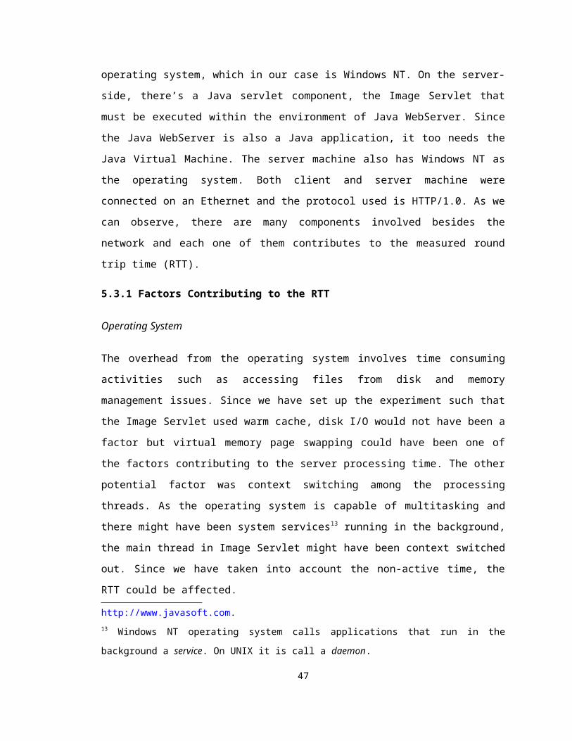
B.3 Pre-compressed algorithm data



1 781 781 741 762 761 751 751 762 770 761 762 13

2 511 511 521 521 510 530 521 521 520 510 518 7

3 461 461 461 461 450 440 812 461 450 460 492 113

4 430 440 430 430 431 431 430 440 431 431 432 4

5 431 441 431 440 431 441 441 430 441 441 437 5

6 441 431 441 441 440 440 431 441 440 440 439 4

7 340 340 340 341 351 351 340 350 341 341 344 5

8 440 441 441 440 431 441 451 440 441 441 441 5

9 351 351 351 351 340 350 351 351 350 360 351 5

10 491 491 490 501 491 491 480 491 491 481 490 6

11 350 340 340 350 341 341 341 340 341 351 344 5

12 351 351 341 351 340 340 351 351 350 340 347 5

13 450 450 450 451 451 461 440 450 451 451 451 5

14 350 340 351 360 341 341 361 360 341 351 350 9

15 351 411 371 351 340 340 340 341 340 350 354 22

16 450 501 470 451 451 441 340 460 441 461 447 41

6979 7081 6970 7002 6900 6930 7181 6989 6939 6970 6994 82

Note: The total time is the time taken to fetch all 16 images. Further operations on the images do

not add to the total time.

48

chapter 1 introduction - computing science - simon …stella/papers/simontangmsc.doc · web viewdr....

Documents